Embed Size (px)
Citation preview
NXTway-GS Model-Based Design - Control of self-balancing two-wheeled robot
built with LEGO Mindstorms NXT -

Author (First Edition) Yorihisa Yamamoto
Application Engineer
Advanced Support Group 1 Engineering Department
Applied Systems First Division
CYBERNET SYSTEMS CO., LTD.
Revision History
Revision Date Description Author / Editor
1.0 29 Feb 2008 First edition Yorihisa Yamamoto
1.1 3 Mar 2008 Added fixed-point controller model Yorihisa Yamamoto
Updated software [email protected]
1.2 7 Nov 2008
Modified motion equations
Modified annotations in controller models
Yorihisa Yamamoto
Updated software
1.3 28 Nov 2008
Modified generalized forces
Modified motion equations and state
equations
Added simulation movie
Yorihisa Yamamoto
1.4 1 May 2009 Modified text Yorihisa Yamamoto
The contents and URL described in this document can be changed with no previous notice.

Introduction
NXTway-GS is a self-balancing two-wheeled robot built with LEGO Mindstorms NXT. This document
presents Model-Based Design about balance and drive control of NXTway-GS by using MATALB / Simulink.
The main contents are the following.
Mathematical Model
Controller Design
Model Illustration
Simulation & Experimental Results
Preparation
To build NXTway-GS, read NXTway-GS Building Instructions.
You need to download Embedded Coder Robot NXT from the following URL because it is used as
Model-Based Design Environment in this document.
http://www.mathworks.com/matlabcentral/fileexchange/13399
Read Embedded Coder Robot NXT Instruction Manual (Embedded Coder Robot NXT Instruction
En.pdf) and test sample models / programs preliminarily. The software versions used in this document are as
follows.
Software Version
Embedded Coder Robot NXT 3.14
nxtOSEK (previous name is LEJOS OSEK) 2.03
Cygwin 1.5.24
GNU ARM 4.0.2
- i -
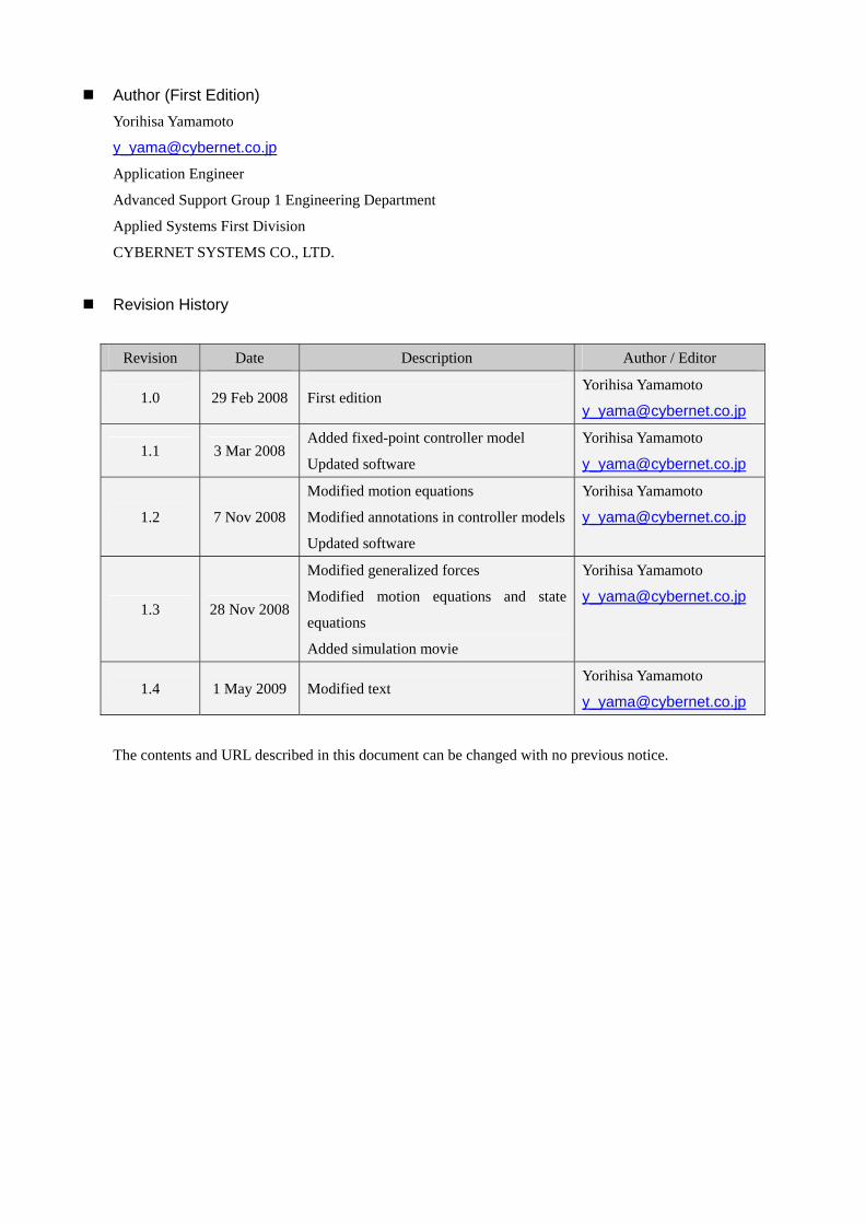
Required Products
Product Version Release
MATLAB® 7.5.0 R2007b
Control System Toolbox 8.0.1 R2007b
Simulink® 7.0 R2007b
Real-Time Workshop® 7.0 R2007b
Real-Time Workshop® Embedded Coder 5.0 R2007b
Fixed-Point Toolbox (N1) 2.1 R2007b
Simulink® Fixed Point (N1) 5.5 R2007b
Virtual Reality Toolbox (N2) 4.6 R2007b
You can simulate NXTway-GS models and generate codes from it without the products (N1) and (N2).
(N1) : It is required to run fixed-point arithmetic controller model (nxtway_gs_controller_fixpt.mdl).
(N2) : It is required to run 3D visualization (nxtway_gs_vr.mdl).
File List
File Description
iswall.m M-function for detecting wall in map
mywritevrtrack.m M-function for generating map file (track.wrl)
nxtway_gs.mdl NXTway-GS model (It does not require Virtual Reality Toolbox)
nxtway_gs_controller.mdl NXTway-GS controller model (single precision floating-point)
nxtway_gs_controller_fixpt.mdl NXTway-GS controller model (fixed-point)
nxtway_gs_plant.mdl NXTway-GS plant model
nxtway_gs_vr.mdl NXTway-GS model (It requires Virtual Reality Toolbox)
param_controller.m M-script for controller parameters
param_controller_fixpt.m M-script for fixed-point settings (Simulink.NumericType)
param_nxtway_gs.m M-script for NXTway-GS parameters (It calls param_***.m)
param_plant.m M-script for plant parameters
param_sim.m M-script for simulation parameters
track.bmp map image file
track.wrl map VRML file
vrnxtwaytrack.wrl map & NXTway-GS VRML file
- ii -
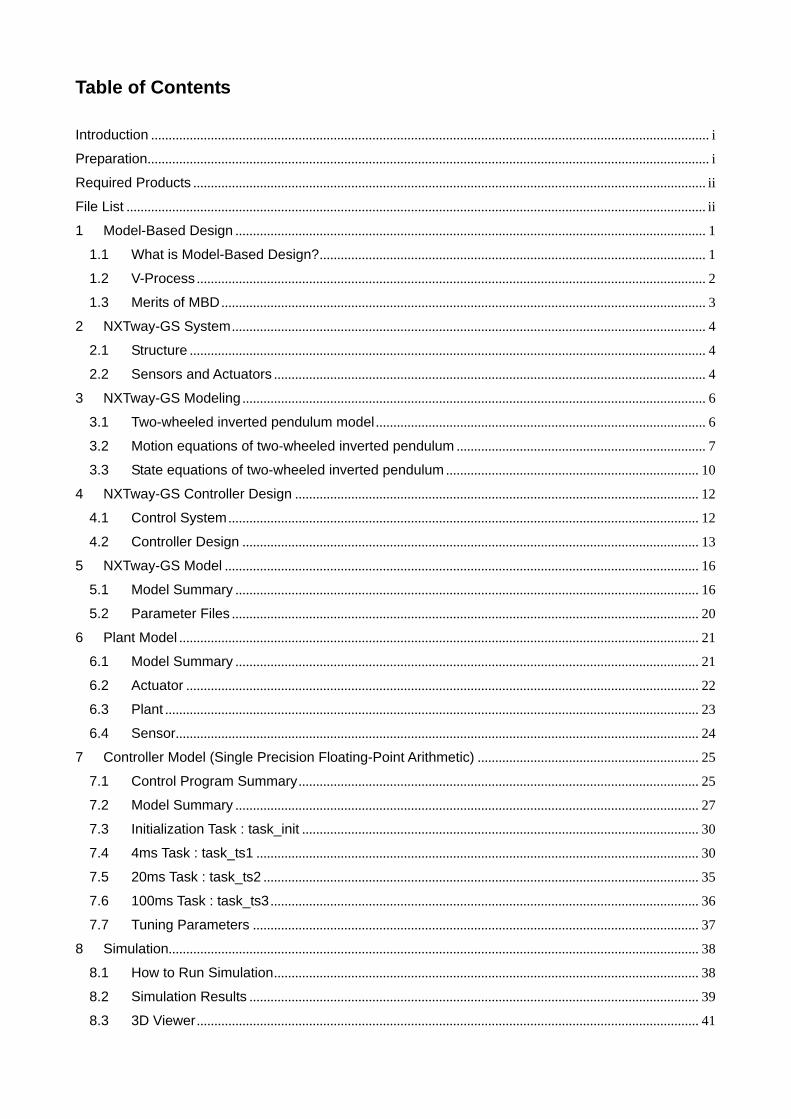
Table of Contents
Introduction ............................................................................................................................................................... i Preparation................................................................................................................................................................ i Required Products .................................................................................................................................................. ii File List ..................................................................................................................................................................... ii 1 Model-Based Design ...................................................................................................................................... 1
1.1 What is Model-Based Design?.............................................................................................................. 1 1.2 V-Process ................................................................................................................................................. 2 1.3 Merits of MBD .......................................................................................................................................... 3
2 NXTway-GS System ....................................................................................................................................... 4 2.1 Structure ................................................................................................................................................... 4 2.2 Sensors and Actuators ........................................................................................................................... 4
3 NXTway-GS Modeling .................................................................................................................................... 6 3.1 Two-wheeled inverted pendulum model .............................................................................................. 6 3.2 Motion equations of two-wheeled inverted pendulum ....................................................................... 7 3.3 State equations of two-wheeled inverted pendulum ........................................................................ 10
4 NXTway-GS Controller Design ................................................................................................................... 12 4.1 Control System ...................................................................................................................................... 12 4.2 Controller Design .................................................................................................................................. 13
5 NXTway-GS Model ....................................................................................................................................... 16 5.1 Model Summary .................................................................................................................................... 16 5.2 Parameter Files ..................................................................................................................................... 20
6 Plant Model .................................................................................................................................................... 21 6.1 Model Summary .................................................................................................................................... 21 6.2 Actuator .................................................................................................................................................. 22 6.3 Plant ........................................................................................................................................................ 23 6.4 Sensor..................................................................................................................................................... 24
7 Controller Model (Single Precision Floating-Point Arithmetic) ............................................................... 25 7.1 Control Program Summary .................................................................................................................. 25 7.2 Model Summary .................................................................................................................................... 27 7.3 Initialization Task : task_init ................................................................................................................. 30 7.4 4ms Task : task_ts1 .............................................................................................................................. 30 7.5 20ms Task : task_ts2 ............................................................................................................................ 35 7.6 100ms Task : task_ts3 .......................................................................................................................... 36 7.7 Tuning Parameters ............................................................................................................................... 37
8 Simulation....................................................................................................................................................... 38 8.1 How to Run Simulation......................................................................................................................... 38 8.2 Simulation Results ................................................................................................................................ 39 8.3 3D Viewer ............................................................................................................................................... 41
9 Code Generation and Implementation ....................................................................................................... 42 9.1 Target Hardware & Software ............................................................................................................... 42 9.2 How to Generate Code and Download .............................................................................................. 43 9.3 Experimental Results............................................................................................................................ 44
10 Controller Model (Fixed-Point Arithmetic) ............................................................................................. 46 10.1 What is Fixed-Point Number? ............................................................................................................. 46 10.2 Floating-Point to Fixed-Point Conversion.......................................................................................... 47 10.3 Simulation Results ................................................................................................................................ 50 10.4 Code Generation & Experimental Results......................................................................................... 51
11 Challenges for Readers ............................................................................................................................... 52 Appendix A Modern Control Theory ................................................................................................................ 53
A.1 Stability ..................................................................................................................................................... 53 A.2 State Feedback Control.......................................................................................................................... 53 A.3 Servo Control ........................................................................................................................................... 55
Appendix B Virtual Reality Space .................................................................................................................... 57 B.1 Coordinate System ................................................................................................................................. 57 B.2 Making Map File ...................................................................................................................................... 59 B.3 Distance Calculation and Wall Hit Detection....................................................................................... 60
Appendix C Generated Code ........................................................................................................................... 62 Reference............................................................................................................................................................... 66
- 1 -
1 Model-Based Design
This chapter outlines Model-Based Design briefly.
1.1 What is Model-Based Design?
Model-Based Design is a software development technique that uses simulation models. Generally, it is
abbreviated as MBD. For control systems, a designer models a plant and a controller or a part of them, and tests
the controller algorithm based on a PC simulation or real-time simulation. The real-time simulation enables us to
verify and validate the algorithm in real-time, by using code generated from the model. It is Rapid Prototyping
(RP) that a controller is replaced by a real-time simulator, and Hardware In the Loop Simulation (HILS) is a plant
version of Rapid Prototyping.
Furthermore, auto code generation products like RTW-EC enables us to generate C/C++ code for embedded
controllers (microprocessor, DSP, etc.) from the controller model. Figure 1-1 shows the MBD concept for control
systems based on MATLAB product family.
Simulink Stateflow Simulink Control Design Simulink Response OptimizationSimulink Parameter EstimationSimMechanics SimPowerSystems SimDriveline SimHydraulics Signal Processing Blockset Simulink Fixed Point
Control SystemDesign & Analysis SimulationEngineering
Problem
Mathematical Modeling
Code Generation
RP
HILS
EmbeddedSystem
Data
Data basedModeling
Prototyping Code (RTW)
Embedded Code (RTW-EC)
MATLAB
Data Acquisition Instrument Control OPC
Control System System Identification Fuzzy Logic Robust Control Model Predictive Control Neural Network Optimization Signal Processing Fixed-Point
Real-Time Workshop Real-Time Workshop Embedded Coder Stateflow Coder xPC Target
MATLAB Products (Toolbox) Simulink Products
Figure 1-1 MBD for control systems based on MATLAB product family
- 2 -
1.2 V-Process
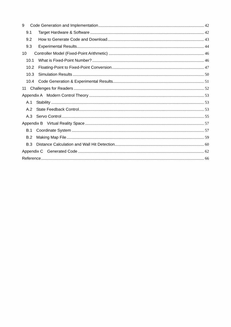
The V-process shown in Figure 1-2 describes the MBD development process for control systems. The V-process
consists of the Design, Coding, and Test stage. Each test stages correspond to the appropriate Design stages. A
developer makes plant / controller models in the left side of the V-process for early improvement of controller
algorithm, and reuses them in the right side for improvement of code verification and validation.
System Design
Module Design
Unit Design
Coding
Unit Test
Module Test
System Test
Product Test
Plant Modeling
Controller Algorithm Design
Code Generation for Embedded Systems
Verification Static Analysis Coding Rule Check
Early Improvement of Controller Algorithm
Improvement of CodeVerification & Validation
Product Design
Validation
Figure 1-2 V-process for control systems

- 3 -
1.3 Merits of MBD
MBD has the following merits.
Detection about specification errors in early stages of development
Hardware prototype reduction and fail-safe verification with real-time simulation
Efficient test by model verification
Effective communication by model usage
Coding time and error reduction by auto code generation
- 4 -
2 NXTway-GS System
This chapter describes the structure and sensors / actuators of NXTway-GS.
2.1 Structure
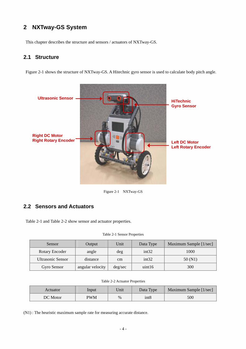
Figure 2-1 shows the structure of NXTway-GS. A Hitechnic gyro sensor is used to calculate body pitch angle.
HiTechnic Gyro Sensor
Ultrasonic Sensor
Left DC Motor Left Rotary Encoder
Right DC Motor Right Rotary Encoder
2.2 Sensors and Actuators
Table 2-1 and Table 2-2 show sensor and actuator properties.
(N1) : The heuristic maximum sample rate for measuring accurate distance.
Sensor Output Unit Data Type Maximum Sample [1/sec]
Rotary Encoder angle deg int32 1000
Ultrasonic Sensor distance cm int32 50 (N1)
Gyro Sensor angular velocity deg/sec uint16 300
Figure 2-1 NXTway-GS
Table 2-1 Sensor Properties
Table 2-2 Actuator Properties
Actuator Input Unit Data Type Maximum Sample [1/sec]
DC Motor PWM % int8 500

- 5 -
The reference [1] illustrates many properties about DC motor. Generally speaking, sensors and actuators are
different individually. Especially, you should note that gyro offset and gyro drift have big impact on balance
control. Gyro offset is an output when a gyro sensor does not rotate, and gyro drift is time variation of gyro
offset.
- 6 -
3 NXTway-GS Modeling
This chapter describes mathematical model and motion equations of NXTway-GS.
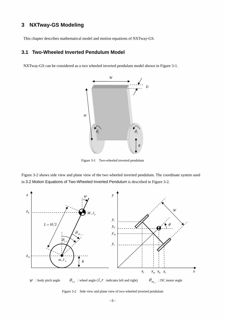
3.1 Two-Wheeled Inverted Pendulum Model
NXTway-GS can be considered as a two wheeled inverted pendulum model shown in Figure 3-1.
W
D
H
Figure 3-2 shows side view and plane view of the two wheeled inverted pendulum. The coordinate system used
in 3.2 Motion Equations of Two-Wheeled Inverted Pendulum is described in Figure 3-2.
ψ : body pitch angle rl ,θ : wheel angle ( indicates left and right) rl,rlm ,
θ : DC motor angle
lθrθ
R
Figure 3-1 Two-wheeled inverted pendulum
Figure 3-2 Side view and plane view of two-wheeled inverted pendulum
rl ,θ
yz
ry
mybyly
ψ
lx mx bx rx x
rlm ,θ
Wbz
mz
2HL =
ψJM ,
wJm,
φ
R
- 7 -
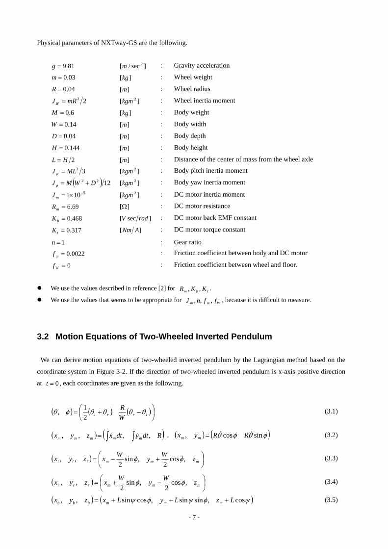
Physical parameters of NXTway-GS are the following.
: Gravity acceleration 81.9=g ]sec/[ 2m
: Wheel weight 03.0=m ][kg
: Wheel radius 04.0=R ][m
22mRJW = : Wheel inertia moment ][ 2kgm
: Body weight 6.0=M ][kg
: Body width 14.0=W ][m
: Body depth 04.0=D ][m
: Body height 144.0=H ][m
2HL = : Distance of the center of mass from the wheel axle ][m 32MLJ =ψ : Body pitch inertia moment ][ 2kgm
( ) 1222 DWMJ +=φ : Body yaw inertia moment ][ 2kgm
: DC motor inertia moment 5101 −×=mJ ][ 2kgm
: DC motor resistance 69.6=mR ][Ω
468.0=bK ]sec[ radV : DC motor back EMF constant
317.0=tK ][ ANm : DC motor torque constant
1=n : Gear ratio
0022.0=mf : Friction coefficient between body and DC motor
0=Wf : Friction coefficient between wheel and floor.
We use the values described in reference [2] for . tbm KKR ,,
We use the values that seems to be appropriate for , because it is difficult to measure. Wmm ffnJ ,,,
3.2 Motion Equations of Two-Wheeled Inverted Pendulum
We can derive motion equations of two-wheeled inverted pendulum by the Lagrangian method based on the
coordinate system in Figure 3-2. If the direction of two-wheeled inverted pendulum is x-axis positive direction
at , each coordinates are given as the following. 0=t
( ) ( ) ( ⎟⎠⎞
⎜⎝⎛ −+= lrrl W
R θθθθφθ21, ) (3.1)
( ) ( )Rdtydtxzyx mmmmm ,,,, ∫∫= && , ( ) ( )φθφθ sincos, &&&& RRyx mm = (3.2)
( ) ⎟⎠⎞
⎜⎝⎛ +−= mmmlll zWyWxzyx ,cos
2,sin
2,, φφ (3.3)
( ) ⎟⎠⎞
⎜⎝⎛ −+= mmmrrr zWyWxzyx ,cos
2,sin
2,, φφ (3.4)
( ) ( )ψφψφψ cos,sinsin,cossin,, LzLyLxzyx mmmbbb +++= (3.5)
- 8 -
The translational kinetic energy , the rotational kinetic energy , the potential energy are 1T 2T U
( ) ( ) ( )2222222221 2
121
21
bbbrrrlll zyxMzyxmzyxmT &&&&&&&&& ++++++++= (3.6)
222222222 )(
21)(
21
21
21
21
21 ψθψθφψθθ φψ &&&&&&&& −+−++++= rmlmrwlw JnJnJJJJT (3.7)
brl MgzmgzmgzU ++= (3.8)
The fifth and sixth term in are rotation kinetic energy of an armature in left and right DC motor. The
Lagrangian 2T
L has the following expression.
UTTL −+= 21 (3.9)
We use the following variables as the generalized coordinates.
θ : Average angle of left and right wheel
ψ : Body pitch angle
φ : Body yaw angle
Lagrange equations are the following
θθθFLL
dtd
=∂∂
−⎟⎠⎞
⎜⎝⎛∂∂&
(3.10)
ψψψFLL
dtd
=∂∂
−⎟⎟⎠
⎞⎜⎜⎝
⎛∂∂&
(3.11)
φφφFLL
dtd
=∂∂
−⎟⎟⎠
⎞⎜⎜⎝
⎛∂∂&
(3.12)
We derive the following equations by evaluating Eqs. (3.10) - (3.12).
( )[ ] ( ) θψψψψθ FMLRJnMLRJnJRMm mmw =−−++++ sin2cos222 2222 &&&&& (3.13)
( ) ( ) ψψ ψψφψψθψ FMLMgLJnJMLJnMLR mm =−−+++− cossinsin22cos 22222 &&&&& (3.14)
( ) φφ ψψφψφψ FMLMLJnJR
WJmW mw =+⎥⎦
⎤⎢⎣
⎡++++ cossin2sin
221 2222
2
22 &&&& (3.15)
- 9 -
In consideration of DC motor torque and viscous friction, the generalized forces are given as the following
( ) ( ⎟⎠⎞
⎜⎝⎛ −+= lrrl FF
RWFFFFFF2
,,,, ψφψθ ) (3.16)
lwlmltl ffinKF θθψ &&& −−+= )( (3.17)
rwrmrtr ffinKF θθψ &&& −−+= )( (3.18)
)()( rmlmrtlt ffinKinKF θψθψψ&&&& −−−−−−= (3.19)
where is the DC motor current. rli ,
We cannot use the DC motor current directly in order to control it because it is based on PWM (voltage) control. Therefore, we evaluate the relation between current and voltage using DC motor equation. If
the friction inside the motor is negligible, the DC motor equation is generally as follows rli , rlv ,
(3.20) rlmrlbrlrlm iRKviL ,,,, )( −−+= θψ &&&
Here we consider that the motor inductance is negligible and is approximated as zero. Therefore the current is
m
rlbrlrl R
Kvi
)( ,,,
θψ && −+= (3.21)
From Eq.(3.21), the generalized force can be expressed using the motor voltage.
( ) ( ) ψβθβαθ && 22 ++−+= wrl fvvF (3.22)
( ) ψβθβαψ && 22 −++−= rl vvF (3.23)
( ) ( φβαφ&
wlr f )R
WvvR
WF +−−= 2
2
22 (3.24)
mm
bt
m
t fR
KnKRnK
+== βα , (3.25)
- 10 -
3.3 State Equations of Two-Wheeled Inverted Pendulum
We can derive state equations based on modern control theory by linearizing motion equations at a balance point of NXTway-GS. It means that we consider the limit 0→ψ ( ψψ →sin , 1cos →ψ ) and neglect the
second order term like . The motion equations (3.13) – (3.15) are approximated as the following 2ψ&
( )[ ] ( ) θψθ FJnMLRJnJRMm mmw =−++++ &&&& 222 2222 (3.26)
( ) ( ) ψψ ψψθ FMgLJnJMLJnMLR mm =−+++− &&&& 222 22 (3.27)
( ) φφ φ FJnJR
WJmW mw =⎥⎦
⎤⎢⎣
⎡+++ &&2
2
22
221 (3.28)
Eq. (3.26) and Eq. (3.27) has θ and ψ , Eq. (3.28) has φ only. These equations can be expressed in the form
⎥⎦
⎤⎢⎣
⎡=⎥
⎦
⎤⎢⎣
⎡+⎥
⎦
⎤⎢⎣
⎡+⎥
⎦
⎤⎢⎣
⎡
r
l
vv
HGFEψθ
ψθ
ψθ
&
&
&&
&& (3.29)
( )
⎥⎦
⎤⎢⎣
⎡−−
=
⎥⎦
⎤⎢⎣
⎡−
=
⎥⎦
⎤⎢⎣
⎡−
−+=
⎥⎥⎦
⎤
⎢⎢⎣
⎡
++−−+++
=
αααα
ββββ
ψ
H
MgLG
fF
JnJMLJnMLRJnMLRJnJRMm
E
w
mm
mmw
000
2
222222
222
222
)( lr vvKJI −=+ φφ &&& (3.30)
( )
( )
α
β
φ
RWK
fR
WJ
JnJR
WJmWI
w
mw
2
2
221
2
2
22
22
=
+=
+++=
- 11 -
Here we consider the following variables as state, and as input. indicates transpose of . 21 xx , u Tx x
[ ] [ ] [ ]TrlTT
vv ,,,,,,, === uxx 21 φφψθψθ &&& (3.31)
Consequently, we can derive state equations of two-wheeled inverted pendulum from Eq. (3.29) and Eq. (3.30).
uxx 11 11 BA +=& (3.32)
uxx 22 22 BA +=& (3.33)
⎥⎥⎥⎥
⎦
⎤
⎢⎢⎢⎢
⎣
⎡
=
⎥⎥⎥⎥
⎦
⎤
⎢⎢⎢⎢
⎣
⎡
=
)4()4()3()3(
0000
,
)4,4()3,4()2,4(0)4,3()3,3()2,3(0
10000100
11
111
111
1111
BBBB
B
AAAAAA
A (3.34)
⎥⎦
⎤⎢⎣
⎡−
=⎥⎦
⎤⎢⎣
⎡−
=IKIK
BIJ
A00
,0
1022
(3.35)
( )[ ]( )[ ][ ][ ]
[ ][ ]
21
1
1
1
1
1
1
1
)2,1()2,2()1,1()det(
)det()2,1()1,1()4()det()2,1()2,2()3(
)det()2,1()1,1(2)4,4()det()2,1()2,2(2)4,3(
)det()1,1()2,1(2)3,4()det()2,1()2,2(2)3,3(
)det()1,1()2,4()det()2,1()2,3(
EEEE
EEEBEEEB
EEEAEEEA
EEEfAEEEfA
EgMLEAEgMLEA
w
w
−=
+−=+=
+−=+=
++=++−=
=−=
αα
ββ
ββββ
- 12 -
4 NXTway-GS Controller Design
This chapter describes the controller design of NXTway-GS (two-wheeled inverted pendulum) based on
modern control theory.
4.1 Control System
The characteristics as control system are as follows.
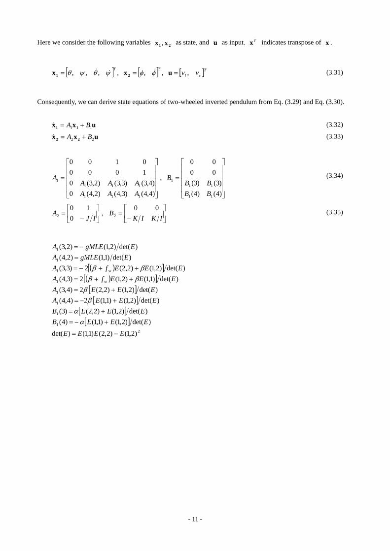
Inputs and Outputs
The input to an actuator is PWM duty of the left and right DC motor even though input in Eq. (3.31) is voltage. The outputs from sensors are the DC motor angle and the body pitch angular velocity
u
rlm ,θ ψ& .
DC Motor PWM
DC Motor Angle
Body Pitch Angular Velocity
Figure 4-1 Inputs and Outputs
It is easy to evaluate φθ , by using . There are two methods to evaluate
rlm ,θ ψ by using ψ& .
1. Derive ψ by integrating the angular speed numerically.
2. Estimate ψ by using an observer based on modern control theory.
We use method 1 in the following controller design.
Stability
It is easy to understand NXTway-GS balancing position is not stable. We have to move NXTway-GS in the
same direction of body pitch angle to keep balancing. Modern control theory gives many techniques to stabilize
an unstable system. (See Appendix A)
- 13 -
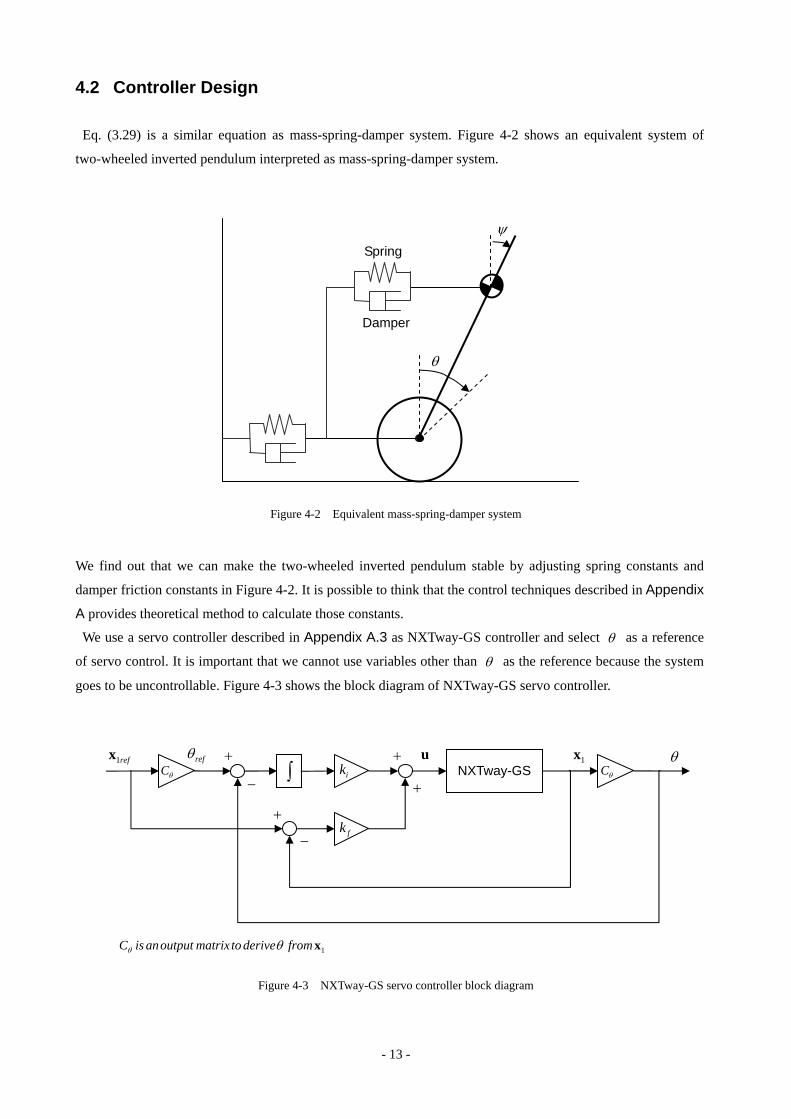
4.2 Controller Design
Eq. (3.29) is a similar equation as mass-spring-damper system. Figure 4-2 shows an equivalent system of
two-wheeled inverted pendulum interpreted as mass-spring-damper system.
θ
ψSpring
Damper
Figure 4-2 Equivalent mass-spring-damper system
We find out that we can make the two-wheeled inverted pendulum stable by adjusting spring constants and
damper friction constants in Figure 4-2. It is possible to think that the control techniques described in Appendix
A provides theoretical method to calculate those constants.
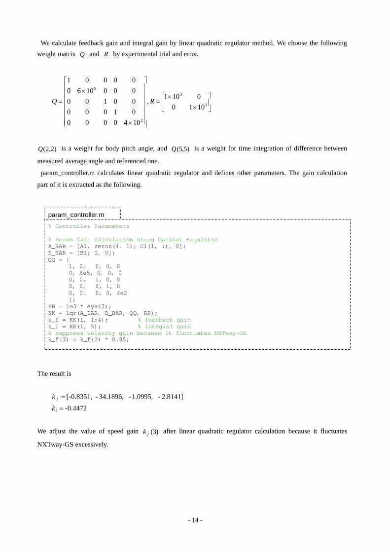
We use a servo controller described in Appendix A.3 as NXTway-GS controller and select θ as a reference
of servo control. It is important that we cannot use variables other than θ as the reference because the system
goes to be uncontrollable. Figure 4-3 shows the block diagram of NXTway-GS servo controller.
u 1x+
+
+ θ∫
−
+
−
θCref1x refθ
NXTway-GS
fk
ik θC
1xfromderivetomatrixoutputanisC θθ
Figure 4-3 NXTway-GS servo controller block diagram
- 14 -
We calculate feedback gain and integral gain by linear quadratic regulator method. We choose the following weight matrix and R by experimental trial and error. Q
⎥⎦
⎤⎢⎣
⎡
××
=
⎥⎥⎥⎥⎥⎥
⎦
⎤
⎢⎢⎢⎢⎢⎢
⎣
⎡
×
×= 3
3
2
5
10100101
,
10400000100000100000106000001
RQ
)2,2(Q is a weight for body pitch angle, and is a weight for time integration of difference between
measured average angle and referenced one.
)5,5(Q
param_controller.m calculates linear quadratic regulator and defines other parameters. The gain calculation
part of it is extracted as the following.
param_controller.m % Controller Parameters % Servo Gain Calculation using Optimal Regulator A_BAR = [A1, zeros(4, 1); C1(1, :), 0]; B_BAR = [B1; 0, 0]; QQ = [ 1, 0, 0, 0, 0 0, 6e5, 0, 0, 0 0, 0, 1, 0, 0 0, 0, 0, 1, 0 0, 0, 0, 0, 4e2 ]; RR = 1e3 * eye(3); KK = lqr(A_BAR, B_BAR, QQ, RR); k_f = KK(1, 1:4); % feedback gain k_i = KK(1, 5); % integral gain % suppress velocity gain because it fluctuates NXTway-GS k_f(3) = k_f(3) * 0.85;
The result is
-0.4472
]2.8141- 1.0995,- 34.1896,- -0.8351,[
=
=
i
f
k
k
We adjust the value of speed gain after linear quadratic regulator calculation because it fluctuates
NXTway-GS excessively.
)3(fk
- 15 -
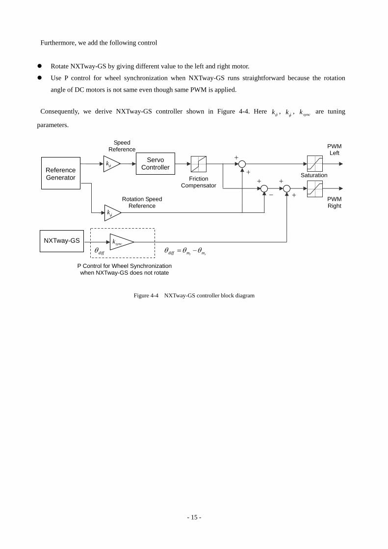
Furthermore, we add the following control
Rotate NXTway-GS by giving different value to the left and right motor.
Use P control for wheel synchronization when NXTway-GS runs straightforward because the rotation
angle of DC motors is not same even though same PWM is applied.
Consequently, we derive NXTway-GS controller shown in Figure 4-4. Here , , are tuning
parameters. θ&k φ&k synck
synck
θ&k
φ&k
NXTway-GS
Reference Generator
Servo Controller
diffθ
Speed Reference
Rotation SpeedReference
P Control for Wheel Synchronization when NXTway-GS does not rotate
Friction Compensator
+
++
−
+
+
Saturation
PWMLeft
PWMRight
rl mmdiff θθθ −=
Figure 4-4 NXTway-GS controller block diagram
- 16 -
5 NXTway-GS Model
This chapter describes summary of NXTway-GS model and parameter files.
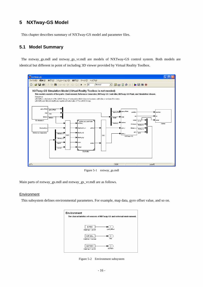
5.1 Model Summary
The nxtway_gs.mdl and nxtway_gs_vr.mdl are models of NXTway-GS control system. Both models are
identical but different in point of including 3D viewer provided by Virtual Reality Toolbox.
Figure 5-1 nxtway_gs.mdl
Main parts of nxtway_gs.mdl and nxtway_gs_vr.mdl are as follows.
Environment
This subsystem defines environmental parameters. For example, map data, gyro offset value, and so on.
Figure 5-2 Environment subsystem
- 17 -
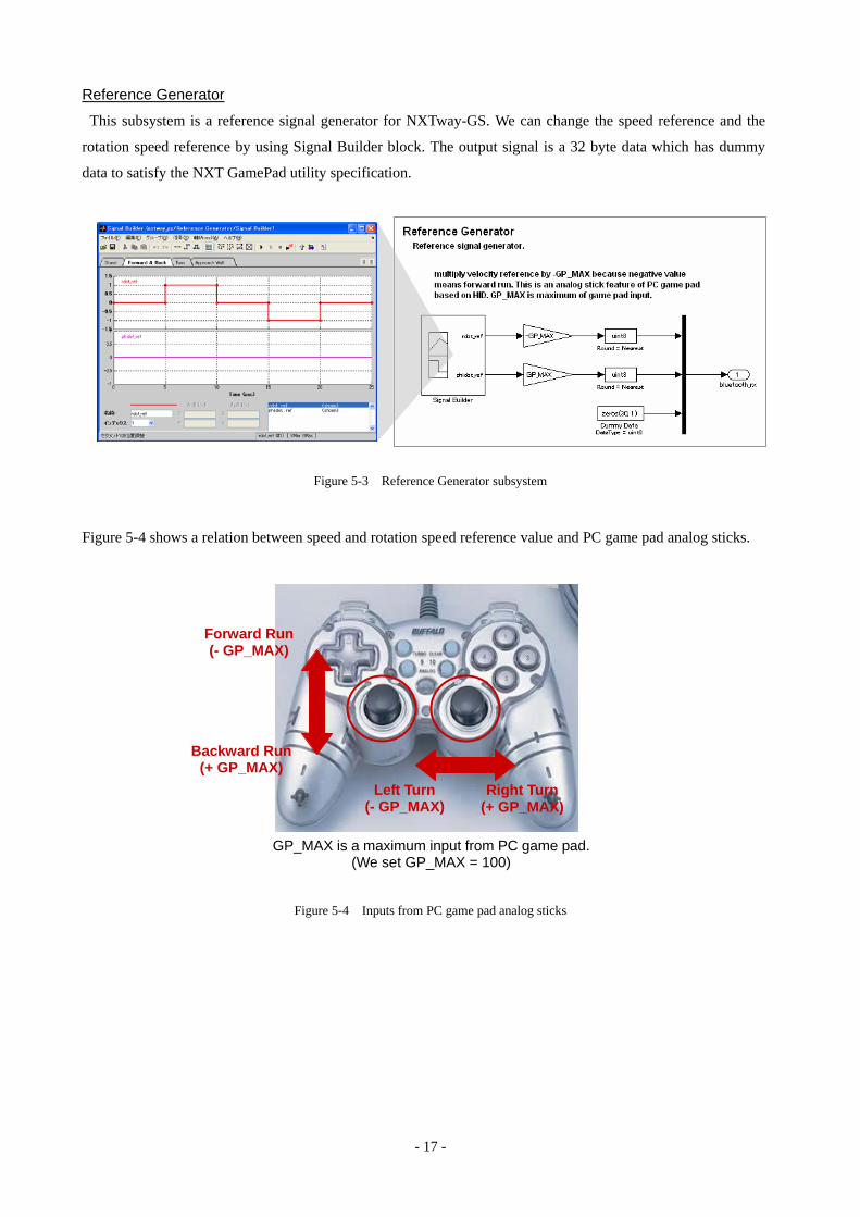
Reference Generator
This subsystem is a reference signal generator for NXTway-GS. We can change the speed reference and the
rotation speed reference by using Signal Builder block. The output signal is a 32 byte data which has dummy
data to satisfy the NXT GamePad utility specification.
Figure 5-3 Reference Generator subsystem
Figure 5-4 shows a relation between speed and rotation speed reference value and PC game pad analog sticks.
Forward Run (- GP_MAX)
Backward Run (+ GP_MAX)
Left Turn (- GP_MAX)
Right Turn(+ GP_MAX)
GP_MAX is a maximum input from PC game pad.
(We set GP_MAX = 100)
Figure 5-4 Inputs from PC game pad analog sticks
- 18 -
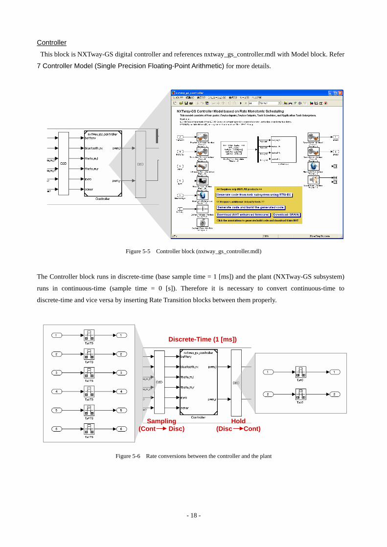
Controller
This block is NXTway-GS digital controller and references nxtway_gs_controller.mdl with Model block. Refer
7 Controller Model (Single Precision Floating-Point Arithmetic) for more details.
Figure 5-5 Controller block (nxtway_gs_controller.mdl)
The Controller block runs in discrete-time (base sample time = 1 [ms]) and the plant (NXTway-GS subsystem)
runs in continuous-time (sample time = 0 [s]). Therefore it is necessary to convert continuous-time to
discrete-time and vice versa by inserting Rate Transition blocks between them properly.
Discrete-Time (1 [ms])
Sampling (Cont Disc)
Hold (Disc Cont)
Figure 5-6 Rate conversions between the controller and the plant
- 19 -
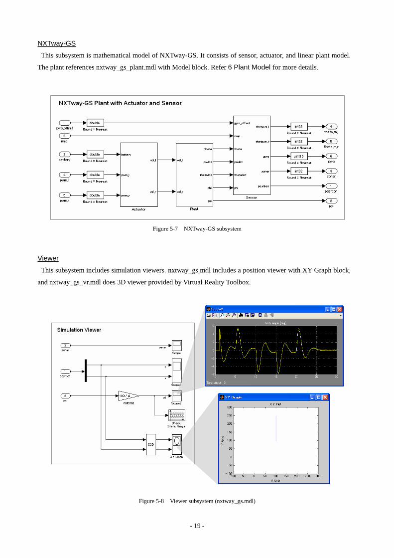
NXTway-GS
This subsystem is mathematical model of NXTway-GS. It consists of sensor, actuator, and linear plant model.
The plant references nxtway_gs_plant.mdl with Model block. Refer 6 Plant Model for more details.
Figure 5-7 NXTway-GS subsystem
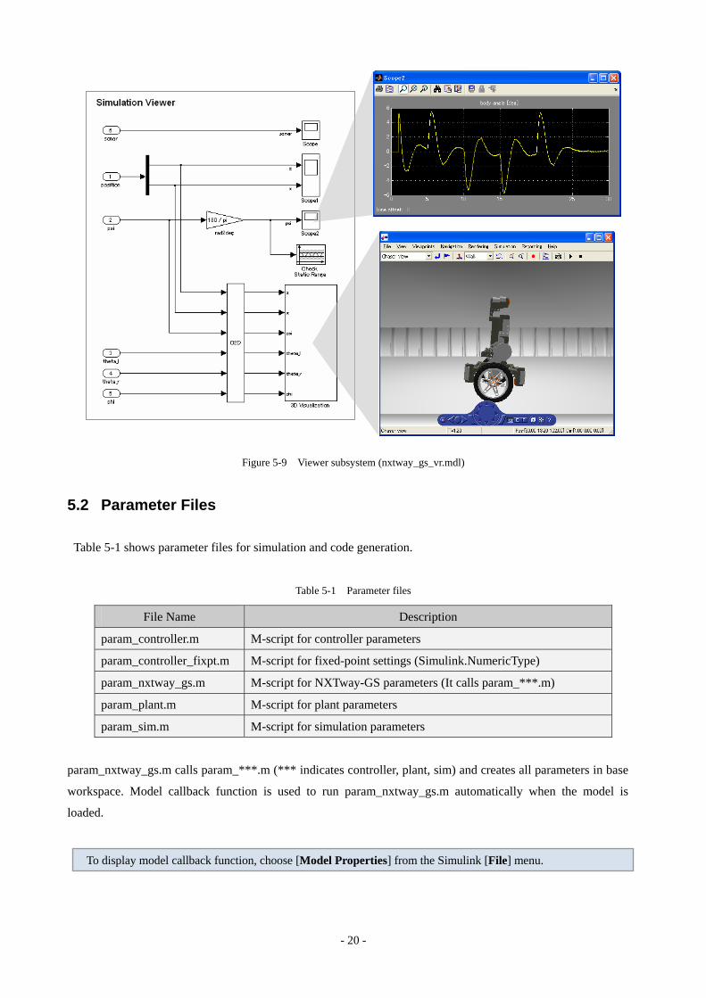
Viewer
This subsystem includes simulation viewers. nxtway_gs.mdl includes a position viewer with XY Graph block,
and nxtway_gs_vr.mdl does 3D viewer provided by Virtual Reality Toolbox.
Figure 5-8 Viewer subsystem (nxtway_gs.mdl)
- 20 -
5.2 Parameter Files
Table 5-1 shows parameter files for simulation and code generation.
Figure 5-9 Viewer subsystem (nxtway_gs_vr.mdl)
Table 5-1 Parameter files
File Name Description
param_controller.m M-script for controller parameters
param_controller_fixpt.m M-script for fixed-point settings (Simulink.NumericType)
param_nxtway_gs.m M-script for NXTway-GS parameters (It calls param_***.m)
param_plant.m M-script for plant parameters
param_sim.m M-script for simulation parameters
param_nxtway_gs.m calls param_***.m (*** indicates controller, plant, sim) and creates all parameters in base
workspace. Model callback function is used to run param_nxtway_gs.m automatically when the model is
loaded.
To display model callback function, choose [Model Properties] from the Simulink [File] menu.
- 21 -
6 Plant Model
This chapter describes NXTway-GS subsystem in nxtway_gs.mdl / nxtway_gs_vr.mdl.
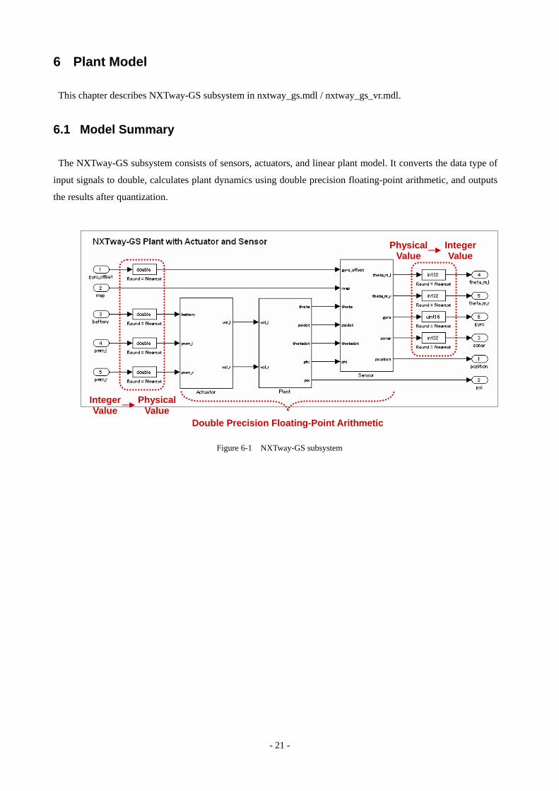
6.1 Model Summary
The NXTway-GS subsystem consists of sensors, actuators, and linear plant model. It converts the data type of
input signals to double, calculates plant dynamics using double precision floating-point arithmetic, and outputs
the results after quantization.
Integer Value
Double Precision Floating-Point Arithmetic
Physical Value
IntegerValue
Physical Value
Figure 6-1 NXTway-GS subsystem
- 22 -
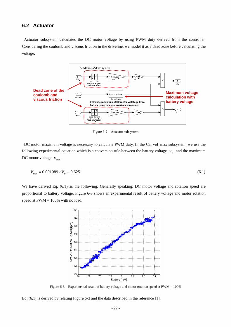
6.2 Actuator
Actuator subsystem calculates the DC motor voltage by using PWM duty derived from the controller.
Considering the coulomb and viscous friction in the driveline, we model it as a dead zone before calculating the
voltage.
Dead zone of the coulomb and viscous friction
Maximum voltage calculation with battery voltage
DC motor maximum voltage is necessary to calculate PWM duty. In the Cal vol_max subsystem, we use the following experimental equation which is a conversion rule between the battery voltage and the maximum
DC motor voltage . BV
maxV
(6.1) 625.0001089.0max −×= BVV
We have derived Eq. (6.1) as the following. Generally speaking, DC motor voltage and rotation speed are
proportional to battery voltage. Figure 6-3 shows an experimental result of battery voltage and motor rotation
speed at PWM = 100% with no load.
Figure 6-3 Experimental result of battery voltage and motor rotation speed at PWM = 100%
Figure 6-2 Actuator subsystem
Eq. (6.1) is derived by relating Figure 6-3 and the data described in the reference [1].
- 23 -
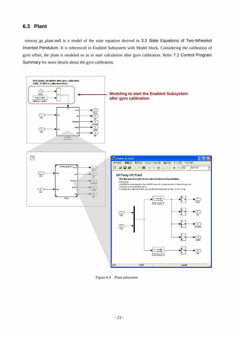
6.3 Plant
nxtway_gs_plant.mdl is a model of the state equation derived in 3.3 State Equations of Two-Wheeled
Inverted Pendulum. It is referenced in Enabled Subsystem with Model block. Considering the calibration of
gyro offset, the plant is modeled so as to start calculation after gyro calibration. Refer 7.1
Control Program
Summary for more details about the gyro calibration.
Modeling to start the Enabled Subsystem after gyro calibration
Figure 6-4 Plant subsystem
- 24 -
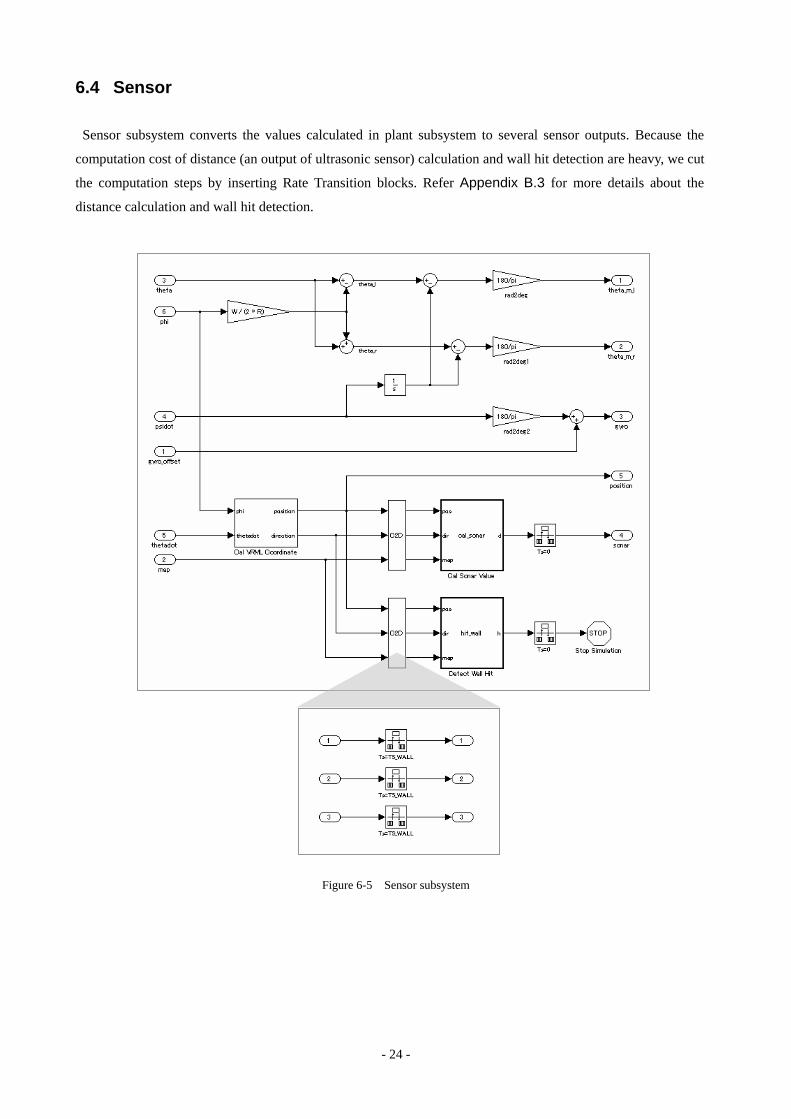
6.4 Sensor
Sensor subsystem converts the values calculated in plant subsystem to several sensor outputs. Because the
computation cost of distance (an output of ultrasonic sensor) calculation and wall hit detection are heavy, we cut
the computation steps by inserting Rate Transition blocks. Refer Appendix B.3 for more details about the
distance calculation and wall hit detection.
Figure 6-5 Sensor subsystem
- 25 -
7 Controller Model (Single Precision Floating-Point Arithmetic)
This chapter describes control program, task configuration, and model contents of nxtway_gs_controller.mdl.
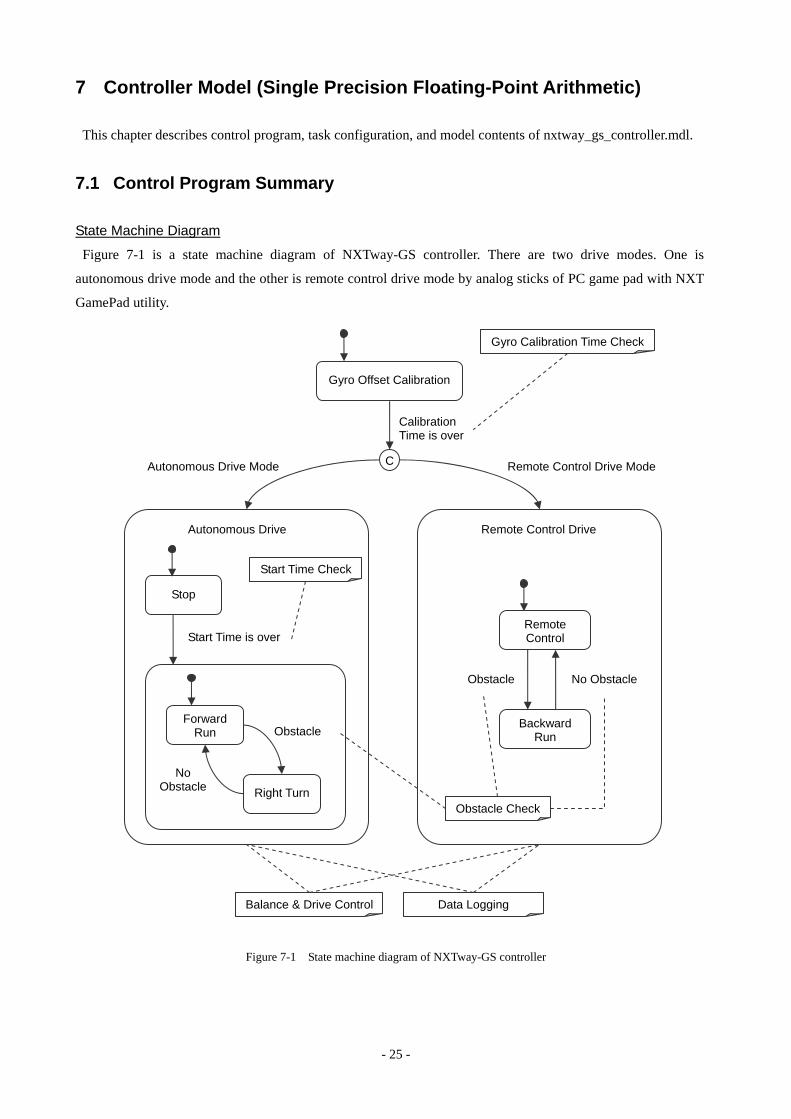
7.1 Control Program Summary
State Machine Diagram
Figure 7-1 is a state machine diagram of NXTway-GS controller. There are two drive modes. One is
autonomous drive mode and the other is remote control drive mode by analog sticks of PC game pad with NXT
GamePad utility.
Calibration Time is over
Gyro Calibration Time Check
Start Time Check
Obstacle Check
Balance & Drive Control Data Logging
Gyro Offset Calibration
Forward Run
Right Turn
Obstacle
Stop
Start Time is over
Autonomous Drive
Remote Control
Backward Run
Obstacle No Obstacle
Remote Control Drive
CAutonomous Drive Mode Remote Control Drive Mode
No Obstacle
Figure 7-1 State machine diagram of NXTway-GS controller
- 26 -
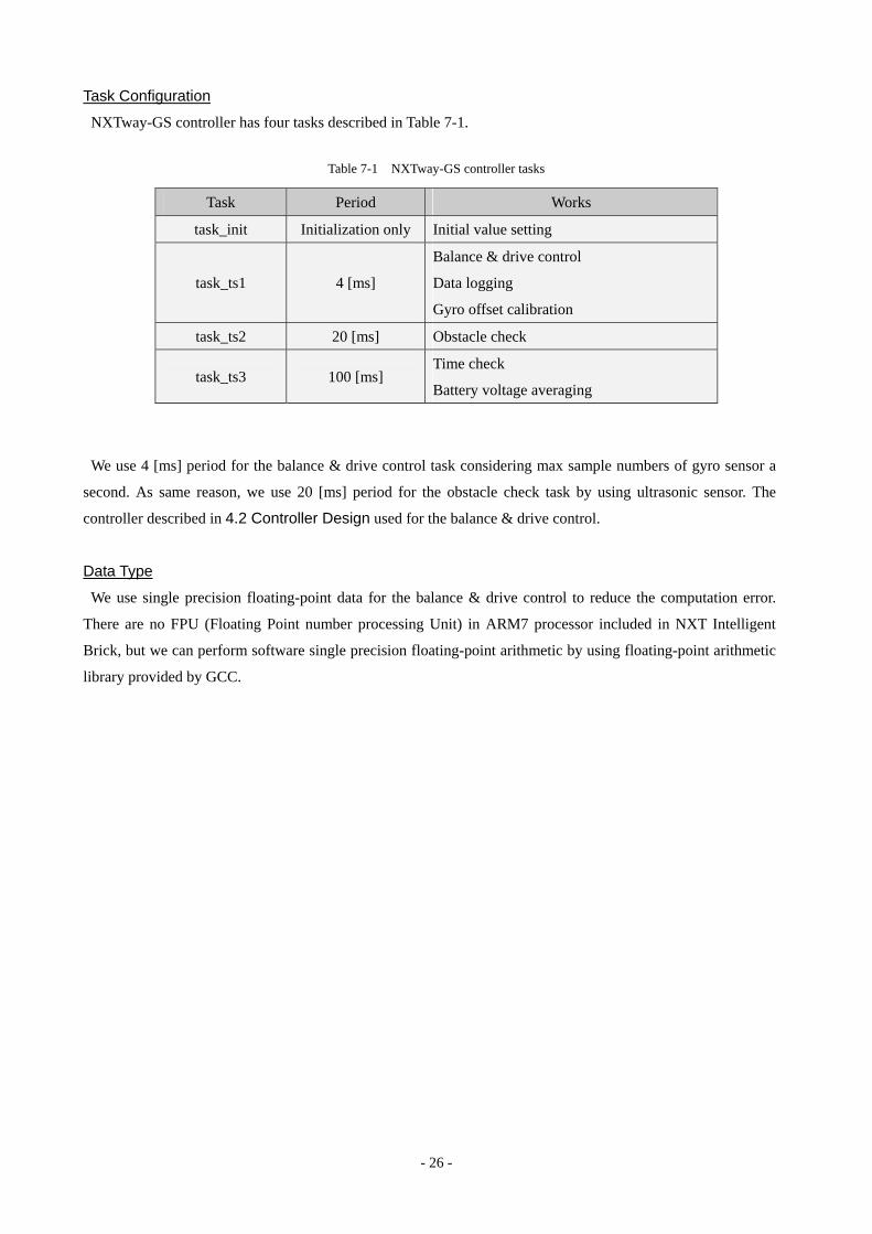
Task Configuration
NXTway-GS controller has four tasks described in Table 7-1.
Table 7-1 NXTway-GS controller tasks
Task Period Works
task_init Initialization only Initial value setting
task_ts1 4 [ms]
Balance & drive control
Data logging
Gyro offset calibration
task_ts2 20 [ms] Obstacle check
task_ts3 100 [ms]
Time check Battery voltage averaging
We use 4 [ms] period for the balance & drive control task considering max sample numbers of gyro sensor a
second. As same reason, we use 20 [ms] period for the obstacle check task by using ultrasonic sensor. The
controller described in 4.2 Controller Design used for the balance & drive control.
Data Type
We use single precision floating-point data for the balance & drive control to reduce the computation error.
There are no FPU (Floating Point number processing Unit) in ARM7 processor included in NXT Intelligent
Brick, but we can perform software single precision floating-point arithmetic by using floating-point arithmetic
library provided by GCC.
- 27 -
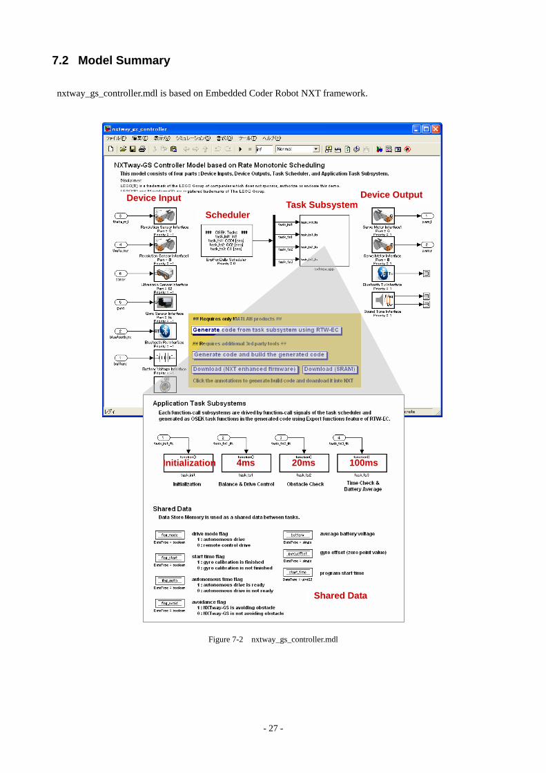
7.2 Model Summary
nxtway_gs_controller.mdl is based on Embedded Coder Robot NXT framework.
Device Input Device Output
SchedulerTask Subsystem
Initialization 4ms 20ms 100ms
Shared Data
Figure 7-2 nxtway_gs_controller.mdl
- 28 -
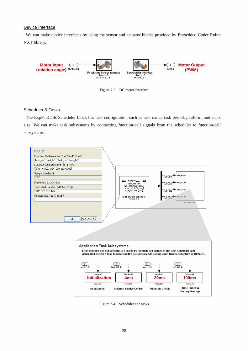
Device Interface
We can make device interfaces by using the sensor and actuator blocks provided by Embedded Coder Robot
NXT library.
Motor Input (rotation angle)
Motor Output (PWM)
Figure 7-3 DC motor interface
Scheduler & Tasks
The ExpFcnCalls Scheduler block has task configuration such as task name, task period, platform, and stack
size. We can make task subsystems by connecting function-call signals from the scheduler to function-call
subsystems.
Initialization 4ms 20ms 100ms
Figure 7-4 Scheduler and tasks
- 29 -
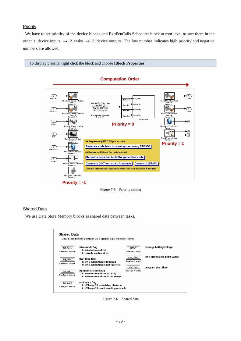
Priority
We have to set priority of the device blocks and ExpFcnCalls Scheduler block at root level to sort them in the
order 1. device inputs 2. tasks → 3. device outputs. The low number indicates high priority and negative
numbers are allowed.
→
To display priority, right click the block and choose [Block Properties].
Computation Order
Priority = -1
Priority = 0
Priority = 1
Figure 7-5 Priority setting
Shared Data
We use Data Store Memory blocks as shared data between tasks.
Figure 7-6 Shared data
- 30 -
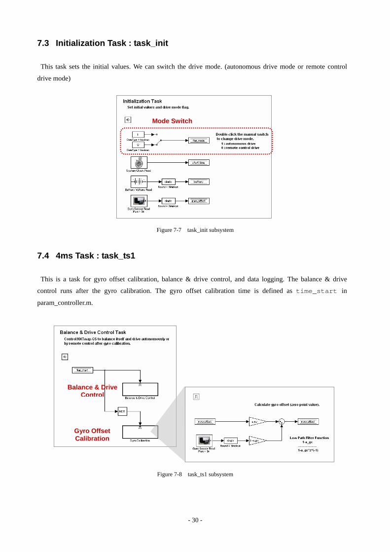
7.3 Initialization Task : task_init
This task sets the initial values. We can switch the drive mode. (autonomous drive mode or remote control
drive mode)
Mode Switch
Figure 7-7 task_init subsystem
7.4 4ms Task : task_ts1
This is a task for gyro offset calibration, balance & drive control, and data logging. The balance & drive
control runs after the gyro calibration. The gyro offset calibration time is defined as time_start in
param_controller.m.
Balance & Drive Control
Gyro Offset Calibration
Figure 7-8 task_ts1 subsystem
- 31 -
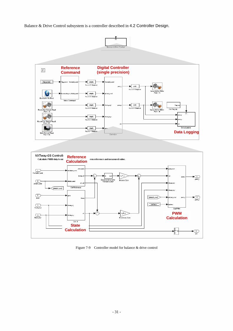
Balance & Drive Control subsystem is a controller described in 4.2 .Controller Design
Reference Command
Digital Controller (single precision)
Data Logging
Reference Calculation
State Calculation
PWM Calculation
Figure 7-9 Controller model for balance & drive control
- 32 -
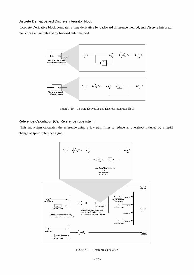
Discrete Derivative and Discrete Integrator block
Discrete Derivative block computes a time derivative by backward difference method, and Discrete Integrator
block does a time integral by forward euler method.
Figure 7-10 Discrete Derivative and Discrete Integrator block
Reference Calculation (Cal Reference subsystem)
This subsystem calculates the reference using a low path filter to reduce an overshoot induced by a rapid
change of speed reference signal.
Figure 7-11 Reference calculation
- 33 -
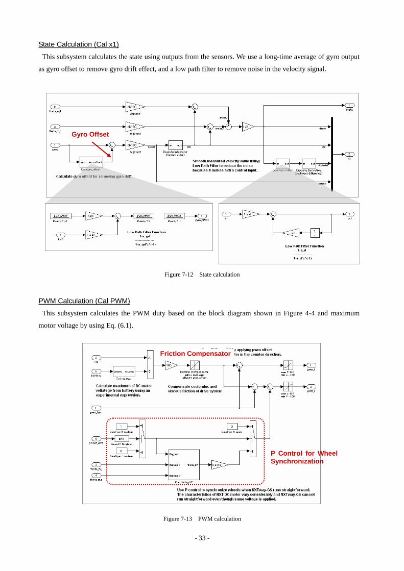
State Calculation (Cal x1)
This subsystem calculates the state using outputs from the sensors. We use a long-time average of gyro output
as gyro offset to remove gyro drift effect, and a low path filter to remove noise in the velocity signal.
Gyro Offset
Figure 7-12 State calculation
PWM Calculation (Cal PWM)
This subsystem calculates the PWM duty based on the block diagram shown in Figure 4-4 and maximum
motor voltage by using Eq. (6.1).
P Control for Wheel Synchronization
Friction Compensator
Figure 7-13 PWM calculation
- 34 -
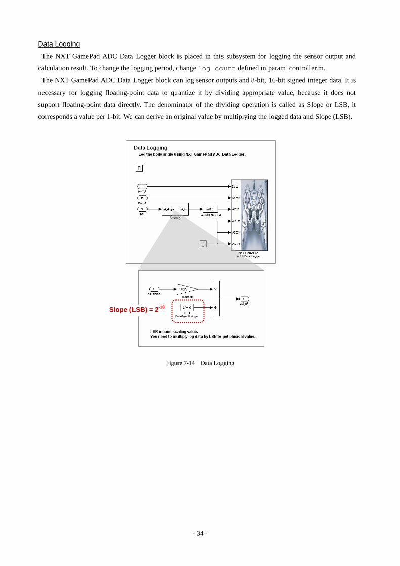
Data Logging
The NXT GamePad ADC Data Logger block is placed in this subsystem for logging the sensor output and
calculation result. To change the logging period, change log_count defined in param_controller.m.
The NXT GamePad ADC Data Logger block can log sensor outputs and 8-bit, 16-bit signed integer data. It is
necessary for logging floating-point data to quantize it by dividing appropriate value, because it does not
support floating-point data directly. The denominator of the dividing operation is called as Slope or LSB, it
corresponds a value per 1-bit. We can derive an original value by multiplying the logged data and Slope (LSB).
Slope (LSB) = 2-10
Figure 7-14 Data Logging
- 35 -
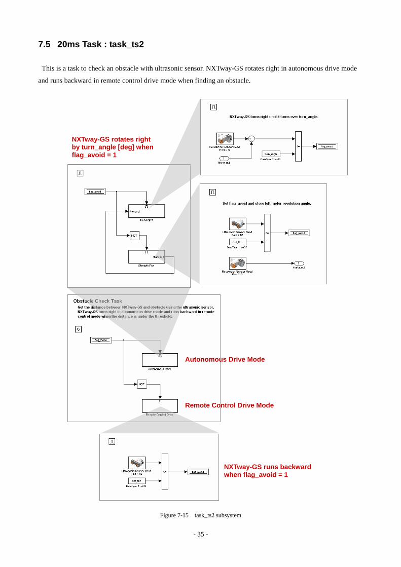
7.5 20ms Task : task_ts2
This is a task to check an obstacle with ultrasonic sensor. NXTway-GS rotates right in autonomous drive mode
and runs backward in remote control drive mode when finding an obstacle.
Autonomous Drive Mode
Remote Control Drive Mode
NXTway-GS rotates right by turn_angle [deg] when flag_avoid = 1
NXTway-GS runs backward when flag_avoid = 1
Figure 7-15 task_ts2 subsystem
- 36 -
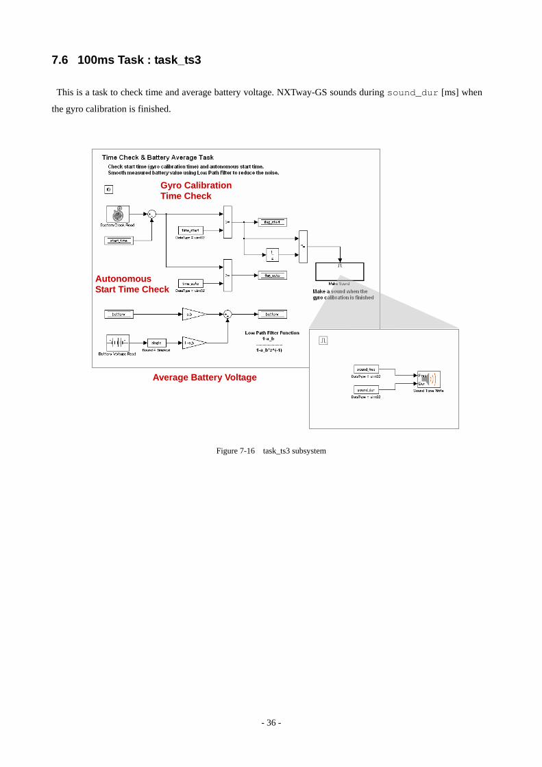
7.6 100ms Task : task_ts3
This is a task to check time and average battery voltage. NXTway-GS sounds during sound_dur [ms] when
the gyro calibration is finished.
Average Battery Voltage
Gyro Calibration Time Check
Autonomous Start Time Check
Figure 7-16 task_ts3 subsystem
- 37 -
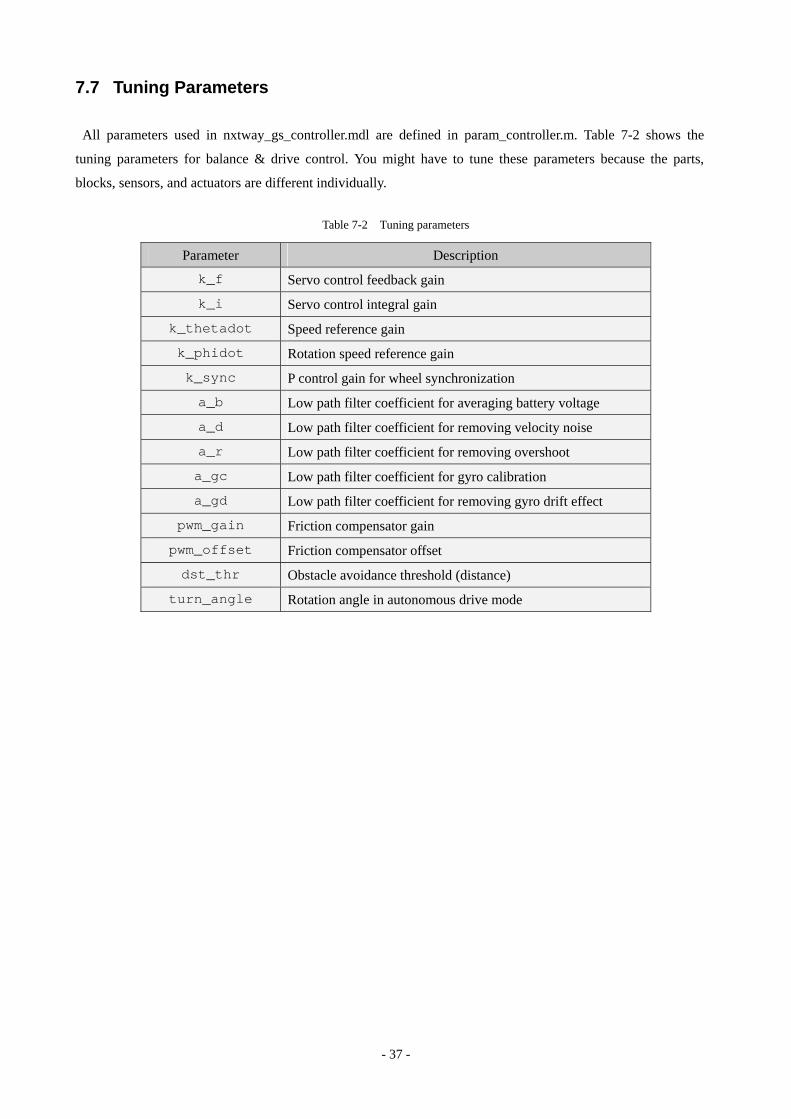
7.7 Tuning Parameters
All parameters used in nxtway_gs_controller.mdl are defined in param_controller.m. Table 7-2 shows the
tuning parameters for balance & drive control. You might have to tune these parameters because the parts,
blocks, sensors, and actuators are different individually.
Table 7-2 Tuning parameters
Parameter Description
k_f Servo control feedback gain
k_i Servo control integral gain
k_thetadot Speed reference gain
k_phidot Rotation speed reference gain
k_sync P control gain for wheel synchronization
a_b Low path filter coefficient for averaging battery voltage
a_d Low path filter coefficient for removing velocity noise
a_r Low path filter coefficient for removing overshoot
a_gc Low path filter coefficient for gyro calibration
a_gd Low path filter coefficient for removing gyro drift effect
pwm_gain Friction compensator gain
pwm_offset Friction compensator offset
dst_thr Obstacle avoidance threshold (distance)
turn_angle Rotation angle in autonomous drive mode
- 38 -
8 Simulation
This chapter describes simulation of NXTway-GS model, its result, and 3D viewer in nxtway_gs_vr.mdl.
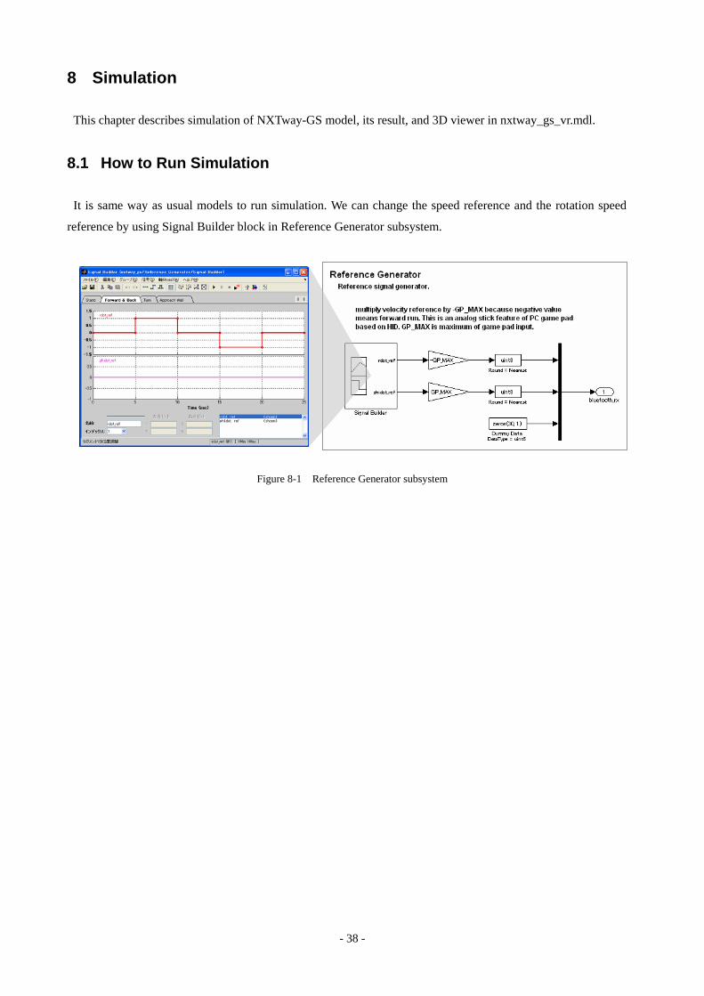
8.1 How to Run Simulation
It is same way as usual models to run simulation. We can change the speed reference and the rotation speed
reference by using Signal Builder block in Reference Generator subsystem.
Figure 8-1 Reference Generator subsystem
- 39 -
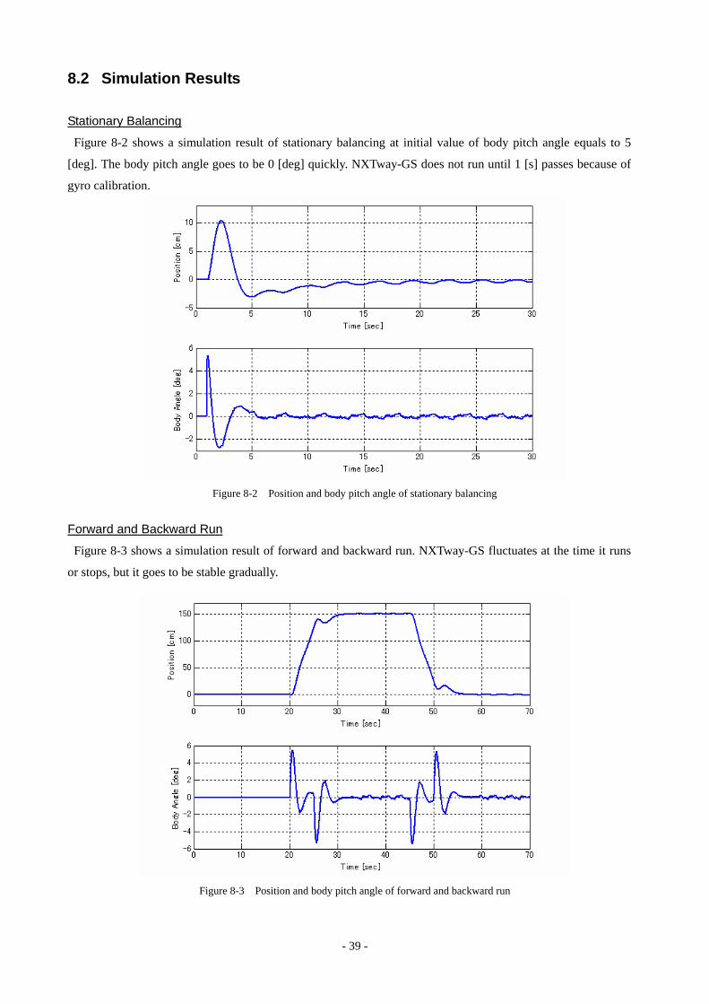
8.2 Simulation Results
Stationary Balancing
Figure 8-2 shows a simulation result of stationary balancing at initial value of body pitch angle equals to 5
[deg]. The body pitch angle goes to be 0 [deg] quickly. NXTway-GS does not run until 1 [s] passes because of
gyro calibration.
Figure 8-2 Position and body pitch angle of stationary balancing
Forward and Backward Run
Figure 8-3 shows a simulation result of forward and backward run. NXTway-GS fluctuates at the time it runs
or stops, but it goes to be stable gradually.
Figure 8-3 Position and body pitch angle of forward and backward run
- 40 -
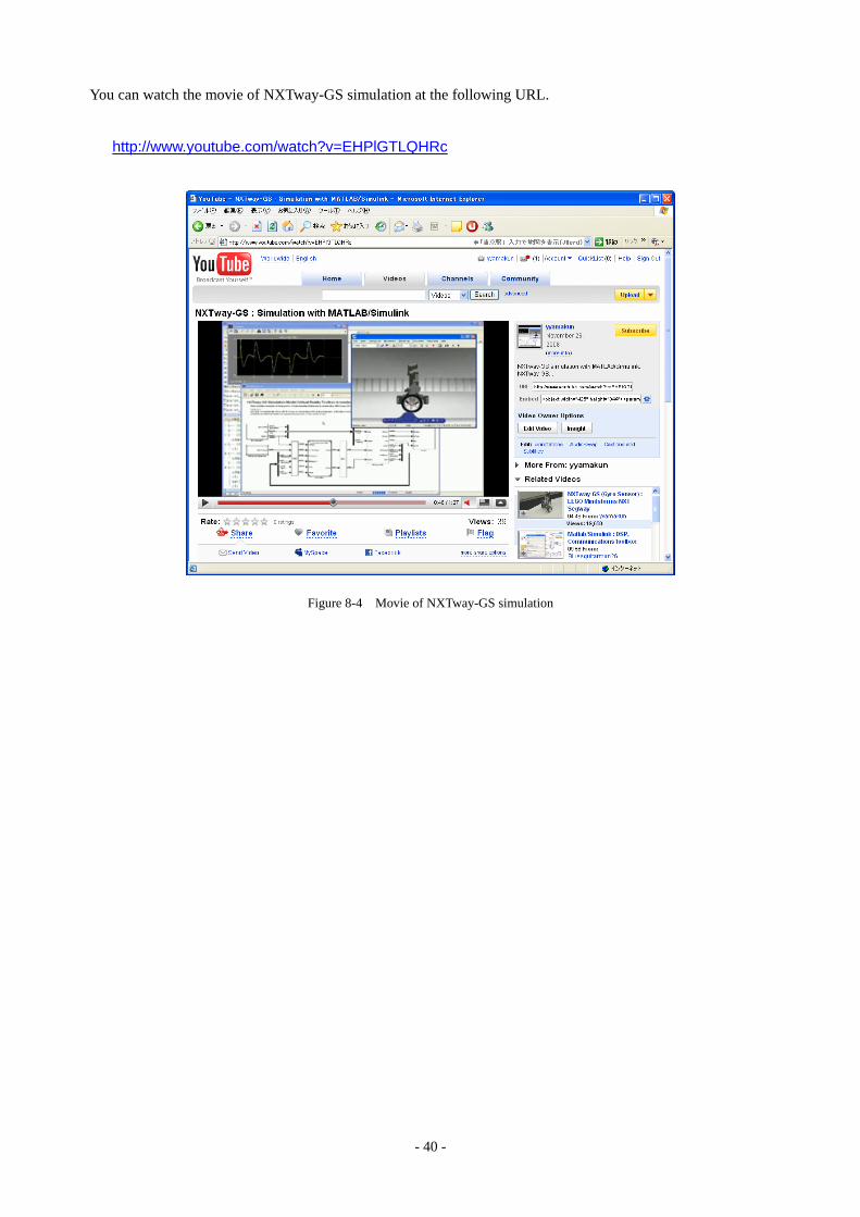
You can watch the movie of NXTway-GS simulation at the following URL.
http://www.youtube.com/watch?v=EHPlGTLQHRc
Figure 8-4 Movie of NXTway-GS simulation
- 41 -
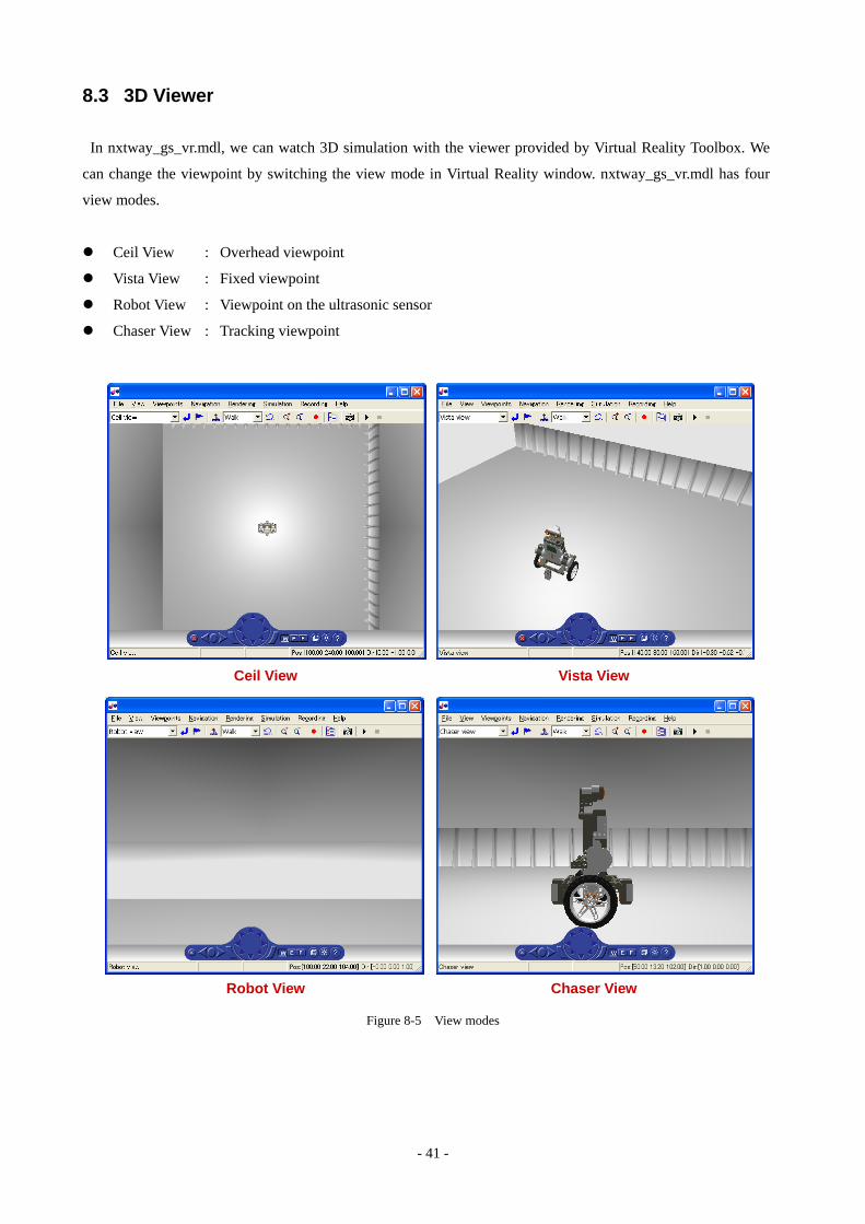
8.3 3D Viewer
In nxtway_gs_vr.mdl, we can watch 3D simulation with the viewer provided by Virtual Reality Toolbox. We
can change the viewpoint by switching the view mode in Virtual Reality window. nxtway_gs_vr.mdl has four
view modes.
Ceil View : Overhead viewpoint
Vista View : Fixed viewpoint
Robot View : Viewpoint on the ultrasonic sensor
Chaser View : Tracking viewpoint
Ceil View Vista View
Robot View Chaser View
Figure 8-5 View modes
- 42 -
9 Code Generation and Implementation
This chapter describes how to generate code from nxtway_gs_controller.mdl and download it into NXT
Intelligent Brick, and the experimental results are shown.
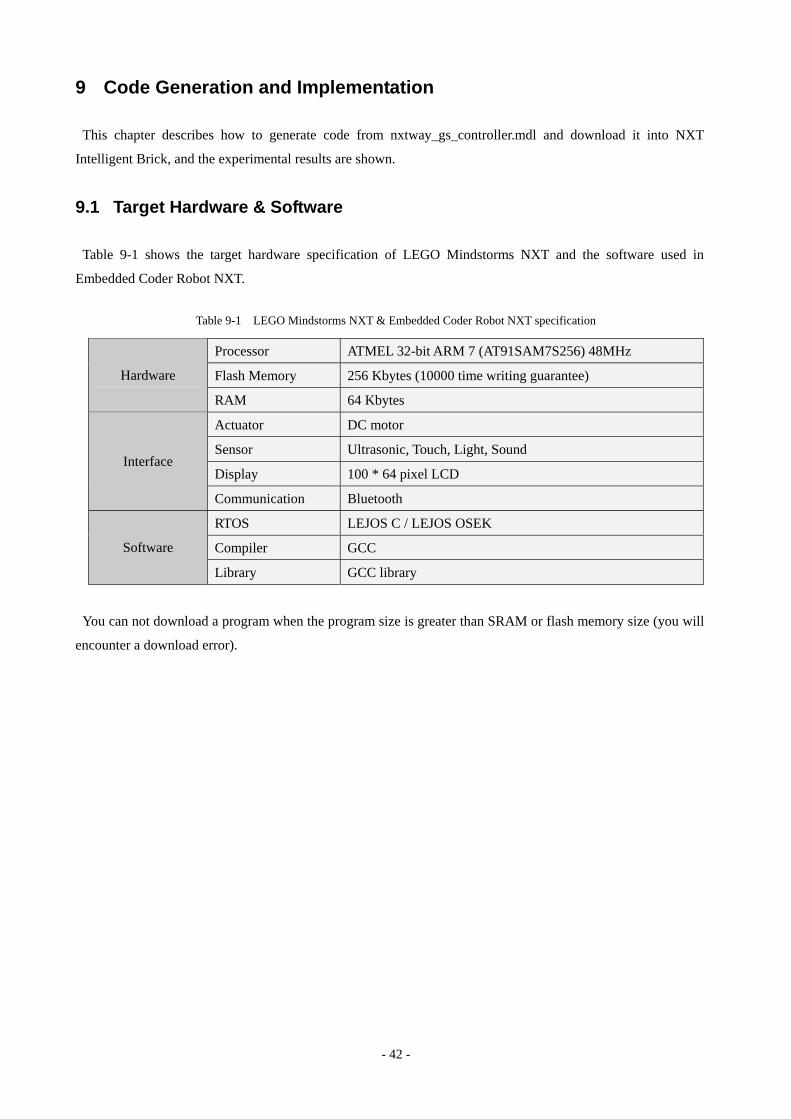
9.1 Target Hardware & Software
Table 9-1 shows the target hardware specification of LEGO Mindstorms NXT and the software used in
Embedded Coder Robot NXT.
Table 9-1 LEGO Mindstorms NXT & Embedded Coder Robot NXT specification
Processor ATMEL 32-bit ARM 7 (AT91SAM7S256) 48MHz
Flash Memory 256 Kbytes (10000 time writing guarantee) Hardware
RAM 64 Kbytes
Actuator DC motor
Sensor Ultrasonic, Touch, Light, Sound
Display 100 * 64 pixel LCD Interface
Communication Bluetooth
RTOS LEJOS C / LEJOS OSEK
Compiler GCC Software
Library GCC library
You can not download a program when the program size is greater than SRAM or flash memory size (you will
encounter a download error).
- 43 -
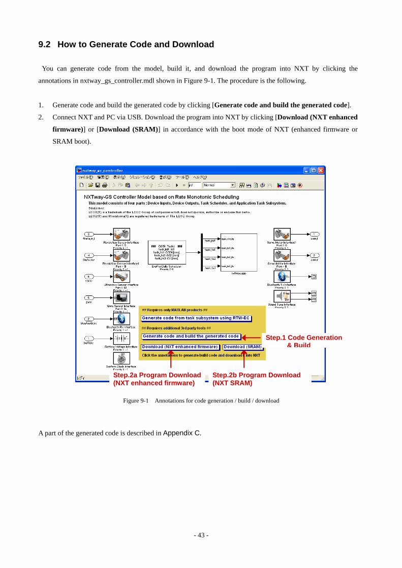
9.2 How to Generate Code and Download
You can generate code from the model, build it, and download the program into NXT by clicking the
annotations in nxtway_gs_controller.mdl shown in Figure 9-1. The procedure is the following.
1. Generate code and build the generated code by clicking [Generate code and build the generated code].
2. Connect NXT and PC via USB. Download the program into NXT by clicking [Download (NXT enhanced
firmware)] or [Download (SRAM)] in accordance with the boot mode of NXT (enhanced firmware or
SRAM boot).
Step.1 Code Generation & Build
Step.2a Program Download(NXT enhanced firmware)
Step.2b Program Download (NXT SRAM)
Figure 9-1 Annotations for code generation / build / download
A part of the generated code is described in Appendix C.
- 44 -
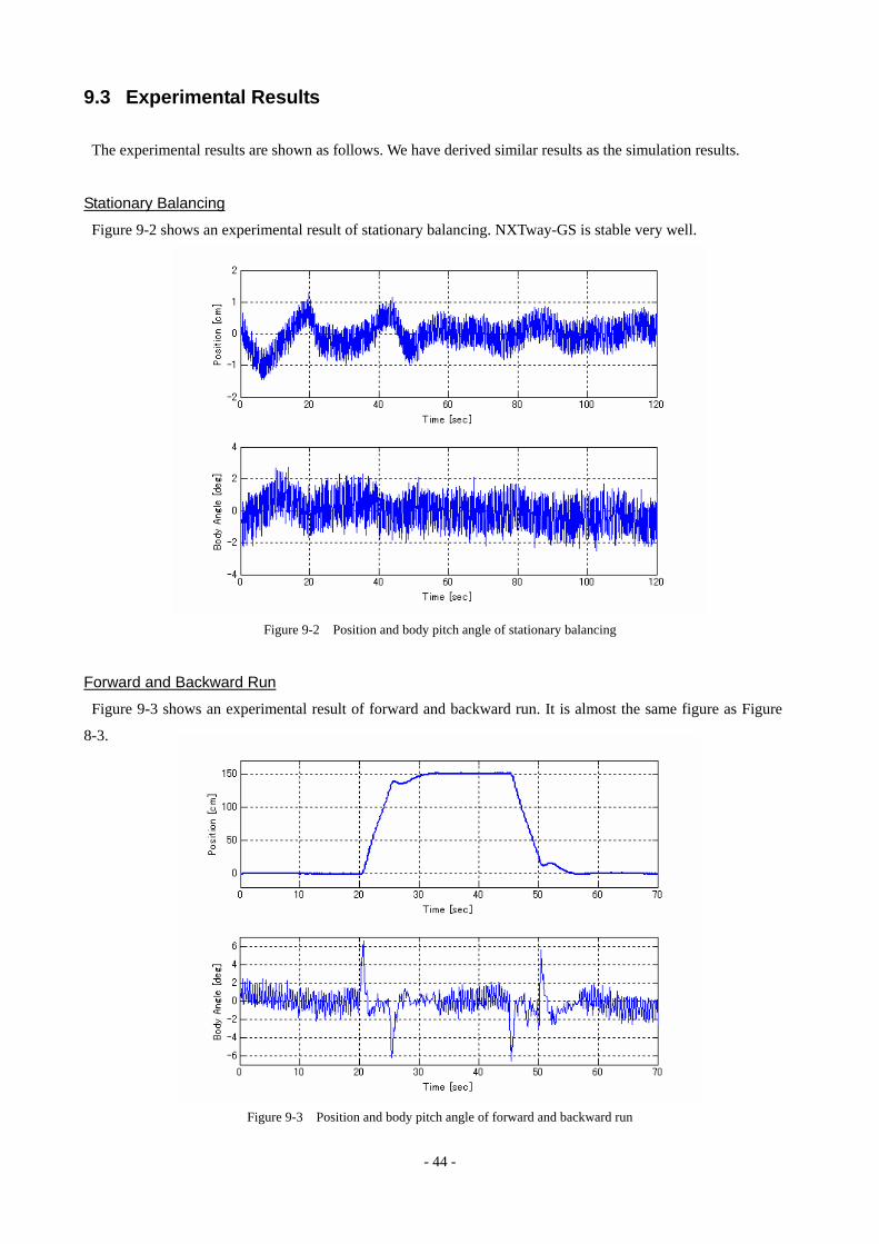
9.3 Experimental Results
The experimental results are shown as follows. We have derived similar results as the simulation results.
Stationary Balancing
Figure 9-2 shows an experimental result of stationary balancing. NXTway-GS is stable very well.
Figure 9-2 Position and body pitch angle of stationary balancing
Forward and Backward Run
Figure 9-3 shows an experimental result of forward and backward run. It is almost the same figure as Figure
8-3.
Figure 9-3 Position and body pitch angle of forward and backward run
- 45 -
You can watch the movie of NXTway-GS control experiment at the following URL.
http://www.youtube.com/watch?v=4ulBRQKCwd4
Figure 9-4 Movie of NXTway-GS control experiment
- 46 -
QR +=≅
10 Controller Model (Fixed-Point Arithmetic)
This chapter describes the fixed-point version of NXTway-GS controller model and considers a precision loss
and overflow impact on the controller performance.
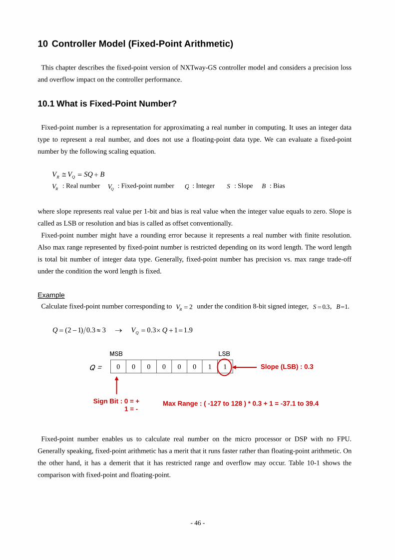
10.1 What is Fixed-Point Number?
Fixed-point number is a representation for approximating a real number in computing. It uses an integer data
type to represent a real number, and does not use a floating-point data type. We can evaluate a fixed-point
number by the following scaling equation.
V BSQV V : Real number : Fixed-point number R QV Q : Integer : Slope S B : Bias
where slope represents real value per 1-bit and bias is real value when the integer value equals to zero. Slope is
called as LSB or resolution and bias is called as offset conventionally.
Fixed-point number might have a rounding error because it represents a real number with finite resolution.
Also max range represented by fixed-point number is restricted depending on its word length. The word length
is total bit number of integer data type. Generally, fixed-point number has precision vs. max range trade-off
under the condition the word length is fixed.
Example Calculate fixed-point number corresponding to 2=RV under the condition 8-bit signed integer, , 3.0=S 1=B .
9.113.033.0)12( =+×=→≈−= QVQ Q
0 0 0 0 0 0 1 1
Sign Bit : 0 = + 1 = -
Slope (LSB) : 0.3
Max Range : ( -127 to 128 ) * 0.3 + 1 = -37.1 to 39.4
MSB LSB
Q =
Fixed-point number enables us to calculate real number on the micro processor or DSP with no FPU.
Generally speaking, fixed-point arithmetic has a merit that it runs faster rather than floating-point arithmetic. On
the other hand, it has a demerit that it has restricted range and overflow may occur. Table 10-1 shows the
comparison with fixed-point and floating-point.

- 47 -
Table 10-1 Fixed-Point vs. Floating-Point
Consideration Fixed-Point Floating-Point
Execution Speed Fast Slow
Hardware Power Consumption Low High
RAM / ROM Consumption Small Large
Word Size and Scaling Flexible Inflexible
Max Range Narrow Wide
Error Prone High Low
Development Time Long Short
10.2 Floating-Point to Fixed-Point Conversion
Fixed-Point Toolbox / Simulink Fixed Point enable the intrinsic fixed-point capabilities of the MATLAB /
Simulink product family. Refer the reference [3] to learn fixed-point modeling.
nxtway_gs_controller_fixpt.mdl is a fixed-point version of nxtway_gs_controller.mdl. It uses fixed-point data
types for wheel angle, body pitch angle, and battery variable instead of single precision data types. The key
points of fixed-point conversion are the following.
Fixed-Point Data Type
param_controller_fixpt.m defines Simulink.NumericType objects used in nxtway_gs_controller_fixpt.mdl.
Simulink.NumericType specifies any data types, for example, integer, floating-point, and fixed-point.
param_controller_fixpt.m% Fixed-Point Parameters % We can calculate how far NXTway-GS can move by using the following equation % >> double(intmax('int32')) * pi / 180 * R * S % where R is the wheel radius and S is the slope of dt_theta (S = 2^-14 etc.) % % S : Range [m] % 2^-10 : 1464.1 % 2^-14 : 91.5 % 2^-18 : 5.7 % 2^-22 : 0.36 % Simulink.NumericType for wheel angle % signed 32-bit integer, slope = 2^-14, bias = 0 dt_theta = fixdt(true, 32, 2^-14, 0); % Simulink.NumericType for body pitch angle % signed 32-bit integer, slope = 2^-20, bias = 0 dt_psi = fixdt(true, 32, 2^-20, 0); % Simulink.NumericType for battery % signed 32-bit integer, slope = 2^-17, bias = 0 dt_battery = fixdt(true, 32, 2^-17, 0);
- 48 -
Generally speaking, controller performance depends on data types used in it. There is trade-off between
precision and range in using same word length illustrated in 10.1 What is Fixed-Point Number?. It is
necessary for a controller designer to consider this trade-off in order to find best fixed-point settings.
In the case of NXTway-GS, the fixed-point settings for wheel angle and body pitch angle are important
because NXTway-GS cannot balance if a precision loss or overflow occurs. We can estimate how far
NXTway-GS can move by the following equation.
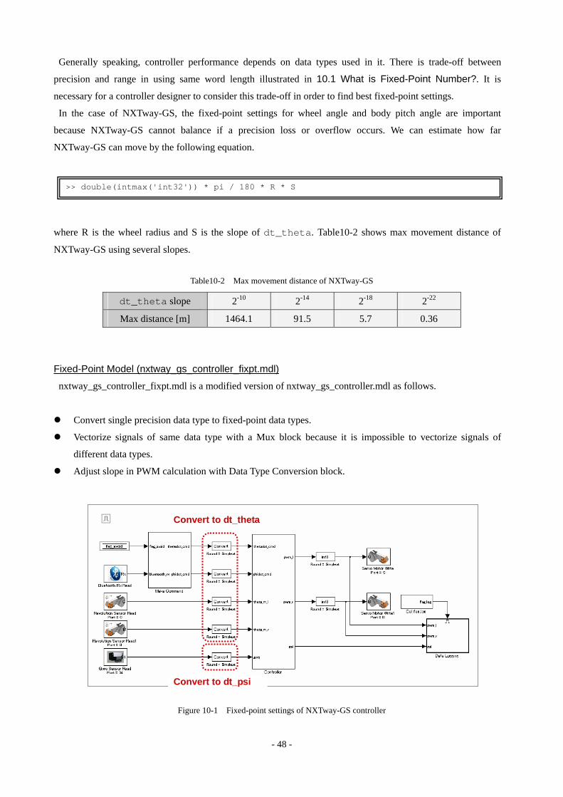
where R is the wheel radius and S is the slope of dt_theta. Table10-2 shows max movement distance of
NXTway-GS using several slopes.
Fixed-Point Model (nxtway_gs_controller_fixpt.mdl)
nxtway_gs_controller_fixpt.mdl is a modified version of nxtway_gs_controller.mdl as follows.
Convert single precision data type to fixed-point data types.
Vectorize signals of same data type with a Mux block because it is impossible to vectorize signals of
different data types.
Adjust slope in PWM calculation with Data Type Conversion block.
dt_theta slope 2-10 2-14 2-18 2-22
Max distance [m] 1464.1 91.5 5.7 0.36
>> double(intmax('int32')) * pi / 180 * R * S
Table10-2 Max movement distance of NXTway-GS
Convert to dt_theta
Convert to dt_psi
Figure 10-1 Fixed-point settings of NXTway-GS controller
- 49 -
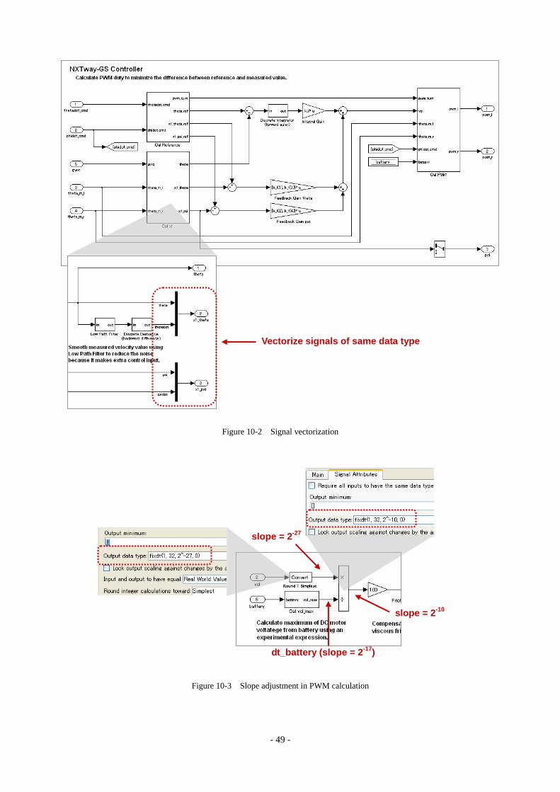
Vectorize signals of same data type
Figure 10-2 Signal vectorization
slope = 2-27
dt_battery (slope = 2-17)
slope = 2-10
Figure 10-3 Slope adjustment in PWM calculation
- 50 -
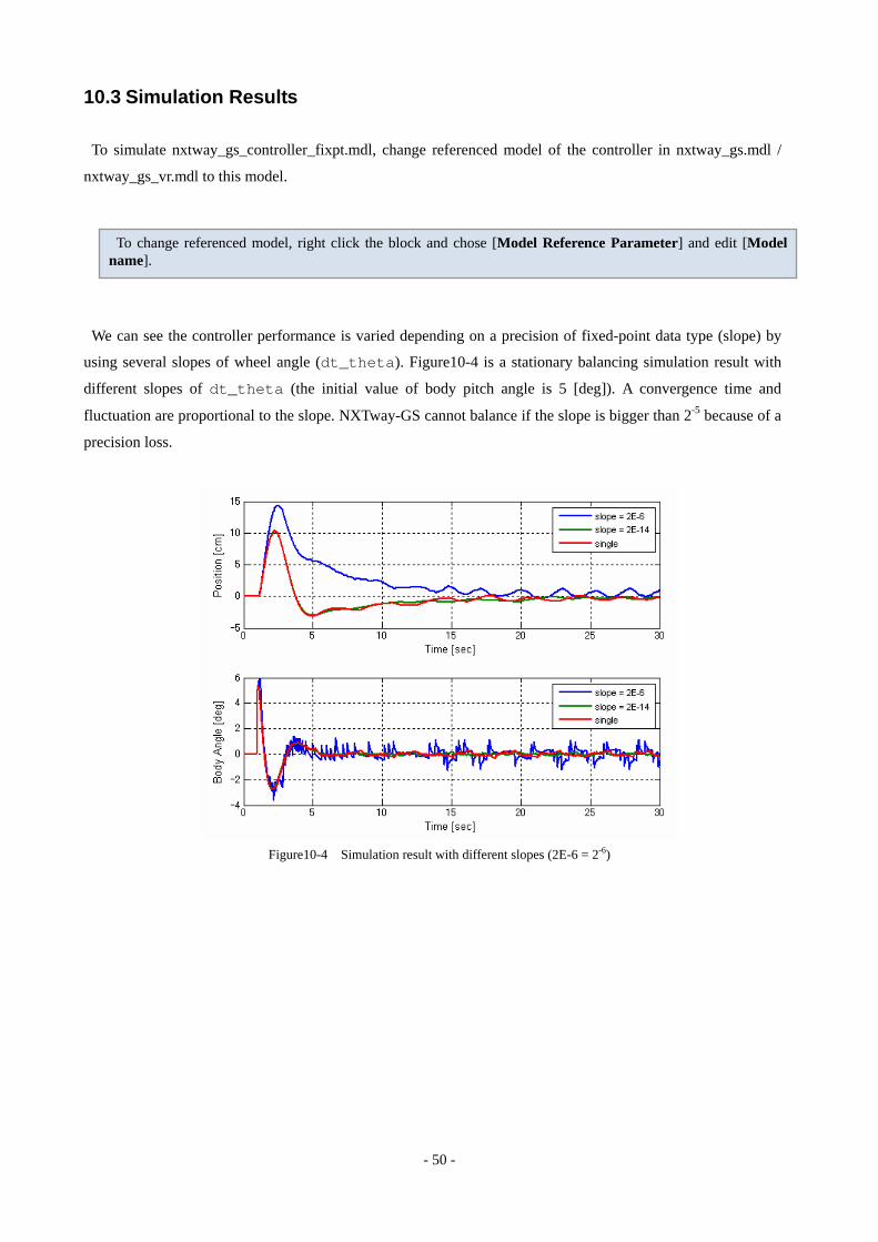
10.3 Simulation Results
To simulate nxtway_gs_controller_fixpt.mdl, change referenced model of the controller in nxtway_gs.mdl /
nxtway_gs_vr.mdl to this model.
To change referenced model, right click the block and chose [Model Reference Parameter] and edit [Model name].
We can see the controller performance is varied depending on a precision of fixed-point data type (slope) by
using several slopes of wheel angle (dt_theta). Figure10-4 is a stationary balancing simulation result with
different slopes of dt_theta (the initial value of body pitch angle is 5 [deg]). A convergence time and
fluctuation are proportional to the slope. NXTway-GS cannot balance if the slope is bigger than 2-5 because of a
precision loss.
Figure10-4 Simulation result with different slopes (2E-6 = 2-6)
- 51 -
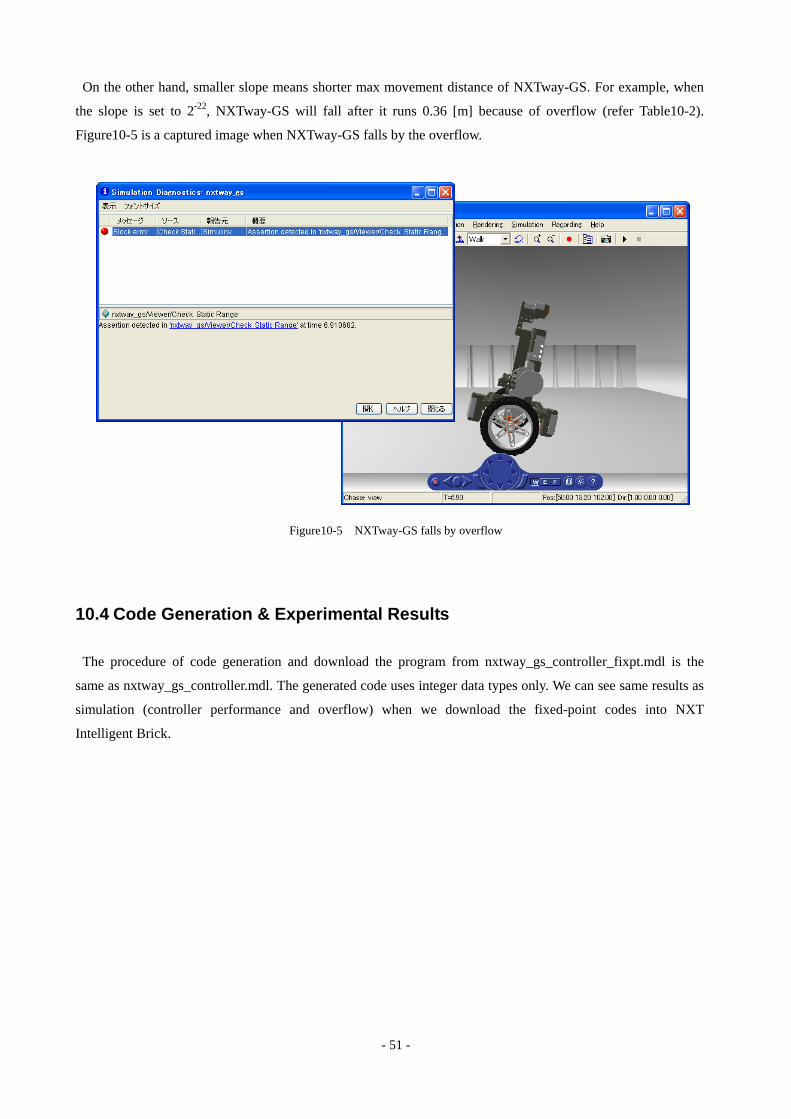
On the other hand, smaller slope means shorter max movement distance of NXTway-GS. For example, when
the slope is set to 2-22, NXTway-GS will fall after it runs 0.36 [m] because of overflow (refer Table10-2).
Figure10-5 is a captured image when NXTway-GS falls by the overflow.
Figure10-5 NXTway-GS falls by overflow
10.4 Code Generation & Experimental Results
The procedure of code generation and download the program from nxtway_gs_controller_fixpt.mdl is the
same as nxtway_gs_controller.mdl. The generated code uses integer data types only. We can see same results as
simulation (controller performance and overflow) when we download the fixed-point codes into NXT
Intelligent Brick.

- 52 -
11 Challenges for Readers
We provide the following problems as challenges for readers. Try them if you are interested in.
Controller performance improvement (gain tuning, robust control technique, etc.)
Use small wheels included in LEGO Mindstorms Education NXT Base Set.
Line tracing with a light sensor
Proportional sound to the distance between NXTway-GS and obstacle.
- 53 -
Appendix A Modern Control Theory
This appendix describes modern control theory used in controller design of NXTway-GS briefly. Refer
textbooks about control theory for more details.
A.1 Stability
We define a system is asymptotically stable when the state goes to zero independent of its initial value if the
input equals to zero. u
(A.1) 0)(lim =∞→
tt
x
A state equation is given as the following
(A.2) )()()( tBtAt uxx +=&
It is necessary and sufficient condition for asymptotically stable that the real part of all eigenvalues of system
matrix A is negative. The system is unstable when it has some eigenvalues with positive real part.
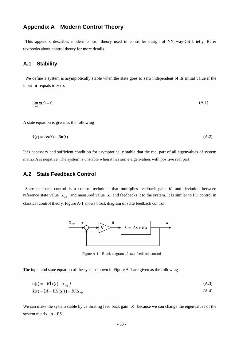
A.2 State Feedback Control
State feedback control is a control technique that multiplies feedback gain K and deviation between reference state value and measured value and feedbacks it to the system. It is similar to PD control in
classical control theory. Figure A-1 shows block diagram of state feedback control. refx x
The input and state equation of the system shown in Figure A-1 are given as the following
( )reftKt xxu −−= )()( (A.3)
(A.4) ( ) refBKtBKAt xxx +−= )()(&
We can make the system stable by calibrating feed back gain K because we can change the eigenvalues of the
system matrix BKA− .
uxx BA +=&u xrefx +
−K
Figure A-1 Block diagram of state feedback control
- 54 -
It is necessary to use state feedback control that the system is controllability. It is necessary and sufficient condition that a controllability matrix is full rank. (cM nMrank c =)( , is order of ) n x
[ ]BAABBM n
c1,, −= L (A.5)
Control System Toolbox provides ctrb function for evaluating a controllability matrix.
Example
Is the following system controllable? A = [0, 1; -2, -3], B = [0; 1] --> controllable
There are two methods to evaluate feedback gain K .
1. Direct Pole Placement
This method calculates feedback gain K so as to assign the poles (eigenvalues) of system matrix
BKA− at the desired positions. The tuning parameters are the poles and you need to decide appropriate
gain value by trial and error. Control System Toolbox provides place function for direct pole placement.
Example
Calculate feedback gain for the system A = [0, 1; -2, -3], B = [0; 1] so as to assign the poles in [-5, -6].
>> A = [0, 1; -2, -3]; B = [0; 1]; >> Mc = ctrb(A, B); >> rank(Mc) ans = 2
>> A = [0, 1; -2, -3]; B = [0; 1]; >> poles = [-5, -6]; >> K = place(A, B, poles) K = 28.0000 8.0000
2. Linear Quadratic Regulator
This method calculates feedback gain K so as to minimize the cost function given as the following
The tuning parameters are weight matrix for state and for input . You need to decide appropriate
gain value by trial and error. Control System Toolbox provides lqr function for linear quadratic regulator.
J
( )∫∞
+=0
)()()()( dttRttQtJ TT uuxx
Q R
- 55 -
Example
Calculate feedback gain for the system A = [0, 1; -2, -3], B = [0; 1] by using Q = [100, 0; 0, 1], R = 1.
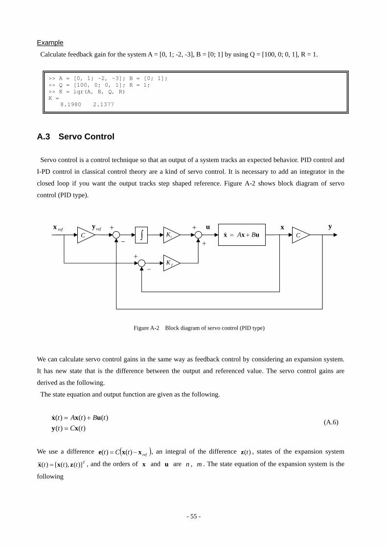
A.3 Servo Control
Servo control is a control technique so that an output of a system tracks an expected behavior. PID control and
I-PD control in classical control theory are a kind of servo control. It is necessary to add an integrator in the
closed loop if you want the output tracks step shaped reference. Figure A-2 shows block diagram of servo
control (PID type).
y
We can calculate servo control gains in the same way as feedback control by considering an expansion system.
It has new state that is the difference between the output and referenced value. The servo control gains are
derived as the following.
The state equation and output function are given as the following.
(A.6) )()(
)()()(tCt
tBtAtxy
uxx=
+=&
We use a difference ( )reftCt xxe −= )()( , an integral of the difference , states of the expansion system )(tz
Tttt )](),([)( zxx = , and the orders of and are , . The state equation of the expansion system is the
following
x u n m
uxx BA +=&u x+
+iK C
+∫C
refx refy
−
fK+
−
>> A = [0, 1; -2, -3]; B = [0; 1]; >> Q = [100, 0; 0, 1]; R = 1; >> K = lqr(A, B, Q, R) K = 8.1980 2.1377
Figure A-2 Block diagram of servo control (PID type)
- 56 -
(A.7) ref
mm
mn
mmmm
mn CI
tB
tt
CA
tt
xuzx
zx
⎥⎦
⎤⎢⎣
⎡−⎥
⎦
⎤⎢⎣
⎡+⎥
⎦
⎤⎢⎣
⎡⎥⎦
⎤⎢⎣
⎡=⎥
⎦
⎤⎢⎣
⎡
×
×
××
× 0)(
0)()(
00
)()(
&
&
Eq. (A.7) converges to Eq. (A.8) if the expansion system is assumed to be stable.
(A.8) ref
mm
mn
mmmm
mn CI
BCA
xuzx
zx
⎥⎦
⎤⎢⎣
⎡−∞⎥
⎦
⎤⎢⎣
⎡+⎥
⎦
⎤⎢⎣
⎡∞∞
⎥⎦
⎤⎢⎣
⎡=⎥
⎦
⎤⎢⎣
⎡∞∞
×
×
××
× 0)(
0)()(
00
)()(
&
&
The state equation (A.9) is derived by considering the subtraction between Eq. (A.7) and Eq. (A.8).
)()()()(0)(
)(00
)()(
tBtAtdtdt
Btt
CA
tt
eeeemme
e
mm
mn
e
e uxxuzx
zx
+=→⎥⎦
⎤⎢⎣
⎡+⎥
⎦
⎤⎢⎣
⎡⎥⎦
⎤⎢⎣
⎡=⎥
⎦
⎤⎢⎣
⎡
××
×
&
& (A.9)
where , )()( ∞−= xxx te )()( ∞−= zzz te , )()( ∞−= uuu te . We can use feedback control to make the
expansion system stable. The input is
)()()()( tKtKtKt eiefee zxxu −−=−= (A.10)
If it is possible that , , refxx →∞)( 0)( →∞z 0)( →∞u are assumed, we derive the following input . )(tu
(A.11) ( dttCKtKt refireff ∫ −−−−= xxxxu )())(()( )
Modern control theory textbooks usually describe I-PD type expression ( in the first term of Eq. (A.11) equals to zero) as servo control input. However we use PID type ex
refxpression Eq. (A.11) because of improving the
tracking performance.
- 57 -
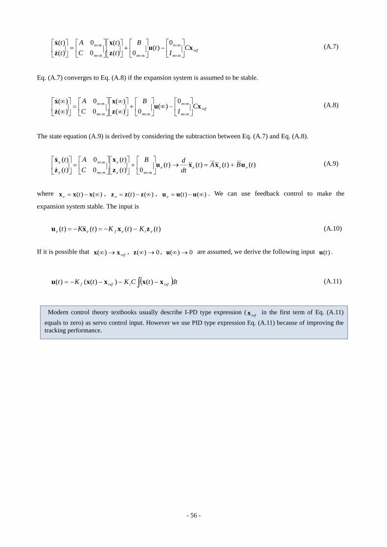
Appendix B Virtual Reality Space
This appendix describes the virtual reality space used in NXTway-GS model. For example, coordinate system,
map file, distance calculation, and wall hit detection.
B.1 Coordinate System
We use Virtual Reality Toolbox for 3D visualization of NXTway-GS. Virtual Reality Toolbox visualizes an
object based on VRML language. The VRML coordinate system is defined as shown in Figure B-1.
x
y
z
z
x
y
MATLAB Graphics VRML
Figure B-1 MATLAB and VRML coordinate system
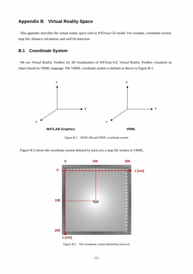
Figure B-2 shows the coordinate system defined by track.wrl, a map file written in VRML.
z [cm]
x [cm]
0 100 200
0
100
200
Figure B-2 The coordinate system defined by track.wrl
- 58 -
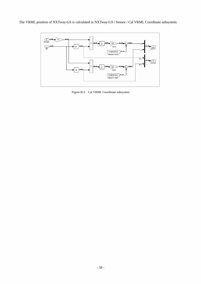
The VRML position of NXTway-GS is calculated in NXTway-GS / Sensor / Cal VRML Coordinate subsystem.
Figure B-3 Cal VRML Coordinate subsystem
- 59 -
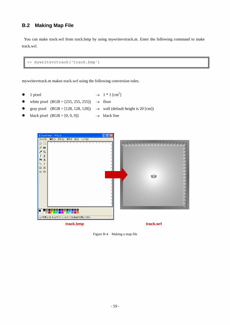
B.2 Making Map File
You can make track.wrl from track.bmp by using mywritevrtrack.m. Enter the following command to make
track.wrl.
>> mywritevrtrack('track.bmp')
mywritevrtrack.m makes track.wrl using the following conversion rules.
1 pixel 1 * 1 [cm→ 2]
white pixel (RGB = [255, 255, 255]) floor →
gray pixel (RGB = [128, 128, 128]) wall (default height is 20 [cm]) →
black pixel (RGB = [0, 0, 0]) black line →
track.bmp track.wrl
Figure B-4 Making a map file
- 60 -
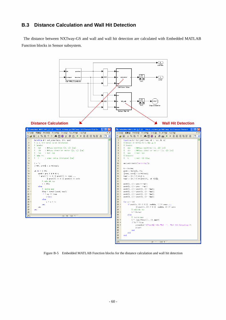
B.3 Distance Calculation and Wall Hit Detection
The distance between NXTway-GS and wall and wall hit detection are calculated with Embedded MATLAB
Function blocks in Sensor subsystem.
Distance Calculation Wall Hit Detection
Figure B-5 Embedded MATLAB Function blocks for the distance calculation and wall hit detection
- 61 -
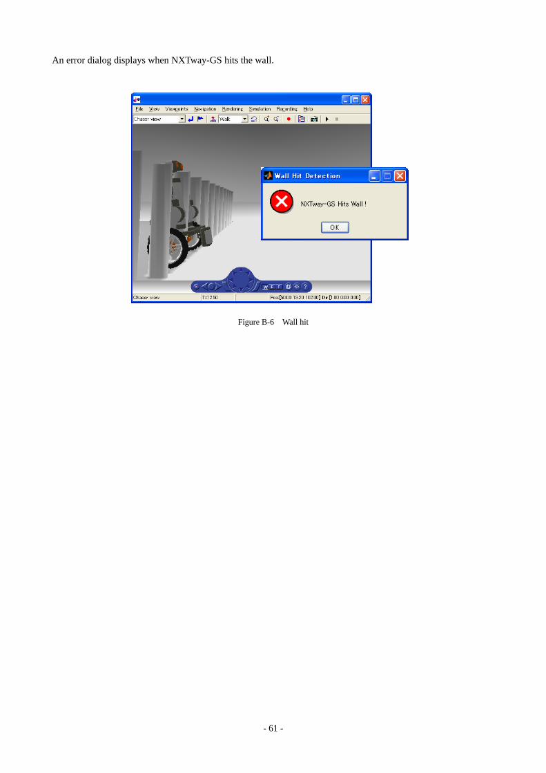
An error dialog displays when NXTway-GS hits the wall.
Figure B-6 Wall hit
- 62 -
Appendix C Generated Code
This appendix describes a main code generated from nxtway_gs_controller.mdl. It is a default code generated
by RTW-EC. RTW-EC allows us to assign user variable attributes such as variable name, storage class,
modifiers etc. by using Simulink Data Object, but we does not use it here. The comments are omitted for
compactness.
nxtway_app.c #include "nxtway_app.h" #include "nxtway_app_private.h" BlockIO rtB; D_Work rtDWork; void task_init(void) { rtDWork.battery = (real32_T)ecrobot_get_battery_voltage(); rtDWork.flag_mode = 0U; rtDWork.gyro_offset = (real32_T)ecrobot_get_gyro_sensor(NXT_PORT_S4); rtDWork.start_time = ecrobot_get_systick_ms(); } void task_ts1(void) { real32_T rtb_UnitDelay; real32_T rtb_IntegralGain; real32_T rtb_Sum_g; real32_T rtb_UnitDelay_j; real32_T rtb_Sum_a; real32_T rtb_UnitDelay_l; real32_T rtb_DataTypeConversion4; real32_T rtb_theta; real32_T rtb_Sum2_b[4]; real32_T rtb_Gain2_d; real32_T rtb_DataTypeConversion3; real32_T rtb_psidot; real32_T rtb_Sum_b; real32_T rtb_Saturation1; int16_T rtb_DataTypeConversion2_gl; int8_T rtb_DataTypeConversion; int8_T rtb_DataTypeConversion6; int8_T rtb_Switch; int8_T rtb_Switch2_e; int8_T rtb_DataTypeConversion_m[2]; uint8_T rtb_UnitDelay_lv; boolean_T rtb_DataStoreRead; boolean_T rtb_DataStoreRead1; boolean_T rtb_Switch3_m; { int32_T i; rtb_DataStoreRead = rtDWork.flag_start; if (rtDWork.flag_start) { rtb_UnitDelay = rtDWork.UnitDelay_DSTATE; rtb_IntegralGain = -4.472135901E-001F * rtDWork.UnitDelay_DSTATE; rtb_UnitDelay_l = rtDWork.UnitDelay_DSTATE_j; rtb_DataStoreRead1 = rtDWork.flag_avoid; if (rtDWork.flag_mode) { if (rtDWork.flag_auto) { if (rtDWork.flag_avoid) { rtb_Switch = 0; } else { rtb_Switch = 100;
- 63 -
} if (rtDWork.flag_avoid) { rtb_Switch2_e = 100; } else { rtb_Switch2_e = 0; } } else { rtb_Switch = 0; rtb_Switch2_e = 0; } } else { ecrobot_read_bt_packet(rtB.BluetoothRxRead, 32); for (i = 0; i < 2; i++) { rtb_DataTypeConversion_m[i] = (int8_T)rtB.BluetoothRxRead[i]; } if (rtb_DataStoreRead1) { rtb_Switch = 100; } else { rtb_Switch = rtb_DataTypeConversion_m[0]; } rtb_Switch = (int8_T)(-rtb_Switch); rtb_Switch2_e = rtb_DataTypeConversion_m[1]; } rtb_Sum_g = (real32_T)rtb_Switch / 100.0F * 7.5F * 4.000000190E-003F + 9.959999919E-001F * rtDWork.UnitDelay_DSTATE_e; rtb_DataTypeConversion3 = (real32_T)ecrobot_get_motor_rev(NXT_PORT_C); rtb_UnitDelay_j = rtDWork.UnitDelay_DSTATE_h; rtb_DataTypeConversion4 = (real32_T)ecrobot_get_motor_rev(NXT_PORT_B); rtb_theta = ((1.745329238E-002F * rtb_DataTypeConversion3 + rtDWork.UnitDelay_DSTATE_h) + (1.745329238E-002F * rtb_DataTypeConversion4 + rtDWork.UnitDelay_DSTATE_h)) / 2.0F; rtb_Sum_a = 2.000000030E-001F * rtb_theta + 8.000000119E-001F * rtDWork.UnitDelay_DSTATE_hp; rtb_Sum_b = (real32_T)ecrobot_get_gyro_sensor(NXT_PORT_S4); rtDWork.gyro_offset = 9.990000129E-001F * rtDWork.gyro_offset + 1.000000047E-003F * rtb_Sum_b; rtb_psidot = (rtb_Sum_b - rtDWork.gyro_offset) * 1.745329238E-002F; rtb_Sum2_b[0] = rtb_UnitDelay_l - rtb_theta; rtb_Sum2_b[1] = 0.0F - rtDWork.UnitDelay_DSTATE_h; rtb_Sum2_b[2] = rtb_Sum_g - (rtb_Sum_a - rtDWork.UnitDelay_DSTATE_m) / 4.000000190E-003F; rtb_Sum2_b[3] = 0.0F - rtb_psidot; { static const int_T dims[3] = { 1, 4, 1 }; rt_MatMultRR_Sgl((real32_T *)&rtb_Sum_b, (real32_T *) &rtConstP.FeedbackGain_Gain[0], (real32_T *)rtb_Sum2_b, &dims[0]); } rtb_IntegralGain += rtb_Sum_b; rtb_Sum_b = rtDWork.battery; rtb_Sum_b = rtb_IntegralGain / (1.089000027E-003F * rtb_Sum_b - 0.625F) * 100.0F; rtb_Sum_b += 0.0F * rt_FSGN(rtb_Sum_b); rtb_IntegralGain = (real32_T)rtb_Switch2_e; rtb_Gain2_d = rtb_IntegralGain / 100.0F * 25.0F; rtb_Saturation1 = rtb_Sum_b + rtb_Gain2_d; rtb_Saturation1 = rt_SATURATE(rtb_Saturation1, -100.0F, 100.0F); rtb_DataTypeConversion = (int8_T)rtb_Saturation1; ecrobot_set_motor_speed(NXT_PORT_C, rtb_DataTypeConversion); if ((int8_T)rtb_IntegralGain != 0) { rtb_DataStoreRead1 = 1U; } else { rtb_DataStoreRead1 = 0U;
- 64 -
} rtb_IntegralGain = rtb_DataTypeConversion3 - rtb_DataTypeConversion4; if ((!rtb_DataStoreRead1) && rtDWork.UnitDelay_DSTATE_c) { rtB.theta_diff = rtb_IntegralGain; } if (rtb_DataStoreRead1) { rtb_Saturation1 = 0.0F; } else { rtb_Saturation1 = (rtb_IntegralGain - rtB.theta_diff) *
3.499999940E-001F; } rtb_Saturation1 += rtb_Sum_b - rtb_Gain2_d; rtb_Saturation1 = rt_SATURATE(rtb_Saturation1, -100.0F, 100.0F);
rtb_DataTypeConversion6 = (int8_T)rtb_Saturation1; ecrobot_set_motor_speed(NXT_PORT_B, rtb_DataTypeConversion6);
rtb_UnitDelay_lv = rtDWork.UnitDelay_DSTATE_k; if (rtDWork.UnitDelay_DSTATE_k != 0U) { rtb_Switch3_m = 0U; } else { rtb_Switch3_m = 1U;
}
if (rtb_Switch3_m) { rtb_DataTypeConversion2_gl = (int16_T)floor((real_T)(5.729578018E+001F * rtb_UnitDelay_j / 0.0009765625F) + 0.5); ecrobot_bt_adc_data_logger(rtb_DataTypeConversion, rtb_DataTypeConversion6, rtb_DataTypeConversion2_gl, 0, 0, 0);
}
rtb_UnitDelay_lv = (uint8_T)(1U + (uint32_T)rtb_UnitDelay_lv); if (25U == rtb_UnitDelay_lv) { rtDWork.UnitDelay_DSTATE_k = 0U; } else { rtDWork.UnitDelay_DSTATE_k = rtb_UnitDelay_lv;
}
rtDWork.UnitDelay_DSTATE = (rtb_UnitDelay_l - rtb_theta) * 4.000000190E-003F + rtb_UnitDelay; rtDWork.UnitDelay_DSTATE_j = 4.000000190E-003F * rtb_Sum_g + rtb_UnitDelay_l; rtDWork.UnitDelay_DSTATE_e = rtb_Sum_g; rtDWork.UnitDelay_DSTATE_h = 4.000000190E-003F * rtb_psidot + rtb_UnitDelay_j;
rtDWork.UnitDelay_DSTATE_hp = rtb_Sum_a; rtDWork.UnitDelay_DSTATE_m = rtb_Sum_a;
rtDWork.UnitDelay_DSTATE_c = rtb_DataStoreRead1; } if (!rtb_DataStoreRead) { rtDWork.gyro_offset = 8.000000119E-001F * rtDWork.gyro_offset +
2.000000030E-001F * (real32_T)ecrobot_get_gyro_sensor(NXT_PORT_S4); }
} } void task_ts2(void) {
boolean_T rtb_DataStoreRead2_j; if (rtDWork.flag_mode) {
rtb_DataStoreRead2_j = rtDWork.flag_avoid; if (!rtDWork.flag_avoid) { rtDWork.flag_avoid = (ecrobot_get_sonar_sensor(NXT_PORT_S2) <= 20); rtB.RevolutionSensor_C = ecrobot_get_motor_rev(NXT_PORT_C); } if (rtb_DataStoreRead2_j) {
rtDWork.flag_avoid = (ecrobot_get_motor_rev(NXT_PORT_C) -
- 65 -
rtB.RevolutionSensor_C <= 210); }
} if (!rtDWork.flag_mode) { rtDWork.flag_avoid = (ecrobot_get_sonar_sensor(NXT_PORT_S2) <= 20); }
}
void task_ts3(void) { uint32_T rtb_Sum1_i; boolean_T rtb_RelationalOperator_e0; rtDWork.battery = 8.000000119E-001F * rtDWork.battery + 2.000000030E-001F * (real32_T)ecrobot_get_battery_voltage(); rtb_Sum1_i = (uint32_T)((int32_T)ecrobot_get_systick_ms() - (int32_T)
rtDWork.start_time); rtb_RelationalOperator_e0 = (rtb_Sum1_i >= 1000U);
rtDWork.flag_start = rtb_RelationalOperator_e0; rtDWork.flag_auto = (rtb_Sum1_i >= 5000U); if (rtb_RelationalOperator_e0 != rtDWork.UnitDelay_DSTATE_a) { sound_freq(440U, 500U); }
rtDWork.UnitDelay_DSTATE_a = rtb_RelationalOperator_e0;
} void nxtway_app_initialize(void) { }

- 66 -
References
[1] Philo’s Home Page LEGO Mindstorms NXT
http://www.philohome.com/
[2] Ryo’s Holiday LEGO Mindstorms NXT
http://web.mac.com/ryo_watanabe/iWeb/Ryo%27s%20Holiday/LEGO%20Mindstorms%20NXT.html
[3] Tips for Fixed-Point Modeling and Code Generation for Simulink 6
http://www.mathworks.com/matlabcentral/fileexchange/7197


![AVR - dl.melec.irdl.melec.ir/download/pdf/AVR/CodeVision-Fusebit[Melec.ir].pdf · AVR AVR AVR AVR 01 CodeVision CKSEL3..0 Device Clocking Option CKSEL3..0 External Crystal/Ceramic](https://img.pdfslide.us/doc/110x75/5cf6e10d88c99387248bfc0e/avr-dlmelecirdlmelecirdownloadpdfavrcodevision-fusebitmelecirpdf.jpg)