nWP-017 Antenna tuning White paper v1.0infocenter.nordicsemi.com/pdf/nwp_017.pdf · Page 3 of 38 White Paper - Antenna Tuning v1.0 1 Antenna resonance explained The capacitance and

Copyright © 2012 Nordic Semiconductor ASA. All rights reserved.Reproduction in whole or in part is prohibited without the prior written permission of the copyright holder.

Antenna tuning

nWP-017

White Paper v1.0

The antenna is an important component in any radio design. This means that it is very important to tune the antenna correctly to achieve the best performance for the radio. If the antenna is not correctly tuned, a lot of transmitter power is lost, the operating range is shortened and, interference problems increase.

This white paper explains how to tune an antenna and subsequently improve radio communication range.

White Paper - Antenna Tuning v1.0

Table of contents1 Antenna resonance explained ............................................................................................................... 3

2 Why tune the antenna? ........................................................................................................................... 4

3 Smith chart explained.............................................................................................................................. 53.1 The Resistance circles and the Reactance arcs ...................................................................................... 63.2 The Conductance circles and the Susceptance arcs............................................................................ 73.3 Moving the impedance point ...................................................................................................................... 8

4 Methods of tuning an antenna ............................................................................................................ 114.1 Length adjustment and a single component ......................................................................................114.2 Pi-network.........................................................................................................................................................13

5 Calculating the component values ..................................................................................................... 155.1 Adding a series capacitor ............................................................................................................................155.2 Adding a shunt capacitor ............................................................................................................................175.3 Using more than one component............................................................................................................18

6 Non-ideal components.......................................................................................................................... 226.1 Capacitors..........................................................................................................................................................226.2 Inductors............................................................................................................................................................23

7 Equipment needed to tune an antenna ............................................................................................. 25

8 Examples .................................................................................................................................................. 268.1 Chip antenna....................................................................................................................................................268.2 PCB antenna .....................................................................................................................................................33

Page 2 of 38


1 Antenna resonance explainedThe capacitance and inductance of an antenna is determined by its physical properties and its environment. The most important parameter for the antenna resonance is the length. A long antenna resonates at a lower frequency than a shorter antenna because the wavelength decreases when the frequency increases. This means the length of the antenna is directly proportional to the frequency and the wavelength.

Since an antenna is designed around a resonant frequency, its bandwidth is limited to that specific resonant frequency. For example, an antenna designed for 900 MHz cannot be used at 2.4 GHz.

The capacitance and inductance can be changed either by changing the length, or by using external components, inductors, or capacitors.

An antenna with a different impedance from the system impedance (an un-tuned antenna) reflects some of the RF power back into the transmitter. The reflected power is lost in the tuning network or the power amplifier. The ratio between the power absorbed by the antenna and the reflected power is called Standing Wave Ratio (SWR). Perfect radiation of the power gives an SWR = 1.0 and increasing numbers means more reflected power. This can be measured with an SWR meter or a network analyzer.

An antenna needs to resonate at the operating frequency to maximize its radiation. The resonance frequency is where the impedance of the inductance XL equals the impedance of the capacitance XC. So at the resonance frequency the antenna appears purely resistive. The resistance is a combination of loss resistance and radiation resistance. For an optimized system, the impedance seen into the antenna should match the characteristic impedance (system impedance), which is normally 50 ohm.

Page 3 of 38


2 Why tune the antenna?The efficiency and radiation pattern of an antenna depends on:

• Size and shape of the antenna element• The housing• Proximity to metal• Shape and size of the ground plane

A single-ended monopole antenna works together with the ground plane to form a dipole antenna. Consequently, the ground plane can be described as the ‘second half’ of the antenna.

This means that even if the antenna performs well in one application, it will almost never get the same performance in another application. Therefore, a cut-and-paste approach is not recommended. The antenna needs to be adapted to different applications.

An un-tuned antenna has less efficiency than a tuned antenna. Higher efficiency means more radiated power and increased operation range. For optimum performance, the antenna has to be tuned to increase the operation range.

Page 4 of 38


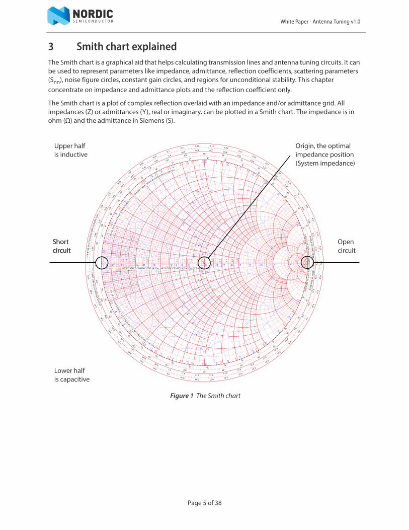
3 Smith chart explainedThe Smith chart is a graphical aid that helps calculating transmission lines and antenna tuning circuits. It can be used to represent parameters like impedance, admittance, reflection coefficients, scattering parameters (Snn), noise figure circles, constant gain circles, and regions for unconditional stability. This chapter concentrate on impedance and admittance plots and the reflection coefficient only.

The Smith chart is a plot of complex reflection overlaid with an impedance and/or admittance grid. All impedances (Z) or admittances (Y), real or imaginary, can be plotted in a Smith chart. The impedance is in ohm (Ω) and the admittance in Siemens (S).

Figure 1 The Smith chart

0.1

0.1

0.2

0.2

0.2

0.3

0.3

0.4

0.4

0.4

0.50.5

0.5

0.60.6

0.6

0.70.7

0.7

0.80.8

0.80.9

0.9

0.9

1.01.0

1.0

1.21.2

1.2

1.41.4

1.4

1.61.6

1.6

1.81.8

1.8

2.02.0

2.0

3.0

3.0

3.0

4.0

4.0

4.0

5.0

5.0

5.0

10

10

10

20

20

20

50

50

50

0.2

0.2

0.2

0.2

0.4

0.4

0.4

0.4

0.6

0.6

0.6

0.6

0.8

0.8

0.8

0.8

1.0

1.0

1.01.0

0.10.1

0.1

0.20.2

0.2

0.30.3

0.3

0.40.4

0.4

0.50.5

0.5

0.60.6

0.6

0.70.7

0.70.8

0.8

0.80.9

0.9

0.9

1.01.0

1.0

1.21.2

1.2

1.41.4

1.4

1.61.6

1.6

1.81.8

1.8

2.02.0

2.0

3.03.0

3.0

4.04.0

4.0

5.05.0

5.0

10

10

2020

20

5050

50

0.20.2

0.20.2

0.40.4

0.40.4

0.60.6

0.60.6

0.80.8

0.80.8

1.01.0

1.01.0

20-20

30-30

40-40

50

-50

60

-60

70

-70

80

-80

90-90

100-100

110-110

120-120

130-130

140-14

0

150

-150

160

-160

170

-170

180

±

90-9

085

-85

80-8

0

75-7

5

70-7

0

65-65

60-60

55-55

50-50

45

-45

40-40

35-35

30-30

25-25

20-20

15-15

10-10

0.04

0.04

0.05

0.05

0.06

0.06

0.07

0.070.08

0.080.09

0.090.1

0.1

0.11

0.11

0.12

0.12

0.13

0.13

0.14

0.14

0.15

0.15

0.16

0.16

0.17

0.17

0.18

0.18

0.190.19

0.20.2

0.210.21

0.220.22

0.230.23

0.240.24

0.25

0.25

0.26

0.26

0.27

0.27

0.28

0.28

0.29

0.29

0.30.3

0.310.31

0.320.32

0.330.33

0.340.34

0.350.35

0.360.36

0.370.370.38

0.380.39

0.390.4

0.4

0.410.41

0.420.42

0.430.43

0.44

0.44

0.45

0.45

0.46

0.46

0.47

0.47

0.48

0.48

0.49

0.49

00

ANGLE

OFTRAN

SMISS

ON

COEFFICIEN

TIN

DEGREES

ANGLE

OFREFLECTIO

NCO

EFFCIEN

TIN

DEGREES

—>

WAV

ELEN

GTH

S TOW

ARD

G EN

ERAT

OR—

><—

WAV

ELEN

GTH

STOW

ARD

LOAD

<—

INDU

CTIV

ERE

ACTA

NCECOMPO

NENT (+jX/Zo), O

R CAPACITIVE SUSCEPTANCE (+jB/Yo)

EACTANCECOMPONENT (-jX/Zo),

ORINDUCTI

VESU

SCEP

TANC

E(-j

BYo

)

RESISTANCE COMPONENT (R/Zo), OR CONDUCTANCE COMPONENT (G/Yo)

ShortcircuitShortcircuit

Opencircuit

Upper halfis inductive

Lower halfis capacitive

Origin, the optimalimpedance position(System impedance)

Page 5 of 38


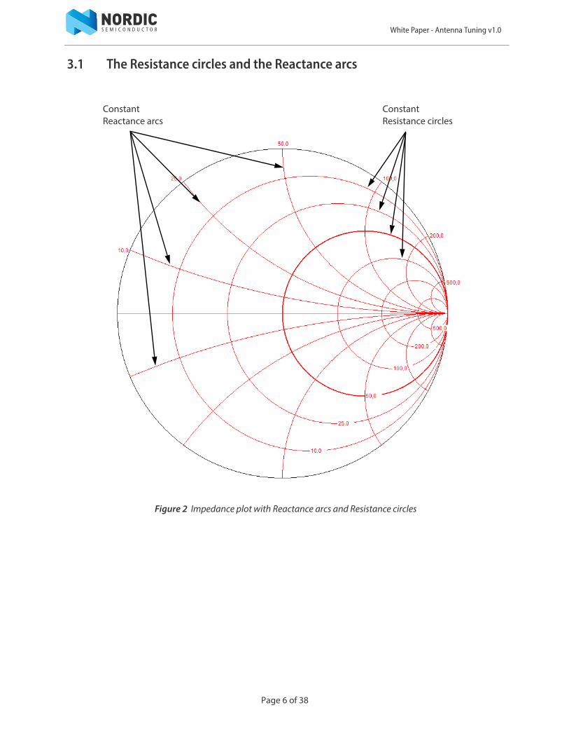
3.1 The Resistance circles and the Reactance arcs

Figure 2 Impedance plot with Reactance arcs and Resistance circles

ConstantReactance arcs

ConstantResistance circles

Page 6 of 38


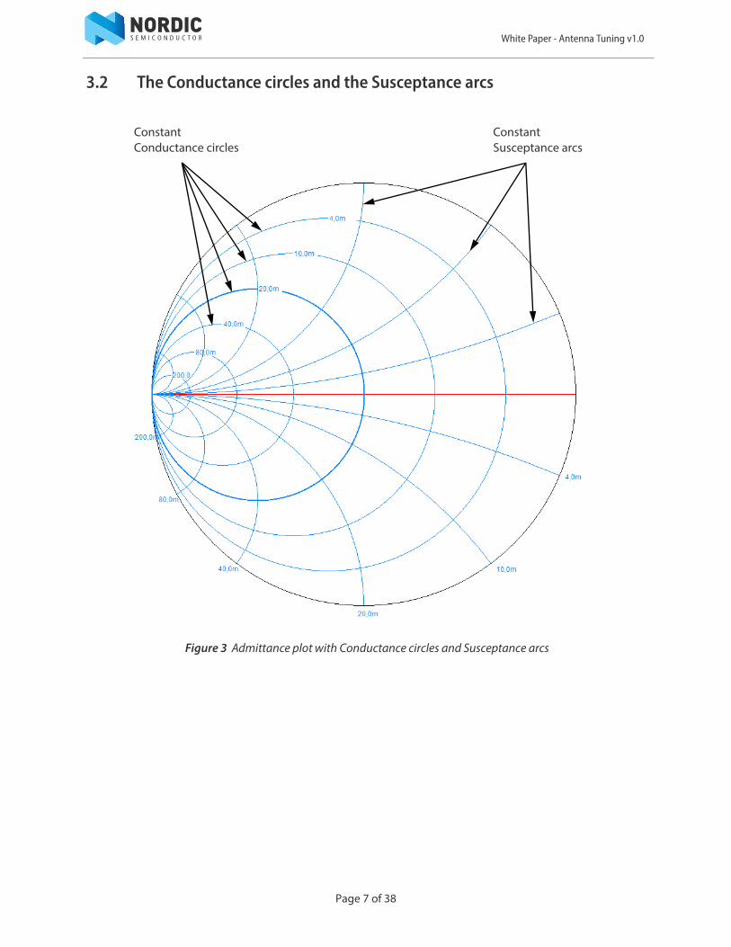
3.2 The Conductance circles and the Susceptance arcs

Figure 3 Admittance plot with Conductance circles and Susceptance arcs

ConstantConductance circles

ConstantSusceptance arcs

Page 7 of 38


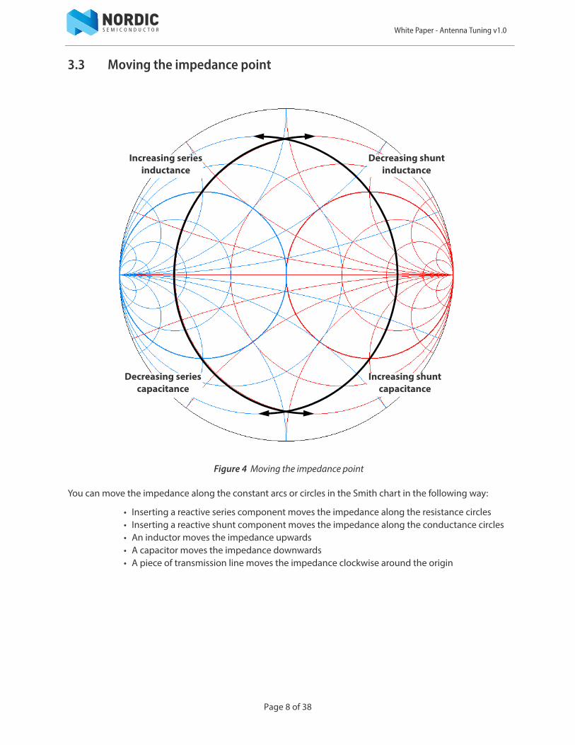
3.3 Moving the impedance point

Figure 4 Moving the impedance point

You can move the impedance along the constant arcs or circles in the Smith chart in the following way:

• Inserting a reactive series component moves the impedance along the resistance circles • Inserting a reactive shunt component moves the impedance along the conductance circles• An inductor moves the impedance upwards • A capacitor moves the impedance downwards• A piece of transmission line moves the impedance clockwise around the origin

Increasing seriesinductance

Decreasing shuntinductance

Decreasing seriescapacitance

Increasing shuntcapacitance

Page 8 of 38


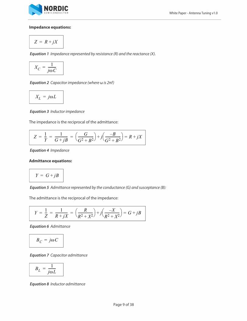
Impedance equations:

Equation 1 Impedance represented by resistance (R) and the reactance (X).

Equation 2 Capacitor impedance (where ω is 2πf)

Equation 3 Inductor impedance

The impedance is the reciprocal of the admittance:

Equation 4 Impedance

Admittance equations:

Equation 5 Admittance represented by the conductance (G) and susceptance (B):

The admittance is the reciprocal of the impedance:

Equation 6 Admittance

Equation 7 Capacitor admittance

Equation 8 Inductor admittance

Z R jX+=

XC1jC----------=

XL jL=

Z1Y--- 1

G jB+---------------- G

G2 B2+------------------- j

B–G2 B2+------------------- R jX+=+= = =

Y G jB+=

Y1Z--- 1

R jX+--------------- R

R2 X2+------------------ j

X–R2 X2+------------------ G jB+=+= = =

BC jC=

BL1jL---------=

Page 9 of 38


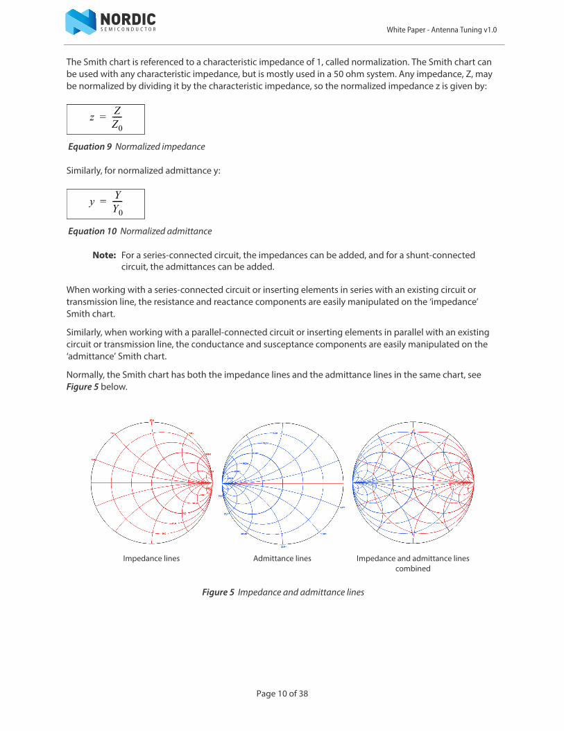
The Smith chart is referenced to a characteristic impedance of 1, called normalization. The Smith chart can be used with any characteristic impedance, but is mostly used in a 50 ohm system. Any impedance, Z, may be normalized by dividing it by the characteristic impedance, so the normalized impedance z is given by:

Equation 9 Normalized impedance

Similarly, for normalized admittance y:

Equation 10 Normalized admittance

Note: For a series-connected circuit, the impedances can be added, and for a shunt-connected circuit, the admittances can be added.

When working with a series-connected circuit or inserting elements in series with an existing circuit or transmission line, the resistance and reactance components are easily manipulated on the ‘impedance’ Smith chart.

Similarly, when working with a parallel-connected circuit or inserting elements in parallel with an existing circuit or transmission line, the conductance and susceptance components are easily manipulated on the ‘admittance’ Smith chart.

Normally, the Smith chart has both the impedance lines and the admittance lines in the same chart, see Figure 5 below.

Figure 5 Impedance and admittance lines

Impedance lines Admittance lines Impedance and admittance lines combined

zZZ0-----=

yYY0-----=

Page 10 of 38


4 Methods of tuning an antenna There are the following two methods to tune an antenna:

• If the physical dimensions of the antenna can be altered, for example, with a PCB antenna, adjusting the length will be one part of the tuning. Another part is to add a component, inductor, or capacitor, to pull the antenna impedance towards the 50 ohm center point.

• If the antenna cannot be altered physically, more external components must be used to tune the antenna. These external components are called the matching network.

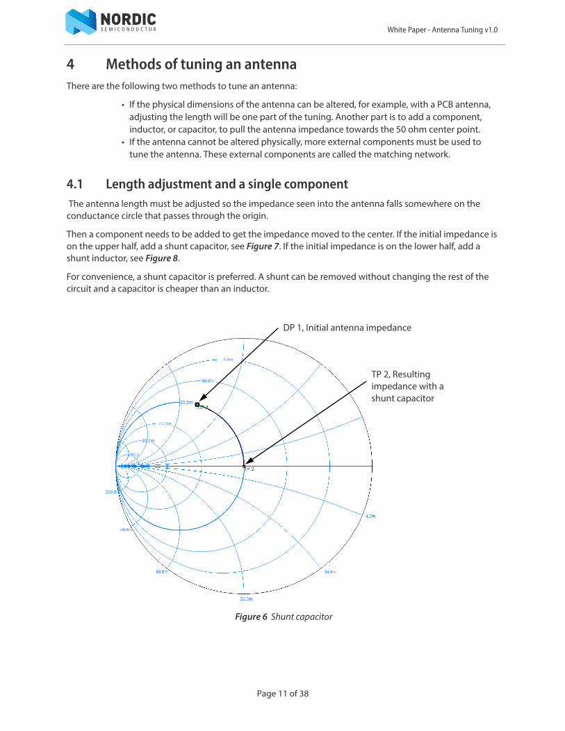
4.1 Length adjustment and a single component The antenna length must be adjusted so the impedance seen into the antenna falls somewhere on the conductance circle that passes through the origin.

Then a component needs to be added to get the impedance moved to the center. If the initial impedance is on the upper half, add a shunt capacitor, see Figure 7. If the initial impedance is on the lower half, add a shunt inductor, see Figure 8.

For convenience, a shunt capacitor is preferred. A shunt can be removed without changing the rest of the circuit and a capacitor is cheaper than an inductor.

Figure 6 Shunt capacitor

DP 1, Initial antenna impedance

TP 2, Resulting impedance with a shunt capacitor

Page 11 of 38


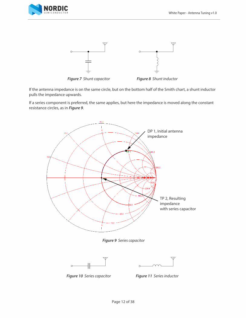
If the antenna impedance is on the same circle, but on the bottom half of the Smith chart, a shunt inductor pulls the impedance upwards.

If a series component is preferred, the same applies, but here the impedance is moved along the constant resistance circles, as in Figure 9.

Figure 9 Series capacitor

Figure 7 Shunt capacitor Figure 8 Shunt inductor

Figure 10 Series capacitor Figure 11 Series inductor

DP 1, Initial antenna impedance

TP 2, Resulting impedancewith series capacitor

Page 12 of 38


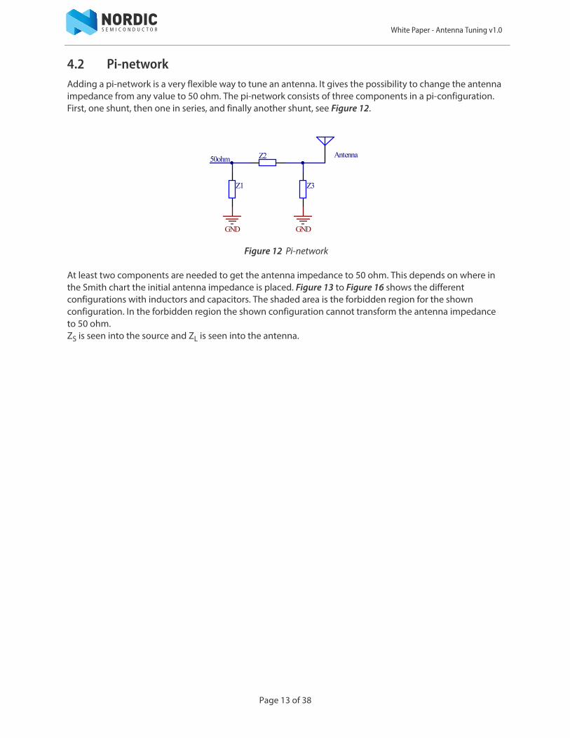
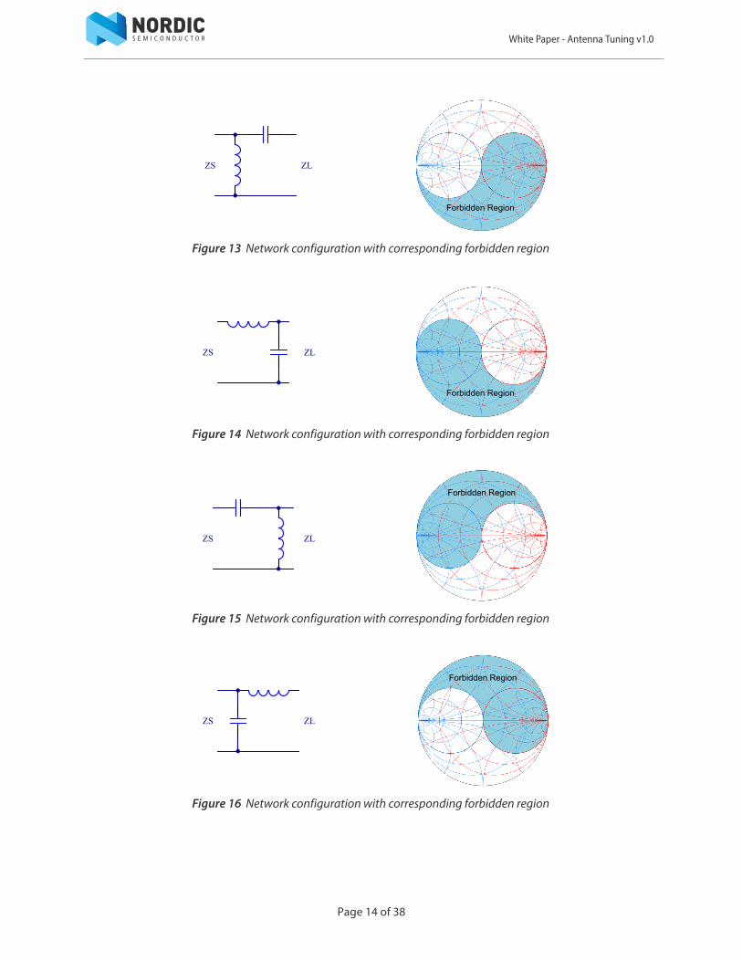
4.2 Pi-network Adding a pi-network is a very flexible way to tune an antenna. It gives the possibility to change the antenna impedance from any value to 50 ohm. The pi-network consists of three components in a pi-configuration. First, one shunt, then one in series, and finally another shunt, see Figure 12.

Figure 12 Pi-network

At least two components are needed to get the antenna impedance to 50 ohm. This depends on where in the Smith chart the initial antenna impedance is placed. Figure 13 to Figure 16 shows the different configurations with inductors and capacitors. The shaded area is the forbidden region for the shown configuration. In the forbidden region the shown configuration cannot transform the antenna impedance to 50 ohm. ZS is seen into the source and ZL is seen into the antenna.

Z2

Z1 Z3

GND GND

Antenna50ohm

Page 13 of 38


Figure 13 Network configuration with corresponding forbidden region




ZS ZL

Forbidden Region

ZS ZL

Forbidden Region

ZS ZL

Forbidden Region

ZS ZL

Forbidden Region

Page 14 of 38


5 Calculating the component valuesThis chapter describes how to calculate the values on the capacitors and/or inductors needed for antenna tuning.

The examples in Section 5.1, section 5.2 on page 17, and section 5.3 on page 18 explain how to calculate the values.

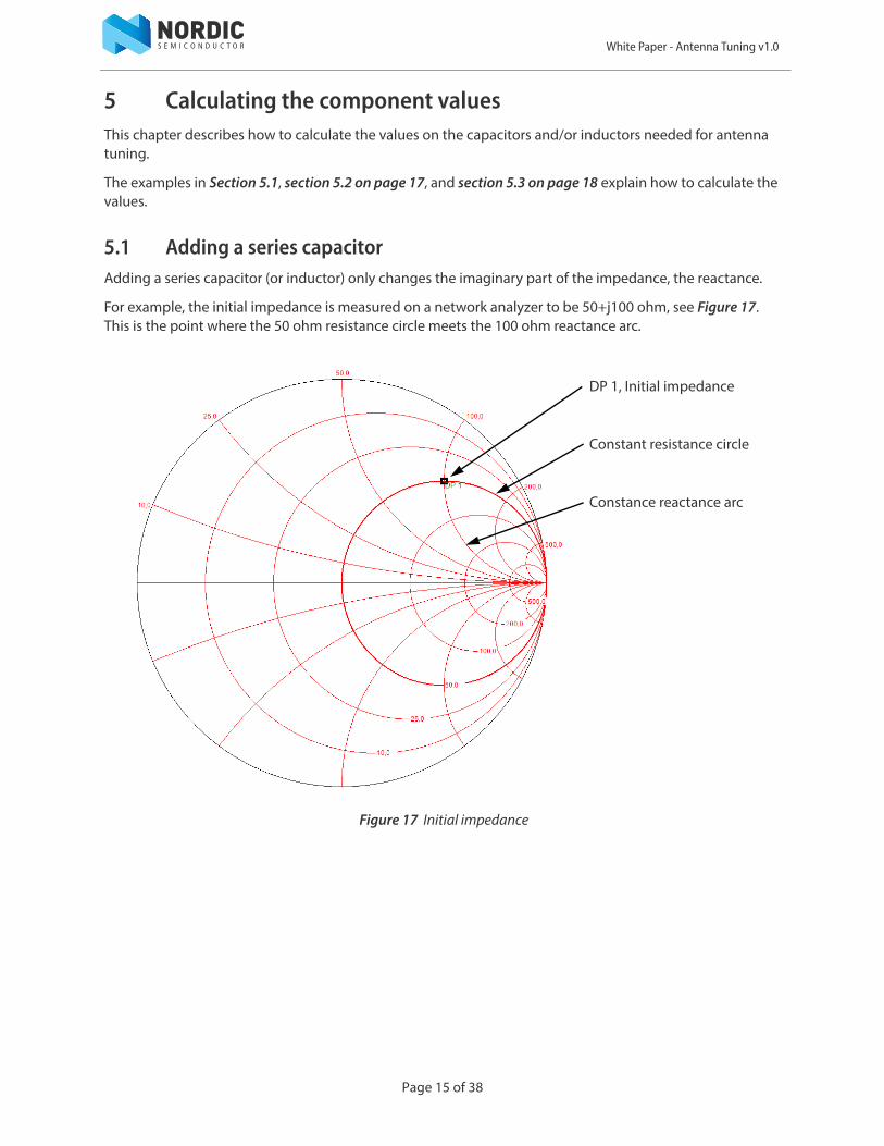
5.1 Adding a series capacitorAdding a series capacitor (or inductor) only changes the imaginary part of the impedance, the reactance.

For example, the initial impedance is measured on a network analyzer to be 50+j100 ohm, see Figure 17. This is the point where the 50 ohm resistance circle meets the 100 ohm reactance arc.

Figure 17 Initial impedance

DP 1, Initial impedance

Constant resistance circle

Constance reactance arc

Page 15 of 38


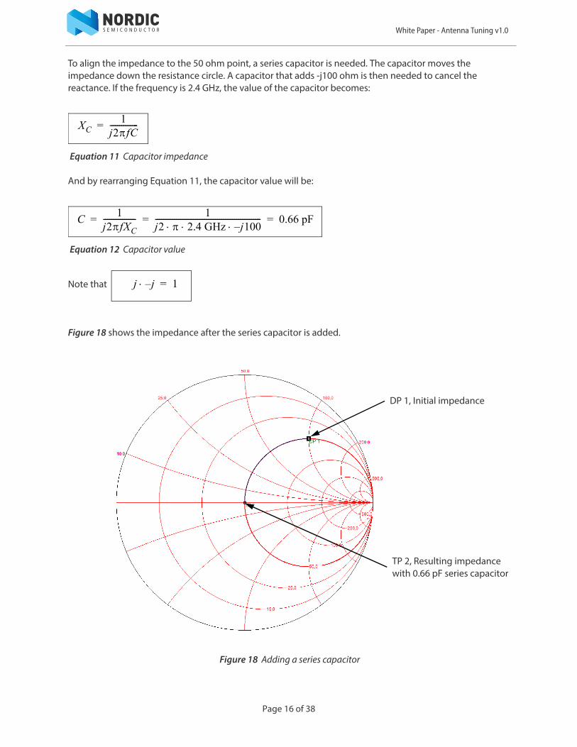
To align the impedance to the 50 ohm point, a series capacitor is needed. The capacitor moves the impedance down the resistance circle. A capacitor that adds -j100 ohm is then needed to cancel the reactance. If the frequency is 2.4 GHz, the value of the capacitor becomes:

Equation 11 Capacitor impedance

And by rearranging Equation 11, the capacitor value will be:

Equation 12 Capacitor value

Note that

Figure 18 shows the impedance after the series capacitor is added.

Figure 18 Adding a series capacitor

XC1

j2fC---------------=

C1

j2fXC----------------- 1

j2 2.4 GHz j100– -------------------------------------------------------- 0.66 pF= = =

j j– 1=


TP 2, Resulting impedancewith 0.66 pF series capacitor

Page 16 of 38


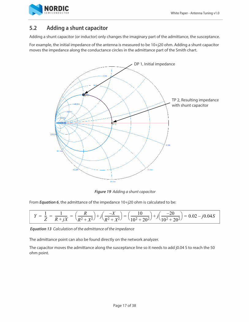
5.2 Adding a shunt capacitorAdding a shunt capacitor (or inductor) only changes the imaginary part of the admittance, the susceptance.

For example, the initial impedance of the antenna is measured to be 10+j20 ohm. Adding a shunt capacitor moves the impedance along the conductance circles in the admittance part of the Smith chart.

Figure 19 Adding a shunt capacitor

From Equation 6, the admittance of the impedance 10+j20 ohm is calculated to be:

Equation 13 Calculation of the admittance of the impedance

The admittance point can also be found directly on the network analyzer.

The capacitor moves the admittance along the susceptance line so it needs to add j0.04 S to reach the 50 ohm point.


TP 2, Resulting impedancewith shunt capacitor

Y1Z--- 1

R jX+--------------- R

R2 X2+------------------ j

X–R2 X2+------------------ 10

102 202+----------------------- j

20–102 202+----------------------- 0.02 j0.04S–=+=+= = =

Page 17 of 38


To calculate the capacitor value, use the equation from Equation 7:

Equation 14 Calculating the capacitor value

This means the shunt capacitor should be 2.65 pF to get 50 ohm impedance.

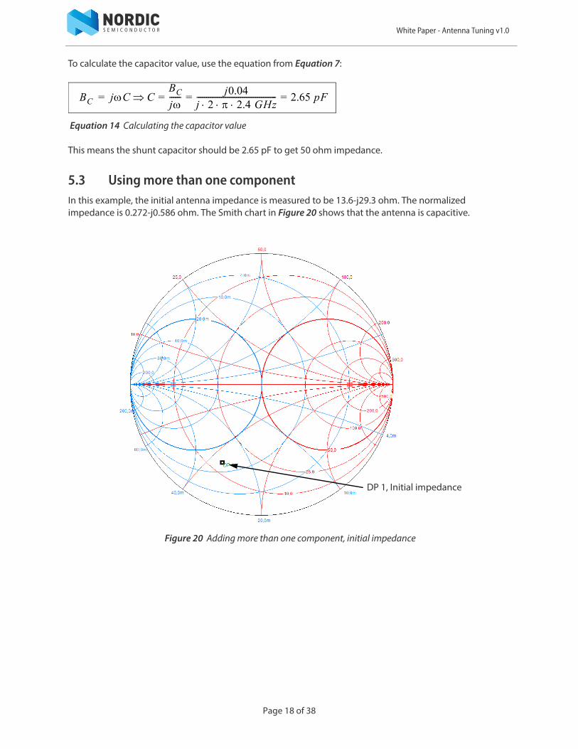
5.3 Using more than one componentIn this example, the initial antenna impedance is measured to be 13.6-j29.3 ohm. The normalized impedance is 0.272-j0.586 ohm. The Smith chart in Figure 20 shows that the antenna is capacitive.

Figure 20 Adding more than one component, initial impedance

BC jC CBCj------ j0.04

j 2 2.4 GHz ------------------------------------------ 2.65 pF= = ==


Page 18 of 38


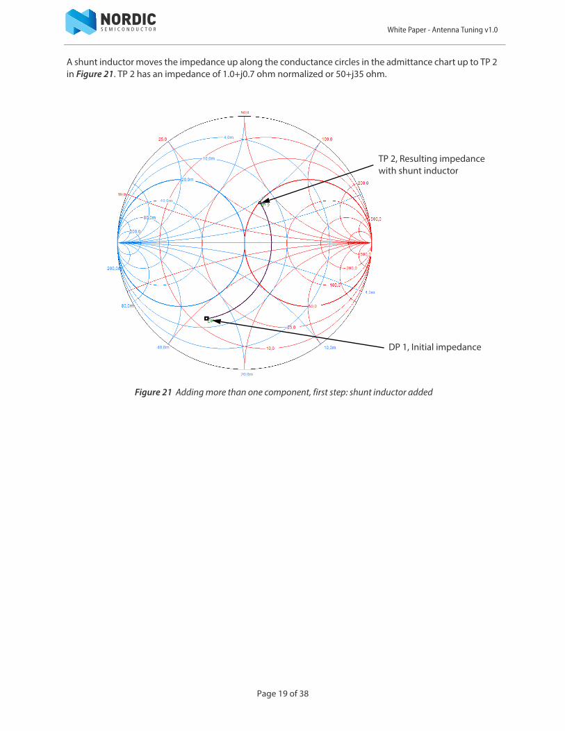
A shunt inductor moves the impedance up along the conductance circles in the admittance chart up to TP 2 in Figure 21. TP 2 has an impedance of 1.0+j0.7 ohm normalized or 50+j35 ohm.

Figure 21 Adding more than one component, first step: shunt inductor added


TP 2, Resulting impedancewith shunt inductor

Page 19 of 38


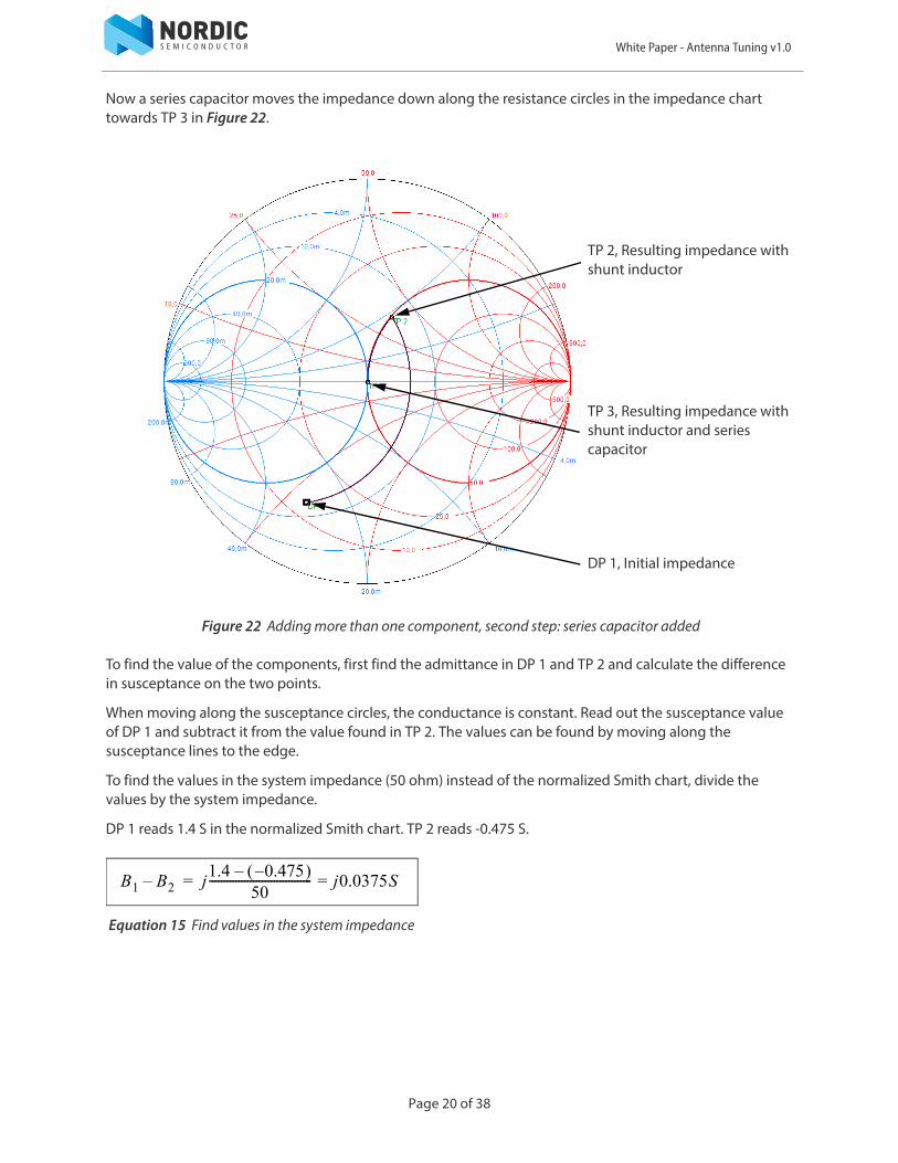
Now a series capacitor moves the impedance down along the resistance circles in the impedance chart towards TP 3 in Figure 22.

Figure 22 Adding more than one component, second step: series capacitor added

To find the value of the components, first find the admittance in DP 1 and TP 2 and calculate the difference in susceptance on the two points.

When moving along the susceptance circles, the conductance is constant. Read out the susceptance value of DP 1 and subtract it from the value found in TP 2. The values can be found by moving along the susceptance lines to the edge.

To find the values in the system impedance (50 ohm) instead of the normalized Smith chart, divide the values by the system impedance.

DP 1 reads 1.4 S in the normalized Smith chart. TP 2 reads -0.475 S.

Equation 15 Find values in the system impedance


TP 3, Resulting impedance withshunt inductor and seriescapacitor

TP 2, Resulting impedance withshunt inductor

B1 B2– j1.4 0.475– –

50----------------------------------- j0.0375S==

Page 20 of 38


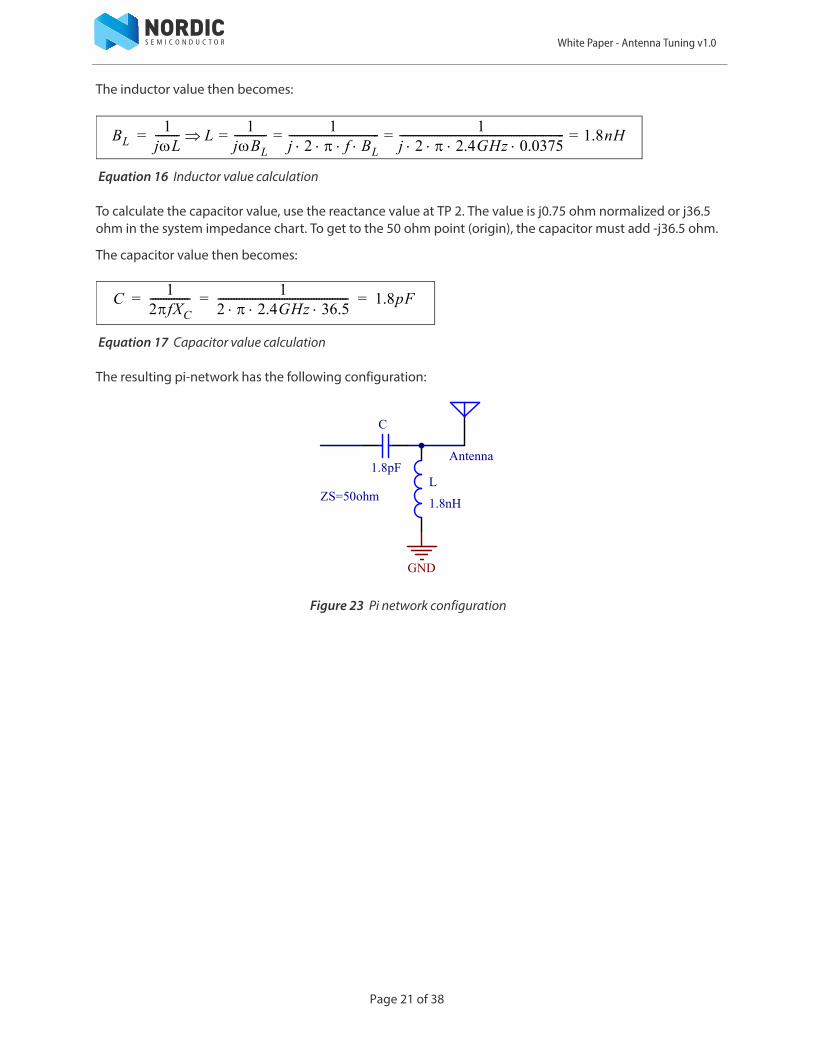
The inductor value then becomes:

Equation 16 Inductor value calculation

To calculate the capacitor value, use the reactance value at TP 2. The value is j0.75 ohm normalized or j36.5 ohm in the system impedance chart. To get to the 50 ohm point (origin), the capacitor must add -j36.5 ohm.

The capacitor value then becomes:

Equation 17 Capacitor value calculation

The resulting pi-network has the following configuration:

Figure 23 Pi network configuration

BL1jL--------- L

1jBL------------ 1

j 2 f BL ---------------------------------- 1

j 2 2.4GHz 0.0375 -------------------------------------------------------------- 1.8nH= = = ==

C1

2fXC--------------- 1

2 2.4GHz 36.5 ------------------------------------------------- 1.8pF= = =

1.8pF

C

1.8nH

LZS=50ohm

GND

Antenna

Page 21 of 38


6 Non-ideal componentsUnfortunately, there is no such thing as a perfect component. No component alters only the reactance or susceptance. All real components has parasitic effects caused by the physical housing, the terminals, and how it is mounted on the PCB.

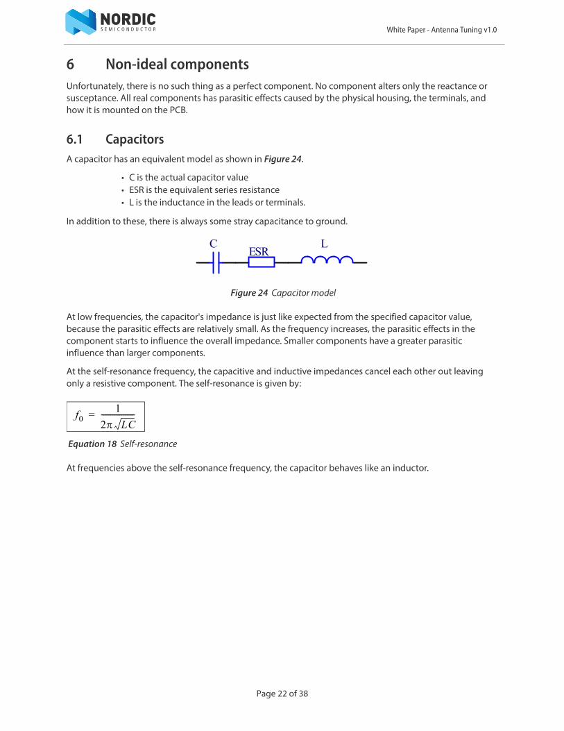
6.1 CapacitorsA capacitor has an equivalent model as shown in Figure 24.

• C is the actual capacitor value • ESR is the equivalent series resistance• L is the inductance in the leads or terminals.

In addition to these, there is always some stray capacitance to ground.

Figure 24 Capacitor model

At low frequencies, the capacitor's impedance is just like expected from the specified capacitor value, because the parasitic effects are relatively small. As the frequency increases, the parasitic effects in the component starts to influence the overall impedance. Smaller components have a greater parasitic influence than larger components.

At the self-resonance frequency, the capacitive and inductive impedances cancel each other out leaving only a resistive component. The self-resonance is given by:

Equation 18 Self-resonance

At frequencies above the self-resonance frequency, the capacitor behaves like an inductor.

CESR

L

f01

2 LC------------------=

Page 22 of 38


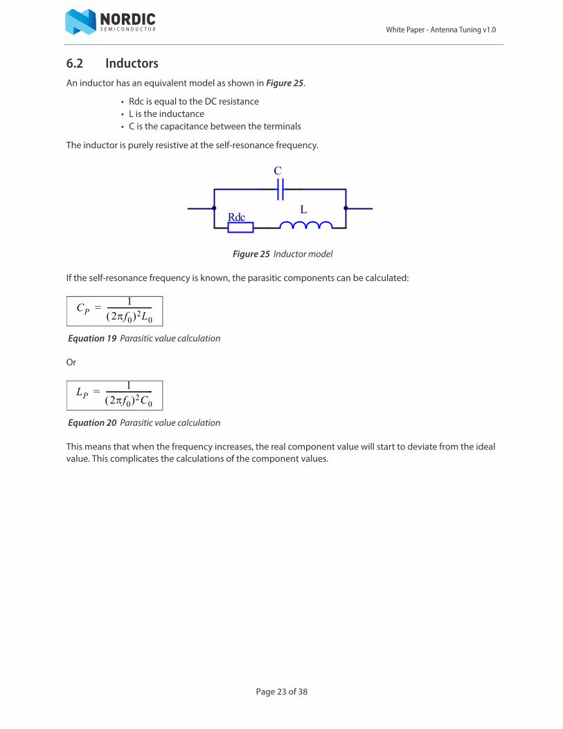
6.2 InductorsAn inductor has an equivalent model as shown in Figure 25.

• Rdc is equal to the DC resistance• L is the inductance• C is the capacitance between the terminals

The inductor is purely resistive at the self-resonance frequency.

Figure 25 Inductor model

If the self-resonance frequency is known, the parasitic components can be calculated:

Equation 19 Parasitic value calculation

Or

Equation 20 Parasitic value calculation

This means that when the frequency increases, the real component value will start to deviate from the ideal value. This complicates the calculations of the component values.

C

RdcL

CP1

2f0 2L0

------------------------=

LP1

2f0 2C0

-------------------------=

Page 23 of 38


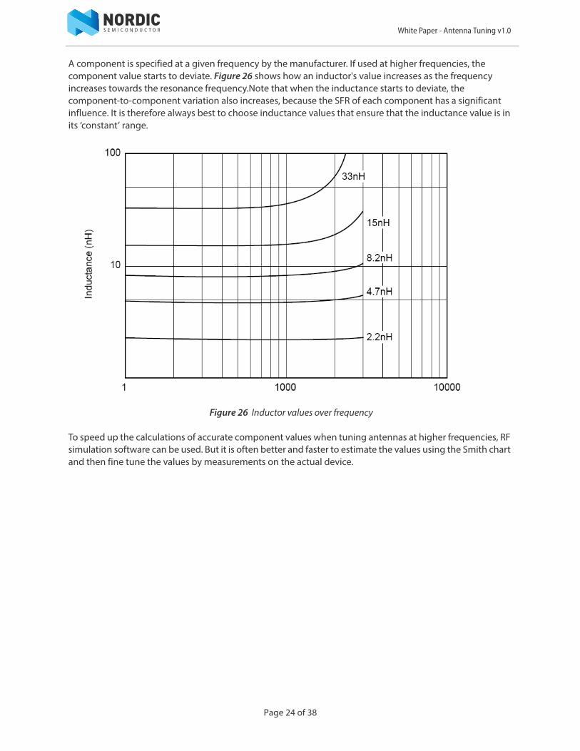
A component is specified at a given frequency by the manufacturer. If used at higher frequencies, the component value starts to deviate. Figure 26 shows how an inductor's value increases as the frequency increases towards the resonance frequency.Note that when the inductance starts to deviate, the component-to-component variation also increases, because the SFR of each component has a significant influence. It is therefore always best to choose inductance values that ensure that the inductance value is in its ‘constant’ range.

Figure 26 Inductor values over frequency

To speed up the calculations of accurate component values when tuning antennas at higher frequencies, RF simulation software can be used. But it is often better and faster to estimate the values using the Smith chart and then fine tune the values by measurements on the actual device.

Page 24 of 38


7 Equipment needed to tune an antennaFor accurate impedance measurement, a Vector Network Analyzer (VNA) must be used. The VNA measures both amplitude and phase, so it will display complex impedance values. The VNA must always be calibrated before use, to compensate for cable length and loss.

Solder a short coaxial cable to the circuit that is to be analyzed. The length of the coaxial cable can be compensated on the VNA. It is important to use short cables and solder the screen to a good ground connection close to where the impedance is to be measured. The center conductor must also be kept as short as possible to avoid adding too much series inductance.

Page 25 of 38


8 ExamplesTo better explain how the impedance matching is done, some examples are needed. Section 8.1 shows how to match a chip antenna and section 8.2 on page 33 shows how to match a ¼ wave PCB antenna.

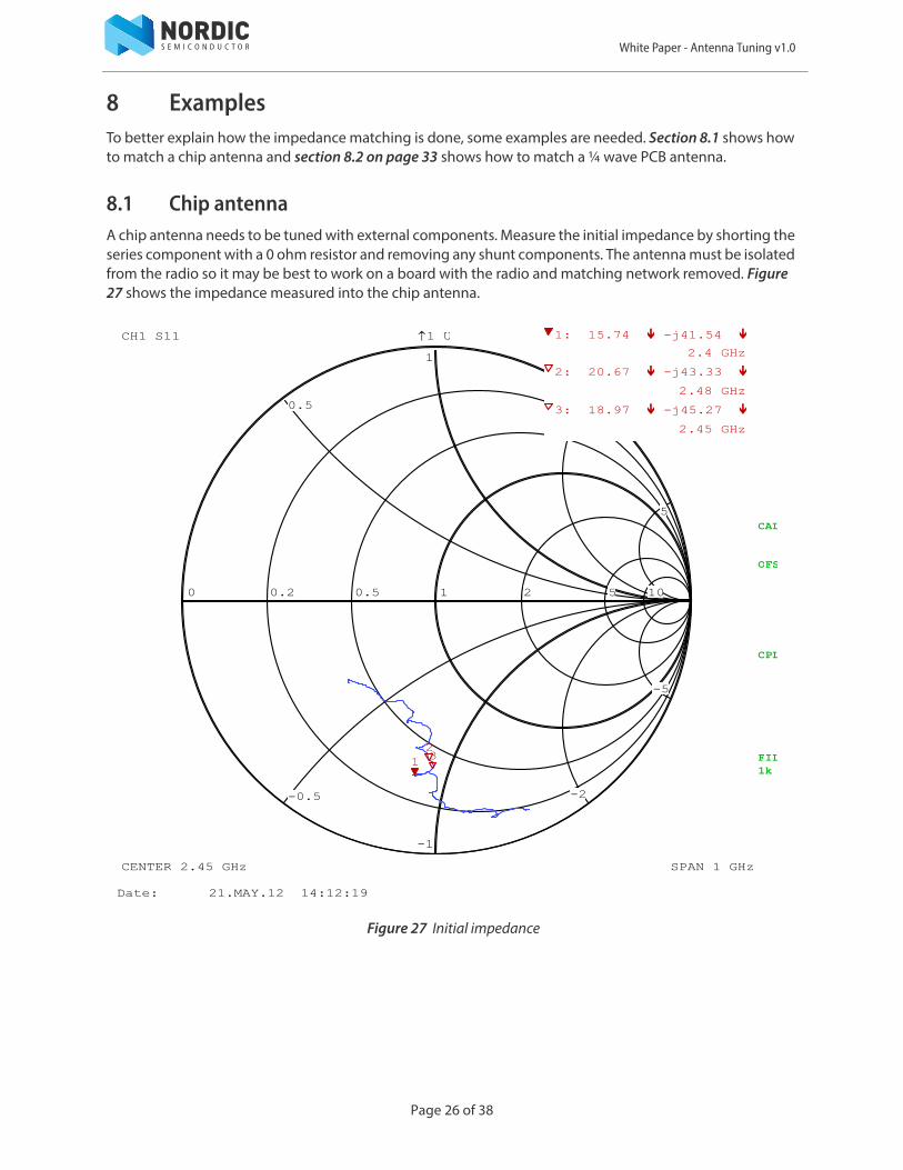
8.1 Chip antennaA chip antenna needs to be tuned with external components. Measure the initial impedance by shorting the series component with a 0 ohm resistor and removing any shunt components. The antenna must be isolated from the radio so it may be best to work on a board with the radio and matching network removed. Figure 27 shows the impedance measured into the chip antenna.


0 0.2 0.5 1 2 5 10

-5

-2

-1

-0.5

0.5

1

2

5

CH1 1 U

CENTER 2.45 GHz SPAN 1 GHz

FIL1k1kFIL1k1k

CAL

OFS

CPL

S11

123

1: 15.74 -j41.54

2.4 GHz

2: 20.67 -j43.33

2.48 GHz

3: 18.97 -j45.27

2.45 GHz

Date: 21.MAY.12 14:12:19

Page 26 of 38


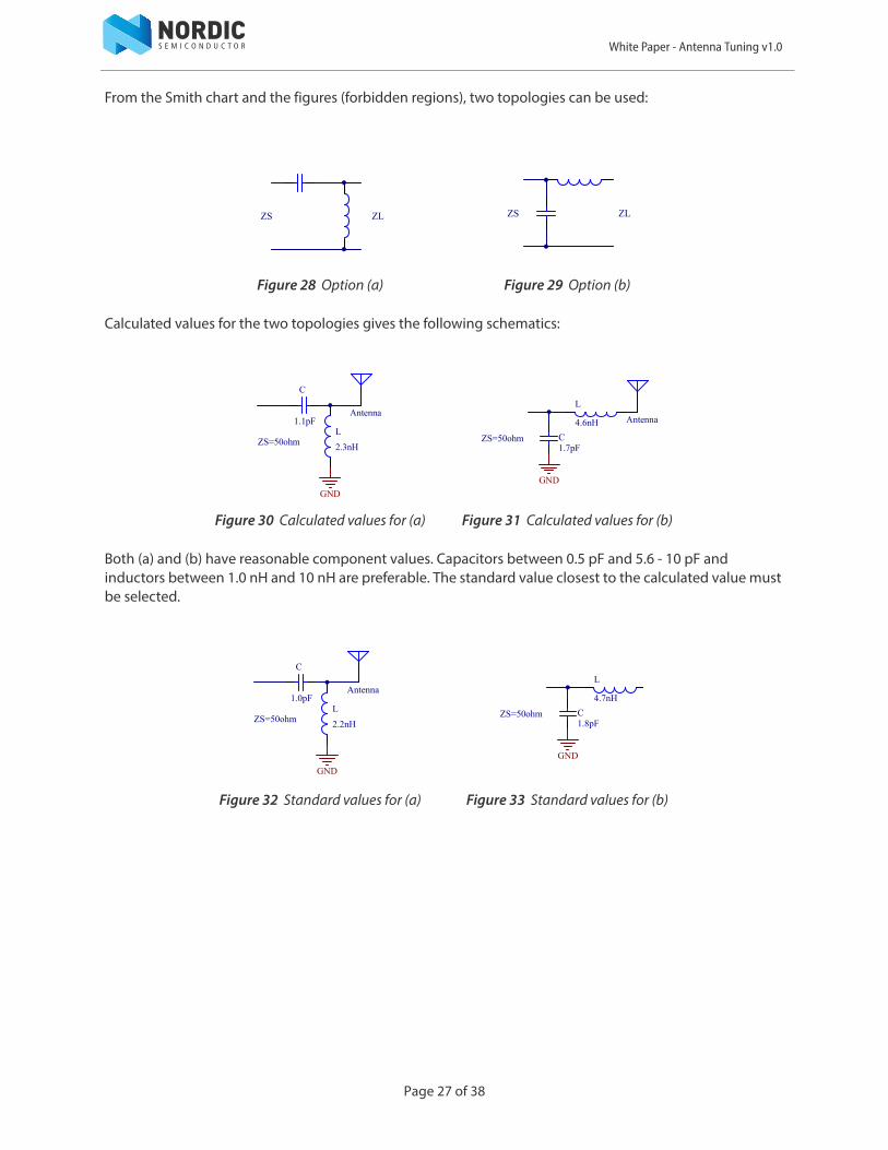
From the Smith chart and the figures (forbidden regions), two topologies can be used:

Calculated values for the two topologies gives the following schematics:

Both (a) and (b) have reasonable component values. Capacitors between 0.5 pF and 5.6 - 10 pF and inductors between 1.0 nH and 10 nH are preferable. The standard value closest to the calculated value must be selected.

Figure 28 Option (a) Figure 29 Option (b)

Figure 30 Calculated values for (a) Figure 31 Calculated values for (b)

Figure 32 Standard values for (a) Figure 33 Standard values for (b)

ZS ZL ZS ZL

1.1pF

C

2.3nH

LZS=50ohm

GND

Antenna

1.7pFC

4.6nH

L

ZS=50ohm

GND

Antenna

1.0pF

C

2.2nH

LZS=50ohm

GND

Antenna

1.8pFC

4.7nH

L

ZS=50ohm

GND

Page 27 of 38


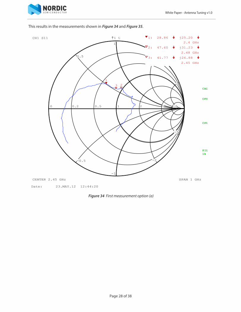
This results in the measurements shown in Figure 34 and Figure 35.

Figure 34 First measurement option (a)

0 0.2 0.5 1 2 5 10

-5

-2

-1

-0.5

0.5

1

2

5

CH1 1 U


FIL1k1kFIL1k1k

CAL

OFS

CPL

S11

1

23

1: 28.86 j25.20

2.4 GHz

2: 47.60 j31.23

2.48 GHz

3: 41.77 j26.88

2.45 GHz

Date: 23.MAY.12 12:44:20

Page 28 of 38


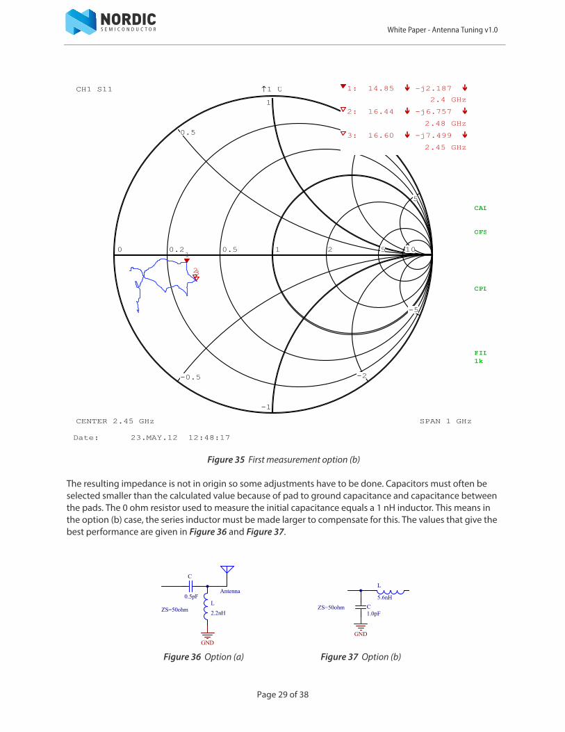
Figure 35 First measurement option (b)

The resulting impedance is not in origin so some adjustments have to be done. Capacitors must often be selected smaller than the calculated value because of pad to ground capacitance and capacitance between the pads. The 0 ohm resistor used to measure the initial capacitance equals a 1 nH inductor. This means in the option (b) case, the series inductor must be made larger to compensate for this. The values that give the best performance are given in Figure 36 and Figure 37.

Figure 36 Option (a) Figure 37 Option (b)

0 0.2 0.5 1 2 5 10

-5

-2

-1

-0.5

0.5

1

2

5

CH1 1 U


FIL1k1kFIL1k1k

CAL

OFS

CPL

S11

1

23

1: 14.85 -j2.187

2.4 GHz

2: 16.44 -j6.757

2.48 GHz

3: 16.60 -j7.499

2.45 GHz

Date: 23.MAY.12 12:48:17

0.5pF

C

2.2nH

LZS=50ohm

GND

Antenna

1.0pFC

5.6nH

L

ZS=50ohm

GND

Page 29 of 38


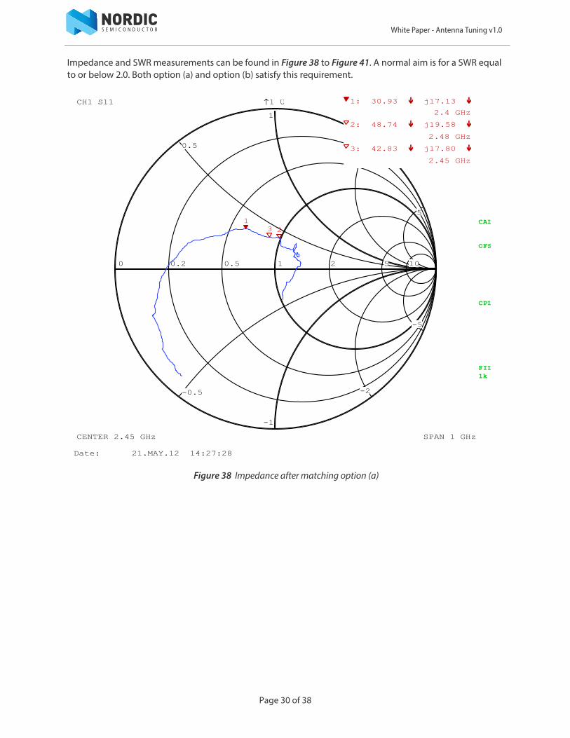
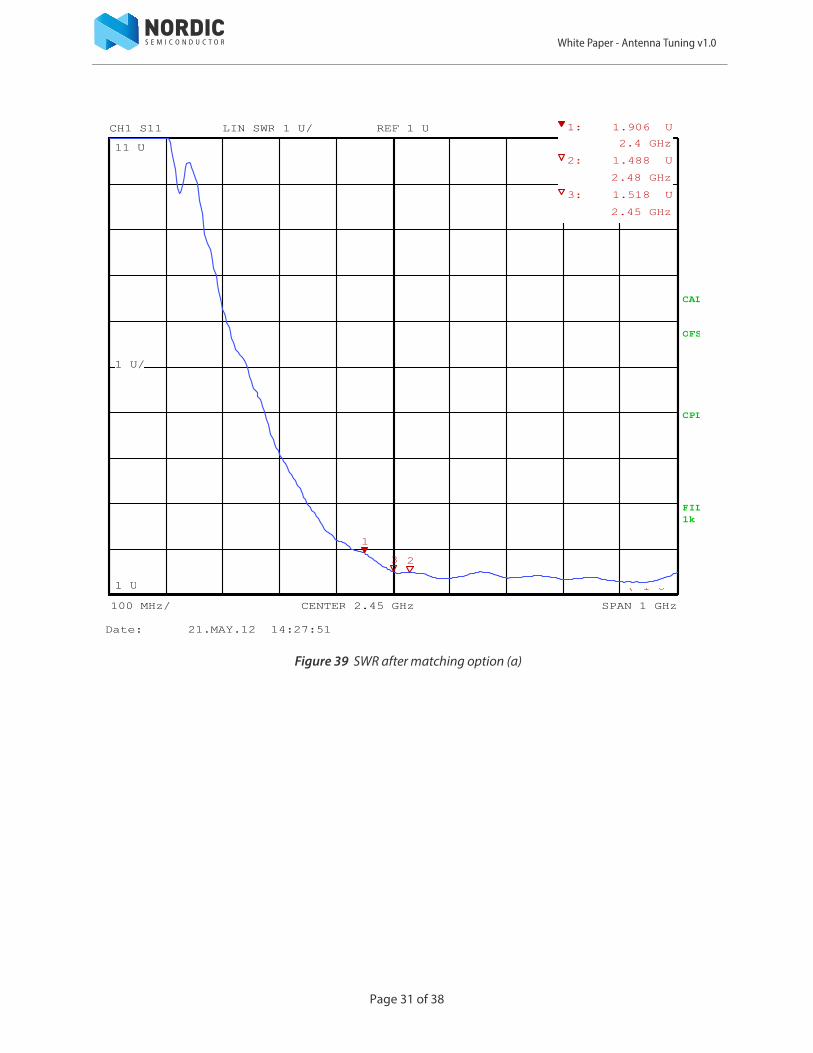
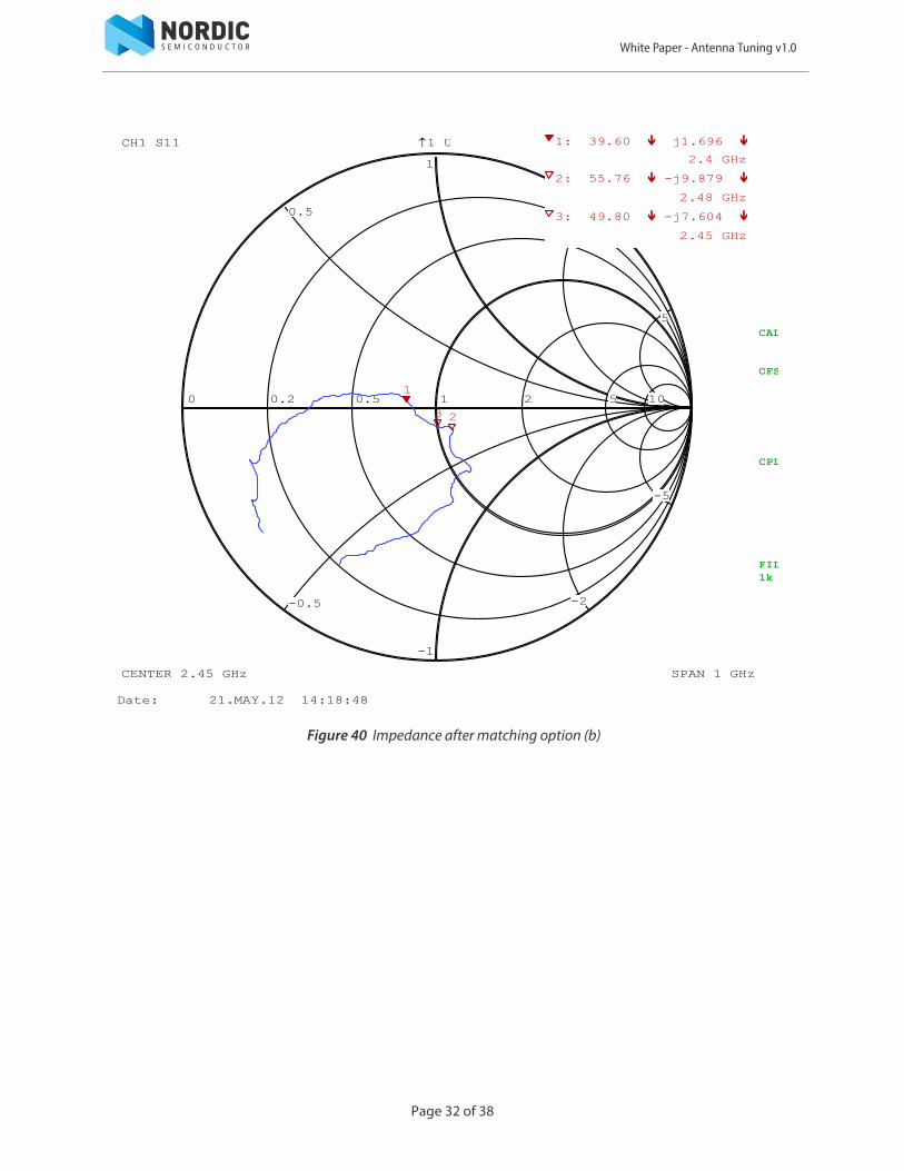
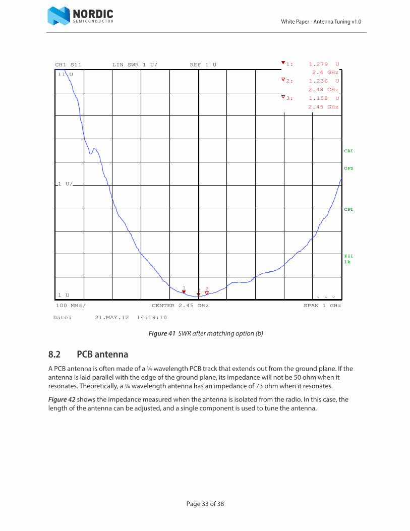
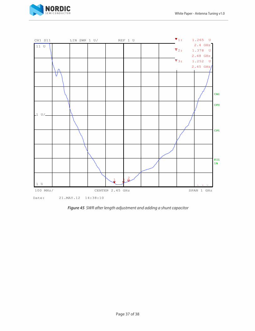
Impedance and SWR measurements can be found in Figure 38 to Figure 41. A normal aim is for a SWR equal to or below 2.0. Both option (a) and option (b) satisfy this requirement.

Figure 38 Impedance after matching option (a)

0 0.2 0.5 1 2 5 10

-5

-2

-1

-0.5

0.5

1

2

5

CH1 1 U


FIL1k1kFIL1k1k

CAL

OFS

CPL

S11

123

1: 30.93 j17.13

2.4 GHz

2: 48.74 j19.58

2.48 GHz

3: 42.83 j17.80

2.45 GHz

Date: 21.MAY.12 14:27:28

Page 30 of 38


Figure 39 SWR after matching option (a)

+400 MHz

1 U/

1 U

11 U

CH1 1 U/ REF 1 U

CENTER 2.45 GHz SPAN 1 GHz100 MHz/

SWRLIN

FIL1k1kFIL1k1k

CAL

OFS

CPL

S11

1

23

1: 1.906 U

2.4 GHz

2: 1.488 U

2.48 GHz

3: 1.518 U

2.45 GHz

1 U

Date: 21.MAY.12 14:27:51

Page 31 of 38


Figure 40 Impedance after matching option (b)

0 0.2 0.5 1 2 5 10

-5

-2

-1

-0.5

0.5

1

2

5

CH1 1 U


FIL1k1kFIL1k1k

CAL

OFS

CPL

S11

1

23

1: 39.60 j1.696

2.4 GHz

2: 55.76 -j9.879

2.48 GHz

3: 49.80 -j7.604

2.45 GHz

Date: 21.MAY.12 14:18:48

Page 32 of 38


Figure 41 SWR after matching option (b)

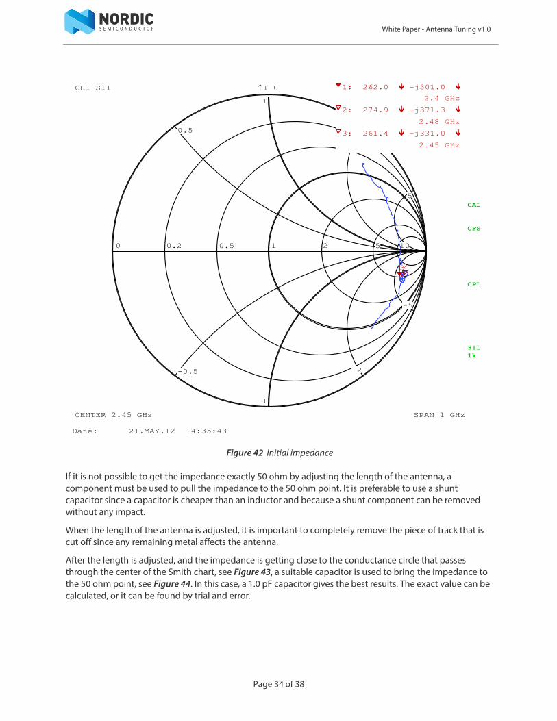
8.2 PCB antennaA PCB antenna is often made of a ¼ wavelength PCB track that extends out from the ground plane. If the antenna is laid parallel with the edge of the ground plane, its impedance will not be 50 ohm when it resonates. Theoretically, a ¼ wavelength antenna has an impedance of 73 ohm when it resonates.

Figure 42 shows the impedance measured when the antenna is isolated from the radio. In this case, the length of the antenna can be adjusted, and a single component is used to tune the antenna.

+400 MHz

1 U/

1 U

11 U

CH1 1 U/ REF 1 U


SWRLIN

FIL1k1kFIL1k1k

CAL

OFS

CPL

S11

1 23

1: 1.279 U

2.4 GHz

2: 1.236 U

2.48 GHz

3: 1.158 U

2.45 GHz

1 U

Date: 21.MAY.12 14:19:10

Page 33 of 38



If it is not possible to get the impedance exactly 50 ohm by adjusting the length of the antenna, a component must be used to pull the impedance to the 50 ohm point. It is preferable to use a shunt capacitor since a capacitor is cheaper than an inductor and because a shunt component can be removed without any impact.

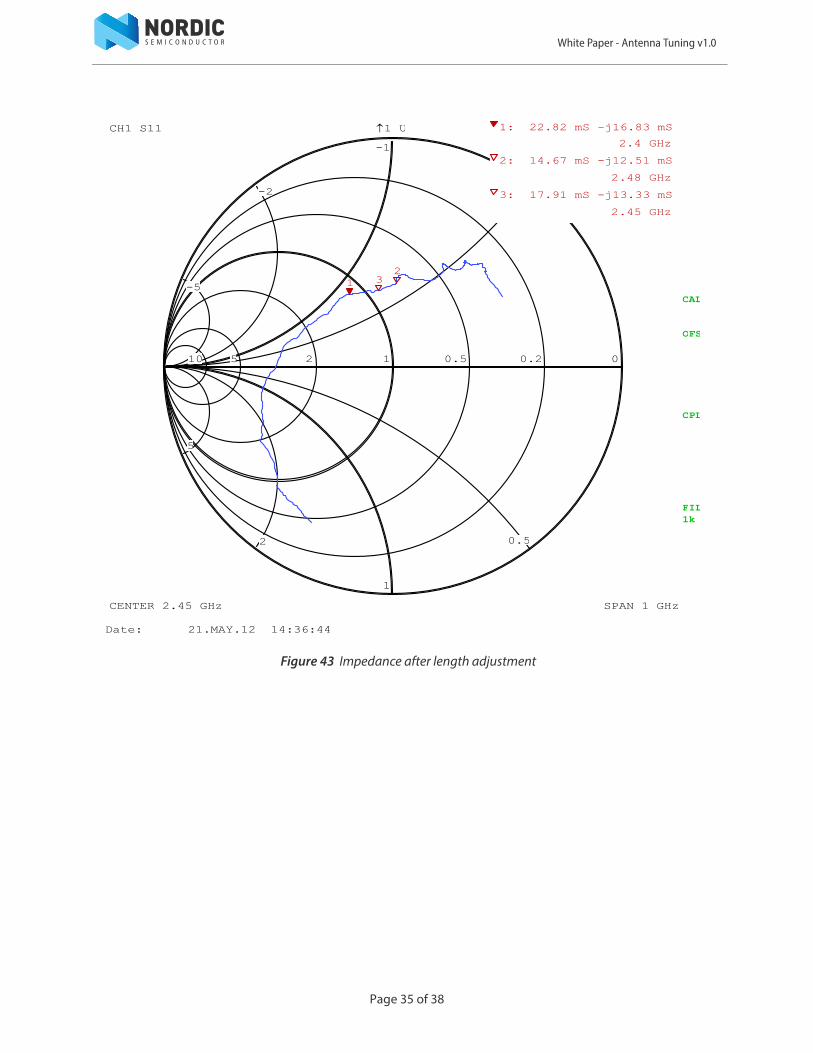
When the length of the antenna is adjusted, it is important to completely remove the piece of track that is cut off since any remaining metal affects the antenna.

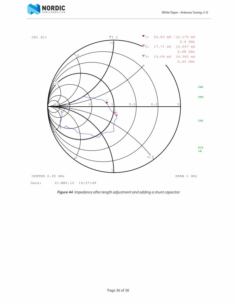
After the length is adjusted, and the impedance is getting close to the conductance circle that passes through the center of the Smith chart, see Figure 43, a suitable capacitor is used to bring the impedance to the 50 ohm point, see Figure 44. In this case, a 1.0 pF capacitor gives the best results. The exact value can be calculated, or it can be found by trial and error.

0 0.2 0.5 1 2 5 10

-5

-2

-1

-0.5

0.5

1

2

5

CH1 1 U


FIL1k1kFIL1k1k

CAL

OFS

CPL

S11

123

1: 262.0 -j301.0

2.4 GHz

2: 274.9 -j371.3

2.48 GHz

3: 261.4 -j331.0

2.45 GHz

Date: 21.MAY.12 14:35:43

Page 34 of 38


Figure 43 Impedance after length adjustment

00.20.512510

5

2

1

0.5

-0.5

-1

-2

-5

CH1 1 U


FIL1k1kFIL1k1k

CAL

OFS

CPL

S11

12

3

1: 22.82 mS -j16.83 mS

2.4 GHz

2: 14.67 mS -j12.51 mS

2.48 GHz

3: 17.91 mS -j13.33 mS

2.45 GHz

Date: 21.MAY.12 14:36:44

Page 35 of 38


Figure 44 Impedance after length adjustment and adding a shunt capacitor

00.20.512510

5

2

1

0.5

-0.5

-1

-2

-5

CH1 1 U


FIL1k1kFIL1k1k

CAL

OFS

CPL

S11

1

23

1: 24.83 mS -j2.175 mS

2.4 GHz

2: 17.71 mS j5.547 mS

2.48 GHz

3: 19.09 mS j4.362 mS

2.45 GHz

Date: 21.MAY.12 14:37:49

Page 36 of 38


Figure 45 SWR after length adjustment and adding a shunt capacitor

+400 MHz

1 U/

1 U

11 U

CH1 1 U/ REF 1 U


SWRLIN

FIL1k1kFIL1k1k

CAL

OFS

CPL

S11

1 23

1: 1.265 U

2.4 GHz

2: 1.378 U

2.48 GHz

3: 1.252 U

2.45 GHz

1 U

Date: 21.MAY.12 14:38:10

Page 37 of 38


Liability disclaimerNordic Semiconductor ASA reserves the right to make changes without further notice to the product to improve reliability, function or design. Nordic Semiconductor ASA does not assume any liability arising out of the application or use of any product or circuits described herein.

Life support applicationsNordic Semiconductor’s products are not designed for use in life support appliances, devices, or systems where malfunction of these products can reasonably be expected to result in personal injury. Nordic Semiconductor ASA customers using or selling these products for use in such applications do so at their own risk and agree to fully indemnify Nordic Semiconductor ASA for any damages resulting from such improper use or sale.

Contact detailsFor your nearest dealer, please see http://www.nordicsemi.com.Information regarding product updates, downloads, and technical support can be accessed through your My Page account on our homepage.

Revision History

Date Version Description

January 2013 1.0 First release

Main office:

Phone: +47 72 89 89 00Fax: +47 72 89 89 89

Otto Nielsens veg 127052 TrondheimNorway

Mailing address: Nordic SemiconductorP.O. Box 23367004 TrondheimNorway

Page 38 of 38

http://www.nordicsemi.no

Documents

nWP-017 Antenna tuning White paper v1.0infocenter.nordicsemi.com/pdf/nwp_017.pdf · Page 3 of 38 White Paper - Antenna Tuning v1.0 1 Antenna resonance explained The capacitance and