Nutrient export from catchments on forested landscapes

Nutrient export from catchments on forested landscapes revealscomplex nonstationary and stationary climate signals

Samson G. Mengistu,1 Christopher G. Quick,2 and Irena F. Creed1,2

Received 26 September 2012; revised 10 April 2013; accepted 8 May 2013.

[1] Headwater catchment hydrology and biogeochemistry are influenced by climate,including linear trends (nonstationary signals) and climate oscillations (stationary signals).We used an analytical framework to detect nonstationary and stationary signals in yearlytime series of nutrient export [dissolved organic carbon (DOC), dissolved organic nitrogen(DON), nitrate (NO3

�-N), and total dissolved phosphorus (TDP)] in forested headwatercatchments with differential water loading and water storage potential at the Turkey LakesWatershed in Ontario, Canada. We tested the hypotheses that (1) climate has nonstationaryand stationary effects on nutrient export, the combination of which explains most of thevariation in nutrient export ; (2) more metabolically active nutrients (e.g., DON, NO3

�-N,and TDP) are more sensitive to these signals; and (3) catchments with relatively low waterloading and water storage capacity are more sensitive to these signals. Both nonstationaryand stationary signals were identified, and the combination of both explained the majorityof the variation in nutrient export data. More variation was explained in more labilenutrients (DON, NO3

�-N, and TDP), which were also more sensitive to climate signals. Thecatchment with low-water storage potential and low water loading was most sensitive tononstationary and stationary climatic oscillations, suggesting that these hydrologic featuresare characteristic of the most effective sentinels of climate change. The observed complexlinks between climate change, climatic oscillations, and water nutrient fluxes in headwatercatchments suggest that climate may have considerable influence on the productivity andbiodiversity of surface waters, in addition to other drivers such as atmospheric pollution.

Citation: Mengistu, S. G., C. G. Quick, and I. F. Creed (2013), Nutrient export from catchments on forested landscapes revealscomplex nonstationary and stationary climate signals, Water Resour. Res., 49, doi:10.1002/wrcr.20302.

1. Introduction

[2] Scientific evidence for climate change is supportedby an increasing body of research [IntergovernmentalPanel on Climate Change (IPCC) et al., 2007; Hansen etal., 2012]. Climate directly affects water export from catch-ments by controlling water export [Mengsitu et al., 2013],and by extension may also affect the export of nutrients dis-solved in this water. However, much less is known aboutthe export of nutrients to surface waters [Whitehead et al.,2009]. Changes in nutrient export may impact water qual-ity, affecting aquatic productivity and biodiversity, andpotentially lead to algal blooms that can severely hamperhuman drinking water and recreational activities [e.g.,Paerl and Paul, 2012]. Changes in nutrient export havebeen linked to atmospheric pollution [e.g., Findlay, 2005,Watmough et al., 2005, Monteith et al., 2007], but anunderstanding of the links between climate and water

resources is needed for planning mitigation and adaptationprocedures to ensure the sustainability of water resources.

[3] Climate is inherently dynamic and contains an oftencomplex mixture of nonstationary and stationary signals.Nonstationary climate signals have means and standarddeviations that change over time, (e.g., directional climaticwarming driven by anthropogenic climate change). In con-trast, stationary climate signals have statistical means andstandard deviations that do not change over time (e.g.,global climate oscillations that are naturally occurring atscales ranging from several years to several decades). Dis-criminating nonstationary signals from the stationary sig-nals that characterize natural climatic variability willcontribute to a predictive understanding of changes in boththe quantity and quality of surface waters [Adrian et al.,2009].

[4] Lakes are a good place to detect changes in climaticconditions because they integrate all the changes that occurwithin their catchments [Williamson et al., 2008]. How-ever, headwater catchments may be the best places todetect climate signals for the following reasons: (1) theyconstitute a large spatial extent and contribute a large pro-portion of water to downstream systems [Bishop et al.,2008]; (2) they are located at relatively high-topographicpositions, they collect precipitation over a relatively smallarea, and they have thin soils for water storage, making

1Department of Earth Sciences, Western University, London, Ontario,Canada.

2Department of Biology, Western University, London, Ontario, Canada.

Corresponding author: I. F. Creed, Department of Biology, WesternUniversity, London, ON N6A 5B7, Canada. ([email protected])

©2013. American Geophysical Union. All Rights Reserved.0043-1397/13/10.1002/wrcr.20302

1

WATER RESOURCES RESEARCH, VOL. 49, 1–18, doi:10.1002/wrcr.20302, 2013

their hydrologic regime more sensitive to climate relatedchanges in environmental conditions [Strand et al., 2008];(3) their geomorphic and geologic complexity influenceshydrological flow partitioning (surface/subsurface) andpathways tapping into biogeochemical source areas [Creedet al., 1996; Creed and Band, 1998]; (4) they are found inareas that are usually relatively undisturbed by humanactivities [Blenckner et al., 2007]; and (5) there are exist-ing long term monitoring networks of headwater catch-ments particularly in the northern hemisphere [e.g., Creedet al., 2011a; Jones et al., 2012]. For these reasons, greaterfocus should be placed on headwater systems and theirpotential to serve as early warning systems for effects ofclimate change on surface water quantity and quality.

[5] In a recent study, we examined catchment wateryield responses to climate signals in a humid forest regionof eastern North America [Mengsitu et al., 2013]. Wedeveloped an approach to remove nonstationary trends andthen detect the most prominent nested oscillations withinthe data set. We found that catchments showed a generalnonstationary decline in water yields, which may havebeen caused by the 1�C per decade climate warming thathas occurred within the region over the past three decades;however, individual catchments varied in their responsive-ness to climate change. Catchments with lower water load-ing and minimal water storage capacity were most sensitiveto nonstationary signals in terms of magnitude of changeand proportion of total variation explained in yearly wateryield. These catchments were also able to explain the mostvariation in water yield through the combination of thenonstationary and stationary signals [Mengsitu et al.,2013].

[6] In this study, we extend the analysis presented inMengistu et al. [2013] to identify climate signals within nu-trient export records from the same catchments. Climatetrends and oscillations will affect nutrient export indirectlythrough alteration of water flow partitioning and pathwaysas well as directly through changes in biogeochemistry.This study tested the following hypotheses: (1) there aresignificant nonstationary and stationary signals in yearlytime series of dissolved organic carbon (DOC), dissolvedorganic nitrogen (DON), nitrate-nitrogen (NO3

�-N) andtotal dissolved phosphorus (TDP) export from headwatercatchments; (2) nonstationary trends are the major signalas a result of their greater rate of contribution to nutrientexport over time and may obscure contributions of station-ary signals on nutrient export ; (3) sensitivity to nonstation-ary signals is greater for nutrients that are moremetabolically active (e.g., DON, NO3

�-N, and TDP) thanless metabolically active (e.g., DOC) nutrients; and (4)sensitivity to these signals is greatest in catchments withrelatively low water loading and low-water storagecapacity, where the hydrological system and its hydrologi-cal connections that influence biogeochemical processesare at risk from climate change.

[7] By examining catchment nutrient export responses tochanging climatic conditions, we may be able to infer whattypes of catchments are the most sensitive sentinels of cli-mate change. These sentinel catchments could then enableus to evaluate the potential magnitude of continued climatechange effects on dissolved nutrient export to surfacewaters on forested landscapes. These sentinel catchments

could be used to support policies that seek to reduce nutri-ent loads into surface waters.

2. Study Area

[8] The Turkey Lakes Watershed (TLW) is an experi-mental forest (47�8003000N, 84�8205000W) located on theAlgoma Highlands on the northern edge of the GreatLakes-St. Lawrence Forest region and established in 1980by the Canadian federal government [Jeffries et al., 1988].

[9] The TLW rests on Precambrian silicate greenstoneformed from metamorphosed basalt, with small outcrops offelsic igneous rock near Batchawana Lake and Little Tur-key Lake [Giblin and Leahy, 1977]. The overall reliefranges from 644 m above sea level at the summit of Batch-awana Mountain to 244 m above sea level at the outlet tothe Batchawana River. A thin and discontinuous till over-lies the bedrock and ranges in depth from <1 m at higherelevations (with infrequent surface exposure of bedrock) to1–2 m at lower elevations, with till deposits up to 65 moccasionally in bedrock depressions. The podzolic soils inthe tills are thin and undifferentiated near the ridge, gradu-ally thickening, differentiating, and increasing in organiccontent on topographic benches and toward the stream,with highly humified organic deposits in wetland areas[Canada Soil Survey Committee, 1978; Creed et al., 2002].

[10] The watershed is covered by a northern hardwoodforest tolerant of shade that is dominated by sugar maple(Acer saccharum Marsh.) with no disturbances since the1950s. Average stand density (904 stems ha�1), dominantheight (20.5 m), diameter at breast height (15.3 cm) andbasal area (25.1 m2 ha�1) are relatively uniform across theuplands, with stand density increasing and dominant heightdecreasing in the wetlands. The uplands overstory includessugar maple associates, white pine (Pinus strobes L.),white spruce (Picea glauca Moench Voss.), ironwood(Ostrya virginiana (Mill.) K. Koch), and yellow birch(Betula alleghaniensis Britton), which comprise less than10% of basal area in the uplands, and the sparse understoryis dominated by saplings and seedlings of sugar maple anda variety of herbs and ferns. In the wetlands, the overstoryis a mixture of black ash (Fraxinus nigra Marsh.), easternwhite cedar (Thuja occidentalis L.), red maple (Acerrubrum L.), balsam fir (Abies balsamea (L.) Mill.), yellowbirch, and tamarack (Larix laricina (DuRoi) K. Koch.),and the understory is composed of the seedlings and sap-lings of overstory trees and various herbs and ferns [Wick-ware and Cowell, 1985; Webster et al., 2008].

[11] The watershed is influenced by a continental climate.The average annual precipitation is 1200 mm and the aver-age annual temperature is 5.0�C [based on a 28 year meteor-ological record (1981–2008) from the Canadian Air andPrecipitation Monitoring Network (CAPMoN) stationlocated just outside the TLW boundary. Meteorological con-ditions within the TLW reflect significant influences fromLake Superior in the west and orographic effects created byBatchawana Mountain. Snowpack persists from late Novem-ber, early December through to late March, early April, withpeaks in stream discharge during snowmelt and again inSeptember to November during autumn storms.

[12] The watershed is influenced by air pollution. Theaverage annual atmospheric deposition of sulfur and

MENGISTU ET AL.: NONSTATIONARY AND STATIONARY CLIMATE SIGNALS IN NUTRIENTS

2

nitrogen (based on a 26 year atmospheric acidic depositionrecord from the same CAPMoN station) show that sulfurdeposition has been declining at a rate of almost 1 kg/ha/yr,but nitrogen deposition has been comparatively stable(Figure 1; unpublished data, M. Shaw, Environment Can-ada; F. Beall, Natural Resources Canada).

[13] For this study, we examined four catchments, c35,c38, c47, and c50, that exhibit a water loading gradient inthe form of rain and snow and a water storage gradient interms of wetland area (Table 1). See Mengistu et al. [2013]for details on how the magnitudes of the gradients in waterloading and water storage were determined.

3. Methods

3.1. Analytical Framework

[14] We applied an analytical framework to identify non-stationary and stationary signals in yearly time series of nu-trient (DOC, NO3

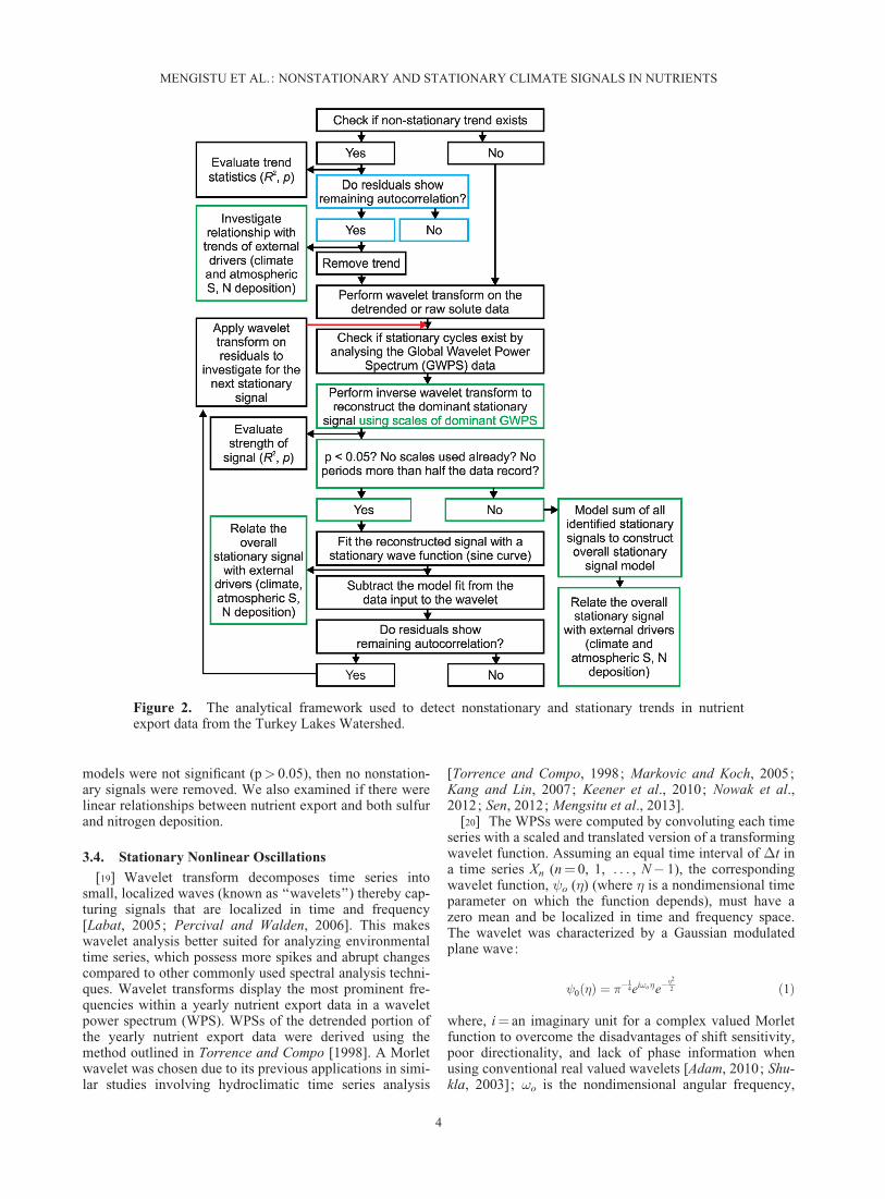
�-N, DON, and TDP) export fromcatchments c35, c38, c47, and c50 in the TLW (Figure 2)We also applied the framework to sodium export to investi-gate whether the export of this conservative nutrient mir-rored that of water yield as observed in Mengistu et al.[2013]. Daily, monthly and seasonal nutrient export datawere too variable and linear trends were not statisticallysignificant (data not shown) so yearly data were used

instead. The framework was used to capture stationaryprocesses acting on time scales greater than two yearsbecause processes with less than two years of periodicitycannot be reliably detected using yearly data. For details onthe analytical framework, please refer to Mengistu et al.[2013].

3.2. Yearly Nutrient Export

[15] Daily discharges were derived from continuouslymeasured stream stage at V-notch weirs on each catchment.The concentrations of DOC, NH4

þ-N, NO3�-N, and TDP

in discharge were derived from samples collected every 2weeks during the winter, daily during spring snowmelt, andweekly or every two weeks during the summer and autumn.Stream water samples were filtered through Fisher Q8(coarse, fast flow) paper filters. Extensive testing found nosignificant difference for samples filtered with fine versuscoarse filters (unpublished data, F. Beall, Natural Resour-ces Canada).

[16] NH4þ-N, NO3

�-N, and total dissolved nitrogen(TDN) were analyzed using sodium nitroprusside and cad-mium reduction after autoclave digestion methods, respec-tively, on Technicon Autoanalysers. DON was calculatedfrom TDN minus dissolved inorganic nitrogen(DIN¼NH4

þ-NþNO3�-N). DOC was determined by

removing dissolved inorganic carbon (DIC) by purgingwith N2 after acidification, converting DOC to DIC by per-sulfate oxidation catalyzed by UV, then converting theresulting DIC to CO2 by acidification, which was measuredby colorimetry. TDP was analyzed on a Technicon Autoan-alyzer IIC after autoclave digestion using the molybdo-phosphoric acid colour reaction. The detection limits forTDP were one ppb and most samples (more than 80%)were above this limit, particularly in catchments with largerwetlands proportions (c38 and c50).

[17] Daily nutrient concentrations were either measuredor estimated by interpolation of the two measured valueslocated directly before and directly after the unknownvalue. Daily nutrient exports were then calculated as theproduct of the total daily discharge and the interpolateddaily concentrations in the discharge. Yearly nutrientexports were calculated as the yearly sum of the daily nutri-ent exports based on the water year (1 June to 31 May),before being normalized by catchment area. Data forNO3

�-N, DON and TDP were available from 1981 to 2006and from 1988 to 2006 for DOC. A synthetic data recordfor DOC was created using regression analyses based ondischarge and the other nutrients. Coefficients of determi-nation ranged from 0.76 to 0.94.

3.3. Nonstationary Linear Trends

[18] The computed yearly time series of nutrient exportswere analyzed to determine if there were nonstationary sig-nals by linear regression. The nutrient export records forDOC, DON, NO3

�-N, and TDP passed normality (Kolmo-gorov-Smirnov), equal variance and highly influentialpoints (Cooks Distance Test and Leverage Test) tests in allfour catchments, except for DON in c50, which failed thetest of equal variance. Significant nonstationary signalswere subtracted from the observed data, and the residuals(i.e., detrended data) were then examined for the presenceof stationary signals using wavelet analysis. If regression

Figure 1. Sulfur and nitrogen atmospheric deposition inthe Turkey Lakes Watershed based on a 26 year atmos-pheric acidic deposition record.

Table 1. Physical Characteristics of the Four Catchments Fromthe Turkey Lakes Watershed Used for Analysis

c35 c38 c47 c50

Size (ha) 4.02 6.46 3.43 9.47Elevation (masl) 386 415 503 507Slope (�) 19.4 13.5 20.6 13.5Water storage (% wetland) 1.1 20.5 0.4 10.0Average precipitation (mm/yr) 1274 1257 1327 1334Average discharge (mm/yr) 632 612 555 776Average DOC export (kg/ha/yr) 13.2 12.7 47.2 32.5Average DON export (kg/ha/yr) 1.0 0.8 2.0 1.7Average NO3

�-N export (kg/ha/yr) 5.2 2.7 1.0 2.0Average TDP export (kg/ha/yr) 0.02 0.01 0.06 0.03


3

models were not significant (p> 0.05), then no nonstation-ary signals were removed. We also examined if there werelinear relationships between nutrient export and both sulfurand nitrogen deposition.

3.4. Stationary Nonlinear Oscillations

[19] Wavelet transform decomposes time series intosmall, localized waves (known as ‘‘wavelets’’) thereby cap-turing signals that are localized in time and frequency[Labat, 2005; Percival and Walden, 2006]. This makeswavelet analysis better suited for analyzing environmentaltime series, which possess more spikes and abrupt changescompared to other commonly used spectral analysis techni-ques. Wavelet transforms display the most prominent fre-quencies within a yearly nutrient export data in a waveletpower spectrum (WPS). WPSs of the detrended portion ofthe yearly nutrient export data were derived using themethod outlined in Torrence and Compo [1998]. A Morletwavelet was chosen due to its previous applications in simi-lar studies involving hydroclimatic time series analysis

[Torrence and Compo, 1998; Markovic and Koch, 2005;Kang and Lin, 2007; Keener et al., 2010; Nowak et al.,2012; Sen, 2012; Mengsitu et al., 2013].

[20] The WPSs were computed by convoluting each timeseries with a scaled and translated version of a transformingwavelet function. Assuming an equal time interval of �t ina time series Xn (n¼ 0, 1, . . . , N� 1), the correspondingwavelet function, o (�) (where � is a nondimensional timeparameter on which the function depends), must have azero mean and be localized in time and frequency space.The wavelet was characterized by a Gaussian modulatedplane wave:

0 �ð Þ ¼ ��14ei!o�e�

�2

2 ð1Þ

where, i¼ an imaginary unit for a complex valued Morletfunction to overcome the disadvantages of shift sensitivity,poor directionality, and lack of phase information whenusing conventional real valued wavelets [Adam, 2010; Shu-kla, 2003]; !o is the nondimensional angular frequency,

Figure 2. The analytical framework used to detect nonstationary and stationary trends in nutrientexport data from the Turkey Lakes Watershed.


4

which by default is taken to be 6 to satisfy the admissibilitycondition [Farge, 1992].

[21] The continuous wavelet transform of time series Xn,for each scale s at all n, with respect to the wavelet function o (�) is mathematically represented as (2):

Wn sð Þ ¼ 1

N

XN�1

n0 ¼0

xn0 ��0 � �

� ��t

s

" #ð2Þ

where, Wn (s) stands for wavelet transform coefficients, for the normalized wavelet, (�) for the complex conjugate,

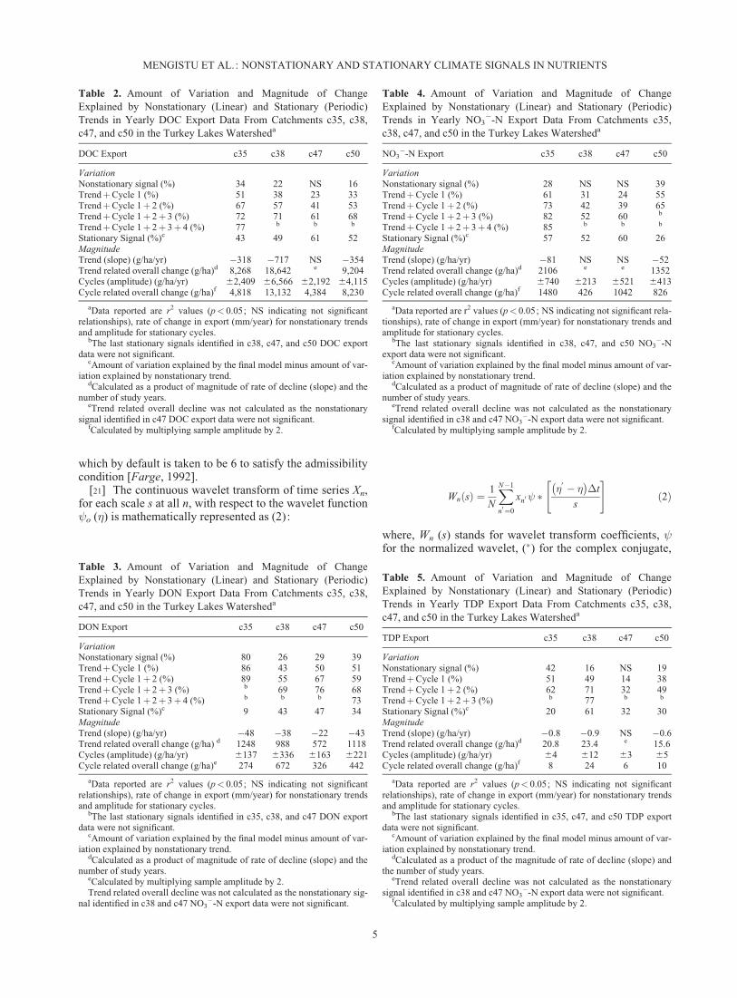
Table 2. Amount of Variation and Magnitude of ChangeExplained by Nonstationary (Linear) and Stationary (Periodic)Trends in Yearly DOC Export Data From Catchments c35, c38,c47, and c50 in the Turkey Lakes Watersheda

DOC Export c35 c38 c47 c50

VariationNonstationary signal (%) 34 22 NS 16TrendþCycle 1 (%) 51 38 23 33TrendþCycle 1þ 2 (%) 67 57 41 53TrendþCycle 1þ 2þ 3 (%) 72 71 61 68TrendþCycle 1þ 2þ 3þ 4 (%) 77 b b b

Stationary Signal (%)c 43 49 61 52MagnitudeTrend (slope) (g/ha/yr) �318 �717 NS �354Trend related overall change (g/ha)d 8,268 18,642 e 9,204Cycles (amplitude) (g/ha/yr) 62,409 66,566 62,192 64,115Cycle related overall change (g/ha)f 4,818 13,132 4,384 8,230

aData reported are r2 values (p< 0.05; NS indicating not significantrelationships), rate of change in export (mm/year) for nonstationary trendsand amplitude for stationary cycles.

bThe last stationary signals identified in c38, c47, and c50 DOC exportdata were not significant.

cAmount of variation explained by the final model minus amount of var-iation explained by nonstationary trend.

dCalculated as a product of magnitude of rate of decline (slope) and thenumber of study years.

eTrend related overall decline was not calculated as the nonstationarysignal identified in c47 DOC export data were not significant.

fCalculated by multiplying sample amplitude by 2.

Table 3. Amount of Variation and Magnitude of ChangeExplained by Nonstationary (Linear) and Stationary (Periodic)Trends in Yearly DON Export Data From Catchments c35, c38,c47, and c50 in the Turkey Lakes Watersheda

DON Export c35 c38 c47 c50

VariationNonstationary signal (%) 80 26 29 39TrendþCycle 1 (%) 86 43 50 51TrendþCycle 1þ 2 (%) 89 55 67 59TrendþCycle 1þ 2þ 3 (%) b 69 76 68TrendþCycle 1þ 2þ 3þ 4 (%) b b b 73Stationary Signal (%)c 9 43 47 34MagnitudeTrend (slope) (g/ha/yr) �48 �38 �22 �43Trend related overall change (g/ha) d 1248 988 572 1118Cycles (amplitude) (g/ha/yr) 6137 6336 6163 6221Cycle related overall change (g/ha)e 274 672 326 442


bThe last stationary signals identified in c35, c38, and c47 DON exportdata were not significant.



eCalculated by multiplying sample amplitude by 2.Trend related overall decline was not calculated as the nonstationary sig-

nal identified in c38 and c47 NO3�-N export data were not significant.

Table 4. Amount of Variation and Magnitude of ChangeExplained by Nonstationary (Linear) and Stationary (Periodic)Trends in Yearly NO3

�-N Export Data From Catchments c35,c38, c47, and c50 in the Turkey Lakes Watersheda

NO3�-N Export c35 c38 c47 c50

VariationNonstationary signal (%) 28 NS NS 39TrendþCycle 1 (%) 61 31 24 55TrendþCycle 1þ 2 (%) 73 42 39 65TrendþCycle 1þ 2þ 3 (%) 82 52 60 b

TrendþCycle 1þ 2þ 3þ 4 (%) 85 b b b

Stationary Signal (%)c 57 52 60 26MagnitudeTrend (slope) (g/ha/yr) �81 NS NS �52Trend related overall change (g/ha)d 2106 e e 1352Cycles (amplitude) (g/ha/yr) 6740 6213 6521 6413Cycle related overall change (g/ha)f 1480 426 1042 826

aData reported are r2 values (p< 0.05; NS indicating not significant rela-tionships), rate of change in export (mm/year) for nonstationary trends andamplitude for stationary cycles.

bThe last stationary signals identified in c38, c47, and c50 NO3�-N

export data were not significant.cAmount of variation explained by the final model minus amount of var-

iation explained by nonstationary trend.dCalculated as a product of magnitude of rate of decline (slope) and the

number of study years.eTrend related overall decline was not calculated as the nonstationary

signal identified in c38 and c47 NO3�-N export data were not significant.


Table 5. Amount of Variation and Magnitude of ChangeExplained by Nonstationary (Linear) and Stationary (Periodic)Trends in Yearly TDP Export Data From Catchments c35, c38,c47, and c50 in the Turkey Lakes Watersheda

TDP Export c35 c38 c47 c50

VariationNonstationary signal (%) 42 16 NS 19TrendþCycle 1 (%) 51 49 14 38TrendþCycle 1þ 2 (%) 62 71 32 49TrendþCycle 1þ 2þ 3 (%) b 77 b b

Stationary Signal (%)c 20 61 32 30MagnitudeTrend (slope) (g/ha/yr) �0.8 �0.9 NS �0.6Trend related overall change (g/ha)d 20.8 23.4 e 15.6Cycles (amplitude) (g/ha/yr) 64 612 63 65Cycle related overall change (g/ha)f 8 24 6 10


bThe last stationary signals identified in c35, c47, and c50 TDP exportdata were not significant.


dCalculated as a product of the magnitude of rate of decline (slope) andthe number of study years.

eTrend related overall decline was not calculated as the nonstationarysignal identified in c38 and c47 NO3

�-N export data were not significant.fCalculated by multiplying sample amplitude by 2.


5

s for wavelet scale, n for localized time index, and �0 fortranslated time index.

[22] The transformed signal, Wn (s), is a function of thewavelet scale, and translation parameters are found by con-ducting the convolution N (the number of data in the timeseries) times for each scale. A faster way of performingsuch a transform is to simultaneously calculate all the Nconvolutions in a Fourier space using discrete Fouriertransform of Xn (3):

x_

k ¼1

N

XN�1

n¼0

xne�2�ikn=N ð3Þ

where, k¼ 0 . . . N is the frequency index.[23] In the Fourier space the wavelet transform equation

(2) can be expressed as (4):

Wn sð Þ ¼XN�1

k¼0

x_

k _

� s!kð Þei!k n�t ð4Þ

where, _

s!ð Þ is Fourier transform of a function (t/s) and!k is an angular frequency defined as (5):

!k ¼2�k

N�tif k � N

2

� 2�k

N�tif k � N

2

8><>: ð5Þ

[24] The WPSs were calculated as the square of the abso-lute value of the wavelet transform, jWn (s)j2.

[25] Once the WPSs were calculated, the global waveletpower spectrum (GWPS) values were computed by time-averaging wavelet spectrum values over all the local spec-tra. GWPS values can be used to assess the scales (or peri-ods) contributing most to the spectral energy of the timeseries under investigation. Scales with large GWPS valueswere considered to contribute more spectral energy, whilethe contribution of small GWPS scales were assumed to belittle or insignificant. GWPS values were, therefore, used toidentify the periods of strongest stationary periodic signals.

[26] Inverse wavelet transformation of the forward wave-let transform (2) was employed to reconstruct signals basedon the coefficients of scales identified to have dominantGWPS. The inverse wavelet function is mathematicallyrepresented as (6):

xn ¼Z N

0

Z sk

s1

Wn sð Þ: �0 � �ð Þs

� �dsdn

s2ð6Þ

[27] Maintaining the coefficients of the chosen scaleswhile replacing all scale coefficients with zero and per-forming backward (inverse) wavelet transform on theresult generated the signals characterizing the identifiedscale. For choices of two or more consecutive scales,the inverse transform function builds up the recon-structed signal as the sum of wavelets of differentscales, s, at localized time, n.

[28] Autocorrelation was used to detect temporal auto-correlation within yearly nutrient export data using theautocorr function in Matlab. The confidence bounds werefound using (7):

nSTDs

6sqrt Nð Þ ð7Þ

where, nSTDs is the number of standard deviations used indetermining significance, and N is the number of independ-ent sample data points. Two standard deviations were usedto approximate 95% significance.

3.5. Detecting Stationary Signals

[29] Stationary signals were detected in the yearly nutri-ent export data using a step-wise methodology. A waveletpower spectrum of the detrended nutrient export data wasused to identify the dominant periodicity in the detrendedtime series, which was followed by an inverse wavelettransform to extract the signal of dominant periodicity cor-responding to scales of peak GWPS values. The dominantpeak was selected for further analysis only if it had notbeen selected previously, as spectral leaking from one cycleto the next could occur. The extracted signal was then fittedwith a periodic function to model and statistically analyzeif the extracted signal was stationary. The amplitude of thefitted periodic signal was not allowed to vary (i.e., had thesame amplitude throughout the 26 year data set). The samesteps were followed in the second cycle using the residualsof the detrended nutrient export data minus modeled sta-tionary signal from the first cycle as the input to the wave-let analysis). In each of the subsequent cycles, residuals(i.e., input data of the previous cycle minus modeled sta-tionary signal in the same cycle) were similarly analyzed.

[30] Subsequent peak GWPS values were considered aslong as they made a statistically significant contribution tothe regression models (p< 0.05). After selecting the sta-tionary signals for each catchment, each signal was addedto the respective nutrient export model using forward step-wise regression, starting with the nonstationary signal. Af-ter modeling the stationary structures at each step for eachnutrient, the model at each step was added to the overallnutrient model using forward step-wise regression againstthe raw nutrient export data, beginning with the nonstation-ary component of the nutrient export time series.

[31] Both individual and combined stationary signalswere assessed. For the combined stationary signals, thesum of the stationary signals identified at each step wasmodeled for each nutrient for each catchment. The ampli-tude (difference between maximum and minimum dividedby two) of the overall stationary model was used to deter-mine the range of change that was stationary over the studyperiod.

3.6. Wavelet Cross Coherence Analysis

[32] Wavelet cross-coherence analysis was used to deter-mine if there was an association between yearly indices ofglobal climate oscillations and the detrended yearly nutri-ent export data from the catchments using a Matlab pack-age based on one from Grinsted et al. [2002]. Waveletcoherence of two time series X and Y, with wavelet trans-forms Wn

X (s) and WnY (s), was defined as (8):

R2n Sð Þ ¼

jS s�1W XYn Sð Þ

� �j2

S s�1jW Xn sð Þj2

� �� S s�1jW Y

n sð Þj2� � ð8Þ


6

where, S is a smoothing operator that uses a weighted run-ning average to help locate local maxima in time and scaledirections. In the plot, this can be written as (9):

S Wð Þ ¼ Sscale Stime Wnð Þ sð Þð Þ ð9Þ

where, Sscale denotes smoothing along the wavelet scaleaxis and Stime smoothing in time axis.

[33] The Multivariate El Ni~no Southern Oscillation(ENSO) Index (MEI), Atlantic Multidecadal Oscillation(AMO), Northern Atlantic Oscillation (NAO), and PacificDecadal Oscillation (PDO) indices were selected due totheir global influence. MEI (annualized from monthly databased on water year) was used instead of alternative indices

[e.g., the Southern Oscillation index (Sea Level Pressuredifferences) and ENSO 3.4 (SST)] because it includes sixvariables: sea level pressure, surface zonal wind, meridio-nal wind, cloudiness, sea surface temperature, and surfaceair temperature [Wolter and Timlin, 1998], which makesMEI effective at discriminating ENSO impacts on hydrol-ogy, including rainfall and runoff variability [Kiem andFranks, 2001]. The annual average oscillation indices werecalculated from monthly index values. We also performedwavelet coherence analysis using the detrended sulfur andnitrogen deposition and nutrient export time series in orderto evaluate if the temporal patterns in sulfur and/or nitrogendeposition could explain the observed temporal variabilityin nutrient export from the four studied catchments.

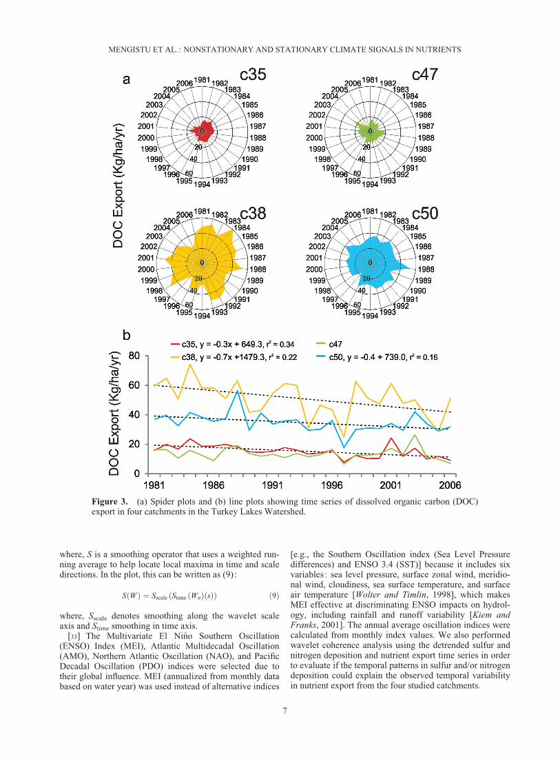
Figure 3. (a) Spider plots and (b) line plots showing time series of dissolved organic carbon (DOC)export in four catchments in the Turkey Lakes Watershed.


7

[34] Wavelet transform plots mapped the correlationsbetween wavelets of varying periods with the yearly nutri-ent flux time series to readily visualize the dominant fre-quencies, while wavelet cross coherence plots mapped thecorrelations of two wavelet-transformed time series (in thiscase time series of yearly water yield and average annualoscillation indices) at local time and space scales [Grinstedet al., 2004].

[35] Finally, Pearson Product Moment correlation testswere performed between each of the four climate indi-ces studied and sulfur and nitrogen deposition witheach of the stationary signal models isolated fromwithin the time series of each nutrient. All statisticalanalyses were completed using Sigmaplot 12.0 andMatLab version 2010b.

4. Results

4.1. Nonstationary and Stationary Signals

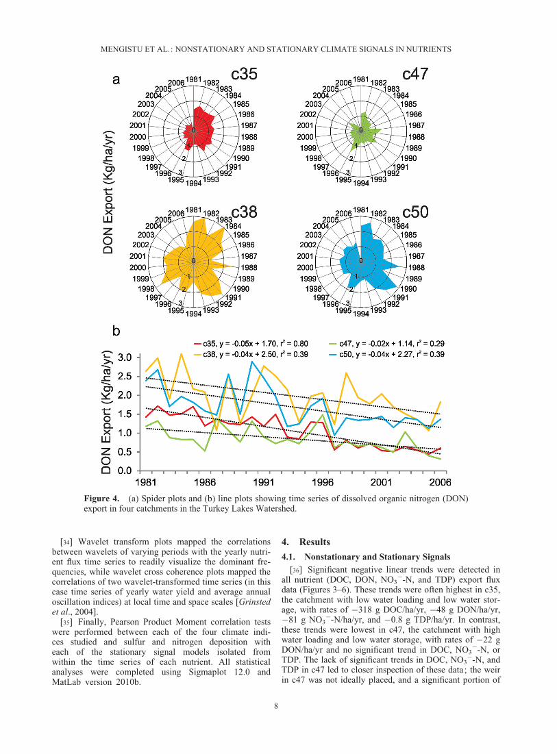
[36] Significant negative linear trends were detected inall nutrient (DOC, DON, NO3

�-N, and TDP) export fluxdata (Figures 3–6). These trends were often highest in c35,the catchment with low water loading and low water stor-age, with rates of �318 g DOC/ha/yr, �48 g DON/ha/yr,�81 g NO3

�-N/ha/yr, and �0.8 g TDP/ha/yr. In contrast,these trends were lowest in c47, the catchment with highwater loading and low water storage, with rates of �22 gDON/ha/yr and no significant trend in DOC, NO3

�-N, orTDP. The lack of significant trends in DOC, NO3

�-N, andTDP in c47 led to closer inspection of these data; the weirin c47 was not ideally placed, and a significant portion of

Figure 4. (a) Spider plots and (b) line plots showing time series of dissolved organic nitrogen (DON)export in four catchments in the Turkey Lakes Watershed.


8

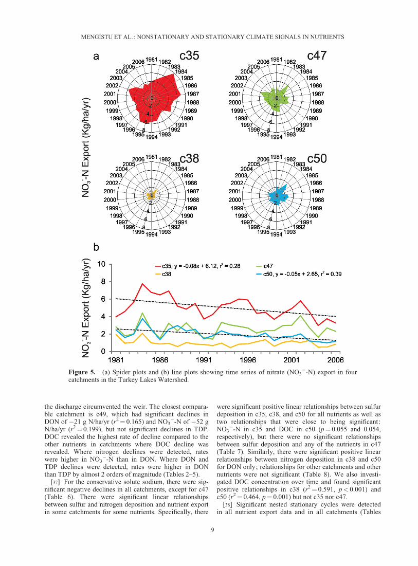
the discharge circumvented the weir. The closest compara-ble catchment is c49, which had significant declines inDON of �21 g N/ha/yr (r2¼ 0.165) and NO3

�-N of �52 gN/ha/yr (r2¼ 0.199), but not significant declines in TDP.DOC revealed the highest rate of decline compared to theother nutrients in catchments where DOC decline wasrevealed. Where nitrogen declines were detected, rateswere higher in NO3

�-N than in DON. Where DON andTDP declines were detected, rates were higher in DONthan TDP by almost 2 orders of magnitude (Tables 2–5).

[37] For the conservative solute sodium, there were sig-nificant negative declines in all catchments, except for c47(Table 6). There were significant linear relationshipsbetween sulfur and nitrogen deposition and nutrient exportin some catchments for some nutrients. Specifically, there

were significant positive linear relationships between sulfurdeposition in c35, c38, and c50 for all nutrients as well astwo relationships that were close to being significant :NO3

�-N in c35 and DOC in c50 (p¼ 0.055 and 0.054,respectively), but there were no significant relationshipsbetween sulfur deposition and any of the nutrients in c47(Table 7). Similarly, there were significant positive linearrelationships between nitrogen deposition in c38 and c50for DON only; relationships for other catchments and othernutrients were not significant (Table 8). We also investi-gated DOC concentration over time and found significantpositive relationships in c38 (r2¼ 0.591, p< 0.001) andc50 (r2¼ 0.464, p¼ 0.001) but not c35 nor c47.

[38] Significant nested stationary cycles were detectedin all nutrient export data and in all catchments (Tables

Figure 5. (a) Spider plots and (b) line plots showing time series of nitrate (NO3�-N) export in four

catchments in the Turkey Lakes Watershed.


9

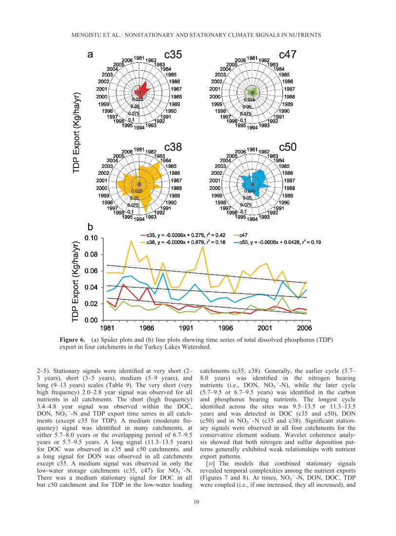
2–5). Stationary signals were identified at very short (2–3 years), short (3–5 years), medium (5–9 years), andlong (9–13 years) scales (Table 9). The very short (veryhigh frequency) 2.0–2.8 year signal was observed for allnutrients in all catchments. The short (high frequency)3.4–4.8 year signal was observed within the DOC,DON, NO3

�-N and TDP export time series in all catch-ments (except c35 for TDP). A medium (moderate fre-quency) signal was identified in many catchments, ateither 5.7–8.0 years or the overlapping period of 6.7–9.5years or 5.7–9.5 years. A long signal (11.3–13.5 years)for DOC was observed in c35 and c50 catchments, anda long signal for DON was observed in all catchmentsexcept c35. A medium signal was observed in only thelow-water storage catchments (c35, c47) for NO3

�-N.There was a medium stationary signal for DOC in allbut c50 catchment and for TDP in the low-water loading

catchments (c35, c38). Generally, the earlier cycle (5.7–8.0 years) was identified in the nitrogen bearingnutrients (i.e., DON, NO3

�-N), while the later cycle(5.7–9.5 or 6.7–9.5 years) was identified in the carbonand phosphorus bearing nutrients. The longest cycleidentified across the sites was 9.5–13.5 or 11.3–13.5years and was detected in DOC (c35 and c50), DON(c50) and in NO3

�-N (c35 and c38). Significant station-ary signals were observed in all four catchments for theconservative element sodium. Wavelet coherence analy-sis showed that both nitrogen and sulfur deposition pat-terns generally exhibited weak relationships with nutrientexport patterns.

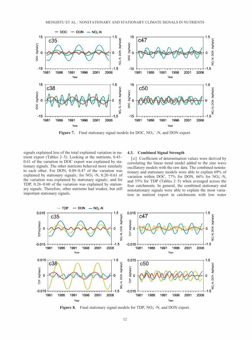
[39] The models that combined stationary signalsrevealed temporal complexities among the nutrient exports(Figures 7 and 8). At times, NO3

�-N, DON, DOC, TDPwere coupled (i.e., if one increased, they all increased), and

Figure 6. (a) Spider plots and (b) line plots showing time series of total dissolved phosphorus (TDP)export in four catchments in the Turkey Lakes Watershed.


10

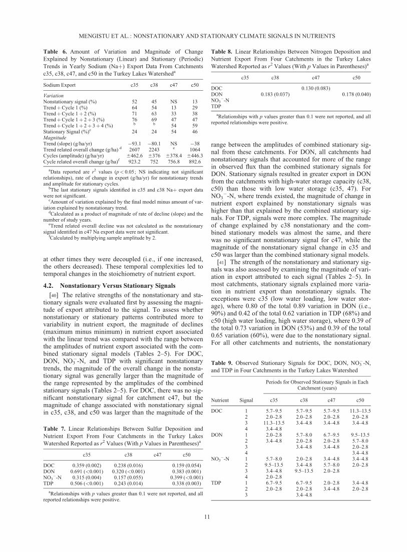
at other times they were decoupled (i.e., if one increased,the others decreased). These temporal complexities led totemporal changes in the stoichiometry of nutrient export.

4.2. Nonstationary Versus Stationary Signals

[40] The relative strengths of the nonstationary and sta-tionary signals were evaluated first by assessing the magni-tude of export attributed to the signal. To assess whethernonstationary or stationary patterns contributed more tovariability in nutrient export, the magnitude of declines(maximum minus minimum) in nutrient export associatedwith the linear trend was compared with the range betweenthe amplitudes of nutrient export associated with the com-bined stationary signal models (Tables 2–5). For DOC,DON, NO3

�-N, and TDP with significant nonstationarytrends, the magnitude of the overall change in the nonsta-tionary signal was generally larger than the magnitude ofthe range represented by the amplitudes of the combinedstationary signals (Tables 2–5). For DOC, there was no sig-nificant nonstationary signal for catchment c47, but themagnitude of change associated with nonstationary signalin c35, c38, and c50 was larger than the magnitude of the

range between the amplitudes of combined stationary sig-nal from these catchments. For DON, all catchments hadnonstationary signals that accounted for more of the rangein observed flux than the combined stationary signals forDON. Stationary signals resulted in greater export in DONfrom the catchments with high-water storage capacity (c38,c50) than those with low water storage (c35, 47). ForNO3

�-N, where trends existed, the magnitude of change innutrient export explained by nonstationary signals washigher than that explained by the combined stationary sig-nals. For TDP, signals were more complex. The magnitudeof change explained by c38 nonstationary and the com-bined stationary models was almost the same, and therewas no significant nonstationary signal for c47, while themagnitude of the nonstationary signal change in c35 andc50 was larger than the combined stationary signal models.

[41] The strength of the nonstationary and stationary sig-nals was also assessed by examining the magnitude of vari-ation in export attributed to each signal (Tables 2–5). Inmost catchments, stationary signals explained more varia-tion in nutrient export than nonstationary signals. Theexceptions were c35 (low water loading, low water stor-age), where 0.80 of the total 0.89 variation in DON (i.e.,90%) and 0.42 of the total 0.62 variation in TDP (68%) andc50 (high water loading, high water storage), where 0.39 ofthe total 0.73 variation in DON (53%) and 0.39 of the total0.65 variation (60%), were due to the nonstationary signal.For all other catchments and nutrients, the nonstationary

Table 7. Linear Relationships Between Sulfur Deposition andNutrient Export From Four Catchments in the Turkey LakesWatershed Reported as r2 Values (With p Values in Parentheses)a

c35 c38 c47 c50

DOC 0.359 (0.002) 0.238 (0.016) 0.159 (0.054)DON 0.691 (<0.001) 0.320 (<0.001) 0.383 (0.001)NO3

�-N 0.315 (0.004) 0.157 (0.055) 0.399 (<0.001)TDP 0.506 (<0.001) 0.243 (0.014) 0.338 (0.003)

aRelationships with p values greater than 0.1 were not reported, and allreported relationships were positive.

Table 6. Amount of Variation and Magnitude of ChangeExplained by Nonstationary (Linear) and Stationary (Periodic)Trends in Yearly Sodium (Naþ) Export Data From Catchmentsc35, c38, c47, and c50 in the Turkey Lakes Watersheda

Sodium Export c35 c38 c47 c50

VariationNonstationary signal (%) 52 45 NS 13TrendþCycle 1 (%) 64 54 13 29TrendþCycle 1þ 2 (%) 71 63 33 38TrendþCycle 1þ 2þ 3 (%) 76 69 47 47TrendþCycle 1þ 2þ 3þ 4 (%) b b 54 59Stationary Signal (%)c 24 24 54 46MagnitudeTrend (slope) (g/ha/yr) �93.1 �80.1 NS �38Trend related overall change (g/ha) d 2607 2243 e 1064Cycles (amplitude) (g/ha/yr) 6462.6 6376 6378.4 6446.3Cycle related overall change (g/ha)f 923.2 752 756.8 892.6

aData reported are r2 values (p< 0.05; NS indicating not significantrelationships), rate of change in export (g/ha/yr) for nonstationary trendsand amplitude for stationary cycles.

bThe last stationary signals identified in c35 and c38 Naþ export datawere not significant.



eTrend related overall decline was not calculated as the nonstationarysignal identified in c47 Na export data were not significant.


Table 8. Linear Relationships Between Nitrogen Deposition andNutrient Export From Four Catchments in the Turkey LakesWatershed Reported as r2 Values (With p Values in Parentheses)a

c35 c38 c47 c50

DOC 0.130 (0.083)DON 0.183 (0.037) 0.178 (0.040)NO3

�-NTDP

aRelationships with p values greater than 0.1 were not reported, and allreported relationships were positive.

Table 9. Observed Stationary Signals for DOC, DON, NO3�-N,

and TDP in Four Catchments in the Turkey Lakes Watershed

Nutrient Signal

Periods for Observed Stationary Signals in EachCatchment (years)

c35 c38 c47 c50

DOC 1 5.7–9.5 5.7–9.5 5.7–9.5 11.3–13.52 2.0–2.8 2.0–2.8 2.0–2.8 2.0–2.83 11.3–13.5 3.4–4.8 3.4–4.8 3.4–4.84 3.4–4.8

DON 1 2.0–2.8 5.7–8.0 6.7–9.5 9.5–13.52 3.4–4.8 2.0–2.8 2.0–2.8 5.7–8.03 3.4–4.8 3.4–4.8 2.0–2.84 3.4–4.8

NO3�-N 1 5.7–8.0 2.0–2.8 3.4–4.8 3.4–4.8

2 9.5–13.5 3.4–4.8 5.7–8.0 2.0–2.83 3.4–4.8 9.5–13.5 2.0–2.84 2.0–2.8

TDP 1 6.7–9.5 6.7–9.5 2.0–2.8 3.4–4.82 2.0–2.8 2.0–2.8 3.4–4.8 2.0–2.83 3.4–4.8


11

signals explained less of the total explained variation in nu-trient export (Tables 2–5). Looking at the nutrients, 0.43–0.61 of the variation in DOC export was explained by sta-tionary signals. The other nutrients behaved more similarlyto each other. For DON, 0.09–0.47 of the variation wasexplained by stationary signals; for NO3

�-N, 0.20–0.61 ofthe variation was explained by stationary signals; and forTDP, 0.26–0.60 of the variation was explained by station-ary signals. Therefore, other nutrients had weaker, but stillimportant stationary signals.

4.3. Combined Signal Strength

[42] Coefficient of determination values were derived bycorrelating the linear trend model added to the sine waveoscillatory models with the raw data. The combined nonsta-tionary and stationary models were able to explain 69% ofvariation within DOC, 77% for DON, 66% for NO3

�-N,and 55% for TDP (Tables 2–5) when averaged across thefour catchments. In general, the combined stationary andnonstationary signals were able to explain the most varia-tion in nutrient export in catchments with low water

Figure 7. Final stationary signal models for DOC, NO3�-N, and DON export.

Figure 8. Final stationary signal models for TDP, NO3�-N, and DON export.


12

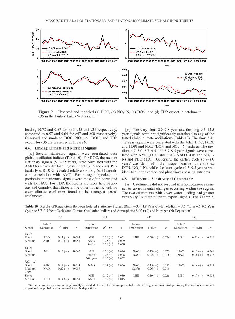
loading (0.78 and 0.67 for both c35 and c38 respectively,compared to 0.57 and 0.64 for c47 and c50 respectively).Observed and modeled DOC, NO3

�-N, DON, and TDPexport for c35 are presented in Figure 9.

4.4. Linking Climate and Nutrient Signals

[43] Several stationary signals were correlated withglobal oscillation indices (Table 10). For DOC, the medianstationary signals (5.7–9.5 years) were correlated with theAMO for low-water loading catchments (c35 and c38). Par-ticularly c38 DOC revealed relatively strong (c38) signifi-cant correlation with AMO. For nitrogen species, thepredominant stationary signals were most often correlatedwith the NAO. For TDP, the results are more heterogene-ous and complex than those in the other nutrients, with noclear climate oscillation found to be strongest acrosscatchments.

[44] The very short 2.0–2.8 year and the long 9.5–13.5year signals were not significantly correlated to any of thetested global climate oscillations (Table 10). The short 3.4–4.8 year signals were correlated with the MEI (DOC, DON,and TDP) and NAO (DON and NO3

�-N) indices. The me-dium 5.7–8.0, 6.7–9.5, and 5.7–9.5 year signals were corre-lated with AMO (DOC and TDP), NAO (DON and NO3

�-N) and PDO (TDP). Generally, the earlier cycle (5.7–8.0years) was identified in the nitrogen bearing nutrients (i.e.,DON, NO3

�-N), while the later cycle (6.7–9.5 years) wasidentified in the carbon and phosphorus bearing nutrients.

4.5. Differential Sensitivity of Catchments

[45] Catchments did not respond in a homogeneous man-ner to environmental changes occurring within the region.The two catchments with lower water loading had greatervariability in their nutrient export signals. For example,

Figure 9. Observed and modeled (a) DOC, (b) NO3�-N, (c) DON, and (d) TDP export in catchment

c35 in the Turkey Lakes Watershed.

Table 10. Results of Regressions Between Isolated Stationary Signals (Short¼ 3.4–4.8 Year Cycle; Medium¼ 5.7–8.0 or 6.7–9.5 YearCycle or 5.7–9.5 Year Cycle) and Climate Oscillation Indices and Atmospheric Sulfur (S) and Nitrogen (N) Depositiona

c35 c38 c47 c50

SignalIndex/

Deposition r2 (Dir) pIndex/



Deposition r2 (Dir) p

DOCShort PDO 0.11 (þ) 0.094 MEI 0.20 (�) 0.021 MEI 0.20 (�) 0.026 MEI 0.21 (�) 0.019Medium AMO 0.12 (�) 0.089 AMO 0.25 (�) 0.009

Sulfur 0.20 (þ) 0.029DONShort MEI 0.16 (�) 0.042 MEI 0.20 (�) 0.024 NAO 0.13 (�) 0.073 NAO 0.15 (�) 0.049Medium Sulfur 0.28 (þ) 0.008 NAO 0.22 (þ) 0.016 NAO 0.18 (þ) 0.033

Nitrogen 0.15 (þ) 0.062NO3

�-NShort Sulfur 0.12 (þ) 0.094 NAO 0.14 (þ) 0.056 NAO 0.15 (þ) 0.052 NAO 0.14 (þ) 0.057Medium NAO 0.22 (�) 0.015 Sulfur 0.26 (�) 0.010TDPShort MEI 0.12 (�) 0.089 MEI 0.19 (�) 0.025 MEI 0.17 (�) 0.038Medium PDO 0.14 (þ) 0.063 AMO 0.22 (�) 0.015

aSeveral correlations were not significantly correlated at p < 0.05, but are presented to show the general relationships among the catchments nutrientexport and the global oscillations and S and N depositions.


13

where trends exist, c35 (low water loading, low water stor-age) had the strongest linear trends [i.e., largest magnitudeof linear decline in nutrient export flux for nitrogen bearingnutrients (NO3

�-N and DON), whereas c38 (low waterloading, higher water storage) had the strongest linear trendfor DOC and TDP nutrients (Tables 2–5). Furthermore, c35generally had largest coefficient of determination values(Tables 2–5)] for nutrients that showed trends. C38 (lowwater loading, high water storage) also had stationary sig-nals with largest nutrient export amplitudes for dissolvedorganic nutrients. In contrast, the amplitude of the station-ary signal was among the weakest for c38 NO3

�-N, eventhough NO3

�-N stationary signals had a modest coefficientof determination to explain variation in c38 NO3

�-N export(Tables 2–5). C38 also had the largest coefficient of deter-mination value for TDP and generally large coefficient ofdetermination for other organic forms of nutrients (Tables2–5) A combination of catchments is needed to capture cli-mate effects on nutrient export – c35 was the most sensitiveto directional climate change, while c38 was most sensitivefor detecting climatic oscillations (Tables 2–5).

5. Discussion

[46] The effects of climate change on water quantity andquality are not clearly understood [Whitehead et al., 2009].Contributions of nonstationary and stationary climate sig-nals to nutrient export were discriminated in four catch-ments on a forested landscape. There are few studies thatfocus on the links between nutrient export from headwatercatchments and that discriminate between climate trendsversus multiple climate oscillations, so in this study wehighlight the patterns, and suggest processes to explainthem, including those that influence nutrient export throughchanges in hydrological flow partitioning and pathwaysand/or biogeochemical rates of reactions, which can betested in future studies.

5.1. Climate Signals in Nutrient Export

[47] Both nonstationary and stationary signals weredetected in nutrient export in the Turkey Lakes Watershedover a 26 year period. Nonstationary signals were declinesin nutrient export, while (multiple) stationary signals hadthe effect of increasing or decreasing the magnitude of thedecline in nutrient export. Specifically, the combination ofsignals led to larger declines in nutrient export during thewarmer/drier portions of the oscillations (reflected in posi-tive MEI, positive AMO and/or negative NAO), and tosmaller declines in export during the cooler/wetter portionsof the oscillations. There was one exception, c35, whichhad low water loading, low water storage, and wherewarmer, drier conditions lead to further increases in someof the nutrients, NO3

�-N and TDP. This finding is sup-ported by previous studies that show that during cooler,wetter water years, hydrological flow paths may beexpanded into new biogeochemical source areas (e.g., ver-tical (up the soil column) and horizontal (up the contribut-ing hillslopes into the outer extents of the variable sourcearea)) flushing nutrients from near surface and surfacesoils, while in warmer, drier water years, hydrological flowpaths may be contracted [e.g., Creed et al., 1996; Creedand Band, 1998]. The consequence is that global climate

warming appears to be leading to reduced nutrient exportthat can be further reduced when oscillations enter a warm,dry period.

[48] The multiple stationary signals occurred at veryshort (2.0–2.8 years), short (3.4–4.8 years), medium (either5.7–8.0 years or the overlapping period of 6.7–9.5 years or5.7–9.5 years), and/or occasionally at long (9.5–13.5 yearsor 11.3–13.5 years) frequencies. The very short signal wasobserved for all nutrients in all catchments but was not sig-nificantly correlated to any of the tested global climateoscillations as the periodicity of these signals were veryshort compared to the periodicity of the tested climaticoscillations. The short signal was correlated with both theMEI and NAO. This signal falls within the observed MEIperiodicity [Huggett, 1997], and the NAO does not have astatistically significant periodicity [Burroughs, 2005]. TheMEI and NAO were also significantly correlated with eachother [Mengsitu et al., 2013], which may suggest a com-mon climate oscillation influencing the catchments. Themedium signal was identified in many catchments, at either5.7–8.0 years or the overlapping period of 6.7–9.5 years or5.7–9.5 years and was most often correlated with the AMO.The periodicity of the AMO is approximately 60–90 years[Knudsen et al., 2011], but previous work has shown thatthe AMO is strongly correlated with temperature in theAlgoma Highlands and may explain about half of theobserved temperature increase in the area over the pastthree decades [Mengsitu et al., 2013]. The long signal wasnot significantly correlated to any of the four global climateoscillations. These findings suggest that multiple oscilla-tions are controlling nutrient export and that some arelinked to global climatic oscillations and others are not(and remain unexplained) in part because longer time seriesare needed.

5.2. Nonstationary Signals Obscure the Contributionsof Stationary Signals

[49] Compared to stationary signals, nonstationary sig-nals contribute more to the overall change in nutrientexport dynamics due to having higher rates of decline innutrient export resulting greater cumulative changes overtime. For catchments with observed nonstationary signals,the magnitudes of decline associated with the nonstationarysignals during the study period were compared with theranges between the amplitudes of the combined stationarysignals (Tables 2–5). Nonstationary signals obscure thecontributions of stationary signals as nonstationary signalsrevealed greater overall decline in the magnitude of nutri-ent export (approximately 8268–18,642 g/ha for DOC;572–1248 g/ha for DON; 1352–2106 g/ha for NO3

�-N;16–23 g/ha for TDP) compared to the ranges explained bythe amplitudes of the combined stationary signals (approxi-mately 4384–13,132 g/ha for DOC; 274–672 g/ha forDON: 426–1480 g/ha for NO3

�-N; 6–24 g/ha for TDP).[50] The data set available allowed us to observe station-

ary signals in nutrient export with relatively long periods(10–14 years). However, it is possible that what is beingobserved as nonstationary signals are in fact the result ofstationary signals with periods longer than could beobserved with our data set. Mengistu et al. [2013] investi-gated long-term meteorological data and found that 55% ofthe increasing temperature in the TLW over the past thirty


14

years could be ascribed to a coincident increase in valuesof the AMO index. Similar effects for nutrient export arealso possible, although they could not be detected with thelength of data set available, emphasizing the need for con-tinued support of long-term catchment monitoring stations.Additionally, while we did not analyze monthly and sea-sonal data in the present study, accounting for these sourcesof intra-annual variation would remove more noise andclarify the role of stationary signals in nutrient export.

[51] There were significant linear relationships betweensulfur deposition and nutrient export (Table 7) and few sig-nificant linear relationships between nitrogen depositionand nutrient export (Table 8), consistent with the observa-tion that both sulfur deposition (Figure 1) and nutrientexport (Figures 3–6) declined, while nitrogen deposition(Figure 1) did not change over the time series. Theobserved declines in sulfur deposition and absence ofdecline in nitrogen deposition have been observed in for-ested catchments in North America and Europe [Watmoughet al., 2005]. Also, the observed increases in DOC concen-trations that are coincident with decreases in sulfur deposi-tion have been observed in watersheds in North Americaand Europe [Monteith et al., 2007]. The lack of strong cor-relations from wavelet coherence analysis between sulfurand nitrogen deposition and nutrient export suggests thatany link between the sulfur deposition and nutrient exportis being driven by nonstationary signals (like decreases insulfur deposition) and not stationary signals (like climaticeffects), and suggests that nitrogen deposition and nutrientexport are not linked.

[52] It is also possible that some of the observed nonsta-tionary and stationary signals in nutrient export are due tononclimatic factors, including biological processes likeinsect outbreaks or pathogens. However, there is no knownoccurrence of any biological or physical phenomena in theTurkey Lakes Watershed that would have these effects. Itis also possible that more localized climate factors, like soilfrost events and or ice storm damage, are influencing nutri-ent export. We hope to be able to account for these types ofevents by investigating more fine temporal scales.

5.3. Differential Sensitivity of Metabolically LabileVersus Recalcitrant Nutrients

[53] Both nonstationary and stationary climate signalswere observed to affect nutrient export fluxes. First, fornonstationary signals, Mengistu et al. [2013] reported anaverage decline in water yields of 9.2 mm/yr among thesesame catchments, a result confirmed in the present studywith observed negative declines in the conservative solutesodium. Significant negative trends were detected in DOC,DON, NO3

�-N, and TDP export flux data. The decrease inDOC export flux was accompanied by an increase in DOCexport concentration, and other studies have reported anincrease in DOC concentrations, both in North America[Eimers et al., 2008] and Europe [Worrall and Burt, 2007;Sarkkola et al., 2009]. Dillon and Molot [2005] observed amuch greater decrease in total phosphorus and DON com-pared to DOC in Dorset, Ontario, suggesting that mobiliza-tion of these nutrients from wetlands is sensitive to changesin water table position and redox levels. It is possible thatDON, NO3

�-N, and TDP are more labile than DOC [Ste-phanauskas et al., 2000; Hendrickson et al., 2002; Kaushal

and Lewis, 2005; Lønborg and �Alvarez-Salgdo, 2012], andthat with warmer, drier conditions, these more labilenutrients are more preferentially metabolized instead ofbeing exported. If DON, NO3

�-N, and TDP are preferen-tially metabolized, then this finding suggests that there is ashift from more to less labile DOM entering the surfacewaters as a result of climate warming trends (i.e., shift to-ward higher C/N ratios).

[54] Second, the overall magnitude of declines in nutri-ent export associated with the linear trend was comparedwith the amplitude of the nutrient export associated withthe combined stationary signal model (Tables 2–5). Forcatchments with observed nonstationary signals, the magni-tudes of decline associated with the nonstationary signals(8268–18,642 g/ha for DOC; 572–1248 g/ha for DON;1352–2106 g/ha for NO3

�-N; 16–23 g/ha for TDP) werelarger than the magnitude of the range of the combined sta-tionary signal amplitude (4384–13,132 g/ha for DOC;274–672 g/ha for DON; 426–1480 g/ha for NO3

�-N; 6–24g/ha for TDP) (Tables 2–5). If nonstationary signals arelinked to global warming (even if only 50% at most, as wasthe case for water yield reported in Mengistu et al. [2012]),then this suggests that anthropogenic global warmingtrends have had a greater role in nutrient loads than naturalglobal warming oscillations at multiple time scales of yearsto decades. The catchments with high-water storage poten-tial (c38 and c50) appeared to show larger amplitudes inthe combined stationary model of DOC, DON, and TDPexports compared to catchments of lower water storagepotential. However, the combined stationary signals fromthese catchments revealed smaller amplitude for NO3

�-Nexport.

[55] In general, nitrogen and phosphorus species appearto be more responsive (more labile) than carbon to both cli-mate trends and climate oscillations. This may be due toseveral reasons: (1) there are greater concentrations ofnitrogen and phosphorus in surface and near-surface layers(shoots and roots, litter fall) than at lower depths where cli-mate reactions dominate at the land-surface interface[Devito et al., 2000; Liu et al., 2003; Marland et al., 2003;Macrae et al., 2005]; (2) there could be higher rates oftransformation at this land-surface interface due to warmertemperatures ; (3) there could be more redox switchingfrom oxidizing to reducing environments due to risingwater tables and/or expanding/contracting surface flows[Creed et al., 2011b]; and/or (4) nitrogen and phosphoruscompounds may have greater mobility along the surface/near-surface hydrologically connected flow pathways[Creed et al., 1996; Devito et al., 2000]. These changeshave implications for the stoichiometry of exportednutrients and therefore on the productivity and biodiversityof downstream waters [Justic et al., 2005; Seitzinger et al.,2005; Donner and Scavia, 2007]. Exported nutrient stoichi-ometry is also influenced by oscillation-linked catchmentresponses in nutrient export that results in temporally com-plex relationships (in phase versus out of phase) leading tovariable ratios between ecologically important nutrients.There is little knowledge about how landscape characteris-tics along the flow path from terrestrial landscapes throughaquatic systems influences nutrient stoichiometry [Vanni etal., 2011], and this study gave an insight on the effect topo-graphic features on the temporal variation of stream


15

nutrient stoichiometry. Catchments with high-water storagepotential (c38 and c50) appeared to have highly variablestoichiometry (ratios in C:N and P:N) compared to (c35and c47),. Future studies will focus not only on DOM butalso on DOM constituents to investigate if there are differ-ences among labile versus recalcitrant DOC pools. Meas-uring DOC properties (e.g., SUVA, Fluorescence Index)might reveal a biogeochemical signature that would pro-vide insight into fate of the DOC [e.g., Thurman, 1985;McKnight et al., 2003; Cory et al., 2011].

5.4. Differential Sensitivity Among the Catchments

[56] Catchments did not respond in a homogeneous man-ner to environmental changes occurring within the region.Despite a small range in annual average water loading (upto 10%), climate had a greater effect on nutrient export sig-nals in catchments with lower water loading. The catch-ment with low water loading and low-water storagecapacity, c35, had the largest declines in nutrient exportflux for nitrogen bearing nutrients and generally had themost variation explained by nonstationary signals fornutrients that showed trends (Tables 2–5). The catchmentwith low water loading and high water storage, c38, gener-ally had stationary signals with the largest nutrient exportamplitudes, although the stationary signals were among theweakest for NO3

�-N (Tables 2–5).[57] Water storage capacity has a potentially strong

effect on nutrient export by influencing water residencetime in the catchment during which biogeochemical trans-formations can occur that may alter the fate (i.e., storageversus atmospheric or aquatic) of nutrients. For example,organic matter decomposes and is metabolized quickly dur-ing the snowfree season in catchments with low-water stor-age capacity [Ponnamperuma, 1972; Sahrawat, 2004;Moore et al., 2008]. In contrast, organic matter can betrapped in catchments with high-water storage capacity anddecomposition slows down. When the water table drops,oxidation may lead to preferential removal of more labilenutrients, and when the water table rises, the remainingmore recalcitrant nutrients will become exported as storagecapacity fills and surface water discharge increases [Web-ster et al., 2008; Creed and Beall, 2009; Creed et al.,2012].

5.5. Catchments as Sentinels of Changing NutrientExports

[58] Are headwater catchments good sentinels of climatechange? To answer this question, we consider both the pre-dictability and vulnerability of nutrient export in headwatercatchments under changing environmental conditions. Forpredictability, in most cases, the nonstationary signalsexplained less variation in nutrient export than stationarysignals, suggesting that global climate warming had asmaller (lesser) influence on nutrient export than global cli-mate oscillations. However, in c35, the catchment with lowwater storage and low water loading, the nonstationary sig-nal explained more variation, suggesting that catchmentswith few or no wetlands, and which receive relatively lesswater may be most sensitive to climate change. On thishumid landscape, catchments with less water loading andstorage appeared to be more sensitive to changes in cli-matic conditions. By examining the total variation of nutri-

ent export explained by stationary and nonstationarysignals, it is possible to understand which catchments weremost sensitive to climate. Combined signals tended toexplain more of the variation in nutrient export in catch-ments with lower water loading potential, a similar patternto that observed in water yield [Mengsitu et al., 2013].Combined signals for DOC, DON, and NO3

�-N nutrientswere strongest in c35, while c38 had the highest amount ofvariance explained TDP.

[59] For vulnerability, some catchments showed substan-tial variation in nutrient export over the observed period.Catchment c35 showed the greatest range in inorganic nu-trient export, NO3

�-N, with stationary signals varying byas much as 1480 g N/ha (average annual export for thiscatchment is 3500 g N/ha/yr, Creed and Beall [2009]) andtrends showing declines of about 81 g N/ha/yr (for a totalof more than 2000 g N/ha over the observed period). Thiscatchment has little accumulation of organic matterbecause of the steep slopes, shallow soils and minimalwater storage capacity. In contrast, c38 showed the greatestrange in the export of organic nutrients, DOC, DON, andTDP. Minimum and maximum values of the stationary sig-nals ranged by as much as 13,132 g DOC/ha, 672 g DON/ha, 24 g TDP/ha, and linear trends showed declines of 717g/ha/yr for DOC, 40 g/ha/yr for DON, and 0.9 g/ha/yr forTDP.

[60] Comparing these results with observed stationaryand nonstationary signals in water yield [Mengsitu et al.,2013], the nonstationary signal explained more variation inmagnitude than the combined stationary signals in c35 fornutrients with observed significant nonstationary signals,showing that there is a link between water yield and nutri-ent export, but there were also differences. In nearly everycase, for catchments where no nonstationary trend wasdetected, the change in nutrient export related to stationarycycles was much greater than the variation explained bythe nonstationary trends. This suggests that surface waterquality is already shifting away from historical ranges con-trolled by natural fluctuations, and this could be very im-portant for ecosystems adjusted to nutrient loadings of thepast.

[61] To effectively monitor the effects of both nonsta-tionary and stationary signals of climate on headwatercatchments, a combination of catchments is needed to cap-ture climate effects on nutrient export. The catchment withlow water loading and low water storage, c35, was themost sensitive to directional climate change, while thecatchment with low water loading and high water storage,c38, was most sensitive for detecting climatic oscillations.This suggests that catchments with relatively low waterloading and low-water storage capacity are good sentinelsfor detecting the effects of anthropogenic climate changeon nutrient export. In contrast, catchments with relativelylow water loading but high water storage are good sentinelsfor detecting natural climatic oscillations and their effecton nutrient export.

6. Conclusion

[62] Climate warming and changes in atmospheric circu-lation that leads to climatic oscillations have resulted inclear reductions in water and nutrient export from the


16

Turkey Lakes Watershed over the past three decades. Com-plex links were revealed between nonstationary and station-ary changes in climatic conditions versus nutrient export tosurface waters. More variation was explained in labilenutrients (DON, NO3

�-N, and TDP), and these nutrientswere also more sensitive to climate signals. Overall, thecatchment with lower water storage potential and low-water loading potential was the most sensitive to nonsta-tionary and stationary climatic oscillations, suggesting thatit was the most effective sentinel for a dynamic climate.Although we used one of the longest data sets available inCanada, even longer sets would allow the detection of sig-nals with longer periodicities. Applying the framework toother catchments in the Turkey Lakes Watershed andaround the world will determine the broad implications ofthese results.

[63] Acknowledgments. This research was funded by a Natural Sci-ences and Engineering Research Council of Canada (NSERC) DiscoveryGrant to IFC (217053-2009 RGPIN). The Turkey Lakes Watershed isdirected by several federal government agencies, and we sincerelyacknowledge the enormous contributions by R. Semkin, D. Jeffries (Envi-ronment Canada, National Water Research Institute), and F. Beall, J. Nic-olson (Natural Resources Canada, Great Lakes Forestry Centre) to createand maintain the Turkey Lakes Watershed database, without which thisstudy would not have been possible. We thank M. Shaw for access tounpublished sulfur and nitrogen deposition data. We thank the staff at theGreat Lakes Forestry Centre Water Chemistry Laboratory for water sampleanalyses. We also thank Mr. Johnston Miller for his assistance with editingthe manuscript and preparing the graphics.

ReferencesAdam, I. (2010), Complex wavelet transform: Application to denoising, Ph.

D. thesis, Politehnica Univ. of Timisoara and Univ. de Rennes 1, Timi-soara and Rennes, Romania and France.

Adrian, R., et al. (2009), Lakes as sentinels of climate change, Limnol. Oce-anogr., 54(6), 2283–2297.

Bishop, K., I. Buffam, M. Erlandsson, J. Fölster, H. Laudon, J. Seibert, andJ. Temnerud (2008), Aqua incognita: The unknown headwaters, Hydrol.Proc., 22(8), 1239–1242, doi:10.1002/hyp.7049.

Blenckner, T., et al. (2007), Large scale climatic signatures in lakes acrossEurope: A meta analysis, Global Change Biol., 13(7), 1314–1326,doi:10.1111/j.1365-2486.2007.01364.x.

Burroughs W. J. (2005), Cycles and periodicities, in Encyclopedia of WorldClimatology, edited by J. E. Oliver, pp. 173–177, Springer, Dordrecht,Netherlands.

Canada Soil Survey Committee (1978), Canadian System of Soil Classifica-tion, Publ. 1646, 164 pp., Dep. of Agric., Ottawa.

Cory, R. M., E. W. Boyer, and D. M. McKnight (2011), Spectral methodsto advance understanding of dissolved organic carbon dynamics in for-ested catchments, in Forest Hydrology and Biogeochemistry: Synthesisof Research and Future Directions, Ecol. Stud. Ser. no. 216, edited by D.F. Levia, D. E. Carlyle-Moses, and T. Tanaka, pp. 117–135, Springer,Heidelberg, Germany.

Creed, I. F., and L. E. Band (1998), Export of nitrogen from catchmentswithin a temperate forest: Evidence for a unifying mechanism regulatedby variable source area dynamics, Water Resour. Res., 34, 3105–3120.

Creed, I. F., and F. D. Beall (2009), Distributed topographic indicators forpredicting nitrogen export from headwater catchments, Water Resour.Res., 45, W10407, doi:200910.1029/2008WR007285.

Creed, I. F., L. E. Band, N. W. Foster, I. K. Morrison, J. A. Nicolson, R. S.Semkin, and D. S. Jeffries (1996), Regulation of nitrate-N release fromtemperate forests: A test of the N flushing hypothesis, Water Resour.Res., 32, 3337–3354.

Creed, I. F., C. G. Trick, L. E. Band, and I. K. Morrison (2002), Character-izing the spatial heterogeneity of soil carbon and nitrogen pools in theTurkey Lakes Watershed: A comparison of regression techniques, WaterAir Soil Poll. Focus, 2, 81–102.

Creed, I. F., G. Z. Sass, F. D. Beall, J. M. Buttle, R. D. Moore, and M. Don-nelly (2011a), Hydrological principles for conservation of water resour-

ces within a changing forested landscape: A state of knowledge report,Sustainable For. Manage. Network, Edmonton, Alberta.

Creed, I. F., E. M. Enanga, S. G. Mengistu, F. D. Beall, and P. Hazlett(2011b), Role of redox surfaces in explaining catchment nitrogen exportacross multiple spatial and temporal scales, Abstract presented at FallMeeting, H54F-06, AGU, San Francisco, Calif., 5–9 Dec.

Creed, I. F., K. L. Webster, G. L. Braun, R. A. Bourbonniere, and F. D.Beall (2012), Topographically regulated traps of dissolved organic car-bon create hotspots of carbon dioxide efflux from forest soils, Biogeo-chemistry, 112, 149–164.

Devito, K. J., I. F. Creed, R. L. Rothwell, and E. E. Prepas (2000), Land-scape controls on phosphorus loading to boreal lakes: Implications forthe potential impacts of forest harvesting, Can. J. Fish. Aquat. Sci.,57(10), 1977–1984, doi:10.1139/cjfas-57-10-1977.

Dillon, P. J., and L. A. Molot (2005), Long term trends in catchment exportand lake retention of DOC, DON, total Fe, and total Phosphorus: TheDorset, Ontario study, 1978–1998. J. Geophy. Res., 110, G01002,doi:10.1029/2004JG000003.

Donner, S. D., and D. Scavia (2007), How climate controls the flux of nitro-gen by the Mississippi River and the development of hypoxia in the Gulfof Mexico, Limnol. Oceanogr., 52(2), 856–861.

Eimers, M. C., S. A. Watmough, and J. M. Buttle (2008), Long-term trendsin dissolved organic carbon concentration: A cautionary note, Biogeo-chemistry, 87(1), 71–81, doi:10.1007/s10533-007-9168-1.

Farge, M. (1992), Wavelet Transforms and their applications to turbulence,Annu. Rev. Fluid Mech., 24, 395–457, doi:10.1146/annurev.fluid.24.1.395.

Findlay, S. (2005), Increased carbon transport in the Hudson River: Unex-pected consequence of nitrogen deposition?, Frontiers Ecol. Environ.,3(3), 133–137, doi:10.1890/1540-9295(2005)003[0133:ICTITH]2.0.CO;2.

Giblin P. E., and E. J. Leahy (1977), Geological compilation of the Batcha-wana sheet, Districts of Algoma and Sudbury, Ontario, Prelim. Map 302,Geol. Surv. of Can., Ontario.

Grinsted, A., J. Moore, and S. Jevrejeva (2002), Cross wavelet and waveletcoherence Matlab Package. [Available at http://www.pol.ac.uk/home/research/waveletcoherence/, accessed 15 Oct 2011.].

Grinsted, A., J. C. Moore, and S. Jevrejeva (2004), Application of the crosswavelet transform and wavelet coherence to geophysical time series,Nonlinear Proc. Geophys., 11(5/6), 561–566, doi:10.5194/npg-11-561-2004.

Hansen J., M. Sato, and R. Ruedy (2012), Perception of climate change,Proc. Natl. Acad. Sci., 109(37), E2415–E2423.

Hendrickson, J., N. Trahan, E. Stecker, and Y. Ouyang (2002), TMDL andPLRG Modeling of the Lower St. Johns River: Calculation of ExternalLoads, Tech. Rep. Ser., vol. 1, St. Johns River Water Manage. District,Palatka, Fla.

Huggett, R. J. (1997), Environmental Change: The Evolving Ecosphere,Routledge, London.

Intergovernmental Panel on Climate Change, Pachauri, R. K., and A. Rei-singer (Eds.) (2007), Climate Change 2007: Synthesis Report. Contribu-tion of Working Groups I, II and III to the Fourth Assessment Report ofthe Intergovernmental Panel on Climate Change, IPCC, Geneva.

Jeffries, D., J. Kelso, and I. Morrison (1988), Physical, chemical, and bio-logical characteristics of the Turkey Lakes Watershed, Central Ontario,Canada, Can. J. Fish. Aquat. Sci., 45, 3–13.

Jones J. A., et al. (2012), Water supply sensitivity and ecosystem resilienceto land use change, climate change, and climate variability at long-termecological research sites, Bioscience, 62, 390–344.

Justic, D., N. N. Rabalais, and R. E. Turner (2005), Coupling between cli-mate variability and coastal eutrophication: Evidence and outlook for thenorthern Gulf of Mexico, J. Sea Res., 54(1), 25–35, doi:10.1016/j.seares.2005.02.008.

Kang, S., and H. Lin (2007), Wavelet analysis of hydrological and waterquality signals in an agricultural watershed, J. Hydrol., 338(1-2), 1–14,doi:10.1016/j.jhydrol.2007.01.047.

Kaushal, S. S., and W. M. Lewis (2005), Fate and transport of organic nitro-gen in minimally disturbed montane streams of Colorado, USA, Biogeo-chemistry, 74(3), 303–321, doi:10.1007/s10533-004-4723-5.

Keener, V. W., G. W. Feyereisen, U. Lall, J. W. Jones, D. D. Bosch, and R.Lowrance (2010), El-Nino/Southern Oscillation (ENSO) influences onmonthly NO3 load and concentration, stream flow and precipitation inthe Little River Watershed, Tifton, Georgia (GA), J. Hydrol., 381(3-4),352–363, doi:10.1016/j.jhydrol.2009.12.008.


17

http://www.pol.ac.uk/home/research/waveletcoherence/

http://www.pol.ac.uk/home/research/waveletcoherence/

Kiem, A. S., and S. W. Franks (2001), On the identification of ENSO-induced rainfall and runoff variability: A comparison of methods andindices, Hydrol. Sci. J., 46(5), 715–727, doi:10.1080/02626660109492866.

Knudsen, M. F., M. S. Seidenkrantz, B. H. Jacobsen, and A. Kuijpers(2011), Tracking the Atlantic Multidecadal Oscillation through the last8,000 years, Nat. Commun., 2, 178, doi:10.1038/ncomms1186.

Labat, D. (2005), Recent advances in wavelet analyses: Part I. A review ofconcepts, J. Hydrol., 314(1-4), 275–288, doi:10.1016/j.jhydrol.2005.04.003.

Liu, W., J. E. D. Fox, and Z. Xu (2003), Nutrient budget of a montane ever-green broad-leaved forest at Ailao Mountain National Nature Reserve,Yunnan, southwest China, Hydrol. Process., 17(6), 1119–1134,doi:10.1002/hyp.1184.

L�nborg, C., and X. A. �Alvarez-Salgado (2012), Recycling versus export ofbioavailable dissolved organic matter in the coastal ocean and efficiencyof the continental shelf pump, Global Biogeochem. Cycles, 26, GB3018,doi:10.1029/2012GB004353.

Macrae, M. L., T. Redding, I. F. Creed, W. Bell, and K. J. Devito (2005),Soil, surface water and groundwater phosphorus relationships in a par-tially harvested Boreal Plain aspen catchment, For. Ecol. Manage., 206,315–329, doi:10.1016/j.foreco.2004.11.010.

Markovic, D., and M. Koch (2005), Wavelet and scaling analysis ofmonthly precipitation extremes in Germany in the 20th century: Interan-nual to interdecadal oscillations and the North Atlantic Oscillation influ-ence, Water Resour. Res., 41, W09420, doi:10.1029/2004WR003843.

Marland, G., et al. (2003), The climatic impacts of land surface change andcarbon management, and the implications for climate-change mitigationpolicy, Clim. Policy, 3(2), 149–157, doi:10.1016/S1469-3062(03)00028-7.

McKnight, D. M., E. W. Hood, and L. Klapper (2003), Trace organic moi-eties of dissolved organic material in natural waters, in Aquatic Ecosys-tems: Interactivity of Dissolved Organic Matter, edited by S. E. G.Findlay and R. L. Sinsabaugh, pp. 71–96, Academic, San Diego, Calif.

Mengistu S. G., I. F. Creed, R. J. Kulperger, and C. G. Quick (2013), Rus-sian nesting dolls effect––Using wavelet analysis to reveal non-stationary and nested stationary signals in water yield from catchmentson a northern forested landscape, Hydrol. Process., 27, 669–686,doi:10.1002/hyp.9552.

Monteith, D. T., et al. (2007), Dissolved organic carbon trends resultingfrom changes in atmospheric deposition chemistry, Nature, 450(7169),537–540, doi:10.1038/nature06316.

Moore, T. R., J. A. Trofymow, M. Siltanen, and L. M. Kozak (2008), Litterdecomposition and nitrogen and phosphorus dynamics in peatlands anduplands over 12 years in central Canada, Oecologia, 157(2), 317–325,doi:10.1007/s00442-008-1076-0.

Nowak, K., M. Hoerling, B. Rajagopalan, and E. Zagona (2012), Coloradoriver basin hydroclimatic variability, J. Clim., 25(12), 4389–4403,doi:10.1175/JCLI-D-11–00406.1.

Paerl, H. W., and V. J. Paul (2012) Climate change: Links to global expan-sion of harmful cyanobacteria. Water Res., 46, 1349–1363.

Percival, D. B., and A. T. Walden (2006), Wavelet Methods for Time SeriesAnalysis, Cambridge Ser. in Stat. and Probabilistic Math., CambridgeUniv. Press, Cambridge, U. K.

Ponnamperuma, F. N. (1972), The chemistry of submerged soils, Adv.Agron., 24, 29–96.

Sahrawat, K. (2004), Organic matter accumulation in submerged soils, Adv.Agron., 81, 169–201, doi:10.1016/S0065.2113(03)81004-0.

Sarkkola, S., H. Koivusalo, A. Lauren, P. Kortelainen, T. Mattsson, M. Pal-viainen, S. Piirainen, M. Starr, and L. Finer (2009), Trends in hydrome-teorological conditions and stream water organic carbon in borealforested catchments, Sci. Total Environ., 408(1), 92–101, doi:10.1016/j.scitotenv.2009.09.008.

Seitzinger, S. P., J. A. Harrison, E. Dumont, A. H. W. Beusen, and A. F.Bouwman (2005), Sources and delivery of carbon, nitrogen, and phos-phorus to the coastal zone: An overview of Global Nutrient Export fromWatersheds (NEWS) models and their application, Global Biogeochem.Cycles, 19(4), 1–11, GB4S01, doi:10.1029/2005GB002606.

Sen, A. K. (2012), Streamflow variability in the Southern Appalachians andatmospheric teleconnections, River Res. and Appl., 28(5), 630–636,doi:10.1002/rra.1473.

Shukla, P. D. (2003), Complex wavelet transforms and their applications,M.Phil. thesis, The Univ. of Strathclyde, Glasgow, Scotland, U. K.

Stepanauskas, R., V. F. Farjalla, L. J. Tranvik, J. M. Svensson, F. A.Esteves, and W. Graneli (2000), Bioavailability and sources of DOC andDON in macrophyte stands of a tropical coastal lake, Hydrobiologia,436(1-3), 241–248, doi:10.1023/A:1026537905947.

Strand, L. T., S. Haaland, O. Kaste, and A. O. Stuanes (2008), Natural vari-ability in soil and runoff from small headwater catchments at Storgama,Norway, Ambio, 37(1), 18–28, doi:10.1579/0044-7447(2008)37[18:NVISAR]2.0.CO;2.

Thurman, E. M. (1985), Organic Geochemistry of Natural Waters, Nijoff/Junk Publ., Boston.

Torrence, C., and G. P. Compo (1998), A practical guide to wavelet analy-sis, Br. Am. Meteorol. Soc., 79(1), 61–78.

Vanni, M. J., W. H. Renwick, A. M. Bowling, M. J. Horgan, and A. D.Christian (2011), Nutrient stoichiometry of linked catchment-lake sys-tems along a gradient of land use, Freshwater Biol., 56(5), 791–811,doi:10.1111/j.1365-2427.2010.02436.x.

Watmough, S. et al. (2005), Sulphate, nitrogen and base cation budgets at21 forested catchments in Canada, the United States and Europe, Envi-ron. Monit. Assess., 109(1-3), 1–36, doi:10.1007/s10661-005-4336-z.

Webster, K. L., I. F. Creed, R. A. Bourbonniere, and F. D. Beall (2008),Controls on the heterogeneity of soil respiration in a tolerant hardwoodforest, J. Geophys. Res., 113, G03018, doi:10.1029/2008JG000706.

Whitehead P. G., R. L. Wilby, R. W. Battarbee, M. Kernan, A. J. Wade(2009), A review of the potential impacts of climate change on surfacewater quality, Hydrol. Sci. J., 54, 101–123.

Wickware, G. M., and D. W. Cowell (1985), Forest Ecosystem Classifica-tion of the Turkey Lake Watershed, Ecol. Classif. Ser. 18, Lands Dir. En-viron., Ottawa, Canada.

Williamson, C. E., W. Dodds, T. K. Kratz, and M. A. Palmer (2008), Lakesand streams as sentinels of environmental change in terrestrial andatmospheric processes, Frontiers Ecol. Environ., 6(5), 247–254,doi:10.1890/070140.

Wolter, K., and M. S. Timlin (1998), Measuring the strength of ENSOevents: How does 1997/98 rank?, Weather, 53, 315–323.

Worrall, F., and T. P. Burt (2007), Trends in DOC concentration in GreatBritain, J. Hydrol., 346(3–4), 81–92, doi:10.1016/j.jhydrol.2007.08.021.


18

Documents

Nutrient export from catchments on forested landscapes