Embed Size (px)
Citation preview

Nur Aini Masruroh
Queuing Theory
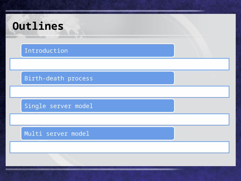
Outlines
Introduction
Birth-death process
Single server model
Multi server model
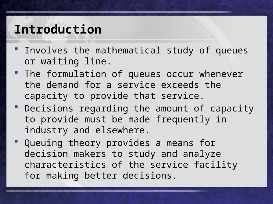
Introduction
Involves the mathematical study of queues or waiting line.
The formulation of queues occur whenever the demand for a service exceeds the capacity to provide that service.
Decisions regarding the amount of capacity to provide must be made frequently in industry and elsewhere.
Queuing theory provides a means for decision makers to study and analyze characteristics of the service facility for making better decisions.
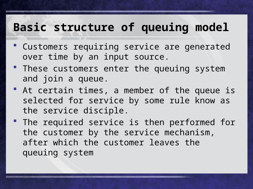
Basic structure of queuing model
Customers requiring service are generated over time by an input source.
These customers enter the queuing system and join a queue.
At certain times, a member of the queue is selected for service by some rule know as the service disciple.
The required service is then performed for the customer by the service mechanism, after which the customer leaves the queuing system
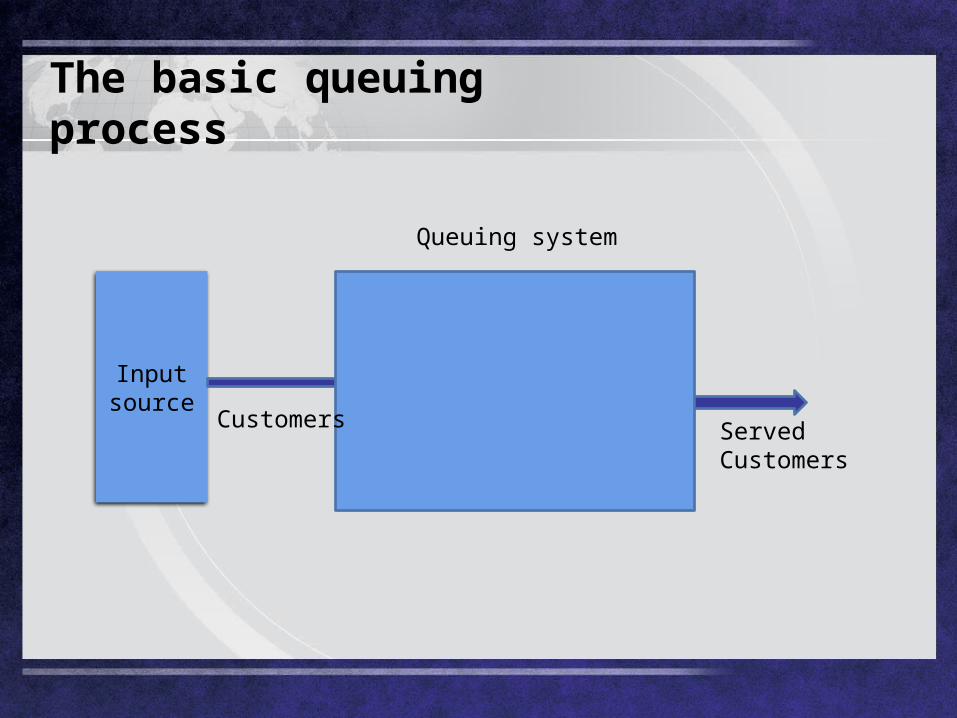
The basic queuing process
Input source Queue
Service mechanismCustomers Served
Customers
Queuing system
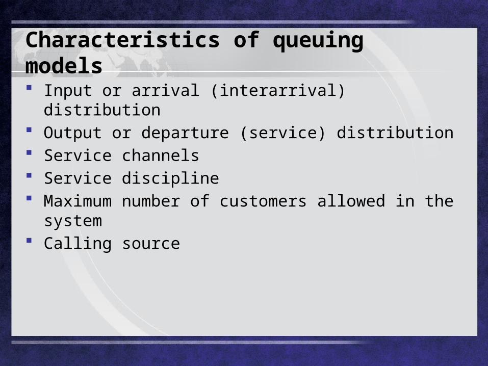
Characteristics of queuing models
Input or arrival (interarrival) distribution Output or departure (service) distribution Service channels Service discipline Maximum number of customers allowed in the system Calling source
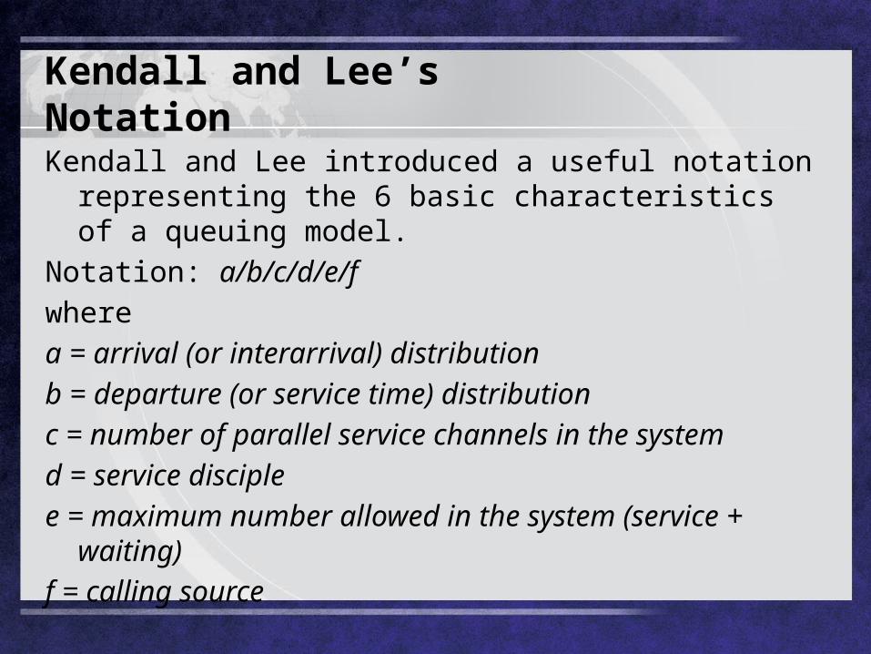
Kendall and Lee’s Notation
Kendall and Lee introduced a useful notation representing the 6 basic characteristics of a queuing model.
Notation: a/b/c/d/e/f
where
a = arrival (or interarrival) distribution
b = departure (or service time) distribution
c = number of parallel service channels in the system
d = service disciple
e = maximum number allowed in the system (service + waiting)
f = calling source
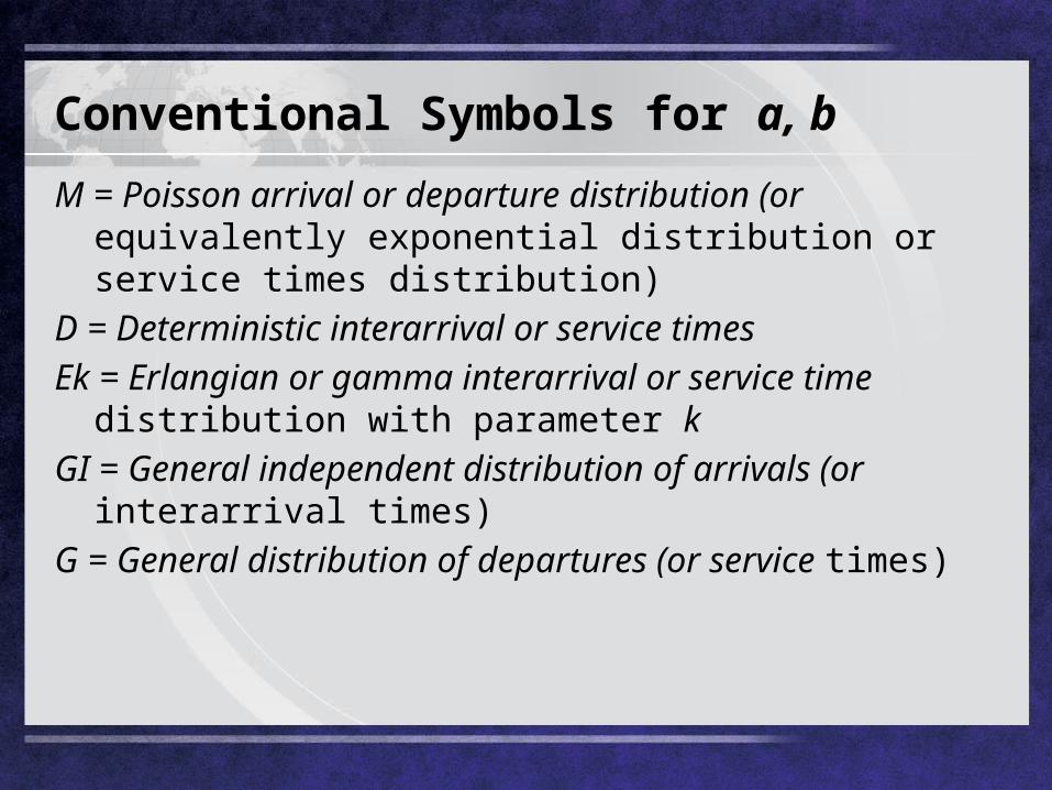
Conventional Symbols for a, b
M = Poisson arrival or departure distribution (or equivalently exponential distribution or service times distribution)
D = Deterministic interarrival or service times
Ek = Erlangian or gamma interarrival or service time distribution with parameter k
GI = General independent distribution of arrivals (or interarrival times)
G = General distribution of departures (or service times)
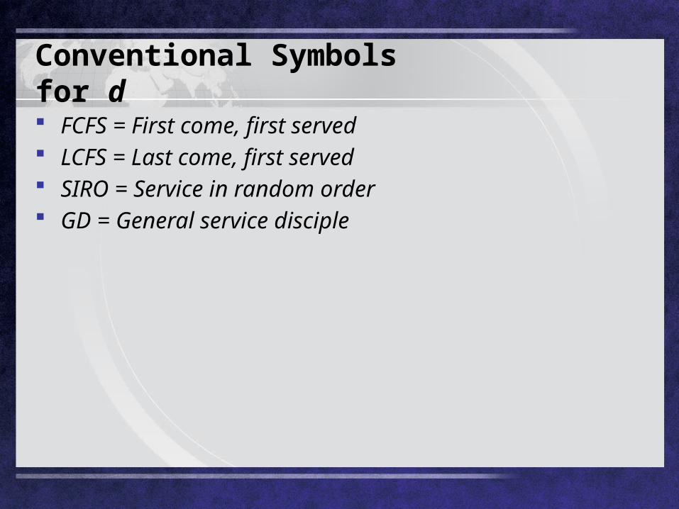
Conventional Symbols for d
FCFS = First come, first served LCFS = Last come, first served SIRO = Service in random order GD = General service disciple
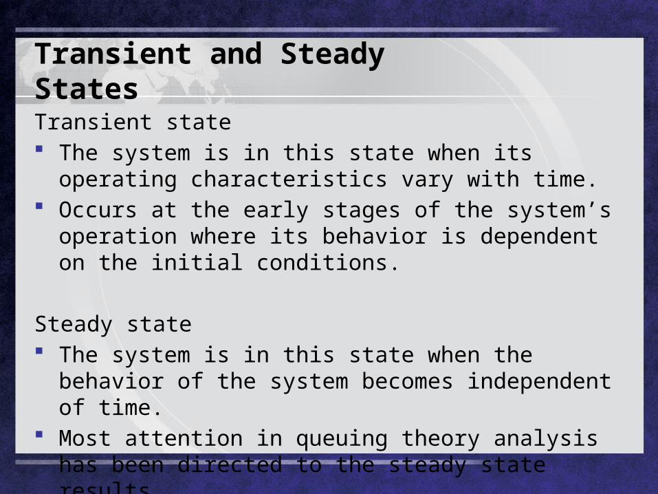
Transient and Steady States
Transient state The system is in this state when its operating
characteristics vary with time. Occurs at the early stages of the system’s operation
where its behavior is dependent on the initial conditions.
Steady state The system is in this state when the behavior of the
system becomes independent of time. Most attention in queuing theory analysis has been
directed to the steady state results.
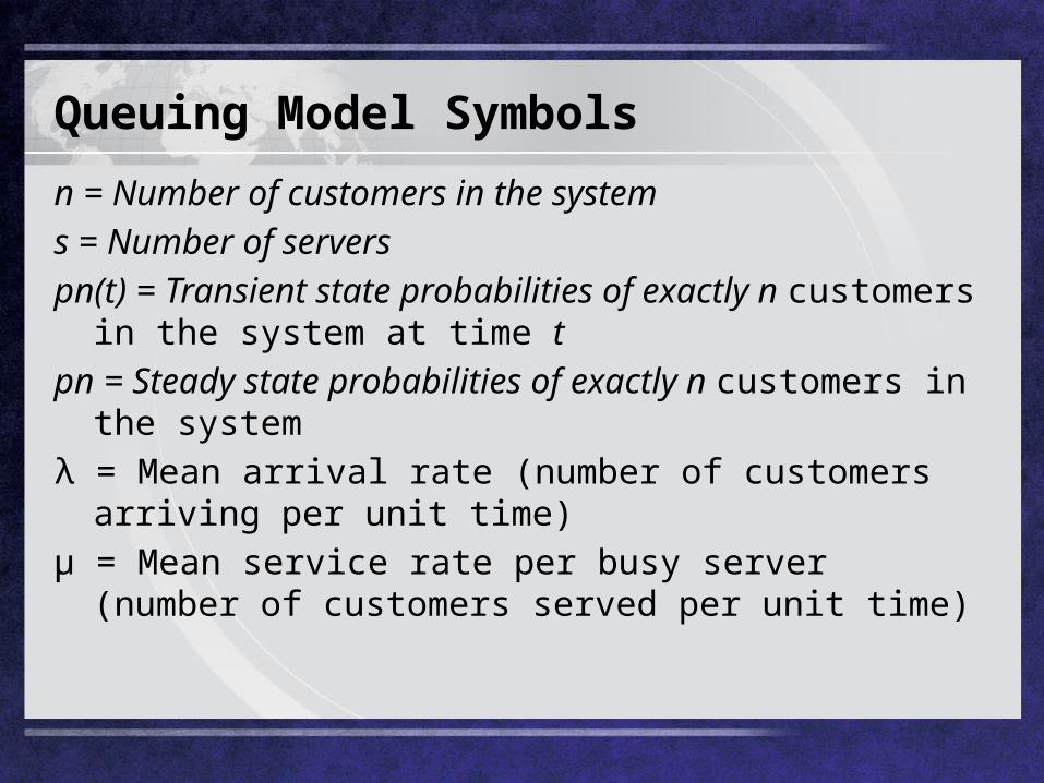
Queuing Model Symbols
n = Number of customers in the system
s = Number of servers
pn(t) = Transient state probabilities of exactly n customers in the system at time t
pn = Steady state probabilities of exactly n customers in the system
λ = Mean arrival rate (number of customers arriving per unit time)
μ = Mean service rate per busy server (number of customers served per unit time)
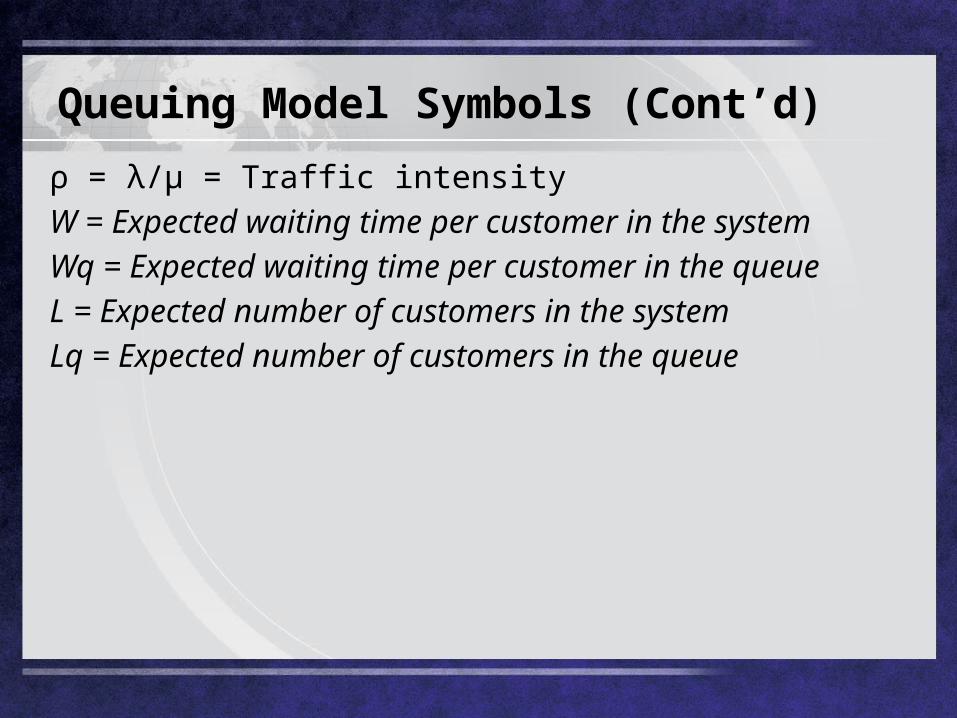
Queuing Model Symbols (Cont’d)
ρ = λ/μ = Traffic intensity
W = Expected waiting time per customer in the system
Wq = Expected waiting time per customer in the queue
L = Expected number of customers in the system
Lq = Expected number of customers in the queue
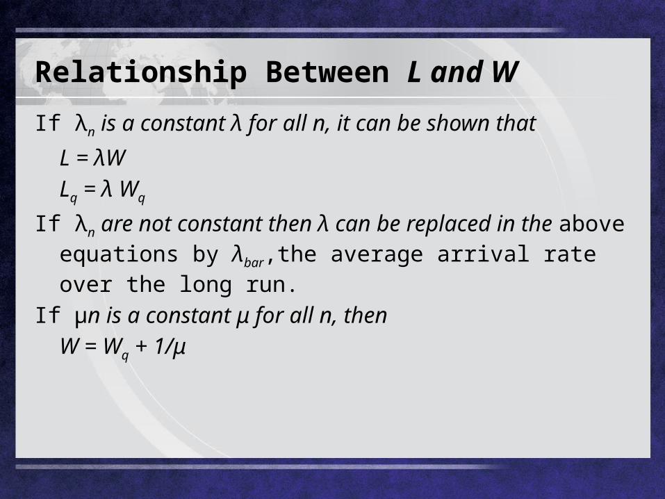
Relationship Between L and W
If λn is a constant λ for all n, it can be shown that
L = λW
Lq = λ Wq
If λn are not constant then λ can be replaced in the above equations by λbar,the average arrival rate over the long run.
If μn is a constant μ for all n, then
W = Wq + 1/μ
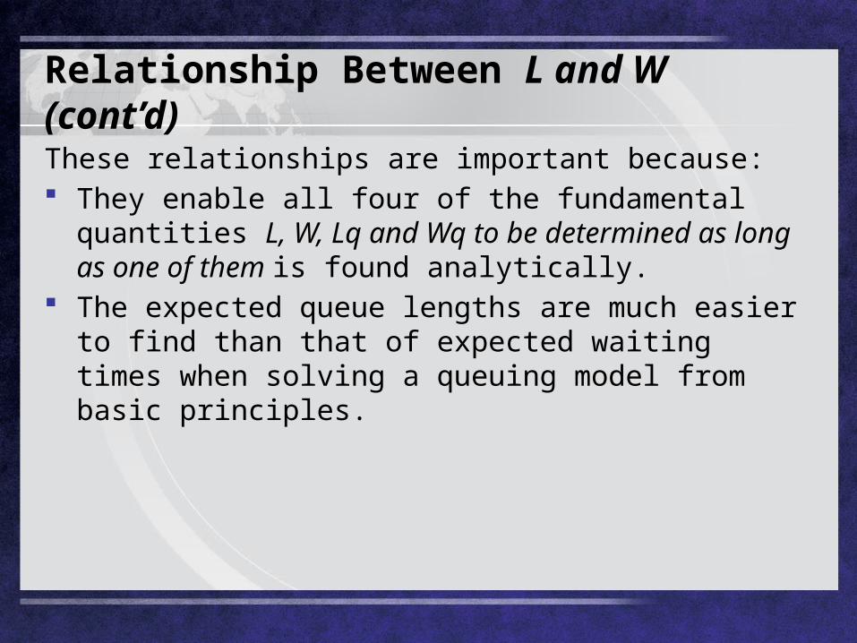
Relationship Between L and W (cont’d)
These relationships are important because: They enable all four of the fundamental quantities L, W,
Lq and Wq to be determined as long as one of them is found analytically.
The expected queue lengths are much easier to find than that of expected waiting times when solving a queuing model from basic principles.
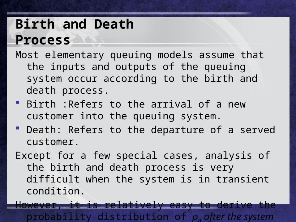
Birth and Death Process
Most elementary queuing models assume that the inputs and outputs of the queuing system occur according to the birth and death process.
Birth :Refers to the arrival of a new customer into the queuing system.
Death: Refers to the departure of a served customer.
Except for a few special cases, analysis of the birth and death process is very difficult when the system is in transient condition.
However, it is relatively easy to derive the probability distribution of pn after the system has reached a steady state condition.
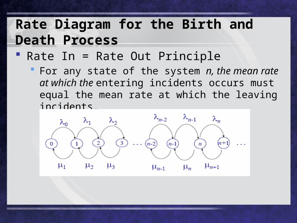
Rate Diagram for the Birth and Death Process Rate In = Rate Out Principle
For any state of the system n, the mean rate at which the entering incidents occurs must equal the mean rate at which the leaving incidents.
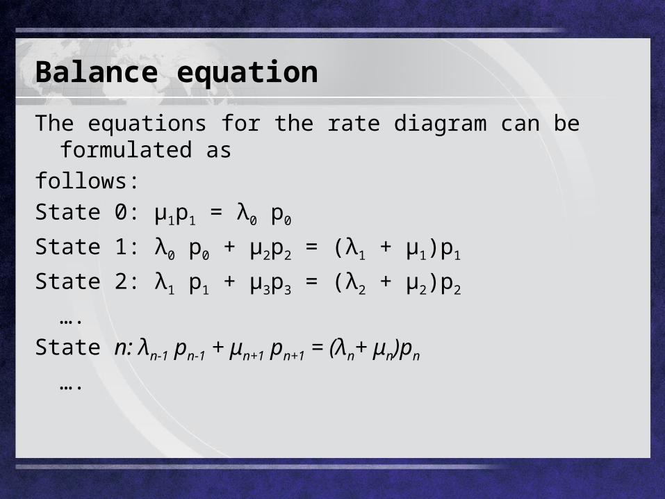
Balance equation
The equations for the rate diagram can be formulated as
follows:
State 0: μ1p1 = λ0 p0
State 1: λ0 p0 + μ2p2 = (λ1 + μ1)p1
State 2: λ1 p1 + μ3p3 = (λ2 + μ2)p2
….
State n: λn-1 pn-1 + μn+1 pn+1 = (λn+ μn)pn
….
Balance equation (cont’d)
0
1
0
1
1 21
1100
1 11
021000
011
021
0123
0123
012
012
01
01
or1
1henceand
1or1obtainwe1Using
:State
:2State
:1State
:0State
pcpc
p
pppp
ppn
pp
pp
pp
nn
nn
n n
n
n nn
nnn n
nn
nnn
cn
Balance equation (cont’d)
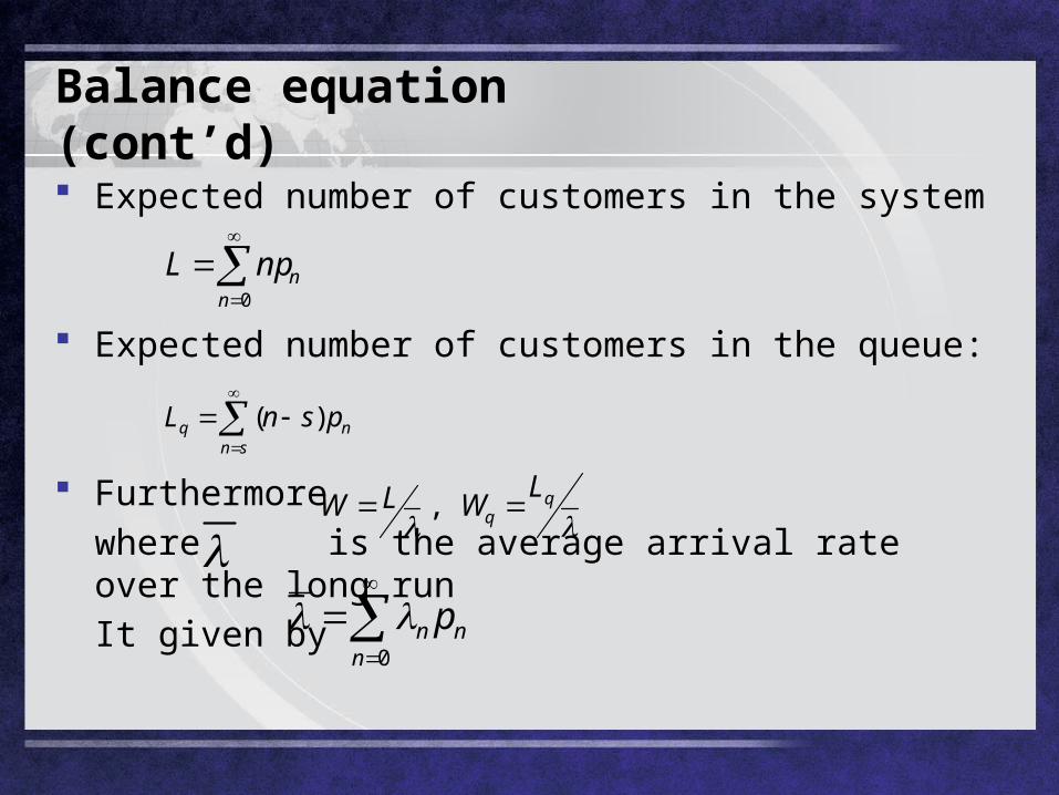
Expected number of customers in the system
Expected number of customers in the queue:
Furthermore
where is the average arrival rate over the long run
It given by
0n
nnpL
sn
nq psnL )(
q
q
LWLW ,
0n
nn p
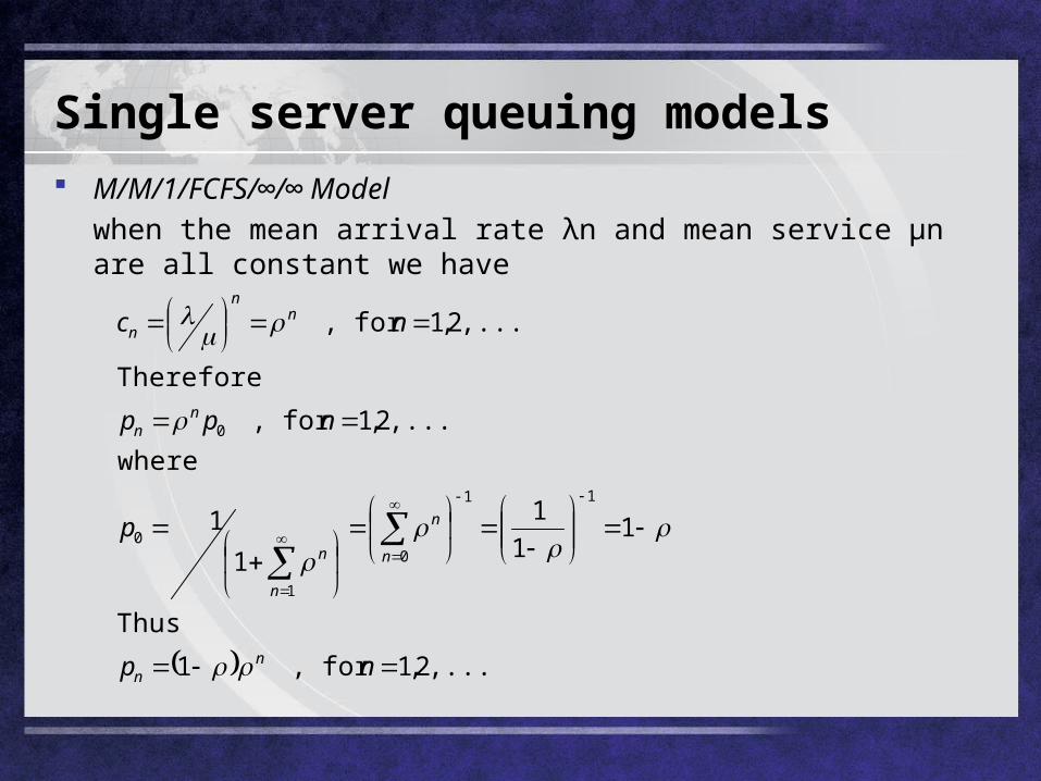
Single server queuing models
M/M/1/FCFS/∞/∞ Model
when the mean arrival rate λn and mean service μn are all constant we have
,...2,1for,1
Thus
11
1
1
1
where
,...2,1for,
Therefore
,...2,1for,
11
0
1
0
0
np
p
npp
nc
nn
n
n
n
n
nn
nn
n
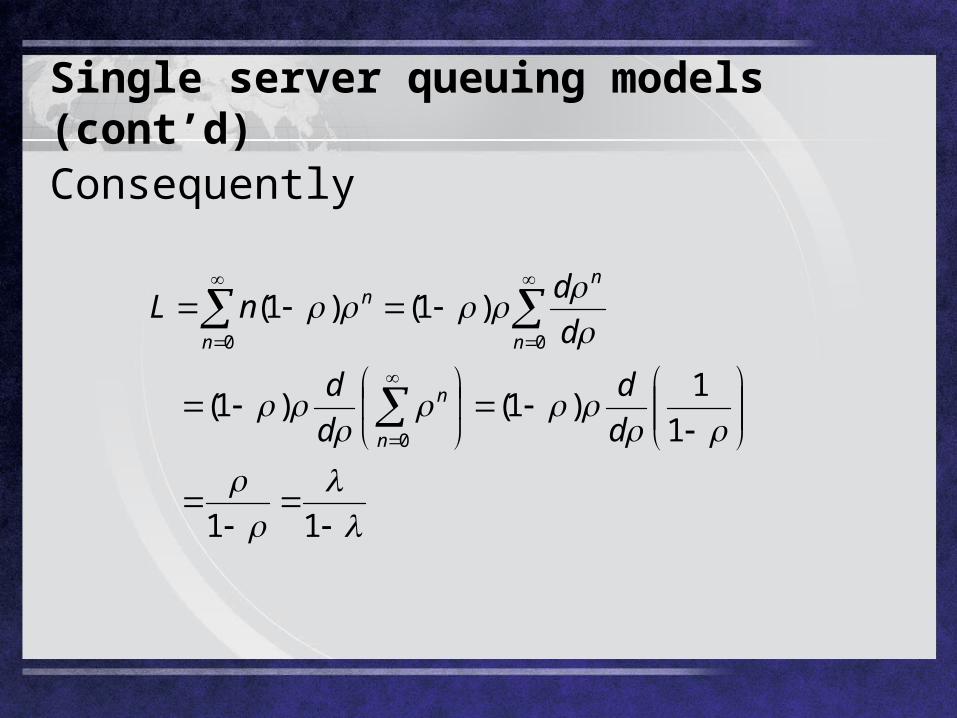
Single server queuing models (cont’d)
Consequently
11
1
1)1()1(
)1()1(
0
00
d
d
d
d
d
dnL
n
n
n
n
n
n
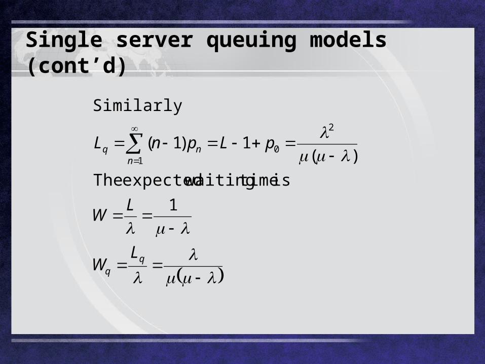
Single server queuing models (cont’d)
nnq
LW
LW
pLpnL
1
istimewaitingexpectedThe
)(1)1(
Similarly2
01
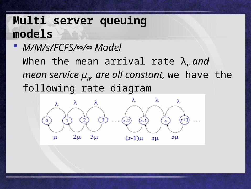
Multi server queuing models
M/M/s/FCFS/∞/∞ Model
When the mean arrival rate λn and mean service μn, are all constant, we have the following rate diagram
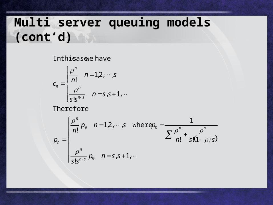
Multi server queuing models (cont’d)
,1,!
1!!
1where,,2,1
!
Therefore
,1,!
,,2,1!
havewecasethisIn
0
00
ssnpss
ssn
psnpn
p
ssnss
snnc
sn
n
sn
n
n
sn
n
n
n
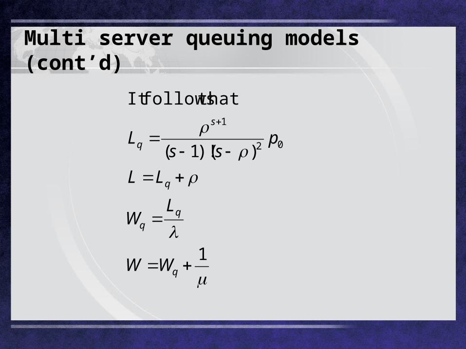
Multi server queuing models (cont’d)
1
)()!1(
thatfollowsIt
02
1
q
q
s
q
WW
LW
LL
pss
L
Some General Comments
Only very simple models allow analytic determination of quantities of interests. That is, closed form solution can be obtained for
simple queuing models only.
Transient versus steady state behavior For some real world queuing systems, the transient
behavior may be of interests to the decision makers.
For the more complex queuing systems, the quantities
of interests may be obtained through simulation.