Embed Size (px)
Citation preview
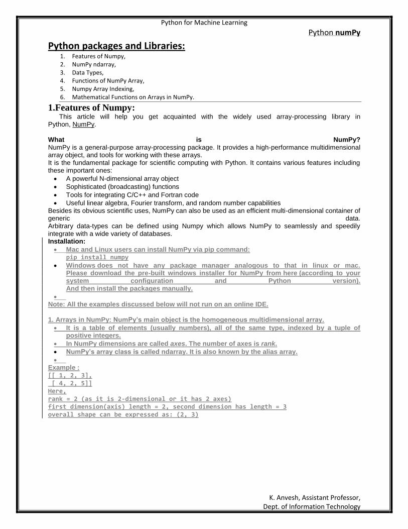
Python for Machine Learning
Python numPy
K. Anvesh, Assistant Professor, Dept. of Information Technology
Python packages and Libraries: 1. Features of Numpy, 2. NumPy ndarray, 3. Data Types, 4. Functions of NumPy Array, 5. Numpy Array Indexing, 6. Mathematical Functions on Arrays in NumPy.
1.Features of Numpy: This article will help you get acquainted with the widely used array-processing library in Python, NumPy. What is NumPy? NumPy is a general-purpose array-processing package. It provides a high-performance multidimensional array object, and tools for working with these arrays. It is the fundamental package for scientific computing with Python. It contains various features including these important ones:
A powerful N-dimensional array object
Sophisticated (broadcasting) functions
Tools for integrating C/C++ and Fortran code
Useful linear algebra, Fourier transform, and random number capabilities Besides its obvious scientific uses, NumPy can also be used as an efficient multi-dimensional container of generic data. Arbitrary data-types can be defined using Numpy which allows NumPy to seamlessly and speedily integrate with a wide variety of databases. Installation:
Mac and Linux users can install NumPy via pip command: pip install numpy
Windows does not have any package manager analogous to that in linux or mac. Please download the pre-built windows installer for NumPy from here (according to your system configuration and Python version). And then install the packages manually.
Note: All the examples discussed below will not run on an online IDE. 1. Arrays in NumPy: NumPy’s main object is the homogeneous multidimensional array.
It is a table of elements (usually numbers), all of the same type, indexed by a tuple of positive integers.
In NumPy dimensions are called axes. The number of axes is rank.
NumPy’s array class is called ndarray. It is also known by the alias array.
Example : [[ 1, 2, 3], [ 4, 2, 5]] Here, rank = 2 (as it is 2-dimensional or it has 2 axes) first dimension(axis) length = 2, second dimension has length = 3 overall shape can be expressed as: (2, 3)
Python for Machine Learning
Python numPy
K. Anvesh, Assistant Professor, Dept. of Information Technology
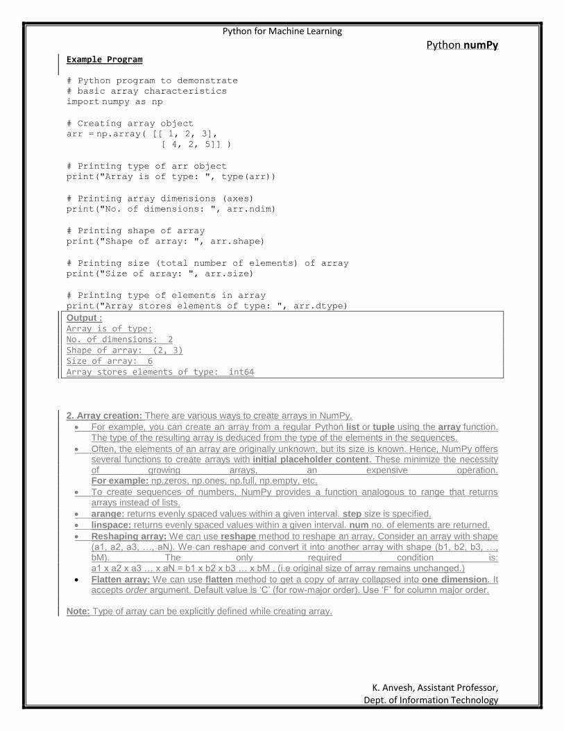
Example Program # Python program to demonstrate # basic array characteristics
import numpy as np
# Creating array object arr = np.array( [[ 1, 2, 3],
[ 4, 2, 5]] )
# Printing type of arr object print("Array is of type: ", type(arr))
# Printing array dimensions (axes) print("No. of dimensions: ", arr.ndim)
# Printing shape of array
print("Shape of array: ", arr.shape)
# Printing size (total number of elements) of array print("Size of array: ", arr.size)
# Printing type of elements in array
print("Array stores elements of type: ", arr.dtype)
Output : Array is of type: No. of dimensions: 2 Shape of array: (2, 3) Size of array: 6 Array stores elements of type: int64
2. Array creation: There are various ways to create arrays in NumPy.
For example, you can create an array from a regular Python list or tuple using the array function. The type of the resulting array is deduced from the type of the elements in the sequences.
Often, the elements of an array are originally unknown, but its size is known. Hence, NumPy offers several functions to create arrays with initial placeholder content. These minimize the necessity of growing arrays, an expensive operation. For example: np.zeros, np.ones, np.full, np.empty, etc.
To create sequences of numbers, NumPy provides a function analogous to range that returns arrays instead of lists.
arange: returns evenly spaced values within a given interval. step size is specified.
linspace: returns evenly spaced values within a given interval. num no. of elements are returned.
Reshaping array: We can use reshape method to reshape an array. Consider an array with shape (a1, a2, a3, …, aN). We can reshape and convert it into another array with shape (b1, b2, b3, …, bM). The only required condition is: a1 x a2 x a3 … x aN = b1 x b2 x b3 … x bM . (i.e original size of array remains unchanged.)
Flatten array: We can use flatten method to get a copy of array collapsed into one dimension. It accepts order argument. Default value is ‘C’ (for row-major order). Use ‘F’ for column major order.
Note: Type of array can be explicitly defined while creating array.
Python for Machine Learning
Python numPy
K. Anvesh, Assistant Professor, Dept. of Information Technology
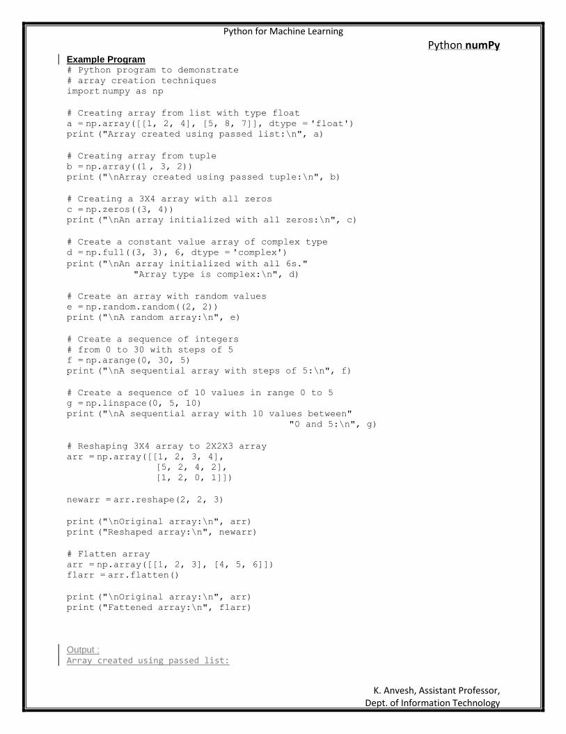
Example Program # Python program to demonstrate
# array creation techniques import numpy as np
# Creating array from list with type float
a = np.array([[1, 2, 4], [5, 8, 7]], dtype = 'float') print ("Array created using passed list:\n", a)
# Creating array from tuple
b = np.array((1 , 3, 2)) print ("\nArray created using passed tuple:\n", b)
# Creating a 3X4 array with all zeros
c = np.zeros((3, 4)) print ("\nAn array initialized with all zeros:\n", c)
# Create a constant value array of complex type
d = np.full((3, 3), 6, dtype = 'complex')
print ("\nAn array initialized with all 6s."
"Array type is complex:\n", d)
# Create an array with random values
e = np.random.random((2, 2)) print ("\nA random array:\n", e)
# Create a sequence of integers
# from 0 to 30 with steps of 5 f = np.arange(0, 30, 5)
print ("\nA sequential array with steps of 5:\n", f)
# Create a sequence of 10 values in range 0 to 5 g = np.linspace(0, 5, 10)
print ("\nA sequential array with 10 values between" "0 and 5:\n", g)
# Reshaping 3X4 array to 2X2X3 array
arr = np.array([[1, 2, 3, 4], [5, 2, 4, 2], [1, 2, 0, 1]])
newarr = arr.reshape(2, 2, 3)
print ("\nOriginal array:\n", arr) print ("Reshaped array:\n", newarr)
# Flatten array
arr = np.array([[1, 2, 3], [4, 5, 6]]) flarr = arr.flatten()
print ("\nOriginal array:\n", arr)
print ("Fattened array:\n", flarr)
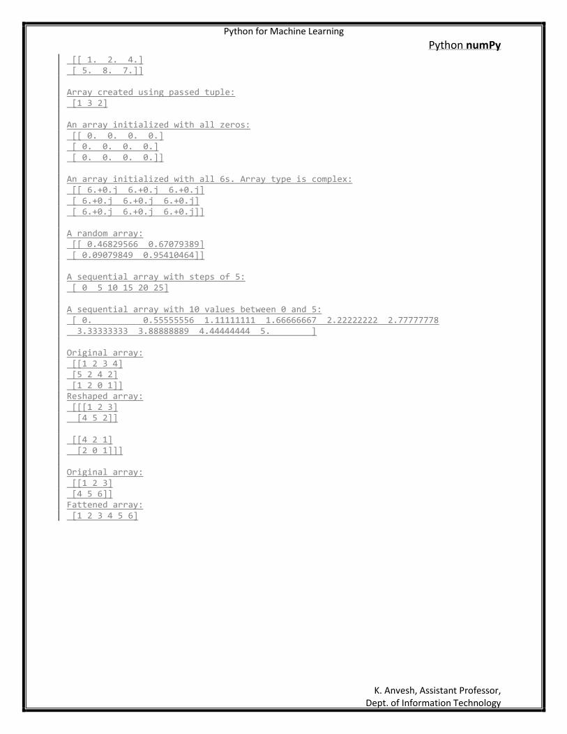
Output : Array created using passed list:
Python for Machine Learning
Python numPy
K. Anvesh, Assistant Professor, Dept. of Information Technology
[[ 1. 2. 4.] [ 5. 8. 7.]] Array created using passed tuple: [1 3 2] An array initialized with all zeros: [[ 0. 0. 0. 0.] [ 0. 0. 0. 0.] [ 0. 0. 0. 0.]] An array initialized with all 6s. Array type is complex: [[ 6.+0.j 6.+0.j 6.+0.j] [ 6.+0.j 6.+0.j 6.+0.j] [ 6.+0.j 6.+0.j 6.+0.j]] A random array: [[ 0.46829566 0.67079389] [ 0.09079849 0.95410464]] A sequential array with steps of 5: [ 0 5 10 15 20 25] A sequential array with 10 values between 0 and 5: [ 0. 0.55555556 1.11111111 1.66666667 2.22222222 2.77777778 3.33333333 3.88888889 4.44444444 5. ] Original array: [[1 2 3 4] [5 2 4 2] [1 2 0 1]] Reshaped array: [[[1 2 3] [4 5 2]] [[4 2 1] [2 0 1]]] Original array: [[1 2 3] [4 5 6]] Fattened array: [1 2 3 4 5 6]
Python for Machine Learning
Python numPy
K. Anvesh, Assistant Professor, Dept. of Information Technology
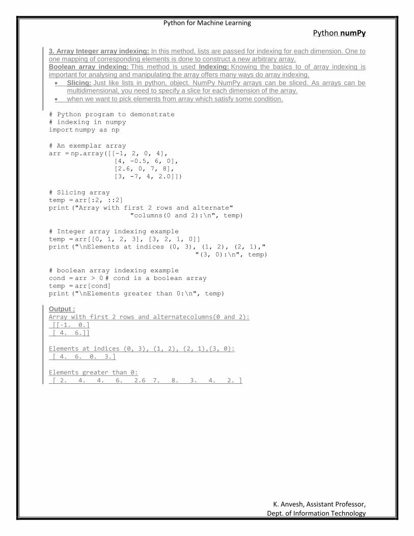
3. Array Integer array indexing: In this method, lists are passed for indexing for each dimension. One to one mapping of corresponding elements is done to construct a new arbitrary array. Boolean array indexing: This method is used Indexing: Knowing the basics to of array indexing is important for analysing and manipulating the array offers many ways do array indexing.
Slicing: Just like lists in python, object. NumPy NumPy arrays can be sliced. As arrays can be multidimensional, you need to specify a slice for each dimension of the array.
when we want to pick elements from array which satisfy some condition. # Python program to demonstrate
# indexing in numpy import numpy as np
# An exemplar array
arr = np.array([[-1, 2, 0, 4], [4, -0.5, 6, 0], [2.6, 0, 7, 8],
[3, -7, 4, 2.0]])
# Slicing array temp = arr[:2, ::2]
print ("Array with first 2 rows and alternate" "columns(0 and 2):\n", temp)
# Integer array indexing example
temp = arr[[0, 1, 2, 3], [3, 2, 1, 0]] print ("\nElements at indices (0, 3), (1, 2), (2, 1),"
"(3, 0):\n", temp)
# boolean array indexing example cond = arr > 0 # cond is a boolean array
temp = arr[cond] print ("\nElements greater than 0:\n", temp)
Output : Array with first 2 rows and alternatecolumns(0 and 2): [[-1. 0.] [ 4. 6.]] Elements at indices (0, 3), (1, 2), (2, 1),(3, 0): [ 4. 6. 0. 3.] Elements greater than 0: [ 2. 4. 4. 6. 2.6 7. 8. 3. 4. 2. ]
Python for Machine Learning
Python numPy
K. Anvesh, Assistant Professor, Dept. of Information Technology
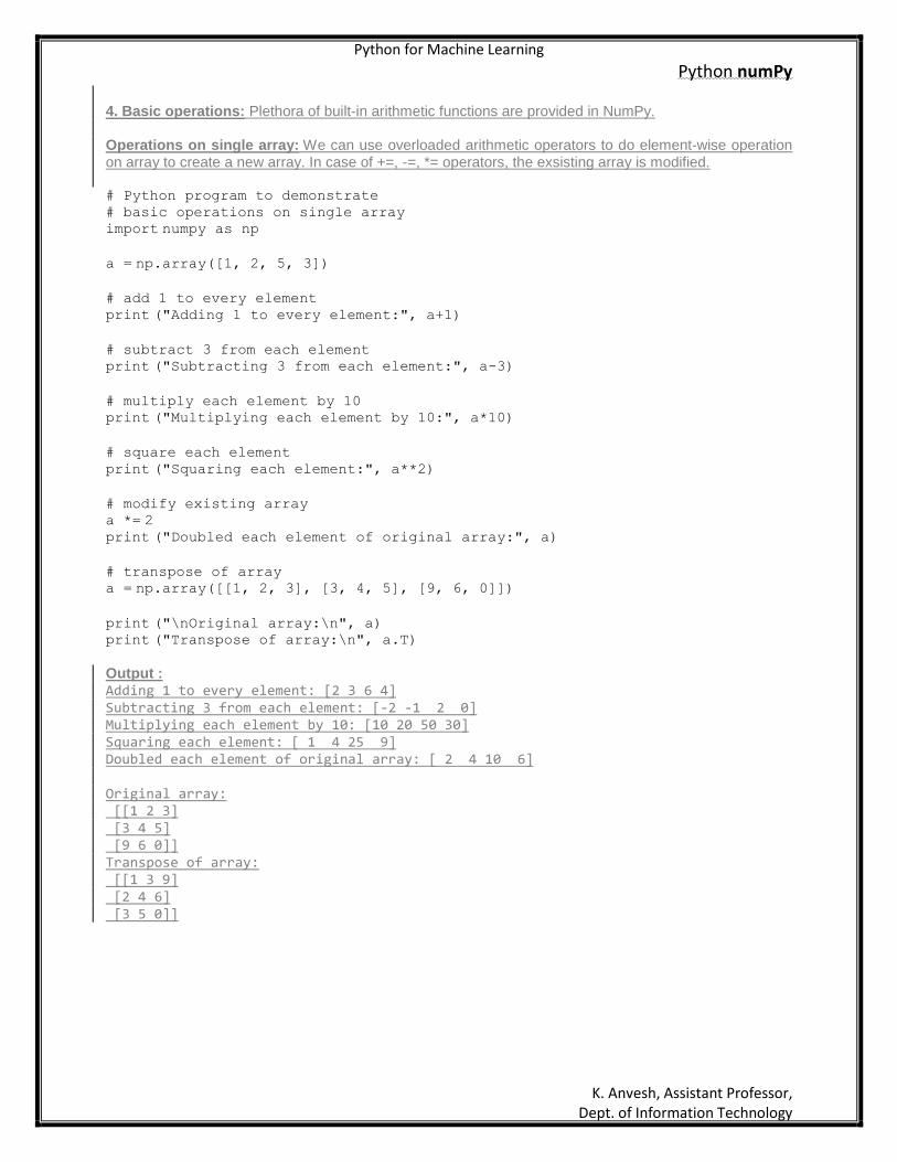
4. Basic operations: Plethora of built-in arithmetic functions are provided in NumPy. Operations on single array: We can use overloaded arithmetic operators to do element-wise operation on array to create a new array. In case of +=, -=, *= operators, the exsisting array is modified. # Python program to demonstrate
# basic operations on single array import numpy as np
a = np.array([1, 2, 5, 3])
# add 1 to every element
print ("Adding 1 to every element:", a+1)
# subtract 3 from each element print ("Subtracting 3 from each element:", a-3)
# multiply each element by 10 print ("Multiplying each element by 10:", a*10)
# square each element
print ("Squaring each element:", a**2)
# modify existing array a *= 2
print ("Doubled each element of original array:", a)
# transpose of array a = np.array([[1, 2, 3], [3, 4, 5], [9, 6, 0]])
print ("\nOriginal array:\n", a) print ("Transpose of array:\n", a.T)
Output : Adding 1 to every element: [2 3 6 4] Subtracting 3 from each element: [-2 -1 2 0] Multiplying each element by 10: [10 20 50 30] Squaring each element: [ 1 4 25 9] Doubled each element of original array: [ 2 4 10 6] Original array: [[1 2 3] [3 4 5] [9 6 0]] Transpose of array: [[1 3 9] [2 4 6] [3 5 0]]
Python for Machine Learning
Python numPy
K. Anvesh, Assistant Professor, Dept. of Information Technology
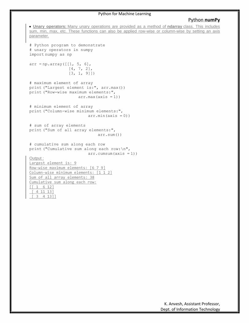
Unary operators: Many unary operations are provided as a method of ndarray class. This includes sum, min, max, etc. These functions can also be applied row-wise or column-wise by setting an axis parameter.
# Python program to demonstrate
# unary operators in numpy import numpy as np
arr = np.array([[1, 5, 6],
[4, 7, 2], [3, 1, 9]])
# maximum element of array
print ("Largest element is:", arr.max()) print ("Row-wise maximum elements:",
arr.max(axis = 1))
# minimum element of array print ("Column-wise minimum elements:",
arr.min(axis = 0))
# sum of array elements print ("Sum of all array elements:",
arr.sum())
# cumulative sum along each row print ("Cumulative sum along each row:\n",
arr.cumsum(axis = 1))
Output : Largest element is: 9 Row-wise maximum elements: [6 7 9] Column-wise minimum elements: [1 1 2] Sum of all array elements: 38 Cumulative sum along each row: [[ 1 6 12] [ 4 11 13] [ 3 4 13]]
Python for Machine Learning
Python numPy
K. Anvesh, Assistant Professor, Dept. of Information Technology
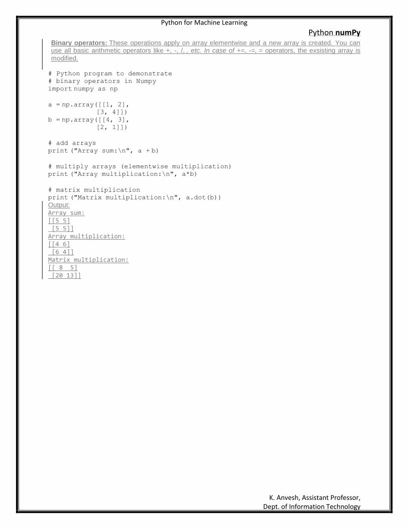
Binary operators: These operations apply on array elementwise and a new array is created. You can use all basic arithmetic operators like +, -, /, , etc. In case of +=, -=, = operators, the exsisting array is modified.
# Python program to demonstrate # binary operators in Numpy
import numpy as np
a = np.array([[1, 2], [3, 4]])
b = np.array([[4, 3], [2, 1]])
# add arrays
print ("Array sum:\n", a + b)
# multiply arrays (elementwise multiplication) print ("Array multiplication:\n", a*b)
# matrix multiplication print ("Matrix multiplication:\n", a.dot(b))
Output: Array sum: [[5 5] [5 5]] Array multiplication: [[4 6] [6 4]] Matrix multiplication: [[ 8 5] [20 13]]
Python for Machine Learning
Python numPy
K. Anvesh, Assistant Professor, Dept. of Information Technology
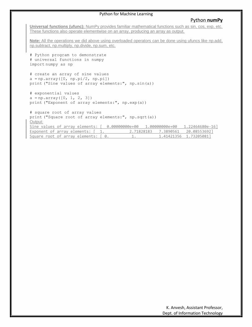
Universal functions (ufunc): NumPy provides familiar mathematical functions such as sin, cos, exp, etc. These functions also operate elementwise on an array, producing an array as output.
Note: All the operations we did above using overloaded operators can be done using ufuncs like np.add, np.subtract, np.multiply, np.divide, np.sum, etc. # Python program to demonstrate
# universal functions in numpy import numpy as np
# create an array of sine values
a = np.array([0, np.pi/2, np.pi]) print ("Sine values of array elements:", np.sin(a))
# exponential values a = np.array([0, 1, 2, 3]) print ("Exponent of array elements:", np.exp(a))
# square root of array values print ("Square root of array elements:", np.sqrt(a))
Output: Sine values of array elements: [ 0.00000000e+00 1.00000000e+00 1.22464680e-16] Exponent of array elements: [ 1. 2.71828183 7.3890561 20.08553692] Square root of array elements: [ 0. 1. 1.41421356 1.73205081]
Python for Machine Learning
Python numPy
K. Anvesh, Assistant Professor, Dept. of Information Technology
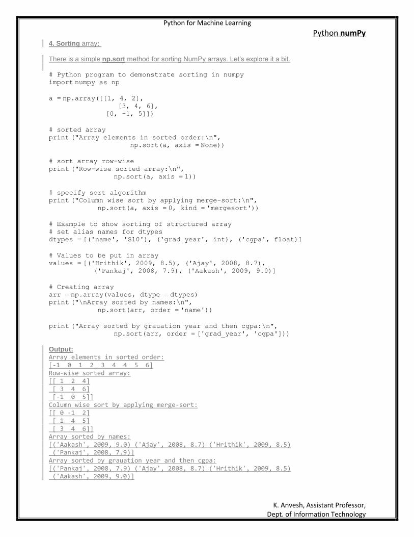
4. Sorting array: There is a simple np.sort method for sorting NumPy arrays. Let’s explore it a bit. # Python program to demonstrate sorting in numpy import numpy as np
a = np.array([[1, 4, 2],
[3, 4, 6], [0, -1, 5]])
# sorted array
print ("Array elements in sorted order:\n", np.sort(a, axis = None))
# sort array row-wise
print ("Row-wise sorted array:\n", np.sort(a, axis = 1))
# specify sort algorithm print ("Column wise sort by applying merge-sort:\n", np.sort(a, axis = 0, kind = 'mergesort'))
# Example to show sorting of structured array # set alias names for dtypes dtypes = [('name', 'S10'), ('grad_year', int), ('cgpa', float)]
# Values to be put in array values = [('Hrithik', 2009, 8.5), ('Ajay', 2008, 8.7), ('Pankaj', 2008, 7.9), ('Aakash', 2009, 9.0)]
# Creating array arr = np.array(values, dtype = dtypes) print ("\nArray sorted by names:\n",
np.sort(arr, order = 'name'))
print ("Array sorted by grauation year and then cgpa:\n", np.sort(arr, order = ['grad_year', 'cgpa']))
Output: Array elements in sorted order: [-1 0 1 2 3 4 4 5 6] Row-wise sorted array: [[ 1 2 4] [ 3 4 6] [-1 0 5]] Column wise sort by applying merge-sort: [[ 0 -1 2] [ 1 4 5] [ 3 4 6]] Array sorted by names: [('Aakash', 2009, 9.0) ('Ajay', 2008, 8.7) ('Hrithik', 2009, 8.5) ('Pankaj', 2008, 7.9)] Array sorted by grauation year and then cgpa: [('Pankaj', 2008, 7.9) ('Ajay', 2008, 8.7) ('Hrithik', 2009, 8.5) ('Aakash', 2009, 9.0)]
Python for Machine Learning
Python numPy
K. Anvesh, Assistant Professor, Dept. of Information Technology
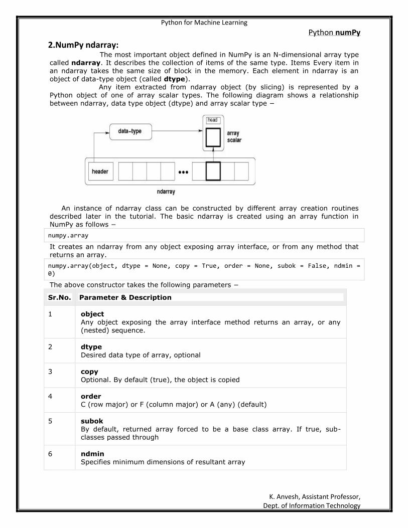
2.NumPy ndarray: The most important object defined in NumPy is an N-dimensional array type
called ndarray. It describes the collection of items of the same type. Items Every item in
an ndarray takes the same size of block in the memory. Each element in ndarray is an
object of data-type object (called dtype).
Any item extracted from ndarray object (by slicing) is represented by a
Python object of one of array scalar types. The following diagram shows a relationship
between ndarray, data type object (dtype) and array scalar type −
An instance of ndarray class can be constructed by different array creation routines
described later in the tutorial. The basic ndarray is created using an array function in
NumPy as follows −
numpy.array
It creates an ndarray from any object exposing array interface, or from any method that
returns an array.
numpy.array(object, dtype = None, copy = True, order = None, subok = False, ndmin = 0)
The above constructor takes the following parameters −
Sr.No. Parameter & Description
1 object
Any object exposing the array interface method returns an array, or any
(nested) sequence.
2 dtype
Desired data type of array, optional
3 copy
Optional. By default (true), the object is copied
4 order
C (row major) or F (column major) or A (any) (default)
5 subok
By default, returned array forced to be a base class array. If true, sub-
classes passed through
6 ndmin
Specifies minimum dimensions of resultant array
Python for Machine Learning
Python numPy
K. Anvesh, Assistant Professor, Dept. of Information Technology
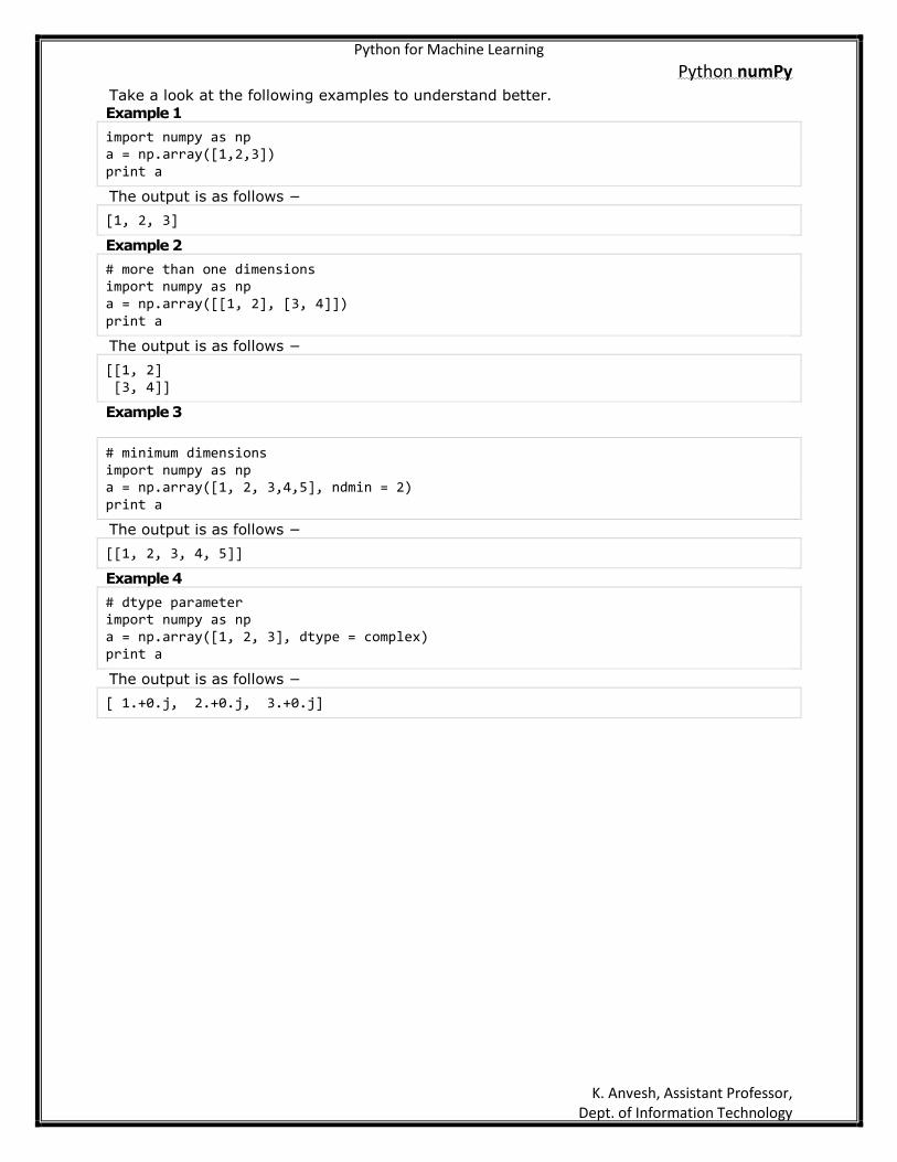
Take a look at the following examples to understand better.
Example 1
import numpy as np a = np.array([1,2,3]) print a
The output is as follows −
[1, 2, 3]
Example 2
# more than one dimensions import numpy as np a = np.array([[1, 2], [3, 4]]) print a
The output is as follows −
[[1, 2] [3, 4]]
Example 3
# minimum dimensions import numpy as np a = np.array([1, 2, 3,4,5], ndmin = 2) print a
The output is as follows −
[[1, 2, 3, 4, 5]]
Example 4
# dtype parameter import numpy as np a = np.array([1, 2, 3], dtype = complex) print a
The output is as follows −
[ 1.+0.j, 2.+0.j, 3.+0.j]
Python for Machine Learning
Python numPy
K. Anvesh, Assistant Professor, Dept. of Information Technology
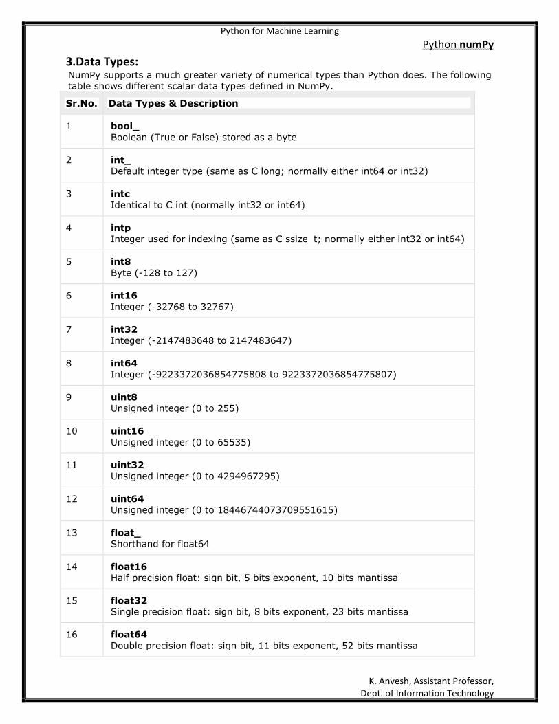
3.Data Types: NumPy supports a much greater variety of numerical types than Python does. The following
table shows different scalar data types defined in NumPy.
Sr.No. Data Types & Description
1 bool_
Boolean (True or False) stored as a byte
2 int_
Default integer type (same as C long; normally either int64 or int32)
3 intc
Identical to C int (normally int32 or int64)
4 intp
Integer used for indexing (same as C ssize_t; normally either int32 or int64)
5 int8
Byte (-128 to 127)
6 int16
Integer (-32768 to 32767)
7 int32
Integer (-2147483648 to 2147483647)
8 int64
Integer (-9223372036854775808 to 9223372036854775807)
9 uint8
Unsigned integer (0 to 255)
10 uint16
Unsigned integer (0 to 65535)
11 uint32
Unsigned integer (0 to 4294967295)
12 uint64
Unsigned integer (0 to 18446744073709551615)
13 float_
Shorthand for float64
14 float16
Half precision float: sign bit, 5 bits exponent, 10 bits mantissa
15 float32
Single precision float: sign bit, 8 bits exponent, 23 bits mantissa
16 float64
Double precision float: sign bit, 11 bits exponent, 52 bits mantissa
Python for Machine Learning
Python numPy
K. Anvesh, Assistant Professor, Dept. of Information Technology
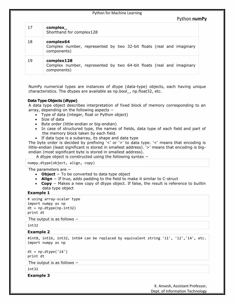
17 complex_
Shorthand for complex128
18 complex64
Complex number, represented by two 32-bit floats (real and imaginary
components)
19 complex128
Complex number, represented by two 64-bit floats (real and imaginary
components)
NumPy numerical types are instances of dtype (data-type) objects, each having unique
characteristics. The dtypes are available as np.bool_, np.float32, etc.
Data Type Objects (dtype)
A data type object describes interpretation of fixed block of memory corresponding to an
array, depending on the following aspects −
Type of data (integer, float or Python object)
Size of data
Byte order (little-endian or big-endian)
In case of structured type, the names of fields, data type of each field and part of
the memory block taken by each field.
If data type is a subarray, its shape and data type
The byte order is decided by prefixing '<' or '>' to data type. '<' means that encoding is
little-endian (least significant is stored in smallest address). '>' means that encoding is big-
endian (most significant byte is stored in smallest address).
A dtype object is constructed using the following syntax −
numpy.dtype(object, align, copy)
The parameters are −
Object − To be converted to data type object
Align − If true, adds padding to the field to make it similar to C-struct
Copy − Makes a new copy of dtype object. If false, the result is reference to builtin
data type object
Example 1
# using array-scalar type import numpy as np dt = np.dtype(np.int32) print dt
The output is as follows −
int32
Example 2
#int8, int16, int32, int64 can be replaced by equivalent string 'i1', 'i2','i4', etc. import numpy as np dt = np.dtype('i4') print dt
The output is as follows −
int32
Example 3
Python for Machine Learning
Python numPy
K. Anvesh, Assistant Professor, Dept. of Information Technology
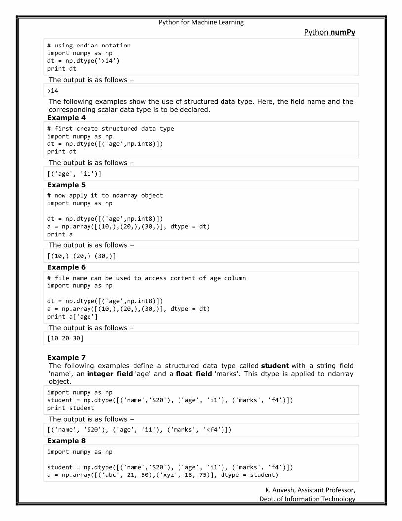
# using endian notation import numpy as np dt = np.dtype('>i4') print dt
The output is as follows −
>i4
The following examples show the use of structured data type. Here, the field name and the
corresponding scalar data type is to be declared.
Example 4
# first create structured data type import numpy as np dt = np.dtype([('age',np.int8)]) print dt
The output is as follows −
[('age', 'i1')]
Example 5
# now apply it to ndarray object import numpy as np dt = np.dtype([('age',np.int8)]) a = np.array([(10,),(20,),(30,)], dtype = dt) print a
The output is as follows −
[(10,) (20,) (30,)]
Example 6
# file name can be used to access content of age column import numpy as np dt = np.dtype([('age',np.int8)]) a = np.array([(10,),(20,),(30,)], dtype = dt) print a['age']
The output is as follows −
[10 20 30]
Example 7
The following examples define a structured data type called student with a string field
'name', an integer field 'age' and a float field 'marks'. This dtype is applied to ndarray
object.
import numpy as np student = np.dtype([('name','S20'), ('age', 'i1'), ('marks', 'f4')]) print student
The output is as follows −
[('name', 'S20'), ('age', 'i1'), ('marks', '<f4')])
Example 8
import numpy as np student = np.dtype([('name','S20'), ('age', 'i1'), ('marks', 'f4')]) a = np.array([('abc', 21, 50),('xyz', 18, 75)], dtype = student)
Python for Machine Learning
Python numPy
K. Anvesh, Assistant Professor, Dept. of Information Technology
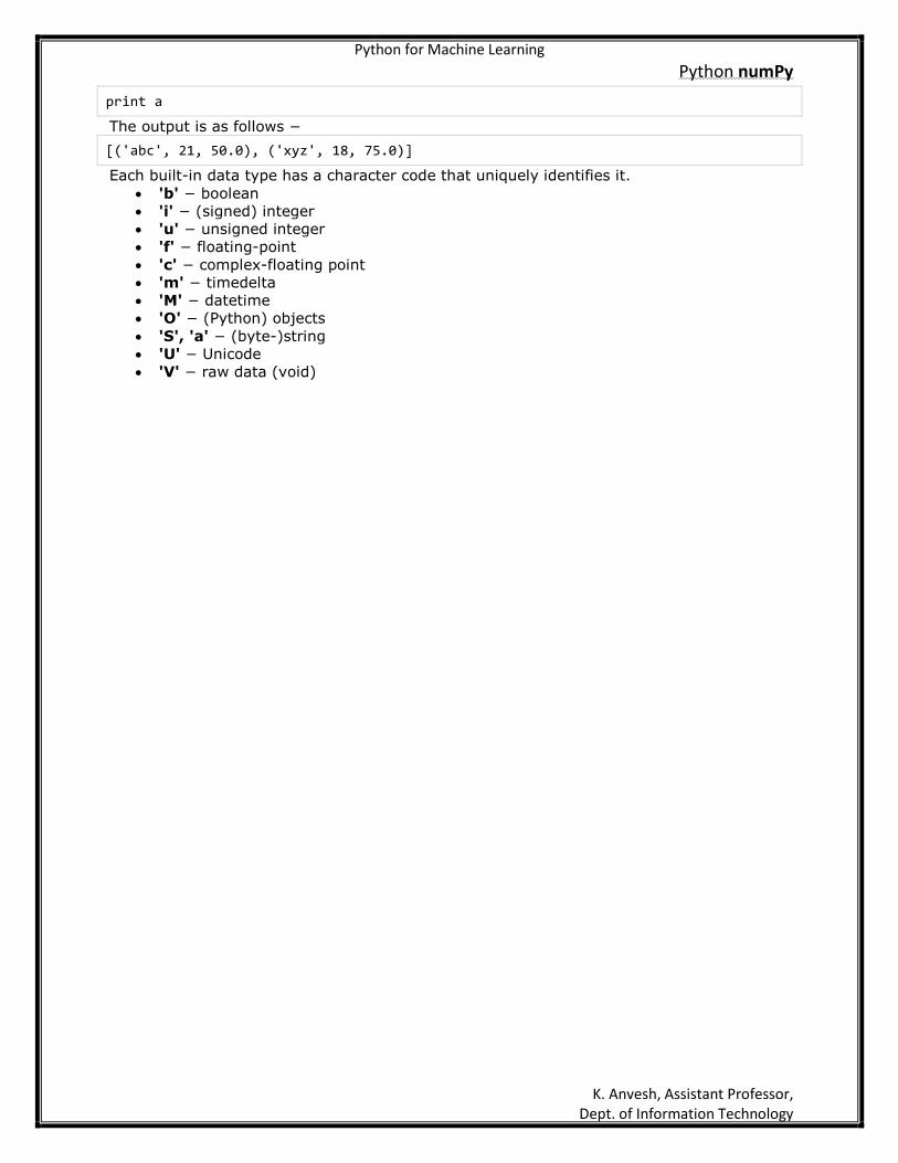
print a
The output is as follows −
[('abc', 21, 50.0), ('xyz', 18, 75.0)]
Each built-in data type has a character code that uniquely identifies it.
'b' − boolean
'i' − (signed) integer
'u' − unsigned integer
'f' − floating-point
'c' − complex-floating point
'm' − timedelta
'M' − datetime
'O' − (Python) objects
'S', 'a' − (byte-)string
'U' − Unicode
'V' − raw data (void)
Python for Machine Learning
Python numPy
K. Anvesh, Assistant Professor, Dept. of Information Technology
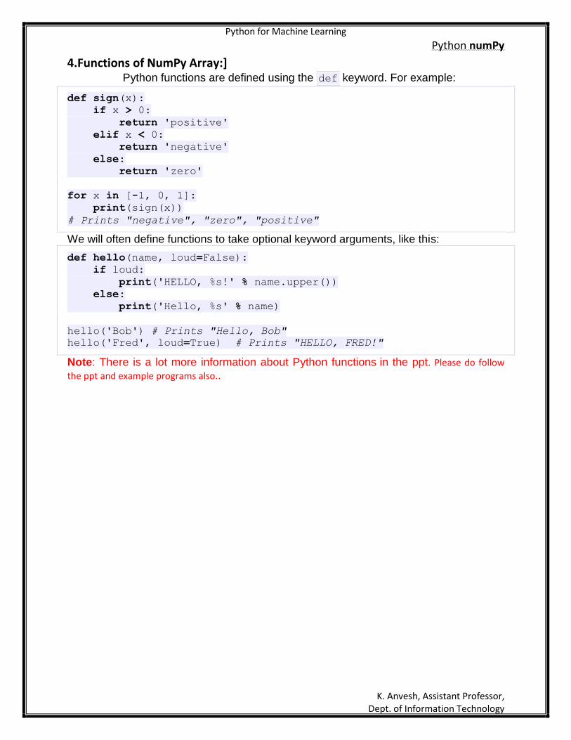
4.Functions of NumPy Array:] Python functions are defined using the def keyword. For example:
def sign(x):
if x > 0:
return 'positive'
elif x < 0:
return 'negative'
else:
return 'zero'
for x in [-1, 0, 1]:
print(sign(x))
# Prints "negative", "zero", "positive"
We will often define functions to take optional keyword arguments, like this:
def hello(name, loud=False):
if loud:
print('HELLO, %s!' % name.upper())
else:
print('Hello, %s' % name)
hello('Bob') # Prints "Hello, Bob"
hello('Fred', loud=True) # Prints "HELLO, FRED!"
Note: There is a lot more information about Python functions in the ppt. Please do follow
the ppt and example programs also..
Python for Machine Learning
Python numPy
K. Anvesh, Assistant Professor, Dept. of Information Technology
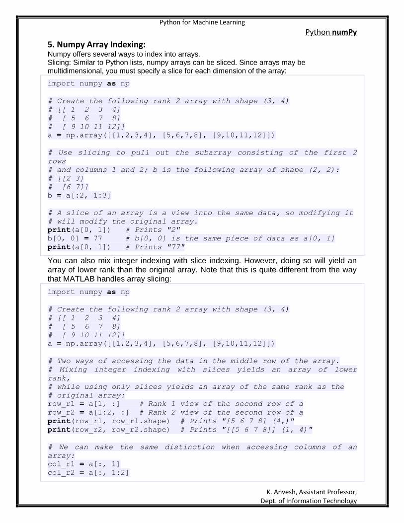
5. Numpy Array Indexing: Numpy offers several ways to index into arrays. Slicing: Similar to Python lists, numpy arrays can be sliced. Since arrays may be multidimensional, you must specify a slice for each dimension of the array:
import numpy as np
# Create the following rank 2 array with shape (3, 4)
# [[ 1 2 3 4]
# [ 5 6 7 8]
# [ 9 10 11 12]]
a = np.array([[1,2,3,4], [5,6,7,8], [9,10,11,12]])
# Use slicing to pull out the subarray consisting of the first 2
rows
# and columns 1 and 2; b is the following array of shape (2, 2):
# [[2 3]
# [6 7]]
b = a[:2, 1:3]
# A slice of an array is a view into the same data, so modifying it
# will modify the original array.
print(a[0, 1]) # Prints "2"
b[0, 0] = 77 # b[0, 0] is the same piece of data as a[0, 1]
print(a[0, 1]) # Prints "77"
You can also mix integer indexing with slice indexing. However, doing so will yield an array of lower rank than the original array. Note that this is quite different from the way that MATLAB handles array slicing:
import numpy as np
# Create the following rank 2 array with shape (3, 4)
# [[ 1 2 3 4]
# [ 5 6 7 8]
# [ 9 10 11 12]]
a = np.array([[1,2,3,4], [5,6,7,8], [9,10,11,12]])
# Two ways of accessing the data in the middle row of the array.
# Mixing integer indexing with slices yields an array of lower
rank,
# while using only slices yields an array of the same rank as the
# original array:
row_r1 = a[1, :] # Rank 1 view of the second row of a
row_r2 = a[1:2, :] # Rank 2 view of the second row of a
print(row_r1, row_r1.shape) # Prints "[5 6 7 8] (4,)"
print(row_r2, row_r2.shape) # Prints "[[5 6 7 8]] (1, 4)"
# We can make the same distinction when accessing columns of an
array:
col_r1 = a[:, 1]
col_r2 = a[:, 1:2]
Python for Machine Learning
Python numPy
K. Anvesh, Assistant Professor, Dept. of Information Technology
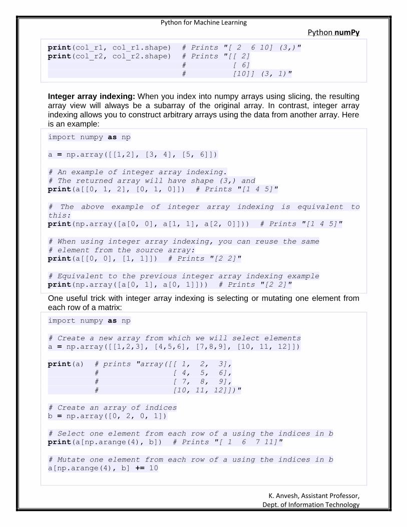
print(col_r1, col_r1.shape) # Prints "[ 2 6 10] (3,)"
print(col_r2, col_r2.shape) # Prints "[[ 2]
# [ 6]
# [10]] (3, 1)"
Integer array indexing: When you index into numpy arrays using slicing, the resulting array view will always be a subarray of the original array. In contrast, integer array indexing allows you to construct arbitrary arrays using the data from another array. Here is an example:
import numpy as np
a = np.array([[1,2], [3, 4], [5, 6]])
# An example of integer array indexing.
# The returned array will have shape (3,) and
print(a[[0, 1, 2], [0, 1, 0]]) # Prints "[1 4 5]"
# The above example of integer array indexing is equivalent to
this:
print(np.array([a[0, 0], a[1, 1], a[2, 0]])) # Prints "[1 4 5]"
# When using integer array indexing, you can reuse the same
# element from the source array:
print(a[[0, 0], [1, 1]]) # Prints "[2 2]"
# Equivalent to the previous integer array indexing example
print(np.array([a[0, 1], a[0, 1]])) # Prints "[2 2]"
One useful trick with integer array indexing is selecting or mutating one element from each row of a matrix:
import numpy as np
# Create a new array from which we will select elements
a = np.array([[1,2,3], [4,5,6], [7,8,9], [10, 11, 12]])
print(a) # prints "array([[ 1, 2, 3],
# [ 4, 5, 6],
# [ 7, 8, 9],
# [10, 11, 12]])"
# Create an array of indices
b = np.array([0, 2, 0, 1])
# Select one element from each row of a using the indices in b
print(a[np.arange(4), b]) # Prints "[ 1 6 7 11]"
# Mutate one element from each row of a using the indices in b
a[np.arange(4), b] += 10
Python for Machine Learning
Python numPy
K. Anvesh, Assistant Professor, Dept. of Information Technology
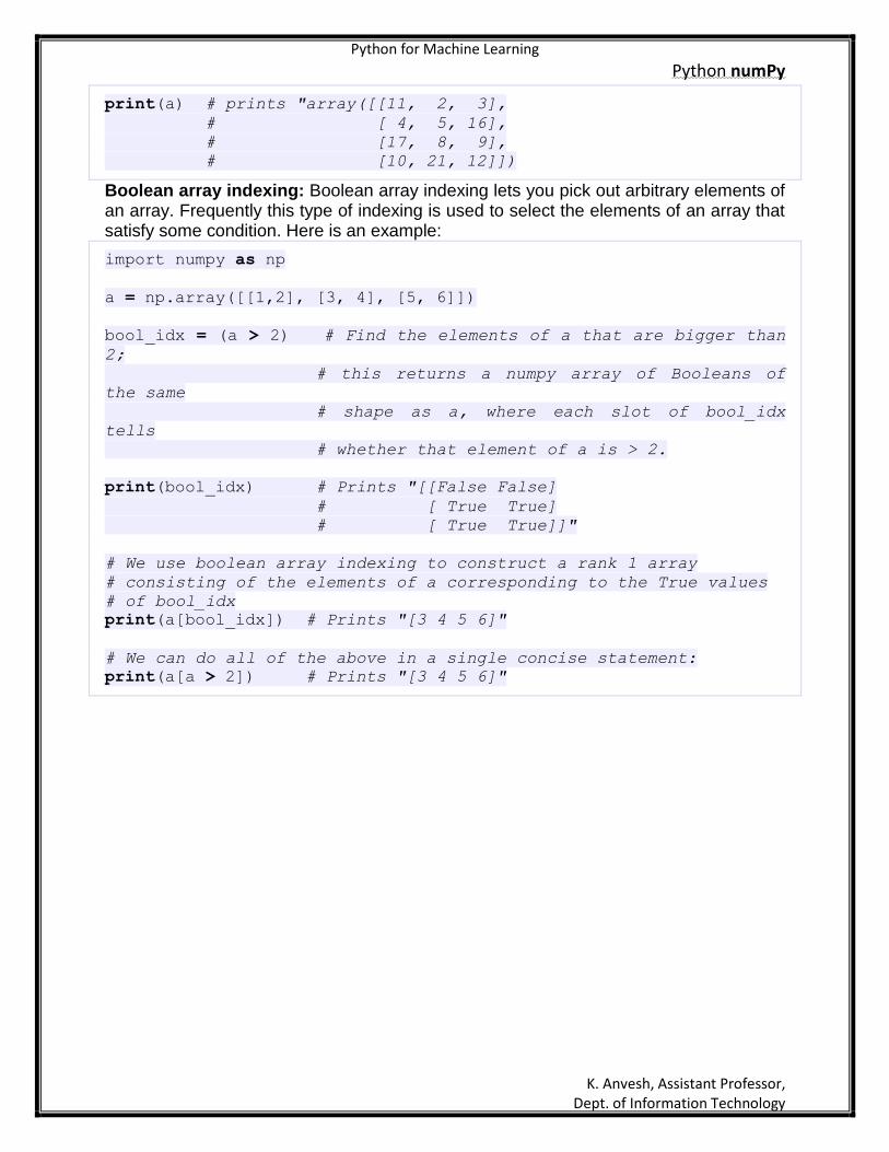
print(a) # prints "array([[11, 2, 3],
# [ 4, 5, 16],
# [17, 8, 9],
# [10, 21, 12]])
Boolean array indexing: Boolean array indexing lets you pick out arbitrary elements of an array. Frequently this type of indexing is used to select the elements of an array that satisfy some condition. Here is an example:
import numpy as np
a = np.array([[1,2], [3, 4], [5, 6]])
bool_idx = (a > 2) # Find the elements of a that are bigger than
2;
# this returns a numpy array of Booleans of
the same
# shape as a, where each slot of bool_idx
tells
# whether that element of a is > 2.
print(bool_idx) # Prints "[[False False]
# [ True True]
# [ True True]]"
# We use boolean array indexing to construct a rank 1 array
# consisting of the elements of a corresponding to the True values
# of bool_idx
print(a[bool_idx]) # Prints "[3 4 5 6]"
# We can do all of the above in a single concise statement:
print(a[a > 2]) # Prints "[3 4 5 6]"
Python for Machine Learning
Python numPy
K. Anvesh, Assistant Professor, Dept. of Information Technology
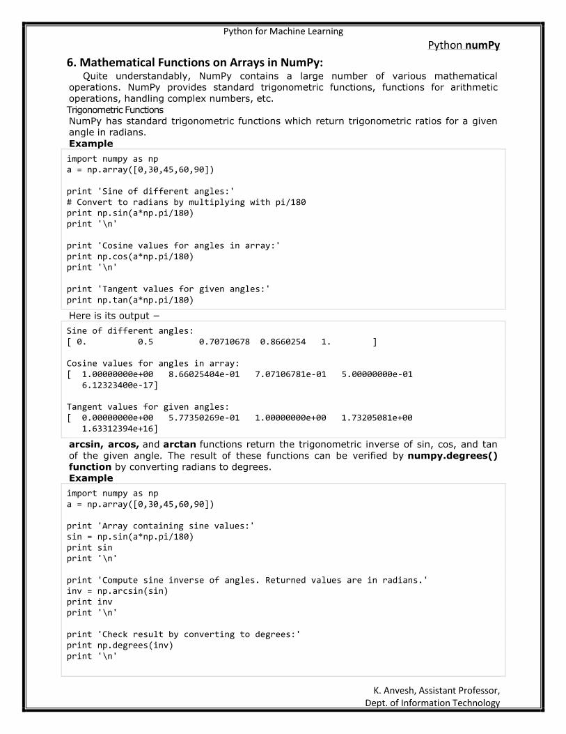
6. Mathematical Functions on Arrays in NumPy: Quite understandably, NumPy contains a large number of various mathematical
operations. NumPy provides standard trigonometric functions, functions for arithmetic
operations, handling complex numbers, etc.
Trigonometric Functions
NumPy has standard trigonometric functions which return trigonometric ratios for a given
angle in radians.
Example
import numpy as np a = np.array([0,30,45,60,90]) print 'Sine of different angles:' # Convert to radians by multiplying with pi/180 print np.sin(a*np.pi/180) print '\n' print 'Cosine values for angles in array:' print np.cos(a*np.pi/180) print '\n' print 'Tangent values for given angles:' print np.tan(a*np.pi/180)
Here is its output −
Sine of different angles: [ 0. 0.5 0.70710678 0.8660254 1. ] Cosine values for angles in array: [ 1.00000000e+00 8.66025404e-01 7.07106781e-01 5.00000000e-01 6.12323400e-17] Tangent values for given angles: [ 0.00000000e+00 5.77350269e-01 1.00000000e+00 1.73205081e+00 1.63312394e+16]
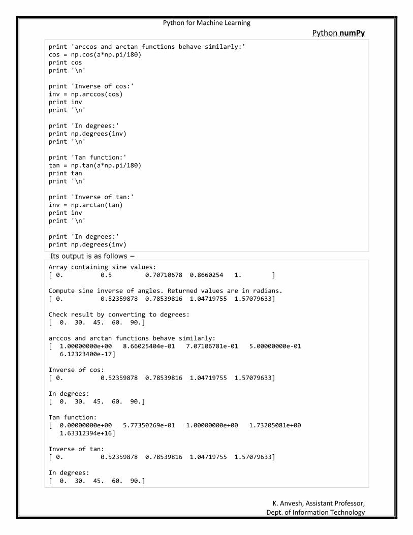
arcsin, arcos, and arctan functions return the trigonometric inverse of sin, cos, and tan
of the given angle. The result of these functions can be verified by numpy.degrees()
function by converting radians to degrees.
Example
import numpy as np a = np.array([0,30,45,60,90]) print 'Array containing sine values:' sin = np.sin(a*np.pi/180) print sin print '\n' print 'Compute sine inverse of angles. Returned values are in radians.' inv = np.arcsin(sin) print inv print '\n' print 'Check result by converting to degrees:' print np.degrees(inv) print '\n'
Python for Machine Learning
Python numPy
K. Anvesh, Assistant Professor, Dept. of Information Technology
print 'arccos and arctan functions behave similarly:' cos = np.cos(a*np.pi/180) print cos print '\n' print 'Inverse of cos:' inv = np.arccos(cos) print inv print '\n' print 'In degrees:' print np.degrees(inv) print '\n' print 'Tan function:' tan = np.tan(a*np.pi/180) print tan print '\n' print 'Inverse of tan:' inv = np.arctan(tan) print inv print '\n' print 'In degrees:' print np.degrees(inv)
Its output is as follows −
Array containing sine values: [ 0. 0.5 0.70710678 0.8660254 1. ] Compute sine inverse of angles. Returned values are in radians. [ 0. 0.52359878 0.78539816 1.04719755 1.57079633] Check result by converting to degrees: [ 0. 30. 45. 60. 90.] arccos and arctan functions behave similarly: [ 1.00000000e+00 8.66025404e-01 7.07106781e-01 5.00000000e-01 6.12323400e-17] Inverse of cos: [ 0. 0.52359878 0.78539816 1.04719755 1.57079633] In degrees: [ 0. 30. 45. 60. 90.] Tan function: [ 0.00000000e+00 5.77350269e-01 1.00000000e+00 1.73205081e+00 1.63312394e+16] Inverse of tan: [ 0. 0.52359878 0.78539816 1.04719755 1.57079633] In degrees: [ 0. 30. 45. 60. 90.]
Python for Machine Learning
Python numPy
K. Anvesh, Assistant Professor, Dept. of Information Technology
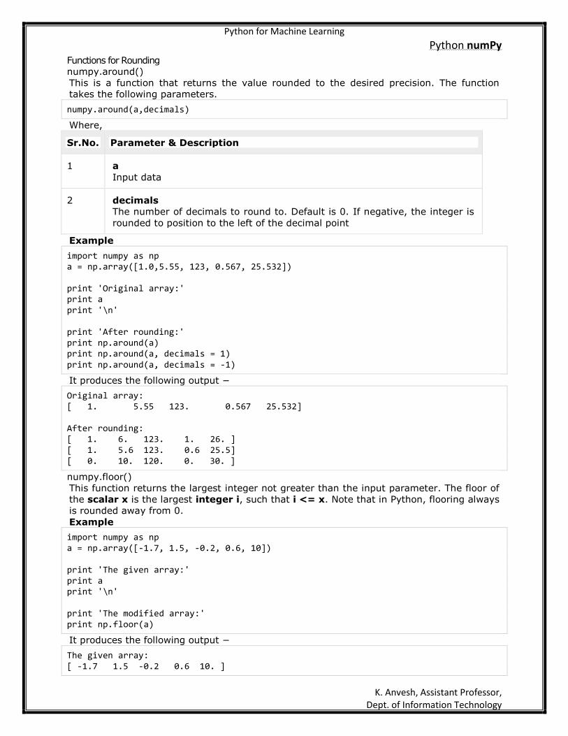
Functions for Rounding
numpy.around()
This is a function that returns the value rounded to the desired precision. The function
takes the following parameters.
numpy.around(a,decimals)
Where,
Sr.No. Parameter & Description
1 a
Input data
2 decimals
The number of decimals to round to. Default is 0. If negative, the integer is
rounded to position to the left of the decimal point
Example
import numpy as np a = np.array([1.0,5.55, 123, 0.567, 25.532]) print 'Original array:' print a print '\n' print 'After rounding:' print np.around(a) print np.around(a, decimals = 1) print np.around(a, decimals = -1)
It produces the following output −
Original array: [ 1. 5.55 123. 0.567 25.532] After rounding: [ 1. 6. 123. 1. 26. ] [ 1. 5.6 123. 0.6 25.5] [ 0. 10. 120. 0. 30. ]
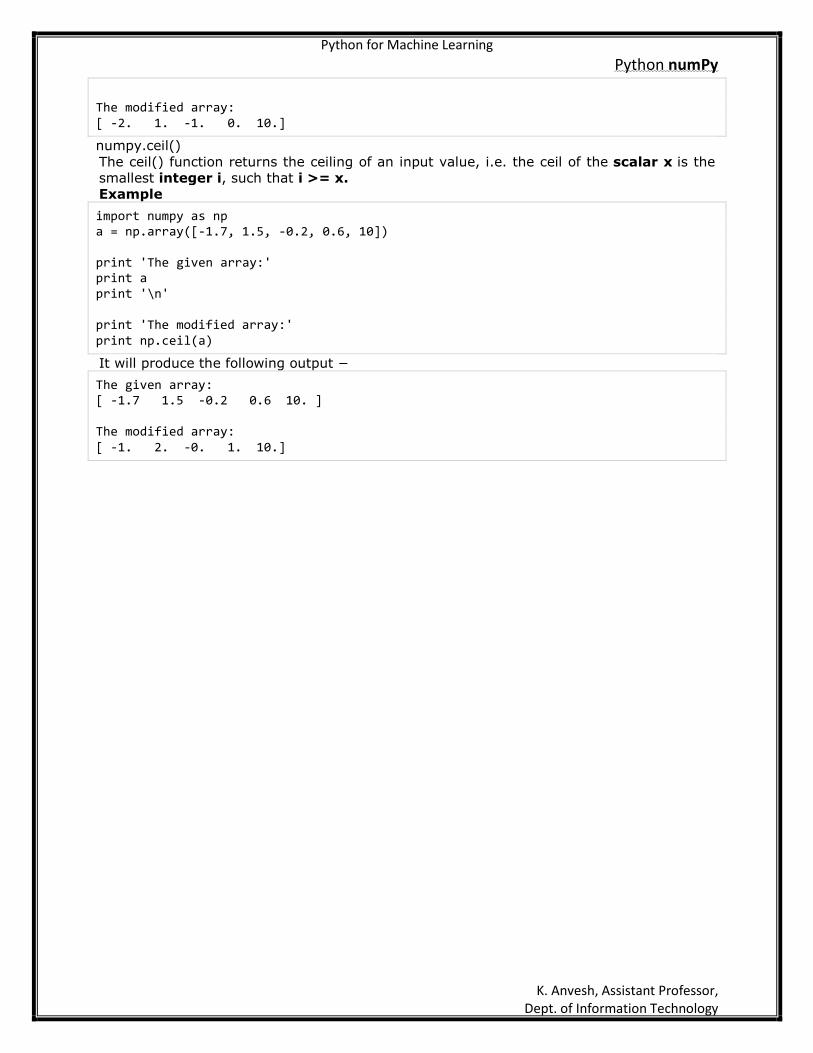
numpy.floor()
This function returns the largest integer not greater than the input parameter. The floor of
the scalar x is the largest integer i, such that i <= x. Note that in Python, flooring always
is rounded away from 0.
Example
import numpy as np a = np.array([-1.7, 1.5, -0.2, 0.6, 10]) print 'The given array:' print a print '\n' print 'The modified array:' print np.floor(a)
It produces the following output −
The given array: [ -1.7 1.5 -0.2 0.6 10. ]
Python for Machine Learning
Python numPy
K. Anvesh, Assistant Professor, Dept. of Information Technology
The modified array: [ -2. 1. -1. 0. 10.]
numpy.ceil()
The ceil() function returns the ceiling of an input value, i.e. the ceil of the scalar x is the
smallest integer i, such that i >= x.
Example
import numpy as np a = np.array([-1.7, 1.5, -0.2, 0.6, 10]) print 'The given array:' print a print '\n' print 'The modified array:' print np.ceil(a)
It will produce the following output −
The given array: [ -1.7 1.5 -0.2 0.6 10. ] The modified array: [ -1. 2. -0. 1. 10.]