Embed Size (px)
Citation preview

Numerics and the Conley Index: GAIO,
CHomP, and two examples
Sarah Day
Vrije Universiteit and Cornell University
Joint work with: K. Mischaikow and O. Junge
http://www.math.gatech.edu/~sday/thesis.pdf
(and references therein)
1

Computational considerations
1. high (or infinite) dimensional, continuous spaces do not fiteasily into a computer
2. sensitive dependence causes errors to blow-up in time
3. interpretation
2

Numerics and the Conley index
Three properties make the Conley index particularly well-suited
for numerical studies:
1. may tolerate a priori bounded error
2. computable in low dimensions (GAIO, CHomP)
3. provides rigorous information about the existence and struc-
ture of invariant sets
3

Goal: Develop computational techniques based on the Conleyindex to rigorously prove results about the structure of specificnonlinear dynamical systems.
The Method
1. Reduce the system to one which is computationally - friendly.(Galerkin projection, regularity, discretization)
2. Extract rigorous information from numerical computations onfinite dimensional systems. (GAIO, CHomP, Conley Index)
3. (For high dimensional systems) lift the results of the finitedimensional computations to the full, original system. (ConleyIndex, continuity, compactness)
balance computational costs with numerical precision
4

Two examples
1. Henon map
• simplified model of (chaotic) weather patterns
• 2-dimensional
• periodic orbits, connecting orbits, chaotic symbolic dy-
namics
• an example where simulation is misleading
2. Kot-Schaffer model
• models populations with discrete growth/dispersal phases
• infinite-dimensional
• chaotic symbolic dynamics
5
Computation: GAIO and CHomP
Two software packages for treating discrete dynamical systemsusing cubical structures:
• GAIO
– set-oriented numerical investigation of dynamical systems
– attractors and invariant manifolds, invariant measures, ...
– http://math-www.uni-paderborn.de/~agdellnitz/gaio/
• CHomP
– algorithmic homology computations
– cubical structures
– http://www.math.gatech.edu/~chom/
6

Discretizing space (GAIO)
Partition phase space W =∏m−1k=0 [x−k , x
+k ] into a finite number of
boxes by iteratively bisecting W with respect to the j-th coordi-
nate direction, j = 0,1, . . ..
The number of boxes grows exponentially in the dimension m of
W .
Instead, keep only a box covering of the maximal invariant set
(numerical effort essentially determined by dimension of the max-
imal invariant set).
7

Discretizing space (GAIO)
The boxes may be efficiently stored in a binary tree
• a coordinate direction is assigned to each level of the tree
• the root (depth = 0) corresponds to the box W
• all nodes at a depth k correspond to a subset Bk of a cubical
grid on W
8

Finite representation of the map (GAIO)
In a natural way, the (multivalued) map F on W defines a mul-tivalued map F on Bk: For B ∈ Bk, let
F(B) = {B ∈ Bk|F (B) ∩ B 6= ∅}
x
f(x)error
F(x)
“linear term + Lipschitz estimate”
The image may also be enlarged to in-
corporate additional error bounds.
F is stored as a (sparse) matrix or a graph, called the transitionmatrix, MF , or transition graph, GF .
9

Find interesting structures in MF (or GF) using graph theoretictechniques:
• k-periodic points of F are identified by nonzero diagonal en-tries of Mk
F
• more generally, recurrent sets of F are given by stronglyconnected components of GF
• in this graph, connecting orbits of F can be identified byshortest path algorithms (e.g. Dijkstra’s algorithm);
• compute the maximal invariant set of F (Szymzcak).
10

“Growing” isolating neighborhoods
Let S be a guess for an invariant set of F.
Algorithm (Growing Isolating Neighborhood)S = make isolated(S)
S := Inv(S,F)while o(S) 6⊂ S
S := S ∪ o(S)S := Inv(S,F)
if S ⊂ int |o(S)| return Selse return ∅
(o(S) denotes the one box neighborhood of S)
This algorithm returns a combinatorial isolated invariant set Sfor F with combinatorial isolating neighborhood I := o(S). Inthe case where |S| touches the boundary of W , the empty set isreturned.
11

Constructing index pairs (Szymczak)
Given an isolated invariant set S, let
N1 := S ∪ F(S)
and
N0 := N1 \ S
Then, |N | = (|N1|, |N0|) is an index pair for any continuous se-
lector f of F (and of |F|).12

Modification
There are two considerations which prompt us to modify thisconstruction.
1. The index pairs constructed in this way may be too large(especially for sets with high dimensional, strongly unstablebehavior).
2. Computation of the index map on this pair could introduce“folding effects”. Computation of the index map involvescomputing an auxiliary (or image) pair which contains theimage of the original index pair. The inclusion of the in-dex pair into the image pair must induce an isomorphism inrelative homology for the computed index map to be well-defined. This fails when the image of a box in N0 folds backto intersect to o(S) \ N1.
13

Modified index pairs
The following algorithm produces smaller index pairs (restrictedto a one-box neighborhood of S as motivated by Szymczak’sdefinition of a weak index pair) which also prohibit the wrappingeffect.
Algorithm (Modified Combinatorial Index Pair)
[P1,P0] = build ip(S)P0 := ∅E := (F(S) ∩ o(S)) \ Swhile E 6= ∅
P0 := P0 ∪ EE := (F(P0) ∩ o(S)) \ P0
P1 := S ∪ P0return [P1,P0]
14

Weak index pairs
Recall: A pair N = (N1, N0) of compact sets is a weak index
pair for f : Y → Y if and only if Inv(I, F ) ⊂ int(I) where I :=
cl(N1\N0) and the index map fN : (N1/N0, [N0]) → (N1/N0, [N0])
given by
fN([x]) =
{[f(x)] if x, f(x) ∈ N1 \N0[N0] otherwise
(1)
is a continuous map.
This weaker version is sufficient for defining the index.
15

Auxiliary pair
Define the auxiliary pair [Q1,Q0] by
Q1 := F(P1) and Q0 := Q1 \ S
Note that by construction, [P1,P0] = [Q1 ∩ o(S),Q0 ∩ o(S)].
Equivalently,
(|P1|, |P0|) = (|Q1| −A, |Q0| −A)
where A = |Q1 − o(S)| ⊂ |Q0|. By excision, the inclusion map
i : (|P1|, |P0|) ↪→ (|Q1|, |Q0|) induces an isomorphism i∗ in relative
homology. This property ensures that we prevent the folding
effect and, therefore, may compute a well-defined index map.
16

Computing the index, CHomP
By construction, F : [P1,P0] → [Q1,Q0] respects this pair struc-
ture, i.e. F(P1) ⊂ Q1 and F(P0) ⊂ Q0.
For i = 0,1, let Fi be |F| restricted to |Pi|.
Let ΓFi, be the graph of Fi : |Pi| → |Qi|. By construction of
F, the natural projection p : (ΓF1,ΓF0
) → (|P1|, |P0|) induces an
isomorphism in homology.
Then the map f∗ : H∗(|P1|, |P0|) → H∗(|P1|, |P0|) induced by any
continuous selector f of F in homology is f∗ = q∗ ◦ (p∗)−1 where
q is the natural projection (ΓF1,ΓF0
) → (|Q1|, |Q0|).
17

Efficient algorithms for cubical graph reductions which preserve
homology, in addition to other computational techniques, are
also used during this procedure.
Finally, if the inclusion map i : (|P1|, |P0|) ↪→ (|Q1|, |Q0|) induces
an isomorphism in homology then the index map is
fP∗ = (i∗)−1 ◦ f∗
This additional property that the inclusion map induces an iso-
morphism may be verified independently when working with a
general combinatorial index pair [P1,P0]. Alternatively, this prop-
erty is ensured by the construction of the modified combinatorial
index pair.

Using the indexThe Lefschetz number on the pointed space (P1/P0, [P0]) is
Λ(I, f) :=∞∑n=0
(−1)ntrfP,n
where I = P1 \ P0.
Theorem. If Λ(I, f) 6= 0, then f has a fixed point in I.
Proof. (Szymzcak) The point [P0] is a strong sink/isolated fixedpoint with index 1. The fixed point index of the set of all fixedpoints is Λ(I, f) + 1. If this total index is not equal to the indexof [P0], then there is a fixed point in I (different from [P0]).
Similarly,1. if Λ(I, fk) 6= 0, then f has a periodic orbit of period k
2. if Λ(I, fCn ◦ . . .◦fC1) 6= 0, then f has a periodic orbit traveling
through components C1, . . . , Cn
18

Example 1: the Henon map
h : R2 → R2
(xy
)→(
1− ax2 + y/55bx
)
With parameter values a = 1.3 and b = 0.2.
19
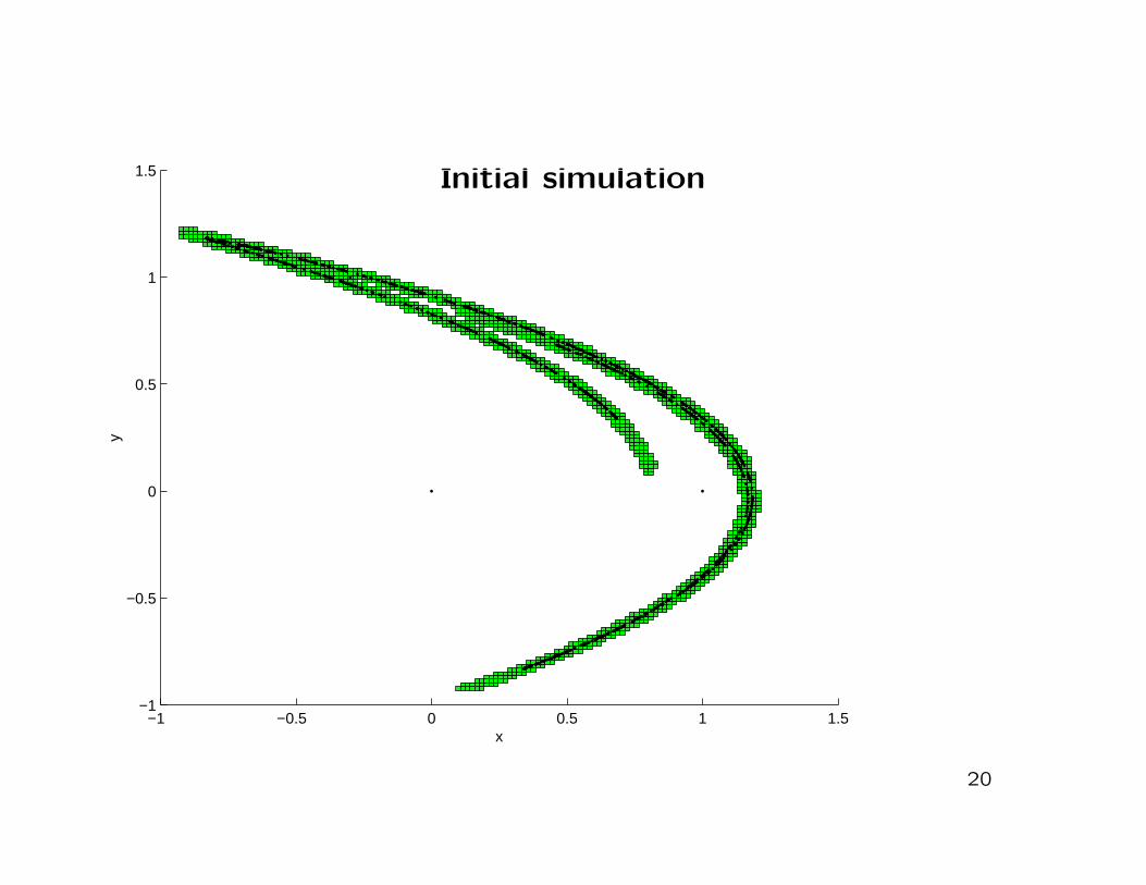
Initial simulation
−1 −0.5 0 0.5 1 1.5−1
−0.5
0
0.5
1
1.5
x
y
20

Finite representation
From these simulations, we choose a box to initialize a tree in
GAIO.
For our computations we choose to initially subdivide each box
14 times (subdividing 7 times in each of the two directions).
This results in 1188 boxes, each of box radius [0.0087,0.0087]
covering the maximal invariant set and a transition matrix, MH,
on these boxes.
21

Period 2 orbit
• Initial guess: nonzero entries of the diagonal of M2H (boxes
553 and 78)
• “grow” this initial two box collection into a combinatorial
isolated invariant set S for H
• construct the corresponding modified combinatorial index
pair, [P1,P2]
22

Modified index pair, period 2 orbit
−0.6 −0.4 −0.2 0 0.2 0.4 0.6 0.8 1 1.2−0.6
−0.4
−0.2
0
0.2
0.4
0.6
0.8
1
1.2
x
y
23

Period 2 orbit, index
Compute the index
• construct auxiliary pair [Q1,Q2]
• use CHomP, with [P1,P2], [Q1,Q2], and MH on P1
H∗(|P1|, |P0|) ∼= (0, Z2, 0, 0, . . .).
For an appropriate choice of basis,
hP,1 :=
[0 1−1 0
].
Each generator of H1(|P1|, |P0|) lies in a distinct connected com-ponent of |P1| \ |P0|.
24

Period 2 orbit, proof
Theorem. There exists a periodic orbit of minimal period two for
the Henon map with elements in each of the distinct connected
components of S.
Proof. The Lefschetz number Λ(I, h2) = −tr(h2P,1) = −2 is
nonzero so S contains a periodic point of period two. Further-
more, this orbit has minimal period two since the transition graph
on the two connected components of S prohibits there being a
fixed point.
25

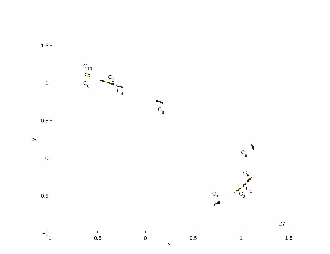
A connecting orbit
Initial guess: an orbit connecting a period 2 orbit to a period 4
orbit in MH at depth 16
Grow isolating neighborhood, construct modified index pair.
26
−1 −0.5 0 0.5 1 1.5−1
−0.5
0
0.5
1
1.5
C1
C2
C3
C4
C5
C6
C7
C8
C9
C10
x
y
27

H∗(|P1|, |P0|) ∼= (0, Z10, 0, 0, . . .).
hP,1 :=
0 −1 0 0 0 0 0 0 0 01 0 0 0 0 0 0 0 0 00 1 0 0 0 0 0 0 0 00 0 −1 0 0 0 0 0 0 00 0 0 1 0 0 0 0 0 00 0 0 0 −1 0 0 0 0 00 0 0 0 0 1 0 0 0 10 0 0 0 0 0 −1 0 0 00 0 0 0 0 0 0 −1 0 00 0 0 0 0 0 0 0 −1 0
.
Each of the 10 generators lies in a distinct component.
28

Connecting orbit, proof
Theorem. There exists an orbit for the Henon map which limitsin forwards time to a box neighborhood of a period 4 orbit, andin backwards time to a box neighborhood containing a period 2orbit.
Proof. The periodic orbits exist:
tr h2C1∪C2,1
= −2 and tr h4C7∪...∪C10,1
= −4.
hP∗ is not shift equivalent to hC1∪C2∗ ⊕ h∪i∈{7,8,9,10}Ci∗, so theConley indices of Inv(|S|, h) and Inv(∪i∈{1,2,7,8,9,10}Ci, h) are dif-ferent. Hence Inv(|S|, h) 6= Inv(∪i∈{1,2,7,8,9,10}Ci, h)
This, in addition to the transition information given by MH, com-pletes the proof.
29

Chaotic symbolic dynamics, 1d-unstable
Initial guess: a period four orbit, a period two orbit, and two
connecting orbits in the transition graph given by MH at depth
16
Grow isolating neighborhood, construct modified index pair.
30

−0.8 −0.6 −0.4 −0.2 0 0.2 0.4 0.6 0.8 1 1.2−0.8
−0.6
−0.4
−0.2
0
0.2
0.4
0.6
0.8
1
1.2
x
y
A
B
C
D
E
F
G
H
I
J
K
L
M
N
31

H∗(|P1|, |P0|) ∼= (0, Z15, 0, 0, . . .).
6
6
6
6
6
6
?
?
?
?
?
?
-�
�
-
�
-
ttttttt
tttttttA
N
M
L
K
J
I
B
C
D
E
F
G
H
1
6
6
6
6
6
6
?
?
?
?
?
?
-�
�
-
�
-
ttttttt
ttttttt
t
A
N
M
L
K
J
I
B
C
D
E1 E2
F
G
H
JJ
JJ
+
+
−
+
+
+
+
−
−
+ +
−
+
+
−
+
+
−+
1
transition graph on components index map on generators
32

Theorem There is a set contained in |S|, on which h is semi-
conjugate to the symbol subshift given by the transition graph.
Proof.
ΣT ΣT
S S
-σ
-
f
?
ρ
?
ρ
ΣT = {(Zi)i|(Zi, Zi−1)an edge in T}
ρ(x) = {Zi|f i(x) ∈ Zi}
σ is left shift by one symbol
• Study e.g. Λ(I, h42JIHGhF . . . hD . . . hK). Since for each peri-
odic symbol sequence, the corresponding Lefschetz number
is nonzero, there exists at least one corresponding periodic
orbit in S.
• ρ is continuous and S is compact. Therefore, ρ maps onto
ΣT , the closure of periodic orbits.33

Transition graph vs the index
Initial guess: connecting orbit from a period two orbit to a fixed
point given by MH at depth 14
34

−1 −0.5 0 0.5 1 1.5−1
−0.5
0
0.5
1
1.5
x
y
B
A

The computed index isH∗(|P1|, |P0|) ∼= (0, Z9, 0, 0, . . .)
hP,1 :=
0 −1 0 0 0 0 0 0 01 0 0 0 0 0 0 0 00 1 0 0 0 0 0 0 00 0 −1 0 0 0 0 0 00 0 0 −1 0 0 0 0 00 0 0 0 0 0 0 0 00 0 0 0 0 1 0 0 00 0 0 0 0 0 1 0 00 0 0 0 0 0 0 1 −1
.
hP,1 folds the only generator in Component A (column 5) andmaps it trivially to the generator in Component B (row 6).
Subdividing S at depth 14 to a depth of 24, MH prohibits aconnecting orbit of this type.
35

In infinite dimensions
Outline:
1. Reduce the system to a finite-dimensional system for compu-
tation (Galerkin projection, regularity, discretization)
2. Extract rigorous information from numerical computations on
the finite-dimensional system. (GAIO, CHomP, Conley Index)
3. Lift the results of the finite dimensional computations to
the full, original system. (lifting set: Conley Index, continuity,
compactness)
36

Example 2: an infinite dimensional map
The Kot-Schaffer growth-dispersal model for plants:
Φ : L2((−π, π),R) → L2((−π, π),R)
ψ 7→ Φ(ψ)
Φ(ψ)(x) =∫ π−π
D(x, y)g[ψ](y)dy,
growth operator: g[ψ]= µψ (1− cψ), where c−1 gives the localcarrying capacity, and µ > 0 is the (birth - death) rate.
dispersal kernel: D(x, y)= Σkbk exp(ik|x− y|), e.g. bk = 2−k
37
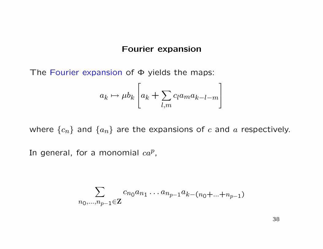
Fourier expansion
The Fourier expansion of Φ yields the maps:
ak 7→ µbk
ak +∑l,m
clamak−l−m
where {cn} and {an} are the expansions of c and a respectively.
In general, for a monomial cap,
∑n0,...,np−1∈Z
cn0an1 . . . anp−1ak−(n0+...+np−1)
38

Regularity
For the Kot-Schaffer system,
| < Φ[a], φk > | =∣∣∣ 12π
∫ π−π
∫ π−π
bkφk(x)g[a](x)dxdy∣∣∣
= |bk|∣∣∣∫ π−π
φk(x)g[a](x)dx∣∣∣
≤ |bk|‖φk‖‖g[a]‖≤ Cg,a|bk|
In particular, if |bk| ≤ Bbk
for some constants B > 0, b > 1, thenfor sufficiently large k,
| < Φ[a], φk > | ≤A
bk
where A = Cg,aB.
39

Restricted domain
We will study the maps on subsets of the form
Z =∏k
[a−k , a+k ]
where for some constants m,M > 0,
0 1 Mm-1
m M-1 k
variables explicit bounds asymptotic bounds Assk
40

Choosing an appropriate M
Projections onto modes 5 and 11 (order 10−4), and modes 50
and 51 (order 10−61). M = 50, [a−k , a+k ] =
[−12k, 12k
]for k ≥M
41

Error
a′k = f(m)k (a0, . . . , am−1) + f
(m+)k (a)
Suppose exponential decay, |ak| ≤ Ask
Lemma 1. If cn ∈ cn := Csn[−1,1], then
∑n0,n1,...,np−1∈Z
cn0an1 . . . anp−1ak−(n0+...+np−1)
⊆αpApC
sk
(b
β
)k[−1,1]
where 1 < bβ < s and α ≥ 2
ln s + bβ ln b
β
(e.g. bβ = 2s
s+1)
42

Choosing an appropriate m
m 3 4 5 6
ε(m+)k
0.02260.00220.0022
0.01920.00180.00050.0090
0.00590.00090.00020.00060.0023
0.00150.00020.00010.00030.00010.0006
1
Errors induced by neglecting the higher order modes for
different projection dimensions. m = 6
43

Definition. A set Z = N × V is a lifting set if
1. N =∏∞j=0[x
−j , x
+j ] is an isolating neighborhood for the finite-
dimensional, mulitivalued system given by the map PmΦ(·, V )
2. V =∏∞j=m[x−j , x
+j ] and for each j ≥ m, either
(a) (contraction) πjΦ(Z) ⊂ (x−j , x+j ), or
(b) (expansion) πjΦ(x) /∈ [x−j , x+j ] for all x ∈ Z with xj = x±j
where Pm is a projection onto the first m modes and πj is a
projection onto the jth mode.
This set may be used to compute the index in the infinite-
dimensional space.
44

Chaotic symbolic dynamics for Kot-Schaffer
45

6
6
6
6
?
?
?
?
-�
���� A
AAU
ttttt
ttttt
t A
� �?
G
H
I
J
K
F
E
D
C
B
1
6
6
6
6
6
?
?
?
?
?
?
��
��
�
��
��
�������
�
ttttttt
ttttttt
tG1
G2
H
I
J
K
A3
A4
tttF2@
@@I
F1
F3
F4
E
D
C
B
A2
A1
� �?
�
��
-�
+
−
+
−
−
−
+
−
+
+
−
+
−
+
+
+
+
++
−
+
1
N = A ∪ . . . ∪K, H2(N1, N0) = Z18,
S = Inv(N1 \N0, f), f∗ = PmΦ∗46

Chaotic symbolic dynamics for Kot-Schaffer
Theorem. There is an invariant set given with precision 10−10,
which under Φ is semi-conjugate to the chaotic subshift dynamics
given by the transition graph shown below.
6
6
6
6
?
?
?
?
-�
���� A
AAU
ttttt
ttttt
t A� �
?
G
H
I
J
K
F
E
D
C
B
47

Proof.
1. Construct a lifting set Z, (GAIO in first 6 modes, analysis in
higher modes all using formulas similar to the one given in
Lemma 1)
2. A similar argument to the one used for the Henon map com-
pletes the proof.
48