Numerically exact path-integral simulation of nonequilibrium quantum transport and dissipation

Dvira SegalChemical Physics Theory Group, Department of Chemistry, University of Toronto, Toronto, Ontario, Canada M5S 3H6

Andrew J. MillisDepartment of Physics, Columbia University, 538 W 120th Street, New York, New York 10027, USA

David R. ReichmanDepartment of Chemistry, Columbia University, 3000 Broadway, New York, New York 10027, USA

�Received 30 August 2010; published 18 November 2010�

We develop an iterative, numerically exact approach for the treatment of nonequilibrium quantum transportand dissipation problems that avoids the real-time sign problem associated with standard Monte Carlo tech-niques. The method requires a well-defined decorrelation time of the nonlocal influence functional for properconvergence to the exact limit. Since finite decorrelation times may arise either from temperature or from avoltage drop at zero temperature, the approach is well suited for the description of the real-time dynamics ofsingle-molecule devices and quantum dots driven to a steady state via interaction with two or more electronleads. We numerically investigate two nontrivial models: the evolution of the nonequilibrium population of atwo-level system coupled to two electronic reservoirs, and quantum transport in the nonequilibrium Andersonmodel. For the latter case, two distinct formulations are described. Results are compared to those obtained byother techniques.

DOI: 10.1103/PhysRevB.82.205323 PACS number�s�: 05.60.Gg, 03.65.Yz, 72.10.Fk, 73.63.�b

I. INTRODUCTION

There are several ways in which a quantal entity mayexhibit nontrivial departures from equilibrium. First, a sys-tem may evolve toward equilibrium after application of atransient external pulse or from a nonequilibrium initial con-dition. Simple examples of such situations are now relativelywell understood.1,2 Related to these types of departures fromequilibrium, but less well understood, are more challengingcases of “quantum quenches,” whereby the sudden change ina control parameter induces dynamics that probe nontrivialaspects of strong correlation or quantum criticality.3 Also un-derdeveloped is our understanding of quantum mechanicalsystems driven to nonequilibrium steady states via couplingto two or more electronic reservoirs. Since this is the case ofdirect relevance for the study of transport through quantumdots and molecular electronic devices,4,5 the complete de-scription of this type of nonequilibrium behavior is of prac-tical as well as fundamental interest.

There are essentially two main theoretical frameworks forthe calculation of properties related to the approach to, andattainment of, nonequilibrium steady states of the types men-tioned above. The first is the standard real-time Schwinger-Keldysh technique.6 This approach has led to the exact for-mulation of steady-state properties �e.g., the current� in termsof Keldysh Green’s functions.7 A variety of direct perturba-tive and renormalization-group calculations have naturallyemerged from this starting point.8–10 In addition, real-timeMonte Carlo �MC� methods have been formulated on thebasis of the Schwinger-Keldysh approach.11–13 The MonteCarlo methods are exact in principle but may be severelylimited by numerical sign problems, depending on the for-mulation, system, and regime under investigation.

The second framework involves the use of Lippmann-Schwinger scattering states14 to construct the properties of

nonequilibrium quantum steady state. This approach has ledto several rigorous results for integrable models.15 In the lastfew years this viewpoint, combined with the notion of Her-shfield’s steady-state density operator,16 has inspired the for-mulation of new nonperturbative approaches as well as nu-merical methods.17–20 Most recently, promising numericalrenormalization-group approaches have been put forwardbased directly on the construction of scattering states,21 andan extension to the density-matrix renormalization-groupmethod, incorporating real-time evolution, has beenpresented.22,23

Consideration of more standard classes of nonequilibriumrelaxation in dissipative systems such as the spin-bosonmodel has led to a variety of path-integral techniques for thenumerically exact propagation of the reduced density matrixof a small system coupled to its environment.1 These meth-ods, which include real-time Monte Carlo techniques11 aswell as deterministic iterative approaches,24–26 are connectedto the Schwinger-Keldysh-type framework discussed above.Here, as in the Schwinger-Keldysh technique, the approachto equilibrium along a particular time contour from a pre-scribed nonequilibrium initial condition is described. Ofthese approaches, iterative path-integral methods have hadparticular success.24 Such methods are based on the notionthat a well-defined bath correlation time �if one exists� ren-ders the range of the influence functional �IF� finite, allowingfor a controlled truncation of memory effects and thus a de-terministic propagation of observables that is free of the real-time sign problem.

While iterative path-integral approaches have been provensuccessful in describing nonequilibrium dynamics in simplespin-boson type models in the last 15 years, only recentlythey have been formulated and used in cases of relevance totransport through quantum dots and molecular electronic

PHYSICAL REVIEW B 82, 205323 �2010�

1098-0121/2010/82�20�/205323�13� ©2010 The American Physical Society205323-1

devices.27 In such systems, given that a chemical potentialdifference between electronic reservoirs leads to a well de-fined decorrelation time for dynamics even at zero tempera-ture, a memory time, beyond which correlations can bedropped, exists. This finite-memory characteristic allows thedevelopment of iterative techniques, capable of describingrelaxation in a wide and nontrivial region of parameterspace.

In this work we develop and apply a new iterative path-integral technique to two models of nonequilibrium transportand dissipation: the spin-fermion �SF� model and the single-impurity Anderson model �SIAM�. The techniques devel-oped here hold the potential for the exact description of long-time dynamics in systems driven to a nonequilibrium steadystate via coupling to two or more electronic reservoirs. Themethod we describe in this work is conceptually similar tothe iterative summation of real-time path integrals �ISPI� ap-proach of Thorwart and co-workers.27 The distinction be-tween these two approaches lies mainly in the propagationscheme and the manner in which the leads are traced out ofthe problem. In the iterative approach developed here, thereservoirs are represented as discrete levels and are elimi-nated numerically via the Blankenbecler-Scalapino-Sugar�BSS� identity.28 While this approach has the disadvantagethat an additional source of systematic error is introduceddue to the discretization of the lead degrees of freedom, wefind empirically that the error is easily controlled withoutundue computational expense. The advantage of this ap-proach is that the study of general models �for example, mul-tisite Hubbard “dots”� may be performed with essentially noreformulation of methodology. Taking advantage of this fact,we present a first set of exact results for the out-of-equilibrium two-lead spin-fermion model. A second differ-ence between the ISPI approach and the approach outlined inthis work is related to the propagation scheme. Here we com-bine our matrix formulation with a propagation scheme simi-lar to that described in Ref. 26. This allows for very efficientpropagation that may be trivially parallelized with commer-cially available software.29 These distinctions in scaling andflexibility of approach render our formulation as a usefulcompliment to the previously developed ISPI method.

This paper is organized as follows. Section II and Appen-dix A present some general aspects of the iterative propaga-tion technique. Section III contains a case study of the relax-ation of a tunneling system coupled to two electronicreservoirs. In Sec. IV we investigate nonequilibrium trans-port through an Anderson dot. In Sec. V we conclude. Ap-pendix B describes extensions to nonzero temperatures. Weinclude an alternative formulation of our approach for thenonequilibrium Anderson dot in Appendix C. This formula-tion may also hold promise in related path-integral ap-proaches such as the ISPI approach. Finally, Appendix Ddiscusses some aspects of the convergence analysis which isnecessary for elimination of the systematic errors in themethod.

II. GENERAL FORMULATION OF THEITERATIVE APPROACH

We consider a generic many-body system, consisting of afinite interacting region coupled to two infinite noninteract-

ing reservoirs. The Hamiltonian H can be partitioned into azeroth-order term H0 whose solution can be exactly obtained,typically containing few-body interactions, and a higher or-der interaction term H1. We introduce our iterative approachusing the reduced density matrix, �S=TrB���, obtained bytracing the total density matrix � over the reservoir degreesof freedom. The time evolution of �S�t� is exactly given by

�S�s�,s�;t� = TrB�s��e−iHt��0�eiHt�s�� . �1�

We decompose the evolution operator into a product of Nexponentials, eiHt= �eiH�t�N; �t= t /N, and define the discretetime evolution operator G�eiH�t. Different Trotter decompo-sitions can be employed for splitting this operator. For ex-ample, we find it convenient to approximate GeiH1�t/2eiH0�teiH1�t/2 when studying the spin-fermion model�Sec. III� while for the Anderson model �Sec. IV� we findthat it is useful to employ a decomposition of the form GeiH0�t/2eiH1�teiH0�t/2. The overall time evolution can be rep-resented in a path-integral formulation,

�S�s�,s�,t� = ds0+ ds1

+¯ dsN−1

+

� ds0− ds1

−¯ dsN−1

− TrB��s��G†�sN−1+ �

��sN−1+ �G†�sN−2

+ � ¯ �s0+���0��s0

−� ¯ �sN−2− �G�sN−1

− �

��sN−1− �G�s��� , �2�

where sk� are subsystem �or fictitious� degrees of freedom,

representing the discrete path on the forward �+� and back-ward �−� contours. As an initial condition we may assumethat ��0�=�B�S�0� with the bath �B� uncoupled to the sub-system. In what follows we refer to the integrand in Eq. �2�as an “Influence Functional,”30 and denote it byI�s0

� ,s1� , . . . ,sN

��, assigning sN+ =s�, sN

− =s�. Note that our defi-nition of the IF is more general than that contained in theoriginal work of Feynman and Vernon.30 We chose this loosedefinition to make connection with the iterative schemes de-veloped in the previous path-integral-based numericalwork.24

The IF combines the information of subsystem and bathdegrees of freedom with system-bath interactions, and itsform is analytically known only in special cases. For ex-ample, for a harmonic bath bilinearly coupled to a subsystemthe IF is an exponential of a quadratic form, multiplied byfree-subsystem propagation terms30

Ihar�s0�¯ sN

��

= exp�− �k=0

N

�k�=0

k

�sk+ − sk

−���k,k�sk�+ − �k,k�

� sk�− �

� �sN+ �e−iH0�t�sN−1

+ � ¯ �s0+��S�0��s0

−� ¯ �sN−1− �eiH0�t�sN

−� .

�3�

The coefficients �k,k� depend on the bath spectral functionand the temperature.24 For a general anharmonic environ-ment the IF may contain multiple-site interactions, where thecoefficients are not known in general.25 However, even when

SEGAL, MILLIS, AND REICHMAN PHYSICAL REVIEW B 82, 205323 �2010�

205323-2

the form of the IF is analytically known as in Eq. �3�, it stillcombines long-range interactions limiting brute force directnumerical simulations to very short times.

For a system coupled to a single thermal reservoir thischallenge has been tackled at finite temperatures where anatural bath decoherence time exists. As noted by Makri andMakarov,24 such cases are characterized by the useful featurethat nonlocal correlations contained in the IF decay exponen-tially, enabling a �controlled� truncation of the IF that in-cludes only a finite memory length. Based on this feature, aniterative scheme for evaluating the �finite-dimensional� pathintegral has been developed.24 While the original quasiadia-batic path-integral �QUAPI� algorithm was developed basedon the analytical pairwise form of the IF specific to harmonicreservoirs �Eq. �3��, a subsequent more general approach pro-posed in Ref. 26 is based only on the fact that memory ef-fects at finite temperatures generically vanish exponentiallyin the long-time limit.

This idea can be further employed to simulate the dynam-ics of a generic nonequilibrium bias-driven system.27 Sincein standard nonequilibrium situations bath correlations dieexponentially, the IF can be truncated beyond a memory time�c=Ns�t, corresponding to the time where beyond whichbath correlations may be controllably ignored. Here, Ns is aninteger, �t is the discretized time step, and �c is a correlationtime dictated by the nonequilibrium situation. For a systemunder a dc potential bias � at zero temperature, �c1 /�, while at temperatures for which T� tempera-ture sets the scale of the memory range. We therefore writethe total influence functional approximately as

I�s0�,s1

�,s2�, . . . ,sN

��

� I�s0�,s1

�, . . . ,sNs

� �Is�s1�,s2

�, . . . ,sNs+1� � ¯

�Is�sN−Ns

� ,sN−Ns+1� , . . . ,sN

�� �4�

with

Is�sk�,sk+1

� , . . . ,sk+Ns

� � =I�sk

�,sk+1� , . . . ,sk+Ns

� �

I�sk�,sk+1

� , . . . ,sk+Ns−1� �

. �5�

The errors in Eq. �4� are the usual Trotter error arising fromthe time discretization and the truncation to a finite memorytime �c=Ns�t. Both of these errors can be controlled. Equa-tion �4� can be understood as a simple generalization of thepairwise expression �3� for which

Ishar�sk

�,sk+1� , . . . ,sk+Ns

� � = f0�sk��f1�sk

�,sk+1� � ¯ fNs

�sk�,sk+Ns

� � .

�6�

The one-body and two-body functions f can be obtained byrearranging Eq. �3�. From these expressions we recursivelybuild the finite-range IF for a general model. We assume thatthe complete functional decays to zero with time constant�c=Ns�t, �Ns�N�, thus it can be approximated by the prod-uct

I�s0�,s1

�,s2�, . . . ,sN

��

� I�s0�,s1

�,s2�, . . . ,sN−1

� �I�s1

�,s2�,s3

�, . . . ,sN��

I�s1�,s2

�,s3�, . . . ,sN−1

� �. �7�

By recursively applying this rule, the truncated IF is furtherdecomposed until it correlates interactions within �c only,

I�s0�,s1

�,s2�, . . . ,sN

�� � I�s0�,s1

�, . . . ,sNs

� �

�I�s1

�,s2�, . . . ,sNs+1

� �

I�s1�,s2

�, . . . ,sNs

� �

I�s2�,s3

�, . . . ,sNs+2� �

I�s2�,s3

�, . . . ,sNs+1� �

¯

�I�sN−Ns

� ,sN−Ns+1� , . . . ,sN

��

I�sN−Ns

� ,sN−Ns+1� , . . . ,sN−1

� �, �8�

resulting in Eqs. �4� and �5�. The physical content of thisapproach, which is similar to that described in Ref. 26, isoutlined in Appendix A. The approach becomes exact as �c→�. Outside of the initial propagation step,Is�s0

� ,s1� , . . . ,sNs

� �� I�s0� ,s1

� , . . . ,sNs

� �, we can identify thefunctions Is �Eq. �4�� as the ratio between two IFs where thenumerator is calculated with an additional time step, Eq. �5�.Next, based on the decomposition �Eq. �4�� we can itera-tively integrate Eq. �2� by defining a multiple-time reduceddensity matrix �S�sk ,sk+1 , . . . ,sk+Ns−1�. Its initial value isgiven by �S�s0

� , . . . ,sNs−1� �= I, and it is evolution is dictated

by

�S�s1�, . . . ,sNs

� � = ds0��S�s0

�, . . . ,sNs−1� �Is�s0

�, . . . ,sNs

� �

�9�

with

Is�s0�, . . . ,sNs

� � = TrB��sNs

+ �G†�sNs−1+ � ¯ �s1

+�G†�s0+��s0

+���0��s0−�

��s0−�G�s1

−� ¯ �sNs−1− �G�sNs

− �� . �10�

A general propagation step involves integration over two�� � coordinates,

�S�sk+1� , . . . ,sk+Ns

� � = dsk��S�sk

�, . . . ,sk+Ns−1� �Is�sk

�, . . . ,sk+Ns

� � ,

�11�

where the time-local �tk=k�t� reduced density matrix is ob-tained by summing over all intermediate states,

�S�tk� = dsk−1�

¯ dsk−Ns+1� �S�sk−Ns+1

� , . . . ,sk�� . �12�

The evolution at shorter times k�Ns can be calculated in anumerically exact way. Before turning to specific models wewould like to make the following comments regarding theabove derivation. �i� The specific partitioning of the Hamil-tonian into H0 and H1 depends on the model investigated. Aswe show below, H0 may include only the subsystem degreesof freedom �spin-fermion model� or it may be constructedinvolving all two-body terms �Anderson model�. �ii� Obvi-ously, the decomposition �Eq. �7�� is not unique, however,

NUMERICALLY EXACT PATH-INTEGRAL SIMULATION OF… PHYSICAL REVIEW B 82, 205323 �2010�

205323-3

different schemes should lead to equivalent time evolution,and thus the partitioning is a matter of numerical conve-nience. �iii� The truncated IF �Is� is not necessarily a timeinvariant. As we show below, in the spin-fermion model Isdoes not depend on time, thus in this case it needs to beevaluated only once during the propagation scheme. In con-trast for the Anderson model standard use of the Hubbard-Stratonovich �HS� transformation leads to an IF expressionthat has to be updated at each time step. In Appendix C weoutline an approach that does not make use of the Hubbard-Stratonovich transformation and thus produces a form on theIF of the Anderson model that is time independent. �iv� Theshort-range function Is can be analytically evaluated in somespecial cases.24,25 For general reservoirs it may be evaluatednumerically, by using finite-size reservoirs as described inthe next section. �v� The approach outlined here is not re-stricted to specific statistics of the leads �boson or fermion�and is solely based on the fact that at finite temperatureand/or finite bias bath correlations exponentially decay atlong time. Therefore, it can be used to treat finite temperatureanharmonic bosonic environments26 as well as nonequilib-rium Fermi systems.

III. DISSIPATION IN THE NONEQUILIBRIUMSPIN-FERMION MODEL

A. Model

As a first example, we consider the dynamics of a two-state system coupled to two fermionic leads maintained atdifferent chemical potential values, the “Spin Fermionmodel.” This model has been considered in a series of recentpapers,31–34 and serves as a simple, albeit nontrivial, exampleexhibiting the generic behavior associated with the approachto a nonequilibrium steady state. In particular, at zero tem-perature the chemical-potential difference � sets the essen-tial energy scale for dephasing as is expected generically inmore complex models such as the nonequilibrium Kondomodel.35 It should be noted, however, the connection be-tween the model studied here and the nonequilibrium Kondomodel35 is more tenuous then that between the tunneling cen-ter model in equilibrium1 and the standard �equilibrium�Kondo model.36 We take as our Hamiltonian

HSF = H0 + H1,

H0 = HS, H1 = HB + HSB. �13�

The bath Hamiltonian HB is taken to be that of two indepen-dent leads � =L ,R� characterized by �spinless� free-fermionstatistics with different chemical potentials, namely,

HB = � ,k

�kc ,k† c ,k. �14�

The operator c ,k† �c ,k� creates �annihilates� an electron with

momentum k in the th lead. The system Hamiltonian HSconsists of a two-level system with a bare tunneling ampli-tude � and a level splitting B,

HS =B

2�z +

�

2�x. �15�

We take the general form for the system-bath coupling to be

HSB = � , �,k,k�

V ,k; �,k�c ,k† c �,k��z. �16�

Different versions of the model may be expressed via differ-ent forms of the coupling parameters V. In this paper wefocus on the model presented in Refs. 32 and 37, where themomentum dependence of the scattering potential is ne-glected. The system-bath scattering potentials are then givenby V , �, where , �=L ,R are the Fermi sea indices.

In the standard application of iterative path-integral ap-proaches, two features greatly simplify the propagation algo-rithm. First, the form of the Feynman-Vernon influence func-tional is known analytically. Second, the influence functionalis pairwise decomposable.24 As discussed in the previoussection, neither of these features is necessary for the numeri-cal implementation of an efficient iterative routine.

Recently, the analytical structure of the influence func-tional in the spin-fermion model considered here has beenelucidated, with a modified pairwise Coulomb gas behavioremerging at long times.33 However, our recent numerical re-sults have illustrated that in some cases for strong couplingof the system to the leads, most of the relevant dynamicalevolution occurs in time intervals before strict Coulomb gasbehavior holds.32

The exact dynamics follows Eq. �2�. Assuming separableinitial conditions ��t=0�=�S�t=0��B�t=0�, we can identifythe IF in the present model as

I�s0�,s1

�, . . . ,sN�� = �s0

+��S�0��s0−�

�K�sN�,sN−1

� � ¯ K�s2�,s1

��K�s1�,s0

��

� TrB�e−iH1�sN+ ��t/2e−iH1�sN−1

+ ��t¯

�e−iH1�s0+��t/2�B�0�eiH1�s0

−��t/2¯

�eiH1�sN−1− ��teiH1�sN

− ��t/2� . �17�

where H1=HB+HSB provides an adiabatic partitioningof the Hamiltonian, sk

� are forward �+� and backward �−�spin states along the paths, and K�sk+1

� ,sk��

= �sk+1+ �e−iHS�t�sk

+��sk−�eiHS�t�sk+1

− � is the propagator matrix forthe isolated subsystem.

The reduced density matrix is time propagated by em-ploying the iterative scheme �Eqs. �9�–�12��, where the func-tion Is �Eq. �5�� is calculated by taking ratios of the corre-sponding truncated IF �Eq. �17��. Note that this function istime-translationally invariant, thus we need to calculate itonly once.

B. Results

To numerically calculate the influence functional, we ex-press the lead Hamiltonians in terms of a finite number offermions. Then, as in the standard BSS Monte Carlo ap-proach to lattice fermions,28 the resulting trace may be ex-pressed as a simple determinant containing the one-body ma-

SEGAL, MILLIS, AND REICHMAN PHYSICAL REVIEW B 82, 205323 �2010�

205323-4

trices that represent exponentials of operators that arequadratic in fermionic creation and annihilation operators. Itshould be noted that this discretization of the bath leads tosystematic error in the results, unlike the case for the relatedISPI approach of Thorwart and co-workers.27 However, thediscretized approach for tracing out the bath is more flexiblein that cases where the analytic structure of the self-energyterms, such as structured “dot” with several correlated sites,may be easily treated. Furthermore, bosonic analogs of gen-eralized Anderson models may be treated easily as well,38

using the boson version of the BSS formalism.39 This factmay be of importance for the recently developed bosonicversions of dynamical mean field theory �DMFT�,40,41 wherefor out-of-equilibrium situations or at finite temperatures theapproach outlined here may potentially serve as a real-timeimpurity solver. Fortunately, since the time intervals overwhich the bath is “measured” are short, we have found thatthe infinite bath result is easy reached even with a relativelysmall number of effective bath fermions 40.

We use the following parameters: �=1, B=0, �0.5–2, and �V , �=��1−� , ��, considering only interbathsystem-bath couplings, where spin polarization is coupled toscattering events between the nonequilibrium reservoirs.Here � denotes the density of states of each Fermi sea. Forsimplicity we assume zero temperature. The generalization tofinite temperature is straightforward as outlined in AppendixB. Since the iterative approach outlined above requires afinite range of memory for the influence functional, we workwith a bias large enough to ensure facile convergence in thenumerical examples outlined below.

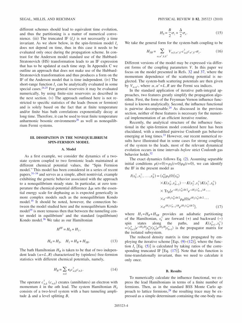
In Fig. 1 we show the dynamics of the spin polarization��z�t�� for several different values of the bias �, distributedsymmetrically between the L and R leads. The role of thechemical-potential difference as a temperature like contribu-tor to dephasing is clear.32 We analyze �inset� the memoryerror in our algorithm by increasing �c, keeping �t fixed. Asexpected, we find that �c roughly corresponds to 1 /�.Thus, for �1, taking �t=0.25, the dynamics is converg-

ing for Ns�5. A complete discussion of the appropriate con-vergence analysis is presented in Appendix D for the Ander-son model.

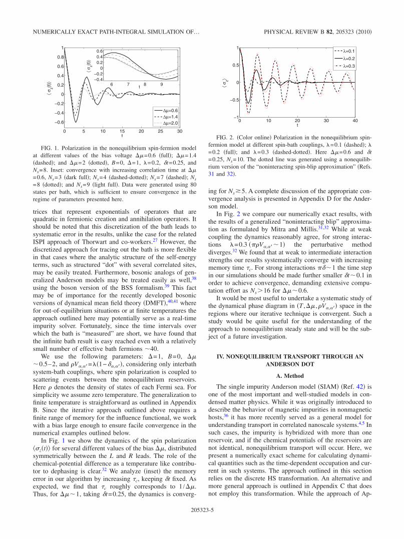
In Fig. 2 we compare our numerically exact results, withthe results of a generalized “noninteracting blip” approxima-tion as formulated by Mitra and Millis.31,32 While at weakcoupling the dynamics reasonably agree, for strong interac-tions �=0.3 ���V , �1� the perturbative methoddiverges.32 We found that at weak to intermediate interactionstrengths our results systematically converge with increasingmemory time �c. For strong interactions ��1 the time stepin our simulations should be made further smaller �t0.1 inorder to achieve convergence, demanding extensive compu-tation effort as Ns16 for �0.6.

It would be most useful to undertake a systematic study ofthe dynamical phase diagram in �T ,� ,�V , �� space in theregions where our iterative technique is convergent. Such astudy would be quite useful for the understanding of theapproach to nonequilibrium steady state and will be the sub-ject of a future investigation.

IV. NONEQUILIBRIUM TRANSPORT THROUGH ANANDERSON DOT

A. Method

The single impurity Anderson model �SIAM� �Ref. 42� isone of the most important and well-studied models in con-densed matter physics. While it was originally introduced todescribe the behavior of magnetic impurities in nonmagnetichosts,36 it has more recently served as a general model forunderstanding transport in correlated nanoscale systems.4,5 Insuch cases, the impurity is hybridized with more than onereservoir, and if the chemical potentials of the reservoirs arenot identical, nonequilibrium transport will occur. Here, wepresent a numerically exact scheme for calculating dynami-cal quantities such as the time-dependent occupation and cur-rent in such systems. The approach outlined in this sectionrelies on the discrete HS transformation. An alternative andmore general approach is outlined in Appendix C that doesnot employ this transformation. While the approach of Ap-

0 5 10 15 20 25 30

−0.6

−0.4

−0.2

0

0.2

0.4

0.6

0.8

1

t

⟨σz(t

)⟩

∆µ=0.6∆µ=1.4∆µ=2.0

6 7 8 9−0.4−0.2

00.20.40.6

t⟨σ

z(t)⟩

FIG. 1. Polarization in the nonequilibrium spin-fermion modelat different values of the bias voltage �=0.6 �full�; �=1.4�dashed�; and �=2 �dotted�, B=0, �=1, �=0.2, �t=0.25, andNs=8. Inset: convergence with increasing correlation time at �=0.6, Ns=3 �dark full�; Ns=4 �dashed-dotted�; Ns=7 �dashed�; Ns

=8 �dotted�; and Ns=9 �light full�. Data were generated using 80states per bath, which is sufficient to ensure convergence in theregime of parameters presented here.

0 10 20 30 40−1

−0.5

0

0.5

1

t

⟨σz⟩

λ=0.1

λ=0.2

λ=0.3

FIG. 2. �Color online� Polarization in the nonequilibrium spin-fermion model at different spin-bath couplings, �=0.1 �dashed�; �=0.2 �full�; and �=0.3 �dashed-dotted�. Here �=0.6 and �t=0.25, Ns=10. The dotted line was generated using a nonequilib-rium version of the “noninteracting spin-blip approximation” �Refs.31 and 32�.

NUMERICALLY EXACT PATH-INTEGRAL SIMULATION OF… PHYSICAL REVIEW B 82, 205323 �2010�

205323-5

pendix C offers several advantages, it is somewhat simpler toimplement the scheme described here, and for that reason wefollow it for the sake of illustrative calculation.

The SIAM model includes a resonant level of energy �d,described by the creation operator d�

† ��= ↑ ,↓ denotes thespin orientation� coupled to two fermionic leads � =L ,R� ofdifferent chemical potentials ,

HAM = ��

�dd�†d� + Ud↑

†d↑d↓†d↓ + �

,k,��kc ,k,�

† c ,k,�

+ � ,k,�

V ,kc ,k,�† d� + H.c. �18�

Here c ,k,�† �c ,k,�� denotes the creation �annihilation� of an

electron with momentum k and spin � in the lead, U standsfor the onsite repulsion energy, and V ,k are the impurity- lead coupling elements. Hamiltonian �18� can be also rewrit-ten as HAM =H0+H1, where H0 includes the exactly solvablenoninteracting part, and H1 includes the many-body term,

H0 = ��

�U/2 + �d�d�†d� + �

,k,��kc ,k,�

† c ,k,�

+ � ,k,�

V ,kc ,k,�† d� + H.c.,

H1 = U�nd,↑nd,↓ −1

2�nd,↑ + nd,↓� . �19�

Here nd,�=d�†d� is the impurity occupation number operator.

The shifted single-particle energies are denoted by Ed=�d+U /2. We also define �=� � , where � =��k�V ,k�2���−�k� is the hybridization energy of the resonant level withthe metal.

Our objective is to calculate the dynamics of a quadratic

operator A, either given by system or bath degrees of free-dom. This can be generally done by studying the Heisenberg

equation of motion of the exponential operator e�A with �here a variable that is taken to vanish at the end of the cal-culation,

�A�t�� = Tr��A� = lim�→0

�

��Tr���0�eiHAMte�Ae−iHAMt� . �20�

Here � is the total density matrix. For simplicity, we assumethat at the initial time �t=0� the dot and the bath are decou-pled, the impurity site is empty, and the bath is prepared in anonequilibrium �biased� zero-temperature state. The time

evolution of A can be obtained following a scheme analo-gous to that outlined in Sec. II for the reduced density ma-trix. For clarity, we rederive an explicit expression for thegeneralized IF in the present case as well.

First we use a standard factorization of the time evolutionoperator eiHAMt= �eiHAM�t�N, and assume the Trotter decompo-sition eiHAM�t��eiH0�t/2eiH1�teiH0�t/2�. The many body term H1is further eliminated by introducing auxiliary Ising variabless=� via the Hubbard-Stratonovich transformation,43

eiH1�t =1

2�s

e−s�+�nd,↑−nd,↓�,

e−iH1�t =1

2�s

e−s�−�nd,↑−nd,↓�, �21�

where ��=��� i��, ��=sinh−1�sin��tU /2��1/2, and ��=sin−1�sin��tU /2��1/2. The uniqueness of this transformationrequires U�t��. In what follows we use the following no-tation:

eH��s� � e−s���nd,↑−nd,↓�. �22�

Incorporating the Trotter decomposition and the HS transfor-mation �Eq. �22�� into Eq. �20�, we find that at zero tempera-

ture the time evolution of A is given by

�A�t�� = lim�→0

�

���0��eiH0�t/2eiH1�teiH0�t/2�Ne�A�e−iH0�t/2e−iH1�te−iH0�t/2�N�0�

= lim�→0

�

��� 1

22N ds1�ds2

�¯ dsN

��0��eiH0�t/2eH+�sN+ �eiH0�t/2� ¯ �eiH0�t/2eH+�s1

+�eiH0�t/2�e�A

� �e−iH0�t/2eH−�s1−�e−iH0�t/2� ¯ �e−iH0�t/2eH−�sN

− �e−iH0�t/2��0�� , �23�

SEGAL, MILLIS, AND REICHMAN PHYSICAL REVIEW B 82, 205323 �2010�

205323-6

where �0� is the initial �zero-temperature� state of the totalsystem. For convenience, we evaluate Eq. �23� by diagonal-izing the Hamiltonian H0 �see Eq. �19��, and rewriting H� interms of the new basis

H0 = ��

��b�†b�, H0 = VH0V−1,

H� = ��,��

������b�

†b�� �24�

with �� as the transformation matrix elements. We furthertransform both the operator of interest and the ground state

into the new representation A=VAV−1, �0�=V−1�0�. The IF isidentified as the integrand in Eq. �23�, where we truncateinteractions beyond the memory time �c=Ns�t,

I�sk�, . . . ,sk+Ns

� � =1

22Ns+2 �0�G+�sk+Ns

+ � ¯ G+�sk+�

�eiH0�k−1��te�A¯e−iH0�k−1��t

�G−�sk−� . . . G−�sk+Ns

− ��0� �25�

with G+�sk��= �eiH0�t/2eH+�sk

��eiH0�t/2� and G−=G+†. Finally, we

can build the function Is �Eq. �4�� using Eq. �5�, and the

operator of interest A may be propagated using a schemeanalogous to that developed for the reduced density matrix,Eqs. �9�–�12�.

Before presenting numerical results we make the follow-ing comments. First, in the present scheme the IF needs to beupdated at each time step since the truncated IF �Eq. �25��explicitly depends on the present time tk=k�t. Second, the

operator A can represent various quadratic operators. Thusquantities such as the impurity population or the currentthrough the junction12 may be investigated on the same foot-ing.

B. Results

The IF �Eq. �25�� is the core of our calculation. It is evalu-ated numerically using the zero-temperature relationship�0�eB�0�=det�eb�occ., where b is a single-particle operator, B=�b, and the determinant is carried over occupied statesonly. Extensions to finite temperature are standard, see Ap-pendix B. Similarly to the spin-fermion model we representthe reservoirs by a finite set of fermions, with energies de-termined by the metals’ dispersion relation. Calculationsmust be converged with respect to the number of discretelead states. The � derivative in Eq. �23� is handled numeri-cally, by calculating the IF for several �small� values of �.

In the following we typically use the following conven-tions and parameters: a symmetrically distributed voltagebias between two leads with �=0.4–0.6, a reservoir band-width of D=1, a resonant level energy Ed=0.3, and hybrid-ization strength � =0.025−0.1. Note that the actual hybrid-ization parameter utilized in the simulations is the couplingV ,k=�� /�� , where � is the density of states of the lead. For these parameters we find that convergence is

achieved using L�240 states per spin per bath. We have alsoverified that for �=0.4 the memory time �c3.2 leads toconvergence with �t=0.8 and Ns=4, provided U

� �3 �see Ap-pendix D�.

We begin by investigating the dynamics for a relativelysmall interaction U=0.1 ����L+�R and U /�=2�. In thisregime we are able to systematically converge the results ofour procedure with respect to the three sources of systematicerror, namely those associated with time step and bath dis-cretization as well as nonlocal memory truncation. Figure 3presents the time evolution of the dot occupation for twodifferent bias voltages, �=0.6 �dashed� and �=0.4 �full�,assuming the dot �Ed=0.3� is initially empty. The results arecompared to exact real-time MC simulations employing thehybridization expansion44 manifesting good agreement atthis relatively small U: at short times the IF data reproducethe MC features while close to steady state the MC resultsbecome increasingly unstable. The more recently developedweak-coupling expansion45 is capable of significantly ex-tending the time regime for which converged results may beobtained via Monte Carlo for symmetric cases, however thisrestriction limits the cases for which long-time results maybe obtained. The MC data presented in this paper were gen-erated at finite low temperature, 1 /T=200. We have verified�data not included� that for this temperature range the popu-lation dynamics essentially coincide with the strictly zero-temperature case. The extremely small deviations betweenMC data and our approach at U=0.1 in Fig. 3 are the resultof small differences in temperature and the fact that a sharp,finite band is assumed in our calculations.

Figure 4 presents the time evolution of �nd,�� with in-creasing on-site interaction. While we have not been able toovercome convergence issues for all times and all values ofU� , we find that dynamics are faithfully reproduced for all U

�at short times while accurate and converged results are cor-rectly obtainable only for U

� �3. The strict requirements forconvergence are presented in Appendix D. While this regime

0 5 10 15 20 25 300

0.05

0.1

0.15

0.2

0.25

0.3

t

⟨nd,

σ⟩

∆µ=0.6

∆µ=0.4

FIG. 3. �Color online� Resonant level dynamics at different val-ues of the voltage bias, �=0.6 �dashed� and �=0.4 �full�. U=0.1, � =0.025, Ed=0.3, and �c=3.2. The dotted lines show forreference the exact U=0 dynamics at �=0.6 and 0.4 �top to bot-tom�. The circles are the respective Monte Carlo points. Calcula-tions are performed at T=0 while Monte Carlo data utilizes T=1 /200 which is effectively converged to the T=0 limit.

NUMERICALLY EXACT PATH-INTEGRAL SIMULATION OF… PHYSICAL REVIEW B 82, 205323 �2010�

205323-7

is one where perturbation theory in U is accurate,45,46 webelieve that convergence restrictions are surmountable withinthe methodology presented in this work. Future study will bedevoted to this issue. Figure 5 compares the early propaga-tion obtained within the IF approach ��� to the MC data ���.Interestingly, while our approach does not capture the t2

characteristic at 0� t�3 due to the rough time discretiza-tion, the intermediate time dynamics is still correct. It shouldbe possible to devise an adaptive time propagation schemewhere the time step is increasing with time, keeping �c fixed.Future work will be devoted to improving convergence forlarge U and t. It is interesting to note that even though theresults at large time and on-site energy �U /��3� are notconverged and thus do not controllably represent a reliableestimate of population dynamics, the results are still reason-ably close to the MC data even for U

� =6.The effect of the impurity-bath hybridization strength has

been also analyzed. For � =0.025–0.1 and U=0.1–0.3 we

have obtained results in reasonable agreement with MC data,alike the behavior observed in Fig. 4. Furthermore, since ourmethod is nonperturbative in the hybridization strength, weexpect it to be useful for exploring the nonequilibriumKondo effect. However, the equilibrium Kondo physics can-not be probed within our treatment since at low temperaturesthe decorrelation time required for convergence becomes toolong for practical simulations.

Future work will be devoted for studying the time depen-dent and stationary current in the Anderson model. This canbe trivially implemented using Eq. �23� with the number op-

erator of the lead, A=�k,�c ,k,�† c ,k,�. The current at the

contact is then given by the time derivative I = ddt �A�. Ex-

tending the formalism to include nonzero-temperature effectsis a trivial task �Appendix B�. One could thus use ourmethod for studying the thermoelectric properties of �corre-lated� molecular systems, a topic of recent experimentalinterest.47 Note that contrary to wave function methods,48

convergence in our scheme is facilitated by going beyond thestrictly zero-temperature limit.

V. CONCLUSIONS

We have presented here a general path-integral-based it-erative scheme for studying the dissipative dynamics of bias-driven nonequilibrium systems. Our method relies on the fi-nite range of bath correlations in out-of-equilibrium cases,thus interactions within the influence functional may be trun-cated beyond a memory time dictated by the nonequilibriumconditions, and an iterative and deterministic scheme may bedeveloped. This scheme is in principle exact for cases whereconvergence with respect to truncation of memory effects isachieved.

The philosophy of our approach is similar to the previ-ously developed ISPI approach of Thorwart andco-workers.27 The distinction between the method presentedhere and ISPI is confined to the propagation scheme and thetechnique via which the leads are eliminated. The discretizedBSS-type approach28 to tracing out the reservoirs used heremay be employed in situations where the structure of thememory term is difficult to obtain analytically. Furthermore,the matrices involved in the iterative scheme are fixed insize, and this fact may present numerical advantages at verylong times. While our approach introduces an additionalsource of systematic error related to discretizing the leads,we have found that this error is easily controlled with limitednumerical cost. Thus, our approach presents a related butcomplimentary methodology to the ISPI technique. It shouldbe noted that currently the approach presented here and theISPI technique appear to have difficulty converging in simi-lar regions of parameter space that are accessible in somecases by, for example, the weak-coupling Monte Carloapproach.45 However approaches such as ISPI and the meth-odology presented allow for an accurate description of long-time dynamical features when they do converge, somethingthat is generically difficult with Monte Carlo schemes. In thisregard our approach is also complimentary to, and not com-petitive with, expansion based Monte Carlo schemes.44,45

0 5 10 15 20 25 300

0.05

0.1

0.15

0.2

0.25

0.3

0.35

t

⟨nd,

σ⟩U=0U=0.1U=0.3U=0.5

FIG. 4. �Color online� Population of the resonant level in theAnderson model. The results for U=0 �full�, U=0.1 �dashed�, U=0.3 �dashed-dotted�, and U=0.5 �dotted� are compared with theexact dynamics at U=0 ��� and Monte Carlo data �*, �, and ��.The physical parameters of the model are D=1, �=0.4, Ed=0.3,and � =0.025. The numerical parameters used are L=240 leadstates, �c=3.2 with Ns=4 and �t=0.8. Note that convergence andthus agreement with Monte Carlo cannot be achieved for t�10 ifU� �3.

0 1 2 3 4 5 60

0.05

0.1

0.15

t

<n d,

σ>

U=0.5

U=0.3

U=0.1

Influence Functional results: square

Monte−Carlo results: circle

FIG. 5. �Color online� Short time dynamics in the Andersonmodel ��� compared with Monte Carlo data ��� for U=0.5, 0.3,and 0.1 �top to bottom�. D=1, �=0.4, Ed=0.3, � =0.025, L=240, and �c=3.2 with Ns=4 and �t=0.8.

SEGAL, MILLIS, AND REICHMAN PHYSICAL REVIEW B 82, 205323 �2010�

205323-8

We have applied our technique to two prototype models:�i� the spin-fermion model of a spin coupled via a dipole-type interaction to two leads under a potential bias and �ii�the Anderson model, where a resonant level with an onsiterepulsion is coupled to nonequilibrium leads. In the first casethe dynamics of the tunneling system was investigated, re-covering damped oscillations for weak-intermediate cou-plings with the bias playing a role analogous to that of thetemperature in equilibrium systems. For the nonequilibriumAnderson model we focused our study on the resonant levelpopulation. Our method yields results in reasonable agree-ment with numerically exact Monte Carlo simulations forweak to intermediate onsite interactions U. For strong U de-viations are observed. The results presented in Appendix Dsuggest that the deviations are related to memory and time-step truncation errors which we have been unable to controlat the present time. Future work will be devoted to this issue.

Our path-integral formalism could be extended to handlebosonic degrees of freedom, representing, e.g., the nuclearcoordinates of the molecular bridge in the Anderson model�Anderson-Holstein model�. In particular, a phononic bath atthermal equilibrium could be easily incorporated, relying onthe analytic form of the Feynman-Vernon influencefunctional.30 Such a method, involving both fermionic andbosonic degrees of freedom, would become useful for ex-ploring vibrational effects in electron conduction. Othermodels, e.g., the multilevel Anderson model or a multisitechain, could be treated by adopting the formulation of Ap-pendix C. In summary, we expect this versatile numericallyexact approach to become useful in complementing existingtools, increasing our understanding of nonequilibrium quan-tum transport and dissipation characteristics in many bodymodels.

ACKNOWLEDGMENTS

D.S. acknowledges support from the Connaught grant.A.J.M. was supported by NSF under Grant No. DMR-0705847. D.R.R. would like to acknowledge the NSF forfinancial support. The authors acknowledge P. Werner forfruitful discussions and for providing the Monte Carlo dataand M. Thorwart for useful correspondence and encourage-ment.

APPENDIX A: JUSTIFICATION OF THETRUNCATION SCHEME

Here, we justify the breakup of the IF as prescribed byEq. �8�, demonstrating that the terms neglected account forinteractions beyond the memory range �c. Consider for sim-plicity the functional

I�s0�,s1

�,s2�,s3

�,s4�� � I�s0

�,s1�,s2

�,s3��

I�s1�,s2

�,s3�,s4

��I�s1

�,s2�,s3

��,

�A1�

truncated here by following Eq. �8� with Ns=3. Using a cu-mulant expansion for the total IF,25,26 we write the IF as aproduct of n-body interaction terms, I= I�2�� I�3�� I�4�

� I�5�, where each term is an exponent of a sum of then-body terms, For example, I�2�e−�i,jgi,j with pairwise in-teractions gi,j, I�3�e−�i,j,kgi,j,k, incorporating “three-body”interactions gi,j,k. Substituting this structure into Eq. �A1�, wefind that the following terms are not present on the right-hand side: The two- and three-body terms g0,4, g0,1,4, g0,2,4,and g0,3,4, four-body terms g0,1,2,4, g0,1,3,4, and g0,2,3,4, and afive-body element g0,1,2,3,4. These nonlocal interactions, con-necting spins beyond the memory range specified, Ns=3, areassumed to be small and are therefore discarded in our trun-cation scheme. Larger memory blocks, connecting more dis-tant time slices, may systematically be included until conver-gence with truncation of memory terms is reached.

To make this discussion concrete, consider a situationwhere nonequilibrium Coulomb gas behavior holds, as dis-cussed in Refs. 32 and 33. In such cases, the total influencefunctional will be of the form Iexp��ijC0��ti− tj���, whereC0�t����t� up to logarithmic corrections. Consider now Eq.�8�. Clearly the leading term contains all interactions be-tween “charges” separated by a distance in time that does notexceed �t0− tNs

�, namely, I�s0� ,s1

� , . . . ,sNs

� �

exp��ijNs � j=0

Ns−1C0��ti− tj���. Terms of the formI�s1

�,s2�,. . .,sNs+1

� �

I�s1�,s2

�,. . .,sNs� �

include only interactions between charges interacting overthe time intervals �tn− tNs+1�, where 0�n�Ns+1, withoutdouble counting terms already contained in I�s0

� ,s2� , . . . ,sNs

� �.This procedure is then iteratively continued until the com-plete influence functional is constructed. The error accruedoriginates from the neglect of terms in the exponent of theorder ��, where �= �ta− tb� and b−a�Ns+1. Thus, the pro-cedure is rendered controlled and is expected to converge tothe exact result as long as Ns is made large enough. It shouldbe noted that the approach outlined here is more general thanthis and is expected to hold at short times or very largecouplings where Coulomb gas behavior may break down, asdiscussed in Refs. 32 and 33.

APPENDIX B: EXTENSIONS OF THE IF TECHNIQUE TOFINITE TEMPERATURES

We present here the natural extension of our approach tofinite temperature. The core of our numerical calculation isthe IF, incorporating the Fermi sea degrees of freedom, e.g.,Eq. �17� for the spin-fermion model or Eq. �25� for theAnderson model. Assuming for simplicity a single Fermi sea,consider the following IF-like object:

Cf = TrB�eM1eM2�B� , �B1�

where M1 and M2 are quadratic operators and �B=e−�HB /TrB�e−�HB�, HB is the bath Hamiltonian, Eq. �14�.This correlation function can be expressed by single-particleoperators,49

Cf = det�I − f��� + em1em2f���� . �B2�

Here f���= �1+e���−��−1 is the Fermi-Dirac distributionfunction, � is the inverse temperature, I is the unit operator,and m1 and m2 are single-particle operators corresponding toM1 and M2, respectively. This expression can be trivially

NUMERICALLY EXACT PATH-INTEGRAL SIMULATION OF… PHYSICAL REVIEW B 82, 205323 �2010�

205323-9

extended to include more exponential terms,eM1eM2 , . . . ,eMN, as necessary for the evaluation of the IFexpression. For multiple-independent reservoirs, �B=�L � �R,the above relation can be generalized,

Cf = TrL TrR�eM1eM2�L � �R� = det���IL − fL���� � IR�

���IR − fR���� � IL� + em1em2�fL��� � IR��fR��� � IL�� .

�B3�

Here I is the identity matrix for the space; =L ,R, andf ���= �1+e� ��− ��−1. The above expressions reduce to theones used in the text for T=0.

APPENDIX C: AN ALTERNATIVE FORMULATION:NONEQUILIBRIUM TRANSPORT THROUGH

AN ANDERSON DOT

We present here an alternative formulation for calculatingthe dot properties in the SIAM without invoking theHubbard-Stratonovich transformation. This formulation isbased on a different Trotter decomposition than that used inSec. IV. While the resulting expressions are more complexfor the decomposition described here, it has the advantagethat the resulting IF need not be updated each time step.Furthermore, since fewer terms of the Hamiltonian are splitin the Trotter decomposition, it is possible that larger timesteps may be taken with the decomposition presented here.Further work investigating this approach, which is not con-fined to the Anderson model, will be presented in a futurework. We refer to the approach developed in Sec. IV asSIAM I, and to the method of this appendix as SIAM II.

We begin by partitioning Hamiltonian �18� as follows: H0includes the subsystem �dot� terms, and H1 includes the twononinteracting leads �HB� and system-bath couplings �HSB�

HAM = H0 + H1, H1 = HB + HSB,

H0 = ��

�dnd,� + Und,↑nd,↓,

HB = � ,k,�

�kc ,k,�† c ,k,�, HSB = �

,k,�V ,kc ,k,�

† d� + H.c.

�C1�

Here nd,�=d�†d� is the impurity number operator and c ,k,�

† isa creation operator of an electron at the lead with a spin �and momentum k. Note that H0 can be explicitly describedby a four-state system, �1�= �0,0�, �2�= �↑ ,0�, �3�= �↓ ,0�, and�4�= �↑ ,↓�, corresponding to an empty dot, a single occupieddot of �= ↑ ,↓, and a double occupancy state. When U isvery large �U→��, we effectively have a three-state systemsince double occupancy becomes negligible. The energies ofthese four subsystem states are E1=0, E2,3=�d, and E4=�d+U.

Consider the reduced density matrix �S=TrB��� obtainedby tracing the total density matrix � over the reservoir de-grees of freedom. The time evolution of �S�t� is exactlygiven by

�S�a,a�,t� = TrB�a�e−iHAMt��0�eiHAMt�a�� , �C2�

where �a� and �a�� are subsystem states, as described above.Using the standard Trotter breakup, eiHt= �eiH�t�N, �t= t /N,and eiHAM�t�eiH0�t/2eiH1�teiH0�t/2, we can rewrite Eq. �C2� in apath-integral formulation,

�S�a,a�,t� = ds0+ ds1

+¯ dsN−1

+ ds0− ds1

−¯ dsN−1

−

�TrB��a�e−iH0�t/2e−iH1�te−iH0�t/2�sN−1+ �

��sN−1+ �e−iH0�t/2e−iH1�te−iH0�t/2�sN−2

+ � ¯

��s0+���0��s0

−� ¯ �sN−2− �eiH0�t/2eiH1�teiH0�t/2�sN−1

− �

��sN−1− �eiH0�t/2eiH1�teiH0�t/2�a��� , �C3�

where sk are subsystem states. As an initial condition we mayassume that ��0�=�B�S�0� with the bath �B� uncoupled to thesubsystem. We focus next on the following matrix elementsin Eq. �C3�:

Ga,b��t� � �a�e−iH0�t/2e−iH1�te−iH0�t/2�b�

= e−i�Ea+Eb��t/2�a�e−iH1�t�b� . �C4�

To compute �a�e−iH1�t�b� note that it is advantageous to useagain the Trotter splitting

�a�e−iH1�t�b� � e−iHB�t/2�a�e−iHSB�t�b�e−iHB�t/2. �C5�

We thus focus next on the matrix element

Oa,b = �a�e−iHSB�t�b� , �C6�

a quadratic operator in the space of the noninteracting elec-trons. It is useful to define the “composite” fermion c0,�=� ,kV ,kc ,k,�, leading to HSB����c0,�

† d�+d�†c0,��. In this

representation a direct expansion of the exponential gives

e�HSB = I + �cosh � − 1�a2 + sinh �a1 �C7�

with �=−i�t, a1=HSB, and a2=���d�d�†c0,�

† c0,�d�d�† +H.c.�.

The operator �Eq. �C6�� is therefore of the form, Oa,b= +�c0,�+��c0,�

† +�c0,�† c0,�+��c0,�c0,�

† , with constant coeffi-cients ,� ,�. Substituting the pieces �Eqs. �C5�–�C7�� intoEq. �C4� yields

Ga,b��t� � e−i�Ea+Eb��t/2e−iHB�t/2Oa,be−iHB�t/2, �C8�

incorporating linear combinations of bath operators c0,� up toa quadratic order. Finally, we put all pieces together into Eq.�C3� and obtain the reduced dynamics

�S�a,a�,t� = ds0+¯ dsN−1

+ ds0−¯ dsN−1

− �s0+��S�0��s0

−�

�exp�− i�t�j=1

N−1

Esj+ + i�t�

j=1

N−1

Esj−

− i�Ea + Es0+��t/2 + i�Ea� + Es0

−��t/2�

� TrB��e−iHB�t/2Oa,sN−1+ e−iHB�tOsN−1

+ ,sN−2+

�e−iHB�t¯ Os1

+,s0+e−iHB�t/2��B�0��e−iHB�t/2

SEGAL, MILLIS, AND REICHMAN PHYSICAL REVIEW B 82, 205323 �2010�

205323-10

�Os0−,s1

−e−iHB�tOs1−,s2

−e−iHB�t¯ OsN−1

− ,a�e−iHB�t/2�� .

�C9�

Identifying the integrand as the IF, we can use the approachof Sec. II, define the truncated IF Is, and iteratively propagatethe reduced density matrix to long times.

The approach developed here �SIAM II� has three mainadvantages over the method described in the main text�SIAM I�, see Sec. IV. First, since the present method doesnot rely on the Hubbard-Stratonovich transformation it canbe applied to general many body interaction Hamiltonianswhile SIAM I is restricted to the Anderson model. Second,since the Trotter error in SIAM II is due to system-bathfactorization, rather than one-body-many-body splitting as inSIAM I, the method described here should be beneficial incalculating dynamics of weakly coupled system-bath modelswith arbitrarily large many body �local� interactions. Finally,this method also suggests a computational advantage over

SIAM I since the IF here �integrand of Eq. �C9�� is timeindependent, unlike the IF of Eq. �25� which needs to berecalculated at each time step.

APPENDIX D: CONVERGENCE ANALYSIS FOR THEANDERSON MODEL

There are three separate sources of systematic error withinour approach. �i� Bath discretization error. The electronicreservoirs are explicitly included in our simulations, and weuse bands extending from −D to D with a finite number ofstates per bath per spin �L�. This is in contrast to standardapproaches where a wideband limit is assumed and analyti-cal expressions for the reservoirs Green’s functions areadopted.12,27,44 �ii� Trotter error. The time discretization errororiginates from the approximate factorization of the totalHamiltonian into the noncommuting H0 �two-body� and H1�many-body� terms, see text after Eq. �20�. While for U→0 and for small time steps �t→0 the decomposition isexactly satisfied, for large U one should go to a sufficientlysmall time step in order to avoid significant error buildup.�iii� Memory error. Our approach assumes that bath correla-tions exponentially decay resulting from the nonequilibriumcondition ��0. Based on this crucial element, the influ-ence functional may be truncated to include only a finitenumber of fictitious spins Ns, where �c=Ns�t1 /�. Thetotal IF is retrieved by taking the limit Ns→N, �N= t /�t�.

These three errors can be systematically eliminated byincreasing the number of bath states, choosing a smallenough time step, and adopting a sufficiently long memorytime. Note however that the last two strategies are linked:increasing �c essentially means increasing the time step sincethe memory length is restricted to small values Ns=4–6 forpractical-computational reasons. Thus, as in standardQUAPI,24 one should find an optimal balance between thetime-step error and the memory size that correctly representsthe dynamics. Reference 50 suggests a systematic approachfor reaching convergence using the QUAPI method, elimi-nating the Trotter discretization error and the memory trun-cation inaccuracy by extrapolating the data to vanishing timestep and to infinite memory time.

0 5 10 15 20 25 300

0.05

0.1

0.15

0.2

0.25

0.3

0.35

0.4

t

⟨nd,

σ⟩

L= 20, 40, 80, 120, 240

↓

U=0.1

U=0.5

0 0.02 0.04 0.060

0.2

0.4

L−1<n d,

σ>

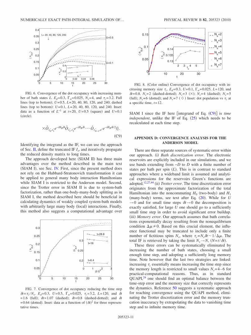
FIG. 6. Convergence of the dot occupancy with increasing num-ber of bath states L. Ed=0.3, � =0.025, Ns=4, and �c=3.2. Fulllines �top to bottom�; U=0.5, L=20, 40, 80, 120, and 240; dashedlines �top to bottom�: U=0.1, L=20, 40, 80, 120, and 240. Inset:data as a function of L−1 at t=20, U=0.5 �square� and U=0.1�circle�.

0 5 10 15 20 25 300

0.05

0.1

0.15

0.2

0.25

0.3

t

⟨nd,

σ⟩

0 1 2 3

0.2

0.25

0.3t=16

t=28.8

t=6.4

(δ t)2

⟨nd,

σ⟩

FIG. 7. Convergence of dot occupancy reducing the time step�t=�c /Ns. Ed=0.3, U=0.5, � =0.025, �c=3.2, L=120, and �t=1.6 �full�; �t=1.07 �dashed�; �t=0.8 �dashed-dotted�; and �t=0.64 �dotted�. Inset: data as a function of ��t�2 for three represen-tative times.

0 10 20 300

0.05

0.1

0.15

⟨nd,

σ⟩

t

2 3 4 5

0.13

0.135

0.14

⟨nd,

σ⟩

τc

Ns=2

Ns=3

Ns=4

Ns=5

Ns=6

Ns=7

FIG. 8. �Color online� Convergence of dot occupancy with in-creasing memory size �c. Ed=0.3, U=0.1, � =0.025, L=120, and�t=0.8. Ns=2 �dashed-dotted�; Ns=3 ���; Ns=4 �dashed�; Ns=5�full�; Ns=6 �dotted�; and Ns=7 �� � Inset: dot population vs �c ata specific time, t=12.

NUMERICALLY EXACT PATH-INTEGRAL SIMULATION OF… PHYSICAL REVIEW B 82, 205323 �2010�

205323-11

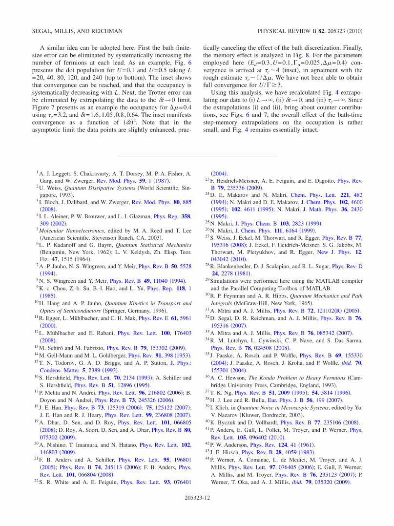
A similar idea can be adopted here. First the bath finite-size error can be eliminated by systematically increasing thenumber of fermions at each lead. As an example, Fig. 6presents the dot population for U=0.1 and U=0.5 taking L=20, 40, 80, 120, and 240 �top to bottom�. The inset showsthat convergence can be reached, and that the occupancy issystematically decreasing with L. Next, the Trotter error canbe eliminated by extrapolating the data to the �t→0 limit.Figure 7 presents as an example the occupancy for �=0.4using �c=3.2, and �t=1.6,1.05,0.8,0.64. The inset manifestsconvergence as a function of ��t�2. Note that in theasymptotic limit the data points are slightly enhanced, prac-

tically canceling the effect of the bath discretization. Finally,the memory effect is analyzed in Fig. 8. For the parametersemployed here �Ed=0.3,U=0.1,� =0.025,�=0.4� con-vergence is arrived at �c4 �inset�, in agreement with therough estimate �c1 /�. We have not been able to obtainfull convergence for U /��3.

Using this analysis, we have recalculated Fig. 4 extrapo-lating our data to �i� L→�, �ii� �t→0, and �iii� �c→�. Sincethe extrapolations �i� and �ii�, bring about counter contribu-tions, see Figs. 6 and 7, the overall effect of the bath-timestep-memory extrapolations on the occupation is rathersmall, and Fig. 4 remains essentially intact.

1 A. J. Leggett, S. Chakravarty, A. T. Dorsey, M. P. A. Fisher, A.Garg, and W. Zwerger, Rev. Mod. Phys. 59, 1 �1987�.

2 U. Weiss, Quantum Dissipative Systems �World Scientific, Sin-gapore, 1993�.

3 I. Bloch, J. Dalibard, and W. Zwerger, Rev. Mod. Phys. 80, 885�2008�.

4 I. L. Aleiner, P. W. Brouwer, and L. I. Glazman, Phys. Rep. 358,309 �2002�.

5 Molecular Nanoelectronics, edited by M. A. Reed and T. Lee�American Scientific, Stevenson Ranch, CA, 2003�.

6 L. P. Kadanoff and G. Baym, Quantum Statistical Mechanics�Benjamin, New York, 1962�; L. V. Keldysh, Zh. Eksp. Teor.Fiz. 47, 1515 �1964�.

7 A.-P. Jauho, N. S. Wingreen, and Y. Meir, Phys. Rev. B 50, 5528�1994�.

8 N. S. Wingreen and Y. Meir, Phys. Rev. B 49, 11040 �1994�.9 K.-c. Chou, Z.-b. Su, B.-l. Hao, and L. Yu, Phys. Rep. 118, 1

�1985�.10 H. Haug and A. P. Jauho, Quantum Kinetics in Transport and

Optics of Semiconductors �Springer, Germany, 1996�.11 R. Egger, L. Mühlbacher, and C. H. Mak, Phys. Rev. E 61, 5961

�2000�.12 L. Mühlbacher and E. Rabani, Phys. Rev. Lett. 100, 176403

�2008�.13 M. Schiró and M. Fabrizio, Phys. Rev. B 79, 153302 �2009�.14 M. Gell-Mann and M. L. Goldberger, Phys. Rev. 91, 398 �1953�.15 T. N. Todorov, G. A. D. Briggs, and A. P. Sutton, J. Phys.:

Condens. Matter 5, 2389 �1993�.16 S. Hershfield, Phys. Rev. Lett. 70, 2134 �1993�; A. Schiller and

S. Hershfield, Phys. Rev. B 51, 12896 �1995�.17 P. Mehta and N. Andrei, Phys. Rev. Lett. 96, 216802 �2006�; B.

Doyon and N. Andrei, Phys. Rev. B 73, 245326 �2006�.18 J. E. Han, Phys. Rev. B 73, 125319 �2006�; 75, 125122 �2007�;

J. E. Han and R. J. Heary, Phys. Rev. Lett. 99, 236808 �2007�.19 A. Dhar, D. Sen, and D. Roy, Phys. Rev. Lett. 101, 066805

�2008�; D. Roy, A. Soori, D. Sen, and A. Dhar, Phys. Rev. B 80,075302 �2009�.

20 A. Nishino, T. Imamura, and N. Hatano, Phys. Rev. Lett. 102,146803 �2009�.

21 F. B. Anders and A. Schiller, Phys. Rev. Lett. 95, 196801�2005�; Phys. Rev. B 74, 245113 �2006�; F. B. Anders, Phys.Rev. Lett. 101, 066804 �2008�.

22 S. R. White and A. E. Feiguin, Phys. Rev. Lett. 93, 076401

�2004�.23 F. Heidrich-Meisner, A. E. Feiguin, and E. Dagotto, Phys. Rev.

B 79, 235336 �2009�.24 D. E. Makarov and N. Makri, Chem. Phys. Lett. 221, 482

�1994�; N. Makri and D. E. Makarov, J. Chem. Phys. 102, 4600�1995�; 102, 4611 �1995�; N. Makri, J. Math. Phys. 36, 2430�1995�.

25 N. Makri, J. Phys. Chem. B 103, 2823 �1999�.26 N. Makri, J. Chem. Phys. 111, 6164 �1999�.27 S. Weiss, J. Eckel, M. Thorwart, and R. Egger, Phys. Rev. B 77,

195316 �2008�; J. Eckel, F. Heidrich-Meisner, S. G. Jakobs, M.Thorwart, M. Pletyukhov, and R. Egger, New J. Phys. 12,043042 �2010�.

28 R. Blankenbecler, D. J. Scalapino, and R. L. Sugar, Phys. Rev. D24, 2278 �1981�.

29 Simulations were performed here using the MATLAB compilerand the Parallel Computing Toolbox of MATLAB.

30 R. P. Feynman and A. R. Hibbs, Quantum Mechanics and PathIntegrals �McGraw-Hill, New York, 1965�.

31 A. Mitra and A. J. Millis, Phys. Rev. B 72, 121102�R� �2005�.32 D. Segal, D. R. Reichman, and A. J. Millis, Phys. Rev. B 76,

195316 �2007�.33 A. Mitra and A. J. Millis, Phys. Rev. B 76, 085342 �2007�.34 R. M. Lutchyn, L. Cywinski, C. P. Nave, and S. Das Sarma,

Phys. Rev. B 78, 024508 �2008�.35 J. Paaske, A. Rosch, and P. Wolfle, Phys. Rev. B 69, 155330

�2004�; J. Paaske, A. Rosch, J. Kroha, and P. Wolfle, ibid. 70,155301 �2004�.

36 A. C. Hewson, The Kondo Problem to Heavy Fermions �Cam-bridge University Press, Cambridge, England, 1993�.

37 T. K. Ng, Phys. Rev. B 51, 2009 �1995�; 54, 5814 �1996�.38 H. J. Lee and R. Bulla, Eur. Phys. J. B 56, 199 �2007�.39 I. Klich, in Quantum Noise in Mesoscopic Systems, edited by Yu.

V. Nazarov �Kluwer, Dordrecht, 2003�.40 K. Byczuk and D. Vollhardt, Phys. Rev. B 77, 235106 �2008�.41 P. Anders, E. Gull, L. Pollet, M. Troyer, and P. Werner, Phys.

Rev. Lett. 105, 096402 �2010�.42 P. W. Anderson, Phys. Rev. 124, 41 �1961�.43 J. E. Hirsch, Phys. Rev. B 28, 4059 �1983�.44 P. Werner, A. Comanac, L. de Medici, M. Troyer, and A. J.

Millis, Phys. Rev. Lett. 97, 076405 �2006�; E. Gull, P. Werner,A. Millis, and M. Troyer, Phys. Rev. B 76, 235123 �2007�; P.Werner, T. Oka, and A. J. Millis, ibid. 79, 035320 �2009�.

SEGAL, MILLIS, AND REICHMAN PHYSICAL REVIEW B 82, 205323 �2010�

205323-12

45 P. Werner, T. Oka, M. Eckstein, and A. J. Millis, Phys. Rev. B81, 035108 �2010�.

46 L. Muehlbacher, D. Urban, and A. Komnik, arXiv:1007.1793�unpublished�.

47 P. Reddy, S. Y. Jang, R. A. Segalman, and A. Majumdar, Science315, 1568 �2007�.

48 H. Wang and M. Thoss, J. Chem. Phys. 119, 1289 �2003�; 131,024114 �2009�.

49 D. A. Abanin and L. S. Levitov, Phys. Rev. Lett. 94, 186803�2005�.

50 J. Eckel, S. Weiss, and M. Thorwart, Eur. Phys. J. B 53, 91�2006�.

NUMERICALLY EXACT PATH-INTEGRAL SIMULATION OF… PHYSICAL REVIEW B 82, 205323 �2010�

205323-13