Embed Size (px)
Citation preview
HAL Id: hal-00498960https://hal.archives-ouvertes.fr/hal-00498960
Submitted on 9 Jul 2010
HAL is a multi-disciplinary open accessarchive for the deposit and dissemination of sci-entific research documents, whether they are pub-lished or not. The documents may come fromteaching and research institutions in France orabroad, or from public or private research centers.
L’archive ouverte pluridisciplinaire HAL, estdestinée au dépôt et à la diffusion de documentsscientifiques de niveau recherche, publiés ou non,émanant des établissements d’enseignement et derecherche français ou étrangers, des laboratoirespublics ou privés.
Numerical study of heat transfer from an offshore buriedpipeline under steady–periodic thermal boundary
conditionsA. Barletta, E. Zanchini, S. Lazzari, A. Terenzi
To cite this version:A. Barletta, E. Zanchini, S. Lazzari, A. Terenzi. Numerical study of heat transfer from an offshoreburied pipeline under steady–periodic thermal boundary conditions. Applied Thermal Engineering,Elsevier, 2008, 28 (10), pp.1168. 10.1016/j.applthermaleng.2007.08.004. hal-00498960
Accepted Manuscript
Numerical study of heat transfer from an offshore buried pipeline under
steady–periodic thermal boundary conditions
A. Barletta, E. Zanchini, S. Lazzari, A. Terenzi
PII: S1359-4311(07)00281-5
DOI: 10.1016/j.applthermaleng.2007.08.004
Reference: ATE 2246
To appear in: Applied Thermal Engineering
Received Date: 15 November 2006
Revised Date: 1 August 2007
Accepted Date: 14 August 2007
Please cite this article as: A. Barletta, E. Zanchini, S. Lazzari, A. Terenzi, Numerical study of heat transfer from an
offshore buried pipeline under steady–periodic thermal boundary conditions, Applied Thermal Engineering (2007),
doi: 10.1016/j.applthermaleng.2007.08.004
This is a PDF file of an unedited manuscript that has been accepted for publication. As a service to our customers
we are providing this early version of the manuscript. The manuscript will undergo copyediting, typesetting, and
review of the resulting proof before it is published in its final form. Please note that during the production process
errors may be discovered which could affect the content, and all legal disclaimers that apply to the journal pertain.
ACCEPTED MANUSCRIPT
Numerical study of heat transfer from an offshore
buried pipeline under steady–periodic thermal
boundary conditions
A. Barletta ∗ - E. Zanchini ∗ - S. Lazzari ∗ - A. Terenzi
∗ Universita di Bologna. Dipartimento di Ingegneria Energetica, Nucleare e del Controllo Ambientale (DIENCA).
Laboratorio di Montecuccolino. Via dei Colli, 16. I–40136 Bologna, Italy.
[email protected] ; [email protected] ; [email protected]
Corresponding Author: Prof. Antonio Barletta, Tel. ++39 051 6441703, Fax. ++39 051 6441747.
Snamprogetti S.p.A. Via Toniolo, 1. I-61032. Fano (PS), Italy.
Abstract
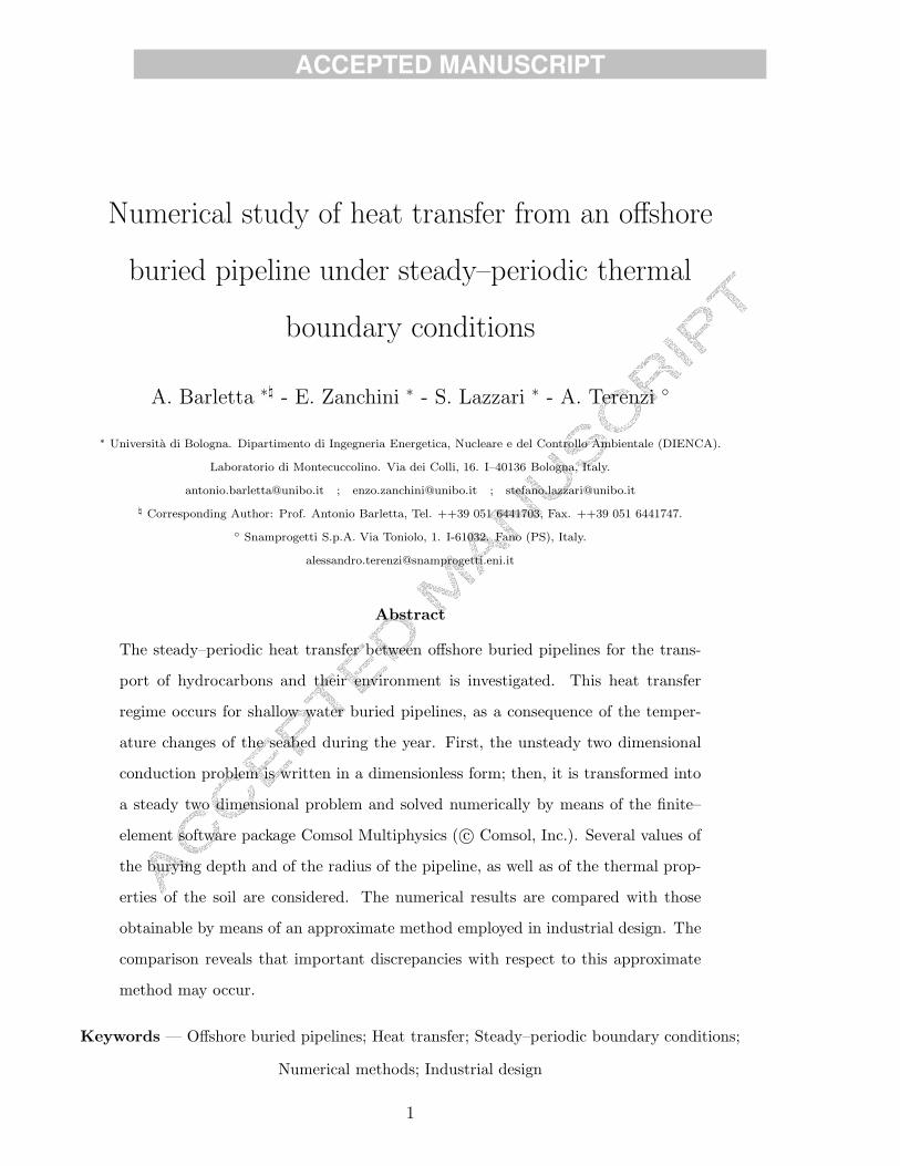
The steady–periodic heat transfer between offshore buried pipelines for the trans-
port of hydrocarbons and their environment is investigated. This heat transfer
regime occurs for shallow water buried pipelines, as a consequence of the temper-
ature changes of the seabed during the year. First, the unsteady two dimensional
conduction problem is written in a dimensionless form; then, it is transformed into
a steady two dimensional problem and solved numerically by means of the finite–
element software package Comsol Multiphysics ( c© Comsol, Inc.). Several values of
the burying depth and of the radius of the pipeline, as well as of the thermal prop-
erties of the soil are considered. The numerical results are compared with those
obtainable by means of an approximate method employed in industrial design. The
comparison reveals that important discrepancies with respect to this approximate
method may occur.
Keywords — Offshore buried pipelines; Heat transfer; Steady–periodic boundary conditions;
Numerical methods; Industrial design
1
ACCEPTED MANUSCRIPT
List of symbols
A, B dimensionless coefficients
a dimensionless length
C dimensionless constant defined in Eq.(A2)
cv soil specific heat at constant volume
H burying depth of the pipeline
k soil conductivity
~n normal unit vector
q thermal power per unit area
Q thermal power per unit length
Qconst thermal power per unit length, in the constant power limit
Qqs thermal power per unit length, in the quasi–stationary limit
R pipeline radius
Ta pipeline wall temperature
Te seabed temperature
Teff effective temperature
TH soil temperature at a depth H
Tm mean annual seabed temperature
T0, T1, T2 temperature fields
t time
X, Y coordinates
x, y dimensionless coordinates
Greek Symbols
α soil thermal diffusivity
β, γ dimensionless quantities defined in Eq.(A4)
∆T amplitude of temperature oscillations
θ0, θ1, θ2 dimensionless temperature fields
2
ACCEPTED MANUSCRIPT
Λ0 dimensionless heat transfer coefficient
Ξ dimensionless parameter
ρ soil density
σ dimensionless burying depth
Σ dimensionless parameter
φ phase angle defined in Eq.(A3)
ω angular frequency
Superscripts, subscripts
∗ dimensionless quantity
max maximum value
min minimum value
1 Introduction
As is well known, offshore buried pipelines are often used for the transport of hydrocar-
bons from extraction sites to refinement plants. The design of these pipelines requires
the knowledge of the overall heat transfer coefficient from the pipe wall to the environ-
ment. In fact, a significant decrease of the fluid temperature could cause the formation
of hydrates and waxes which might stop the fluid flow. Moreover, the knowledge of the
bulk temperature of the fluid in any cross section is necessary to determine the value of
the fluid viscosity in that section and, thus, to evaluate the viscous pressure drop along
the flow direction. As a consequence, the heat transfer from buried pipelines has been
widely studied in the literature [1]–[4]. An analytical expression of the steady–state heat
transfer coefficient from an offshore buried pipeline to its environment can be found in
[5]. It refers to the boundary condition of a uniform temperature of the seabed, i.e. of
the separation surface between soil and sea water. In these conditions, the thermal power
exchanged between the pipeline and its environment, per unit length of the duct, can be
3
ACCEPTED MANUSCRIPT
expressed as
Q = k (Ta − Te) Λ0 , (1)
where k is the thermal conductivity of the soil, Ta is the temperature of the external
surface of the duct, Te is the temperature of the seabed and Λ0 is a dimensionless heat
transfer coefficient, given by
Λ0 (σ) =2π
arccosh (σ). (2)
In Eq. (2), σ is the ratio between the burying depth of the pipe axis, H , and the external
radius of the pipe, R.
Equations (1) and (2) provide reliable results in many cases, but cannot be applied, for
instance, in the following circumstance. For shallow–water pipelines, the temperature of
the seabed is affected by the season changes and varies accordingly during the year. With
reference to the Mediterranean sea, the seabed statistically reaches a minimum value of
14C, in winter, and a maximum value of 25C, in summer. Clearly, this temperature
change of the seabed may have a strong influence on the thermal power exchanged be-
tween the pipeline and its environment.
At present, an approximate method is employed in industrial design to take into account
this effect. The soil is considered as a semi–infinite solid medium whose surface temper-
ature varies in time according to the law
T = Tm + ∆T sin (ω t) , (3)
where Tm is the mean annual temperature of the seabed, ∆T is the amplitude of the
temperature oscillation and ω is the angular frequency which corresponds to the period
of one year, namely
ω = 0.1991 · 10−6 s−1 . (4)
Thus, by assuming that the pipeline does not modify considerably the temperature dis-
tribution in the soil, at a depth H one has [6]
TH = Tm − ∆T exp
(
−
√
ω
2αH
)
sin
(√
ω
2αH − ω t
)
, (5)
4
ACCEPTED MANUSCRIPT
where α is the thermal diffusivity of the soil. In the approximate method, the thermal
power is evaluated as
Q = k (Ta − TH) Λ0 , (6)
i.e. by replacing Te with TH in Eq. (1).
The approximate method does not seem reliable because it is not based on a rigorous
mathematical model. To check the reliability of the method, one can apply it to eval-
uate the heat transfer between a plane isothermal surface buried at a depth H and the
surrounding soil, when the temperature of the ground surface varies in time according
to Eq.(3). In fact, for this case, an analytical expression of the soil temperature field is
available in the literature [7]. This analysis has been performed with reference to standard
properties of the soil and is reported in Appendix. The comparison between the analyti-
cal solution and the approximate method shows that the latter yields acceptable results
only when very small values of H are considered. Therefore, a more reliable method to
evaluate the steady–periodic heat transfer from buried pipelines to the environment is
needed.
The aim of this investigation is to find out an accurate method to determine the heat
transfer between an offshore buried pipeline and its environment in steady–periodic con-
ditions. First, by introducing suitable auxiliary variables, the unsteady two dimensional
conduction problem is transformed into a steady two dimensional problem in the new vari-
ables. Then, the steady problem is solved numerically by means of the software package
COMSOL Multiphysics ( c© Comsol, Inc.). The results show that the empirical method
given by Eqs. (6), (5) and (2) may yield a too rough approximation in some cases.
2 Mathematical model
Let us assume that the temperature of the seabed varies in time according to Eqs. (3) and
(4). The computational domain and the boundary conditions are sketched in Figure 1. As
is shown in the figure, the vertical and bottom boundaries of the computational domain
5
ACCEPTED MANUSCRIPT
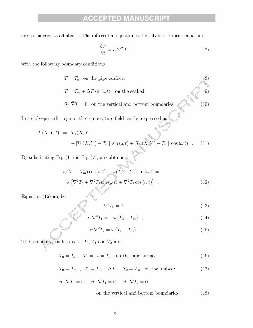
are considered as adiabatic. The differential equation to be solved is Fourier equation
∂T
∂t= α∇2 T , (7)
with the following boundary conditions:
T = Ta on the pipe surface; (8)
T = Tm + ∆T sin (ωt) on the seabed; (9)
~n · ~∇T = 0 on the vertical and bottom boundaries. (10)
In steady–periodic regime, the temperature field can be expressed as
T (X, Y, t) = T0 (X, Y )
+ [T1 (X, Y ) − Tm] sin (ω t) + [T2 (X, Y ) − Tm] cos (ω t) . (11)
By substituting Eq. (11) in Eq. (7), one obtains
ω (T1 − Tm) cos (ω t) − ω (T2 − Tm) sin (ω t) =
α[
∇2T0 + ∇2T1 sin (ω t) + ∇2T2 cos (ω t)]
. (12)
Equation (12) implies
∇2T0 = 0 , (13)
α∇2T1 = −ω (T2 − Tm) , (14)
α∇2T2 = ω (T1 − Tm) . (15)
The boundary conditions for T0, T1 and T2 are:
T0 = Ta , T1 = T2 = Tm on the pipe surface; (16)
T0 = Tm , T1 = Tm + ∆T , T2 = Tm on the seabed; (17)
~n · ~∇T0 = 0 , ~n · ~∇T1 = 0 , ~n · ~∇T2 = 0
on the vertical and bottom boundaries. (18)
6
ACCEPTED MANUSCRIPT
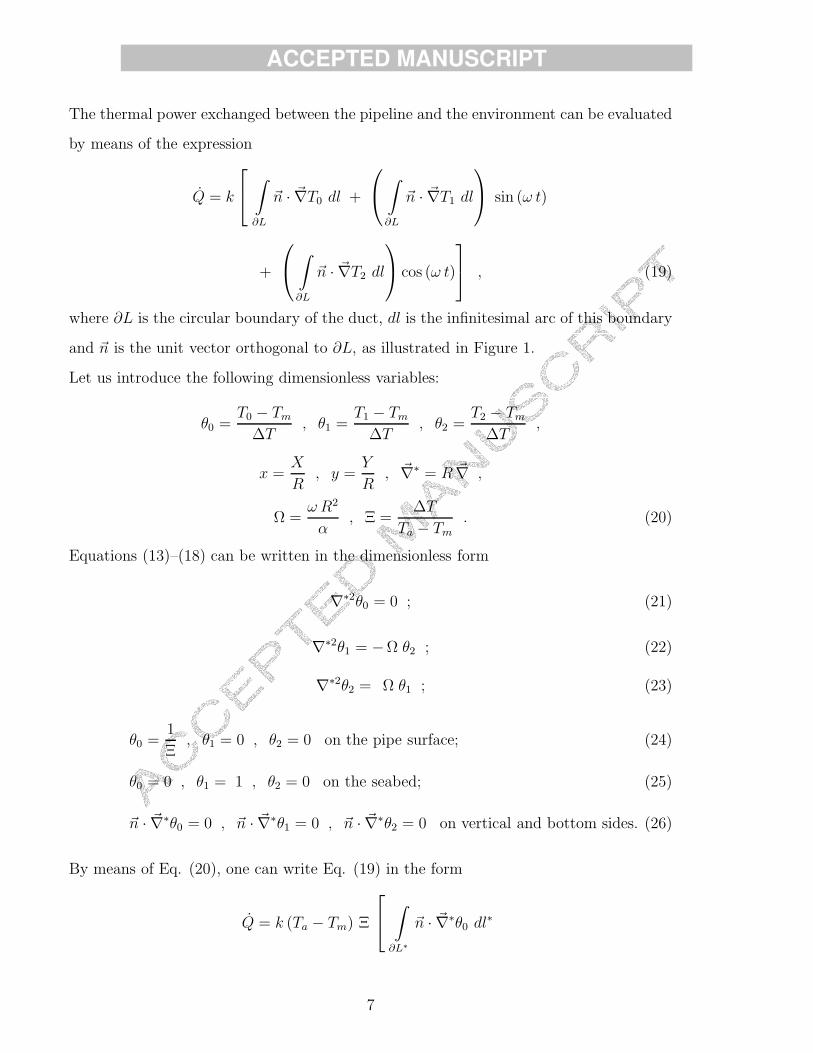
The thermal power exchanged between the pipeline and the environment can be evaluated
by means of the expression
Q = k
∫
∂L
~n · ~∇T0 dl +
∫
∂L
~n · ~∇T1 dl
sin (ω t)
+
∫
∂L
~n · ~∇T2 dl
cos (ω t)
, (19)
where ∂L is the circular boundary of the duct, dl is the infinitesimal arc of this boundary
and ~n is the unit vector orthogonal to ∂L, as illustrated in Figure 1.
Let us introduce the following dimensionless variables:
θ0 =T0 − Tm
∆T, θ1 =
T1 − Tm
∆T, θ2 =
T2 − Tm
∆T,
x =X
R, y =
Y
R, ~∇∗ = R ~∇ ,
Ω =ω R2
α, Ξ =
∆T
Ta − Tm
. (20)
Equations (13)–(18) can be written in the dimensionless form
∇∗2θ0 = 0 ; (21)
∇∗2θ1 = −Ω θ2 ; (22)
∇∗2θ2 = Ω θ1 ; (23)
θ0 =1
Ξ, θ1 = 0 , θ2 = 0 on the pipe surface; (24)
θ0 = 0 , θ1 = 1 , θ2 = 0 on the seabed; (25)
~n · ~∇∗θ0 = 0 , ~n · ~∇∗θ1 = 0 , ~n · ~∇∗θ2 = 0 on vertical and bottom sides. (26)
By means of Eq. (20), one can write Eq. (19) in the form
Q = k (Ta − Tm) Ξ
∫
∂L∗
~n · ~∇∗θ0 dl∗
7
ACCEPTED MANUSCRIPT
+
∫
∂L∗
~n · ~∇∗θ1 dl∗
sin (ω t) +
∫
∂L∗
~n · ~∇∗θ2 dl∗
cos (ω t)
. (27)
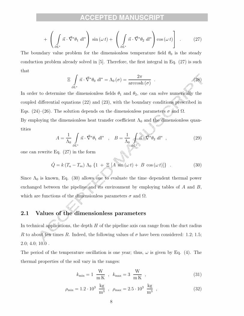
The boundary value problem for the dimensionless temperature field θ0 is the steady
conduction problem already solved in [5]. Therefore, the first integral in Eq. (27) is such
that
Ξ
∫
∂L∗
~n · ~∇∗θ0 dl∗ = Λ0 (σ) =2π
arccosh (σ). (28)
In order to determine the dimensionless fields θ1 and θ2, one can solve numerically the
coupled differential equations (22) and (23), with the boundary conditions prescribed in
Eqs. (24)–(26). The solution depends on the dimensionless parameters σ and Ω.
By employing the dimensionless heat transfer coefficient Λ0 and the dimensionless quan-
tities
A =1
Λ0
∫
∂L∗
~n · ~∇∗θ1 dl∗ , B =1
Λ0
∫
∂L∗
~n · ~∇∗θ2 dl∗ , (29)
one can rewrite Eq. (27) in the form
Q = k (Ta − Tm) Λ0 1 + Ξ [A sin (ω t) + B cos (ω t)] . (30)
Since Λ0 is known, Eq. (30) allows one to evaluate the time–dependent thermal power
exchanged between the pipeline and its environment by employing tables of A and B,
which are functions of the dimensionless parameters σ and Ω.
2.1 Values of the dimensionless parameters
In technical applications, the depth H of the pipeline axis can range from the duct radius
R to about ten times R. Indeed, the following values of σ have been considered: 1.2; 1.5;
2.0; 4.0; 10.0 .
The period of the temperature oscillation is one year; thus, ω is given by Eq. (4). The
thermal properties of the soil vary in the ranges:
kmin = 1W
m K, kmax = 3
W
m K, (31)
ρmin = 1.2 · 103 kg
m3, ρmax = 2.5 · 103 kg
m3, (32)
8
ACCEPTED MANUSCRIPT
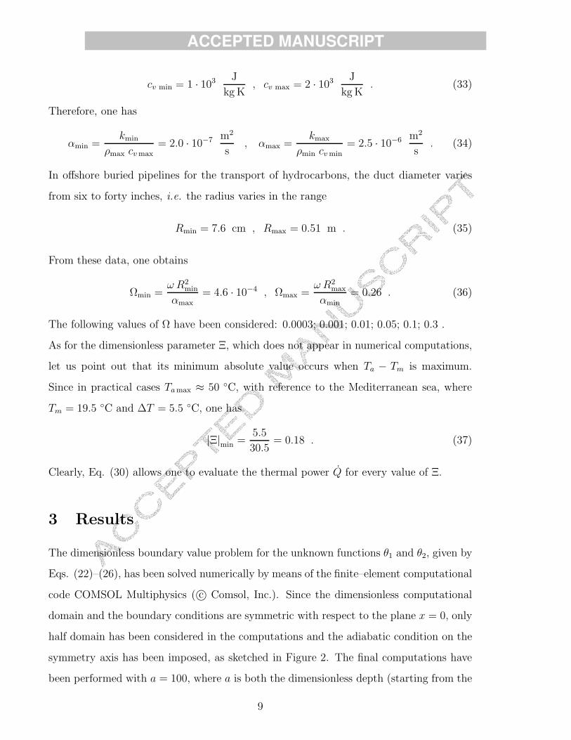
cv min = 1 · 103 J
kg K, cv max = 2 · 103 J
kg K. (33)
Therefore, one has
αmin =kmin
ρmax cv max= 2.0 · 10−7 m2
s, αmax =
kmax
ρmin cv min= 2.5 · 10−6 m2
s. (34)
In offshore buried pipelines for the transport of hydrocarbons, the duct diameter varies
from six to forty inches, i.e. the radius varies in the range
Rmin = 7.6 cm , Rmax = 0.51 m . (35)
From these data, one obtains
Ωmin =ω R2
min
αmax
= 4.6 · 10−4 , Ωmax =ω R2
max
αmin
= 0.26 . (36)
The following values of Ω have been considered: 0.0003; 0.001; 0.01; 0.05; 0.1; 0.3 .
As for the dimensionless parameter Ξ, which does not appear in numerical computations,
let us point out that its minimum absolute value occurs when Ta − Tm is maximum.
Since in practical cases Ta max ≈ 50 C, with reference to the Mediterranean sea, where
Tm = 19.5 C and ∆T = 5.5 C, one has
|Ξ|min =5.5
30.5= 0.18 . (37)
Clearly, Eq. (30) allows one to evaluate the thermal power Q for every value of Ξ.
3 Results
The dimensionless boundary value problem for the unknown functions θ1 and θ2, given by
Eqs. (22)–(26), has been solved numerically by means of the finite–element computational
code COMSOL Multiphysics ( c© Comsol, Inc.). Since the dimensionless computational
domain and the boundary conditions are symmetric with respect to the plane x = 0, only
half domain has been considered in the computations and the adiabatic condition on the
symmetry axis has been imposed, as sketched in Figure 2. The final computations have
been performed with a = 100, where a is both the dimensionless depth (starting from the
9
ACCEPTED MANUSCRIPT
pipeline axis) and the dimensionless width of the actual computational domain, as shown
in Figure 2. Indeed, preliminary calculations revealed that this value of a is sufficiently
high to ensure accurate results.
Unstructured grids with triangular elements have been used. The grids have been refined
close to the boundaries 1, 6 and 5, and in a square region around the duct (see Figure
3). After some checks to ensure the grid–independence, the final computations have been
performed with about 5 · 104 grid elements.
The values of the coefficients A and B given by Eq. (29) are determined by COMSOL
Multiphysics as follows. The x–component and the y–component of the gradient of θ1 and
θ2 are multiplied by the x–component and y–component of the unit vector normal to the
boundary surface 5 (see Figure 2). The latter components are built–in variables denoted
as nx and ny. Then, A and B are evaluated in postprocessing through the Boundary
Integration option.
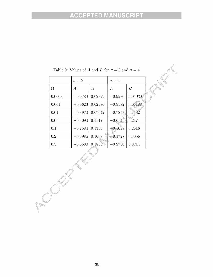
The results obtained for the coefficients A and B are reported in Table 1 for σ = 1.2 and
σ = 1.5, in Table 2 for σ = 2 and σ = 4, in Table 3 for σ = 6 and σ = 10.
In order to illustrate the effects of the temperature oscillations at the seabed on the heat
transfer rate between the pipe and its environment, let us compare the thermal power
exchanged in steady–periodic regime, given by Eq. (30), with two limiting cases. In the
limit of very high values of H and very low values of α, i.e. for very high values of both
σ and Ω, the effect of the temperature oscillations at the seabed on the heat transfer
rate becomes negligible. In this limit, which will be called constant power limit, the sea
temperature oscillations affect only a thin soil layer close to the seabed, far from the pipe,
so that the thermal power exchanged between the pipeline and its environment is constant
and is given by
Qconst = k (Ta − Tm) Λ0 . (38)
On the other hand, in the limit of σ very close to 1 and of very low values of Ω, one
can assume that the temperature oscillations have a uniform phase. In this limit, which
will be called quasi–stationary limit, the thermal power exchanged between pipeline and
environment can be evaluated, at any time instant, by considering steady–state conditions
10
ACCEPTED MANUSCRIPT
with a temperature at the seabed given by the temperature at that instant. Thus, in the
quasi–stationary limit, one has
Qqs = k (Ta − Tm) Λ0 [1 − Ξ sin (ω t)] . (39)
A comparison between Eqs. (30) and (38) reveals that the general expression for the
steady–periodic thermal power coincides with Qconst (constant power limit) when A =
B = 0. A comparison between Eqs. (30) and (39) reveals that the general expression
for the steady–periodic thermal power coincides with Qqs (quasi-stationary limit) when
A = −1 and B = 0. Indeed, the results reported in Table 3 point out that, for σ = 10
and Ω = 0.3, the values of A and B are very close to zero, i.e. the constant power limit
is approached. On the other hand, the results reported in Table 1 point out that, for
σ = 1.2 and Ω = 0.0003, A ≈ −1 and B ≈ 0, so that the quasi–stationary limit is nearly
reached.
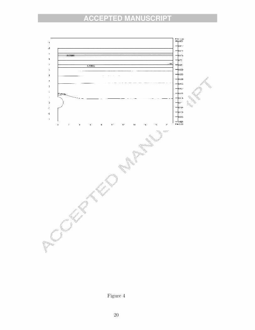
The amplitude of the dimensionless temperature oscillations√
θ21 + θ2
2 is illustrated in
Figure 4 for σ = 10 and Ω = 0.3. The figure shows that the temperature oscillations are
negligible at the depth of the pipe, so that a nearly constant heat flux from the duct wall
occurs (constant power limit).
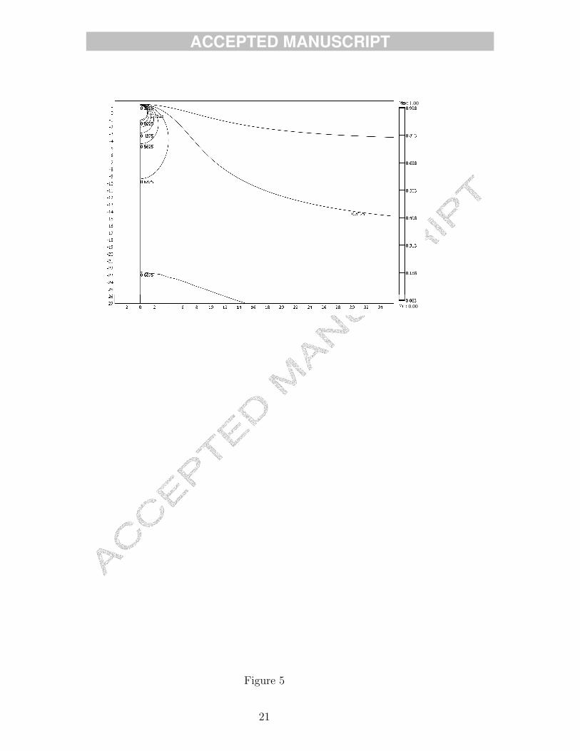
The amplitude√
θ21 + θ2
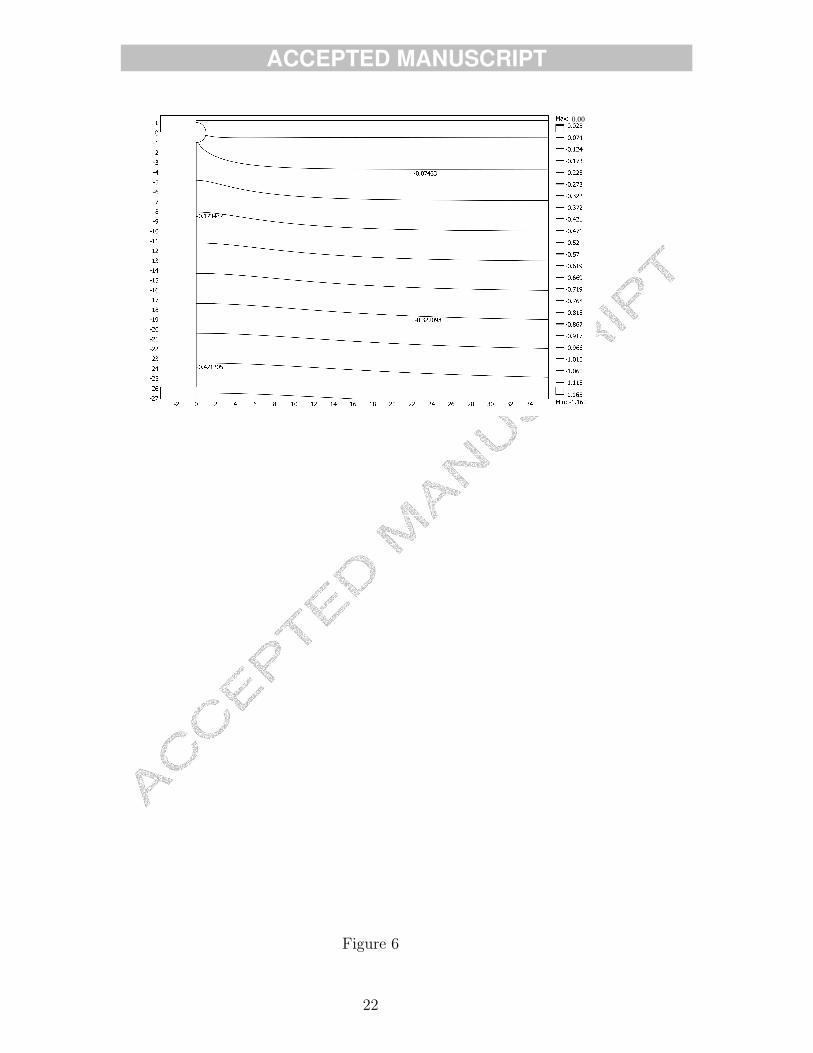
2 and the phase arctan (θ2 /θ1) of the dimensionless temperature
oscillations, for σ = 1.2 and Ω = 0.0003, are illustrated in Figures 5 and 6 respectively.
Figure 5 shows that important temperature oscillations take place in the soil even at
depths greater than that of the pipe, except very close to the pipe boundary, where a
constant temperature boundary condition has been imposed.
Figure 6 shows that the phase is nearly uniform and next to zero even at depths higher
than that of the pipe. Thus, the quasi–stationary limit can be applied with an excellent
approximation in this case. In most cases, neither the constant power limit not the
quasi–stationary limit can be applied, and the power exchanged between the pipe and its
environment must be calculated by means of Eq. (30) and of Tables 1, 2 and 3.
In order to compare the results presented in this paper with the approximate results
11
ACCEPTED MANUSCRIPT
obtainable by means of Eq. (6), let us rewrite Eq. (30) in the form
Q = k (Ta − Teff ) Λ0 , (40)
where the effective temperature Teff is given by
Teff = Tm − ∆T [A sin (ω t) + B cos (ω t)] . (41)
Clearly, Eq. (6) agrees with Eq. (40) if TH coincides with Teff . From Eqs. (5) and (20),
one obtains
TH = Tm − ∆T exp
(
−σ
√
Ω
2
) [
− cos
(
σ
√
Ω
2
)
sin (ω t)
+ sin
(
σ
√
Ω
2
)
cos (ω t)
]
. (42)
Equations (41) and (42) show that TH coincides with Teff if
A = − cos
(
σ
√
Ω
2
)
exp
(
−σ
√
Ω
2
)
, (43)
B = sin
(
σ
√
Ω
2
)
exp
(
−σ
√
Ω
2
)
. (44)
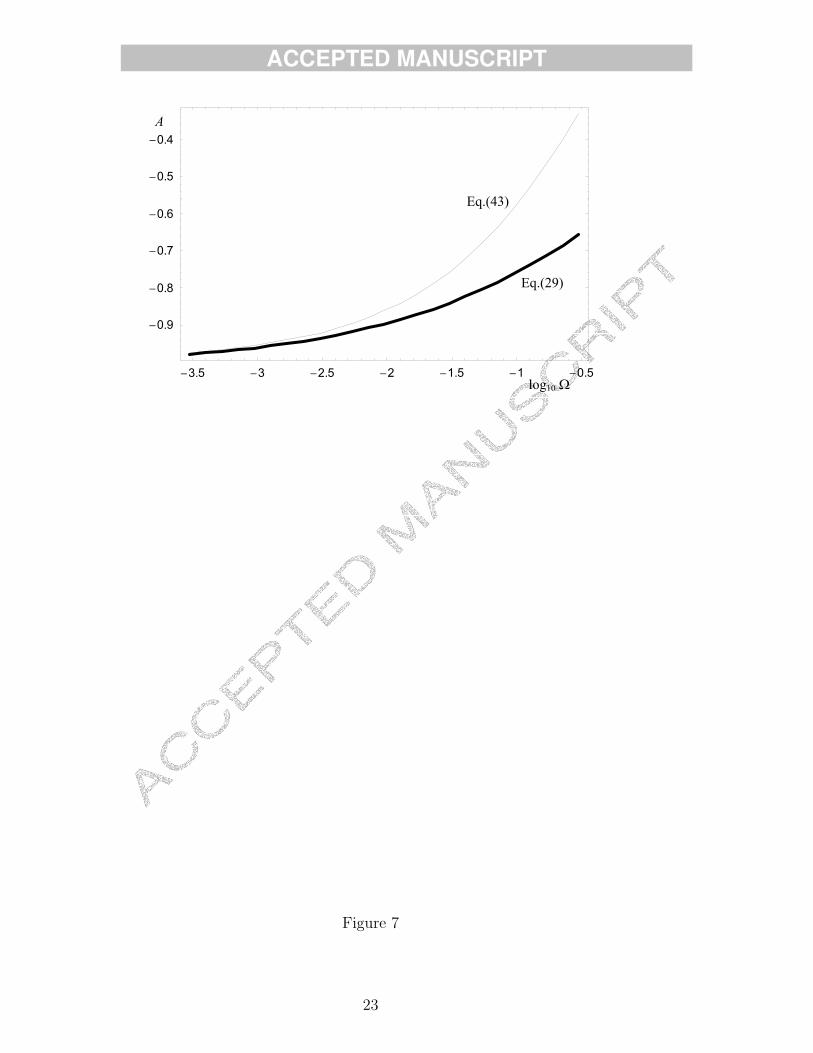
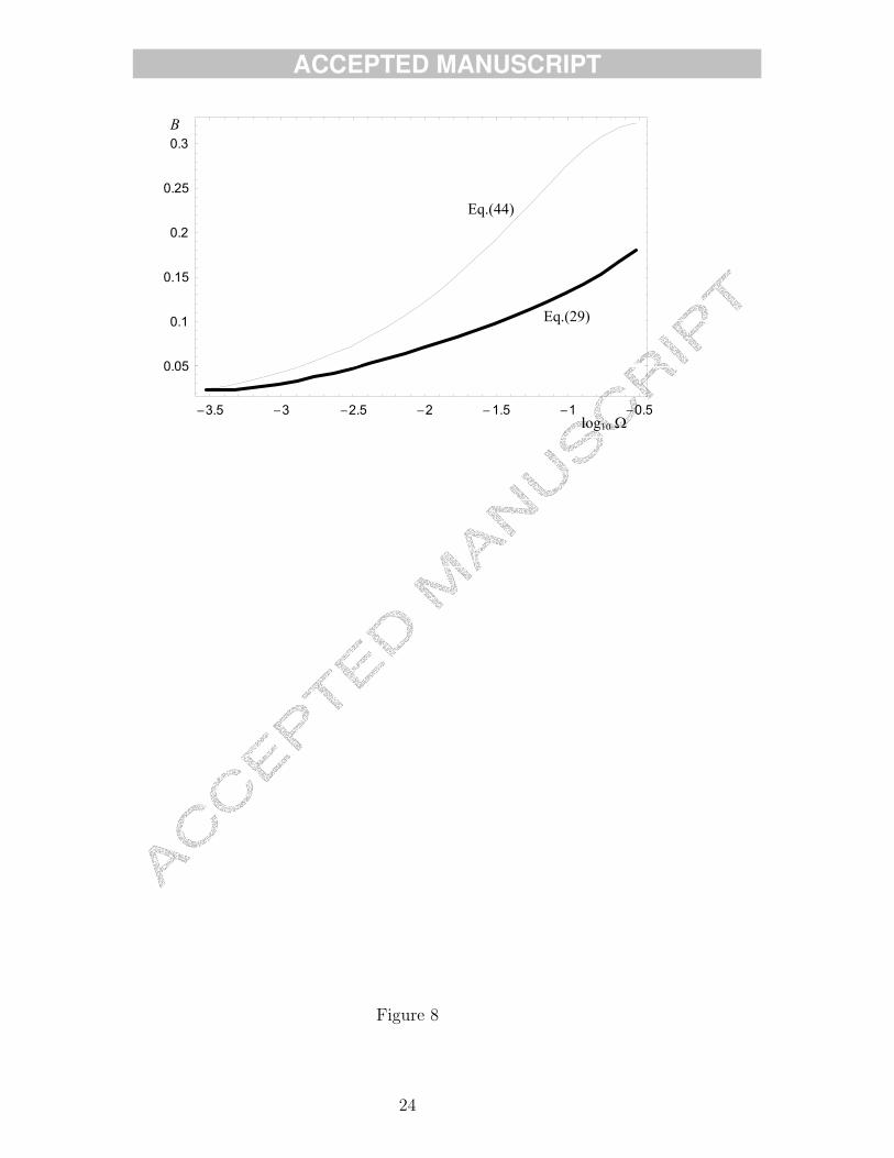
A comparison between the values of A and B obtained numerically in this paper and
the approximate values given by Eqs. (43) and (44) is illustrated in Figures 7 and 8,
where A and B are plotted versus the logarithm base 10 of Ω, for σ = 2, in the range
0.0003 ≤ Ω ≤ 0.3. The figures show that a strong disagreement between the correct and
the approximate values of A and B occurs, for high values of Ω. Therefore, the naive
method employed in industrial design may yield a too rough approximation, except for
very low values of Ω.
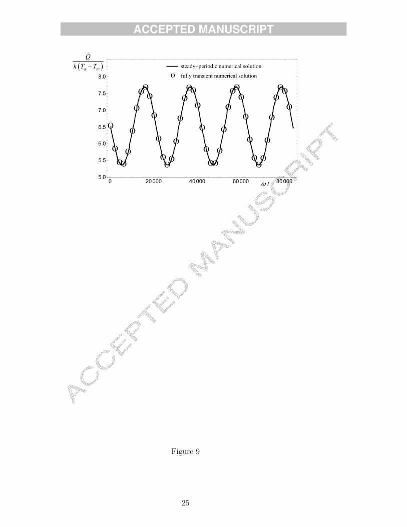
A check has been made on the steady–periodic numerical solution, namely a comparison
with the fully transient numerical solution of Eqs.(7)–(10). The latter numerical solution
has been also performed by Comsol Multiphysics by means of the Time Dependent solver.
The initial condition considered is a uniform temperature distribution in the soil with
value Tm. The solution has been obtained in the dimensionless domain by using the
12
ACCEPTED MANUSCRIPT
values Ω = 3× 10⁻⁴, Ξ = 0.18, σ = 1.5. In Figure 9, Q/[k (Ta − Tm)] versus ωt is plotted
in this case either using Eqs. (29) and (30) (solid line) or using the fully transient solution
(dots). Figure 9 shows that the numerical solutions are in perfect agreement. In fact, the
effect of the initial condition decays very rapidly and becomes negligible when ωt > 100.
4 Conclusions
The steady–periodic heat transfer between buried offshore pipelines and their environ-
ment has been studied. The unsteady two dimensional conduction problem has been
transformed into a steady two dimensional problem and solved numerically by means
of the finite–element software package COMSOL Multiphysics ( c© Comsol Inc.). The
results, reported through tables containing the values of two dimensionless parameters,
can be employed for a wide range of values of the burying depth and of the radius of
the pipeline, as well as of the thermal properties of the soil. The results obtained have
been compared with those predicted by an approximate method employed in industrial
design. The comparison revealed that the approximate method may be unreliable in some
design conditions corresponding to a large diameter of the pipeline and to a low thermal
diffusivity of the soil.
References
[1] A. Terenzi, F. Terra, External heat transfer coefficient of a partially sunken sealine,
International Communications in Heat and Mass Transfer 28 (2001) 171–179.
[2] D. Hatziavramidis, H.-C. Ku, Pseudospectral solutions of laminar heat transfer
problems in pipelines, Journal of Computational Physics 52 (1983) 414–424.
[3] A. Chervinsky, Y. Manheimer-Timnata, Transfer of liquefied natural gas in long
insulated pipelines, Criogenics 9 (1969) 180–185.
13
ACCEPTED MANUSCRIPT
[4] S. D. Probert, C. Y. Chu, Laminar flows of heavy-fuel oils through internally insu-
lated pipelines, Applied Energy 15 (1983) 81–98.
[5] V. J. Lunardini, Heat Transfer in Cold Climates, Van Nostrand Reinhold Co, New
York, 1981.
[6] A. N. Tichonov, A. A. Samarskij, Equazioni della Fisica Matematica, Mir, Mosca,
1981.
[7] H. S. Carslaw, J. C. Jaeger, Conduction of heat in solids, Oxford University Press,
Glasgow, 1947, Chapter III.
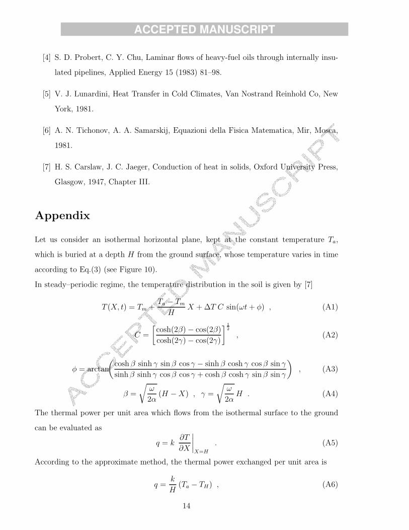
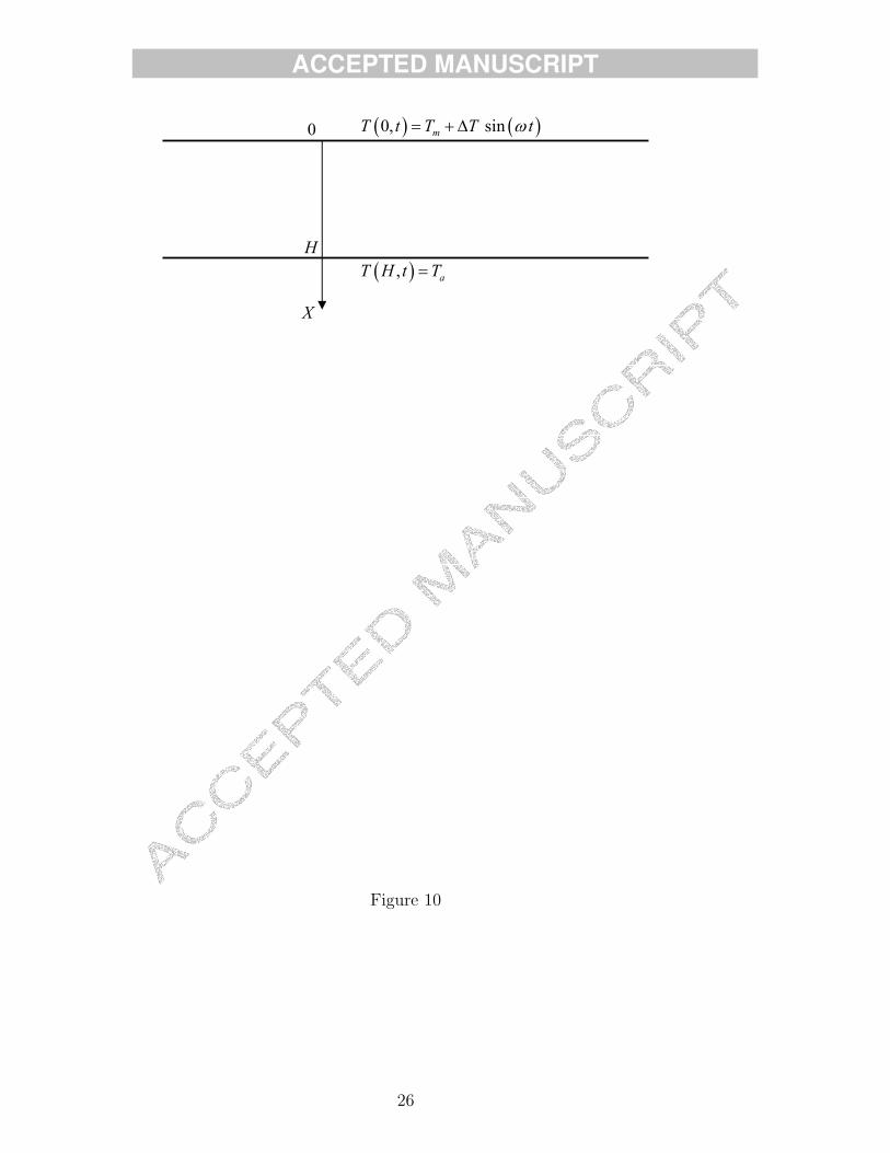
Appendix
Let us consider an isothermal horizontal plane, kept at the constant temperature Ta,
which is buried at a depth H from the ground surface, whose temperature varies in time
according to Eq.(3) (see Figure 10).
In steady–periodic regime, the temperature distribution in the soil is given by [7]
T (X, t) = Tm +Ta − Tm
HX + ∆T C sin(ωt + φ) , (A1)
C =
[
cosh(2β) − cos(2β)
cosh(2γ) − cos(2γ)
]1
2
, (A2)
φ = arctan
(
cosh β sinh γ sin β cos γ − sinh β cosh γ cos β sin γ
sinh β sinh γ cos β cos γ + cosh β cosh γ sin β sin γ
)
, (A3)
β =
√
ω
2α(H − X) , γ =
√
ω
2αH . (A4)
The thermal power per unit area which flows from the isothermal surface to the ground
can be evaluated as
q = k∂T
∂X
∣
∣
∣
∣
X=H
. (A5)
According to the approximate method, the thermal power exchanged per unit area is
q =k
H(Ta − TH) , (A6)
14
ACCEPTED MANUSCRIPT
where TH is given by Eq.(5).
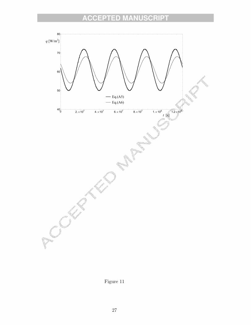
Let us assume Ta = 50 C , Tm = 19.5 C , ∆T = 5.5 C and consider a soil with the
following thermal properties: k = 2 W/(m K) , α = 5 · 10−7 m2/s. A comparison of the
thermal power per unit area given by Eq.(A5) and that given by Eq.(A6) is illustrated in
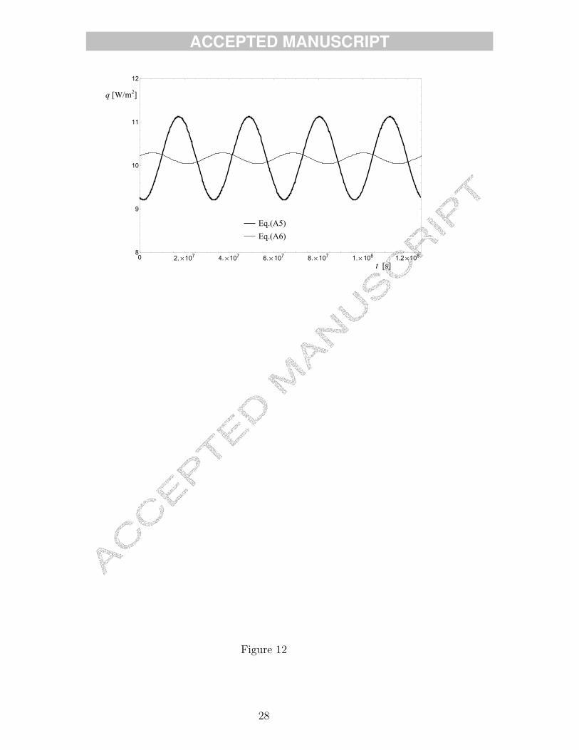
Figure 11 for H = 1 m and in Figure 12 for H = 6 m. In both Figures, the thin line refers
to Eq.(A6) (approximate method), while the thick line refers to the analytical solution,
given by Eq.(A5). The Figures show that while for H = 1 m the results of the approx-
imate method can be considered as acceptable, for H = 6 m the approximate method
underestimates the amplitude of the fluctuations of the thermal power and predicts a
wrong phase of these oscillations.
15
ACCEPTED MANUSCRIPT
Figure captions
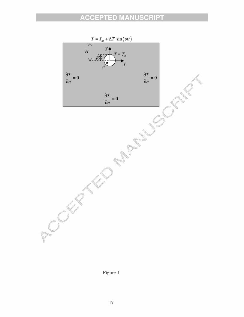
Figure 1 – Computational domain and boundary conditions.
Figure 2 – Dimensionless computational domain and boundary conditions.
Figure 3 – The unstructured grid adopted together with a magnification of the refinement
made near the pipeline
Figure 4 – Amplitude of the dimensionless temperature oscillations for σ = 10 and
Ω = 0.3.
Figure 5 – Amplitude of the dimensionless temperature oscillations for σ = 1.2 and
Ω = 0.0003.
Figure 6 – Phase of the dimensionless temperature oscillations for σ = 1.2 and Ω =
0.0003.
Figure 7 – Plots of A versus log10 Ω for σ = 2, according to Eq.(29) (thick line) and to
Eq. (44) (thin line).
Figure 8 – Plots of B versus log10 Ω for σ = 2, according to Eq.(29) (thick line) and to
Eq. (44) (thin line).
Figure 9 – Values of Q/[k (Ta −Tm)] versus ωt. Comparison between the steady–periodic
numerical solution and the fully transient numerical solution.
Figure 10 – Isothermal horizontal plane buried at a depth H. The temperature of the
ground surface in X = 0 varies according to Eq.(3).
Figure 11 – Plots of the thermal power q exchanged per unit area versus time t, for
H = 1m, according to the analytical solution given by Eq.(A5) (thick line) and to the
approximate method given by Eq.(A6) (thin line).
Figure 12 – Plots of the thermal power q exchanged per unit area versus time t, for
H = 6m, according to the analytical solution given by Eq.(A5) (thick line) and to the
approximate method given by Eq.(A6) (thin line).
16
ACCEPTED MANUSCRIPT
T = Ta
0T
n
∂=
∂
n
Y
0T
n
∂=
∂
0T
n
∂=
∂
X
( )sinm
T T T t= + ∆ ω
R
H
Figure 1
17

ACCEPTED MANUSCRIPT
σ
24
5
6
11θ = 2
0θ =
10
n*
∂θ=
∂
20
n*
∂θ=
∂
10
n*
∂θ=
∂
20
n*
∂θ=
∂a
a
x
y
1
1
3
10θ =
20θ =
10
n*
∂θ=
∂
20
n*
∂θ=
∂
Figure 2
18

ACCEPTED MANUSCRIPT
Figure 3
19
ACCEPTED MANUSCRIPT
1.00
0.00
Figure 4
20
ACCEPTED MANUSCRIPT
1.00
0.00
Figure 5
21
ACCEPTED MANUSCRIPT
0.00
Figure 6
22
ACCEPTED MANUSCRIPT
3.5 3 2.5 2 1.5 1 0.5
0.9
0.8
0.7
0.6
0.5
0.4
A
log10
Eq.(43)
Eq.(29)
Figure 7
23
ACCEPTED MANUSCRIPT
3.5 3 2.5 2 1.5 1 0.5
0.05
0.1
0.15
0.2
0.25
0.3
B
log10
Eq.(44)
Eq.(29)
Figure 8
24
ACCEPTED MANUSCRIPT
O
O
OO
O
O
O
OOO
O
O
OO
O
O
O
O
OO
O
O
O
OO
O
O
O
OO
O
O
O
OO
O
O
O
O
OO
O
0 20000 40000 60000 800005.0
5.5
6.0
6.5
7.0
7.5
8.0
8.5
t
a m
Q
k T T steady periodic numerical solution
fully transient numerical solution O
Figure 9
25
ACCEPTED MANUSCRIPT
0, sin
mT t T T t
,a
T H t T
X
H
0
Figure 10
26
ACCEPTED MANUSCRIPT
0 2. 107
4. 107
6. 107
8. 107
1. 108
1.2 108
40
50
60
70
80
q [W/m2]
t [s]
Eq.(A5)
Eq.(A6)
Figure 11
27
ACCEPTED MANUSCRIPT
0 2. 107
4. 107
6. 107
8. 107
1. 108
1.2 108
8
9
10
11
12
q [W/m2]
t [s]
Eq.(A5)
Eq.(A6)
Figure 12
28

ACCEPTED MANUSCRIPT
Table 1: Values of A and B for σ = 1.2 and σ = 1.5.
σ = 1.2 σ = 1.5
Ω A B A B
0.0003 −0.9920 0.009141 −0.9863 0.01526
0.001 −0.9855 0.01186 −0.9754 0.01971
0.01 −0.9592 0.02889 −0.9321 0.04738
0.05 −0.9224 0.04590 −0.8722 0.07501
0.1 −0.9010 0.05424 −0.8376 0.08915
0.2 −0.8762 0.06358 −0.7973 0.1058
0.3 −0.8599 0.06984 −0.7707 0.1175
29
ACCEPTED MANUSCRIPT
Table 2: Values of A and B for σ = 2 and σ = 4.
σ = 2 σ = 4
Ω A B A B
0.0003 −0.9789 0.02329 −0.9530 0.04930
0.001 −0.9623 0.02986 −0.9182 0.06188
0.01 −0.8970 0.07042 −0.7857 0.1382
0.05 −0.8090 0.1112 −0.6145 0.2174
0.1 −0.7584 0.1333 −0.5098 0.2616
0.2 −0.6986 0.1607 −0.3728 0.3056
0.3 −0.6580 0.1803 −0.2730 0.3214
30

ACCEPTED MANUSCRIPT
Table 3: Values of A and B for σ = 6 and σ = 10.
σ = 6 σ = 10
Ω A B A B
0.0003 −0.9287 0.07171 −0.8816 0.1105
0.001 −0.8784 0.08875 −0.8050 0.1345
0.01 −0.6906 0.1908 −0.5193 0.2696
0.05 −0.4435 0.2895 −0.1389 0.3095
0.1 −0.2833 0.3210 0.03150 0.2136
0.2 −0.09150 0.2974 0.08847 0.06089
0.3 0.01094 0.2381 0.06136 −0.001761
31