1275

NUMERICAL STUDY OF DISPERSION AND NONLINEARITY EFFECTS ON TSUNAMI PROPAGATION

Alwafi Pujiraharjo1 and Tokuzo Hosoyamada2

Numerical study of dispersion effect for tsunami propagation for the case of Indian

Ocean Tsunami has been carried out using three model equations: Linear shallow water

(LSW) equations, Nonlinear shallow water (NLSW) equations, and Weakly-Nonlinear

Bossuineq-type (WNB) equations. Model simulation results are compared each other and

against observations data. General features of tsunami wave patterns are agree very well

using the three models but the WNB model produced development in time of tsunami

front face which caused by the dispersion effect. Two dimensional wave pattern and

spatial profile of sea surface are discussed to study the dispersion effect.

INTRODUCTION

Indian Ocean Tsunami (IOT) of 26 December 2004 is recorded as highest

tsunami. Triggered by tectonic earthquake, the tsunami waves are generated by a

complicated bottom uplift/downlift with multiple components of amplitude and

frequency. The tsunami was globally propagated over the world ocean as trans-

oceanic tsunami propagation. Very complicated structures of spatial and

temporal waves are observed by many researchers. For trans-oceanic tsunami

propagation, dispersion effect could be significant factor for prediction of

maximum amplitude. Kulikov (2005) reported the dispersion effect tsunami

waves in the Indian Ocean from wavelet analysis using satellite data record. In

the coastal area tsunami waves interact with very complicated bathymetry. Hence,

model equations which include both dispersive and nonlinear terms are needed

for better estimation.

Preliminary results of dispersive numerical model of IOT has been done by

Watts et al. (2005) using Boussinesq-type model. More detail study of dispersion

effect for IOT has been conducted using nonlinear shallow water, nonlinear

Boussinesq and the full nonlinear Navier-Stokes models by Horillo et al. (2006).

Grilli et al. (2007) also discussed the dispersion effect for IOT event. From the

discussions, the dispersion effect is noticed at the south-west direction, while at

the east part tsunami is essentially nondispersive.

The aims of this study is to reproduce simulation of IOT using three

different model equations as tools to study the dispersion effect of IOT at the

initial stage (up to 3 hours tsunami propagation). The models results are compare

each other and against observed data.

1 Department of Civil Engineering, Brawijaya University, Jln. MT Haryono 167, Malang, 65145, INDONESIA

2 Department of Civil and Environment Engineering, Nagaoka University of Technology, 1603 -1 Kamitomioka-machi, Nagaoka, Niigata, 940-2188, JAPAN

1276 COASTAL ENGIEERING 2008

MODEL EQUATIONS AND NUMERICAL SOLUTION

Description of model equations

Three sets of model equations are used here i.e.: a simple linear shallow

water (LSW) equations, nonlinear shallow water (NLSW) equations, and

extended weakly nonlinear Boussinesq-type (WNB) equations of Nwogu (1993).

Time-dependent of water depth (bottom) term is included to the models based on

derivation of Lynett and Liu (2002). By including the time-dependent water

depth, the models could be implemented to simulate tsunami generation by

tectonic plate motions, earthquakes and underwater landslides. The sets of model

equations contain equation for conservation of mass and momentum

conservation are taken in the following form

( ) ( ) ( )

( ) ( )

2 21 10 1 2 6

1

2( ) 0

t t

t

h h z h h

z h h h h

η + + ∇ ⋅ + γ η + γ ∇ ⋅ − ∇ ∇ ⋅

+ + ∇ ∇ ⋅ + =

u u

u

ɶ ɶɶ

ɶɶ

(1)

( ) ( )210 2( ) ( ) 0

t t b brt

g z z h h + ∇η + γ ⋅∇ + ∇ ∇ ⋅ + ∇ ∇ ⋅ + + − =

u u u u u F Fɶ ɶ ɶ ɶ ɶɶ ɶ (2)

where h is the still water depth, η is free surface elevation, g is the gravitational

acceleration, while h is time dependent water depth. Subscript t denotes partial

derivative with respect to time. Two-dimensional vector differential operator ∇

is defined by ( ),x y

∂ ∂∂ ∂

∇ = .

Equations (1) and (2) are full form of model equations used here. Setting

variables γ0 = γ1 = 1 and horizontal velocity vector ( , )u v=uɶ ɶ ɶ as velocity at an

arbitrary level, zɶ , reduces the model equations to WNB model equations in

which zɶ is recommended to be 0.531z h= −ɶ (Nwogu, 1993). Then setting γ0 = 1

and γ1 = 0 and using depth averaged horizontal velocity vector ( , )u v=uɶ i.e. by

taking 0z =ɶ yields the NLSW model equations. The LSW model equations

could be obtained by using depth averaged horizontal velocity vectors and

neglecting the nonlinear terms (γ0 = γ1 = 0).

The Fb and Fbr terms in (2) are the additional terms to accommodate bottom

friction and energy dissipation caused by breaking waves, respectively. The

bottom friction terms are given in quadratic formula. Although the friction

coefficient should be a function of bottom roughness and velocity profile but a

simple constant friction coefficient is used in this study. Eddy viscosity formula

is used to model the turbulent mixing and energy dissipation caused by breaking

waves. Treatment of wave breaking is similar to the eddy viscosity-type formula

proposed by Kennedy et al. (2000) and Chen et al. (2000).

COASTAL ENGINEERING 2008 1277

Numerical solution

In order to eliminate the error terms to the same form of dispersive terms in

the WNB model equations, fourth-order accuracy of numerical scheme for time

stepping and first-order spatial derivatives are used (Wei and Kirby, 1995). High

order predictor-corrector scheme is used for time stepping, employing third

order time explicit Adam-Bashforth scheme as predictor and fourth order Adam-

Moulton implicit scheme as corrector step. The corrector step must be iterated

until a convergence criterion is satisfied. The system equations are written in a

form that makes convenient for application high-order time stepping procedure

(see Appendix or Wei and Kirby, 1995).

A staggered grid system (C grid) in space is used to discretize spatial

derivatives as shown in Fig. 1. The horizontal velocity vectors (u, v) and sea

level (η) are organized into triplets as visualized by triangle in Fig. 1. The water

depth is defined at the same point of sea level at the cell center, while vectors

such as velocity components u and v are defined at the interfaces of the cell. At

the cell interface, scalars are obtained by linear interpolation. For example, the

total water depth at u point can be obtained by

( ) ( ) ( )1 1, , 1, 1,2 2

,i j i j i j i j

i jh h h + ++ η = + η + + η (3)

Spatial discretizations are required for various orders of spatial derivatives on

the right-hand side of (A-1) which include first-order, second-order and second-

i

i+1

i-1

j

j-1

j+1

∆x

∆y

(η, h)i,j

ui,j

vi,j

Fig. 1 Staggered grid system for spatial discretization

1278 COASTAL ENGIEERING 2008

order cross derivatives. The first-order derivative of ( )f h u= + η in the x

direction is discretized by four-point finite difference method to eliminates fifth-

order physical dispersion in the governing equations as follows

( )2, 1, , 1,

,

127 27

24i j i j i j i j

i j

ff f f f

x x− − +

∂ = − + −

∂ ∆ (4)

The fourth-order accurate for first-order space derivative of η at u-point is

( )1, , 1, 2,

,

127 27

24i j i j i j i j

i jx x

− + +

∂η = η − η + η − η

∂ ∆ (5)

And the first-order derivative of u2 in the x direction is discretized by the

following scheme

2

2 2 2 2

2, 1, 1, 2,

,

1( ) 8( ) 8( ) ( )

12i j i j i j i j

i j

uu u u u

x x− − + +

∂ = − + − ∂ ∆

(6)

Three-point central scheme is used for second order derivatives in the x direction

as

2

1, , 1,2 2

,

12

i j i j i j

i j

ww w w

x x− +

∂ = − + ∂ ∆

(7)

where w = u or (hu). Similar expressions can be obtained in the y direction for

both first-order and second-order derivatives. The cross-derivative terms in the x

direction of uxy and (hu)xy are approximated by the following finite difference

scheme

2

1, , 1 1, 1 ,

,

1i j i j i j i j

i j

ww w w w

x y x y− + − +

∂ = + − − ∂ ∂ ∆ ∆

(8)

Again, w = u or (hu) and similar expressions can be obtained in the y direction

for vxy and (hv)xy.

NUMERICAL SIMULATION AND DISCUSSIONS

Simulation domain

The numerical models are then applied to make simulation of Indian Ocean

Tsunami event. In order to minimize the grid size and achieves resolution but

accommodate gauges and satellite data, numerical domain is selected around

Bay of Bengal from longitude 700E – 100

0E and latitude 7

0S – 23

0N. Bathymetry

data is taken from ETOPO2 databank and refined into one minute resolution by

linear interpolation resulting 1800 by 1800 of grid points. The mean water level

specified in the model simulation did not include the effects of tides. Spherical

and Coriolis effects also did not include in the models computation.

Radiation boundaries are applied at the south, west and east part of

numerical domain by adding sponge layers at the corresponding boundaries.

COASTAL ENGINEERING 2008 1279

Artificial slot technique for treatment ‘wet-dry’ condition for runup of Chen et al.

(2000) and Kennedy et al. (2000) is used here. The continuity equation (1) must

be modified to implement the artificial slot. Detail of implementation of artificial

slot technique for runup treatment is referred to Kennedy et al. (2000) and Chen

et al. (2000). Constant bottom friction coefficients of 0.001 and 0.0 are applied

when the water depth less and greater than 1 km, respectively.

Tsunami generation

Grilli et. al. (2007) studied source model of IOT. The tsunami source is

developed based on rupture (seafloor deformation) parameters which estimated

by seismic inversion model and other seismological and geological data.

According to rupture trench, Grilli et al. (2005) divided the rupture zone into

five segments following the trench curvature. Parameter for each segment was

characterized and defined by seismic inversion model. The geometry of rupture

then estimated by using Okada’s (1985) formulae. The area of five segments

rupture is presented in Fig. 2 (left panel). Parameters to determine Okada’s static

dislocation formulae for each rupture segment can be obtained in Grilli et al.

(2007). The five segments of ruptures then used to find the best tsunami source

after it is calibrated to the recorded data of Jason 1 satellite altimetry as

published in Gower (2005) and Kulikov (2005). The final form of seafloor

deformation geometry is superposition of the five rupture segments and shown in

Fig. 1 (right panel).

To obtain a good agreement of sea surface along Jason 1’s satellite transect,

five rupture segments are generated in different starting time and rising time of

vertical seafloor movement based on average shear wave speed about 0.8 km/s

from the south to the north. Table 1 presents starting time and rising time of

vertical seafloor movement of each rupture segment. Fig.2 shows comparison of

free surface elevations between numerical results and Jason 1’s satellite altimetry

data. Model simulation using NLSW model and WNB model show a good

agreement with measured data of Jason 1.

Dispersion effect

To investigate the dispersion effect of tsunami propagation, numerical

results of NLSW model and WNB model are compared. As the first check to

visualize the dispersion effect, snapshot window of sea surface pattern at time 1

hour 40 minutes of tsunami propagation is depicted as shown in Fig. 4. General

features of wave evolution agreed very well by all models approach (i.e. LSW,

NLSW, and WNB models). However, some differences in reproducing

dispersion effect become more noticeable as time advances and longer distance

of propagation. The figure shows that the main of tsunami is propagated to the

south-west direction, i.e. Maldives islands. Wave pattern at the west part

simulated by WNB model is slightly different compare to the NLSW model

result. The tsunami front face is shifted and split into more then one wave

yielded a series of wave propagation in which the first one has higher amplitude

and longer period than the last one. The dispersive effect is proportional to the

1280 COASTAL ENGIEERING 2008

water depth, so the dispersive effect at the west part of the source is stronger

compare to the east part. The dispersion effect at the west is also enhanced

through longer distance of propagation. At the east direction, the computation of

wave pattern by NLSW model and WNB model is not significantly different.

Beside shallowness of water depth at this area, the dispersion effect did not have

enough time to developed because of short distance propagation.

Table 1. Generating time and rising time for seafloor deformation to generate tsunami.

Segment 1 Segment 2 Segment 3 Segment 4 Segment 5

t0 (s) 0 185 315 360 420

Trise (s) 60 70 90 120 150

-4000

-3000

-2000

-4000

-500

0

92 94 96

4

6

8

10

12

+1

-1

-4000

-3000

-2000

-4000

-500

092 94 96

4

6

8

10

12

S1

S2

S3

S4

S5

Sumatra Sumatra

Fig. 2 Locations of five rupture segment as tsunami source and final

form of source elevation as combination of five Okada source

determined by Grilli et al. (2007).

COASTAL ENGINEERING 2008 1281

-0.8

-0.6

-0.4

-0.2

0

0.2

0.4

0.6

0.8

-7 -5 -3 -1 1 3 5 7 9 11 13 15 17 19N -latitude (deg)N -latitude (deg)N -latitude (deg)N -latitude (deg)

surface elevation (m)

surface elevation (m)

surface elevation (m)

surface elevation (m)

Jason 1 satellite data

NLSW m odel

W NB m odel

Fig. 3 Comparison of surface elevation measured with Jason 1

satellite altimetry and results of model simulation using NLSW

model and WNB model.

85 90 952

4

6

8

10

12

85 90 952

4

6

8

10

12

Sumatra

Sumatra

Sri

Lan

ka

C1

C1

Fig. 4 Snap shot window of surface elevation at time 1h 40min of tsunami

propagation computed by: (a) NLSW model and (b) WNB model.

N-l

ati

tud

e (d

egre

es)

E-longitude (degrees)

(a)

(b)

1282 COASTAL ENGIEERING 2008

Spatial profiles of sea surface along transect line C1 as shown in Fig. 4 is

presented in Fig. 5 at time 3 hours tsunami propagations to visualize more detail

of the dispersion effect. Generally, agreement between the dispersive and non-

dispersive model is very good but after long distance propagation to the south-

west direction the advantage of dispersive model is remarkable. Initially, free

surface profiles produced by WNB and NLSW models are not significantly

different. But after long time and long distance propagation through relatively

deep water, the front face profile is gradually different. The tsunami front face is

oscillated and changed by the dispersion effect. According to Fig. 5, at time t = 3

hours the WNB model yields at least three waves of tsunami front face at the

south-west direction along line C1 with the wavelength of first, second, and third

waves are 141, 83, and 64km, respectively, measured from trough to trough. The

average water depth is h ≈ 5 km, therefore the corresponding values of kh for the

three waves are 0.2206, 0.3747, and 0.486, respectively. According to the value

kh, the second and third waves are categorized as intermediate water wave.

Hence, the NLSW model is less accurate for this case. Although the second and

third waves are categorized as intermediate water wave, the approximation of

dispersive term in WNB model still give accurate estimation of wave speed

because the values of kh < 1. The leading wave height at this time is over

predicted more than 20 % by the NLSW model.

74 74.5 75 75.5 76 76.5 77

-1

0

1

2

90 91 92 93 94 95-1

-0.5

0

0.5

1

75 80 85 90 95

-1

0

1

2 time = 3.0 hours

LSW model NLSW model WNB model

E-longitude (degrees)

sea

lev

el (

m)

Fig. 5 Spatial profile of sea level along line C1 at t = 3 hours

COASTAL ENGINEERING 2008 1283

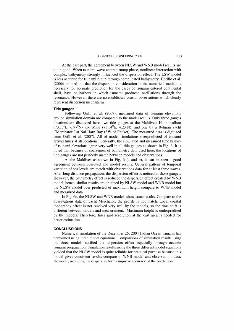
At the east part, the agreement between NLSW and WNB model results are

quite good. When tsunami wave entered runup phase, nonlinear interaction with

complex bathymetry strongly influenced the dispersion effect. The LSW model

is less accurate for tsunami runup through complicated bathymetry. Horillo et al.

(2006) pointed out that the dispersion consideration in the numerical models is

necessary for accurate prediction for the cases of tsunami entered continental

shelf, bays or harbors in which tsunami produced oscillations through the

resonance. However, there are no established coastal observations which clearly

represent dispersion mechanism.

Tide gauges

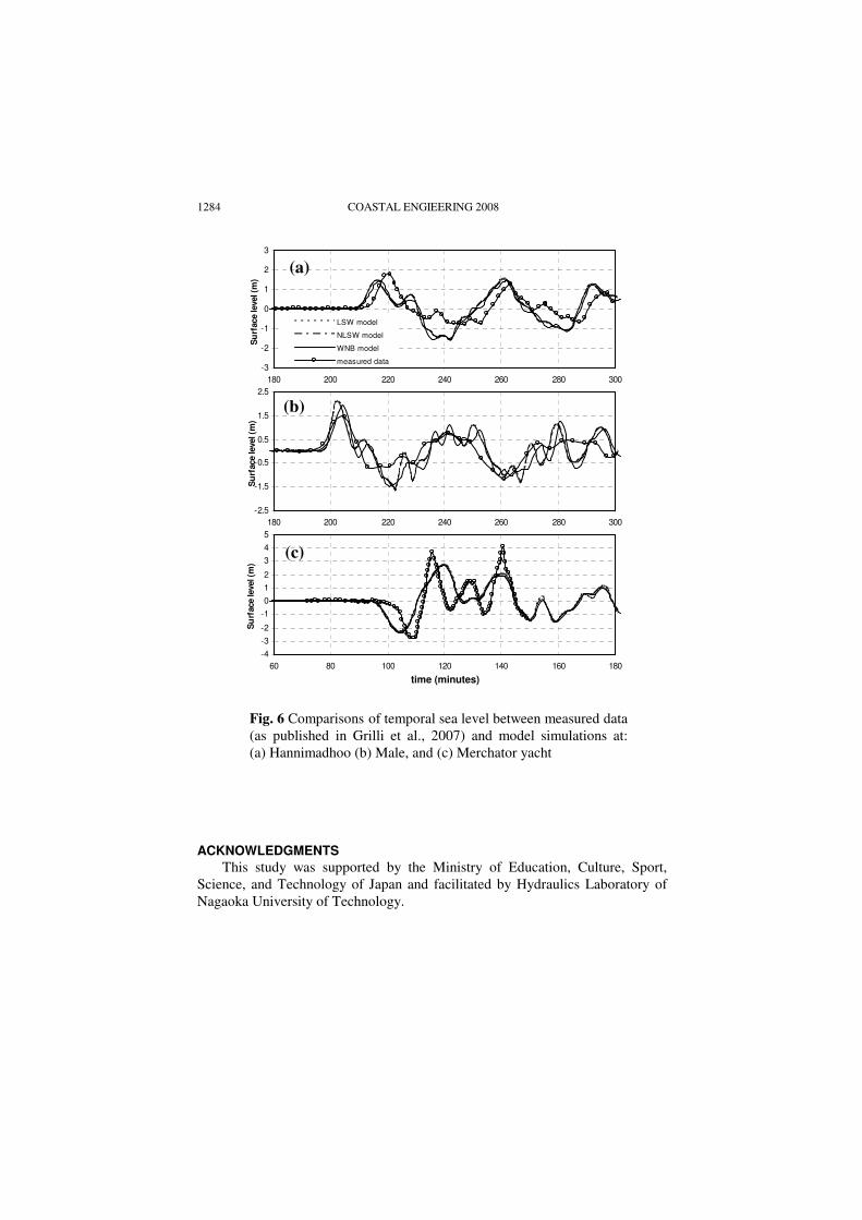
Following Grilli et al. (2007), measured data of tsunami elevations

around simulation domain are compared to the model results. Only three gauges

locations are discussed here, two tide gauges at the Maldives: Hannimadhoo

(73.170E, 6.77

0N) and Male (73.54

0E, 4.23

0N), and one by a Belgian yacht

‘’Merchator’’ at Nai Harn Bay (SW of Phuket). The measured data is digitized

from Grilli et al. (2007). All of model simulations overpredicted of tsunami

arrival times at all locations. Generally, the simulated and measured time history

of tsunami elevations agree very well in all tide gauges as shown in Fig. 6. It is

noted that because of coarseness of bathymetry data used here, the locations of

tide gauges are not perfectly match between models and observations.

At the Maldives as shown in Fig. 6 (a and b), it can be seen a good

agreement between observed and model results. General pattern of temporal

variation of sea levels are match with observations data for at least three waves.

After long distance propagation, the dispersion effect is noticed at those gauges.

However, the bathymetry effect is reduced the dispersion effect created by WNB

model, hence, similar results are obtained by NLSW model and WNB model but

the NLSW model over predicted of maximum height compare to WNB model

and measured data.

In Fig. 6c, the NLSW and WNB models show same results. Compare to the

observations data of yacht Merchator, the profile is not match. Local coastal

topography effect is not resolved very well by the models, so the time shift is

different between models and measurement. Maximum height is underpredited

by the models. Therefore, finer grid resolution at the east area is needed for

better estimation.

CONCLUSSIONS

Numerical simulation of the December 26, 2004 Indian Ocean tsunami has

performed using three model equations. Comparisons of simulation results using

the three models notified the dispersion effect especially through oceanic

tsunami propagation. Simulation results using the three different model equations

yielded that the NLSW model is quite reliable for practical purpose because this

model gives consistent results compare to WNB model and observations data.

However, including the dispersive terms improve accuracy of the prediction.

1284 COASTAL ENGIEERING 2008

ACKNOWLEDGMENTS

This study was supported by the Ministry of Education, Culture, Sport,

Science, and Technology of Japan and facilitated by Hydraulics Laboratory of

Nagaoka University of Technology.

-3

-2

-1

0

1

2

3

180 200 220 240 260 280 300

Su

rface level (m

)

LSW model

NLSW model

WNB model

measured data

-2.5

-1.5

-0.5

0.5

1.5

2.5

180 200 220 240 260 280 300

Su

rface level (m

)

-4

-3

-2

-1

0

1

2

3

4

5

60 80 100 120 140 160 180

Su

rface level (m

)

time (minutes)

Fig. 6 Comparisons of temporal sea level between measured data

(as published in Grilli et al., 2007) and model simulations at:

(a) Hannimadhoo (b) Male, and (c) Merchator yacht

(a)

(b)

(c)

COASTAL ENGINEERING 2008 1285

APPENDIX

The model equations are written in the following form to make convenient

for applying high order time stepping

[ ]

[ ]

1

1

1

( , , ) ( ) ,

( , , ) ( ) ,

( , , ) ( )

tt

t t

t t

E u v E h

U F u v F v

V G u v G u

η = η +

= η +

= η +

(A-1)

( ) ( ) ( )

( )

3 2

1 2

3 2

1 2

( , , ) ( ) ( ) ( )

( ) ( ) ( )

xx xy xx xyx y x

xy yy xy yyy

E u v Hu Hv a h u v a h hu hv

a h u v a h hu hv

η = − − − + + +

− + + +

(A-2)

( ) ( )2 2

1 2 2( ) x yx y

E h h a h h a h h= − − − (A-3)

2( , , ) ( )

x x y b brF u v g u vu F Fη = − η − − − + (A-4)

1 1 2 2( ) ( )

xy xy xF v h b hv b hv b h = + + (A-5)

2( , , ) ( )

y x y b brG u v g uv v G Gη = − η − − − + (A-6)

1 1 2 2( ) ( )

xy xy yG u h b hu b hu b h = + + (A-7)

2 2

1 2 1 2( ) ; ( )

xx xx yy yyU u b h u b h hu V v b h v b h hv= + + = + + (A-8)

where H h= + η is total water depth. Subscript t denotes partial derivative with

respect to time, while subscript x and y denote spatial derivatives in the x and y

direction, respectively. Variables 1 2 1 2, , ,a a b b are defined as

2 21 1 1 1

1 2 1 22 6 2 2, , , / 0.531a a b b z h= β − = β + = β = β = = −ɶ (A-9)

for WNB model equations and 1 2 1 2

0a a b b= = = = for NLSW or LSW model

equations.

Adam-Bashforth-Moulton scheme are used here as of Wei and Kirby (1995) and

written as

( )1 1 1 2 1 2

, , , , , 1 , 1 , 1 ,1223 16 5 2( ) 3( ) ( )

n n n n n n n nti j i j i j i j i j i j i j i j

+ + − − − −∆Ω = Ω + Φ − Φ + Φ + Φ − Φ + Φ (A-10)

for predictor step and

( )1 1 1 1 2 1

, , , , , , 1 , 1 ,249 19 5 ( ) ( )

n n n n n n n nti j i j i j i j i j i j i j i j

+ + + − − +∆Ω = Ω + Φ + Φ − Φ + Φ + Φ − Φ (A-11)

for corrector step, where ( , , )U VΩ = η , ( , , )E F GΦ = and 1 1 1 1( , , )E F GΦ =

The values of u and v at time level (n+1) could be obtained by solving (A-8)

using double sweep algorithm to solve tridiagonal matrix system.

1286 COASTAL ENGIEERING 2008

REFERENCES

Chen, Q., Kirby, J.T., Dalrymple, R.A., Kennedy, A.B., and Chawla, A. 2000.

Boussinesq modeling of wave transformation, breaking, and runup. II: 2D,

J. Waterway, Port, Coast, and Ocean Engineering, ASCE, 126(1), 48-56.

Grilli, S. T., Ioualalen, M., Asavanant, J., Shi, F., Kirby, J.T., and Watts, P.

(2007). Source Constraints and Model Simulation of the December 26,

2004, Indian Ocean Tsunami. J. Waterway, Port, Coast, and Ocean

Engineering, ASCE, 133(6), 414 – 428.

Horillo, J., Kowalik, Z., and Shigihara, Y. 2006. Wave dispersion study in The

Indian Ocean Tsunami of December 26, 2004, Science of Tsunami Hazards,

25(1), 42-63.

Kennedy, A.B., Chen, Q., Kirby, J.T., and Dalrymple, R.A. 2000. Boussinesq

modeling of wave transformation, breaking, and runup. I: 1D, J. Waterway,

Port, Coast, and Ocean Engineering, ASCE, 126(1), 39-47.

Kowalik, Z. 2003. Basic relations between tsunamis and calculation and their

physics-II, Science of Tsunami Hazards, 21(3), 154-173.

Kowalik, Z., Knight, W., Logan, T., and Whitmore, P. 2005. Numerical

modeling of the global tsunami: Indonesia Tsunami of 26 December 2004,

Science of Tsunami Hazards, 23(1), 40-56.

Lynett, P., and Liu, P.L.-F. 2002. A numerical study of submarine landslide

generated waves and runup, Proc. R. Society London, 458, 2885-2910.

Nwogu, O. 1993. Alternative form of Boussinesq equations for nearshor wave

propagation, J. Waterway, Port, Coast, and Ocean Engineering, ASCE,

119(6), 618-638.

Okada, Y. 1985. Surface deformation due to shear and tensile faults in a half-

space, Bulletin of the Seismological Society of America, 75(4), 1135-1154.

Watts, P., Ioualalen, M., GRilli, S., Shi, F., and Kirby, J.T. 2005. Numerical

simulation of the December 26, 2004 Indian Ocean tsunami using high-

order Boussinesq model, Fifth Int. Symp. WAVES 2005, Madrid Spain, 10pp

Wei, G. and Kirby, J.T. 1995. Time-dependent numerical code for extended

Boussinesq equations, J. Waterway, Port, Coast, and Ocean Engineering,

ASCE, 121(5), 251-261.

Wei, G., Kirby, J. T., Grilli, S. T., and Subramanya, R. 1995. A fully nonlinear

Boussinesq model for surface waves. Part 1. Highly nonlinear unsteady

waves, J. Fluid Mechanic, 294, 71-92.

COASTAL ENGINEERING 2008 1287

KEYWORDS – ICCE 2008

NUMERICAL STUDY OF DISPERSION AND NONLINEARITY EFFECTS

ON TSUNAMI PROPAGATION

Authors: Alwafi Pujiraharjo and Tokuzo Hosoyamada

Abstract number: 1090

Boussinesq equations

Dispersive effect

Indian Ocean Tsunami

Nonlinear

Tsunami generation

Tsunami propagation