Embed Size (px)
Citation preview

University of VermontScholarWorks @ UVM
Graduate College Dissertations and Theses Dissertations and Theses
2012
Numerical Study of Disperse MonopropellantMicroslug Formation at a Cross JunctionRyan McDevitUniversity of Vermont
Follow this and additional works at: https://scholarworks.uvm.edu/graddis
This Thesis is brought to you for free and open access by the Dissertations and Theses at ScholarWorks @ UVM. It has been accepted for inclusion inGraduate College Dissertations and Theses by an authorized administrator of ScholarWorks @ UVM. For more information, please [email protected].
Recommended CitationMcDevit, Ryan, "Numerical Study of Disperse Monopropellant Microslug Formation at a Cross Junction" (2012). Graduate CollegeDissertations and Theses. 152.https://scholarworks.uvm.edu/graddis/152
NUMERICAL STUDY OF DISPERSE MONOPROPELLANT MICROSLUGFORMATION AT A CROSS JUNCTION
A Thesis Presented
by
M. Ryan McDevitt
to
The Faculty of the Graduate College
of
The University of Vermont
In Partial Fullfillment of the Requirementsfor the Degree of Master of Science
Specializing in Mechanical Engineering
October, 2011
Abstract
Two immiscible fluids converging at microchannel cross-junction results in the for-mation of periodic, dispersed microslugs. This microslug formation phenomenon hasbeen proposed as the basis for a fuel injection system in a novel, discrete mono-propellant microthruster design for use in next-generation nanosatellites. Previousexperimental work has demonstrated the ability to repeatably generate fuel slugs withcharacteristics commensurate with the intended application. In this work, numericalmodeling and simulation are used to further study this problem, and identify thesensitivity of the slug characteristics to key material properties including surface ten-sion, contact angle and fuel viscosity. These concerns are of practical concern for thisapplication due to the potential for thermal variations and/or fluid contaminationduring typical operation. For each of these properties, regions exist where the slugcharacteristics are essentially insensitive to property variations. Future microthrustersystem designs should target and incorporate these stable flow regions in their baselineoperating conditions to maximize robustness of operation.

Acknowledgements
First, and foremost, I would like to thank Professor Darren Hitt, whose support,
guidance and patience made this work possible.
Special thanks to JW McCabe, who laid the groundwork for this thesis.
Funding for this work has been provided by NASA under Cooperative Agreement
#NNX09A059
ii

Table of Contents
Acknowledgments . . . . . . . . . . . . . . . . . . . . . . . . . . . . . . . . . . . . . . . . . . . . . . . . . . . ii
List of Tables. . . . . . . . . . . . . . . . . . . . . . . . . . . . . . . . . . . . . . . . . . . . . . . . . . . . . . . . vi
List of Figures. . . . . . . . . . . . . . . . . . . . . . . . . . . . . . . . . . . . . . . . . . . . . . . . . . . . . . . vii
Chapter 1 Introduction. . . . . . . . . . . . . . . . . . . . . . . . . . . . . . . . . . . . . . . . . . . . . 1
1.1 Micro-Scale Propulsion . . . . . . . . . . . . . . . . . . . . . . . . . . 4
1.2 MEMS-Based Thrusters . . . . . . . . . . . . . . . . . . . . . . . . . 6
1.2.1 MEMS-Based FEEP Thruster . . . . . . . . . . . . . . . . . . 7
1.2.2 MEMS-Based Colloid Thruster . . . . . . . . . . . . . . . . . 8
1.2.3 Solid Propellant Digital Microthruster . . . . . . . . . . . . . 10
1.2.4 MEMS-Based Cold Gas Thruster . . . . . . . . . . . . . . . . 11
1.2.5 Vaporizing Liquid Microthruster . . . . . . . . . . . . . . . . . 13
1.2.6 MEMS-Based Monopropellant Thruster . . . . . . . . . . . . . 14
1.3 Flow Actuation & Microvalves . . . . . . . . . . . . . . . . . . . . . . 17
Chapter 2 A Discrete Monopropellant Microthruster Concept . . . . . . 22
2.1 Concept Overview . . . . . . . . . . . . . . . . . . . . . . . . . . . . 24
2.2 Discrete Microslug Formation . . . . . . . . . . . . . . . . . . . . . . 26
iii
2.3 Preliminary Considerations . . . . . . . . . . . . . . . . . . . . . . . . 29
Chapter 3 Computational Methodology . . . . . . . . . . . . . . . . . . . . . . . . . . . . 31
3.1 Governing Equations . . . . . . . . . . . . . . . . . . . . . . . . . . . 31
3.1.1 Boundary Conditions . . . . . . . . . . . . . . . . . . . . . . . 34
3.2 Computational Implementation . . . . . . . . . . . . . . . . . . . . . 37
3.2.1 Baseline Material Properties . . . . . . . . . . . . . . . . . . . 37
3.2.2 2D vs. 3D Results . . . . . . . . . . . . . . . . . . . . . . . . 37
3.2.3 Computational Domain & Grid Resolution Studies . . . . . . 39
3.3 Experimental Setup . . . . . . . . . . . . . . . . . . . . . . . . . . . . 42
3.4 Data Analysis . . . . . . . . . . . . . . . . . . . . . . . . . . . . . . . 44
3.4.1 Data Collection . . . . . . . . . . . . . . . . . . . . . . . . . . 46
3.4.2 Slug Length Analysis . . . . . . . . . . . . . . . . . . . . . . . 47
3.4.3 Slug Volume Analysis . . . . . . . . . . . . . . . . . . . . . . . 48
3.4.4 List of Studies . . . . . . . . . . . . . . . . . . . . . . . . . . . 51
Chapter 4 Results . . . . . . . . . . . . . . . . . . . . . . . . . . . . . . . . . . . . . . . . . . . . . . . . . . 54
4.1 Qualitative Comparison with Experimental Data . . . . . . . . . . . . 54
4.2 Impact of Surface Tension Variation . . . . . . . . . . . . . . . . . . . 55
4.3 Impact of Contact Angle Variation . . . . . . . . . . . . . . . . . . . 61
4.4 Impact of Thermally-Induced
Viscosity Variation . . . . . . . . . . . . . . . . . . . . . . . . . . . . 63
4.5 Effective Impulse and Thrust . . . . . . . . . . . . . . . . . . . . . . 67
Chapter 5 Conclusions . . . . . . . . . . . . . . . . . . . . . . . . . . . . . . . . . . . . . . . . . . . . . 77
5.1 Future Work . . . . . . . . . . . . . . . . . . . . . . . . . . . . . . . . 78
References . . . . . . . . . . . . . . . . . . . . . . . . . . . . . . . . . . . . . . . . . . . . . . . . . . . . . . . . . . 80
iv

Appendix A . . . . . . . . . . . . . . . . . . . . . . . . . . . . . . . . . . . . . . . . . . . . . . . . . . . . . . . . 85
v
List of Tables
1.1 Parameters used in evaluation of microvalves . . . . . . . . . . . . . . 18
1.2 Recent microvalve initiatives. Abbreviations are as follows, Style: NC
= Normally Closed; Type: TP = Thermo-Pneumatic, BM = Bimorph,
SMA = Shape Memory Alloy, ES = Electrostatic, PZ=Piezoelectric. . 20
3.1 Properties of H2O2 and N2 at STP . . . . . . . . . . . . . . . . . . . 37
3.2 Comparison of the initial slug in the “short” and “long” computational
domains . . . . . . . . . . . . . . . . . . . . . . . . . . . . . . . . . . 40
3.3 Comparison of relevant material properties used in the simulations and
experiments . . . . . . . . . . . . . . . . . . . . . . . . . . . . . . . . 43
3.4 Comparison of the different slug volume calculation methods . . . . . 50
3.5 Surface Tension Coefficient Studies . . . . . . . . . . . . . . . . . . . 52
3.6 Contact Angle Studies . . . . . . . . . . . . . . . . . . . . . . . . . . 52
3.7 Fuel Viscosity Studies . . . . . . . . . . . . . . . . . . . . . . . . . . 53
vi
List of Figures
1.1 Conceptual illustration of the ESA/NASA LISA mission. Courtesy of
NASA JPL website (http://lisa.jpl.nasa.gov) . . . . . . . . . . . . . . 5
1.2 Illustration of the Field Emission Electric Propulsion (FEEP) concept.
Liquid metal propellant in the reservoir enters the slit via capillary
action and exits at the accelerator. . . . . . . . . . . . . . . . . . . . 8
1.3 Schematic representation of the FEEP thruster showing the etch and
deposition required. Designed by Fleron [10] . . . . . . . . . . . . . . 9
1.4 Basic operation of a colloid thruster using the electrospray technique.
Reproduced from Nabity [12] . . . . . . . . . . . . . . . . . . . . . . . 9
1.5 Schematic of device built by Xiong et al.. The sandwich fabrication
simplifies the etch geometry for each layer. Each layer is stacked and
bonded to complete the thruster. Xiong et al. quotes several etch
technologies including a KOH chemical etch and an inductively-coupled
plasma etch. Reproduced from Xiong [13] . . . . . . . . . . . . . . . . 10
1.6 Schematic of the sandwich constructed microthruster chip. The single-
shot thrust concept was one popular among the aerospace community
for its simple design and precise impulse bit. Reproduced from Lewis [14] 12
vii
1.7 Digital solid propellant microthruster designed and built by TRW and
Aerospace Corporation. Courtesy of TRW. Reproduced from NASA
GSFC Electric Eng. Div. website . . . . . . . . . . . . . . . . . . . . 13
1.8 Picture of the cold gas thruster presented by Fuqua et al. in 1999.
The device is a sandwich design consisting of a propellant feed line,
valve, plenum and nozzle. The device works properly during thruster
operation. However leaks through the valve, which is common among
cold gas thrusters, is an issue. Reproduced from Fuqua [15] . . . . . . 14
1.9 VLM integrated with solenoid valve and Pyrex thermal standoff. Re-
produced from Blandino et al. [17] . . . . . . . . . . . . . . . . . . . . 15
1.10 VLM test model dimensions (top view, drawing not to scale): A=618
µm, B= 62 µm, C=709 µm, D=7.8 mm, E=1.1 mm, and depth =
300µm. Reproduced from Blandino et al. [17] . . . . . . . . . . . . . 16
1.11 Illustration of the operation of a hydrogen peroxide thruster. Repro-
duced from Hitt et al. [9] . . . . . . . . . . . . . . . . . . . . . . . . . 16
1.12 A digital photograph of the completed MEMS diamond pillar mi-
crothruster. A top view is shown, with the inlet at the bottom and the
nozzle at the top of the figure. To provide a reference length scale, a
US penny is included in the background. Reproduced from Hitt et al. [9] 17
2.1 Image of the NASA/Goddard Space Flight Center prototype micro
thruster. . . . . . . . . . . . . . . . . . . . . . . . . . . . . . . . . . . 23
viii
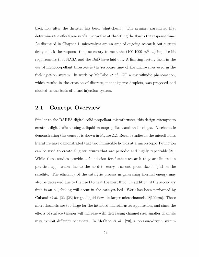
2.2 A schematic diagram depicting the envisioned operation of the discrete
monopropellant thruster. Flows of a monopropellant and a gaseous in-
ert fluid converge at a 90◦ junction. The result is a periodic sequence
of discrete monopropellant slugs, which propagate down the channel
where they are chemically-decomposed in a catalytic bed. The ener-
getic gases of decomposition in combination with the inert gas are then
expanded in a converging/diverging supersonic nozzle to produce the
target impulse for that slug. . . . . . . . . . . . . . . . . . . . . . . . 25
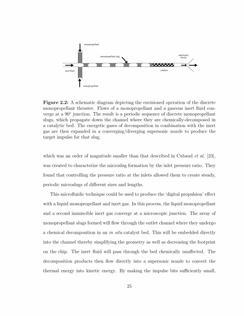
2.3 An image of slug formation in a microchannel with the pressure at all
inlets equal to 30 psi. . . . . . . . . . . . . . . . . . . . . . . . . . . . 26
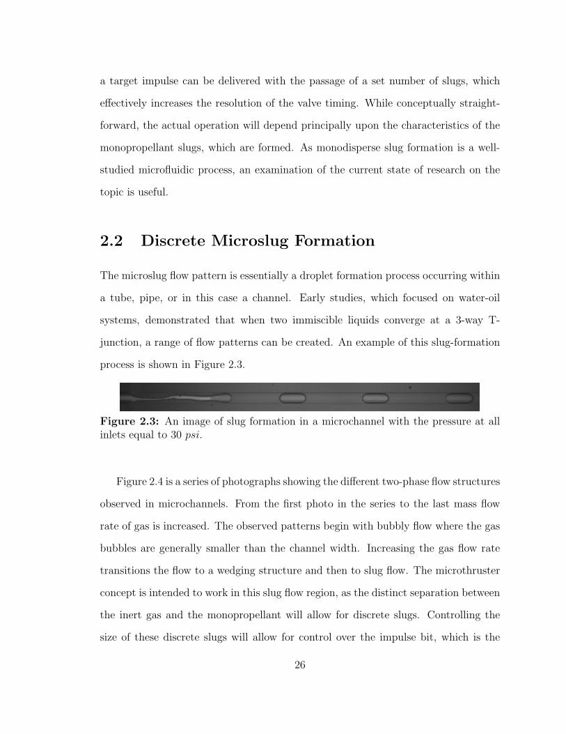
2.4 Photo of two phase flow structures in microchannels studied by Cubaud
and Ho [22]. . . . . . . . . . . . . . . . . . . . . . . . . . . . . . . . . 27
2.5 Flow pattern map for a gasliquid flow in microchannels studied by
Cubaud and Ho [23]. . . . . . . . . . . . . . . . . . . . . . . . . . . . 28
3.1 Definition of the contact angle, θ within COMSOL. . . . . . . . . . . 36
3.2 Plots of the 3D simulation of the baseline case. . . . . . . . . . . . . . 38
3.3 Comparison of the surface plots of the level set function for the 2D and
3D cases. . . . . . . . . . . . . . . . . . . . . . . . . . . . . . . . . . . 39
3.4 (a) The geometry of the microchannel used for flow visualization ex-
periments. (b) The geometry of the computational domain that corre-
sponds to the junction outlined in (a). . . . . . . . . . . . . . . . . . 40
3.5 Plot of the slug length as a function of time for various grids. . . . . . 42
ix
3.6 a) Schematic of the microchannel chip layout. The insert shows the
four-way junction. b) Schematic of the microchannel cross section.
The width of the mask line is 10 µm. The top piece of glass has the
access holes and the bottom piece has the etched pattern. The two are
fused together in the final steps of the manufacturing process. . . . . 44
3.7 Layout schematic for the pressure supply system with locations of fil-
ters and measurement devices. . . . . . . . . . . . . . . . . . . . . . . 45
3.8 Sample surface plot of the baseline simulation. The liquid is repre-
sented in black, and the gas is represented in white. . . . . . . . . . . 46
3.9 Block diagram showing the general process of the MATLAB script.
The outcomes are highlighted in orange. . . . . . . . . . . . . . . . . 46
4.1 A qualitative comparison of the experimental and numerical results. 1)
The upstream attachment mechanism. 2) The downstream detachment
mechanism. 3) The large, channel filling bubbles. . . . . . . . . . . . 55
4.2 Sample of results generated by varying the surface tension coefficient
with ∆V = 0 over an equivalent time period, with the simulated mono-
propellant in blue. . . . . . . . . . . . . . . . . . . . . . . . . . . . . 56
4.3 A plot of slug length vs. surface tension coefficient for fixed ∆V = 0
and Vliquid = .4ms
. . . . . . . . . . . . . . . . . . . . . . . . . . . . . 57
4.4 A plot of slug length vs. ∆V for three different surface tension coeffi-
cients. This plot highlights the similarity of the results. . . . . . . . . 58
4.5 A plot of slug formation frequency vs. surface tension coefficient, for
∆V = 0ms
. There is a clear transition between .06 Nm
and .07 Nm
. . . . 59
4.6 A plot of slug formation frequency vs ∆V for three different surface
tension coefficients. This plot highlights the similarity of the results. . 60
x
4.7 The plot of slug length as a function of contact angle. There is a clear
transition between 155 and 160 degrees, which corresponds to a change
in pinch-off mechanism. . . . . . . . . . . . . . . . . . . . . . . . . . . 62
4.8 Contour plots showing the change in detachment location that leads
to change in microslug length. . . . . . . . . . . . . . . . . . . . . . . 63
4.9 A plot of slug length vs. ∆V for three different contact angles. This
plot highlight the similarity of the results for these contact angles. . . 64
4.10 A plot of slug length vs. fuel viscosity for ∆V = 0. At 1.8 cP, the
system transitions to annular flow, with no slugs being made. . . . . . 66
4.11 A plot of slug formation frequency vs. fuel viscosity for ∆V = 0. As
the system transitions to annular flow at 18 cP, the formation frequency
drops to 0. . . . . . . . . . . . . . . . . . . . . . . . . . . . . . . . . . 67
4.12 A plot of slug length vs. ∆V for two different fuel viscosities. There is
a clear similarity between the two solutions. . . . . . . . . . . . . . . 68
4.13 A plot of slug formation frequency vs. ∆V for two different fuel vis-
cosities. There is a clear similarity between the two solutions. . . . . 69
4.14 A plot of the total thrust vs. surface tension coefficient for ∆V = 0ms
.
The baseline thrust is plotted in green. . . . . . . . . . . . . . . . . . 71
4.15 A plot of the impulse per slug vs. surface tension coefficient for ∆V = 0ms
. 72
4.16 A plot of total thrust vs. contact angle for ∆V = 0ms
. The baseline
thrust is plotted in green. . . . . . . . . . . . . . . . . . . . . . . . . 73
4.17 A plot of impulse per slug vs. contact angle for ∆V = 0ms
. . . . . . . 74
4.18 A plot of total thrust vs. viscosity for ∆V = 0ms
. The baseline thrust
is plotted in green. . . . . . . . . . . . . . . . . . . . . . . . . . . . . 75
4.19 A plot of impulse per slug vs. viscosity for ∆V = 0ms
. . . . . . . . . . 76
xi
Chapter 1
Introduction
Recent initiatives in the satellite technology sector have shown the benefits of minia-
turized satellites and point to the needs of future missions. Driven by the need
to lower costs, lower post launch maintenance and increase reliability, miniaturized
satellites are increasingly being used for a wide range of applications by academia,
government and industry. One of the major initiatives to meet these goals is the focus
on a group of miniaturized satellites (> 10kg) called nanosatellites [1]. Nanosatellites,
or “nanosats” allow for new science and communication missions by using satellite
designs that would not be feasible, either from a design standpoint or due to budget
constraints, with typical satellite architectures. Early efforts in nanosat design include
the CubeSat program, which is a set of specifications for a 10x10x10 cm satellite that
weighs 1 kg and is intended primarily for academic use. This system, designed by
CalPoly and Stanford in 1999 [2] was created to be low cost (> $40, 000) by using
off-the-shelf components. Due to the small volume and mass limitations, CubeSats
generally do not contain any thrusters on-board for precision station-keeping maneu-
vers. This limits their ability to perform precision communications or surveillance
missions, as both of these require maintaining position and orientation for success.
1
As mission designers focus on replacing larger satellites with nanosats, or fleets of
nanosats, developing appropriately-sized thrusters that are capable of Current NASA
and DoD goals for future nanosats require thrusters which are capable of thrust levels
and impulse bits on the order of (10-100 µN) and (100-1000 µN · s) respectively [3].
To date no MEMS-based propulsion systems have been implemented in nanosatel-
lites, however some have been flight tested for demonstration and experimental pur-
poses. Most recently, the Electric MIcrothruster Test in Space (EMITS) was one such
demonstration for flight testing a small-scale FEEP thruster capable of < 1µN thrust
levels [4]. This device was launched aboard a Space Shuttle mission as part of the
NASA Hitchhiker program using a Get-Away-Special (GAS) canister. FEEP, or Field
Emission Electric Propulsion, is of great interest to the small spacecraft community
because of its simplicity and thrust ranges. Typical thrust ranges are between 1 and
100 µN for drag free control and as high as 1 mN for larger crafts, however the device
itself is not a MEMS-based thruster but rather a MEMS-hybrid. The PRISMA pro-
gram, which launched in early 2010 and is currently ongoing, is positioned to be the
first flight demonstration of MEMS-based propulsion in a formation-flying test. The
propulsion system for this mission, designed by NanoSpace, is a MEMS-based cold gas
thruster with thrust output in the micro- to milli- Newton range. These propulsion
system tests are the next step toward realizing some of the next generation science
missions.
When speaking of micropropulsion systems, there is a distinction between micro-
level thrusters, and micro-scale thrusters. While nanosats will require micro-scale
propulsion systems, owing to their small size, there are missions currently in devel-
opment that will use large (> 20 kg) satellites that require micro-level thrust as
part of their mission design. One such mission that requires micro-level thrust is
the NASA/ESA LISA mission, or Laser Interferometer Space Antenna. LISA, which
2
is currently scheduled for an early 2012 launch, will study gravity waves, how they
propagate and the sources that emit them, first postulated in Einsteins Theory of
General Relativity. An illustration of the proposed design is shown in Figure 1.1.
The antenna is made up of three identical drag-free1 spacecraft arranged in a trian-
gle and placed at Lagrange points, the center of which orbits the Sun at 1 AU, and
located 20◦ behind the earth. Each arm of the triangle is approximately five million
kilometers and is roughly equilateral (due to these large spacings one spacecraft has
an orbit that intersects with the orbital path of Venus). The individual spacecraft will
each require special heliocentric orbits to minimize the change in distance between
them. The drag-free portion of the spacecraft is two test masses made of 75% gold
and 25% platinum, highly polished to function as a mirror and in the shape of a cube.
The test masses must maintain a central position in the craft to within a picometer.
Laser light is emitted from one spacecraft toward each of the others and reflected off
of the test mass to a sensor attached to the craft. The craft that receives the first
beam emits an in-phase beam at that precise moment back to the original craft. This
is done because of the decay in amplitude of the laser light over this large distance. In
a sense the second craft serves as a laser light repeater. However, since the spacecraft
are all identical either one may act as the initiator and therefore can conduct mea-
surements concurrently. This provides redundancy to the system as well as adding
to the accuracy in measurement [5]. In addition to the complexities of orbital flight
dynamics associated with these requirements each spacecraft must be capable of min-
imizing orbital perturbations and attitude changes due to non-gravitational forces
while keeping the test masses at the center of the spacecraft. Both radiation pressure
1A drag-free satellite is constructed of a freely floating object housed within an enclosed body
or craft. The craft is typically chasing the freely floating object by firing thrusters mounted on its
exterior attempting to keep the object in the center of the craft.
3
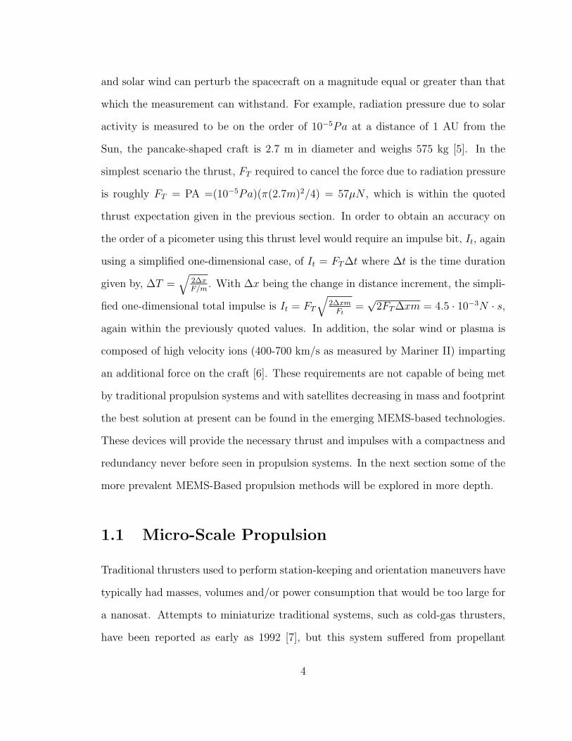
and solar wind can perturb the spacecraft on a magnitude equal or greater than that
which the measurement can withstand. For example, radiation pressure due to solar
activity is measured to be on the order of 10−5Pa at a distance of 1 AU from the
Sun, the pancake-shaped craft is 2.7 m in diameter and weighs 575 kg [5]. In the
simplest scenario the thrust, FT required to cancel the force due to radiation pressure
is roughly FT = PA =(10−5Pa)(π(2.7m)2/4) = 57µN , which is within the quoted
thrust expectation given in the previous section. In order to obtain an accuracy on
the order of a picometer using this thrust level would require an impulse bit, It, again
using a simplified one-dimensional case, of It = FT∆t where ∆t is the time duration
given by, ∆T =√
2∆xF/m
. With ∆x being the change in distance increment, the simpli-
fied one-dimensional total impulse is It = FT
√2∆xmFt
=√
2FT∆xm = 4.5 · 10−3N · s,
again within the previously quoted values. In addition, the solar wind or plasma is
composed of high velocity ions (400-700 km/s as measured by Mariner II) imparting
an additional force on the craft [6]. These requirements are not capable of being met
by traditional propulsion systems and with satellites decreasing in mass and footprint
the best solution at present can be found in the emerging MEMS-based technologies.
These devices will provide the necessary thrust and impulses with a compactness and
redundancy never before seen in propulsion systems. In the next section some of the
more prevalent MEMS-Based propulsion methods will be explored in more depth.
1.1 Micro-Scale Propulsion
Traditional thrusters used to perform station-keeping and orientation maneuvers have
typically had masses, volumes and/or power consumption that would be too large for
a nanosat. Attempts to miniaturize traditional systems, such as cold-gas thrusters,
have been reported as early as 1992 [7], but this system suffered from propellant
4
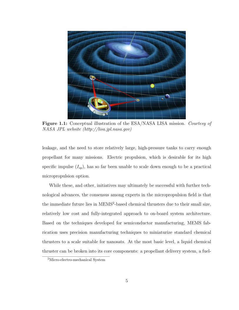
Figure 1.1: Conceptual illustration of the ESA/NASA LISA mission. Courtesy ofNASA JPL website (http://lisa.jpl.nasa.gov)
leakage, and the need to store relatively large, high-pressure tanks to carry enough
propellant for many missions. Electric propulsion, which is desirable for its high
specific impulse (Isp), has so far been unable to scale down enough to be a practical
micropropulsion option.
While these, and other, initiatives may ultimately be successful with further tech-
nological advances, the consensus among experts in the micropropulsion field is that
the immediate future lies in MEMS2-based chemical thrusters due to their small size,
relatively low cost and fully-integrated approach to on-board system architecture.
Based on the techniques developed for semiconductor manufacturing, MEMS fab-
rication uses precision manufacturing techniques to miniaturize standard chemical
thrusters to a scale suitable for nanosats. At the most basic level, a liquid chemical
thruster can be broken into its core components: a propellant delivery system, a fuel-
2Micro-electro-mechanical System
5
injection system, a combustion chamber and a supersonic nozzle. Depending on the
specific type of thruster these subsystems may be simple or quite complex. The goal
of the MEMS approach is to shrink each of these components down and integrate
them into a single system.
1.2 MEMS-Based Thrusters
As MEMS manufacturing is based on semiconductor fabrication techniques, it is un-
surprising that they have followed a similar miniaturization path. Advances in mate-
rials science and processing techniques have allowed for increasingly complex systems
that are orders of magnitude smaller than the first systems. Of particular interest
for nanosat designers is the incorporation of MEMS technology into micropropulsion
systems [1]. Most of these MEMS-based thrusters are miniaturizations of existing
systems.
Most current MEMS manufacturing is done on silicon wafers, or ‘chips’, due to its
semiconductor heritage. This imposes limits on the use of other materials that may be
desirable, but thin film deposition techniques (silicon oxide, silicon nitride, etc.) have
been developed that allow for the inclusion of other materials to be integrated during
the manufacturing process. Additionally, new nanoscale manufacturing techniques,
like nanorods made of various materials, show promise as catalysts in propellant
decomposition in monopropellant thrusters.
The focus on MEMS-based micropropulsion initiatives began in the 1990’s, spear-
headed by research at the Aerospace Corporation and NASA’s Jet Propulsion Lab-
oratory (JPL) [1]. These early efforts were focused on electric propulsion, including
resistojets, ion propulsion and FEEP thrusters. Later in the decade, focus turned
to liquid thrusters such as the Vaporizing Liquid Microthruster (VLM) at JPL [8]
6
and more recently a MEMS-based monopropellant thruster using hydrogen perox-
ide decomposition [9]. In the following sections, these early efforts at MEMS-based
thrusters will be discussed to highlight the challenges that exist for each technology.
1.2.1 MEMS-Based FEEP Thruster
Development of a MEMS-based FEEP thruster is an area of ongoing research; while
there have been several FEEP thrusters used aboard spacecraft, such as the EMITS
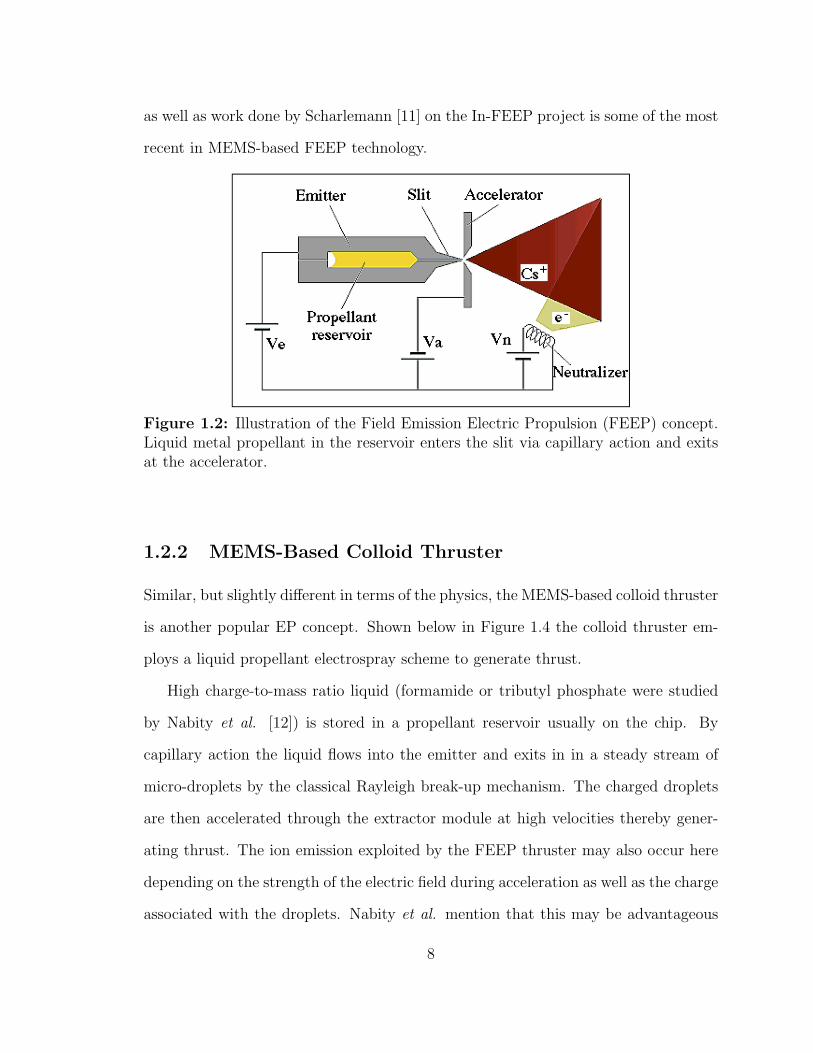
program, miniaturization has proven challenging. The underlying concept of a non-
MEMS FEEP thruster is highlighted in Figure 1.2. A liquid metal, typically cesium,
rubidium or indium is used as a propellant. The propellant is stored within the
emitter module consisting of two metallic plates sandwiched together but electrically
isolated from one another. The propellant flow enters the slit module by capillary
action and the free surface at the slit exit is exposed to a strong electric field, on the
order of 109V/m. The free surface undergoes a local instability due to the electrostatic
forces and surface effects, resulting in Taylor cones. At the tip of these cones atoms
spontaneously ionize at which point the accelerator electrode forces the ionized atoms
to eject from the device. There is an electron build-up in the propellant storage
reservoir that must be neutralized by electron emission into the ion jet.
To achieve this on the MEMS scale capillary tubes are etched using DRIE 3 into
the handle wafer on an SOI 4 substrate. The slit is within the oxide layer and the
accelerator and neutralizer modules are within the device layer of the SOI. In Figure
1.3 the cross section of a single device is shown. In the work done by Fleron and Hales
[10] a matrix of these capillaries are etched into the SOI substrate and are sectioned
into individually addressable areas to vary the thrust level. The work done by Fleron
3Deep Reactive Ion Etching4Silicon-on-Insulator
7
as well as work done by Scharlemann [11] on the In-FEEP project is some of the most
recent in MEMS-based FEEP technology.
Figure 1.2: Illustration of the Field Emission Electric Propulsion (FEEP) concept.Liquid metal propellant in the reservoir enters the slit via capillary action and exitsat the accelerator.
1.2.2 MEMS-Based Colloid Thruster
Similar, but slightly different in terms of the physics, the MEMS-based colloid thruster
is another popular EP concept. Shown below in Figure 1.4 the colloid thruster em-
ploys a liquid propellant electrospray scheme to generate thrust.
High charge-to-mass ratio liquid (formamide or tributyl phosphate were studied
by Nabity et al. [12]) is stored in a propellant reservoir usually on the chip. By
capillary action the liquid flows into the emitter and exits in in a steady stream of
micro-droplets by the classical Rayleigh break-up mechanism. The charged droplets
are then accelerated through the extractor module at high velocities thereby gener-
ating thrust. The ion emission exploited by the FEEP thruster may also occur here
depending on the strength of the electric field during acceleration as well as the charge
associated with the droplets. Nabity et al. mention that this may be advantageous
8
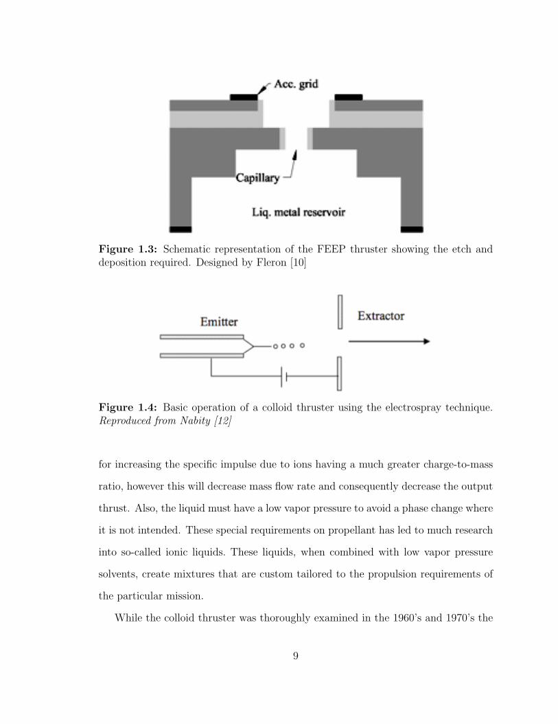
Figure 1.3: Schematic representation of the FEEP thruster showing the etch anddeposition required. Designed by Fleron [10]
Figure 1.4: Basic operation of a colloid thruster using the electrospray technique.Reproduced from Nabity [12]
for increasing the specific impulse due to ions having a much greater charge-to-mass
ratio, however this will decrease mass flow rate and consequently decrease the output
thrust. Also, the liquid must have a low vapor pressure to avoid a phase change where
it is not intended. These special requirements on propellant has led to much research
into so-called ionic liquids. These liquids, when combined with low vapor pressure
solvents, create mixtures that are custom tailored to the propulsion requirements of
the particular mission.
While the colloid thruster was thoroughly examined in the 1960’s and 1970’s the
9
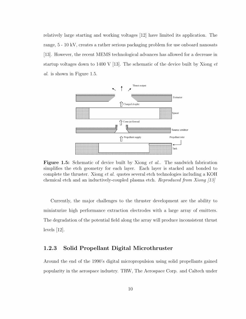
relatively large starting and working voltages [12] have limited its application. The
range, 5 - 10 kV, creates a rather serious packaging problem for use onboard nanosats
[13]. However, the recent MEMS technological advances has allowed for a decrease in
startup voltages down to 1400 V [13]. The schematic of the device built by Xiong et
al. is shown in Figure 1.5.
Figure 1.5: Schematic of device built by Xiong et al.. The sandwich fabricationsimplifies the etch geometry for each layer. Each layer is stacked and bonded tocomplete the thruster. Xiong et al. quotes several etch technologies including a KOHchemical etch and an inductively-coupled plasma etch. Reproduced from Xiong [13]
Currently, the major challenges to the thruster development are the ability to
miniaturize high performance extraction electrodes with a large array of emitters.
The degradation of the potential field along the array will produce inconsistent thrust
levels [12].
1.2.3 Solid Propellant Digital Microthruster
Around the end of the 1990’s digital micropropulsion using solid propellants gained
popularity in the aerospace industry. TRW, The Aerospace Corp. and Caltech under
10
Lewis et al. [14] began the Digital Propulsion project in the hopes of offering new
orbit and station-keeping operations at a fraction of the current costs. The schematic
of the device designed by Lewis et al. is shown in Figure 1.6.
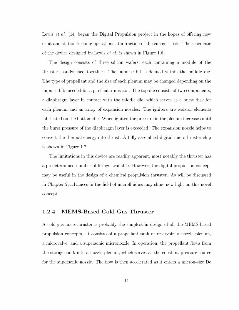
The design consists of three silicon wafers, each containing a module of the
thruster, sandwiched together. The impulse bit is defined within the middle die.
The type of propellant and the size of each plenum may be changed depending on the
impulse bits needed for a particular mission. The top die consists of two components,
a diaphragm layer in contact with the middle die, which serves as a burst disk for
each plenum and an array of expansion nozzles. The igniters are resistor elements
fabricated on the bottom die. When ignited the pressure in the plenum increases until
the burst pressure of the diaphragm layer is exceeded. The expansion nozzle helps to
convert the thermal energy into thrust. A fully assembled digital microthruster chip
is shown in Figure 1.7.
The limitations in this device are readily apparent, most notably the thruster has
a predetermined number of firings available. However, the digital propulsion concept
may be useful in the design of a chemical propulsion thruster. As will be discussed
in Chapter 2, advances in the field of microfluidics may shine new light on this novel
concept.
1.2.4 MEMS-Based Cold Gas Thruster
A cold gas microthruster is probably the simplest in design of all the MEMS-based
propulsion concepts. It consists of a propellant tank or reservoir, a nozzle plenum,
a microvalve, and a supersonic micronozzle. In operation, the propellant flows from
the storage tank into a nozzle plenum, which serves as the constant pressure source
for the supersonic nozzle. The flow is then accelerated as it enters a micron-size De
11
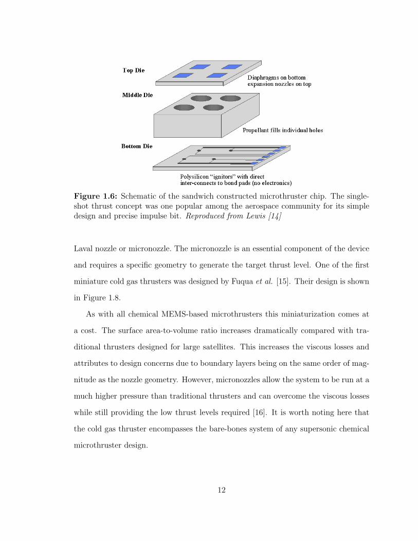
Figure 1.6: Schematic of the sandwich constructed microthruster chip. The single-shot thrust concept was one popular among the aerospace community for its simpledesign and precise impulse bit. Reproduced from Lewis [14]
Laval nozzle or micronozzle. The micronozzle is an essential component of the device
and requires a specific geometry to generate the target thrust level. One of the first
miniature cold gas thrusters was designed by Fuqua et al. [15]. Their design is shown
in Figure 1.8.
As with all chemical MEMS-based microthrusters this miniaturization comes at
a cost. The surface area-to-volume ratio increases dramatically compared with tra-
ditional thrusters designed for large satellites. This increases the viscous losses and
attributes to design concerns due to boundary layers being on the same order of mag-
nitude as the nozzle geometry. However, micronozzles allow the system to be run at a
much higher pressure than traditional thrusters and can overcome the viscous losses
while still providing the low thrust levels required [16]. It is worth noting here that
the cold gas thruster encompasses the bare-bones system of any supersonic chemical
microthruster design.
12
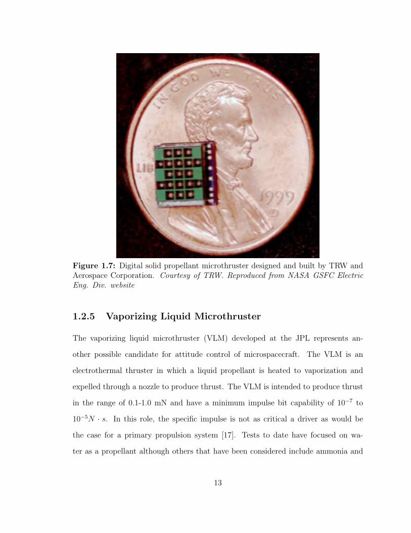
Figure 1.7: Digital solid propellant microthruster designed and built by TRW andAerospace Corporation. Courtesy of TRW. Reproduced from NASA GSFC ElectricEng. Div. website
1.2.5 Vaporizing Liquid Microthruster
The vaporizing liquid microthruster (VLM) developed at the JPL represents an-
other possible candidate for attitude control of microspacecraft. The VLM is an
electrothermal thruster in which a liquid propellant is heated to vaporization and
expelled through a nozzle to produce thrust. The VLM is intended to produce thrust
in the range of 0.1-1.0 mN and have a minimum impulse bit capability of 10−7 to
10−5N · s. In this role, the specific impulse is not as critical a driver as would be
the case for a primary propulsion system [17]. Tests to date have focused on wa-
ter as a propellant although others that have been considered include ammonia and
13
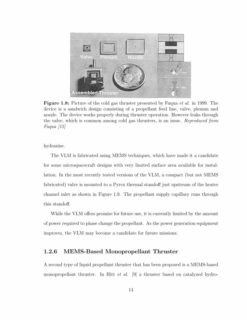
Figure 1.8: Picture of the cold gas thruster presented by Fuqua et al. in 1999. Thedevice is a sandwich design consisting of a propellant feed line, valve, plenum andnozzle. The device works properly during thruster operation. However leaks throughthe valve, which is common among cold gas thrusters, is an issue. Reproduced fromFuqua [15]
hydrazine.
The VLM is fabricated using MEMS techniques, which have made it a candidate
for some microspacecraft designs with very limited surface area available for instal-
lation. In the most recently tested versions of the VLM, a compact (but not MEMS
fabricated) valve is mounted to a Pyrex thermal standoff just upstream of the heater
channel inlet as shown in Figure 1.9. The propellant supply capillary runs through
this standoff.
While the VLM offers promise for future use, it is currently limited by the amount
of power required to phase change the propellant. As the power generation equipment
improves, the VLM may become a candidate for future missions.
1.2.6 MEMS-Based Monopropellant Thruster
A second type of liquid propellant thruster that has been proposed is a MEMS-based
monopropellant thruster. In Hitt et al. [9] a thruster based on catalyzed hydro-
14
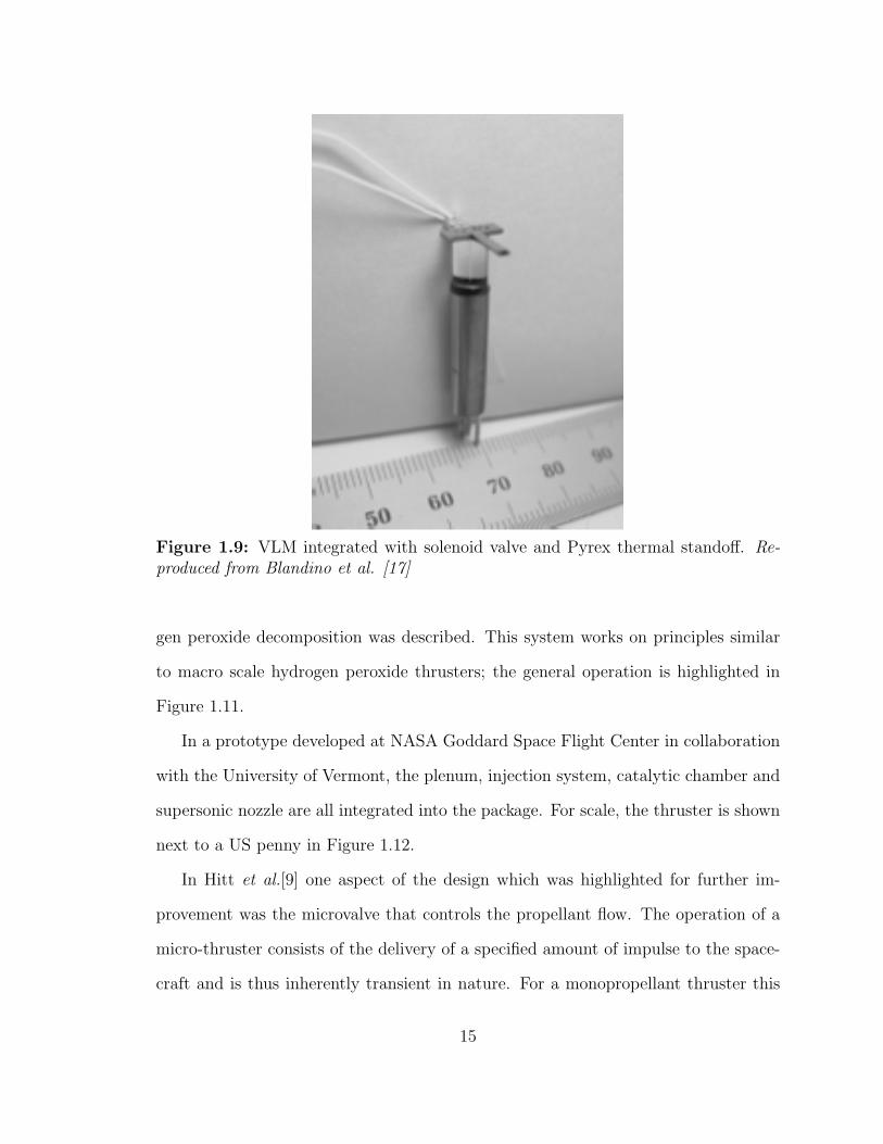
Figure 1.9: VLM integrated with solenoid valve and Pyrex thermal standoff. Re-produced from Blandino et al. [17]
gen peroxide decomposition was described. This system works on principles similar
to macro scale hydrogen peroxide thrusters; the general operation is highlighted in
Figure 1.11.
In a prototype developed at NASA Goddard Space Flight Center in collaboration
with the University of Vermont, the plenum, injection system, catalytic chamber and
supersonic nozzle are all integrated into the package. For scale, the thruster is shown
next to a US penny in Figure 1.12.
In Hitt et al.[9] one aspect of the design which was highlighted for further im-
provement was the microvalve that controls the propellant flow. The operation of a
micro-thruster consists of the delivery of a specified amount of impulse to the space-
craft and is thus inherently transient in nature. For a monopropellant thruster this
15
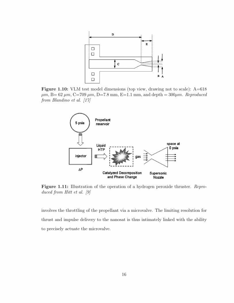
Figure 1.10: VLM test model dimensions (top view, drawing not to scale): A=618µm, B= 62 µm, C=709 µm, D=7.8 mm, E=1.1 mm, and depth = 300µm. Reproducedfrom Blandino et al. [17]
Figure 1.11: Illustration of the operation of a hydrogen peroxide thruster. Repro-duced from Hitt et al. [9]
involves the throttling of the propellant via a microvalve. The limiting resolution for
thrust and impulse delivery to the nanosat is thus intimately linked with the ability
to precisely actuate the microvalve.
16
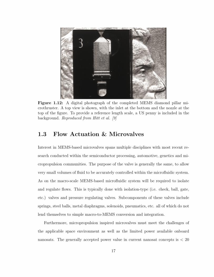
Figure 1.12: A digital photograph of the completed MEMS diamond pillar mi-crothruster. A top view is shown, with the inlet at the bottom and the nozzle at thetop of the figure. To provide a reference length scale, a US penny is included in thebackground. Reproduced from Hitt et al. [9]
1.3 Flow Actuation & Microvalves
Interest in MEMS-based microvalves spans multiple disciplines with most recent re-
search conducted within the semiconductor processing, automotive, genetics and mi-
cropropulsion communities. The purpose of the valve is generally the same, to allow
very small volumes of fluid to be accurately controlled within the microfluidic system.
As on the macro-scale MEMS-based microfluidic system will be required to isolate
and regulate flows. This is typically done with isolation-type (i.e. check, ball, gate,
etc.) valves and pressure regulating valves. Subcomponents of these valves include
springs, steel balls, metal diaphragms, solenoids, pneumatics, etc. all of which do not
lend themselves to simple macro-to-MEMS conversion and integration.
Furthermore, micropropulsion inspired microvalves must meet the challenges of
the applicable space environment as well as the limited power available onboard
nanosats. The generally accepted power value in current nanosat concepts is < 20
17
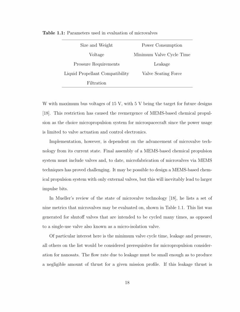
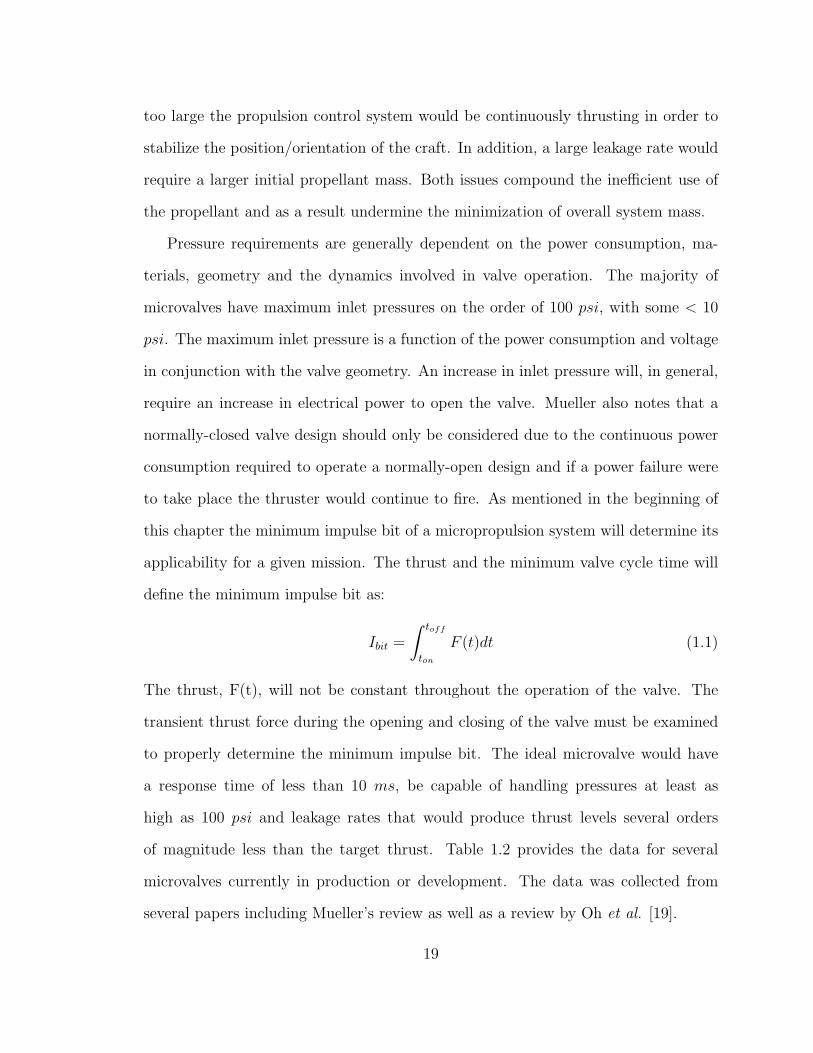
Table 1.1: Parameters used in evaluation of microvalves
Size and Weight Power Consumption
Voltage Minimum Valve Cycle Time
Pressure Requirements Leakage
Liquid Propellant Compatibility Valve Seating Force
Filtration
W with maximum bus voltages of 15 V, with 5 V being the target for future designs
[18]. This restriction has caused the reemergence of MEMS-based chemical propul-
sion as the choice micropropulsion system for microspacecraft since the power usage
is limited to valve actuation and control electronics.
Implementation, however, is dependent on the advancement of microvalve tech-
nology from its current state. Final assembly of a MEMS-based chemical propulsion
system must include valves and, to date, microfabrication of microvalves via MEMS
techniques has proved challenging. It may be possible to design a MEMS-based chem-
ical propulsion system with only external valves, but this will inevitably lead to larger
impulse bits.
In Mueller’s review of the state of microvalve technology [18], he lists a set of
nine metrics that microvalves may be evaluated on, shown in Table 1.1. This list was
generated for shutoff valves that are intended to be cycled many times, as opposed
to a single-use valve also known as a micro-isolation valve.
Of particular interest here is the minimum valve cycle time, leakage and pressure,
all others on the list would be considered prerequisites for micropropulsion consider-
ation for nanosats. The flow rate due to leakage must be small enough as to produce
a negligible amount of thrust for a given mission profile. If this leakage thrust is
18
too large the propulsion control system would be continuously thrusting in order to
stabilize the position/orientation of the craft. In addition, a large leakage rate would
require a larger initial propellant mass. Both issues compound the inefficient use of
the propellant and as a result undermine the minimization of overall system mass.
Pressure requirements are generally dependent on the power consumption, ma-
terials, geometry and the dynamics involved in valve operation. The majority of
microvalves have maximum inlet pressures on the order of 100 psi, with some < 10
psi. The maximum inlet pressure is a function of the power consumption and voltage
in conjunction with the valve geometry. An increase in inlet pressure will, in general,
require an increase in electrical power to open the valve. Mueller also notes that a
normally-closed valve design should only be considered due to the continuous power
consumption required to operate a normally-open design and if a power failure were
to take place the thruster would continue to fire. As mentioned in the beginning of
this chapter the minimum impulse bit of a micropropulsion system will determine its
applicability for a given mission. The thrust and the minimum valve cycle time will
define the minimum impulse bit as:
Ibit =
∫ toff
ton
F (t)dt (1.1)
The thrust, F(t), will not be constant throughout the operation of the valve. The
transient thrust force during the opening and closing of the valve must be examined
to properly determine the minimum impulse bit. The ideal microvalve would have
a response time of less than 10 ms, be capable of handling pressures at least as
high as 100 psi and leakage rates that would produce thrust levels several orders
of magnitude less than the target thrust. Table 1.2 provides the data for several
microvalves currently in production or development. The data was collected from
several papers including Mueller’s review as well as a review by Oh et al. [19].
19
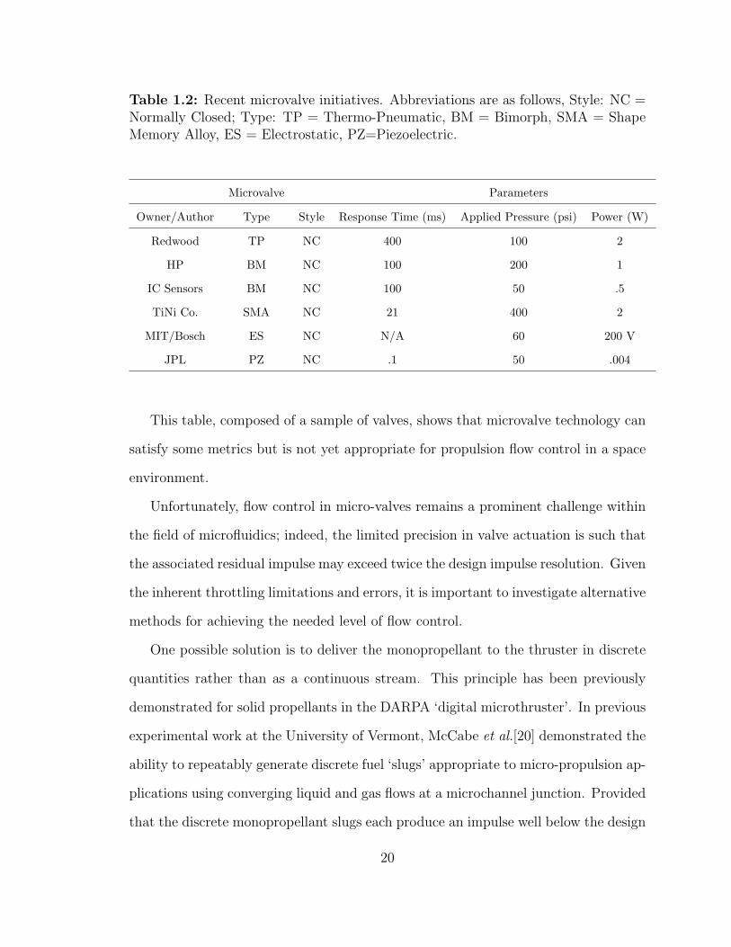
Table 1.2: Recent microvalve initiatives. Abbreviations are as follows, Style: NC =Normally Closed; Type: TP = Thermo-Pneumatic, BM = Bimorph, SMA = ShapeMemory Alloy, ES = Electrostatic, PZ=Piezoelectric.
Microvalve Parameters
Owner/Author Type Style Response Time (ms) Applied Pressure (psi) Power (W)
Redwood TP NC 400 100 2
HP BM NC 100 200 1
IC Sensors BM NC 100 50 .5
TiNi Co. SMA NC 21 400 2
MIT/Bosch ES NC N/A 60 200 V
JPL PZ NC .1 50 .004
This table, composed of a sample of valves, shows that microvalve technology can
satisfy some metrics but is not yet appropriate for propulsion flow control in a space
environment.
Unfortunately, flow control in micro-valves remains a prominent challenge within
the field of microfluidics; indeed, the limited precision in valve actuation is such that
the associated residual impulse may exceed twice the design impulse resolution. Given
the inherent throttling limitations and errors, it is important to investigate alternative
methods for achieving the needed level of flow control.
One possible solution is to deliver the monopropellant to the thruster in discrete
quantities rather than as a continuous stream. This principle has been previously
demonstrated for solid propellants in the DARPA ‘digital microthruster’. In previous
experimental work at the University of Vermont, McCabe et al.[20] demonstrated the
ability to repeatably generate discrete fuel ‘slugs’ appropriate to micro-propulsion ap-
plications using converging liquid and gas flows at a microchannel junction. Provided
that the discrete monopropellant slugs each produce an impulse well below the design
20
resolution, then a target level of impulse can be delivered to the nanosat by allowing
the passage of a finite number of slugs through the valve. In essence, the slug forma-
tion process represents a virtual self-valving mechanism which affords finer resolution
than a micro-valve for a continuous stream. McCabe et al.[20] demonstrated that
the slug size and frequency could be varied over a sizable range by carefully regulat-
ing inlet pressure conditions. Details of this micropropulsion concept are more fully
described in Chapter 2.
The present study is intended to both complement and extend the work of McCabe
et al. by developing a computational model capable of simulating the slug formation
process. This numerical capability is significant in that it allows for sensitivity studies
to be performed that are not easily accomplished experimentally: namely, the impact
of variations in key gas/liquid properties (surface tension, contact angle, viscosity)
that could potentially arise during an extended space mission due to fouling or thermal
variations within the propulsion system.
21
Chapter 2
A Discrete Monopropellant
Microthruster Concept
As highlighted in Chapter 1, monopropellant propulsion is an attractive scheme for
microthruster applications due to its advantages over other propulsion types:
• Lower power requirements than electro-thermal and electric propulsion devices
• Higher propellant density and higher specific impulse than cold-gas thrusters
• Greater thrust and impulse bit control than solid propellant systems
• Simpler to design and operate than bipropellant systems
Monopropellant thrusters typically rely upon a catalyzed chemical decomposition
of the liquid propellant as the source of energy. The chemical reaction, which is
exothermic, produces a high-energy gaseous product, which is accelerated through a
converging-diverging nozzle to generate thrust. Opening and closing the valve that
controls the flow of the liquid propellant can control the impulse bit of the system. The
first prototype monopropellant microthruster reported in literature was developed
22
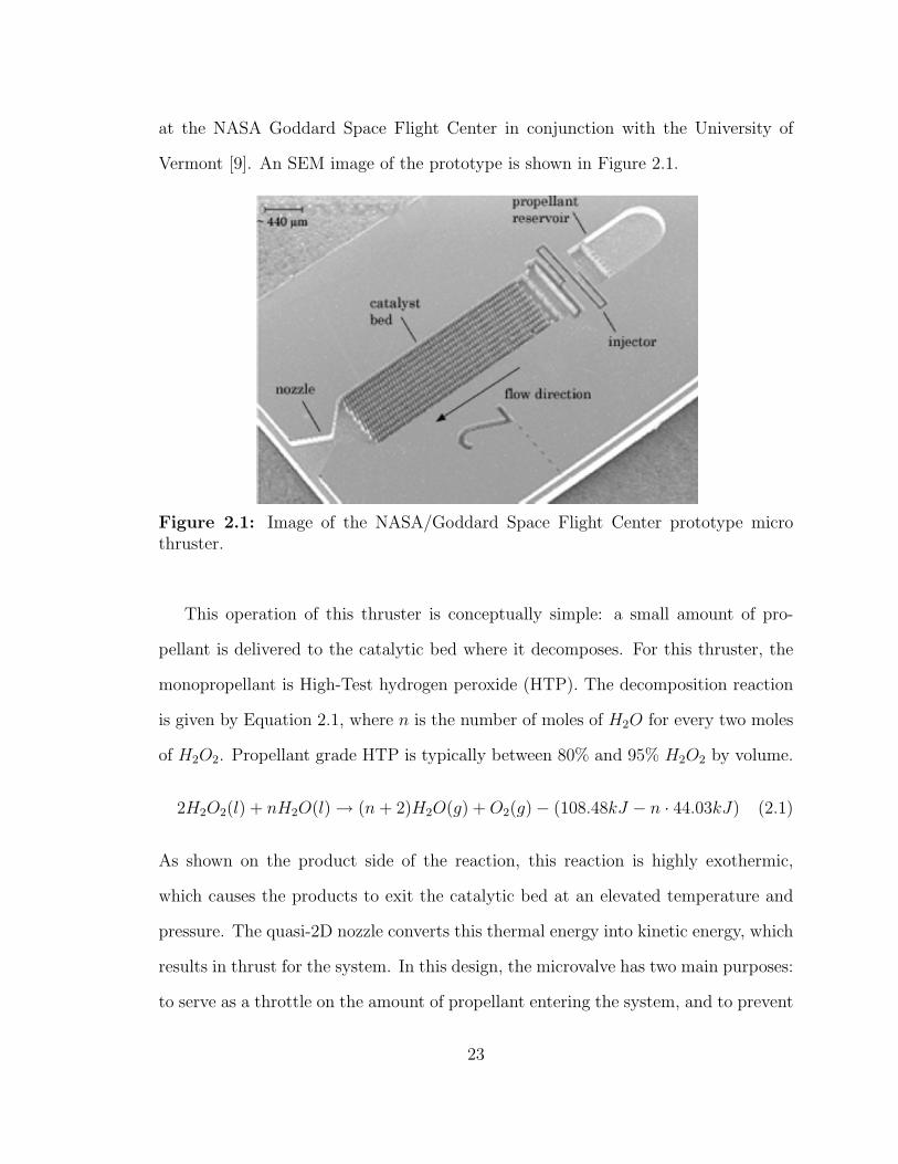
at the NASA Goddard Space Flight Center in conjunction with the University of
Vermont [9]. An SEM image of the prototype is shown in Figure 2.1.
Figure 2.1: Image of the NASA/Goddard Space Flight Center prototype microthruster.
This operation of this thruster is conceptually simple: a small amount of pro-
pellant is delivered to the catalytic bed where it decomposes. For this thruster, the
monopropellant is High-Test hydrogen peroxide (HTP). The decomposition reaction
is given by Equation 2.1, where n is the number of moles of H2O for every two moles
of H2O2. Propellant grade HTP is typically between 80% and 95% H2O2 by volume.
2H2O2(l) + nH2O(l)→ (n+ 2)H2O(g) +O2(g)− (108.48kJ − n · 44.03kJ) (2.1)
As shown on the product side of the reaction, this reaction is highly exothermic,
which causes the products to exit the catalytic bed at an elevated temperature and
pressure. The quasi-2D nozzle converts this thermal energy into kinetic energy, which
results in thrust for the system. In this design, the microvalve has two main purposes:
to serve as a throttle on the amount of propellant entering the system, and to prevent
23
back flow after the thruster has been “shut-down”. The primary parameter that
determines the effectiveness of a microvalve at throttling the flow is the response time.
As discussed in Chapter 1, microvalves are an area of ongoing research but current
designs lack the response time necessary to meet the (100-1000 µN · s) impulse-bit
requirements that NASA and the DoD have laid out. A limiting factor, then, in the
use of monopropellant thrusters is the response time of the microvalves used in the
fuel-injection system. In work by McCabe et al. [20] a microfluidic phenomenon,
which results in the creation of discrete, monodisperse droplets, was proposed and
studied as the basis of a fuel-injection system.
2.1 Concept Overview
Similar to the DARPA digital solid propellant microthruster, this design attempts to
create a digital effect using a liquid monopropellant and an inert gas. A schematic
demonstrating this concept is shown in Figure 2.2. Recent studies in the microfluidics
literature have demonstrated that two immiscible liquids at a microscopic T-junction
can be used to create slug structures that are periodic and highly repeatable.[21].
While these studies provide a foundation for further research they are limited in
practical application due to the need to carry a second pressurized liquid on the
satellite. The efficiency of the catalytic process in generating thermal energy may
also be decreased due to the need to heat the inert fluid. In addition, if the secondary
fluid is an oil, fouling will occur in the catalyst bed. Work has been performed by
Cubaud et al. [22],[23] for gas-liquid flows in larger microchannels O[100µm]. These
microchannels are too large for the intended microthruster application, and since the
effects of surface tension will increase with decreasing channel size, smaller channels
may exhibit different behaviors. In McCabe et al. [20], a pressure-driven system
24
inert fluid
monopropellant
catalyst
supersonic nozzle
monopropellant
monopropellant slug
Figure 2.2: A schematic diagram depicting the envisioned operation of the discretemonopropellant thruster. Flows of a monopropellant and a gaseous inert fluid con-verge at a 90◦ junction. The result is a periodic sequence of discrete monopropellantslugs, which propagate down the channel where they are chemically-decomposed ina catalytic bed. The energetic gases of decomposition in combination with the inertgas are then expanded in a converging/diverging supersonic nozzle to produce thetarget impulse for that slug.
which was an order of magnitude smaller than that described in Cubaud et al. [23],
was created to characterize the microslug formation by the inlet pressure ratio. They
found that controlling the pressure ratio at the inlets allowed them to create steady,
periodic microslugs of different sizes and lengths.
This microfluidic technique could be used to produce the ‘digital propulsion’ effect
with a liquid monopropellant and inert gas. In this process, the liquid monopropellant
and a second immiscible inert gas converge at a microscopic junction. The array of
monopropellant slugs formed will flow through the outlet channel where they undergo
a chemical decomposition in an in situ catalyst bed. This will be embedded directly
into the channel thereby simplifying the geometry as well as decreasing the footprint
on the chip. The inert fluid will pass through the bed chemically unaffected. The
decomposition products then flow directly into a supersonic nozzle to convert the
thermal energy into kinetic energy. By making the impulse bits sufficiently small,
25
a target impulse can be delivered with the passage of a set number of slugs, which
effectively increases the resolution of the valve timing. While conceptually straight-
forward, the actual operation will depend principally upon the characteristics of the
monopropellant slugs, which are formed. As monodisperse slug formation is a well-
studied microfluidic process, an examination of the current state of research on the
topic is useful.
2.2 Discrete Microslug Formation
The microslug flow pattern is essentially a droplet formation process occurring within
a tube, pipe, or in this case a channel. Early studies, which focused on water-oil
systems, demonstrated that when two immiscible liquids converge at a 3-way T-
junction, a range of flow patterns can be created. An example of this slug-formation
process is shown in Figure 2.3.
Figure 2.3: An image of slug formation in a microchannel with the pressure at allinlets equal to 30 psi.
Figure 2.4 is a series of photographs showing the different two-phase flow structures
observed in microchannels. From the first photo in the series to the last mass flow
rate of gas is increased. The observed patterns begin with bubbly flow where the gas
bubbles are generally smaller than the channel width. Increasing the gas flow rate
transitions the flow to a wedging structure and then to slug flow. The microthruster
concept is intended to work in this slug flow region, as the distinct separation between
the inert gas and the monopropellant will allow for discrete slugs. Controlling the
size of these discrete slugs will allow for control over the impulse bit, which is the
26
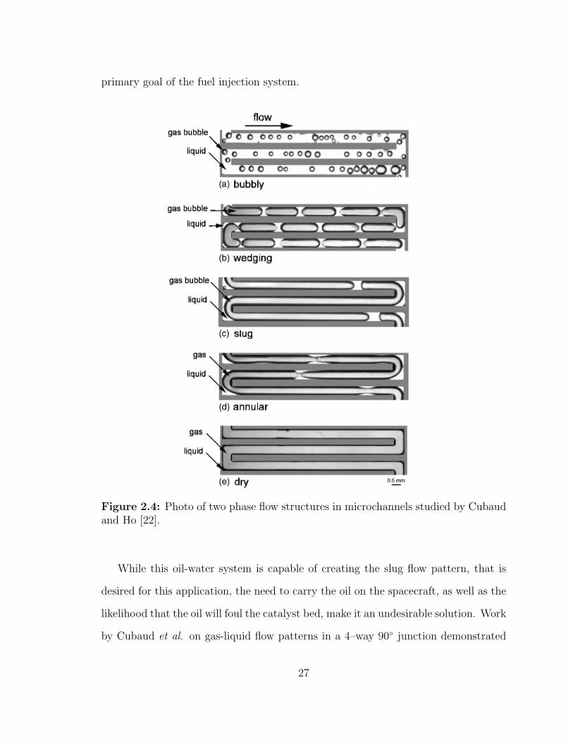
primary goal of the fuel injection system.
Figure 2.4: Photo of two phase flow structures in microchannels studied by Cubaudand Ho [22].
While this oil-water system is capable of creating the slug flow pattern, that is
desired for this application, the need to carry the oil on the spacecraft, as well as the
likelihood that the oil will foul the catalyst bed, make it an undesirable solution. Work
by Cubaud et al. on gas-liquid flow patterns in a 4–way 90◦ junction demonstrated
27
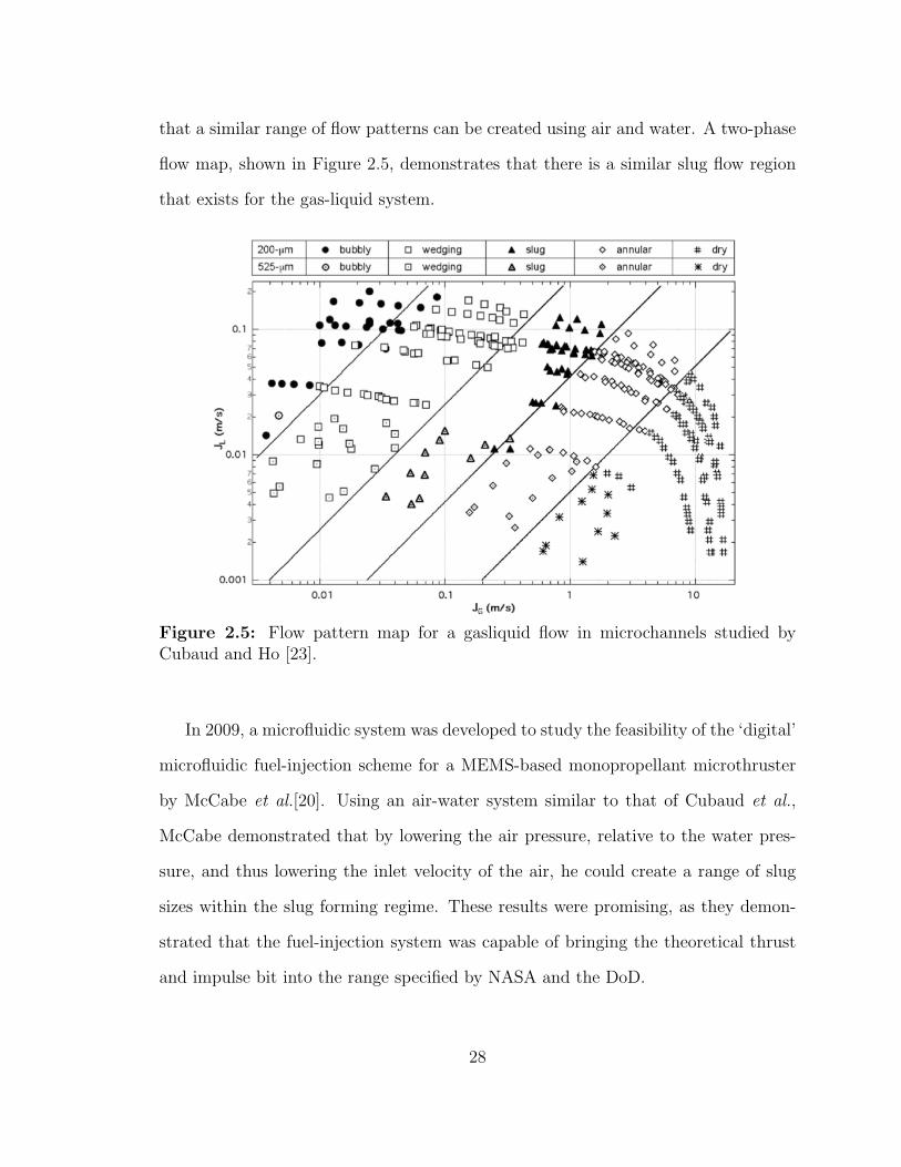
that a similar range of flow patterns can be created using air and water. A two-phase
flow map, shown in Figure 2.5, demonstrates that there is a similar slug flow region
that exists for the gas-liquid system.
Figure 2.5: Flow pattern map for a gasliquid flow in microchannels studied byCubaud and Ho [23].
In 2009, a microfluidic system was developed to study the feasibility of the ‘digital’
microfluidic fuel-injection scheme for a MEMS-based monopropellant microthruster
by McCabe et al.[20]. Using an air-water system similar to that of Cubaud et al.,
McCabe demonstrated that by lowering the air pressure, relative to the water pres-
sure, and thus lowering the inlet velocity of the air, he could create a range of slug
sizes within the slug forming regime. These results were promising, as they demon-
strated that the fuel-injection system was capable of bringing the theoretical thrust
and impulse bit into the range specified by NASA and the DoD.
28
2.3 Preliminary Considerations
In this work the slug flow pattern is dissected into two measurable quantities, namely
pinch-off frequency, f, and slug length, Ls. These two variables characterize the flow
and can be used to calculate both thrust and impulse bit. The pinch-off mechanism
is commonly understood to be the competition between pressure and surface tension,
as well as geometry and wall surface attributes such as contact angle. This process
results in the periodic formation of monodisperse micro-slugs. Given some geometry,
wall material(s) and fluid properties this can be written as:
f = g1(∆P, Pbase, σ, θ, µ,Dh, A) (2.2)
Ls = g2(∆P, Pbase, σ, θ, µ,Dh, A) (2.3)
where ∆P is the difference in gas and liquid inlet pressures, Pbase is the baseline inlet
pressure of the liquid, σ is the surface tension, θ is the contact angle, µ is the dynamic
viscosity of the liquid, Dh is the hydraulic diameter and A is the cross sectional area
of the microchannel. A change in the baseline pressure will have an effect on the
mean velocity of the flow. This term will account for the overall increase in mass flow
rate.
Of the terms in each of these groups, the first two (∆P and Pbase) are the pa-
rameters that will be controlled to specify the flow and the last two (Dh and A) are
geometric parameters that are specified by the system. In contrast, the surface ten-
sion, contact angle and viscosity terms may vary during operation. One of the main
conclusions of McCabe [24] was that surface tension effects dominate the slug forma-
tion process in smaller microchannels. Surface tension is a highly sensitive quantity
that can be significantly affected by the presence of contaminants and variations in
29

temperature. Viscosity, another temperature-dependent material property, and con-
tact angle, another property that could be affected by the presence of contaminants,
are also parameters of interest. The goal of this study is to use computer simulations
to examine the effects of these parameters on the slug formation process in the slug
forming regime that was studied experimentally by McCabe.
30
Chapter 3
Computational Methodology
In Chapter 2, the relevant parameters of interest for the multiphase flow were found
to be surface tension coefficient (σ), contact angle (θ) and dynamic viscosity of the
monopropellant (µ). The goal of this study was to determine the impact of each of
these parameters on the operation of the proposed microthruster. To achieve this
goal, computational fluid dynamics (CFD) simulations were performed, including
a formulation for tracking the interface between the two phases. In section 3.1, the
mathematical formulation of the transport equations will be presented, and in section
3.2 the computational methods used to solve these equations will be presented.
3.1 Governing Equations
In this study, the unsteady, incompressible Navier-Stokes equations were solved:
∇ · ui = 0 (3.1)
ρi∂ui
∂t+ ρi(ui · ∇)ui = ∇ · [−pI + µi(∇ui +∇uT
i )] + ~FST (3.2)
31
where u is the velocity of the fluid, ρ is the fluid density, p is the pressure, µ is the
dynamic viscosity, ~FST is the surface tension and the subscript i corresponds to the
appropriate phase. To track the movement of the interface between the two fluids,
the level set method was used. In the level set method, the discontinuity between
the two discrete phases is represented with the level set function φ, a continuous
function that represents the distance from the interface at all points in the domain.
The continuity of this function allows the system to handle large deformations of the
interface, including splitting into multiple functions. This function is commonly taken
to be a smoothed Heaviside function, with 0 representing one fluid and 1 representing
the other fluid. The φ = .5 isocontour then represents the interface between the two
phases [25]. As the flow field is calculated, the interface is advected by:
∂φ
∂t+ u · ∇φ = 0 (3.3)
The discontinuity in density (ρ) and viscosity (ν) are smoothed across the inter-
face using Eqns. 3.4 & 3.5:
ρ = ρ1 + (ρ2 − ρ1)φ (3.4)
ν = ν1 + (ν2 − ν1)φ (3.5)
where ρ1 and ν1 are the density and kinematic viscosity of the first fluid, and ρ2 and
ν2 are of the second fluid. The surface tension term, in Eqn 3.2, at a point ~x can be
calculated from:
~FST (~x) = σκ(~x)n(~x) (3.6)
where σ is the surface tension coefficient, n and κ are the unit normal and curvature
of the interface, respectively. In the level set method, n and κ can be calculated from
32
φ using:
n =∇φ|∇φ|
(3.7)
~κ = −∇ · ( ∇φ|∇φ|
) (3.8)
The surface tension equation can then be recast in terms of the surface tension coef-
ficient and the level set function:
~FST (~x) = σ(−∇ · ∇φ|∇φ|
)∇φ (3.9)
In this formulation, the surface tension represents a volume force that is spread across
the width of the interface. This new force is only equal to the surface tension in the
limit as the thickness of the interface goes to zero, which places an upper bound
on the maximum width of the interface. If the interface gets too small, however,
the discontinuity in density and viscosity cannot be properly smoothed, which yields
difficulties in computing the solution.
The general solution algorithm then, is to calculate the velocity of the flow using
the momentum transport equation. Next, this velocity is used to advect the level set
function, which modifies the shape of the interface. The curvature of the updated
interface is then used to calculate the surface tension force. This updated surface
tension force is then used at the next time step to solve the momentum equation.
One drawback of the level set method, in its standard formulation, is that it is
not mass conservative. At each successive time step, as the interface is moved it is
possible for it to move a greater distance than intended, which causes an inaccurate
reporting of the volume. [26]. In Olsson et al. a modified version of the level set was
developed to improve the mass conservation. In this method the movement of the
level set function (φ) is corrected by using a modified advection equation:
∂φ
∂t+ u · ∇φ = γ∇ · (ε∇φ− φ(1− φ)
∇φ|∇φ|
) (3.10)
33
where γ represents a re-initialization parameter that predicts where the interface has
moved to since the last time step and ε represents an estimated interface thickness.
For numerical stability, the minimum mesh size should be O[ε] and γ should be
roughly equivalent to the maximum velocity of the flow. When ε and γ are properly
selected, nearly perfect mass conservation is expected [27],[28]. The CFD program,
COMSOL Multiphysics was selected to perform the simulations. COMSOL is a finite
element based solver, which uses the mass-conservative formulation of the level set
method.
3.1.1 Boundary Conditions
The inlet boundary conditions for the computational model were selected to as closely
resemble previous experimental work as possible. In the flow visualization experi-
ments the gas and liquid phases are pressurized at 30 psi, and the slug lengths are
controlled by decreasing the air inlet pressure from this baseline. In the computa-
tional model, however, inlet velocity conditions were instead used as they proved to
be numerically stable over a wide range of inlet conditions. To find the necessary inlet
velocity to compare to the pressure range used in McCabe et al. [20] a hydrodynamic
analysis of the microfluidic channel was performed. This analysis is done assuming
that the flow is entirely propellant with no inert gas. What follows is the classical
Poiseuille flow given by:
∆P = Q ∗RHyd (3.11)
where ∆P is the upstream gage pressure, Q is the volumetric flow rate of propellant,
and Rhyd is the hydraulic resistance of the microchannel. This leaves two unknowns,
Q and Rhyd, that can be directly calculated using a few more relations. First, hy-
draulic resistance requires the knowledge of the microchannel geometry (length and
34
cross-sectional area) as well as the working fluids viscosity. The viscosity of HTP
is 1.245 cP at 20◦ C. The microchannel geometry will be shown in greater detail in
the following chapter, however for this analysis the length, L, is 90.28 mm and the
area, A, is 50 µm in width by 20 µm in depth. Because of large surface-to-volume
ratios in microchannels the simple hydraulic resistance calculation for non-circular
cross-sections was reexamined by Mortensen et al. [29]. They rewrite the hydraulic
resistance such that,
α =Rhyd
R∗hyd(3.12)
where R∗hyd = µL/A2 is a hydraulic resistance given by dimensional analysis and α
becomes a dimensionless geometrical correction factor. For this case, α is a function
of the compactness, C, which for a rectangular cross-section is given by Equation
3.13:
α(C) ≈ 22
7C − 65
3+O(|C − 18|2) (3.13)
Plugging all this in one finds a hydraulic resistance of 8.755 psiµl/min
(units were chosen
for simplicity in further calculations). These results compare well to tests run to
experimentally determine the hydraulic resistance by McCabe [24]. The analytical
value is comparable to the experimentally measured value of 8.25 psiµl/min
. Using this
hydraulic resistance, the estimated flow rate and thus the estimated inlet velocity can
be calculated. For the range of pressures calculated studied by McCabe, the inlet
velocity of the liquid phase is .38m/s. For the simulations inlet velocities of .4 ms
for all inlets were roughly similar to the 30 psi baseline, and decreasing the gas inlet
velocity by .05 ms
resulted in a drop of pressure of roughly .1 psi.
In addition to the inlets and outlets, the appropriate boundary conditions for
the walls must be determined. Typically, in CFD simulations, no-slip conditions are
imposed at the walls to account for the effects of friction. In the level set method,
35
a no-slip condition would be inaccurate, because it would prevent the interface from
moving along the walls. To account for this, there is a “wetted wall” boundary
condition implemented within COMSOL. This boundary condition uses a slip length,
which allows the interface to move along the wall, but adds a friction term to account
for the walls:
~Ffr = −µβ~u (3.14)
where µ is the dynamic viscosity of the liquid, ~u is the velocity of the fluids and β is
the slip length, which is typically equal to the width of a single finite element. The
contact angle is used to determine the shape of the interface at points where it comes
in contact with the walls. In COMSOL, the contact angle is defined according to the
diagram in Figure 3.1:
Figure 3.1: Definition of the contact angle, θ within COMSOL.
36
3.2 Computational Implementation
COMSOL Multiphysics was used to perform the CFD analysis on the system. The
following sections describe the selection of the baseline material properties, model
geometry and computational grid used for these studies.
3.2.1 Baseline Material Properties
As the goal of this study is to examine the behavior of the slug-generation process
over a range of parametric conditions, it was first necessary to establish a baseline
simulation, against which further parametric studies could be compared. The liquid
for these simulations was 90% hydrogen peroxide, while N2 was selected as the gas
for the simulations. Table 3.1 below shows the default values for the parameters of
interest.
Table 3.1: Properties of H2O2 and N2 at STP
Fluid H2O2 N2
Viscosity (cP) 1.245 .018
Surface Tension (dyncm
) 79.0 –
Contact Angle (Degrees) 180 –
3.2.2 2D vs. 3D Results
Due to the intense computational demands of simulating the flow in 3D, using a 2D
simulation was desirable for parametric studies. In Qian and Lawal [30], a strong con-
nection between the 2D and 3D simulations of micro-slug generation in microchannels
was found. To verify that a similar connection exists in this study, a 3D model of
37
the junction was simulated. An isosurface, and surface plot of these simulations are
presented in Figure 3.2 below:
(a) Isosurface plot of the .5 contour of the level set function in 3D
(b) Surface plot of the level set function in 3D
Figure 3.2: Plots of the 3D simulation of the baseline case.
Next, these results were compared against the 2D baseline model. A surface plot
of the 2D and 3D simulations of the baseline case are provided below:
The 2D models over-report the slug length compared to the 3D case by 11%; one
cause of this error was assumed to be the lack of friction that would occur in the
top and bottom of the channel. To account for this friction a body force term that
accounts for the friction of the liquid of the top and bottom of the channel was added.
This term, which is implemented in COMSOL as a correction for shallow channels, is:
38
(a) 2D Simulation
(b) 3D Simulation
Figure 3.3: Comparison of the surface plots of the level set function for the 2D and3D cases.
~FSC =12µ~u
ρh2(3.15)
where µ is the viscosity, ~u is the flow velocity, ρ is the density and h is the height of
the channel. Using this correction term resulted in slug lengths that are more in line
with the 3D simulations.
3.2.3 Computational Domain & Grid Resolution Studies
The geometry of the computational model was selected to matchup with the mi-
crochannel used in McCabe et al. [20] for comparison purposes. This microchannel,
shown in Figure 3.4, is 50 µm x 20 µm, with the distance from the liquid inlet ports
to the junction of 3 mm and the distance from the gas inlet port to the junction of
6 mm. To reduce the computational domain, the inlet lengths were truncated to 150
µm and 300 µm respectively. The resulting domain is shown in Figure 3.4b. To ac-
count for the affects along the length of the channel that is not simulated, a laminar
inflow boundary condition is implemented. In COMSOL, this boundary condition
calculates the pressure drop and velocity profile of the channel and uses that as the
39
inlet values for the simulation. The outlet channel, which contains the microslugs,
is truncated from 80 mm on the microchannel to 2200 µm in the simulation, with a
laminar outflow boundary condition used to account for the downstream effects that
are outside of the computational domain.
Figure 3.4: (a) The geometry of the microchannel used for flow visualization ex-periments. (b) The geometry of the computational domain that corresponds to thejunction outlined in (a).
To demonstrate that the results generated were independent of the downstream
portion of the system, that are not being directly simulated, a model with an increased
downstream domain (4500 µm) was also simulated. A comparison of the length of
the first slug in both the “short” and “long” downstream domain are presented in
Table 3.2, where the uncertainty is because the computational grid cannot be fully
resolved on a per pixel basis:
Table 3.2: Comparison of the initial slug in the “short” and “long” computationaldomains
Slug Length (µm) Standard Deviation
Short 139 4.63
Long 142 4.24
Percent Difference 2% 9%
The similarity between the two simulations illustrates that the laminar outflow
40
boundary condition is sufficient to account for the portion of the domain that is not
being explicitly simulated, with dramatically reduced overhead.
While using the short channel provides a drastic reduction in processing time
required, it does impose some limitations on the simulation. Specifically, the laminar
outflow boundary condition is unable to simulate the interface as it exits the domain.
For this reason, all simulations are limited in duration to the point where the first gas
bubble reaches the outlet of the domain. This occurs between .018 - .025 s depending
on the inlet boundary conditions. This is typically long enough to generate 10-20
slugs. In Section 3.4.2 analysis was performed to demonstrate that this is enough
slugs to use for statistical analysis.
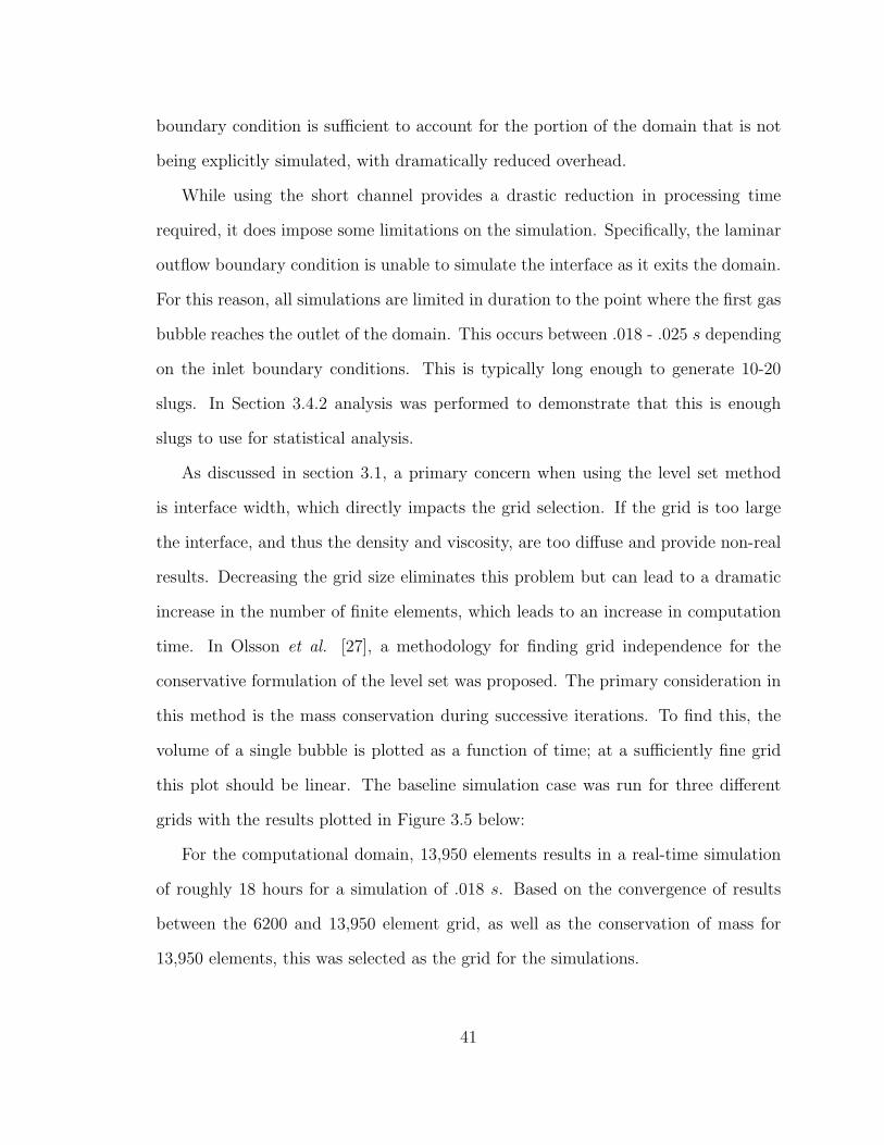
As discussed in section 3.1, a primary concern when using the level set method
is interface width, which directly impacts the grid selection. If the grid is too large
the interface, and thus the density and viscosity, are too diffuse and provide non-real
results. Decreasing the grid size eliminates this problem but can lead to a dramatic
increase in the number of finite elements, which leads to an increase in computation
time. In Olsson et al. [27], a methodology for finding grid independence for the
conservative formulation of the level set was proposed. The primary consideration in
this method is the mass conservation during successive iterations. To find this, the
volume of a single bubble is plotted as a function of time; at a sufficiently fine grid
this plot should be linear. The baseline simulation case was run for three different
grids with the results plotted in Figure 3.5 below:
For the computational domain, 13,950 elements results in a real-time simulation
of roughly 18 hours for a simulation of .018 s. Based on the convergence of results
between the 6200 and 13,950 element grid, as well as the conservation of mass for
13,950 elements, this was selected as the grid for the simulations.
41
Time (s)
Sem
i-Maj
or A
xis
(pix
els)
0.0005 0.001 0.0015 0.00235
40
45
50
55
60
65
70
751350 Elements6200 Elements13950 Elements
Figure 3.5: Plot of the slug length as a function of time for various grids.
3.3 Experimental Setup
To provide a baseline comparison for numerical simulations, a limited set of exper-
imental data was collected using the procedure developed by McCabe. [20] These
comparisons were used to confirm that the general results being created in the simu-
lations were in line with the experimental data.
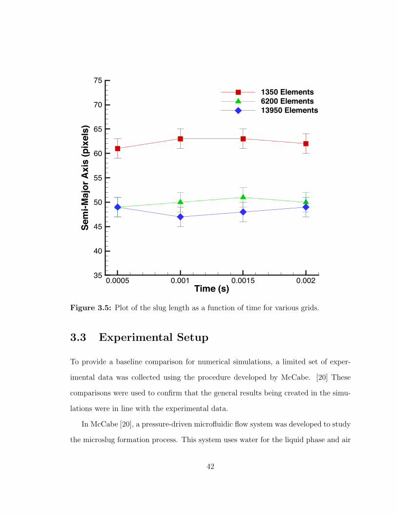
In McCabe [20], a pressure-driven microfluidic flow system was developed to study
the microslug formation process. This system uses water for the liquid phase and air
42
for the gas phase; these are selected for their accessibility and chemical similarity to
H2O2 and N2 respectively as shown in Table 3.3:
Table 3.3: Comparison of relevant material properties used in the simulations andexperiments
Fluid H2O2 H2O N2 Air
Viscosity (cP) 1.245 1.0016 .0178 .0183
Surface Tension (dyncm
) 79.0 72.7 – –
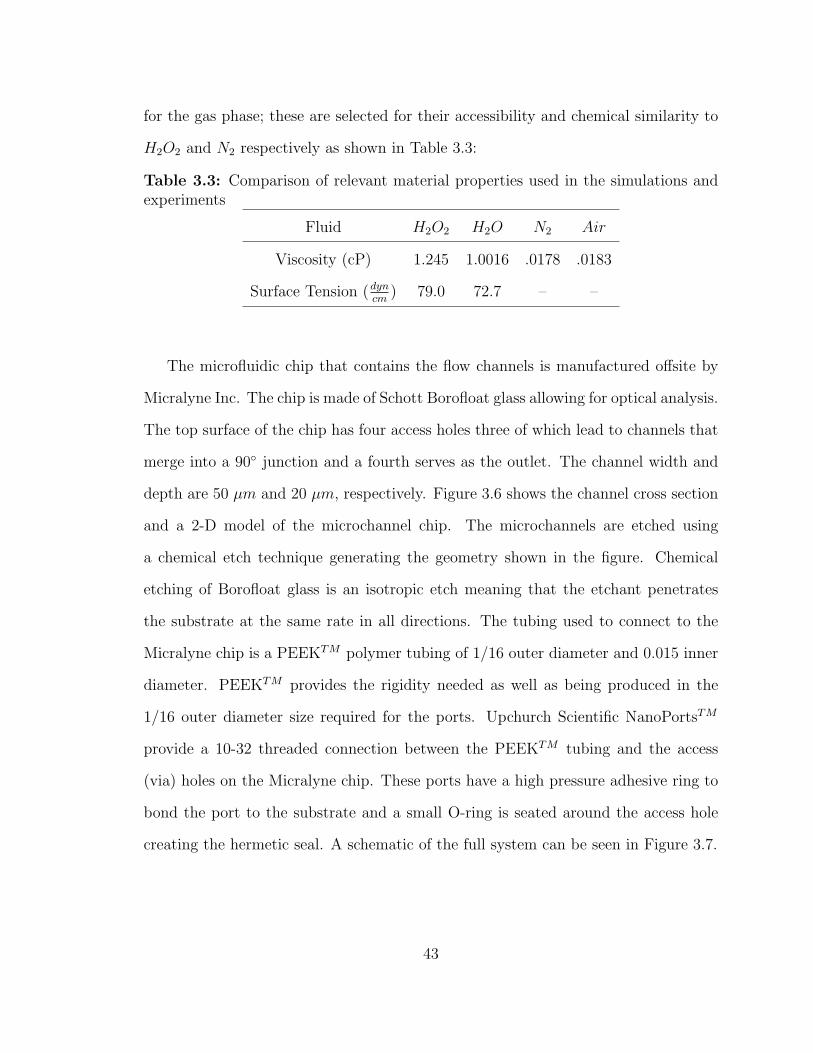
The microfluidic chip that contains the flow channels is manufactured offsite by
Micralyne Inc. The chip is made of Schott Borofloat glass allowing for optical analysis.
The top surface of the chip has four access holes three of which lead to channels that
merge into a 90◦ junction and a fourth serves as the outlet. The channel width and
depth are 50 µm and 20 µm, respectively. Figure 3.6 shows the channel cross section
and a 2-D model of the microchannel chip. The microchannels are etched using
a chemical etch technique generating the geometry shown in the figure. Chemical
etching of Borofloat glass is an isotropic etch meaning that the etchant penetrates
the substrate at the same rate in all directions. The tubing used to connect to the
Micralyne chip is a PEEKTM polymer tubing of 1/16 outer diameter and 0.015 inner
diameter. PEEKTM provides the rigidity needed as well as being produced in the
1/16 outer diameter size required for the ports. Upchurch Scientific NanoPortsTM
provide a 10-32 threaded connection between the PEEKTM tubing and the access
(via) holes on the Micralyne chip. These ports have a high pressure adhesive ring to
bond the port to the substrate and a small O-ring is seated around the access hole
creating the hermetic seal. A schematic of the full system can be seen in Figure 3.7.
43
Figure 3.6: a) Schematic of the microchannel chip layout. The insert shows thefour-way junction. b) Schematic of the microchannel cross section. The width ofthe mask line is 10 µm. The top piece of glass has the access holes and the bottompiece has the etched pattern. The two are fused together in the final steps of themanufacturing process.
3.4 Data Analysis
The goal of this study is to characterize the thruster characteristics, thrust and im-
pulse bit, as a function of varying parameters. To that end, it is necessary to isolate
the flow characteristics that are expected to vary during a simulation. To find the
thrust generated, assuming 100% efficiency in H2O2 decomposition, no viscous losses
in the micronozzle and no transient effects, was calculated using:
Ft = (ρLsAcf)Ispg0 (3.16)
where Ls is the average slug length, Ac is the cross-sectional area of the channel, f
is the slug formation frequency, Isp is the specific impulse of the monopropellant and
g0 is the acceleration due to gravity. The Isp of H2O2 is listed as 154s. In Equation
3.16, Ls and f are the only values that we expect to vary. For completeness, the
thrust contribution of the inert gas was also considered. Cold gas thrusters typically
have Isp values on the order of 70s or roughly half that of the H2O2. However, the
mass flow rate of the gas in this system is several magnitudes smaller than the liquid
44
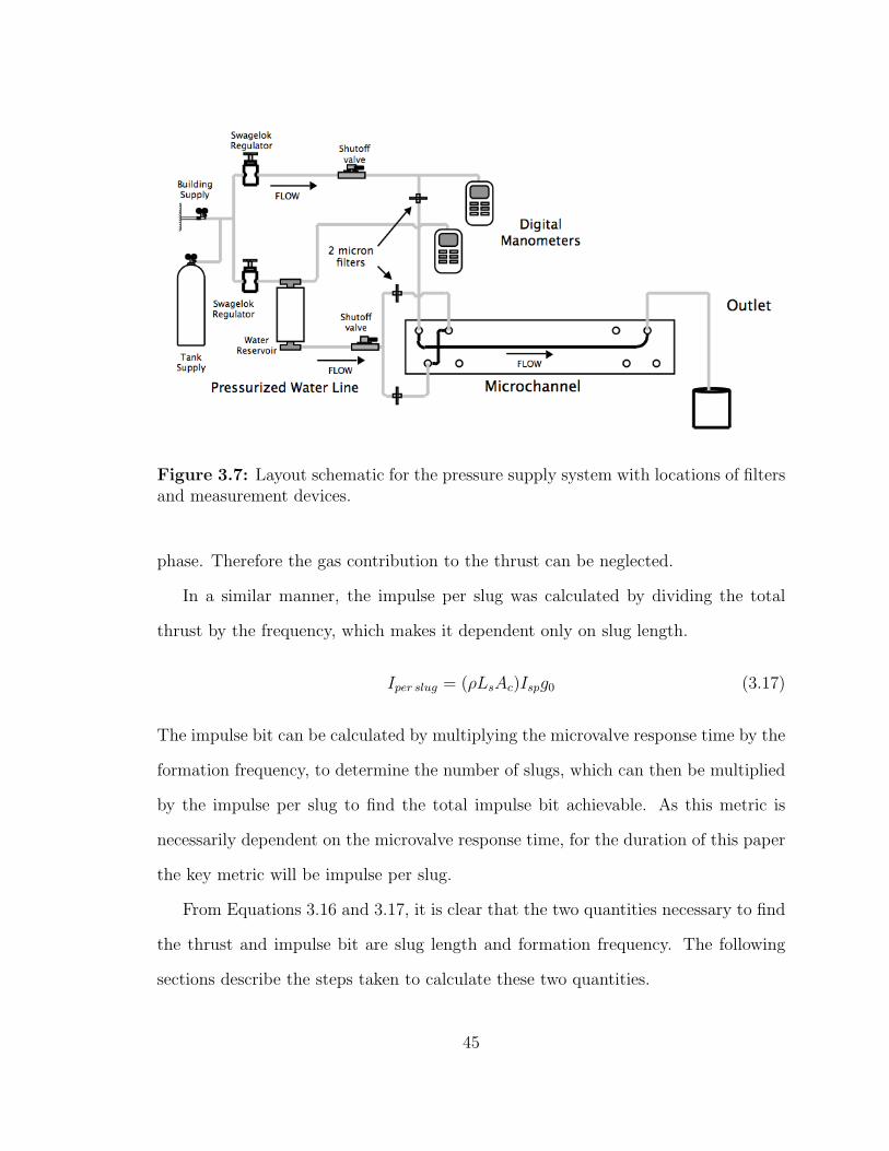
Figure 3.7: Layout schematic for the pressure supply system with locations of filtersand measurement devices.
phase. Therefore the gas contribution to the thrust can be neglected.
In a similar manner, the impulse per slug was calculated by dividing the total
thrust by the frequency, which makes it dependent only on slug length.
Iper slug = (ρLsAc)Ispg0 (3.17)
The impulse bit can be calculated by multiplying the microvalve response time by the
formation frequency, to determine the number of slugs, which can then be multiplied
by the impulse per slug to find the total impulse bit achievable. As this metric is
necessarily dependent on the microvalve response time, for the duration of this paper
the key metric will be impulse per slug.
From Equations 3.16 and 3.17, it is clear that the two quantities necessary to find
the thrust and impulse bit are slug length and formation frequency. The following
sections describe the steps taken to calculate these two quantities.
45
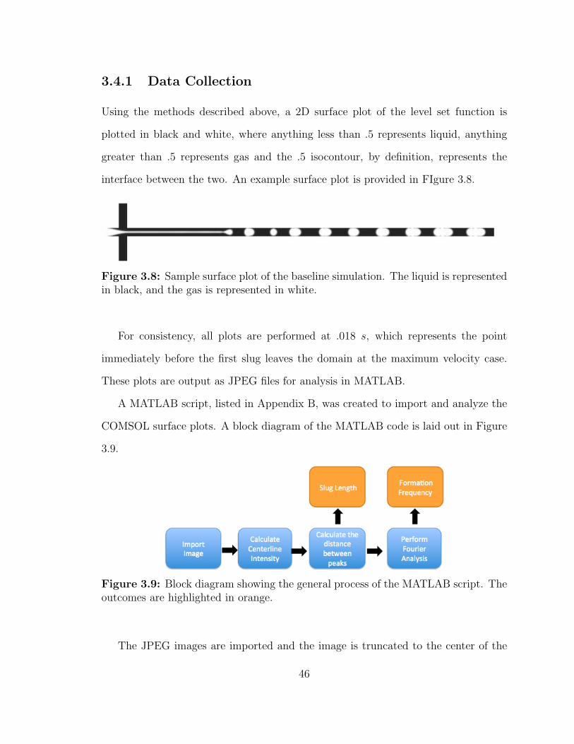
3.4.1 Data Collection
Using the methods described above, a 2D surface plot of the level set function is
plotted in black and white, where anything less than .5 represents liquid, anything
greater than .5 represents gas and the .5 isocontour, by definition, represents the
interface between the two. An example surface plot is provided in FIgure 3.8.
Figure 3.8: Sample surface plot of the baseline simulation. The liquid is representedin black, and the gas is represented in white.
For consistency, all plots are performed at .018 s, which represents the point
immediately before the first slug leaves the domain at the maximum velocity case.
These plots are output as JPEG files for analysis in MATLAB.
A MATLAB script, listed in Appendix B, was created to import and analyze the
COMSOL surface plots. A block diagram of the MATLAB code is laid out in Figure
3.9.
Figure 3.9: Block diagram showing the general process of the MATLAB script. Theoutcomes are highlighted in orange.
The JPEG images are imported and the image is truncated to the center of the
46
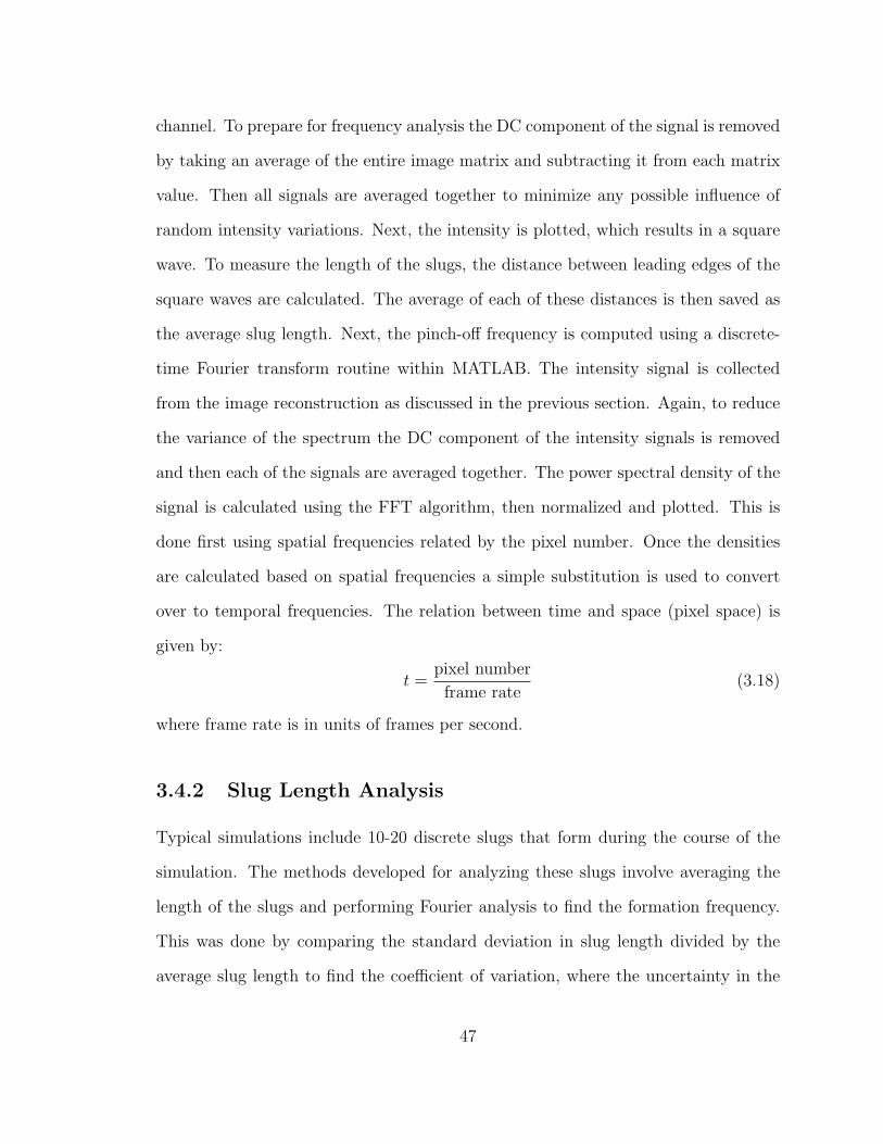
channel. To prepare for frequency analysis the DC component of the signal is removed
by taking an average of the entire image matrix and subtracting it from each matrix
value. Then all signals are averaged together to minimize any possible influence of
random intensity variations. Next, the intensity is plotted, which results in a square
wave. To measure the length of the slugs, the distance between leading edges of the
square waves are calculated. The average of each of these distances is then saved as
the average slug length. Next, the pinch-off frequency is computed using a discrete-
time Fourier transform routine within MATLAB. The intensity signal is collected
from the image reconstruction as discussed in the previous section. Again, to reduce
the variance of the spectrum the DC component of the intensity signals is removed
and then each of the signals are averaged together. The power spectral density of the
signal is calculated using the FFT algorithm, then normalized and plotted. This is
done first using spatial frequencies related by the pixel number. Once the densities
are calculated based on spatial frequencies a simple substitution is used to convert
over to temporal frequencies. The relation between time and space (pixel space) is
given by:
t =pixel number
frame rate(3.18)
where frame rate is in units of frames per second.
3.4.2 Slug Length Analysis
Typical simulations include 10-20 discrete slugs that form during the course of the
simulation. The methods developed for analyzing these slugs involve averaging the
length of the slugs and performing Fourier analysis to find the formation frequency.
This was done by comparing the standard deviation in slug length divided by the
average slug length to find the coefficient of variation, where the uncertainty in the
47
length of the microslugs comes from the lack of resolution in the images:
Coefficient of Variation =Standard Deviation
Average Slug Length(3.19)
In these studies, two types of periodic flows occurred: regular, periodic flow char-
acterized by slugs that had a coefficient of variation less than 5% and a flow regime
where consecutively numbered slugs would be periodic such that “odd” numbered
slugs are similar, and “even” numbered are similar, both with a coefficient of varia-
tion less than 5%. In typical thruster operation, hundreds of slugs may be produced
for a single maneuver, so these variations will become irrelevant.
Based on the similarity of slugs in both configurations, using average slug length
for the statistical calculations was deemed appropriate. All lengths reported in this
paper are averages of the finite number of slugs produced in the simulations.
3.4.3 Slug Volume Analysis
In Chapter 2, the mass flow rate of the microslugs was presented as:
m = (f ∗ Ls ∗ Ac ∗ ρ)
where f is the formation frequency, Ls is the length of a microslug, Ac is the cross-
sectional area of the microchannel and rho is the density of the fuel. This formulation,
first presented in McCabe [24], allows for the calculation of a mass flow rate using only
an average slug length. This formulation was ideal for the experimental procedures, as
it required a single measurement per slug, which could be taken along the centerline
of the channel, where the image was least distorted. There are some errors involved
in this calculation, as this method underestimates the volume of a microslug by
estimating it as a perfectly rectangular quadrahedron. McCabe [24] reported the
48
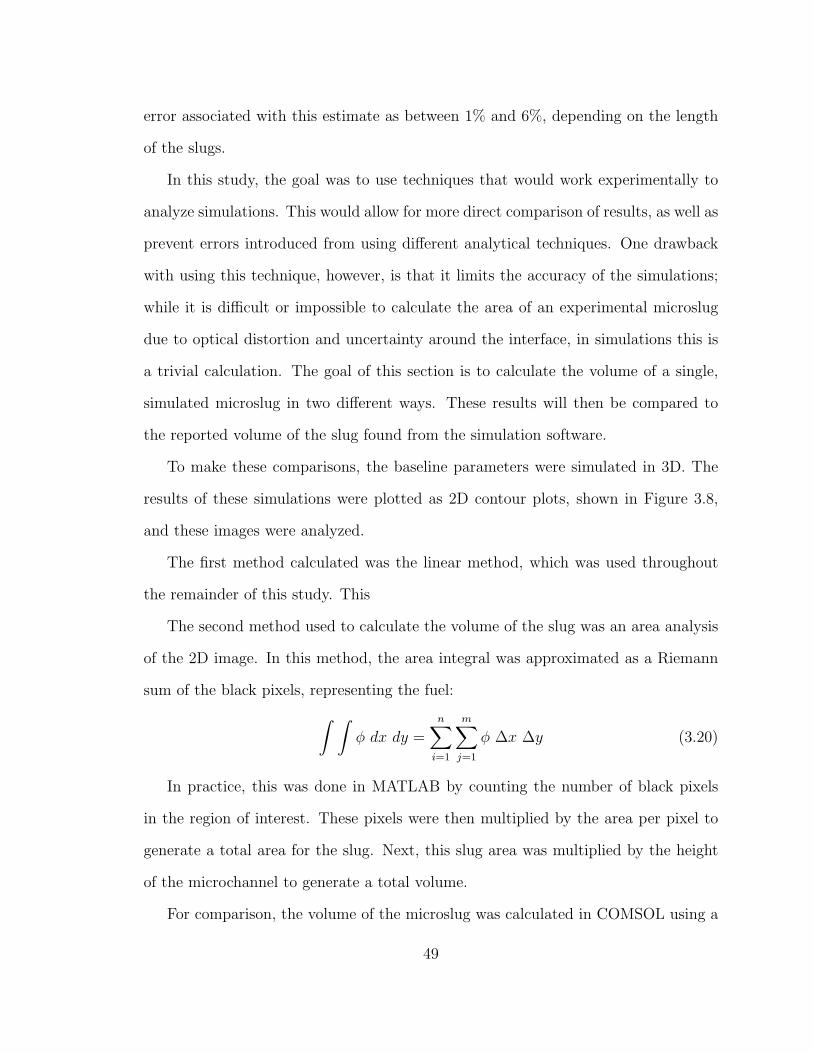
error associated with this estimate as between 1% and 6%, depending on the length
of the slugs.
In this study, the goal was to use techniques that would work experimentally to
analyze simulations. This would allow for more direct comparison of results, as well as
prevent errors introduced from using different analytical techniques. One drawback
with using this technique, however, is that it limits the accuracy of the simulations;
while it is difficult or impossible to calculate the area of an experimental microslug
due to optical distortion and uncertainty around the interface, in simulations this is
a trivial calculation. The goal of this section is to calculate the volume of a single,
simulated microslug in two different ways. These results will then be compared to
the reported volume of the slug found from the simulation software.
To make these comparisons, the baseline parameters were simulated in 3D. The
results of these simulations were plotted as 2D contour plots, shown in Figure 3.8,
and these images were analyzed.
The first method calculated was the linear method, which was used throughout
the remainder of this study. This
The second method used to calculate the volume of the slug was an area analysis
of the 2D image. In this method, the area integral was approximated as a Riemann
sum of the black pixels, representing the fuel:∫ ∫φ dx dy =
n∑i=1
m∑j=1
φ ∆x ∆y (3.20)
In practice, this was done in MATLAB by counting the number of black pixels
in the region of interest. These pixels were then multiplied by the area per pixel to
generate a total area for the slug. Next, this slug area was multiplied by the height
of the microchannel to generate a total volume.
For comparison, the volume of the microslug was calculated in COMSOL using a
49
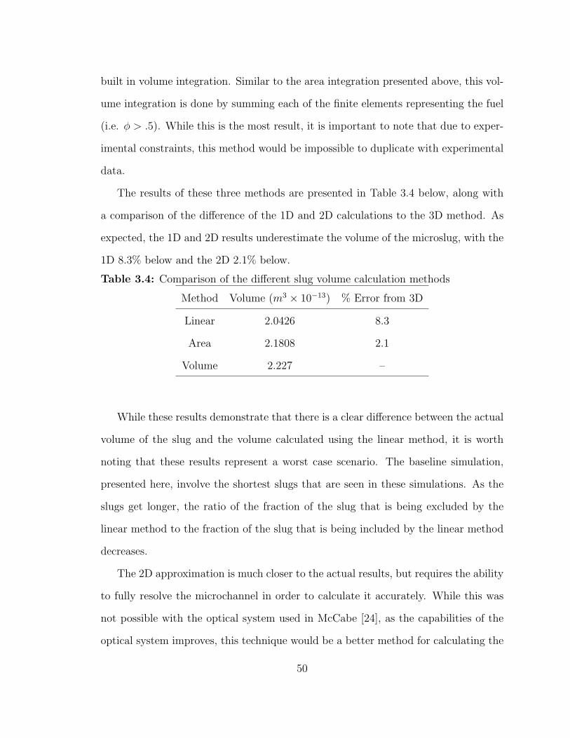
built in volume integration. Similar to the area integration presented above, this vol-
ume integration is done by summing each of the finite elements representing the fuel
(i.e. φ > .5). While this is the most result, it is important to note that due to exper-
imental constraints, this method would be impossible to duplicate with experimental
data.
The results of these three methods are presented in Table 3.4 below, along with
a comparison of the difference of the 1D and 2D calculations to the 3D method. As
expected, the 1D and 2D results underestimate the volume of the microslug, with the
1D 8.3% below and the 2D 2.1% below.
Table 3.4: Comparison of the different slug volume calculation methods
Method Volume (m3 × 10−13) % Error from 3D
Linear 2.0426 8.3
Area 2.1808 2.1
Volume 2.227 –
While these results demonstrate that there is a clear difference between the actual
volume of the slug and the volume calculated using the linear method, it is worth
noting that these results represent a worst case scenario. The baseline simulation,
presented here, involve the shortest slugs that are seen in these simulations. As the
slugs get longer, the ratio of the fraction of the slug that is being excluded by the
linear method to the fraction of the slug that is being included by the linear method
decreases.
The 2D approximation is much closer to the actual results, but requires the ability
to fully resolve the microchannel in order to calculate it accurately. While this was
not possible with the optical system used in McCabe [24], as the capabilities of the
optical system improves, this technique would be a better method for calculating the
50

volume of experimental slugs.
3.4.4 List of Studies
Using these methods parametric studies were performed, with surface tension coef-
ficient, contact angle and viscosity as the parameters of interest. For each of the
parameters two separate studies were conducted; the first held the inlet velocity for
both phases constant at .4 m/s while varying the parameter of interest. The second
held the parameter of interest constant while lowering the gas inlet in steps of .05
m/s. The full list of cases can be seen in the tables below.
51
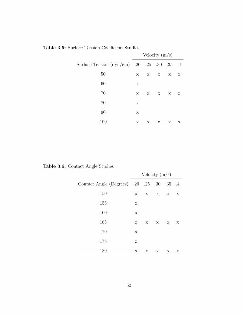
Table 3.5: Surface Tension Coefficient Studies
Velocity (m/s)
Surface Tension (dyn/cm) .20 .25 .30 .35 .4
50 x x x x x
60 x
70 x x x x x
80 x
90 x
100 x x x x x
Table 3.6: Contact Angle Studies
Velocity (m/s)
Contact Angle (Degrees) .20 .25 .30 .35 .4
150 x x x x x
155 x
160 x
165 x x x x x
170 x
175 x
180 x x x x x
52
Table 3.7: Fuel Viscosity Studies
Velocity (m/s)
Fuel Viscosity (cP) .20 .25 .30 .35 .4
0.6 x
0.8 x
1.0 x
1.2 x x x x x
1.4 x
1.6 x x x x x
1.8 x
53
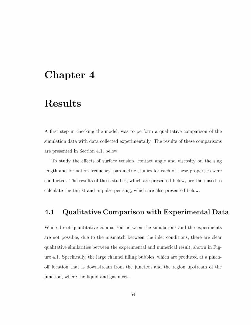
Chapter 4
Results
A first step in checking the model, was to perform a qualitative comparison of the
simulation data with data collected experimentally. The results of these comparisons
are presented in Section 4.1, below.
To study the effects of surface tension, contact angle and viscosity on the slug
length and formation frequency, parametric studies for each of these properties were
conducted. The results of these studies, which are presented below, are then used to
calculate the thrust and impulse per slug, which are also presented below.
4.1 Qualitative Comparison with Experimental Data
While direct quantitative comparison between the simulations and the experiments
are not possible, due to the mismatch between the inlet conditions, there are clear
qualitative similarities between the experimental and numerical result, shown in Fig-
ure 4.1. Specifically, the large channel filling bubbles, which are produced at a pinch-
off location that is downstream from the junction and the region upstream of the
junction, where the liquid and gas meet.
54
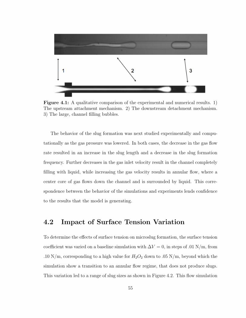
Figure 4.1: A qualitative comparison of the experimental and numerical results. 1)The upstream attachment mechanism. 2) The downstream detachment mechanism.3) The large, channel filling bubbles.
The behavior of the slug formation was next studied experimentally and compu-
tationally as the gas pressure was lowered. In both cases, the decrease in the gas flow
rate resulted in an increase in the slug length and a decrease in the slug formation
frequency. Further decreases in the gas inlet velocity result in the channel completely
filling with liquid, while increasing the gas velocity results in annular flow, where a
center core of gas flows down the channel and is surrounded by liquid. This corre-
spondence between the behavior of the simulations and experiments lends confidence
to the results that the model is generating.
4.2 Impact of Surface Tension Variation
To determine the effects of surface tension on microslug formation, the surface tension
coefficient was varied on a baseline simulation with ∆V = 0, in steps of .01 N/m, from
.10 N/m, corresponding to a high value for H2O2 down to .05 N/m, beyond which the
simulation show a transition to an annular flow regime, that does not produce slugs.
This variation led to a range of slug sizes as shown in Figure 4.2. This flow simulation
55
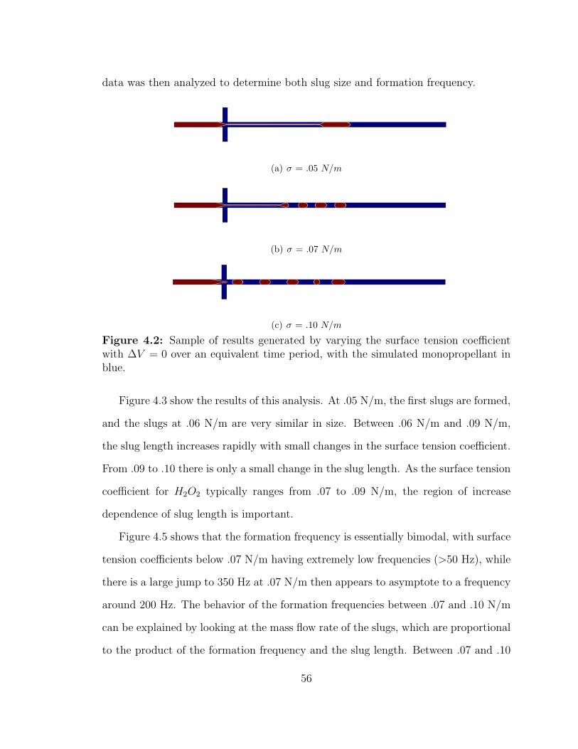
data was then analyzed to determine both slug size and formation frequency.
(a) σ = .05 N/m
(b) σ = .07 N/m
(c) σ = .10 N/m
Figure 4.2: Sample of results generated by varying the surface tension coefficientwith ∆V = 0 over an equivalent time period, with the simulated monopropellant inblue.
Figure 4.3 show the results of this analysis. At .05 N/m, the first slugs are formed,
and the slugs at .06 N/m are very similar in size. Between .06 N/m and .09 N/m,
the slug length increases rapidly with small changes in the surface tension coefficient.
From .09 to .10 there is only a small change in the slug length. As the surface tension
coefficient for H2O2 typically ranges from .07 to .09 N/m, the region of increase
dependence of slug length is important.
Figure 4.5 shows that the formation frequency is essentially bimodal, with surface
tension coefficients below .07 N/m having extremely low frequencies (>50 Hz), while
there is a large jump to 350 Hz at .07 N/m then appears to asymptote to a frequency
around 200 Hz. The behavior of the formation frequencies between .07 and .10 N/m
can be explained by looking at the mass flow rate of the slugs, which are proportional
to the product of the formation frequency and the slug length. Between .07 and .10
56
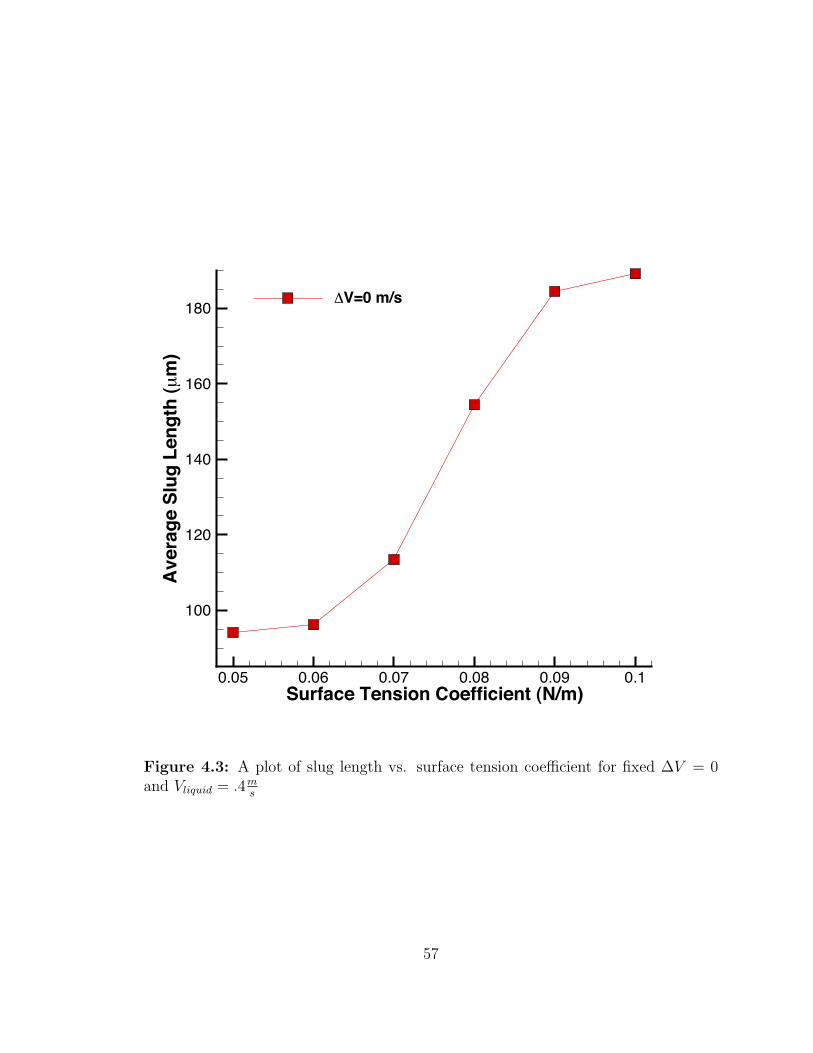
Surface Tension Coefficient (N/m)
Ave
rage
Slu
g Le
ngth
(!m
)
0.05 0.06 0.07 0.08 0.09 0.1
100
120
140
160
180�V=0 m/s
Figure 4.3: A plot of slug length vs. surface tension coefficient for fixed ∆V = 0and Vliquid = .4m
s
57
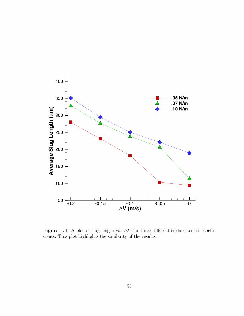
�V (m/s)
Ave
rage
Slu
g Le
ngth
(µm
)
-0.2 -0.15 -0.1 -0.05 050
100
150
200
250
300
350
400
.05 N/m
.07 N/m
.10 N/m
Figure 4.4: A plot of slug length vs. ∆V for three different surface tension coeffi-cients. This plot highlights the similarity of the results.
58
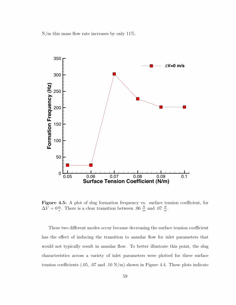
N/m this mass flow rate increases by only 11%.
Surface Tension Coefficient (N/m)
Form
atio
n Fr
eque
ncy
(Hz)
0.05 0.06 0.07 0.08 0.09 0.10
50
100
150
200
250
300
350�V=0 m/s
Figure 4.5: A plot of slug formation frequency vs. surface tension coefficient, for∆V = 0m
s. There is a clear transition between .06 N
mand .07 N
m.
These two different modes occur because decreasing the surface tension coefficient
has the effect of inducing the transition to annular flow for inlet parameters that
would not typically result in annular flow. To better illustrate this point, the slug
characteristics across a variety of inlet parameters were plotted for three surface
tension coefficients (.05, .07 and .10 N/m) shown in Figure 4.4. These plots indicate
59
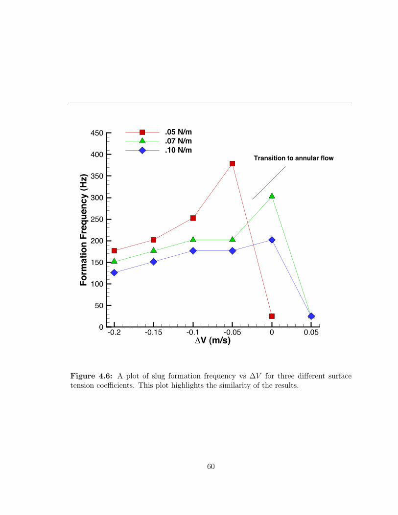
�V (m/s)
Form
atio
n Fr
eque
ncy
(Hz)
-0.2 -0.15 -0.1 -0.05 0 0.050
50
100
150
200
250
300
350
400
450 .05 N/m.07 N/m.10 N/m
Transition to annular flow
Figure 4.6: A plot of slug formation frequency vs ∆V for three different surfacetension coefficients. This plot highlights the similarity of the results.
60
that the effect of surface tension acts as an offset for the slug formation, where an
increase in the surface tension coefficient has an effect similar to increasing the gas
inlet velocity. Figure 4.6 shows the low surface tension coefficient case transitioning
from slugs to annular flow for a lower gas inlet velocity.
4.3 Impact of Contact Angle Variation
The next parameter of interest was the sensitivity of slug formation to changes in the
contact angle. Contact angle, which is a measure of the hydrophobicity of the surface
of the microchannel, can be modified by contaminants in the liquid or imperfections
in walls and could have an impact on the performance of the system. Shown in Figure
4.7 are plots of the slug size and formation frequency as a function of contact angle
for a fixed inlet condition (∆V = 0) and surface tension coefficient (.07 N/m). This
plot indicates a bimodal structure with a transition between 150 and 160 degrees.
The physical mechanism for this transition is readily observed in Figure 4.8, where
the pinch-off location shifts from the junction (≤155 Degrees) to a pinch-off located
several channel widths downstream (>155 degrees).
This shift in pinch-off location appears to be connected with the attachment point
that exists upstream of the junction; as the contact angle varies the angle that this
attachment point makes with the wall varies accordingly. For values of the contact
angle equal to or below 155 degrees, the angle of this attachment results in slugs
generated at the junction. As the contact angle increases, a critical value is reached
at which the attachment point no longer results in slugs being formed at the junction,
shifting to a downstream pinch-off. While dramatic shifts in the contact angle are
unexpected during typical operation, this connection between the detachment point,
and the corresponding slug length, indicates that the microchannel should be designed
61
Contact Angle (Degrees)
Ave
rage
Slu
g Le
ngth
(!m
)
140 150 160 170 180105
110
115
120
125
130
135
140
145
150
155
�V = 0 m/s
Transition from pinch-off at junctionto downstream pinch-off
Tranto do
Figure 4.7: The plot of slug length as a function of contact angle. There is a cleartransition between 155 and 160 degrees, which corresponds to a change in pinch-offmechanism.
62
to avoid this transition region.
(a) Contact Angle = 155◦
(b) Contact Angle = 160◦
Figure 4.8: Contour plots showing the change in detachment location that leads tochange in microslug length.
Next, the system was simulated for three different contact angles as the air inlet
velocity was increased. Figure 4.9 is a plot of the average slug length for 150, 165
and 180 degrees. This plot shows that increasing contact angle has an inconsistent
effect on the slug length.
4.4 Impact of Thermally-Induced
Viscosity Variation
The final parameter studied was the sensitivity of the system to minor changes in
viscosity. In Cubaud et al.[31], variations in the viscosity ratio of the two fluids were
shown to have a significant effect on the flow regime. Specifically, as the viscosity
ratio of the liquid phase to the gas phase increases, there can be a transition from
a slug forming regime to annular flow. As the viscosity of H2O2 ranges from .6 cP
at 50◦ C to 1.8 cP at 0◦ C, the microthruster may undergo significant changes in
63
6V (m/s)
Ave
rage
Slu
g Le
ngth
(µm
)
0.2 0.25 0.3 0.35 0.430
40
50
60
70
80
90
100
110
120
130
140
150
150 Degrees165 Degrees180 Degrees
Figure 4.9: A plot of slug length vs. ∆V for three different contact angles. Thisplot highlight the similarity of the results for these contact angles.
64
the viscosity ratio during operation. To determine the effects of these changes, the
viscosity of the liquid phase was varied from .6 cP to 1.8 cP in steps of .2 cP.
Plots of the slug length and formation frequency for various viscosities are shown
in Figures 4.10 and 4.11. From .6 to 1.6 cP there is a 47.16% reduction in slug length,
but there is a smooth, nearly linear progression. At 1.8 cP, however, the system
transitions from slug formation to annular flow in a manner that appears consistent
with the work presented in Cubaud et al. As no slugs are formed, the slug length and
formation frequency drop to zero in this case.
To understand the plot of formation frequency, it is again illustrative to look at
the mass flow rate by taking the product of the slug length and formation frequency.
When this is done, there are two distinct regions where the mass flow rate is relatively
unchanged. In the first region, between .6 and 1.0 cP, the mass flow rate decreases by
6%. Between 1.0 cP and 1.2 cP, the mass flow rate decreases by 39%. Then, between
1.2 and 1.6 cP, the mass flow rate decreases by 19%.
Further studies were done to determine the relationship between slug formation
and air inlet velocity as the viscosity of the fuel is increased. As shown in Figure 4.12,
there is a strong similarity between the length of the slugs at 1.2 cP and1.6 cP, with
the increased viscosity acting to decrease the length of the slugs.
In Figure 4.13, the slug formation frequency is plotted for increasing air inlet
velocity. The higher viscosity results in an increase in the slug formation frequency.
The plot shows a clear similarity between the formation frequency of the system at
the two different viscosities.
65
Viscosity (cP)
Ave
rage
Slu
g Le
ngth
(!m
)
0.6 0.7 0.8 0.9 1 1.1 1.2 1.3 1.4 1.5 1.6 1.7 1.8-20
0
20
40
60
80
100
120
140
160
180
200
�V=0 m/s
Figure 4.10: A plot of slug length vs. fuel viscosity for ∆V = 0. At 1.8 cP, thesystem transitions to annular flow, with no slugs being made.
66
Viscosity (cP)
Form
atio
n Fr
eque
ncy
(Hz)
0.6 0.8 1 1.2 1.4 1.6 1.8
0
50
100
150
200
250
300
�V=0 m/s
Figure 4.11: A plot of slug formation frequency vs. fuel viscosity for ∆V = 0. Asthe system transitions to annular flow at 18 cP, the formation frequency drops to 0.
4.5 Effective Impulse and Thrust
The effects of the changes in slug length and formation frequency on the thrust are
plotted below. For comparison, the baseline thrust of the system was calculated and
plotted as well. The maximum thrust of a monopropellant thruster can be calculated
67
6V (m/s)
Visc
osity
(cP)
0.2 0.25 0.3 0.35 0.40
20
40
60
80
100
120
140
160
1.2 cP1.6 cP
Figure 4.12: A plot of slug length vs. ∆V for two different fuel viscosities. Thereis a clear similarity between the two solutions.
68
6V (m/s)
Form
atio
n Fr
eque
ncy
(Hz)
0.2 0.25 0.3 0.35 0.4100
150
200
250
300
3501.2 cP1.6 cP
Figure 4.13: A plot of slug formation frequency vs. ∆V for two different fuelviscosities. There is a clear similarity between the two solutions.
69
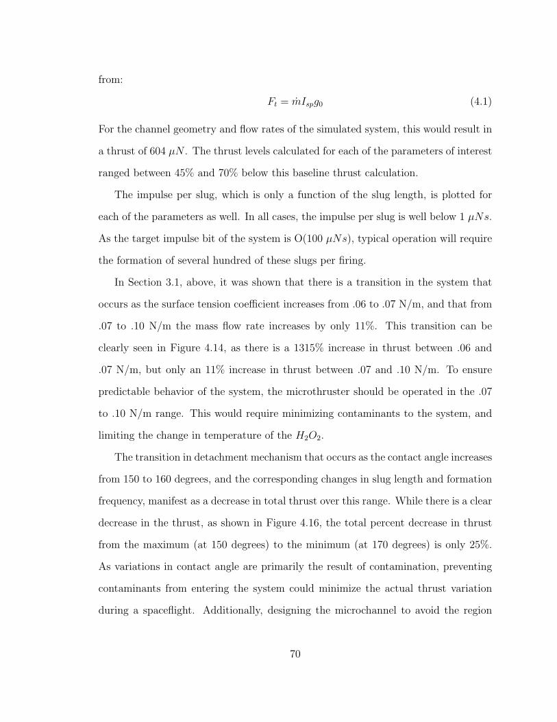
from:
Ft = mIspg0 (4.1)
For the channel geometry and flow rates of the simulated system, this would result in
a thrust of 604 µN . The thrust levels calculated for each of the parameters of interest
ranged between 45% and 70% below this baseline thrust calculation.
The impulse per slug, which is only a function of the slug length, is plotted for
each of the parameters as well. In all cases, the impulse per slug is well below 1 µNs.
As the target impulse bit of the system is O(100 µNs), typical operation will require
the formation of several hundred of these slugs per firing.
In Section 3.1, above, it was shown that there is a transition in the system that
occurs as the surface tension coefficient increases from .06 to .07 N/m, and that from
.07 to .10 N/m the mass flow rate increases by only 11%. This transition can be
clearly seen in Figure 4.14, as there is a 1315% increase in thrust between .06 and
.07 N/m, but only an 11% increase in thrust between .07 and .10 N/m. To ensure
predictable behavior of the system, the microthruster should be operated in the .07
to .10 N/m range. This would require minimizing contaminants to the system, and
limiting the change in temperature of the H2O2.
The transition in detachment mechanism that occurs as the contact angle increases
from 150 to 160 degrees, and the corresponding changes in slug length and formation
frequency, manifest as a decrease in total thrust over this range. While there is a clear
decrease in the thrust, as shown in Figure 4.16, the total percent decrease in thrust
from the maximum (at 150 degrees) to the minimum (at 170 degrees) is only 25%.
As variations in contact angle are primarily the result of contamination, preventing
contaminants from entering the system could minimize the actual thrust variation
during a spaceflight. Additionally, designing the microchannel to avoid the region
70
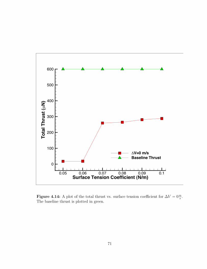
Surface Tension Coefficient (N/m)
Tota
l Thr
ust (!
N)
0.05 0.06 0.07 0.08 0.09 0.1
0
100
200
300
400
500
600
�V=0 m/sBaseline Thrust
Figure 4.14: A plot of the total thrust vs. surface tension coefficient for ∆V = 0ms
.The baseline thrust is plotted in green.
71
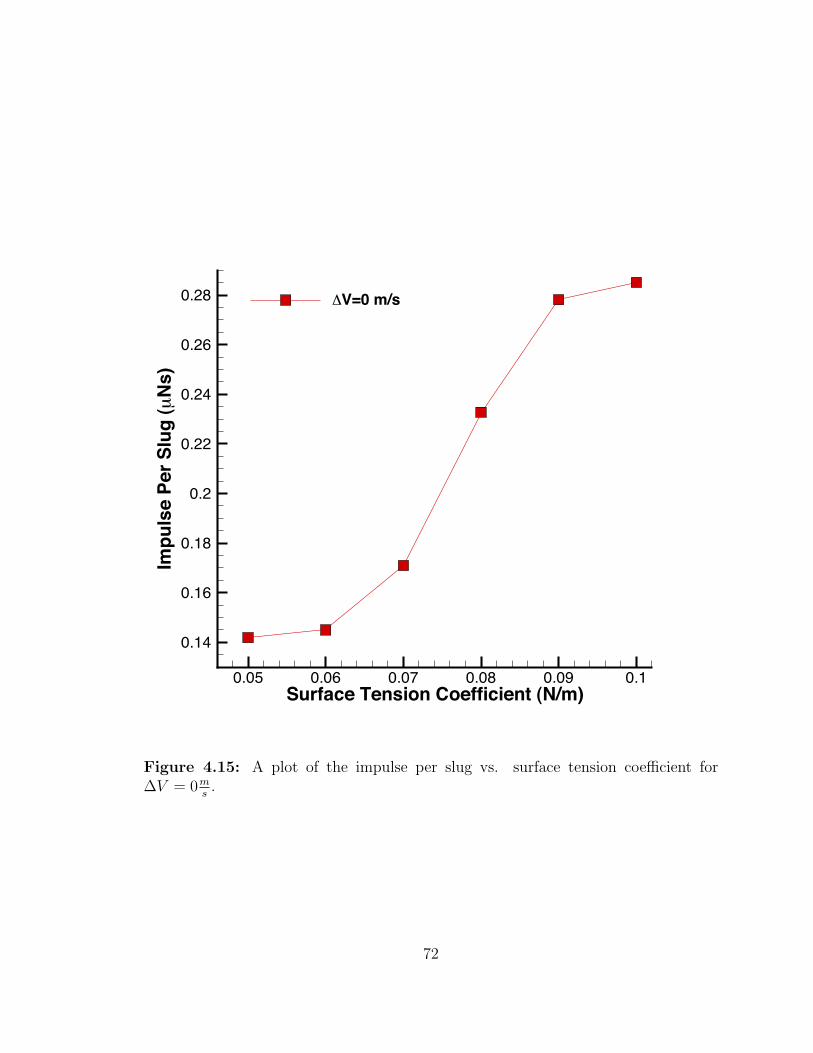
Surface Tension Coefficient (N/m)
Impu
lse
Per S
lug
(!N
s)
0.05 0.06 0.07 0.08 0.09 0.1
0.14
0.16
0.18
0.2
0.22
0.24
0.26
0.28 �V=0 m/s
Figure 4.15: A plot of the impulse per slug vs. surface tension coefficient for∆V = 0m
s.
72
between 150 and 160 degrees would result in more stable operation.
Contact Angle (Degrees)
Tota
l Thr
ust (!
N)
140 150 160 170 180
250
300
350
400
450
500
550
600
�V=0 m/sBaseline Thrust
Figure 4.16: A plot of total thrust vs. contact angle for ∆V = 0ms
. The baselinethrust is plotted in green.
The thrust as a function of changes in viscosity, shown in Figure 4.18, shows that
there are two different thrust regions that exist in the system. In the first, between
.6 and 1.0 cP, the thrust starts at 277 µN and decreases by 6%. From 1.0 to 1.2 cP,
the thrust decreases by 38% to 159 µN , then from 1.2 to 1.6 cP the thrust decreases
by 19%. At 1.8 cP no slugs are produced, and thus the thrust goes to zero. This
73
Contact Angle (Degrees)
Impu
lse
Per S
lug
(!N
s)
140 150 160 170 180
0.16
0.18
0.2
0.22
0.24
�V=0 m/s
Figure 4.17: A plot of impulse per slug vs. contact angle for ∆V = 0ms
.
74
seems to show that there are two stable regions of operation, with the region between
.6 and 1.0 cP, which corresponds to the temperature range of 50◦ to 25◦, being the
most stable. Designing the system to maintain the temperature of the H2O2 in this
range, should allow for stable operation of the system.
Viscosity (cP)
Tota
l Thr
ust (!
N)
0.6 0.8 1 1.2 1.4 1.6 1.8
0
100
200
300
400
500
600
�V=0 m/sBaseline Thrust
Figure 4.18: A plot of total thrust vs. viscosity for ∆V = 0ms
. The baseline thrustis plotted in green.
75
Viscosity (cP)
Impu
lse
Per S
lug
(!N
s)
0.6 0.8 1 1.2 1.4 1.6 1.8
0
0.05
0.1
0.15
0.2
0.25
0.3
�V=0 m/s
Figure 4.19: A plot of impulse per slug vs. viscosity for ∆V = 0ms
.
76
Chapter 5
Conclusions
In this study, a computational model of dispersed slug formation at a microchannel
junction was developed and used to examine the sensitivity of the slug characteristics
to important material properties. The envisioned application of the slug formation
is that of a discrete H2O2 monopropellant fuel injection scheme for nanosat micro-
propulsion. Given the extremely low thrust and impulse levels involved, the sensitivity
analysis is quite important in assessing design robustness. Specifically, the effects of
variable surface tension, contact angle and fuel viscosity were examined; these varia-
tions might arise naturally under conditions of system contamination and/or thermal
variations.
For each of the parameters studied, there exist regions where the small changes
in the material property can cause the flow to transition from one slug formation
regime to another, with a corresponding discontinuous change in slug formation char-
acteristics. In the case of the surface tension coefficient, this transition starts at .06
N/m; above this value the slug length increases rapidly before stabilizing around .09
N/m. The contact angle influences the slug length by causing a shift in the location
of the slug formation; for values less than 150 degrees the slugs are formed at the
77
junction, while values greater than 160 degrees result in a downstream pinch-off with
smaller slugs. As the viscosity of the fuel is increased, the slug length decreases until
it transitions to annular flow for values larger than 1.6 cP.
The thrust and impulse per slug were calculated using the slug length and forma-
tion frequency, and so they show similar discontinuous profiles as the parameters are
varied. Outside of these transition regions, however, there are stable regions where
the thrust is smooth. For surface tension, this stable region exists between .07 N/m
and .10 N/m where thrust decreases by 11%. As the contact angle increases from 140
and 155 degrees, the thrust decreases by 5%. There is a region between 155 and 170
degrees where the thrust drops by 25%, and between 170 and 180 degrees, the thrust
increases by 14%. The thrust as a function of viscosity exhibits two stable regions,
one between .6 and 1.0 cP where there is a 6% decrease in thrust, and the second
between 1.2 to 1.6 cP where there is a 19% decrease in thrust.
The sensitivity of the slug characteristics, and hence thrust and impulse pro-
duction, under certain flow conditions presents an area for concern for the overall
robustness of the discrete monopropellant fuel injection scheme. Yet there are also
highly stable regions where the slug characteristics are essentially insensitive to prop-
erty variations. It follows, therefore, that future microthruster system designs should
target and incorporate these stable flow regions in their baseline operating conditions
to maximize operational robustness.
5.1 Future Work
There are several efforts that could be undertaken to further the studies discussed
in this thesis. As discussed in Chapter 3, a 2D model of the system was used to
ensure the greatest number of simulations could be performed. During the course
78
of this work, advances in computer processing power as well as improvements in the
COMSOL software have made studies of a 3D model a realistic goal. While the results
of the 2D simulations compare closely with the 3D model examined, it is possible that
in certain regimes, there are 3D effects that are not being captured in the current
simulations. With this in mind, a fully 3D simulation of the channels would be a
clear next step.
A second area of interest for future study would be using the simulations to op-
timize the geometry of the system. The original 90◦ junction was selected for its
availability in off-the-shelf microchannels due to the ease of manufacture. As MEMS
fabrication techniques have continued to improve, it is now possible to create the
microchannel junction over a much wider intersection angle. Additionally, the simu-
lations could be used to identify the miniaturization limit of the system.
79
References
[1] J. Mueller, Thruster options for microspacecraft: a review and evaluation of the
state-of-the art and emerging technologies, in Micropropulsion for Small Space-
craft - Progress in Astronautics and Aeronautics, M. Micci and A. Ketsdever,
eds., vol. 187, AIAA, Reston, Va., p. 45-137, 2000.
[2] S. Janson, The History of Small Satellites, In H. Helvajian and S. Janson (Eds.).
Small Satellites: Past, Present and Future. (pp. 45-87). El Segundo, CA, 2008.
[3] J. Mueller, C. Marrese, J. Polk, EH. Yang, A. Green, V. White, D. Bame, I.
Chakraborty, S. Vargo, R. Reinicke, An Overview of MEMS-based micropropul-
sion developments at JPL, ACTA ASTRONAUTICA, Vol. 52, Issue 9-12, p.
881-895, May-June 2003.
[4] S. Marcuccio, A. Genovese, M. Andrenucci, FEEP MICROTHRUSTER TECH-
NOLOGY STATUS AND POTENTIAL APPLICATIONS, 48th International
Astronautical Federation Congress, Turin, Italy, 1997.
[5] J. Baker, P. Bender, P. Binetruy, et al, LISA: Probing the Uni-
verse with Gravitational Waves, Version 1.0, LISA Mission Science Office,
http://lisa.jpl.nasa.gov/news.html, January 19, 2007.
80
[6] M. Neugebauer, C. W. Snyder, Solar Plasma Experiment, Science, Vol. 138, No.
3545, pp. 1095 - 1097, 7 December, 1962.
[7] R. J. Bzibziak, Sr., Miniature cold gas thrusters, AIAA-1992-3256, SAE, ASME,
and ASEE, Joint Propulsion Conference and Exhibit, 28th, Nashville, TN July
6-8, 1992.
[8] J. Mueller, W. Tang, A. Wallace, W. Li, D. Bame, I. Chakraborty and R. Lawton,
Design, Analysis, and Fabrication of a Vaporizing Liquid Micro-Thruster, AIAA
Paper 98-3924, 34th Joint Propulsion Conference, Cleveland, OH, July 1998.
[9] D. L. Hitt, C. M. Zakrzwski, M. K. Thomas, MEMS-Based Satellite Micropropul-
sion Via Catalyzed Hydrogen Peroxide Decomposition, Smart Mater. Struct., 10,
1163-1175, 2001.
[10] R. A. W. Fleron, J. H. Hales, A MEMS Based Field Emission Electrical Propul-
sion System With Integrated Charge Neutralizer For Nano And Pico Spacecraft,
Proceedings of the 4th International Spacecraft Propulsion Conference (ESA SP-
555), Cagliari, Italy, 2-9 June, 2004.
[11] C. Scharlemann, M. Tajmar, Development of Propulsion Means For Microsatel-
lites, AIAA-2007-5184, 43rd AIAA/ASME/SAE/ASEE Joint Propulsion Con-
ference and Exhibit, Cincinnati, OH, July 2007
[12] J. Nabity, G. Mason, J. Engel, J. Daily, R. Laumbay, D. Kassoy, Studies of
MEMS Colloid Thrusters, AIAA-2006-5007, 42nd AIAA/ASME/SAE/ASEE
Joint Prop. Conf. and Exhibit, Sacramento, CA, July 9-12, 2006.
81
[13] J. Xiong, Z. Zhou, D. Sun, X. Ye, Development of a MEMS based colloid thruster
with sandwich structure, Sensors & Actuators A, Vol. 117, Issue 1, pp. 168-172,
January 2005.
[14] D. Lewis, Jr., S. Janson, R. Cohen, Digital MicroPropulsion,, 12th IEEE Inter-
national Conference on Micro Electro Mechanical Systems, pp. 517-52, 1999.
[15] P. Fuqua, S.W. Janson, W. Hansen, H.Helvajian, Fabrication of true 3D mi-
crostructures in glass/ceramic materials by pulsed UV laser volumetric exposure
techniques, Proc. SPIE, p 213, 1999.
[16] R. Bayt, Analysis, Fabrication and Testing of a MEMS-based Micropropulsion
System, FDRL TR 99-1, Ph.D. Thesis supervised by Prof. Kenneth Breuer,
M.I.T. Dept. of Aeronautics and Astronautics, June, 1999.
[17] J. Blandino, M. McDevitt, J. Mueller, D. Bame, & A. Green. Characterization
of dryout point in the vaporizing liquid microthruster. Journal of Propulsion and
Power, 22(3), 677683, 2006.
[18] J. Mueller. Review and Applicability Assessment of MEMS-Based Microvalve
Technologies for Microspacecraft Propulsion, Micropropulsion for Small Space-
craft, Progress in Astronautics and Aeronautics, Vol. 187, edited by M. Micci
and A. Ketsdever, AIAA, Reston, VA, pp. 449-476, 2000.
[19] K. W. Oh, C. H. Ahn, A review of microvalves, J. of Micromech. and Microeng.,
16, R13-R39, 2006.
[20] J. McCabe & D. Hitt, Monopropellant fuel injection using two-phase micro-slug
formation. Proceedings of 39th Annual AIAA Fluid Dynamics Conference, 2009.
82
[21] T.R. Harris, D.L. Hitt, and R.G. Jenkins, Discrete Micro-Slug Formation for
Micro-Thruster Propellant Delivery, AIAA Paper 2005-0676, 2005.
[22] T. Cubaud and C. Ho, Transport of bubbles in square microchannels, Physics of
Fluids, Volume 16, No 12, pp. 4575-85, 2004.
[23] T. Cubaud, M. Tatineni, X. Zhong, and C. M. Ho, Bubble dispenser in microflu-
idic devices, Phys. Review E, 72, 037302, 2005.
[24] J.W. McCabe, Monopropellant Fuel Injection Using Two-Phase Micro-Slug For-
mation. (Master’s Thesis) University of Vermont, Burlington, VT, 2009.
[25] J. Sethian. Level set methods and fast marching methods: evolving interfaces in
computational geometry, fluid mechanics, computer vision, and materials science,
1999.
[26] A.K. Tornberg, B. Enhquist, A finite element based level set method for multi-
phase flow applications, Comput. Visual. Sci. 3, 93-101, 2000.
[27] E. Olsson & G. Kreiss, A conservative level set method for two phase flow.
Journal of Computational Physics, 2005.
[28] E. Olsson & G. Kreiss, A conservative level set method for two phase flow II.
Journal of Computational Physics, 2007.
[29] N.A. Mortensen, F. Okkels, H. Bruus, Reexamination of Hagen-Poiseuille flow:
Shape dependence of the hydraulic resistance in microchannels, Phys. Rev. E,
71, 057301, 2005.
[30] D. Qian & A. Lawal. Numerical study on gas and liquid slugs for Taylor flow in
a T-junction. Chemical Engineering Science, 2006.
83

[31] T. Cubaud & T. Mason, Capillary threads and viscous droplets in square mi-
crochannels. Physics of Fluids, 2008.
84
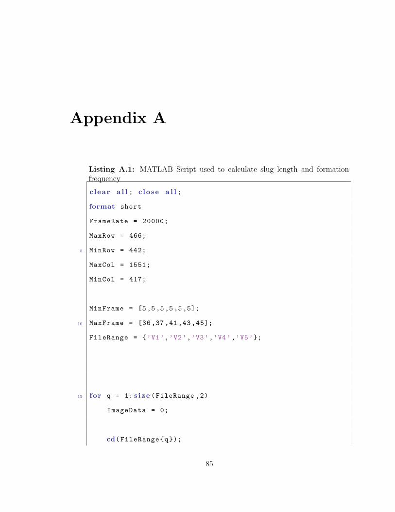
Appendix A
Listing A.1: MATLAB Script used to calculate slug length and formationfrequency
c lear a l l ; c lose a l l ;
format short
FrameRate = 20000;
MaxRow = 466;
5 MinRow = 442;
MaxCol = 1551;
MinCol = 417;
MinFrame = [5,5,5,5,5,5];
10 MaxFrame = [36 ,37 ,41 ,43 ,45];
FileRange = {’V1’,’V2’,’V3’,’V4’,’V5’};
15 for q = 1: s i ze (FileRange ,2)
ImageData = 0;
cd(FileRange{q});
85
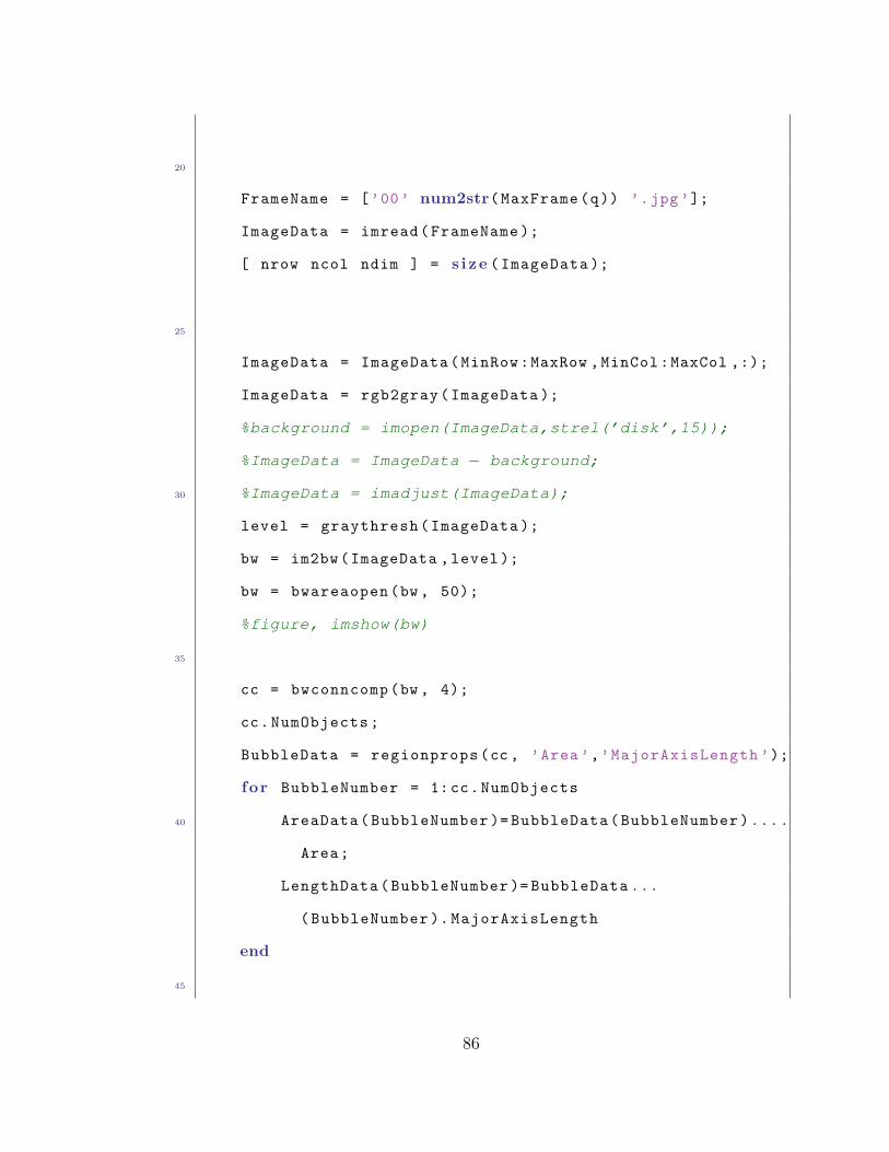
20
FrameName = [’00’ num2str(MaxFrame(q)) ’.jpg’];
ImageData = imread(FrameName );
[ nrow ncol ndim ] = s i ze (ImageData );
25
ImageData = ImageData(MinRow:MaxRow ,MinCol:MaxCol ,:);
ImageData = rgb2gray(ImageData );
%background = imopen(ImageData,strel(’disk’,15));
%ImageData = ImageData − background;
30 %ImageData = imadjust(ImageData);
level = graythresh(ImageData );
bw = im2bw(ImageData ,level );
bw = bwareaopen(bw, 50);
%figure, imshow(bw)
35
cc = bwconncomp(bw, 4);
cc.NumObjects;
BubbleData = regionprops(cc, ’Area’,’MajorAxisLength ’);
for BubbleNumber = 1:cc.NumObjects
40 AreaData(BubbleNumber )= BubbleData(BubbleNumber)....
Area;
LengthData(BubbleNumber )= BubbleData ...
(BubbleNumber ). MajorAxisLength
end
45
86
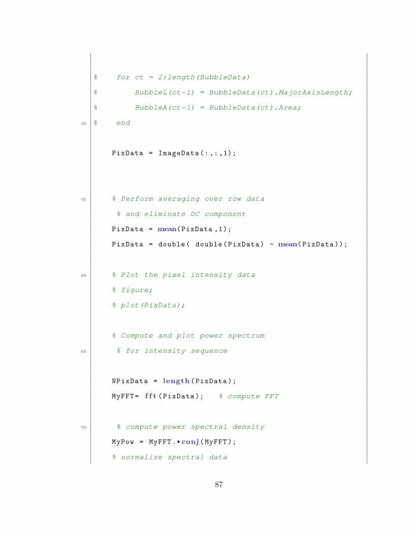
% for ct = 2:length(BubbleData)
% BubbleL(ct−1) = BubbleData(ct).MajorAxisLength;
% BubbleA(ct−1) = BubbleData(ct).Area;
50 % end
PixData = ImageData (:,:,1);
55 % Perform averaging over row data
% and eliminate DC component
PixData = mean(PixData ,1);
PixData = double( double(PixData) - mean(PixData ));
60 % Plot the pixel intensity data
% figure;
% plot(PixData);
% Compute and plot power spectrum
65 % for intensity sequence
NPixData = length(PixData );
MyFFT= f f t (PixData ); % compute FFT
70 % compute power spectral density
MyPow = MyFFT .* conj(MyFFT );
% normalize spectral data
87
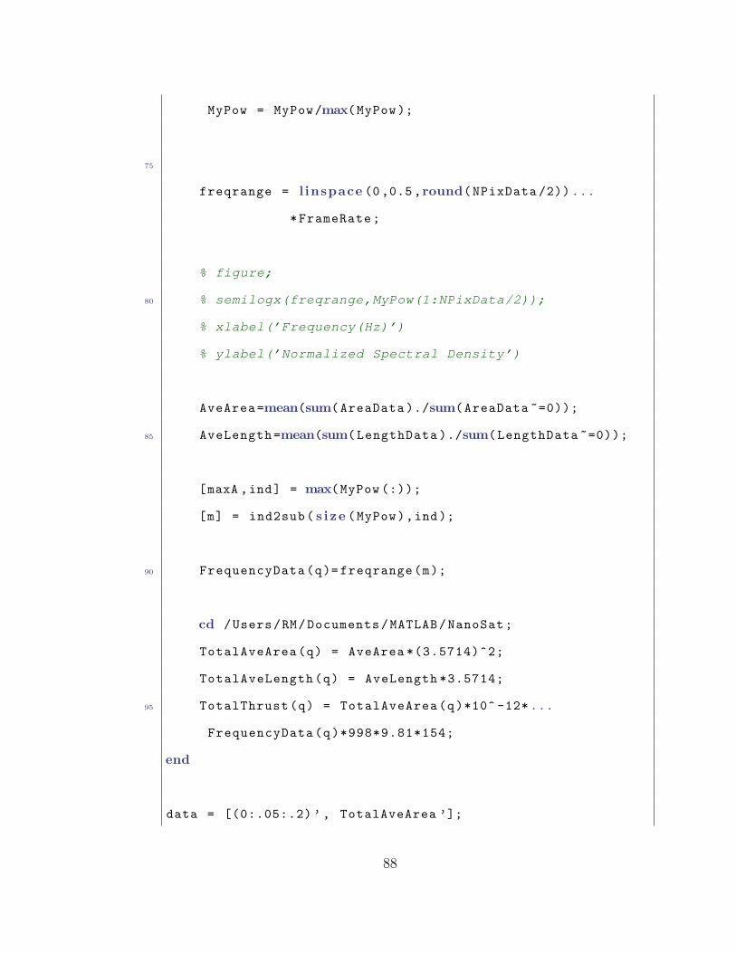
MyPow = MyPow/max(MyPow);
75
freqrange = l inspace (0,0.5,round(NPixData /2)) ...
*FrameRate;
% figure;
80 % semilogx(freqrange,MyPow(1:NPixData/2));
% xlabel(’Frequency(Hz)’)
% ylabel(’Normalized Spectral Density’)
AveArea=mean(sum(AreaData )./sum(AreaData ~=0));
85 AveLength=mean(sum(LengthData )./sum(LengthData ~=0));
[maxA ,ind] = max(MyPow (:));
[m] = ind2sub( s i ze (MyPow),ind);
90 FrequencyData(q)= freqrange(m);
cd /Users/RM/Documents/MATLAB/NanoSat;
TotalAveArea(q) = AveArea *(3.5714)^2;
TotalAveLength(q) = AveLength *3.5714;
95 TotalThrust(q) = TotalAveArea(q)*10^ -12* ...
FrequencyData(q)*998*9.81*154;
end
data = [(0:.05:.2) ’ , TotalAveArea ’];
88
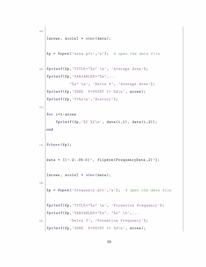
100
[nrows , ncols] = s i ze (data);
fp = fopen(’area.plt’,’w’); % open the data file
105 f p r in t f (fp ,’TITLE ="%s" \n’, ’Average Area’);
f p r in t f (fp ,’VARIABLES ="%s",...
"%s" \n’, ’Delta V’, ’Average Area’);
f p r in t f (fp ,’ZONE F=POINT I= %d\n’, nrows );
f p r in t f (fp ,’T=%s\n’,’History ’);
110
for i=1: nrows
f p r in t f (fp ,’%f %f\n’, data(i,1), data(i,2));
end
115 f c l o s e (fp);
data = [( -.2:.05:0) ’ , flipdim(FrequencyData ,2) ’];
[nrows , ncols] = s i ze (data);
120
fp = fopen(’frequency.plt’,’w’); % open the data file
f p r in t f (fp ,’TITLE ="%s" \n’, ’Formation Frequency ’);
f p r in t f (fp ,’VARIABLES ="%s", "%s" \n’,...
125 ’Delta V’, ’Formation Frequency ’);
f p r in t f (fp ,’ZONE F=POINT I= %d\n’, nrows );
89

f p r in t f (fp ,’T=%s\n’,’History ’);
for i=1: nrows
130 f p r in t f (fp ,’%f %f\n’, data(i,1), data(i,2));
end
f c l o se (fp);
135 data = [( -.2:.05:0) ’ , flipdim(TotalAveLength ,2) ’];
[nrows , ncols] = s i ze (data);
fp = fopen(’length.plt’,’w’); % open the data file
140
f p r in t f (fp ,’TITLE ="%s" \n’, ’Average Length ’);
f p r in t f (fp ,’VARIABLES ="%s", "%s" \n’,...
’Delta V’, ’Average Length ’);
f p r in t f (fp ,’ZONE F=POINT I= %d\n’, nrows );
145 f p r in t f (fp ,’T=%s\n’,’History ’);
for i=1: nrows
f p r in t f (fp ,’%f %f\n’, data(i,1), data(i,2));
end
150
f c l o s e (fp);
data = [(0:.05:.2) ’ , TotalThrust ’];
90
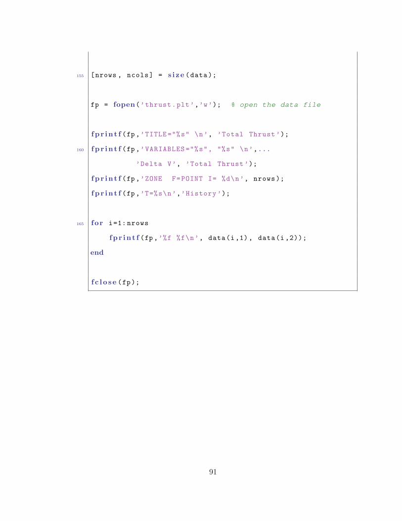
155 [nrows , ncols] = s i ze (data);
fp = fopen(’thrust.plt’,’w’); % open the data file
f p r in t f (fp ,’TITLE ="%s" \n’, ’Total Thrust ’);
160 f p r in t f (fp ,’VARIABLES ="%s", "%s" \n’,...
’Delta V’, ’Total Thrust ’);
f p r in t f (fp ,’ZONE F=POINT I= %d\n’, nrows );
f p r in t f (fp ,’T=%s\n’,’History ’);
165 for i=1: nrows
f p r in t f (fp ,’%f %f\n’, data(i,1), data(i,2));
end
f c l o se (fp);
91