Numerical studies of light-matter interaction driven by

plasmonic fields: the velocity gauge

A. Chacona, M. Lewensteina,b, M. F. Ciappinac

aICFO-Institut de Ciences Fotoniques, Av. Carl Friedrich Gauss 3, 08860 Castelldefels(Barcelona), Spain

bICREA-Institucio Catalana de Recerca i Estudis Avancats, Lluis Companys 23, 08010Barcelona, Spain

cMax-Planck-Institut fur Quantenoptik, Hans-Kopfermann-Str. 1, 85748 Garching,Germany

Abstract

Theoretical approaches to strong field phenomena driven by plasmonic fieldsare based on the length gauge formulation of the laser-matter coupling. Fromthe theoretical viewpoint it is known there exists no preferable gauge andconsequently the predictions and outcomes should be independent of thischoice. The use of the length gauge is mainly due to the fact that the quantityobtained from finite elements simulations of plasmonic fields is the plasmonicenhanced laser electric field rather than the laser vector potential. In thispaper we develop, from first principles, the velocity gauge formulation ofthe problem and we apply it to the high-order harmonic generation (HHG)in atoms. A comparison to the results obtained with the length gauge ismade. It is analytically and numerically demonstrated that both gaugesgive equivalent descriptions of the emitted HHG spectra resulting from theinteraction of a spatially inhomogeneous field and the single active electron(SAE) model of the helium atom. We discuss, however, advantages anddisadvantages of using different gauges in terms of numerical efficiency.

Keywords: Strong field phenomena, time dependent Schrodinger equation,plasmonic fields

1. Introduction

Nowadays there exists a high demand for coherent light sources extendingfrom the ultraviolet (UV) to the extreme ultraviolet (XUV) spectral ranges.

Preprint submitted to Journal of Computational Physics February 18, 2018

arX

iv:1

508.

0488

9v1

[ph

ysic

s.at

om-p

h] 2

0 A

ug 2

015

These sources provide important tools for basic research, material scienceand biology among other branches [1]. An important obstacle preventingthese sources from reaching high efficiency and large duty cycles is theirdemanding infrastructure. The recent demonstration of XUV generationdriven by surface plasmon resonances, conceived as light enhancers, couldprovide a plausible solution to this problem [2]. The high-order-harmonicgeneration (HHG) in atoms using plasmonics fields, generated starting fromtailored metal nanostructures, requires no extra amplification of the incomingpulse. By exploiting the so-called surface plasmon polaritons (SPP), thelocal electric fields can be enhanced by several orders of magnitude [2, 3, 4],thus exceeding the threshold laser intensity for HHG generation in noblegases. One additional advantage is that the pulse repetition rate remainsunaltered without any extra pumping or cavity attachment. Furthermore,the high-harmonics radiation, generated from each nanostructure typically inthe UV to XUV range, acts as a source with point-like properties, enablingcollimation or focusing of this coherent radiation by means of constructiveinterference. This opens a wide range of possibilities to spatially arrangenanostructures to enhance or shape the spectral and spatial properties of theoutgoing coherent radiation in numerous ways.

One can shortly describe the high-order-harmonic generation based onplasmonics fields as follows (a more exhaustive description can be found inthe seminal paper of Kim et al. [2]): a femtosecond low-intensity laser pulseis coupled to the plasmon mode of a metal nanostructure inducing a col-lective oscillation of the free electrons within the metal. These free chargesredistribute the electric field of the laser around each of the nanostructures,thereby forming a spot of highly enhanced electric field, also known as hotspot. The plasmon amplified field exceeds the threshold of HHG, thus byinjection of a gas jet, typically a noble gas, onto the spot of the enhancedfield, high order harmonics from the gas atoms are generated. In the originalexperiment of Kim et al. [2], the output laser beam emitted from a low-power femtosecond oscillator was directly focused onto a 10 × 10 µm sizearray of bow-tie nanoantennas with a pulse intensity of the order of 1011

W/cm2, which is about two orders of magnitude smaller than the thresholdintensity to generate HHG in noble gas atoms. The experimental result ofRef. [2] showed that the field intensity enhancement factor exceeded 20 dB,i.e. the enhanced laser intensity is two orders of magnitude larger than theinput one, which is enough to produce from the 7th to the 21st harmon-ics of the fundamental frequency by injecting xenon gas. For the case of

2

the laser wavelength corresponding to a Ti:Sa laser, i.e. about 800 nm, thewavelength of the emitted coherent radiation is between 38 nm and 114 nm.Additionally, each bow-tie nanostructure acts as a point-like source, thus athree-dimensional (3D) arrangement of bow-ties should enable us to performcontrol of the properties of generated harmonics, e.g. their polarization, invarious ways by exploiting interference effects. Due to the strong confinementof the plasmonic hot spots, which are of nanometer size, the laser electric fieldis clearly no longer spatially homogeneous in this tiny region. Since typicallyelectron excursions are of the same order as the size of this region, importantchanges in the laser-matter processes occur, see. e.g. [5, 6, 7].

So far, all of the the numerical approaches to study laser-matter processesin atoms and molecules driven by plasmonic fields, in particular HHG andATI, are based on the length gauge of the laser-coupling formulation [8, 9,10, 11, 12, 13, 14, 15, 16, 17, 18, 19, 20, 21, 22, 23, 25]. The use of the lengthgauge is mainly due to the fact that the quantity obtained from finite elementssimulations of plasmonic fields is the plasmonic enhanced laser electric fieldrather than the laser vector potential. Only a couple of papers employed anextension of the Strong Field Approximation (SFA), where an approximateversion of the velocity gauge was used [5, 16]. Different descriptions of lightmatter interaction (c.f. Ref. [28]), which include the full spatial dependenceof the electromagnetic field, are closely related to the problem presentedin our contribution. There are, however, distinct differences amongst thegeneral formulation of the non-dipole problem with the one we will tackle inthe present article. For instance, the next order of the non-dipole descriptionincludes both the electric quadrople and the magnetic dipole terms, whichare not present in our plasmonic fields, because the typical laser intensitiesare far below the ones needed to consider relevant these effects.

In this article, we concentrate our effort on the formulation and numericalimplementation of the velocity gauge description of light-matter interactiondriven by plasmonic fields. From a pure theoretical viewpoint, it is knownthe velocity gauge is more appropriate and consequently our contributionwill fill the missing gap, completing the whole picture in the modeling oflaser-matter processes driven by plasmonic fields.

The paper is organized as follows. In Sec. II, we shall present the velocitygauge formulation of the problem and we relate it to the length gauge, clearlyshowing the compatibility between them. The numerical implementation ispresented in Sec. III, joint with a set of examples and a discussion about howthe two different algorithms, i.e. the spectra split operator and the Crank-

3

Nicolson, behave as a function of the relevant parameters. Furthermore ananalysis of the computational efficiency and scaling of both formulations ispresented here. The paper ends with a short summary and an outlook.

2. Theory and gauge transformation

Quantum mechanics governs the evolution of the systems, atoms andmolecules in our case, when they interact with an extental electromagneticfield. In particular, the Time Dependent Schrodinger Equation (TDSE) [33]allows us to obtain the complete time-space evolution of the particles. Froma mathematical viewpoint, there are two different, but equivalent, expres-sions for the Hamiltonian which describes the interactions of the whole sys-tem. As a consequence the laser-matter problem can be formulated both inthe so called velocity gauge (VG) or in the length gauge (LG), indistinctly.Formally, both gauges present equivalent descriptions of the quantum prob-lem [33], and therefore the results should not change if either the VG or LGis utilized to compute the observables of interest. Here, we detail how thegauge transformation is commonly implemented in the laser-matter interac-tion and in particularly when a spatial inhomogeneous field interacts withan atomic or molecular target. In general, we are interested in to describethe electron dynamics of an atomic or molecular system when it interactswith an electromagnetic field. For this case the TDSE reads (atomic unitsare used throughout the paper otherwise stated):

HΨ(r, t) = i∂

∂tΨ(r, t), (1)

where, H, is the Hamiltonian of the quantum system and Ψ(r, t) is the elec-tron wavefunction (EWF).

Let us define the Hamiltonian, HV, in the minimum coupling or VG forthe electromagnetic field-matter interaction as:

HV =1

2[p + A(r, t)]2 + V0(r), (2)

where, p = −i∇, denotes the canonical momentum operator, A(r, t), is thevector potential of the electromagnetic field, which in this case correspondsto a spatial inhomogeneous or plasmonic field. In Eq. (2), V0(r, t) is theelectrostatic Coulomb interaction between the charged particles. The vector

4

potential for the spatial inhomogeneous field typically can be represented inthe following form:

A(r, t) = [1 + εg(r)]Ah(t),

Ah(t) = A0f(t) sin(ω0t+ ϕCEP)ez. (3)

Here, Ah(t), denotes the homogeneous or conventional vector potential, A0

is the amplitude of the vector potential, ω0, is the central frequency, ϕCEP

is the carrier-envelope-phase (CEP) and f(t) is a function which defines thetime envelope of the field. ε is a small parameter that governs the strength ofthe spatial inhomogeneity (see e.g. [5] for more details) and g(r) describe thespatial dependence of the plasmonic field. Note that in the limit when ε = 0,the vector potential field does not depend on the spatial coordinate anymoreand we recover the conventional laser-matter formulation. The units of εdepend on the function g(r). For instance, if g(r) = z (a linear function), εhas units of inverse length (see e.g. [5]).

Often, it is desirable to solve the TDSE in the length gauge or the maximalcoupling gauge. This is so because the numerical or analytical calculationcan be expressed in an easy way and the computation of certain observablesis more efficient [29]. Therefore, the main question is how we can performthe transformation of the Hamiltonian in the VG, Eq. (2), to the LG. Thegauge transformation should be boiling down in an unitary translation of thewhole wavefunction [24]. We define this unitary transformation according to:

ΨV = Q†ΨL, (4)

where, ΨV = ΨV(r, t) and ΨL = ΨL(r, t) are the wavefunctions in the VGand LG, respectively. Q is the unitary hermitian operator defined accordingto the following rule Q = exp [iχ(r, t)] [24, 32, 33], with χ(r, t) =

∫ r

CA(r′, t) ·

dr′. The latter expression is a contour integral which is independent of thepath, because we can safely assume that the effect of the magnetic field isnegligible, i.e. that the curl of the vector potential for the inhomogeneousfield is zero, ∇×A = 0. Furthermore, by using Eqs. (1) and (4), we find thetransformation for the Hamiltonian, HV, from the VG to the LG:

QHVQ†ΨL =

∂χ(r, t)

∂tΨL + i

∂ΨL

∂t. (5)

Then, knowing that E(r, t) = − ∂∂tA(r, t), i.e. the relationship between

5

E(r, t) and A(r,t), the last expression becomes:[QHVQ

† +

∫ r

C

E(r′, t) · dr′]

ΨL = i∂ΨL

∂t. (6)

As the TDSE is gauge invariant, we infer that the Hamiltonian in the VG,HV, is transformed to the LG, HL, via:

HL = QHVQ† +

∫ r

C

E(r′, t) · dr′. (7)

It can be demonstrated that the first term on the right hand side of Eq. (7),yields QHVQ

† = 12p2 + V0(r). Then, the Hamiltonian in the LG takes the

form:

HL =p2

2+ V0(r) + Vint(r, t), (8)

here, p is the kinetic momentum operator, and Vint(r, t) =∫ r

CE(r′, t) · dr′,

is a contour integral. In terms of Classical Mechanics, we can interpret thislast term as the work done in the electric field E(r′, t) to move the electronfrom an arbitrary place to the position r. In the particular case when thevector potential has the functional form given by Eq. (3) and the functiong(r), is set to g(r) = z, the Hamiltonian operator in the LG becomes:

HL =p2

2+ V0(r) + z(1 +

ε

2z)Eh(t), (9)

where, Eh(t) = − ∂∂tAh(t) denotes the spatial homogeneous part of the laser

electric field. Commonly this field, Eh(t), is called the conventional or spatialhomogeneous field.

In the next section, we shall compare the numerical accuracy of the VGand LG predictions for the high-order harmonic generation (HHG) driven byplasmonic fields. Our numerical models are based on Eqs. (2), for the VG,and (9), for the LG, respectively.

3. Numerical algorithms

The methods utilized to numerically integrate the TDSE are classifiedby considering how the time evolution of the EWF is computed. When theEWF at a later time is obtained from the one at the current time, we have

6

the so-called explicit methods. On the other hand, implicit schemes findthe EWF by solving an equation involving both the actual EWF and oneat later time. We choose the Spectral-Split Operator (SO) method jointwith the Crank-Nicolson (CN) scheme, which are both explicit methods, tonumerically integrate the TDSE of our interest. The SO uses a spectraltechnique to evaluate the derivative operator in the Fourier domain [31, 34],and, on the other hand, the CN is based on the finite element differencediscretization technique [34] to implement the second derivative present inthe Hamiltonian, which defines the kinetic operator term.In order to test the accuracy of both the VG and the LG in the HHG drivenby plasmonic fields, we have implemented the TDSE via the SO and CNtechniques within a one spatial dimension model (1D).A general solution of the TDSE is done by employing a unitary U(t0 +∆t, t0)evolution operator, where t0 is the initial time, i.e. the initial EWF Ψ0(t0) isknown and we evolve the system to an unknown state Ψ(t0 + ∆t) at a giventime t0 + ∆t [33]:

Ψ(t0 + ∆t) = U(t0 + ∆t, t0)Ψ0(t0). (10)

For simplicity, in Eq. (10), we have dropped out the spatial (r) dependenceon the EWF. In the laser-matter community, the U(t0 + ∆t, t0) is commonlyknown as a propagator and it has the following explicit form, U(t0 +∆t, t0) =

exp[−i∫ t0+∆t

t0H(t′)dt′

].

In reference [31], Feit et al. have introduced the SO method to numericallysolve the TDSE in two spatial dimensions (2D) by using Eq. (10). Thismethod consists in to split the time evolution operator U(t0 + ∆t, t0) ≈e−iH(t0+ ∆t

2)∆t in three parts [31]:

Ψ(t0 + ∆t) = e−i12p2∆t/2e−iVeff(t0+ ∆t

2)∆te−i

12p2∆t/2Ψ0(t0). (11)

Here, the Hamiltonian, H(t0 + ∆t2

), is divided in H(t0 + ∆t2

) = 12p2 +Veff(t0 +

∆t2

), with Veff(t) = V0(r)+∫ r

CE(r′, t)·dr′ the effective potential in the LG. The

main advantage of Eq. (11) is that we can evaluate the kinetic operator term,

e−i12p2∆t/2Ψ0(r, t0), acting on the initial state, in the momentum space. This

means that we need to compute a Forward Fourier Transform (FFT) [26] ofΨ0(r, t0) and then multiply it by a phase factor which evaluates the action ofthe kinetic operator, instead of a complicated derivate operator. Then, overthis momentum space EWF, an Inverse Fourier Transform (IFT) is applied

7

in order to return to the coordinate space [31]. This procedure is performedbecause the momentum operator in the conjugate (momentum) space is justa number and not a derivative one.For the conventional or homogeneous fields case, the vector potential doesnot depend on the spatial coordinate, i.e. A(r, t) = A(t), allowing us toevaluate the kinetic operator in the VG as:

Ψ(t0 + ∆t) = e−i12

(p+A(t0+∆t/2))2∆t/2e−iV0∆te−i12

(p+A(t0+∆t/2))2∆t/2Ψ0(t0). (12)

Clearly, this is not the case for the spatial nonhomogeneous fields. Thedependence of the vector potential on the position, as stated in Eq. (3), doesnot allow us to apply Eq. (12). This is so because in the momentum spacethe position operator becomes a derivative, which complicates substantiallythe SO method. Therefore, we conclude that the SO method can not beeasily employed to numerically integrate the TDSE in the VG. However, byusing a finite element grid discretization, we will show that the CN methodcan be used in both gauges, VG and LG. The CN method is based on thesolution of Eq. (10) by the Caley formula and the evaluation of the kineticoperator in the position space using a finite element method [34]. In 1D thenumerical algorithm can be written as:[

1 + i∆t

2H(t0 + ∆t/2)

]Ψ(t0 + ∆t) =

[1− i∆t

2H(t0 + ∆t/2)

]Ψ0(t0). (13)

The unknown EWF, Ψ(t0 + ∆t), is then computed by solving a tridiagonalsystem of equations.

4. System description and results

In Attosecond Science, high-order harmonic generation (HHG) is oneof the most important phenomena. For instance, it is possible to synthe-size attosecond pulses or to obtain structural information about the atomicof molecular systems [1] from the HHG spectra. Therefore, we chose herethis observable driven by conventional (homogeneous) and non-homogeneousfields to compare the accuracy of our VG and LG implementations.

For simplicity, we restrict ourselves to a one dimensional (1D) model,although it is known this approach is able to accurately reproduce the mainfeatures of the HHG spectra of real atoms [36]. The potential well, V0(x),

8

which defines our atomic system, is a soft-core or quasi Coulomb potential:

V0(x) = − Z√x2 + a

, (14)

where Z is the atomic charge and a a parameter which allows us to tune theionization potential of the atom of interest. In this paper, we set Z = 1 anda = 0.488 a.u., such as the ionization potential is Ip = 0.9 a.u. (24.6 eV), i.ethe value for the single active electron (SAE) model of the He atom [27]. Ourground state was computed via imaginary time propagation for a differentset of spatial grid steps δx. To assure a “good time” step, δt, convergence,we have used the criterion: δt < δx2/2 (for more details see e.g. [34]).

In order to compute the HHG spectra, we firstly calculate the dipoleacceleration expectation value, ad(t), as a function of time:

ad(t) = 〈Ψ(t)|∂V0(x)

∂x+ E(x, t)|Ψ(t)〉, (15)

where the EWF Ψ(x, t) is obtained via the SO and CN methods alreadydescribed in the previous Section. The spectral intensity, IHHG(ω) = |ad(ω)|2,of the harmonic emission is then computed by Fourier transforming the dipoleacceleration by using:

ad(ω) =

∫ +∞

−∞dt′ad(t

′)eiωt′. (16)

The numerical computation of the HHG spectra will be performed by using aset of position steps δx = {0.05, 0.1, 0.15, ...} a.u. Consequently, and in orderto estimate the numerical convergence of the HHG spectra as a function of δx,we use the spectral intensity difference between the smallest step, i.e. δx0 =0.05 a.u., and the rest of the set, ∆IHHG,δxj

(ω) = |IHHG,δx0(ω)− IHHG,δxj(ω)|,

with j = {1, 2, ...}. Furthermore, for each of the δx, the computing time isalso retrieved for both the VG and LG.

4.1. HHG driven by conventional fields

Firstly, we present computations of the harmonic spectra intensity, IHHG(ω),driven by a conventional homogeneous field. This case is the limit ε → 0.Both numerical methods above described, i.e. the SO and CN, have beenused to compute the emitted harmonic spectra intensity both in the VG andLG. We shall show below that both gauges give the same results.

9

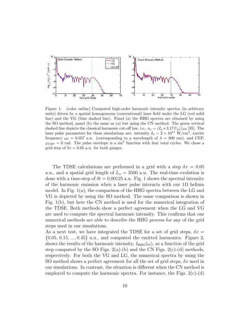
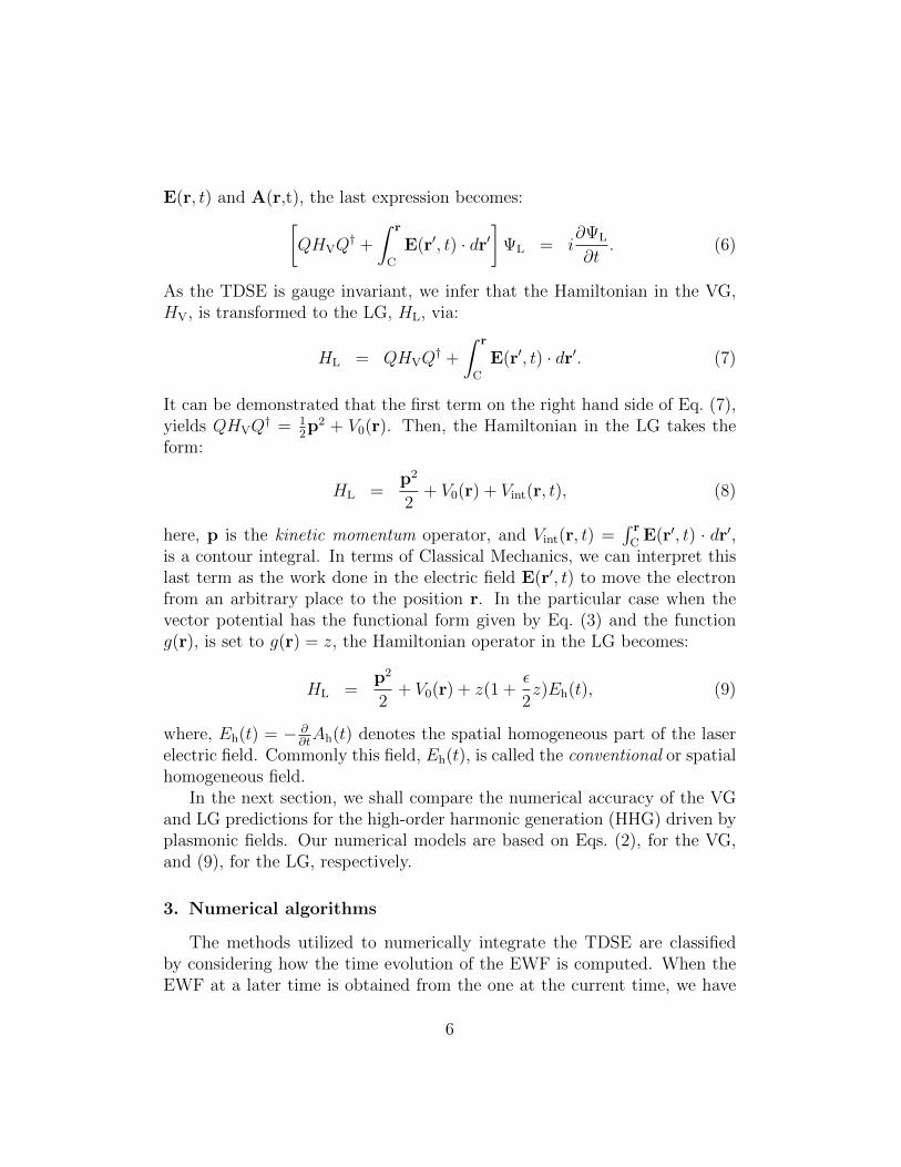
Figure 1: (color online) Computed high-order harmonic intensity spectra (in arbitraryunits) driven by a spatial homogeneous (conventional) laser field under the LG (red solidline) and the VG (blue dashed line). Panel (a) the HHG spectra are obtained by usingthe SO method, panel (b) the same as (a) but using the CN method. The green verticaldashed line depicts the classical harmonic cut-off law, i.e., nc = (Ip+3.17Up)/ω0 [35]. Thelaser pulse parameters for these simulations are: intensity I0 = 2 × 1014 W/cm2, carrierfrequency ω0 = 0.057 a.u. (corresponding to a wavelength of λ = 800 nm), and CEP,ϕCEP = 0 rad. The pulse envelope is a sin2 function with four total cycles. We chose agrid step of δx = 0.05 a.u. for both gauges.

The TDSE calculations are performed in a grid with a step δx = 0.05a.u., and a spatial grid length of Lx = 3500 a.u. The real-time evolution isdone with a time-step of δt = 0.00125 a.u. Fig. 1 shows the spectral intensityof the harmonic emission when a laser pulse interacts with our 1D heliummodel. In Fig. 1(a), the comparison of the HHG spectra between the LG andVG is depicted by using the SO method. The same comparison is shown inFig. 1(b), but here the CN method is used for the numerical integration ofthe TDSE. Both methods show a perfect agreement when the LG and VGare used to compute the spectral harmonic intensity. This confirms that ournumerical methods are able to describe the HHG process for any of the gridsteps used in our simulations.As a next test, we have integrated the TDSE for a set of grid steps, δx ={0.05, 0.15, ..., 0.45} a.u., and computed the emitted harmonics. Figure 2,shows the results of the harmonic intensity, IHHG(ω), as a function of the gridstep computed by the SO Figs. 2(a)-(b) and the CN Figs. 2(c)-(d) methods,respectively. For both the VG and LG, the numerical spectra by using theSO method shows a perfect agreement for all the set of grid steps, δx used inour simulations. In contrast, the situation is different when the CN method isemployed to compute the harmonic spectra. For instance, the Figs. 2(c)-(d)

10

Figure 2: (color online) Computed high-order harmonic intensity spectra driven by aspatial homogeneous (conventional) field (in arbitrary units) as a function of the gridstep, δx, under the LG and the VG by the SO method, panels (a)-(b) and the CN methodpanels (c)-(d). The green vertical dashed line depicts the classical harmonic cut-off law.The laser pulse parameters for these simulations are the same as in Fig. 1, i.e. intensityI0 = 2 × 1014 W/cm2, carrier frequency ω0 = 0.057 a.u. (corresponding to a wavelengthof λ = 800 nm), and CEP, ϕCEP = 0 rad. The pulse envelope is a sin2 function with fourtotal cycles.

11

show that the emitted harmonic spectrum depends on the grid step when theLG and VG are employed to computed the HHG. In addition, the computedHHG spectra slightly differ in the whole harmonic-order range whether theLG or the VG is used in the calculation and for the larger grid steps, i.e., δx ≥0.25 a.u. Additional structures can be observed in the low-order harmonicsfor the case of VG (see Figs. 2(d)), although the general shape, includingthe harmonic cutoff, is in excellent agreement with the rest of the schemes.Considering the numerical error that the finite element method has for thesecond derivative as a function of the grid spacing δx, it is reasonable toattribute poor convergence when the CN method is used with larger gridsteps δx. Furthermore, in view of the fact that the VG has an extra spatialderivative of first order within the Hamiltonian, p ·A, we would expect thatthe numerical accuracy decreases when the spatial step, δx, increases. This isthe reason behind the noticeable difference between the LG and the VG whenlarger grid steps are employed in the calculations of the HHG. Our numericalresults show, however, that this difference between LG and VG disappearsfor the smallest spatial grid steps, i.e., δx ≤ 0.2 a.u. These outcomes suggestthat the best method to compute the HHG spectrum is the SO. On the otherhand, in cases where the SO method is challenging, the CN method can beused if the grid step is small enough, e.g. δx . 0.1 a.u. We should note thatthe grid step will depend on the particular problem, i.e. laser parameters,etc., although we can expect a general trend. For this reason, we suggest toperform a convergence analysis if the CN method is employed and to chosethe adequate parameters for the required accuracy.

In the next, we shall perform the computation of the HHG spectra drivenby a spatial inhomogeneous field. For the reasons explained in Section 3, weshall only use the CN method and compute the harmonic emission both inthe LG and VG.

4.2. HHG driven by spatial inhomogeneous fields

As was mentioned at the outset, when a laser field is focused on a metal-lic nanostructure, a hot spot of higher intensity, high enough to exceed thethreshold for HHG in atoms, is created due to the coupling between the in-coming field and the surface plasmon polaritons (SPPs) [2]. The main prop-erty of the effective laser electric field is that it presents a spatial variation inthe same scale as the one of the dynamics of the active electron. Therefore,the interaction between this plamonic field and the atomic electron, whichgoverns the HHG process, will change substantially. As the electric field is

12

0 50 100 150 200 250−10

−8

−6

−4

−2

0

2

Harmonic−order

log

10[|a

d(ω

)|2]

LG

VG ε= 0.0175 a.u.

Figure 3: (color online) HHG spectra driven by a spatial inhomogeneous field computedby using the LG (blue line) and VG (red dashed line). The parameters for the laser pulseare the same that those used in Fig. 2, the inhomogeneous parameter is ε = 0.0175 a.u.(see the text for more details) and the grid step is δx = 0.05 a.u.

not anymore spatially homogeneous, the electron will experience differentelectric field strengths along its trajectory. The question that emerges iswhich gauge can give us a numerical advantage when the TDSE is solved forthe computation of the HHG spectra driven by spatial inhomogeneous fields.Before to address this question, we firstly demonstrate that both the LG andVG are equivalent in the description of the HHG driven by nonhomogeneousfields, as was demonstrated by the conventional case (see Section 4.1).We have numerically integrated the TDSE in 1D for the same atomic sys-tem used in the previous section (Section 4.1), but now the effective electricfield is spatially inhomogeneous. Fig. 3 shows the comparison between thecalculated HHG spectra driven by an inhomogeneous field for both the LGand VG. The inhomogeneous parameter value is set at ε = 0.0175 a.u., whichcorrespond to an inhomogeneous region of about 60 a.u. (3 nm) (see [5] formore details). Perfect agreement between the predictions of both the LGand VG are found. Therefore, these results suggest that our derivations areappropriate for spatial nonhomogeneous fields as well. As a consequence,this invariance allows us to check which gauge can be more convenient tocompute the HHG driven by spatial nonhomogeneous fields. We will addressthis point by considering the convergence of both the LG and VG. In otherwords, which of the two gauges presents less numerical error against the grid

13

Figure 4: (color online) HHG spectra driven by plasmonic fields both in the LG andVG as a function of the grid step δx are depicted in panel (a) and (b), respectively. Wehave used the CN method to numerically integrate the TDSE. The parameters for thelaser pulse are the same that those used in Fig. 3 and the inhomogeneous parameter isε = 0.0175 a.u.

step, δx, and which one is faster in the computation of the HHG spectra.Fig. 4 shows the HHG spectra as a function of the grid step for both theLG Fig. 4(a) and the VG Fig. 4(b) computed by using the CN method. TheHHG spectra for the LG show a convergence for the smallest grid step, i.e.,for δx = 0.05 a.u. We should note, however, that the highest frequencyof the HHG spectra change when the grid step is increases, which suggeststhat the computation of the HHG spectra driven by spatial inhomogeneousfields deserves special attention when“large” grid steps are used. A similarresult is found when the VG is employed although it is possible to observeconvergence for larger values of δx. A suitable way to confirm the HHGcutoff and corroborate the convergence of the numerical schemes, is to rely onclassical simulations. It is known that the limits on the HHG spectra can beobtained via classical simulations, e.g. by computing the maximum electronkinetic energy upon recombination [35]. For spatial nonhomogeneous fields,it was demonstrated a perfect agreement between the classical predictionsand the TDSE simulations (see e.g. [5]) and, as a consequence, we couldbenchmark our VG and LG approaches by solving the classical equations ofmotion for an electron moving in an oscillating and spatial dependent electricfield (for more details see [23]).

In addition, despite of the fact that for larger grid steps the LG showsa large deviation for the highest frequency compared to the VG results, we

evaluate the relative error defined by∆IHHG,δxj

IHHG,δx0for each gauge as a function

14

a) b)

Figure 5: (color online) (a) Convergence relative-error as a function of the grid step byusing the LG (blue line with squares) and the VG (red line with circles). (b) computingreal-time as a function of the grid step for both the LG (blue squares) and VG (red circles).The simulation parameters are the same that those used in Fig. 4.

of the grid step δx. The results are depicted in Fig. 5(a). This panel showsthat a large difference appears whether LG or VG is used to compute theHHG spectra by the CN method. For values of δx larger than 0.2 a.u., therelative error between the LG and the VG has a difference of about twoorders of magnitude, which suggests that the LG would be more appropriatethan the VG to compute the HHG spectra. Finally, in the panel (b), we showthe computational time for each gauge. As can be observed the computingtimes for both the LG and the VG are similar. From this consideration wecan conclude that the LG could be the most appropriated gauge in order tocompute the HHG, given the fact it allows us to use larger grid steps.

5. Conclusions

We have reviewed the gauge invariance problem, both analytical and nu-merically, for the calculation of the HHG phenomenon driven by spatial ho-mogeneous and inhomogeneous (plasmonic enhanced) electric fields. To thispurpose we have solved the TDSE in reduced dimensions by implementingthe Spectral-Split Operator and the Crank-Nicolson algorithms. It was foundthat both the LG and VG are equivalent in the description of the harmonicemission processes for each of the two studied cases: the spatial homogeneousand the spatial inhomogeneous fields. For the spatial inhomogeneous fieldcase, and due to the dependence of the vector potential on the position, wefound that the SO method was difficult to implement in the numerical solu-

15

tion of the TDSE. In contrast, the CN method has shown advantages becauseit is based on a finite element discretization. Our numerical results based onthe CN method suggested that the calculation of the harmonic spectra de-pends strongly on the grid step chosen to perform the numerical integration.Both gauges are equivalent, but according to the numerical convergence ofthe HHG spectra, the LG apparently appears to be more accurate than theVG for the lowest harmonics. This is so because the lowest harmonics changeby several orders of magnitude when the grid step increases. Furthermore,it was shown that particular attention in the choice of the spatial grid stepshould to be taken when spatial inhomogeneous fields are employed. This isso, because the limits of the harmonic radiation appear to be very sensitiveto this parameter. Finally, it was found that the computational time wassimilar for both the LG or VG, if they were used for the computation of theHHG spectrum in the moderate and high laser intensity regimes.

6. Acknowledgments

We are grateful to Alejandro De La Calle for the insightful discussionand useful suggestions. A.C. and M.L. thanks the Spanish Ministry ProjectFrOntiers of QUantum Sciences (FOQUS, FIS2013-46768-P) and ERC AdGOSYRIS for financial support.

We also acknowledge the support from the ERCs Seventh Framework Pro-gramme LASERLAB-EUROPE III (grant agreement 284464) and the Min-isterio de Economıa y Competitividad of Spain (FURIAM project FIS2013-47741-R).

References

[1] F. Krausz, and M. Ivanov, Rev. Mod. Phys. 81 (2009) 163.

[2] S. Kim, J. Jin, Y.-J. Kim, I.-Y. Park, Y. Kim, and S.-W. Kim, Nature(London) 453 (2008) 757.

[3] I.-Y. Park, S. Kim, J. Choi, D.-H. Lee, Y.-J. Kim, M. F. Kling, M. I.Stockman, and S.-W. Kim, Nat. Phot. 5 (2011) 677.

[4] N. Pfullmann, C. Waltermann, M. Noack, S. Rausch, T. Nagy, M.Kovacev, V. Knittel, R. Bratschitsch, D. Akemeier, A. Hutten, A. Leit-enstorfer, and U. Morgner, New J. Phys. 15 (2013) 093027.

16

[5] M. F. Ciappina, J. Biegert, R.Quidant, and M. Lewenstein, Phys. Rev.A 85 (2012) 033828.

[6] M. F. Ciappina, S. S. Acimovic, T. Shaaran, J. Biegert, R. Quidant, andM. Lewenstein, Opt. Express 20 (2012) 26261.

[7] J. A. Perez-Hernandez, M. F. Ciappina, M. Lewenstein, L. Roso, andA. Zaır, Phys. Rev. Lett. 110 (2013) 053001.

[8] A. Husakou, S.-J. Im, and J. Herrmann, Phys. Rev. A 83 (2011) 043839.

[9] I. Yavuz, E. A. Bleda, Z. Altun, and T. Topcu, Phys. Rev. A 85 (2012)013416.

[10] T. Shaaran, M. F. Ciappina, and M. Lewenstein, Phys. Rev. A 86 (2012)023408.

[11] M. F. Ciappina, J. A. Perez-Hernandez, T. Shaaran, J. Biegert, R.Quidant, and M. Lewenstein, Phys. Rev. A 86 (2012) 023413.

[12] T. Shaaran, M. F. Ciappina, and M. Lewenstein, J. Mod. Opt. 59 (2012)1634.

[13] T. Shaaran, M. F. Ciappina, and M. Lewenstein, Ann. Phys. (Berlin)525 (2013) 97.

[14] B. Fetic, K. Kalajdzic, and D. B.Milosevic, Ann. Phys. (Berlin) 525(2013) 107.

[15] T. Shaaran, M. F. Ciappina, R. Guichard, J. A. Perez-Hernandez, L.Roso, M. Arnold, T. Siegel, A. Zaır, and M. Lewenstein, Phys. Rev. A87 (2013) 041402.

[16] T. Shaaran, M. F. Ciappina, and M. Lewenstein, Phys. Rev. A 87 (2013)053415.

[17] I. Yavuz, Phys. Rev. A 87 (2013) 053815.

[18] M. F. Ciappina, J. A. Perez-Hernandez, T. Shaaran, L. Roso, and M.Lewenstein, Phys. Rev. A 87 (2013) 063833.

[19] J. Luo, Y. Li, Z. Wang, Q. Zhang, and P. Lu, J. Phys. B 46 (2013)145602.

17

[20] M. F. Ciappina, T. Shaaran, R. Guichard, J. A. Perez-Hernandez, L.Roso, M. Arnold, T. Siegel, A. Zaır, and M. Lewenstein, Laser Phys.Lett. 10 (2013) 105302.

[21] M. F. Ciappina, J. A. Perez-Hernandez, T. Shaaran, M. Lewenstein, M.Kruger, and P. Hommelhoff, Phys. Rev. A 89 (2014) 013409.

[22] L. Q. Feng, M. Yuan, and T. Chu, Phys. Plasmas 20 (2013) 122307.

[23] M. F. Ciappina, J. A. Perez-Hernandez, and M. Lewenstein, Comp.Phys. Comm. 185 (2014) 398.

[24] J. R. Ackerhalt and P. W. Milonni, J. Opt. Soc. Am. B 1 (1984) 116.

[25] M. F. Ciappina, J. A. Perez-Hernandez, L. Roso, A. Zaır, and M. Lewen-stein, J. Phys. Conf. Ser. 601 (2015) 012001.

[26] M. Frigo and S. G. Johnson, FFTW http://www.fftw.org/.

[27] National Institute of Standards and Technology (NIST), Com-putational Chemistry Comparison and Benchmark DataBase,http://cccbdb.nist.gov/.

[28] S. Selstø, and M. Forre, Phys. Rev. A 76 (2007) 023427.

[29] E. Cormier, and P. Lambropoulos, J. Phys. B 29 (1996) 1667.

[30] D. Bauer, D. B. Milosevic, and W. Becker, Phys. Rev. A 72 (2005)023415.

[31] M. D. Feit, J. A. Fleck, and A. Steiger. J. Comp. Phys., 47 (1982) 412.

[32] C. Cohen-Tannoudji, B. Diu, and C. Laloe, Quantum Mechanics (Her-mann/Wiley, Paris, 1977).

[33] J. J. Sakurai, Modern Quantum Mechanics, (Addison Wesley, 1994).

[34] W. H. Press, S. A. Teukolsky, W. T. Vetterling, and P. B. Flannery,Numerical Recipes in C: The Art of Scientic Computing, (CambridgeUniversity Press, 2002).

[35] M. Lewenstein, P. Balcou, M. Y. Ivanov, A. L’Huillier, and P. B.Corkum, Phys. Rev. A 49 (1994) 2117.

18

[36] M. Protopapas, C. H. Keitel, and P. L. Knight, Rep. Prog. Phys. 60(1997) 389.

19