Embed Size (px)
Citation preview

Numerical Solutions of Numerical Solutions of Ordinary Differential Ordinary Differential
EquationsEquations
Numerical Solutions of Numerical Solutions of Ordinary Differential Ordinary Differential
EquationsEquations
1Dr.G.Suresh Kumar@KL University
04/19/23

Ordinary Differential Ordinary Differential EquationsEquations
Equations which are composed of an unknown function and its derivatives are called differential equations.
Differential equations play a fundamental role in engineering because many physical phenomena are best formulated mathematically in terms of their rate of change.
vm
cg
dt
dv
v - dependent variable
t - independent variable
04/19/23 2Dr.G.Suresh Kumar@KL University

Types of Differential Types of Differential EquationsEquations
• When a function involves one independent
variable, the equation is called an ordinary
differential equation (ODE).
•A partial differential equation (PDE)
involves two or more independent
variables.
04/19/23 3Dr.G.Suresh Kumar@KL University

Model Ordinary Differential Model Ordinary Differential EquationsEquations
04/19/23 4Dr.G.Suresh Kumar@KL University

Why Numerical solutions of Why Numerical solutions of ODE ?ODE ?
Many differential equations cannot be solved analytically, in which case we have to satisfy ourselves with an approximation to the solution.
04/19/23 Dr.G.Suresh Kumar@KL University 5

Initial value problemInitial value problem
Initial value problem associated with first order differential equations is
04/19/23 Dr.G.Suresh Kumar@KL University 6
.y)y(x
y)f(x,dx
dy
00

Methods of solving IVPMethods of solving IVPTaylor series Picard successive approximationEulerModified EulerRunge-Kutta (RK)
04/19/23 Dr.G.Suresh Kumar@KL University 7

Taylor Series MethodTaylor Series MethodThe Taylor series method is a
straight forward adaptation of classic calculus to develop the solution as an infinite series.
The method is not strictly a numerical method but it is used in conjunction with numerical schemes.
04/19/23 Dr.G.Suresh Kumar@KL University 8

Taylor Series MethodTaylor Series Method
The Taylor series expansion of y(x) about
x = x0 is
04/19/23 Dr.G.Suresh Kumar@KL University 9
...xy 4!
x-xxy
3!
x-x
xy 2!
x-xxy x-xxyxy
0(IV)
40
0
30
0
20
000
Problem#1Problem#1
The differential equation y'(x) = x + y satisfying y(0)=1. Determine the Taylor series solution. Also compare with the exact solution.
{Analytical solution: y(x)=2ex - x -1(Cauchy linear differential equation).}
04/19/23 Dr.G.Suresh Kumar@KL University 10

SolutionSolution
First, we find derivatives of y' = x + y,
04/19/23 Dr.G.Suresh Kumar@KL University 11
xyxy
xyxy
xy1xy
xyxxy
(IV)
2.0y0y
20y0y
2110y10y
1100yx0y
(IV)

SolutionSolutionThe Taylor series expansion of y(x)
about x = x0 is
04/19/23 Dr.G.Suresh Kumar@KL University 12
...xy 4!
x-xxy
3!
x-x
xy 2!
x-xxy x-xxyxy
0(IV)
40
0
30
0
20
000
... 12
x
3
x xx 1
... 2 4!
x2
3!
x2
2!
x1x 1xy
432
432

Comparison of solutionsComparison of solutions
The exact solution is
Therefore, Taylor series solution and exact solution are equal.
04/19/23 Dr.G.Suresh Kumar@KL University 13
...24
x
3
xxx1
1)(x...4!
x
3!
x
2!
xx12y(x)
432
432

Picard’s MethodPicard’s Method
04/19/23 Dr.G.Suresh Kumar@KL University 14
00 y)y(x
y)f(x,dx
dy
The initial value Problem
is equivalent to the following integral equation
.y(t))dtf(t,yy(x)x
x
0
0

Picard’s MethodPicard’s Method
04/19/23 Dr.G.Suresh Kumar@KL University 15
The Picard’s nth approximate solution is
... 3, 2, 1, n ,(t))dtyf(t,y(x)yx
x1n0n
0
.n as y(x)(x)yn

Problem#1Problem#1Using Picard’s process of successive
approximation, obtain a solution up to the fifth approximation of the equation
04/19/23 Dr.G.Suresh Kumar@KL University 16
y xdx
dy
such that y = 1 when x = 0. Check your answer by finding the exact solution.
720
x
60
x
12
x
3
xxx1(x)y
65432
5 Ans.
Exact solution y(x) = 2ex – (x+1).
Application ProblemApplication Problem
For the free-falling bungee jumper with linear drag, compute the velocity at 10 seconds of a free-falling parachutist of mass 80kg and drag coefficient 10 kg/s at 10 seconds, with initial velocity 20 m/s, using
(i) Taylor series method(ii) Picard’s method.
04/19/23 Dr.G.Suresh Kumar@KL University 17
SolutionSolutionLet v(t) be the velocity and ‘a’ be the
acceleration of the parachutist at any time t.
Then the total force acting on the parachutist is equal to the sum of the
downward force FD due to gravity andupward force FU due to air resistance.
i.e. F = FD + FU
FD = mg
FU α v (linear drag) FU = - Cd v(t).
04/19/23 Dr.G.Suresh Kumar@KL University 18

SolutionSolutionBy Newton second law of motion F =
ma.ma = mg – Cd v
Therefore,
04/19/23 Dr.G.Suresh Kumar@KL University 19
vm
Cg
dt
dv d
Given that m = 80kg, Cd = 10 kg/s,
and initial velocity v(0)=20 m/s.Now solve the above IVP using
Taylor and Picard’s method.

Euler’s MethodEuler’s Method
,...2,1),(
)(
:MethodEuler
,...2,1)(:Determine
)( :condition initial with the
),()(':ODEorder first Given the
:Problem
1
00
0
00
iforyxfhyy
xyy
iforihxyy
xyy
yxfxy
iiii
i
04/19/23 20Dr.G.Suresh Kumar@KL University
04/19/23 21
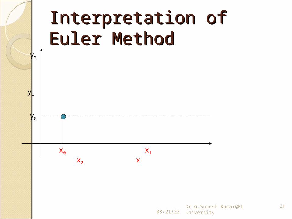
Interpretation of Euler Interpretation of Euler MethodMethod
x0 x1 x2 x
y0
y1
y2
Dr.G.Suresh Kumar@KL University

04/19/23 22
Interpretation of Euler Interpretation of Euler MethodMethod
hx0 x1 x2 x
y0
y1=y0+hf(x0,y0)
Slope=f(x0,y0)
hf(x0,y0)
y1
Dr.G.Suresh Kumar@KL University

04/19/23 23
Interpretation of Euler Interpretation of Euler MethodMethod
hx0 x1 x2 x
y0
y1=y0+hf(x0,y0)
Slope=f(x0,y0)
hf(x0,y0)y1
h
y2=y1+hf(x1,y1)Slope=f(x1,y1)
y2
hf(x1,y1)
Dr.G.Suresh Kumar@KL University
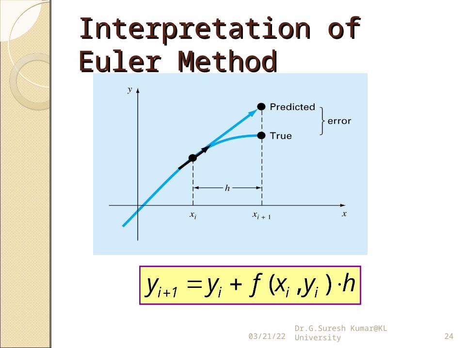
Interpretation of Euler Interpretation of Euler MethodMethod
04/19/23 Dr.G.Suresh Kumar@KL University 24

Problem#1Problem#1Using Euler’s method, find an
approximate value of y corresponding to x=1, given that yʹ = x + y such that y=1 when x=0.
Ans: Taking h = 0.1, theny(0.1) = 1.1, y(0.2) = 1.22, y(0.3) = 1.36y(0.4) = 1.53, y(0.5) = 1.72, y(0.6) =
1.94y(0.7) = 2.19, y(0.8) = 2.48, y(0.9) =
2.81y(1.0) = 3.18.
04/19/23 Dr.G.Suresh Kumar@KL University 25
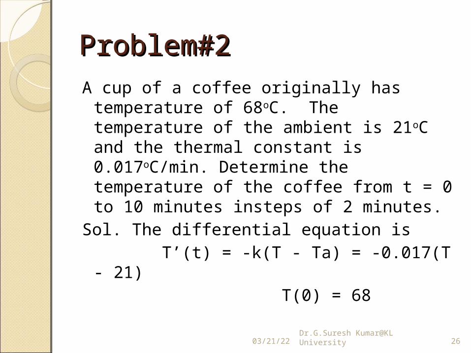
Problem#2Problem#2
A cup of a coffee originally has temperature of 68oC. The temperature of the ambient is 21oC and the thermal constant is 0.017oC/min. Determine the temperature of the coffee from t = 0 to 10 minutes insteps of 2 minutes.
Sol. The differential equation is Tʹ(t) = -k(T - Ta) = -0.017(T - 21) T(0) = 68
04/19/23 Dr.G.Suresh Kumar@KL University 26

Improvements of Euler’s methodImprovements of Euler’s methodA fundamental source of error in Euler’s
method is that the derivative at the beginning of the interval is assumed to apply across the entire interval.
Two simple modifications are available to circumvent this shortcoming:
Heun’s (Modified Euler) MethodMidpoint (Improved Polygon) Method
04/19/23 27Dr.G.Suresh Kumar@KL University

Modified Euler’s MethodModified Euler’s MethodTo improve the estimate of the slope, determine two
derivatives for the interval:(1) At the initial point(2) At the end pointThe two derivatives are then averaged to obtain an improved estimate of the slope for the entire interval.
hyxfyxf
yy
hyxfyy
iiiiii
iiii
2
),(),(:
),( :0
111
01
Corrector
Predictor
04/19/23 28Dr.G.Suresh Kumar@KL University

29
To improve the estimate of the slope, determine two derivatives for the interval:
At the initial point At the end point
The two derivatives are then averaged to obtain an improved estimate of the slope for the entire interval.
hyxfyxf
yy
hyxfyy
iiiiii
iiii
2
),(),(:
),( :0
111
01
Corrector
Predictor
Euler Modified methodEuler Modified method
30
hyxfyxf
yy
hyxfyy
iiiiii
iiii
2
),(),(:
),( :
0111
1
01
Corrector
Predictor
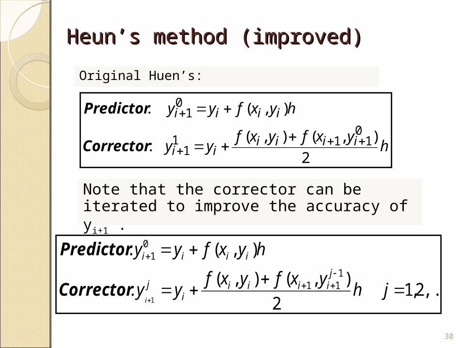
Heun’s method (improved)Heun’s method (improved)
,...2,1 2
),(),(:
),( :1
11
01
1
jh
yxfyxfyy
hyxfyyj
iiiii
j
iiii
iCorrector
Predictor
Note that the corrector can be iterated to improve the accuracy of yi+1 .
Original Huen’s:

Problem#1Problem#1Using Modified Euler’s method, find an
approximate value of y when x= 0.3, given that yʹ = x + y and y=1 when x=0.
Sol. Compare the IVP with the general IVP
yʹ = f(x, y), y(x0) = x0, we have
f(x, y) = x + y, x0 = 0 and y0 = 1.
Taking the step size h = 0.1, then x0 = 0, x1 = 0.1, x2 = 0.2, x3 = 0.3. Now we find the corresponding value of y, using modified Euler’s method.
31
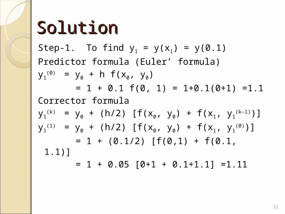
SolutionSolutionStep-1. To find y1 = y(x1) = y(0.1)
Predictor formula (Euler’ formula)y1
(0) = y0 + h f(x0, y0)
= 1 + 0.1 f(0, 1) = 1+0.1(0+1) =1.1Corrector formula y1
(k) = y0 + (h/2) [f(x0, y0) + f(x1, y1(k-1))]
y1(1) = y0 + (h/2) [f(x0, y0) + f(x1, y1
(0))]
= 1 + (0.1/2) [f(0,1) + f(0.1, 1.1)] = 1 + 0.05 [0+1 + 0.1+1.1] =1.11
32

SolutionSolutiony1
(2) = y0 + (h/2) [f(x0, y0) + f(x1, y1(1))]
= 1 + (0.1/2) [f(0,1) + f(0.1, 1.11)] = 1 + 0.05 [0+1 + 0.1+1.11] =1.1105.y1
(3) = y0 + (h/2) [f(x0, y0) + f(x1, y1(2))]
= 1 + (0.1/2) [f(0,1) + f(0.1, 1.1105)] = 1 + 0.05 [0+1 + 0.1+1.1105] =1.1105.Therefore, y1
= 1.1105.
33
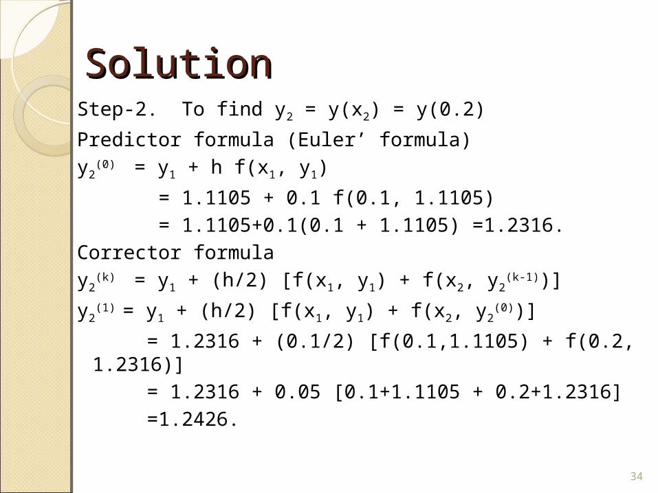
SolutionSolutionStep-2. To find y2 = y(x2) = y(0.2)
Predictor formula (Euler’ formula)y2
(0) = y1 + h f(x1, y1)
= 1.1105 + 0.1 f(0.1, 1.1105) = 1.1105+0.1(0.1 + 1.1105) =1.2316.Corrector formula y2
(k) = y1 + (h/2) [f(x1, y1) + f(x2, y2(k-1))]
y2(1) = y1 + (h/2) [f(x1, y1) + f(x2, y2
(0))]
= 1.2316 + (0.1/2) [f(0.1,1.1105) + f(0.2, 1.2316)] = 1.2316 + 0.05 [0.1+1.1105 + 0.2+1.2316] =1.2426.
34
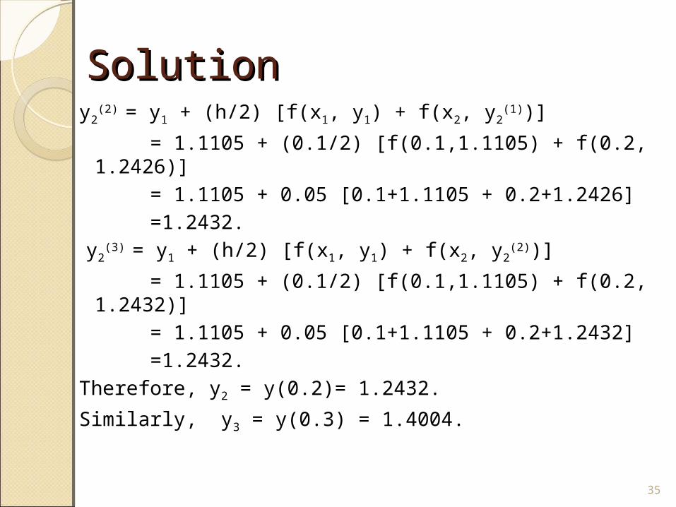
SolutionSolutiony2
(2) = y1 + (h/2) [f(x1, y1) + f(x2, y2(1))]
= 1.1105 + (0.1/2) [f(0.1,1.1105) + f(0.2, 1.2426)]
= 1.1105 + 0.05 [0.1+1.1105 + 0.2+1.2426] =1.2432. y2
(3) = y1 + (h/2) [f(x1, y1) + f(x2, y2(2))]
= 1.1105 + (0.1/2) [f(0.1,1.1105) + f(0.2, 1.2432)]
= 1.1105 + 0.05 [0.1+1.1105 + 0.2+1.2432] =1.2432.Therefore, y2 = y(0.2)= 1.2432.
Similarly, y3 = y(0.3) = 1.4004.35

Application ProblemApplication ProblemA storage tank (Fig.) contains a liquid
at depth y where y = 0 when the tank is half full. Liquid is withdrawn at a constant flow rate Q=500m3/h to meet demands. The contents are resupplied at a sinusoidal rate 3Q sin2(t). The surface area of the tank is 1200 m2. Determine the depth of the tank from t= 0 to t=6 in steps of 2 hours, using modified Euler’s method.
04/19/23 Dr.G.Suresh Kumar@KL University 36
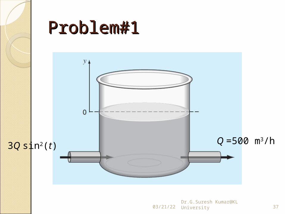
Problem#1Problem#1
04/19/23 Dr.G.Suresh Kumar@KL University 37
3Q sin2(t) Q =500 m3/h

SolutionSolutionLet y(t) be the depth of the tank at any time t
and A be the surface area of the tank.
The depth of the tank is changed when volume of the liquid in the tank changed. Therefore,
04/19/23 Dr.G.Suresh Kumar@KL University 38
rate flowout – rate inflow in volume
change of Rate
QQ (t)sin3Ay(t)dt
d 2
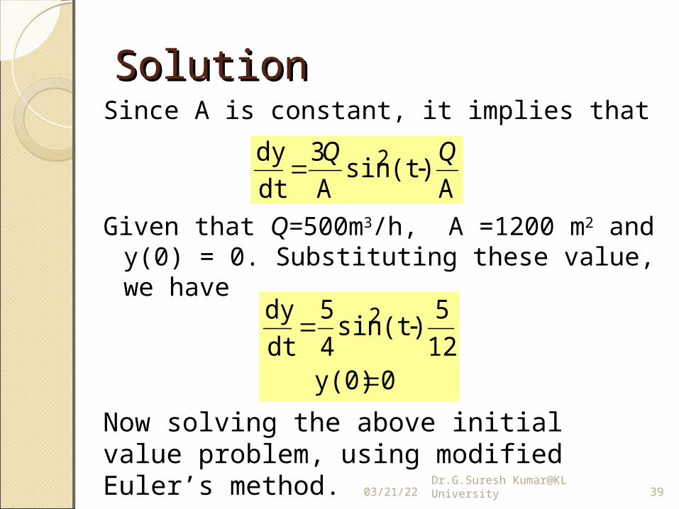
SolutionSolutionSince A is constant, it implies that
Given that Q=500m3/h, A =1200 m2 and y(0) = 0. Substituting these value, we have
04/19/23 Dr.G.Suresh Kumar@KL University 39
A(t)sin
A
3
dt
dy 2 QQ
0y(0) 12
5(t)sin
4
5
dt
dy 2
Now solving the above initial value problem, using modified Euler’s method.

Runge - Kutta Runge - Kutta MethodMethod
04/19/23 40Dr.G.Suresh Kumar@KL University

Carl RungeCarl Runge(1856-1927)(1856-1927)
Martin Wilhelm Kutta
(1867-1944)
04/19/23 41Dr.G.Suresh Kumar@KL University

IntroductionIntroductionRunge-Kutta methods are very popular because of
their good efficiency; and are used in most computer programs for differential equations.
These methods agree with Taylor’s series solution up to the term in hr, where r differs method to method and is called the order of the method.
Euler’s and modified Euler’s are called the first and second order Runge-Kutta methods.
The fourth order R-K method is most commonly used and is often referred to as R-K method only.
04/19/23 42Dr.G.Suresh Kumar@KL University

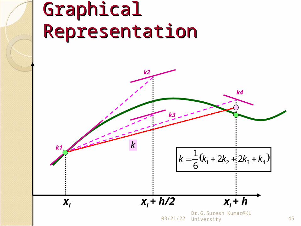
Working RuleWorking RuleTo find increment ‘k’ of y corresponding
to an increment h of x by R-K method from the initial value problem
y´ = f(x, y) with y(x0) = y0 is as follows
Calculate k1 = h f(x0, y0)
k2 = h f(x0+0.5h, y0+0.5k1)
k3 = h f(x0+0.5h, y0+0.5k2)
k4 = h f(x0+h, y0+k3)
04/19/23 43Dr.G.Suresh Kumar@KL University

Working RuleWorking RuleFinally compute k = 1/6 (k1 + 2k2 + 2k3 + k4)
is the weighted mean of k1, k2, k3 and k4.
Therefore the required approximate value is
y1 = y(x1) = y(x0 + h) = y0 + k.
04/19/23 44Dr.G.Suresh Kumar@KL University
Dr.G.Suresh Kumar@KL University
Graphical RepresentationGraphical Representation
xi xi + h/2 xi + h
k1
k2
k3
k4
4321 226
1kkkkk
k
04/19/23 45

Problem#1Problem#1Using Runge-Kutta method of
fourth order, solve yʹ = (y2 – x2)/(y2 + x2) with y(0)=1 at x = 0.2, 0.4.
Sol : - Compare the given problem with the general first order initial value problem yʹ=f(x, y) satisfying y(x0)=y0, we have
f(x, y) = (y2 – x2)/(y2 + x2) x0 = 0, y0 =1.
Here we have to find value of y at x=0.2, 0.4.04/19/23 46Dr.G.Suresh Kumar@KL University

SolutionSolutionTaking step size h = 0.2.Step(1) To find y(0.2) k1 = h f(x0, y0)
= 0.2 f(0, 1) = 0.2 (12-02)/(12+02) = 0.2 k2 = h f(x0+0.5h, y0+0.5k1)
= 0.2 f(0+0.5(0.2), 1+ 0.5(0.2)) = 0.2 f(0.1, 1.1) = 0.19672
04/19/23 Dr.G.Suresh Kumar@KL University 47
SolutionSolution
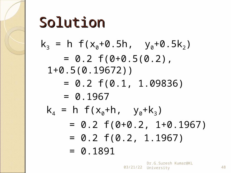
k3 = h f(x0+0.5h, y0+0.5k2)
= 0.2 f(0+0.5(0.2), 1+0.5(0.19672))
= 0.2 f(0.1, 1.09836) = 0.1967 k4 = h f(x0+h, y0+k3)
= 0.2 f(0+0.2, 1+0.1967) = 0.2 f(0.2, 1.1967) = 0.1891
04/19/23 Dr.G.Suresh Kumar@KL University 48

SolutionSolutionk = 1/6 (k1 + 2k2 + 2k3 + k4)
= 1/6 (0.2 +2(0.19672)+2(0.1967)+0.1891)
= 0.19599.Hence y1 = y0 + k
y(0.2) = 1 + 0.19599 = 1.19599.Step(2) To find y(0.4) k1 = h f(x1, y1)
= 0.2 f(0.2, 1.19599) = 0.1891
04/19/23 Dr.G.Suresh Kumar@KL University 49

solutionsolutionk2 = h f(x1+0.5h, y1+0.5k1)
= 0.2 f(0.2+0.5(0.2), 1.19599+ 0.5(0.1891)) = 0.2 f(0.3, 1.29054) = 0.1795k3 = h f(x1+0.5h, y1+0.5k2)
= 0.2 f(0.2+0.5(0.2), 1.19599+0.5(0.1795)) = 0.2 f(0.3, 1.28574) = 0.1793
04/19/23 Dr.G.Suresh Kumar@KL University 50
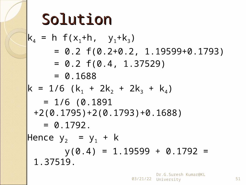
SolutionSolutionk4 = h f(x1+h, y1+k3)
= 0.2 f(0.2+0.2, 1.19599+0.1793) = 0.2 f(0.4, 1.37529) = 0.1688k = 1/6 (k1 + 2k2 + 2k3 + k4)
= 1/6 (0.1891 +2(0.1795)+2(0.1793)+0.1688)
= 0.1792.Hence y2 = y1 + k
y(0.4) = 1.19599 + 0.1792 = 1.37519.
04/19/23 Dr.G.Suresh Kumar@KL University 51
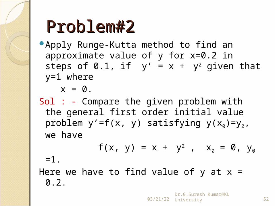
Problem#2Problem#2Apply Runge-Kutta method to find
an approximate value of y for x=0.2 in steps of 0.1, if yʹ = x + y2 given that y=1 where
x = 0.Sol : - Compare the given problem with the
general first order initial value problem yʹ=f(x, y) satisfying y(x0)=y0, we have
f(x, y) = x + y2 , x0 = 0, y0 =1.
Here we have to find value of y at x = 0.2.04/19/23 52Dr.G.Suresh Kumar@KL University

SolutionSolutionTaking step size h = 0.1.Step(1) To find y(0.1) k1 = h f(x0, y0)
= 0.1 f(0, 1) = 0.1 (0 + 12) = 0.1 k2 = h f(x0+0.5h, y0+0.5k1)
= 0.1 f(0+0.5(0.1), 1+ 0.5(0.1)) = 0.2 f(0.05, 1.05) = 0.1152
04/19/23 Dr.G.Suresh Kumar@KL University 53

SolutionSolution
k3 = h f(x0+0.5h, y0+0.5k2)
= 0.1 f(0+0.5(0.1), 1+0.5(0.1152))
= 0.1 f(0.05, 1.0576) = 0.11685 k4 = h f(x0+h, y0+k3)
= 0.1 f(0+0.1, 1+0.11685) = 0.1 f(0.1, 1.11685) = 0.13473
04/19/23 Dr.G.Suresh Kumar@KL University 54

SolutionSolutionk = 1/6 (k1 + 2k2 + 2k3 + k4)
= 1/6 (0.1 +2(0.1152)+2(0.11685)+0.13473)
= 0.11647 ≈ 0.1165.Hence y1 = y0 + k
y(0.1) = 1 + 0.1165 = 1.1165.Step(2) To find y(0.2) k1 = h f(x1, y1)
= 0.1 f(0.1, 1.1165) = 0.1347
04/19/23 Dr.G.Suresh Kumar@KL University 55

solutionsolutionk2 = h f(x1+0.5h, y1+0.5k1)
= 0.1 f(0.1+0.5(0.1), 1.1165+ 0.5(0.1347)) = 0.2 f(0.15, 1.1838) = 0.1551k3 = h f(x1+0.5h, y1+0.5k2)
= 0.1 f(0.1+0.5(0.1), 1.1165+0.5(0.1551)) = 0.1 f(0.15, 1.194) = 0.1575
04/19/23 Dr.G.Suresh Kumar@KL University 56

SolutionSolutionk4 = h f(x1+h, y1+k3)
= 0.1 f(0.1+0.1, 1.1165+0.1576) = 0.1 f(0.2, 1.2741) = 0.1823k = 1/6 (k1 + 2k2 + 2k3 + k4)
= 1/6 (0.1347 +2(0.1551)+2(0.1576)+0.1823)
= 0.1571.Hence y2 = y1 + k
y(0.2) = 1.1165 + 0.1571 = 1.2736.04/19/23 Dr.G.Suresh Kumar@KL University 57