A

PROJECT

REPORT

On

Numerical solutions of ordinary

differential equation using runge kutta method

Submitted by: RENUKA BOKOLIA Research Scholar

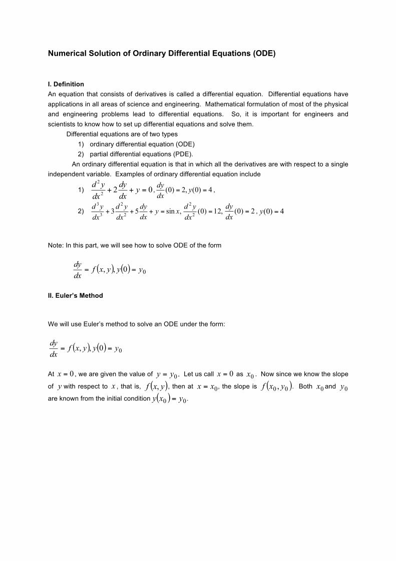
Numerical Solution of Ordinary Differential Equations (ODE) I. Definition An equation that consists of derivatives is called a differential equation. Differential equations have applications in all areas of science and engineering. Mathematical formulation of most of the physical and engineering problems lead to differential equations. So, it is important for engineers and scientists to know how to set up differential equations and solve them. Differential equations are of two types

1) ordinary differential equation (ODE) 2) partial differential equations (PDE).

An ordinary differential equation is that in which all the derivatives are with respect to a single independent variable. Examples of ordinary differential equation include

1) 022

2

=++ ydxdy

dxyd

, 4)0(,2)0( == ydxdy

,

2) ,sin53 2

2

3

3

xydxdy

dxyd

dxyd

=+++ ,12)0(22

=dxyd 2)0( =

dxdy

, 4)0( =y

Note: In this part, we will see how to solve ODE of the form

( ) ( ) 00,, yyyxfdxdy

==

II. Euler’s Method We will use Euler’s method to solve an ODE under the form:

( ) ( ) 00,, yyyxfdxdy

==

At 0=x , we are given the value of .0yy = Let us call 0=x as 0x . Now since we know the slope

of y with respect to x , that is, ( )yxf , , then at 0xx = , the slope is ( )00 , yxf . Both 0x and 0y

are known from the initial condition ( ) 00 yxy = .

Figure 1.Graphical interpretation of the first step of Euler’s method.

So the slope at x=x0as shown in the figure above

Slope 01

01xxyy

−

−=

( )00 , yxf=

Thus

( ) ( )010001 , xxyxfyy −+=

If we consider 01 xx − as a step size h , we get

( ) hyxfyy 0001 ,+= .

We are able now to use the value of 1y (an approximate value of y at 1xx = ) to calculate 2y , which

is the predicted value at 2x ,

( ) hyxfyy 1112 ,+=

hxx += 12

Based on the above equations, if we now know the value of iyy = at ix , then

( ) hyxfyy iiii ,1 +=+

This formula is known as the Euler’s method and is illustrated graphically in Figure 2. In some books, it is also called the Euler-Cauchy method.

Φ

Step size, h

x

y

x0,y0

True value

y1, Predicted value

Figure 2. General graphical interpretation of Euler’s method.

It can be seen that Euler’s method has large errors. This can be illustrated using Taylor series.

( ) ( ) ( ) ...!31

!21 3

1,

3

32

1,

2

2

1,

1 +−+−+−+= ++++ iiyx

iiyx

iiyx

ii xxdxydxx

dxydxx

dxdyyy

iiiiii ( ) ( ) ...),(''!31),('

!21),( 3

12

11 +−+−++= +++ iiiiiiiiiiii xxyxfxxyxfyxfyy

As you can see the first two terms of the Taylor series ( )hyxfyy iiii ,1 +=+ are the Euler’s method.

The true error in the approximation is given by

( ) ( )

...!3,

!2, 32 +

ʹ′ʹ′+

ʹ′= h

yxfh

yxfE iiiit

The true error hence is approximately proportional to the square of the step size, that is, as the step size is halved, the true error gets approximately quartered. However from Table 1, we see that as the step size gets halved, the true error only gets approximately halved. This is because the true error being proportioned to the square of the step size is the local truncation error, that is, error from one point to the next. The global truncation error is however proportional only to the step size as the error keeps propagating from one point to another. II. Runge-Kutta 2nd order

Φ

Step size h

True Value

yi+1, Predicted value

yi

x

y

xi xi+1

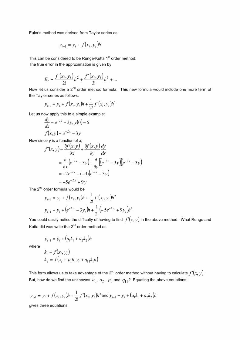
Euler’s method was derived from Taylor series as: ( )hyxfyy iiii ,1 +=+

This can be considered to be Runge-Kutta 1st order method. The true error in the approximation is given by

( ) ( )

...!3,

!2, 32 +

ʹ′ʹ′+

ʹ′= h

yxfh

yxfE iiiit

Now let us consider a 2nd order method formula. This new formula would include one more term of the Taylor series as follows:

( ) ( ) 21 ,

!21, hyxfhyxfyy iiiiii ʹ′++=+

Let us now apply this to a simple example:

( ) 50,32 =−= − yyedxdy x

( ) yeyxf x 3, 2 −= −

Now since y is a function of x,

( ) ( ) ( )dxdy

yyxf

xyxfyxf

∂

∂+

∂

∂=ʹ′

,,,

( ) ( )[ ]( )yeyey

yex

xxx 333 222 −−∂

∂+−

∂

∂= −−−

( )yee xx 3)3(2 22 −−+−= −−

ye x 95 2 +−= −

The 2nd order formula would be

( ) ( ) 21 ,

!21, hyxfhyxfyy iiiiii ʹ′++=+

( ) ( ) 2221 95

!213 hyehyeyy i

xi

xii

ii +−+−+= −−+

You could easily notice the difficulty of having to find ( )yxf ,ʹ′ in the above method. What Runge and

Kutta did was write the 2nd order method as ( )hkakayy ii 22111 ++=+

where ( )ii yxfk ,1 =

( )hkqyhpxfk ii 11112 , ++=

This form allows us to take advantage of the 2nd order method without having to calculate ( )yxf ,ʹ′ .

But, how do we find the unknowns 1a , 2a , 1p and 11q ? Equating the above equations:

( ) ( ) 21 ,

!21, hyxfhyxfyy iiiiii ʹ′++=+ and ( )hkakayy ii 22111 ++=+

gives three equations.

121 =+ aa

21

12 =pa

21

112 =qa

Since we have 3 equations and 4 unknowns, we can assume the value of one of the unknowns. The other three will then be determined from the three equations. Generally the value of 2a is chosen to

evaluate the other three constants. The three values generally used for 2a are21

, 1 and32

, and are

known as Heun’s Method, Midpoint method and Ralston’s method, respectively. II.1. Heun’s method

Here we choose21

2 =a , giving

21

1 =a

11 =p

111 =q

resulting in

hkkyy ii ⎟⎠

⎞⎜⎝

⎛ ++=+ 211 21

21

where ( )ii yxfk ,1 =

( )hkyhxfk ii 12 , ++=

This method is graphically explained in Figure 6.

x

y

xi xi+1

yi+1, predicted

yi

( )ii yxfSlope ,=

( )hkyhxfSlope ii 1, ++=

( ) ( )[ ]iiii yxfhkyhxfSlopeAverage ,,21 1 +++=

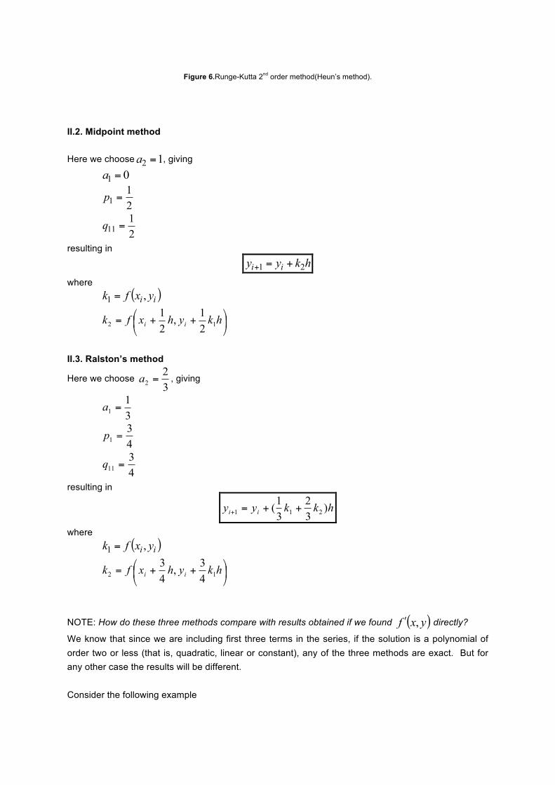
Figure 6.Runge-Kutta 2nd order method(Heun’s method).

II.2. Midpoint method Here we choose 12 =a , giving

01 =a

21

1 =p

21

11 =q

resulting in

hkyy ii 21 +=+

where ( )ii yxfk ,1 =

⎟⎠

⎞⎜⎝

⎛ ++= hkyhxfk ii 12 21,

21

II.3. Ralston’s method

Here we choose 32

2 =a , giving

31

1 =a

43

1 =p

43

11 =q

resulting in

hkkyy ii )32

31( 211 ++=+

where ( )ii yxfk ,1 =

⎟⎠

⎞⎜⎝

⎛ ++= hkyhxfk ii 12 43,

43

NOTE: How do these three methods compare with results obtained if we found ( )yxf ,ʹ′ directly?

We know that since we are including first three terms in the series, if the solution is a polynomial of order two or less (that is, quadratic, linear or constant), any of the three methods are exact. But for any other case the results will be different. Consider the following example

( ) 50,32 =−= − yyedxdy x

If we directly find the ( )yxf ,ʹ′ , the first three terms of Taylor series gives

( ) ( ) 21 ,!21, hyxfhyxfyy iiiiii ʹ′++=+

where

( ) yeyxf x 3, 2 −= −

( ) yeyxf x 95, 2 +−=ʹ′ −

For a step size of 2.0=h , using Heun’s method, we find ( ) 0930.16.0 =y

The exact solution

( ) xx eexy 32 4 −− +=

gives

( ) ( ) ( )6.036.02 46.0 −− += eey

96239.0= Then the absolute relative true error is

10096239.0

0930.196239.0×

−=∈t

%571.13= For the same problem, the results from the Euler and the three Runge-Kuttamethod are given below

Comparison of Euler’s and Runge-Kutta 2nd order methods

y(0.6) Exact Euler Direct 2nd Heun Midpoint Ralston

Value 0.96239 0.4955 1.0930 1.1012 1.0974 1.0994

t∈ % 48.514 13.571 14.423 14.029 14.236

III. Runge-Kutta 4th order Runge-Kutta 4th order method is based on the following

( )hkakakakayy ii 443322111 ++++=+

where knowing the value of iyy = at ix , we can find the value of y=yi+1 at 1+ix , and

ii xxh −= +1

The above equation is equated to the first five terms of Taylor series

( ) ( ) ( )

( )41,4

4

3

1,3

32

1,2

2

1,1

!41

!31

!21

iiyx

iiyxiiyxiiyxii

xxdxyd

xxdxydxx

dxydxx

dxdyyy

ii

iiiiii

−+

−+−+−+=

+

++++

Knowing that ( )yxfdxdy ,= and hxx ii =−+1

( ) ( ) ( ) ( ) 4'''3''2'1 ,

!41,

!31,

!21, hyxfhyxfhyxfhyxfyy iiiiiiiiii ++++=+

Based on equating the above equations, one of the popular solutions used is

( )hkkkkyy ii 43211 2261

++++=+

( )ii yxfk ,1 = This is the slope at xi.

⎟⎠

⎞⎜⎝

⎛ ++= hkyhxfk ii 12 21,

21 This is an estimate of the slope at the midpoint

of the interval [xi,xi+1] using the Euler method to predict the y approximation there.

⎟⎠

⎞⎜⎝

⎛ ++= hkyhxfk ii 23 21,

21 This is an Improved Euler approximation for the slope at

the midpoint. ( )hkyhxfk ii 34 , ++= This is the Euler method slope at xi+1, using the Improved Euler slopek3at the midpoint to step to xi+1. Errors There are two main sources of the total error in numerical approximations: 1. The global truncation error arises from the cumulative effect of two causes: At each step we use an approximate formula to determine yn+1 (leading to a local truncation error). The input data at each step are only approximately correct since in general (tn) yn. 2. Round-off error, also cumulative, arises from using only a finite number of digits.

It can be shown that the global truncation error for the Euler method is proportional to h, for the Improved Euler method is proportional to h2, and for the RungeKutta method is proportional to h4.