Numerical Solution of Interval Nonlinear

System of Equations

A Thesis

submitted in partial fulfilment of the

requirements for the award of the degree of

INTEGRATED MASTER OF SCIENCE

IN

MATHEMATICS

By

Sandeep Nayak

Under the supervision of

Prof. S. Chakraverty

DEPARTMENT OF MATHEMATICS

NATIONAL INSTITUTE OF TECHNOLOGY ROURKELA 769008

ODISHA, INDIA

MAY 2015

ii

NATIONAL INSTITUTE OF TECHNOLOGY

ROURKELA 769008

DECLARATION

I hereby certify that the work which is being presented in the thesis entitled “Numerical

Solution of Interval Nonlinear System of Equations” in partial fulfilment of the requirement

for the award of the degree of Master of Science, submitted in the Department of Mathematics,

National Institute of Technology Rourkela is an authentic record of my own work carried out

under the supervision of Prof. S. Chakraverty.

The matter embodied in this thesis has not been submitted in other institution or university for

the award of any other degree or diploma.

(SANDEEP NAYAK)

This is to certify that the above statement made by the candidate is correct to the best of my

knowledge.

PROF. S. CHAKRAVERTY

Professor, Department of Mathematics

National Institute of Technology

Rourkela 769008

Odisha, India

iii

ACKNOWLEDGEMENT

I would like to warmly acknowledge and convey my deep regards to my project supervisor Dr.

S. Chakraverty, Professor, Department of Mathematics, National Institute of Technology,

Rourkela. I thank him for his patience, keen guidance, constant encouragement and prudent

suggestions during the project, without which this work never come to fruition. Indeed, the

experience of working under him was one of that I will cherish forever.

I am very much grateful to Prof. S. K. Sarangi, Director, National Institute of Technology,

Rourkela for providing excellent facilities in the institute for carrying out research.

I would like to thank all the faculty members of Department of Mathematics for their

cooperation and encouragement. I would like to give heartfelt thanks to Dr. Diptiranjan Behera

and Sukanta Nayak for their valuable suggestions throughout my project work.

I would also like to give my sincere thanks to all of my friends, for their constant efforts and

encouragements, which was the tremendous source of inspiration.

Finally all credits goes to my parents, my brothers and my relatives for their continued support.

And to all mighty, who made all things possible.

Sandeep Nayak

Roll No. 410MA5091

iv

ABSTRACT

Nonlinear system of equations has a wide range of applications in both science and engineering.

But usually the variables and parameters may not be found as crisp numbers. So, the nonlinear

system of equations have been considered in interval form. The basic concepts about interval

arithmetic has been discussed. Three methods has been presented to solve interval nonlinear

system of equations followed by some examples. The interval form is converted to crisp system

of equations by the help of vertex method and then the same may be solved by Newton’s

method. The Krawczyk method has been presented to solve these type of problems too. Finally,

a new method has been proposed which is computationally efficient than vertex method.

Accordingly some examples have been solved using all the methods to show the comparison

and reliability of the methods.

v

TABLE OF CONTENTS

DECLARATION……………………………………………………………………………………….ii

ACKNOWLEDGEMENT…..…………………………………………………………………………iii

ABSTRACT……………………………………………………………………………………………iv

1. INTRODUCTION ................................................................................................................. 1

2. PRELIMINARIES ................................................................................................................. 3

3. DEVELOPED METHODS .................................................................................................... 8

3.1 Interval Nonlinear System of Equations ....................................................................................... 8

3.2 Vertex Method ............................................................................................................................ 10

3.3 Krawczyk Method ....................................................................................................................... 11

3.4 Proposed Method………………………………………………………………………….…... 13

4. NUMERICAL EXAMPLES ................................................................................................ 14

4.1 Examples Solved by Vertex method ........................................................................................... 14

4.2 Example solved by Krawczyk Method ....................................................................................... 18

4.3 Examples Solved by Proposed Method ...................................................................................... 21

5. CONCLUSION .................................................................................................................... 23

6. REFERENCES .................................................................................................................... 24

7. LIST OF PUBLICATIONS ................................................................................................. 26

1

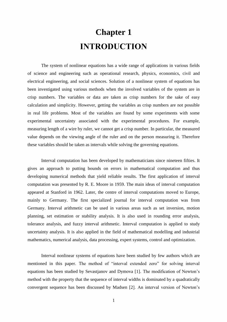
Chapter 1

INTRODUCTION

The system of nonlinear equations has a wide range of applications in various fields

of science and engineering such as operational research, physics, economics, civil and

electrical engineering, and social sciences. Solution of a nonlinear system of equations has

been investigated using various methods when the involved variables of the system are in

crisp numbers. The variables or data are taken as crisp numbers for the sake of easy

calculation and simplicity. However, getting the variables as crisp numbers are not possible

in real life problems. Most of the variables are found by some experiments with some

experimental uncertainty associated with the experimental procedures. For example,

measuring length of a wire by ruler, we cannot get a crisp number. In particular, the measured

value depends on the viewing angle of the ruler and on the person measuring it. Therefore

these variables should be taken as intervals while solving the governing equations.

Interval computation has been developed by mathematicians since nineteen fifties. It

gives an approach to putting bounds on errors in mathematical computation and thus

developing numerical methods that yield reliable results. The first application of interval

computation was presented by R. E. Moore in 1959. The main ideas of interval computation

appeared at Stanford in 1962. Later, the centre of interval computations moved to Europe,

mainly to Germany. The first specialized journal for interval computation was from

Germany. Interval arithmetic can be used in various areas such as set inversion, motion

planning, set estimation or stability analysis. It is also used in rounding error analysis,

tolerance analysis, and fuzzy interval arithmetic. Interval computation is applied to study

uncertainty analysis. It is also applied in the field of mathematical modelling and industrial

mathematics, numerical analysis, data processing, expert systems, control and optimization.

Interval nonlinear systems of equations have been studied by few authors which are

mentioned in this paper. The method of “interval extended zero” for solving interval

equations has been studied by Sevastjanov and Dymova [1]. The modification of Newton’s

method with the property that the sequence of interval widths is dominated by a quadratically

convergent sequence has been discussed by Madsen [2]. An interval version of Newton’s

2

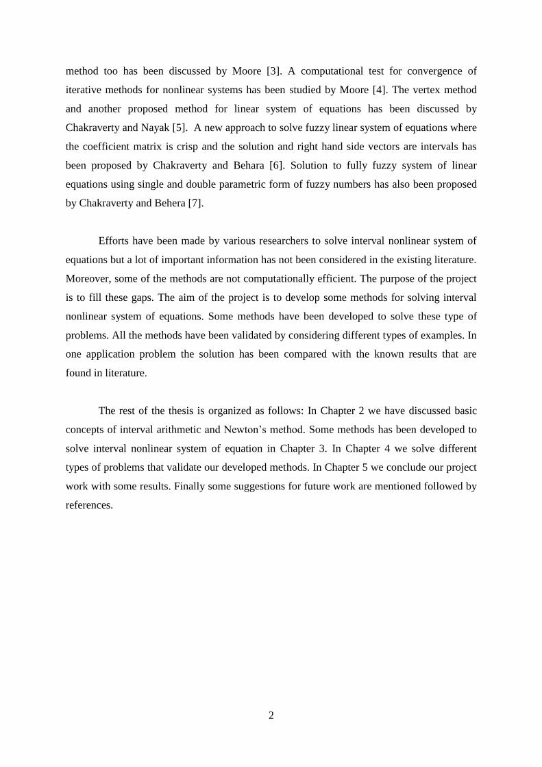
method too has been discussed by Moore [3]. A computational test for convergence of

iterative methods for nonlinear systems has been studied by Moore [4]. The vertex method

and another proposed method for linear system of equations has been discussed by

Chakraverty and Nayak [5]. A new approach to solve fuzzy linear system of equations where

the coefficient matrix is crisp and the solution and right hand side vectors are intervals has

been proposed by Chakraverty and Behara [6]. Solution to fully fuzzy system of linear

equations using single and double parametric form of fuzzy numbers has also been proposed

by Chakraverty and Behera [7].

Efforts have been made by various researchers to solve interval nonlinear system of

equations but a lot of important information has not been considered in the existing literature.

Moreover, some of the methods are not computationally efficient. The purpose of the project

is to fill these gaps. The aim of the project is to develop some methods for solving interval

nonlinear system of equations. Some methods have been developed to solve these type of

problems. All the methods have been validated by considering different types of examples. In

one application problem the solution has been compared with the known results that are

found in literature.

The rest of the thesis is organized as follows: In Chapter 2 we have discussed basic

concepts of interval arithmetic and Newton’s method. Some methods has been developed to

solve interval nonlinear system of equation in Chapter 3. In Chapter 4 we solve different

types of problems that validate our developed methods. In Chapter 5 we conclude our project

work with some results. Finally some suggestions for future work are mentioned followed by

references.

3

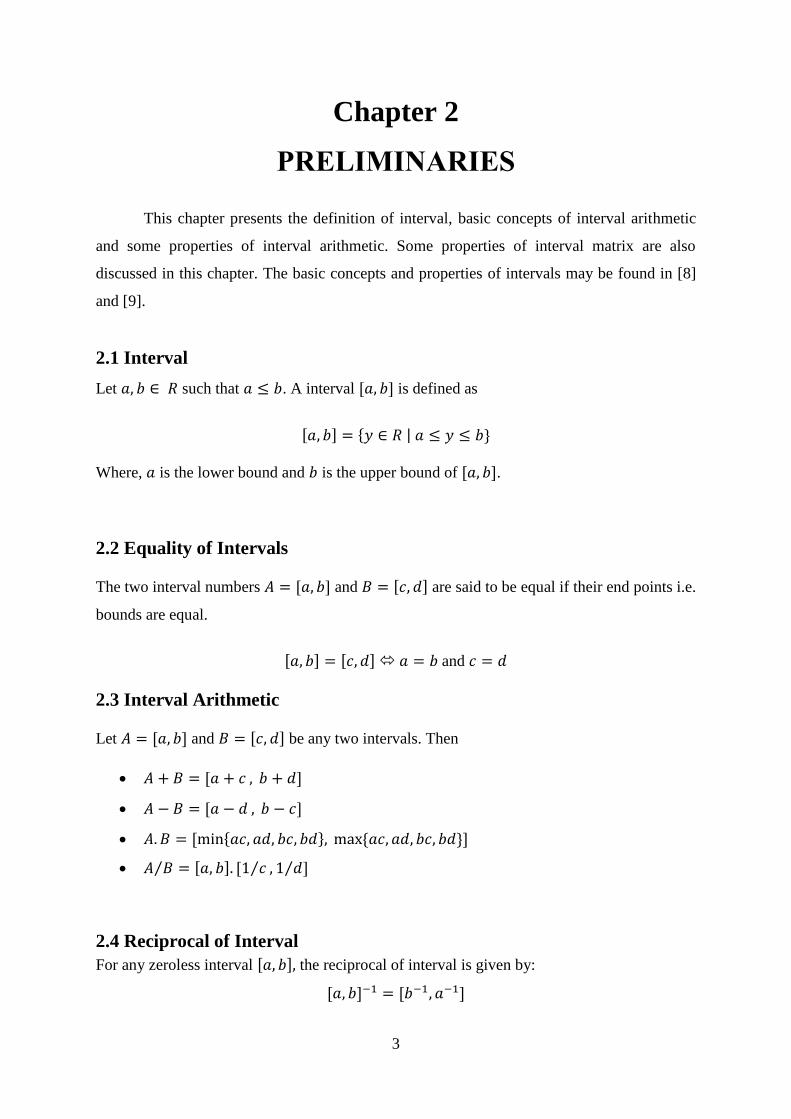
Chapter 2

PRELIMINARIES

This chapter presents the definition of interval, basic concepts of interval arithmetic

and some properties of interval arithmetic. Some properties of interval matrix are also

discussed in this chapter. The basic concepts and properties of intervals may be found in [8]

and [9].

2.1 Interval

Let 𝑎, 𝑏 ∈ 𝑅 such that 𝑎 ≤ 𝑏. A interval [𝑎, 𝑏] is defined as

[𝑎, 𝑏] = {𝑦 ∈ 𝑅 | 𝑎 ≤ 𝑦 ≤ 𝑏}

Where, 𝑎 is the lower bound and 𝑏 is the upper bound of [𝑎, 𝑏].

2.2 Equality of Intervals

The two interval numbers 𝐴 = [𝑎, 𝑏] and 𝐵 = [𝑐, 𝑑] are said to be equal if their end points i.e.

bounds are equal.

[𝑎, 𝑏] = [𝑐, 𝑑] 𝑎 = 𝑏 and 𝑐 = 𝑑

2.3 Interval Arithmetic

Let 𝐴 = [𝑎, 𝑏] and 𝐵 = [𝑐, 𝑑] be any two intervals. Then

𝐴 + 𝐵 = [𝑎 + 𝑐 , 𝑏 + 𝑑]

𝐴 − 𝐵 = [𝑎 − 𝑑 , 𝑏 − 𝑐]

𝐴. 𝐵 = [min{𝑎𝑐, 𝑎𝑑, 𝑏𝑐, 𝑏𝑑}, max {𝑎𝑐, 𝑎𝑑, 𝑏𝑐, 𝑏𝑑}]

𝐴 𝐵 = [𝑎, 𝑏]. [1 𝑐⁄ , 1 𝑑⁄ ]⁄

2.4 Reciprocal of Interval

For any zeroless interval [𝑎, 𝑏], the reciprocal of interval is given by:

[𝑎, 𝑏]−1 = [𝑏−1, 𝑎−1]

4

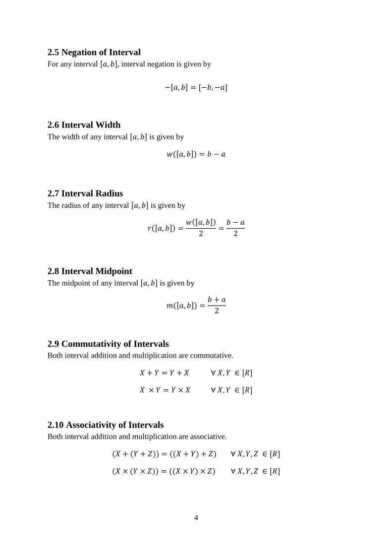
2.5 Negation of Interval

For any interval [𝑎, 𝑏], interval negation is given by

−[𝑎, 𝑏] = [−𝑏,−𝑎]

2.6 Interval Width

The width of any interval [𝑎, 𝑏] is given by

𝑤([𝑎, 𝑏]) = 𝑏 − 𝑎

2.7 Interval Radius

The radius of any interval [𝑎, 𝑏] is given by

𝑟([𝑎, 𝑏]) =𝑤([𝑎, 𝑏])

2=

𝑏 − 𝑎

2

2.8 Interval Midpoint

The midpoint of any interval [𝑎, 𝑏] is given by

𝑚([𝑎, 𝑏]) =𝑏 + 𝑎

2

2.9 Commutativity of Intervals

Both interval addition and multiplication are commutative.

𝑋 + 𝑌 = 𝑌 + 𝑋 ∀ 𝑋, 𝑌 ∈ [𝑅]

𝑋 × 𝑌 = 𝑌 × 𝑋 ∀ 𝑋, 𝑌 ∈ [𝑅]

2.10 Associativity of Intervals

Both interval addition and multiplication are associative.

(𝑋 + (𝑌 + 𝑍)) = ((𝑋 + 𝑌) + 𝑍) ∀ 𝑋, 𝑌, 𝑍 ∈ [𝑅]

(𝑋 × (𝑌 × 𝑍)) = ((𝑋 × 𝑌) × 𝑍) ∀ 𝑋, 𝑌, 𝑍 ∈ [𝑅]

5

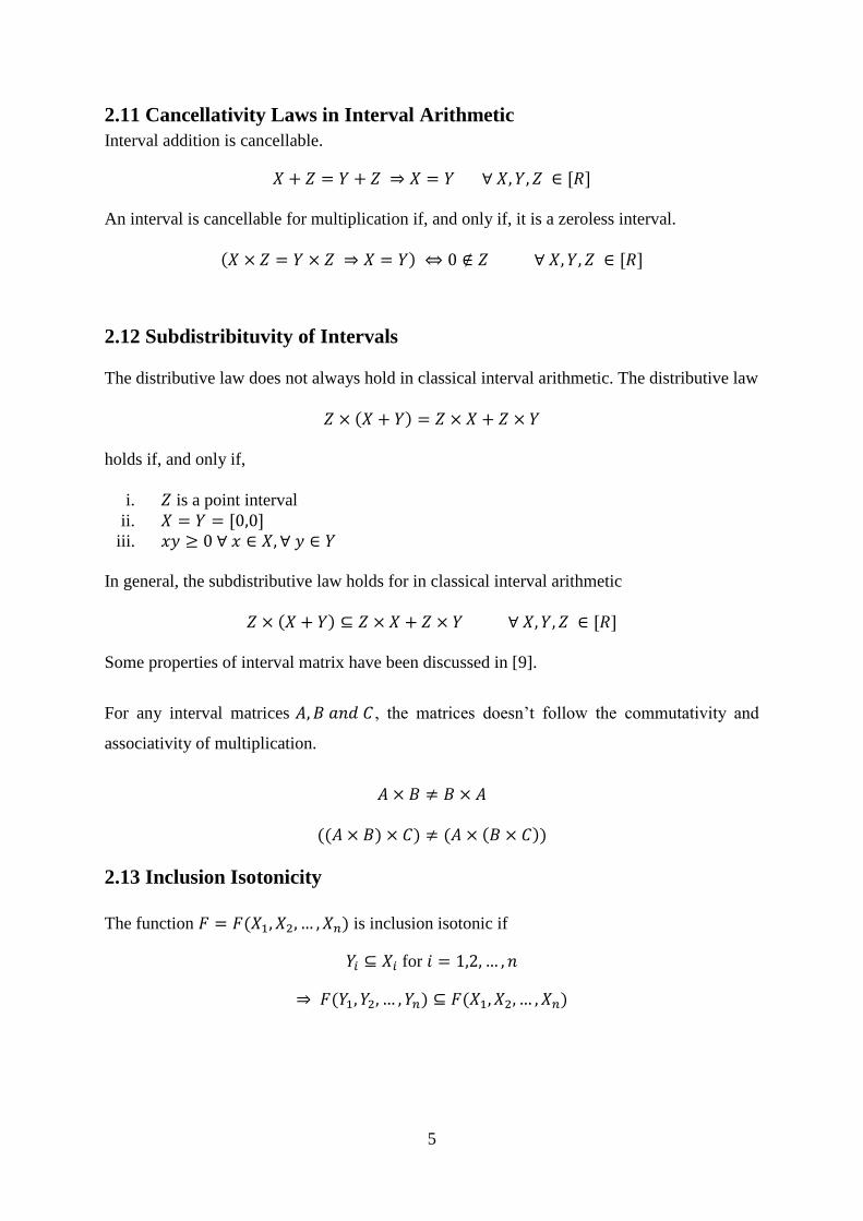
2.11 Cancellativity Laws in Interval Arithmetic

Interval addition is cancellable.

𝑋 + 𝑍 = 𝑌 + 𝑍 ⇒ 𝑋 = 𝑌 ∀ 𝑋, 𝑌, 𝑍 ∈ [𝑅]

An interval is cancellable for multiplication if, and only if, it is a zeroless interval.

(𝑋 × 𝑍 = 𝑌 × 𝑍 ⇒ 𝑋 = 𝑌) ⇔ 0 ∉ 𝑍 ∀ 𝑋, 𝑌, 𝑍 ∈ [𝑅]

2.12 Subdistribituvity of Intervals

The distributive law does not always hold in classical interval arithmetic. The distributive law

𝑍 × (𝑋 + 𝑌) = 𝑍 × 𝑋 + 𝑍 × 𝑌

holds if, and only if,

i. 𝑍 is a point interval

ii. 𝑋 = 𝑌 = [0,0] iii. 𝑥𝑦 ≥ 0 ∀ 𝑥 ∈ 𝑋, ∀ 𝑦 ∈ 𝑌

In general, the subdistributive law holds for in classical interval arithmetic

𝑍 × (𝑋 + 𝑌) ⊆ 𝑍 × 𝑋 + 𝑍 × 𝑌 ∀ 𝑋, 𝑌, 𝑍 ∈ [𝑅]

Some properties of interval matrix have been discussed in [9].

For any interval matrices 𝐴, 𝐵 𝑎𝑛𝑑 𝐶 , the matrices doesn’t follow the commutativity and

associativity of multiplication.

𝐴 × 𝐵 ≠ 𝐵 × 𝐴

((𝐴 × 𝐵) × 𝐶) ≠ (𝐴 × (𝐵 × 𝐶))

2.13 Inclusion Isotonicity

The function 𝐹 = 𝐹(𝑋1, 𝑋2, … , 𝑋𝑛) is inclusion isotonic if

𝑌𝑖 ⊆ 𝑋𝑖 for 𝑖 = 1,2, … , 𝑛

⇒ 𝐹(𝑌1, 𝑌2, … , 𝑌𝑛) ⊆ 𝐹(𝑋1, 𝑋2, … , 𝑋𝑛)

6

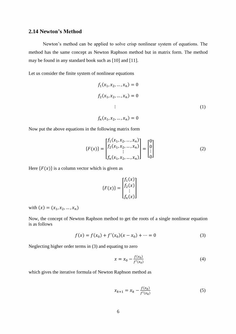
2.14 Newton’s Method

Newton’s method can be applied to solve crisp nonlinear system of equations. The

method has the same concept as Newton Raphson method but in matrix form. The method

may be found in any standard book such as [10] and [11].

Let us consider the finite system of nonlinear equations

𝑓1(𝑥1, 𝑥2, … , 𝑥𝑛) = 0

𝑓2(𝑥1, 𝑥2, … , 𝑥𝑛) = 0

⋮ (1)

𝑓𝑛(𝑥1, 𝑥2, … , 𝑥𝑛) = 0

Now put the above equations in the following matrix form

{𝐹(𝑥)} = [

𝑓1(𝑥1, 𝑥2, … , 𝑥𝑛)

𝑓2(𝑥1, 𝑥2, … , 𝑥𝑛)⋮

𝑓𝑛(𝑥1, 𝑥2, … , 𝑥𝑛)

] = [

00⋮0

] (2)

Here {𝐹(𝑥)} is a column vector which is given as

{𝐹(𝑥)} = [

𝑓1(𝑥)

𝑓2(𝑥)⋮

𝑓𝑛(𝑥)

]

with (𝑥) = (𝑥1, 𝑥2, … , 𝑥𝑛)

Now, the concept of Newton Raphson method to get the roots of a single nonlinear equation

is as follows

𝑓(𝑥) = 𝑓(𝑥0) + 𝑓′(𝑥0)(𝑥 − 𝑥0) + ⋯ = 0 (3)

Neglecting higher order terms in (3) and equating to zero

𝑥 = 𝑥0 −𝑓(𝑥0)

𝑓′(𝑥0) (4)

which gives the iterative formula of Newton Raphson method as

𝑥𝑘+1 = 𝑥𝑘 −𝑓(𝑥𝑘)

𝑓′(𝑥𝑘) (5)

7

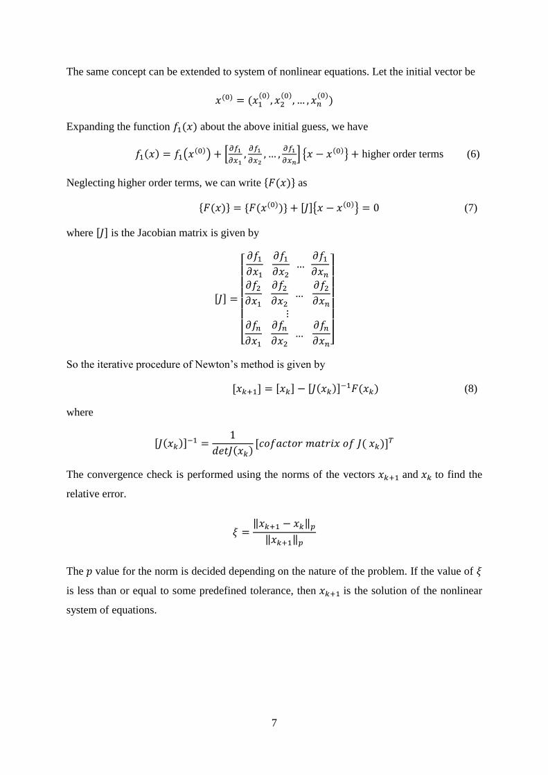
The same concept can be extended to system of nonlinear equations. Let the initial vector be

𝑥(0) = (𝑥1(0)

, 𝑥2(0)

, … , 𝑥𝑛(0)

)

Expanding the function 𝑓1(𝑥) about the above initial guess, we have

𝑓1(𝑥) = 𝑓1(𝑥(0)) + [

𝜕𝑓1

𝜕𝑥1,𝜕𝑓1

𝜕𝑥2, … ,

𝜕𝑓1

𝜕𝑥𝑛] {𝑥 − 𝑥(0)} + higher order terms (6)

Neglecting higher order terms, we can write {𝐹(𝑥)} as

{𝐹(𝑥)} = {𝐹(𝑥(0))} + [𝐽]{𝑥 − 𝑥(0)} = 0 (7)

where [𝐽] is the Jacobian matrix is given by

[𝐽] =

[ 𝜕𝑓1𝜕𝑥1

𝜕𝑓1𝜕𝑥2

… 𝜕𝑓1𝜕𝑥𝑛

𝜕𝑓2𝜕𝑥1

𝜕𝑓2𝜕𝑥2

… 𝜕𝑓2𝜕𝑥𝑛

⋮𝜕𝑓𝑛𝜕𝑥1

𝜕𝑓𝑛𝜕𝑥2

… 𝜕𝑓𝑛𝜕𝑥𝑛]

So the iterative procedure of Newton’s method is given by

[𝑥𝑘+1] = [𝑥𝑘] − [𝐽(𝑥𝑘)]−1𝐹(𝑥𝑘) (8)

where

[𝐽(𝑥𝑘)]−1 =

1

𝑑𝑒𝑡𝐽(𝑥𝑘)[𝑐𝑜𝑓𝑎𝑐𝑡𝑜𝑟 𝑚𝑎𝑡𝑟𝑖𝑥 𝑜𝑓 𝐽( 𝑥𝑘)]

𝑇

The convergence check is performed using the norms of the vectors 𝑥𝑘+1 and 𝑥𝑘 to find the

relative error.

𝜉 =‖𝑥𝑘+1 − 𝑥𝑘‖𝑝

‖𝑥𝑘+1‖𝑝

The 𝑝 value for the norm is decided depending on the nature of the problem. If the value of 𝜉

is less than or equal to some predefined tolerance, then 𝑥𝑘+1 is the solution of the nonlinear

system of equations.

8

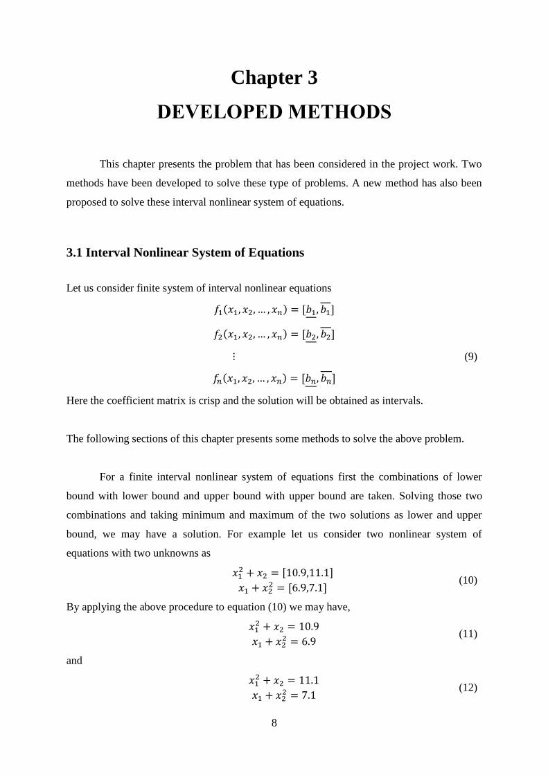
Chapter 3

DEVELOPED METHODS

This chapter presents the problem that has been considered in the project work. Two

methods have been developed to solve these type of problems. A new method has also been

proposed to solve these interval nonlinear system of equations.

3.1 Interval Nonlinear System of Equations

Let us consider finite system of interval nonlinear equations

𝑓1(𝑥1, 𝑥2, … , 𝑥𝑛) = [𝑏1, 𝑏1]

𝑓2(𝑥1, 𝑥2, … , 𝑥𝑛) = [𝑏2, 𝑏2]

⋮ (9)

𝑓𝑛(𝑥1, 𝑥2, … , 𝑥𝑛) = [𝑏𝑛, 𝑏𝑛]

Here the coefficient matrix is crisp and the solution will be obtained as intervals.

The following sections of this chapter presents some methods to solve the above problem.

For a finite interval nonlinear system of equations first the combinations of lower

bound with lower bound and upper bound with upper bound are taken. Solving those two

combinations and taking minimum and maximum of the two solutions as lower and upper

bound, we may have a solution. For example let us consider two nonlinear system of

equations with two unknowns as

𝑥12 + 𝑥2 = [10.9,11.1]

𝑥1 + 𝑥22 = [6.9,7.1]

(10)

By applying the above procedure to equation (10) we may have,

𝑥1

2 + 𝑥2 = 10.9

𝑥1 + 𝑥22 = 6.9

(11)

and

𝑥1

2 + 𝑥2 = 11.1

𝑥1 + 𝑥22 = 7.1

(12)

9

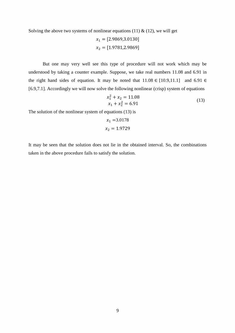
Solving the above two systems of nonlinear equations (11) & (12), we will get

𝑥1 = [2.9869,3.0130]

𝑥2 = [1.9781,2.9869]

But one may very well see this type of procedure will not work which may be

understood by taking a counter example. Suppose, we take real numbers 11.08 and 6.91 in

the right hand sides of equation. It may be noted that 11.08 ∈ [10.9,11.1] and 6.91 ∈

[6.9,7.1]. Accordingly we will now solve the following nonlinear (crisp) system of equations

𝑥1

2 + 𝑥2 = 11.08

𝑥1 + 𝑥22 = 6.91

(13)

The solution of the nonlinear system of equations (13) is

𝑥1 =3.0178

𝑥2 = 1.9729

It may be seen that the solution does not lie in the obtained interval. So, the combinations

taken in the above procedure fails to satisfy the solution.

10

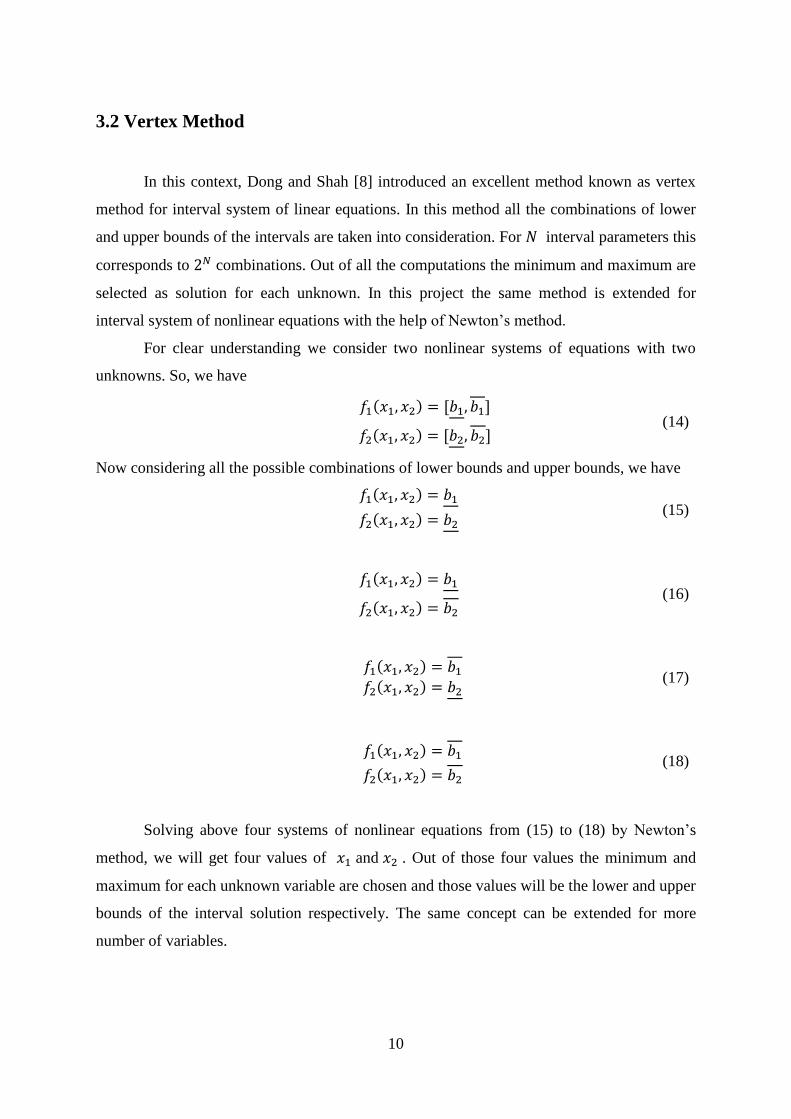
3.2 Vertex Method

In this context, Dong and Shah [8] introduced an excellent method known as vertex

method for interval system of linear equations. In this method all the combinations of lower

and upper bounds of the intervals are taken into consideration. For 𝑁 interval parameters this

corresponds to 2𝑁 combinations. Out of all the computations the minimum and maximum are

selected as solution for each unknown. In this project the same method is extended for

interval system of nonlinear equations with the help of Newton’s method.

For clear understanding we consider two nonlinear systems of equations with two

unknowns. So, we have

𝑓1(𝑥1, 𝑥2) = [𝑏1, 𝑏1]

𝑓2(𝑥1, 𝑥2) = [𝑏2, 𝑏2] (14)

Now considering all the possible combinations of lower bounds and upper bounds, we have

𝑓1(𝑥1, 𝑥2) = 𝑏1

𝑓2(𝑥1, 𝑥2) = 𝑏2 (15)

𝑓1(𝑥1, 𝑥2) = 𝑏1

𝑓2(𝑥1, 𝑥2) = 𝑏2

(16)

𝑓1(𝑥1, 𝑥2) = 𝑏1

𝑓2(𝑥1, 𝑥2) = 𝑏2 (17)

𝑓1(𝑥1, 𝑥2) = 𝑏1

𝑓2(𝑥1, 𝑥2) = 𝑏2

(18)

Solving above four systems of nonlinear equations from (15) to (18) by Newton’s

method, we will get four values of 𝑥1 and 𝑥2 . Out of those four values the minimum and

maximum for each unknown variable are chosen and those values will be the lower and upper

bounds of the interval solution respectively. The same concept can be extended for more

number of variables.

11

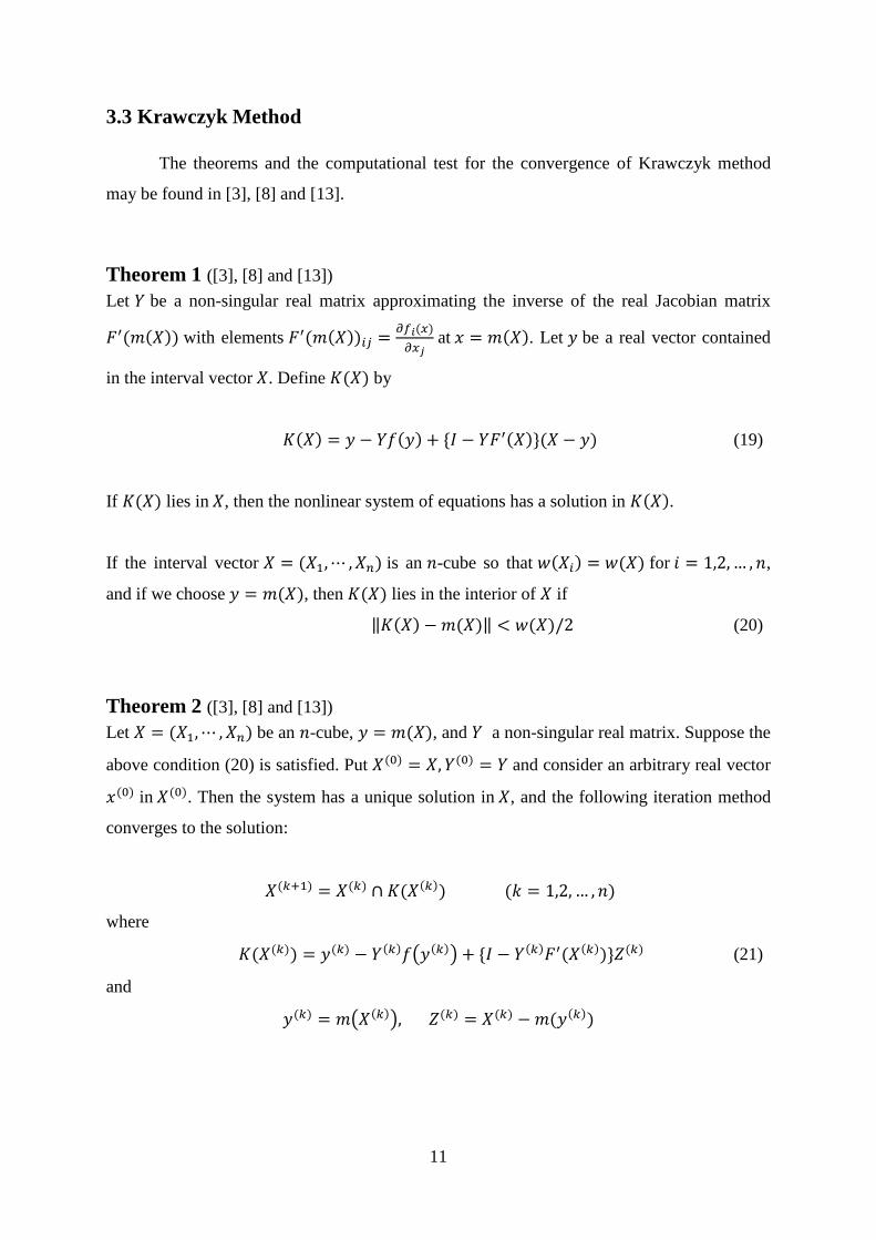
3.3 Krawczyk Method

The theorems and the computational test for the convergence of Krawczyk method

may be found in [3], [8] and [13].

Theorem 1 ([3], [8] and [13])

Let 𝑌 be a non-singular real matrix approximating the inverse of the real Jacobian matrix

𝐹′(𝑚(𝑋)) with elements 𝐹′(𝑚(𝑋))𝑖𝑗 =𝜕𝑓𝑖(𝑥)

𝜕𝑥𝑗 at 𝑥 = 𝑚(𝑋). Let 𝑦 be a real vector contained

in the interval vector 𝑋. Define 𝐾(𝑋) by

𝐾(𝑋) = 𝑦 − 𝑌𝑓(𝑦) + {𝐼 − 𝑌𝐹′(𝑋)}(𝑋 − 𝑦) (19)

If 𝐾(𝑋) lies in 𝑋, then the nonlinear system of equations has a solution in 𝐾(𝑋).

If the interval vector 𝑋 = (𝑋1,⋯ , 𝑋𝑛) is an 𝑛-cube so that 𝑤(𝑋𝑖) = 𝑤(𝑋) for 𝑖 = 1,2, … , 𝑛,

and if we choose 𝑦 = 𝑚(𝑋), then 𝐾(𝑋) lies in the interior of 𝑋 if

‖𝐾(𝑋) − 𝑚(𝑋)‖ < 𝑤(𝑋)/2 (20)

Theorem 2 ([3], [8] and [13])

Let 𝑋 = (𝑋1,⋯ , 𝑋𝑛) be an 𝑛-cube, 𝑦 = 𝑚(𝑋), and 𝑌 a non-singular real matrix. Suppose the

above condition (20) is satisfied. Put 𝑋(0) = 𝑋, 𝑌(0) = 𝑌 and consider an arbitrary real vector

𝑥(0) in 𝑋(0). Then the system has a unique solution in 𝑋, and the following iteration method

converges to the solution:

𝑋(𝑘+1) = 𝑋(𝑘) ∩ 𝐾(𝑋(𝑘)) (𝑘 = 1,2, … , 𝑛)

where

𝐾(𝑋(𝑘)) = 𝑦(𝑘) − 𝑌(𝑘)𝑓(𝑦(𝑘)) + {𝐼 − 𝑌(𝑘)𝐹′(𝑋(𝑘))}𝑍(𝑘) (21)

and

𝑦(𝑘) = 𝑚(𝑋(𝑘)), 𝑍(𝑘) = 𝑋(𝑘) − 𝑚(𝑦(𝑘))

12

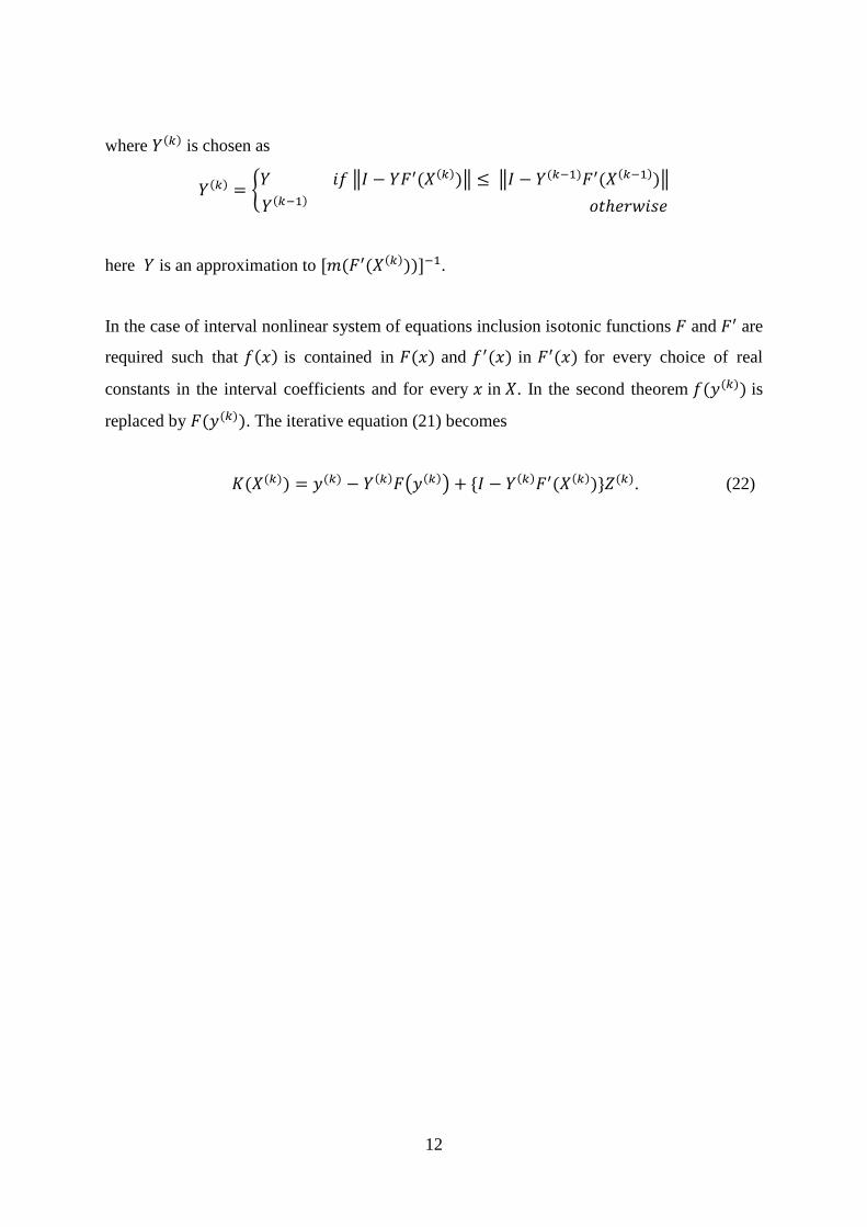
where 𝑌(𝑘) is chosen as

𝑌(𝑘) = {𝑌 𝑖𝑓 ‖𝐼 − 𝑌𝐹′(𝑋(𝑘))‖ ≤ ‖𝐼 − 𝑌(𝑘−1)𝐹′(𝑋(𝑘−1))‖

𝑌(𝑘−1) 𝑜𝑡ℎ𝑒𝑟𝑤𝑖𝑠𝑒

here 𝑌 is an approximation to [𝑚(𝐹′(𝑋(𝑘)))]−1.

In the case of interval nonlinear system of equations inclusion isotonic functions 𝐹 and 𝐹′ are

required such that 𝑓(𝑥) is contained in 𝐹(𝑥) and 𝑓′(𝑥) in 𝐹′(𝑥) for every choice of real

constants in the interval coefficients and for every 𝑥 in 𝑋. In the second theorem 𝑓(𝑦(𝑘)) is

replaced by 𝐹(𝑦(𝑘)). The iterative equation (21) becomes

𝐾(𝑋(𝑘)) = 𝑦(𝑘) − 𝑌(𝑘)𝐹(𝑦(𝑘)) + {𝐼 − 𝑌(𝑘)𝐹′(𝑋(𝑘))}𝑍(𝑘). (22)

13

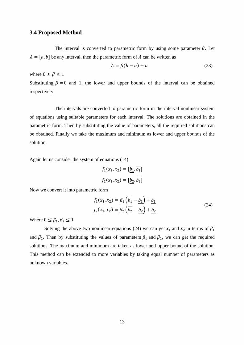
3.4 Proposed Method

The interval is converted to parametric form by using some parameter 𝛽. Let

𝐴 = [𝑎, 𝑏] be any interval, then the parametric form of 𝐴 can be written as

𝐴 = 𝛽(𝑏 − 𝑎) + 𝑎 (23)

where 0 ≤ 𝛽 ≤ 1

Substituting 𝛽 =0 and 1, the lower and upper bounds of the interval can be obtained

respectively.

The intervals are converted to parametric form in the interval nonlinear system

of equations using suitable parameters for each interval. The solutions are obtained in the

parametric form. Then by substituting the value of parameters, all the required solutions can

be obtained. Finally we take the maximum and minimum as lower and upper bounds of the

solution.

Again let us consider the system of equations (14)

𝑓1(𝑥1, 𝑥2) = [𝑏1, 𝑏1]

𝑓2(𝑥1, 𝑥2) = [𝑏2, 𝑏2]

Now we convert it into parametric form

𝑓1(𝑥1, 𝑥2) = 𝛽1 (𝑏1 − 𝑏1) + 𝑏1

𝑓2(𝑥1, 𝑥2) = 𝛽2 (𝑏2 − 𝑏2) + 𝑏2

(24)

Where 0 ≤ 𝛽1, 𝛽2 ≤ 1

Solving the above two nonlinear equations (24) we can get 𝑥1 and 𝑥2 in terms of 𝛽1

and 𝛽2. Then by substituting the values of parameters 𝛽1 and 𝛽2, we can get the required

solutions. The maximum and minimum are taken as lower and upper bound of the solution.

This method can be extended to more variables by taking equal number of parameters as

unknown variables.

14

Chapter 4

NUMERICAL EXAMPLES

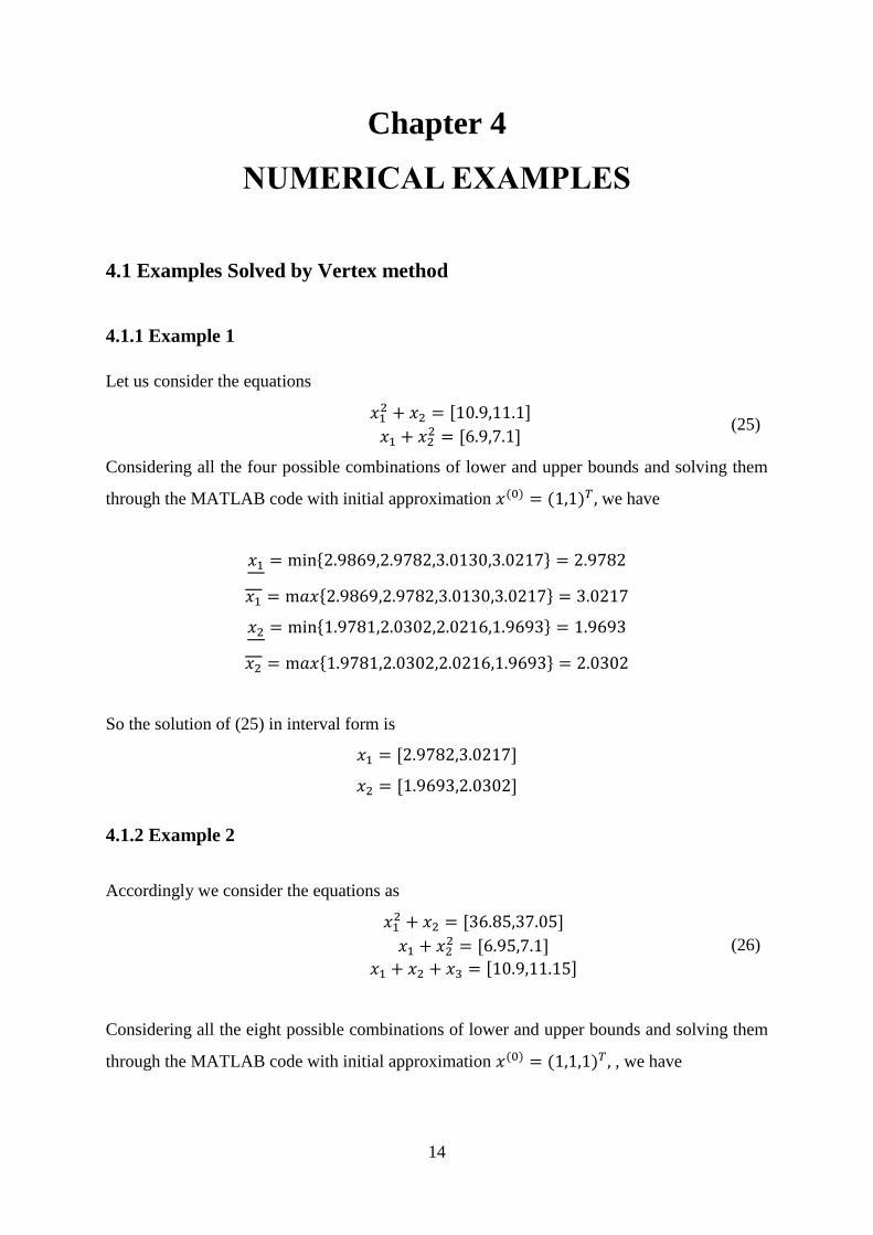
4.1 Examples Solved by Vertex method

4.1.1 Example 1

Let us consider the equations

𝑥12 + 𝑥2 = [10.9,11.1]

𝑥1 + 𝑥22 = [6.9,7.1]

(25)

Considering all the four possible combinations of lower and upper bounds and solving them

through the MATLAB code with initial approximation 𝑥(0) = (1,1)𝑇 , we have

𝑥1 = min{2.9869,2.9782,3.0130,3.0217} = 2.9782

𝑥1 = m𝑎𝑥{2.9869,2.9782,3.0130,3.0217} = 3.0217

𝑥2 = min{1.9781,2.0302,2.0216,1.9693} = 1.9693

𝑥2 = m𝑎𝑥{1.9781,2.0302,2.0216,1.9693} = 2.0302

So the solution of (25) in interval form is

𝑥1 = [2.9782,3.0217]

𝑥2 = [1.9693,2.0302]

4.1.2 Example 2

Accordingly we consider the equations as

𝑥12 + 𝑥2 = [36.85,37.05]

𝑥1 + 𝑥22 = [6.95,7.1]

𝑥1 + 𝑥2 + 𝑥3 = [10.9,11.15]

(26)

Considering all the eight possible combinations of lower and upper bounds and solving them

through the MATLAB code with initial approximation 𝑥(0) = (1,1,1)𝑇 , , we have

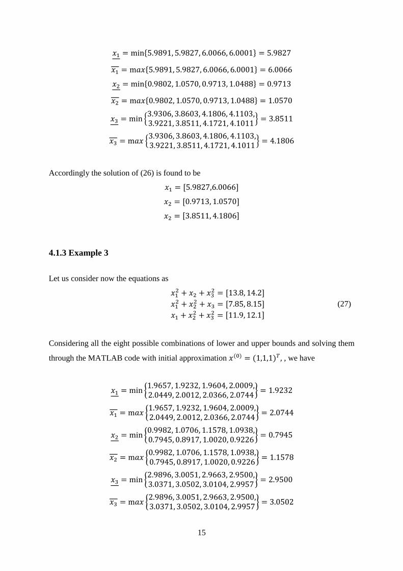
15

𝑥1 = min{5.9891, 5.9827, 6.0066, 6.0001} = 5.9827

𝑥1 = m𝑎𝑥{5.9891, 5.9827, 6.0066, 6.0001} = 6.0066

𝑥2 = min{0.9802, 1.0570, 0.9713, 1.0488} = 0.9713

𝑥2 = m𝑎𝑥{0.9802, 1.0570, 0.9713, 1.0488} = 1.0570

𝑥3 = min {3.9306, 3.8603, 4.1806, 4.1103,3.9221, 3.8511, 4.1721, 4.1011

} = 3.8511

𝑥3 = m𝑎𝑥 {3.9306, 3.8603, 4.1806, 4.1103,3.9221, 3.8511, 4.1721, 4.1011

} = 4.1806

Accordingly the solution of (26) is found to be

𝑥1 = [5.9827,6.0066]

𝑥2 = [0.9713, 1.0570]

𝑥2 = [3.8511, 4.1806]

4.1.3 Example 3

Let us consider now the equations as

𝑥12 + 𝑥2 + 𝑥3

2 = [13.8, 14.2]

𝑥12 + 𝑥2

2 + 𝑥3 = [7.85, 8.15]

𝑥1 + 𝑥22 + 𝑥3

2 = [11.9, 12.1]

(27)

Considering all the eight possible combinations of lower and upper bounds and solving them

through the MATLAB code with initial approximation 𝑥(0) = (1,1,1)𝑇 , , we have

𝑥1 = min {1.9657, 1.9232, 1.9604, 2.0009,2.0449, 2.0012, 2.0366, 2.0744

} = 1.9232

𝑥1 = m𝑎𝑥 {1.9657, 1.9232, 1.9604, 2.0009,2.0449, 2.0012, 2.0366, 2.0744

} = 2.0744

𝑥2 = min {0.9982, 1.0706, 1.1578, 1.0938,0.7945, 0.8917, 1.0020, 0.9226

} = 0.7945

𝑥2 = m𝑎𝑥 {0.9982, 1.0706, 1.1578, 1.0938,0.7945, 0.8917, 1.0020, 0.9226

} = 1.1578

𝑥3 = min {2.9896, 3.0051, 2.9663, 2.9500,3.0371, 3.0502, 3.0104, 2.9957

} = 2.9500

𝑥3 = m𝑎𝑥 {2.9896, 3.0051, 2.9663, 2.9500,3.0371, 3.0502, 3.0104, 2.9957

} = 3.0502

16

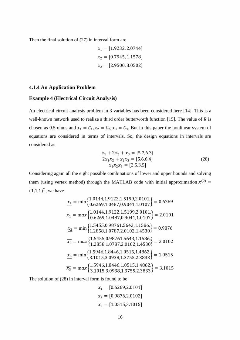
Then the final solution of (27) in interval form are

𝑥1 = [1.9232, 2.0744]

𝑥2 = [0.7945, 1.1578]

𝑥2 = [2.9500, 3.0502]

4.1.4 An Application Problem

Example 4 (Electrical Circuit Analysis)

An electrical circuit analysis problem in 3 variables has been considered here [14]. This is a

well-known network used to realize a third order butterworth function [15]. The value of 𝑅 is

chosen as 0.5 ohms and 𝑥1 = 𝐶1, 𝑥2 = 𝐶2, 𝑥3 = 𝐶3. But in this paper the nonlinear system of

equations are considered in terms of intervals. So, the design equations in intervals are

considered as

𝑥1 + 2𝑥2 + 𝑥3 = [5.7,6.3]

2𝑥1𝑥2 + 𝑥2𝑥3 = [5.6,6.4]

𝑥1𝑥2𝑥3 = [2.5,3.5] (28)

Considering again all the eight possible combinations of lower and upper bounds and solving

them (using vertex method) through the MATLAB code with initial approximation 𝑥(0) =

(1,1,1)𝑇, we have

𝑥1 = min {1.0144,1.9122,1.5199,2.0101,0.6269,1.0487,0.9041,1.0107

} = 0.6269

𝑥1 = m𝑎𝑥 {1.0144,1.9122,1.5199,2.0101,0.6269,1.0487,0.9041,1.0107

} = 2.0101

𝑥2 = min {1.5455,0.98761.5643,1.1586,1.2858,1.0787,2.0102,1.4530

} = 0.9876

𝑥2 = m𝑎𝑥 {1.5455,0.98761.5643,1.1586,1.2858,1.0787,2.0102,1.4530

} = 2.0102

𝑥3 = min {1.5946,1.8446,1.0515,1.4862,3.1015,3.0938,1.3755,2.3833

} = 1.0515

𝑥3 = m𝑎𝑥 {1.5946,1.8446,1.0515,1.4862,3.1015,3.0938,1.3755,2.3833

} = 3.1015

The solution of (28) in interval form is found to be

𝑥1 = [0.6269,2.0101]

𝑥2 = [0.9876,2.0102]

𝑥3 = [1.0515,3.1015]

17

Now with another initial approximation 𝑥(0) = (4,0,1)𝑇, the solution of (28) is found to be

𝑥1 = [1.9122,4.0703]

𝑥2 = [0.6121,1.1586]

𝑥3 = [0.8661,1.8446]

It may be seen that both the operating points of the butterworth function problem [14] lie in

the obtained intervals using vertex method.

18

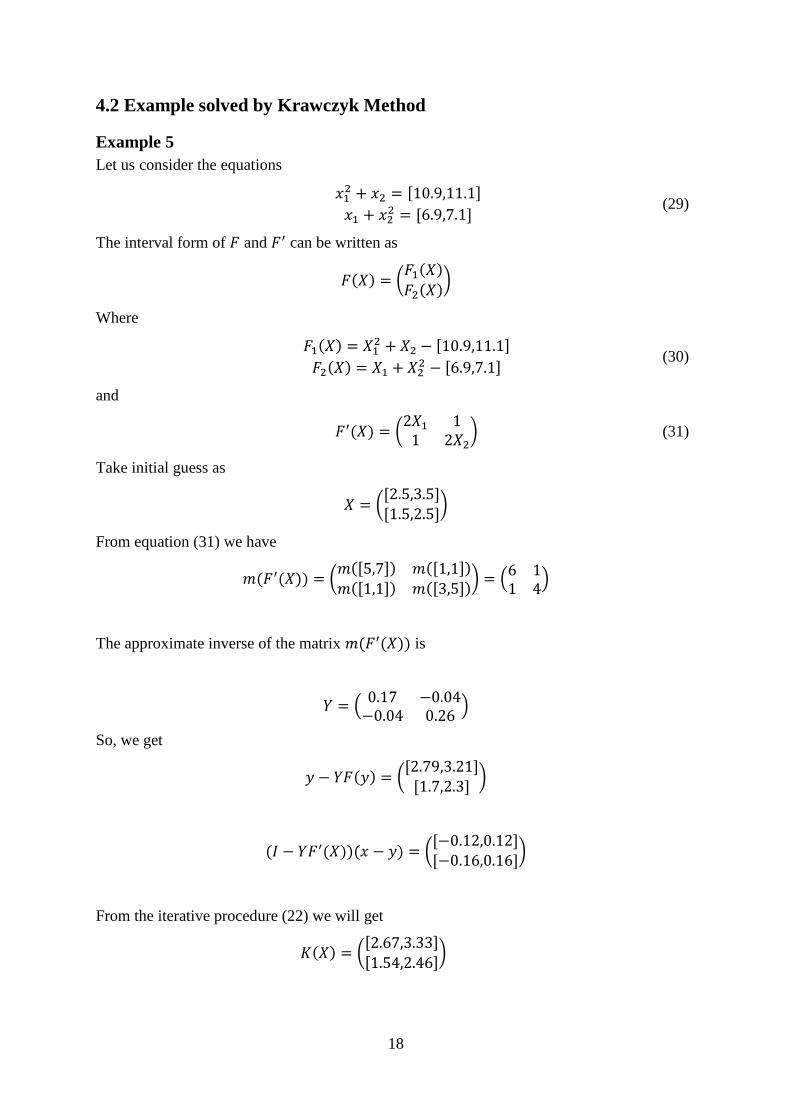
4.2 Example solved by Krawczyk Method

Example 5

Let us consider the equations

𝑥12 + 𝑥2 = [10.9,11.1]

𝑥1 + 𝑥22 = [6.9,7.1]

(29)

The interval form of 𝐹 and 𝐹′ can be written as

𝐹(𝑋) = (𝐹1(𝑋)

𝐹2(𝑋))

Where

𝐹1(𝑋) = 𝑋1

2 + 𝑋2 − [10.9,11.1]

𝐹2(𝑋) = 𝑋1 + 𝑋22 − [6.9,7.1]

(30)

and

𝐹′(𝑋) = (2𝑋1 11 2𝑋2

) (31)

Take initial guess as

𝑋 = ([2.5,3.5][1.5,2.5]

)

From equation (31) we have

𝑚(𝐹′(𝑋)) = (𝑚([5,7]) 𝑚([1,1])

𝑚([1,1]) 𝑚([3,5])) = (

6 11 4

)

The approximate inverse of the matrix 𝑚(𝐹′(𝑋)) is

𝑌 = (0.17 −0.04

−0.04 0.26)

So, we get

𝑦 − 𝑌𝐹(𝑦) = ([2.79,3.21][1.7,2.3]

)

(𝐼 − 𝑌𝐹′(𝑋))(𝑥 − 𝑦) = ([−0.12,0.12][−0.16,0.16]

)

From the iterative procedure (22) we will get

𝐾(𝑋) = ([2.67,3.33]

[1.54,2.46])

19

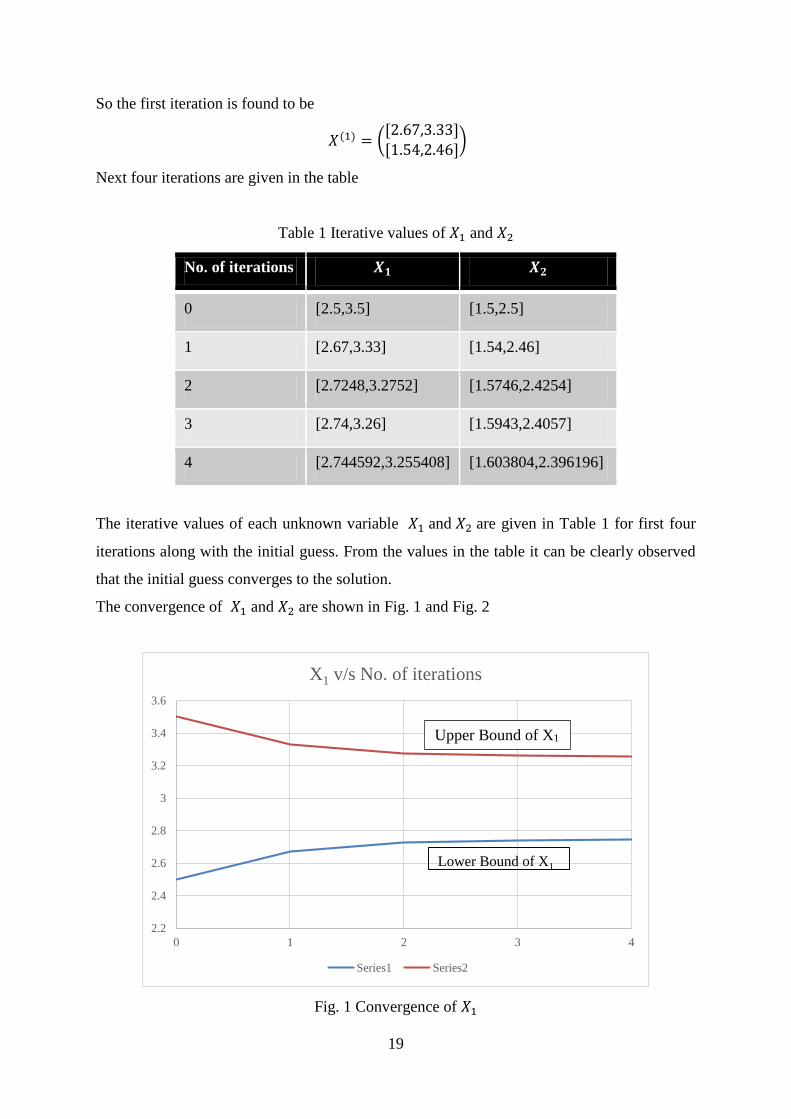
So the first iteration is found to be

𝑋(1) = ([2.67,3.33][1.54,2.46]

)

Next four iterations are given in the table

Table 1 Iterative values of 𝑋1 and 𝑋2

No. of iterations 𝑿𝟏 𝑿𝟐

0 [2.5,3.5] [1.5,2.5]

1 [2.67,3.33] [1.54,2.46]

2 [2.7248,3.2752] [1.5746,2.4254]

3 [2.74,3.26] [1.5943,2.4057]

4 [2.744592,3.255408] [1.603804,2.396196]

The iterative values of each unknown variable 𝑋1 and 𝑋2 are given in Table 1 for first four

iterations along with the initial guess. From the values in the table it can be clearly observed

that the initial guess converges to the solution.

The convergence of 𝑋1 and 𝑋2 are shown in Fig. 1 and Fig. 2

Fig. 1 Convergence of 𝑋1

2.2

2.4

2.6

2.8

3

3.2

3.4

3.6

0 1 2 3 4

X1 v/s No. of iterations

Series1 Series2

Lower Bound of X1

Upper Bound of X1

20

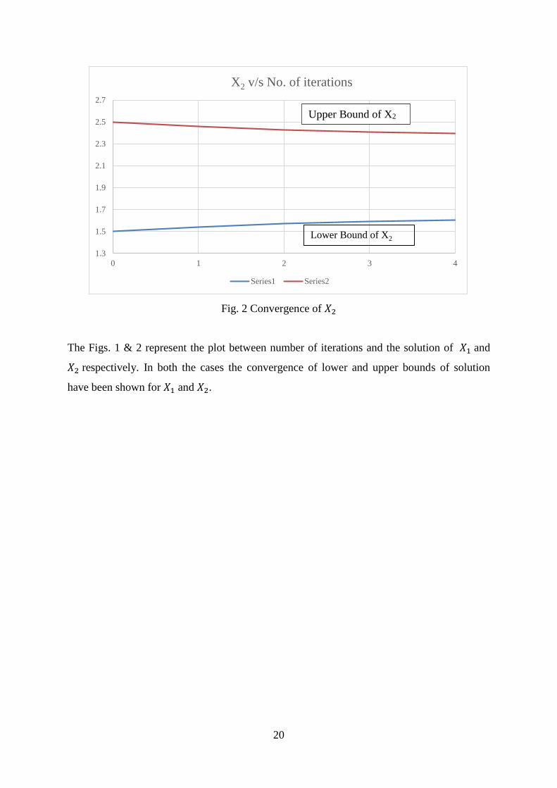
Fig. 2 Convergence of 𝑋2

The Figs. 1 & 2 represent the plot between number of iterations and the solution of 𝑋1 and

𝑋2 respectively. In both the cases the convergence of lower and upper bounds of solution

have been shown for 𝑋1 and 𝑋2.

1.3

1.5

1.7

1.9

2.1

2.3

2.5

2.7

0 1 2 3 4

X2 v/s No. of iterations

Series1 Series2

Lower Bound of X2

Upper Bound of X2

21

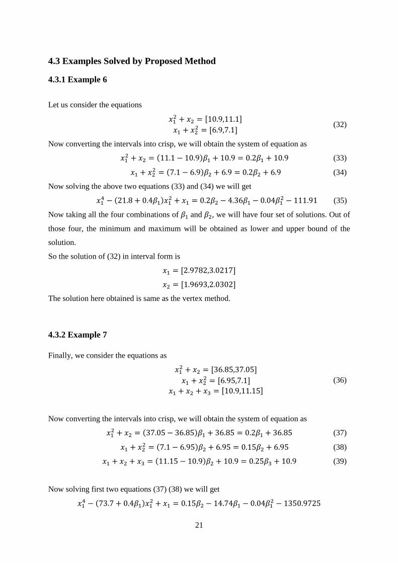
4.3 Examples Solved by Proposed Method

4.3.1 Example 6

Let us consider the equations

𝑥12 + 𝑥2 = [10.9,11.1]

𝑥1 + 𝑥22 = [6.9,7.1]

(32)

Now converting the intervals into crisp, we will obtain the system of equation as

𝑥12 + 𝑥2 = (11.1 − 10.9)𝛽1 + 10.9 = 0.2𝛽1 + 10.9 (33)

𝑥1 + 𝑥22 = (7.1 − 6.9)𝛽2 + 6.9 = 0.2𝛽2 + 6.9 (34)

Now solving the above two equations (33) and (34) we will get

𝑥14 − (21.8 + 0.4𝛽1)𝑥1

2 + 𝑥1 = 0.2𝛽2 − 4.36𝛽1 − 0.04𝛽12 − 111.91 (35)

Now taking all the four combinations of 𝛽1 and 𝛽2, we will have four set of solutions. Out of

those four, the minimum and maximum will be obtained as lower and upper bound of the

solution.

So the solution of (32) in interval form is

𝑥1 = [2.9782,3.0217]

𝑥2 = [1.9693,2.0302]

The solution here obtained is same as the vertex method.

4.3.2 Example 7

Finally, we consider the equations as

𝑥12 + 𝑥2 = [36.85,37.05]

𝑥1 + 𝑥22 = [6.95,7.1]

𝑥1 + 𝑥2 + 𝑥3 = [10.9,11.15]

(36)

Now converting the intervals into crisp, we will obtain the system of equation as

𝑥12 + 𝑥2 = (37.05 − 36.85)𝛽1 + 36.85 = 0.2𝛽1 + 36.85 (37)

𝑥1 + 𝑥22 = (7.1 − 6.95)𝛽2 + 6.95 = 0.15𝛽2 + 6.95 (38)

𝑥1 + 𝑥2 + 𝑥3 = (11.15 − 10.9)𝛽2 + 10.9 = 0.25𝛽3 + 10.9 (39)

Now solving first two equations (37) (38) we will get

𝑥14 − (73.7 + 0.4𝛽1)𝑥1

2 + 𝑥1 = 0.15𝛽2 − 14.74𝛽1 − 0.04𝛽12 − 1350.9725

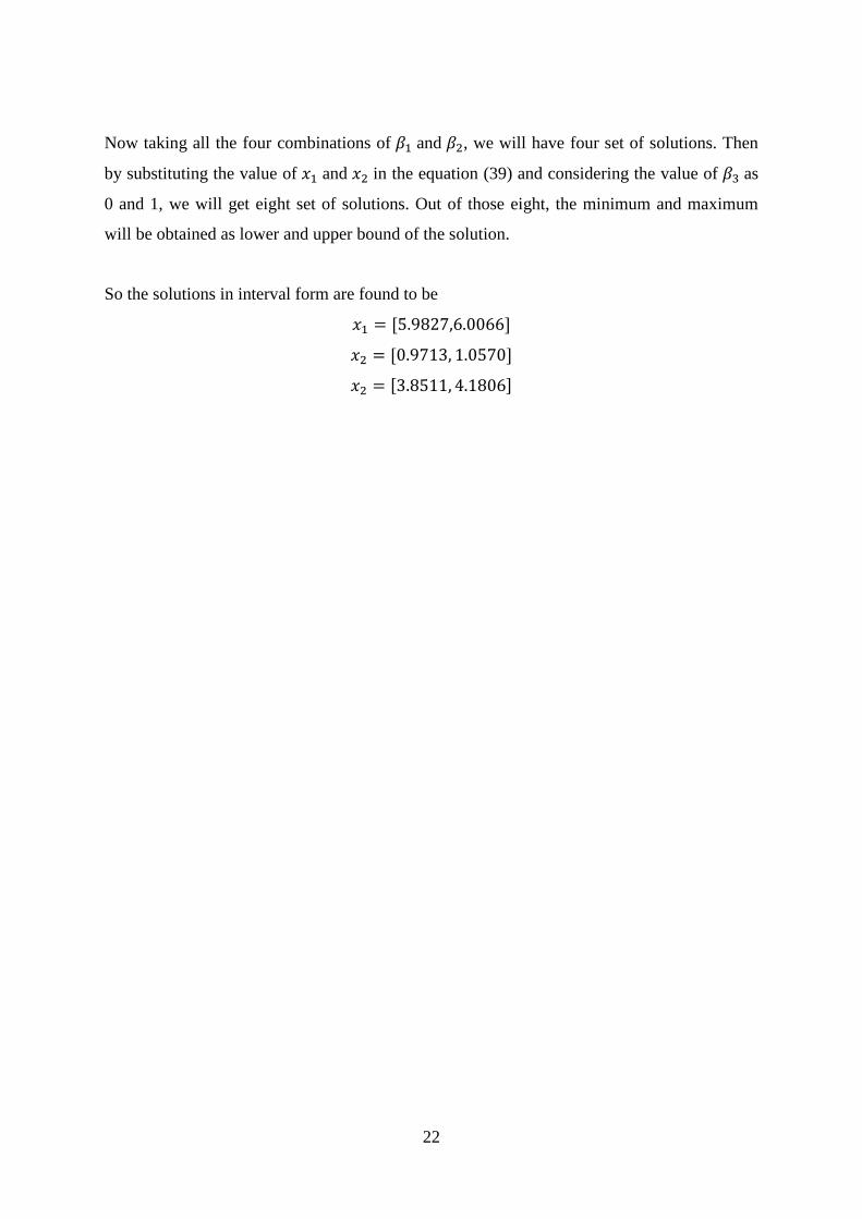
22

Now taking all the four combinations of 𝛽1 and 𝛽2, we will have four set of solutions. Then

by substituting the value of 𝑥1 and 𝑥2 in the equation (39) and considering the value of 𝛽3 as

0 and 1, we will get eight set of solutions. Out of those eight, the minimum and maximum

will be obtained as lower and upper bound of the solution.

So the solutions in interval form are found to be

𝑥1 = [5.9827,6.0066]

𝑥2 = [0.9713, 1.0570]

𝑥2 = [3.8511, 4.1806]

23

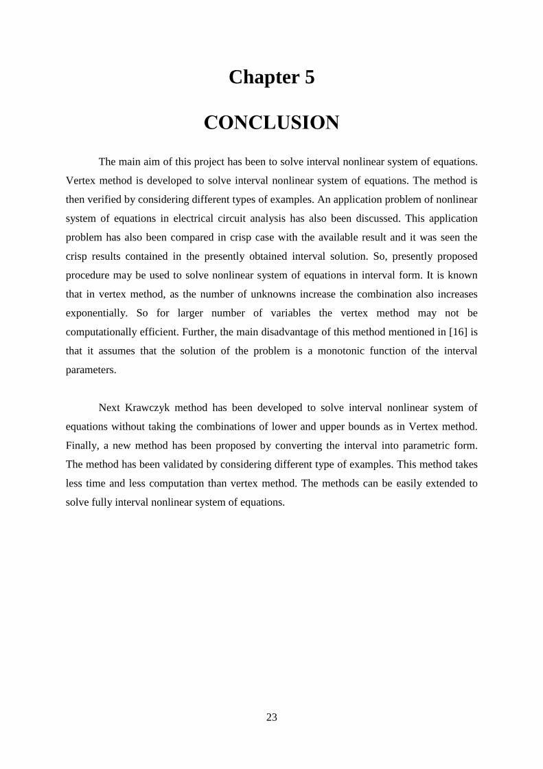
Chapter 5

CONCLUSION

The main aim of this project has been to solve interval nonlinear system of equations.

Vertex method is developed to solve interval nonlinear system of equations. The method is

then verified by considering different types of examples. An application problem of nonlinear

system of equations in electrical circuit analysis has also been discussed. This application

problem has also been compared in crisp case with the available result and it was seen the

crisp results contained in the presently obtained interval solution. So, presently proposed

procedure may be used to solve nonlinear system of equations in interval form. It is known

that in vertex method, as the number of unknowns increase the combination also increases

exponentially. So for larger number of variables the vertex method may not be

computationally efficient. Further, the main disadvantage of this method mentioned in [16] is

that it assumes that the solution of the problem is a monotonic function of the interval

parameters.

Next Krawczyk method has been developed to solve interval nonlinear system of

equations without taking the combinations of lower and upper bounds as in Vertex method.

Finally, a new method has been proposed by converting the interval into parametric form.

The method has been validated by considering different type of examples. This method takes

less time and less computation than vertex method. The methods can be easily extended to

solve fully interval nonlinear system of equations.

24

REFERENCES

[1] P. Sevastjanov, L. Dymova, “A new method for solving interval and fuzzy equations:

Linear case”, Information Sciences 179, pp. 925–937, 2009.

[2] K Madsen, “On the solution of nonlinear equations in interval arithmetic”, BIT, 13,

pp. 428-433, 1973.

[3] Roman E. Moore, “A test for existence of solutions to nonlinear systems”, SIAM J.

Numer. Anal., 14(4): pp. 611-615, 1977.

[4] Roman E. Moore, “A computational test for convergence of iterative methods for

nonlinear systems”, SIAM J. Numer. Anal., 15(6): pp. 1194-1196, 1978.

[5] S. Chakraverty, S. Nayak, “Fuzzy finite element method for solving uncertain heat

conduction problems”, Coupled Systems Mechanics, Vol. 1, No. 4, pp. 345-360,

2012.

[6] S. Chakraverty, D. Behera, “Fuzzy system of linear equations with crisp coefficients”,

Journal of intelligent and fuzzy systems, Vol. 25, Issue 1, pp. 201-207, 2013.

[7] D. Behera, S. Chakraverty, “New approach to solve fully fuzzy system of linear

equations using single and double parametric form of fuzzy numbers”, Sadhana Vol.

40, Part 1, Indian Academy of Sciences, pp. 35–49, 2015.

[8] Ramon E. Moore, R. Baker Kearfott, Michael J. Cloud, “Introduction to Interval

Analysis” Society for Industrial and Applied Mathematics (SIAM) Philadelphia,

2009.

[9] Gotz Alefeld, Jiirgen Herzberger, “Introduction to Interval Computations”, Academic

Press, 1983.

[10] Curtis F. Gerald, Patrick O. Wheatley, “Applied numerical analysis”, Seventh edition,

Pearson education

[11] R. Rama Bhat, S. Chakraverty, “Numerical Analysi in Engineering”, Aplha science

international Ltd, revised edition 2007.

[12] W. Dong, H. Shah, “Vertex method for computing functions of fuzzy variables”,

Fuzzy Set. Syst., 24(1), pp. 65-78, 1987.

[13] Rudolf Krawczyk. Newton-Algorithmen zur Bestimmung von Nullstellen mit

Fehlerschranken. Interner Bericht des Inst. für Informatik 68/6, Universität Karlsruhe,

1968. Computing, 4: pp. 187–201, 1969.

25

[14] M. Arounassalame, “Analysis of nonlinear electrical circuits using Bernstein

polynomials”, International Journal of Automation and Computing, 9(1), pp. 81-86,

2012.

[15] L. Kolev. An interval method for global nonlinear analysis. IEEE Transactions on

Circuits and Systems I: Fundamental Theory and Applications, vol. 45, no. 5, pp.

675–683, 2000.

[16] Bart M. Nicolai, Jose A. Egea, Nico Scheerlinck, Julio R. Banga, Ashim K. Datta,

“Fuzzy finite element analysis of heat conduction problems with uncertain

parameters”, Journal of Food Engineering 103, pp.38–46, 2011.

26

LIST OF PUBLICATIONS

Sandeep Nayak, S. Chakraverty, “Numerical Solution of Interval Nonlinear System of

Equations”, International Conference of Computational Intelligence & Network

Engineering 2015, IEEE CPS, DOI: 10.1109/CINE.2015.43

Sandeep Nayak, S. Chakraverty, “The Krawczyk Method for Solving Interval Nonlinear

System of Equations”, Best Presentation Award at 42nd Annual Conference by OMS

and A National Seminar on “Uncertain Programming”, 7-8th February 2015, at

Vyasanagar Autonomous College, Jajpur Road.