Automatica 47 (2011) 1868–1877

Contents lists available at SciVerse ScienceDirect

Automatica

journal homepage: www.elsevier.com/locate/automatica

Numerical solution of a conspicuous consumption model with constantcontrol delay✩

Tony Huschto a,∗, Gustav Feichtinger b, Richard F. Hartl c, Peter M. Kort d,e, Sebastian Sager a,Andrea Seidl ba Interdisciplinary Center for Scientific Computing, University of Heidelberg, Germanyb Institute for Mathematical Methods in Economics, Vienna University of Technology, Austriac Department of Business Administration, University of Vienna, Austriad Department of Econometrics & Operations Research and CentER, Tilburg University, Netherlandse Department of Economics, University of Antwerp, Belgium

a r t i c l e i n f o

Article history:Received 30 September 2010Received in revised form11 January 2011Accepted 5 March 2011Available online 25 June 2011

Keywords:Optimal controlOptimization under uncertaintiesControl delaysEconomic systemRecession

a b s t r a c t

We derive optimal pricing strategies for conspicuous consumption products in periods of recession.To that end, we formulate and investigate a two-stage economic optimal control problem that takesuncertainty of the recession period length and delay effects of the pricing strategy into account.

This non-standard optimal control problem is difficult to solve analytically, and solutions depend onthe variable model parameters. Therefore, we use a numerical result-driven approach. We propose astructure-exploiting direct method for optimal control to solve this challenging optimization problem.In particular, we discretize the uncertainties in the model formulation by using scenario trees and targetthe control delays by introduction of slack control functions.

Numerical results illustrate the validity of our approach and show the impact of uncertainties anddelay effects on optimal economic strategies. During the recession, delayed optimal prices are higher thanthe non-delayed ones. In the normal economic period, however, this effect is reversed and optimal priceswith a delayed impact are smaller compared to the non-delayed case.

© 2011 Elsevier Ltd. All rights reserved.

1. Introduction

We are interested in optimal pricing strategies for conspicuousconsumption products in periods of recession, such as the creditcrunch recession that started in 2007. Besides a reduction indemand, which is quite usual for a recession, in the credit crunchrecession capital markets cease to function. Hence firms cannotborrow or issue new shares to finance their operations. They needto self-finance their investments (Economist, 2008):

‘‘. . . the only option is to try to ride out the recession. But companiescan do this only if they have enough liquidity. . . ’’.

✩ This research was supported by the Heidelberg Graduate School Mathematicaland Computational Methods for the Sciences and the Austrian Science Fund (FWF)under Grant P21410-G16, which is gratefully acknowledged. This paper was notpresented at any IFAC meeting. This paper was recommended for publication inrevised form by Associate Editor Qing Zhang under the direction of Editor BerçRüstem.∗ Corresponding author. Tel.: +49 6221 548809; fax: +49 6221 545444.

E-mail addresses: tony.huschto@iwr.uni-heidelberg.de (T. Huschto),gustav@eos.tuwien.ac.at (G. Feichtinger), richard.hartl@univie.ac.at (R.F. Hartl),kort@uvt.nl (P.M. Kort), sebastian.sager@iwr.uni-heidelberg.de (S. Sager),aseidl@eos.tuwien.ac.at (A. Seidl).

0005-1098/$ – see front matter© 2011 Elsevier Ltd. All rights reserved.doi:10.1016/j.automatica.2011.06.004

For conspicuous goods demand does not only depend onprice, but in addition it depends on the good’s reputation, whichincreases in price. The product’s reputation as being expensiveallows people to signal their wealth to observers, which inturn increases the reputation of the consumer. Examples ofconspicuous goods are luxury hotels (Times, 2008), expensive cars,or fashionable clothes. The topic of how to price conspicuous goodsis treated in Amaldoss and Jain (2005a,b) and Kort, Caulkins, Hartl,and Feichtinger (2006).

This paper treats themanagement of conspicuous goods duringthe credit crunch recession. The conspicuous goods’ manager facesthe following trade off. To keep future demand at a high levelthe manager likes to keep the price of its conspicuous good high.However, during the recession demand as such is low and pricingthe good high makes demand even lower. This has detrimentaleffects for the firm’s cash flow, which can bring it into bankruptcyproblems, because during the recession capital markets do notfunction so that the firmneeds to have a positive cash level in orderto prevent bankruptcy. In Caulkins and Feichtinger et al. (2010) andCaulkins et al. (2011) this problem was extensively analyzed.

The present paper extends Caulkins and Feichtinger et al.(2010) and Caulkins et al. (2011) by establishing a new numericalmethodology and by considering a delayed effect of the current

T. Huschto et al. / Automatica 47 (2011) 1868–1877 1869

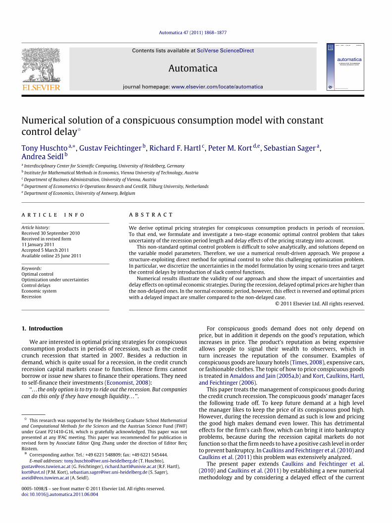
Fig. 1. Stages [t0, τ ] and [τ , tf] of the recession model.

price on the firm’s reputation. This implies that the good’sreputation, which has been built up in the past, is not immediatelyaffected by a price decrease. It takes some time for consumers toget used to the new situation, before a price change really starts tohave an effect on the good’s reputation.

The very first paper including a delay in an economic modelwas Kalecki (1935) treating a descriptive business cycle model.Much later, El-Hodiri, Loehman, andWhinston (1972) analyzed anoptimal growth model with time lags. Starting with the ninetiesseveral so-called time-to-build (investment gestation lag) modelshave been dealt with. Continuous-time deterministic optimalgrowth models have been enriched by assuming that productionoccurs with a delay while new capital is installed; see Asea andZak (1999), Boucekkine, Licandro, Puch, and del Rio (2005), Bambi(2008), Bambi, Fabbri, and Gozzi (2009) and Collard, Licandro,and Puch (2008). The methodological background are functionaldifferential equations; for a modified version of Pontryagin’sMaximum Principle compare Kolmanovskii and Myshkis (1992).Additionally, in Winkler (2004) and Winkler, Brandt-Pollmann,Moslener, and Schlöder (2005) some related results are presented.In Collard et al. (2008) economicmodels characterized by advancedor delayed time arguments in both the states and controlsare discussed. The authors present an algorithm combining themethod of steps and a specially tailored shooting method.

It turns out that introducing this delayed effect has considerablequalitative implications for pricing the conspicuous good. Inparticular, the delayed consumer reaction makes that it is optimalfor the firm to set a higher price during the recession and a lowerone during the normal period.

We formulate and investigate a two-stage economic optimalcontrol problem that takes uncertainty of the recession periodlength and delay effects of the pricing strategy into account. Thisnon-standard optimal control problem is difficult to solve analyt-ically, and solutions depend on the variable model parameters.Therefore we use a numerical result-driven approach. We proposea structure-exploiting direct method for optimal control to solvethis challenging optimization problem. In particular, we discretizethe uncertainties in the model formulation by using scenario treesand target the control delays by introduction of slack control func-tions.

The paper is organized as follows: In Section 2 we take acloser look at the model. We specify the underlying dynamics foreach of the economic stages and deduce the objective function.In Section 3 we first collect the algorithmic approaches used tosolve a standardmulti-stage optimal control problem numerically.Then we reformulate the model using a scenario tree approachand rearrange the emerging scheme to improve performanceand simplify the incorporation of the delay via slack controlfunctions. Section 4 treats analytical and numerical results andtheir economic interpretations in detail.

2. Model formulation

We consider an economic setting with a recession periodfollowed by a normal economic period. In the following, the valueτ will denote the endpoint of the crisis, compare Fig. 1.

The dynamics of our model includes two states. The brandimage A of the firm evolves in both periods according to thedifferential equation

A(t) = κ(γ p(t − σ) − A(t)) (1)

with a possible constant control delayσ ≥ 0 in the dynamics of thereputation A(·), retarding the connection between changing theprice p(·) and its consequence on the development of A(·). Eq. (1)covers that, as usual with conspicuous goods, the reputation of thebrand goes up with the price, which works positively on demand.Compared to the literature, the delay is a new feature, whichcaptures the fact that consumers first have to get used to a newsituation before they adjust their purchase decisions. In particular,if a good is known to be exclusive, a sudden price reduction atfirst instance does not change this perception. However, after awhile consumers ‘‘forget’’ the old situation, implying that they startrecognizing that the good is less exclusive, and reputation starts todecrease. Note that if the recession ends at time τ , we still havethe direct influence of the price set during the final time intervalof length σ of the recession. For a fixed price p Eq. (1) yields asteady state of A = γ p. The available cash B(·) depends on thegains p(·) D(·), fixed costs C , and the short-time interest δ, leadingto

B(t) = p(t)D(A(t), p(t)) − C + δB(t).

Therein the demandD is driven by the brand image and the pricingstrategy p(·), which is the control of our problem. It is essentiallyinfluenced by the economic stage, i.e., in the normal period (N) wehave

DN(A(t), p(t)) = m −p(t)A(t)β

, (2a)

whereas in the recession (R) demand is reduced to

DR(A(t), p(t)) = DN(A(t), p(t)) − α. (2b)

The positive constant α measures the strength of the crisis, theparameter 0 < β < 1 is given, andm corresponds to the potentialmarket size.

The objective of the company is tomaximize the expected valueof profit over the finite or infinite time horizon [0, tf] of interest.The profit is composed of two parts: the gains of the normaleconomic period (τ , tf] and an impulse dividend of the cash reserveat the end of the recession phase, B(τ ). This dividend is includedas the capital market is assumed to become functional again inthe normal economic period and firms can freely borrow and lendcash there. Thus, the firm does not need a positive B(·) on (τ , tf].For a fixed τ and a given discount rate r , the objective function iscalculated as

Φ(τ ) := e−rτB(τ ) +

∫ tf

τ

e−rt (p(t)DN(A(t), p(t)) − C) dt, (3)

being the sum of these two components, resulting in the optimalcontrol problem

maxp(·)

Φ(τ )

s.t. A(t) = κ(γ p(t − σ) − A(t)), t ∈ [0, tf],p(t) = η(t), t ∈ [−σ , 0],B(t) = p(t)DR(A(t), p(t)) − C + δB(t), t ∈ [0, τ ],A(0) = A0, B(0) = B0,0 ≤ DR/N(A(t), p(t)), t ∈ [0, tf],p(t) ≥ 0, t ∈ [0, tf],B(t) ≥ 0, t ∈ [0, τ ]

(4)

with DR/N(A(t), p(t)) given as in (2) and B(t) negligible in thenormal period (τ , tf]. However, typically the recession length τis not known beforehand to decision makers. An individual firmalso has no influence on when the recession ends. Therefore,we assume that the length of the recession period τ is anexponentially distributed randomvariable. The goal is tomaximizethe expectation value of the net present value (NPV) at time τ , i.e.,

1870 T. Huschto et al. / Automatica 47 (2011) 1868–1877

the objective function Φ weighted by the exponential probabilitydensity function with rate parameter λ,

maxp(·)

E [NPV(τ )] := maxp(·)

∫ tf

0λ e−λτ Φ(τ ) dτ (5)

subject to the constraints given in (4) for all 0 ≤ τ ≤ tf.This problem is a non-standard optimal control problem

in the sense that uncertainty and control delays are present,making analytical investigations difficult.1 Therefore, we proposea different approach in the next section.

3. Numerical treatment

We propose to use reformulations to transfer the optimalcontrol problem (5) into a more standard form that can beefficiently solved. In Section 3.1 we present such a standard multi-stage formulation and give references to Bock’s direct multipleshooting method. In Section 3.2 we present a discretization of theuncertainty, and in Section 3.3 a reformulation of the time delays.In both cases alternatives are discussed.

3.1. The direct multiple shooting approach

Efficient numerical methods have been developed to solvemulti-stage, nonlinear optimal control problems of the followingform

maxxi(·),ui(·),q,ti

M−1−i=0

∫ ti+1

tiLi(xi(t), ui(t), q) dt + Ei(x(ti+1), q)

(6a)

s.t. xi = fi(xi(t), ui(t), q), (6b)xi+1(ti+1) = ftr,i(xi(ti+1), q), (6c)

0 ≤ ci(xi(t), ui(t), q) (6d)0 = req(x0(t0), x1(t1), . . . , q), (6e)

0 ≤ rineq(x0(t0), x1(t1), . . . , q), (6f)

with t ∈ [ti, ti+1] and i = 0, . . . ,M − 1. The optimizationproblem (6) couples M model stages via explicit transitions (6c)and interior point constraints (6e)–(6f). The differential states xi :

[t0, tM ] → Rnxi and the control functions ui : [t0, tM ] → Rnui

and control values q ∈ Rnq need to be feasible for the path- andcontrol constraints (6d) and the ordinary differential equations(ODEs) (6b).

An overview of different methods can be found, e.g., in Binderet al. (2001). We propose to use Bock’s direct multiple shootingmethod to solve problems of type (6). It transforms the optimalcontrol problem into aNonlinear Program (NLP) by discretizing thespace of admissible control functions u(·) and the path constraints(6d). The solutions of the ODEs (6b) are obtained by a decoupledintegration on a multiple shooting grid, starting from artificialintermediate variables. Continuity of the differential states isassured by means of an inclusion of matching conditions into theNLP.

For details on this method we refer to Bock and Plitt (1984),Leineweber (1999) and Leineweber, Bauer, Bock, and Schlöder(2003). At this place we would only like to remind the reader ofone of the advantages of the direct multiple shooting method. Ascontrol functions, constraints and multiple shooting variables are

1 In Caulkins, Hartl, and Kort (2010) it is shown that an important class of modelswith delays can be transformed into equivalent problemswithout delays. However,the present model does not fit in this family. This is because the control p appearswith a delay in one state equation and without in the other one. Hence, it is notpossible to eliminate the delay using a time transformation.

discretized on a common time grid, the Hessian of the Lagrangianis block structured for linearly coupled point constraints r·(·). Fori = j we have

∇2L(w1, . . . , wN)

∂wi ∂wj= 0 (7)

for variable vectors wi that subsume all variables of the i-thmultiple shooting interval. This allows applyingBroyden–Fletcher–Goldfarb–Shanno (BFGS) updates to every single one of the N mul-tiple shooting blocks (Bock & Plitt, 1984). These high-rank updatestypically lead to a fast accumulation of higher order informationand thus to fast convergence (Nocedal & Wright, 2006). This fea-ture will become important in the context of the following refor-mulations of problem (5).

3.2. Discretizing the probability density function

To solve problem (5) at least approximatively, we need toreformulate it. We discretize the exponential distribution of therandom variable τ by defining a time grid

0 = τ0 < τ1 < · · · < τn < tf.

In the following, switches from recession period to normal stagewill only be possible at these times τi with i = 1 . . . n. The recessionends at τi with probability Pi. We use an equidistant discretization,resulting in a geometric distribution

Pi =

∫ τi

τi−1

λe−λtdt = e−λτi−1 − e−λτi , (8a)

for i = 1, . . . , n − 1, and

Pn = 1 −

n−1−j=1

Pj. (8b)

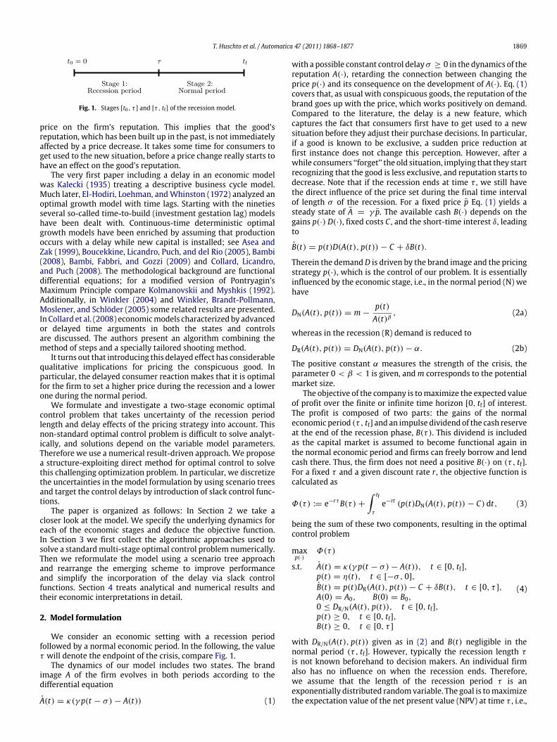
The discretized distribution can be used to reformulate themaximization of the expected value as a multi-stage optimalcontrol problem of type (6), by using a scenario tree. However,this formulation is not unique. One possibility is to use a staircase-like approach, increasing the number of variables as the numberof possible recession ends τi increases. This approach is illustratedschematically in Fig. 2 and results in M = n + 1 model stages,where n is the number of discretizations of the probability densityfunction. The dimensions nxi = 2 + i of differential states andnui = 1 + i of control functions, i = 0, . . . ,M − 1, are different onthe model stages. The transition functions (6c) are defined by

Ai,j(τi) = Ai−1,j(τi), 1 ≤ j ≤ i, (9a)

Ai,i+1(τi) = Ai−1,1(τi), (9b)

Bi,1(τi) = Bi−1,1(τi), (9c)

for all model stages i = 1, . . . , n − 1, and

An,n+1(τn) = An−1,1(τn). (9d)

At each τi one has to distinguish between transitions (9a), (9c) ofthe brand image A and the cash B for the ongoing recession and theinitialization (9b), (9d) of the additional differential states Ai,i+1 forthe normal period beginning at τi, compare Fig. 2.

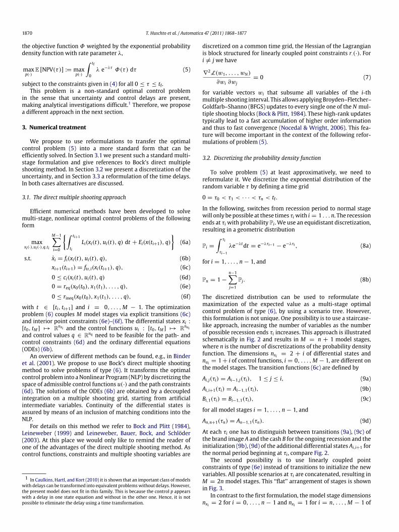
The second possibility is to use linearly coupled pointconstraints of type (6e) instead of transitions to initialize the newvariables. All possible scenarios at τi are concatenated, resulting inM = 2n model stages. This ‘‘flat’’ arrangement of stages is shownin Fig. 3.

In contrast to the first formulation, the model stage dimensionsnxi = 2 for i = 0, . . . , n − 1 and nxi = 1 for i = n, . . . ,M − 1 of

T. Huschto et al. / Automatica 47 (2011) 1868–1877 1871

Fig. 2. Controls and variables in the multi-stage formulation of problem (4) with associated probabilities and in a (R)ecession or a (N)ormal period.

Fig. 3. Rearranged scheme for the discretization of the random end time τ of the recession. Again, the symbols denote the (R)ecession and (N)ormal stage, as well as theappropriate probabilities.

differential states and nui = 1 for i = 0, . . . ,M − 1 of controls are(almost) constant. The coupled point constraints (6e) are given by

Ai,1(ti−n) = Ai−n−1,1(τi−n), n + 1 ≤ i ≤ 2n − 1. (10a)

The first n stages are recession periods with continuous transitionsof all states. They differ in the objective function. The transitionfrom the last recession stage n to the subsequent normal periodthat starts at t = τn is continuous, too. However, the model stagelengths of this approach vary. While all n recession stages have theconstant duration h = τi − τi−1, the n normal period stages have alength of tf − τi, i = 1, . . . , n.

Then we obtain for the staircase-like approach to discretize theprobability density function, k = 1, the objective function

Φ1i (τi, Ai,·(t), Bi−1,1(τi), p(t), Pi)

= Pie−rτiBi−1,1(τi) +

i−j=1

Pj

×

∫ τi+1

τi

e−rt p(t)DN(Ai,j+1(t), p(t)) − Cdt (11a)

for i = 1, . . . , n, the transition (tr) functions

f 1tr A,i(Ai−1,j(τi)) =

Ai−1,j(τi); 1 ≤ i ≤ n − 1, 1 ≤ j ≤ i,Ai−1,1(τi); 1 ≤ i ≤ n, j = i + 1, (11b)

f 1tr B,i(Bi−1,1(τi)) = Bi−1,1(τi), 1 ≤ i ≤ n − 1, (11c)

and the coupled point constraints functions

r1eq,i ≡ 0, (11d)

where Pi = (P1, P2, . . . , Pi).The concatenated approach, k = 2, is defined by the respective

functions

Φ2i (τi, An+i,1(t), Bi−1,1(τi), p(t), Pi) = Pi e−rτiBi−1,1(τi)

+ Pi

∫ tf

τi

e−rt p(t)DN(An+i,1(t), p(t)) − Cdt, (12a)

for i = 1, . . . , n,

f 2tr A,i(Ai−1,1(τi)) = Ai−1,1(τi), 1 ≤ i ≤ n, (12b)

f 2tr B,i(Bi−1,1(τi)) = Bi−1,1(τi), 1 ≤ i ≤ n − 1, (12c)

r2eq,i(Ai,1(ti−n), Ai−n−1,1(τi−n))

= Ai,1(ti−n) − Ai−n−1,1(τi−n), n + 1 ≤ i ≤ M − 1. (12d)

3.3. Reformulation of the time delays

In Brandt-Pollmann, Winkler, Sager, Moslener, and Schlöder(2008) two possibilities are given to reformulate an optimalcontrol problem with delayed equation of motion as in (4) into aninstantaneous problem.

The first approach splits the time horizon tf into m parts oflength σ and formulates the system dynamics separately on eachof the resulting intervals. By interpreting them as independentand introducing new state and control variables we can formulatea system of m differential equations on the time horizon [0, σ ].This can be used to reformulate the original optimal controlproblem. Furthermore, one has to introduce coupled boundaryconditions to ensure the continuity of the state variable. Theapproach may give additional insight from an analytical point ofview, compare Brandt-Pollmann et al. (2008). However, it requiresthe determination ofm− 1 control paths in the interval [0, σ ]. Forsmall values of the delay σ this results in a large number of stateand control functions.

Therefore, we prefer a different reformulation. We introduce asecond control function u2(t) = p(t) that denotes the unretardedcontrol at time t , whereas u1(t) = p(t − σ) characterizes thedelayed one. They are coupled via equalities u1(t) = u2(t − σ)for t ≥ σ and u1(t) = η(t − σ) for 0 ≤ t ≤ σ .

Taking either staircase (11) or flat (12) discretization ofuncertainty presented in the previous Section, k = 1, 2, we obtain

maxu1(·),u2(·)

n−i=1

Φki (τi, Aχk(i),·(t), Bi−1,1(τi), u2(t), Pi) (13a)

s.t. Ai,j(t) = κ(γ u1(t) − Ai,j(t)), t ∈ [0, tf],

1872 T. Huschto et al. / Automatica 47 (2011) 1868–1877

0 ≤ i ≤ M − 1, j ∈ Jk, (13b)Bi,1(t) = u2(t)DR(Ai,1(t), u2(t)) − C + δBi,1(t),

t ∈ [0, τi], 0 ≤ i ≤ n − 1, (13c)u1(t) = η(t − σ), t ∈ [0, σ ], (13d)u1(t) = u2(t − σ), t ∈ [σ , tf], (13e)A0,1(0) = A0, B0,1(0) = B0,

0 ≤ DR/N(Ai,j(t), u2(t)), t ∈ [0, tf], (13f)

u1(t) ≥ 0, u2(t) ≥ 0, t ∈ [0, tf], (13g)Bi,1(t) ≥ 0, t ∈ [0, τi], 1 ≤ i ≤ n − 1, (13h)

Ai,j(τi) = f ktr A,i(Ai−1,j(τi)), 1 ≤ i ≤ n, j ∈ Jk, (13i)

Bi,1(τi) = f ktr B,i(Bi−1,1(τi)), 1 ≤ i ≤ n − 1, (13j)

0 = rkeq,i(Ai,1(ti−n), Ai−n−1,1(τi−n)),

n + 1 ≤ i ≤ M − 1, (13k)

where χ1(i) := i, χ2(i) := n + i, J1 := {j | 1 ≤ j ≤ i + 1},J2 := {j | j = 1}.

This problem still contains a delayed term, but it is not apparentin the system dynamics anymore. It has moved to a constraint(13e) on the controls. This can be efficiently dealt with themultipleshooting method we introduced in Section 3.1 for the special caseof a constant delay.

4. Results

As suggested in Caulkins and Feichtinger et al. (2010) andCaulkins et al. (2011), we use the following set of parameters inour numerical treatment:

κ = 2.0, γ = 5.0, C = 7.5, δ = 0.05,m = 3.0, β = 0.5, r = 0.1, λ = 0.5,α1 = 0.7, α2 = 0.836, α3 = 1.25.

(14a)

The choice for parameters r , δ, and λ is based on the assumptionthat we measure time in years and that the expected duration ofthe recession is two years. We set β assuming that an increasein reputation will influence less and less customers. The morefashionable the product is, the more specialized is its marketniche. See Caulkins et al. (2011) for a motivation of the remainingparameters.

A key result of Caulkins et al. (2011) was that the authorswere able to distinguish three different types of recessionscorresponding to the severity of the demand reduction and theresulting optimal strategy. Following their results, the values ofthe parameter α indicate a mild (α1 = 0.7), intermediate (α2 =

0.836), and severe (α3 = 1.25) economic crisis.Due to the discretization of τ we need to further specify the last

possible endpoint of the recession,

τn = 20. (14b)

This implies that in this context the probability that the recessionpersists longer than that is low, i.e., P[τ > 20] = 4.54 · 10−5. Forthe control delay we choose

σ = 0.25. (14c)

To accomplish this, two equidistant discretization step lengths areapplied, first with n1 = 20, i.e., h = τi − τi−1 = 1.0, andn2 = 40, i.e., h = 0.5. Each of them is combinedwith four shootingnodes per time unit, i.e., per year. Then condition (13e) can beimplemented via interior point constraints applied on the shootingnodes.

For convenience, the overall final time tf is chosen to be

tf = 21 (years), (14d)

Table 1Different scenarios used for computational performance tests and visualizations.Note that some of these scenarios are used in both a delayed (σ = 0.25) andundelayed model (σ = 0), others in only one of them. In undelayed settings η isobsolete and denoted by ‘‘–’’.

Scenario n α A0 B0 η

1 20 0.7 10.0 5.0 –2 20 0.836 20.0 5.0 –3 20 1.25 100.0 100.0 –

4 40 0.7 10.0 5.0 7.4067855 40 0.7 0.1 5.0 4.2964606 40 0.7 10.0 2.0 7.0880017 40 0.7 AN

d 5.0 pNd8 40 0.7 AN

d 1.0 pNd9 40 0.7 AN

d 0.1 pNd10 40 0.836 0.1 10.0 3.91796211 40 0.836 0.1 10.0 3.512 40 0.836 0.1 10.0 3.013 40 0.836 0.1 10.0 2.514 40 0.836 20.0 5.0 8.15357515 40 0.836 0.1 8.0 3.91794816 40 0.836 25.0 3.5 8.67182417 40 0.836 AN

d 1.0 pNd18 40 0.836 0.1 7.05 –19 40 0.836 63.0 0.05 –20 40 0.836 0.1 9.8 3.521 40 0.836 73.5 0.1 12.517549

22 40 1.25 100.0 100.0 10.75130723 40 1.25 0.1 100.0 2.92461824 40 1.25 40.0 80.0 7.85520825 40 1.25 80.0 50.0 9.92293426 40 1.25 0.1 60 2.92461727 40 1.25 AN

d 50.0 pNd28 40 1.25 AN

d 70.0 –29 40 1.25 0.1 76.0 –30 40 1.25 AN

d 71.5 pNd31 40 1.25 0.1 79.5 2.924580

so that we definitely have a small normal period of one year in allpossible stages.

Finally, in the subsequent sections we provide some computa-tional results. They are obtained with the following combinationsof number of discretization points n, recession parameter α, initialvalues (A0, B0), and initial price paths η for the delayed model, cf.Table 1.

In Section 4.1 we analyze the computational performance ofthe various reformulations presented in the previous section.In Section 4.2 we derive some analytical insight into theproblem structure. More economic insight can be gained from thecomputational results in Section 4.3.

4.1. Computational performance

As discussed in Sections 3.2 and 3.3 different mathematicallyequivalent reformulations of the optimal control problem (4) exist.However, they are by no means equivalent from a computationalpoint of view.

Table 2 compares the computational performance of the twodifferent approaches to discretize the uncertainty. With thestaircase formulation (11) (Fig. 2) the overall time horizon isquite small. However, the number of state variables is increasedcompared to the concatenated arrangement, leading to moresteps of the error-controlled, adaptive integrator. More significant,however, is the impact of more blocks in the Hessian ofthe Lagrangian. They are used for high-rank updates, compareSection 3.1. This leads to a drastic increase in local convergenceand hence to a decrease of the number of sequential quadraticprogramming (SQP) iterations (Leineweber et al., 2003) and overallcomputation time, as can be seen in Table 2 for the case σ = 0.

T. Huschto et al. / Automatica 47 (2011) 1868–1877 1873

Table 2Comparison of the different schemes for discretizing τ , see (11), (12), and Figs. 2and 3, respectively. The results correspond to the undelayed case, i.e., σ = 0. Thefaster convergence of (12) (recognizable in SQP iterations and runtime) is due to thehigh-rank updates mentioned in Section 3.1. The scenarios are listed in Table 1.

Scenario Scheme (11) Scheme (12)# of SQP t (s) # of SQP t (s)

1 846 5259 51 13412 829 1312 35 8353 858 1411 102 2969

4 1254 67131 102 2144314 1716 93773 48 961522 915 47285 102 24163

Table 3Comparison of the size of the resulting NLP for the delayed and the undelayedmodel.

Undelayed model Delayed modeln = 20 n = 40 n = 20 n = 40

Discr. points 940 1840 940 1840Variables 3797 7437 4738 9278Eq. constraints 2855 5595 3797 7437Ineq. constraints 7594 14874 9476 18556

Table 4Number of iterations and CPU time for undelayed and delayed scenarios. Thecomputational effort is moderately higher, when delays are taken into account.

Scenario Undelayed model Delayed Model# of SQP t (s) # of SQP t (s)

6 71 14103 60 202387 102 24515 98 28422

16 70 12896 102 2878717 69 14796 82 2446624 81 18114 81 2216627 101 24456 101 29404

These results carry over to the case with σ > 0, therefore we willconcentrate on the formulation (12) visualized in Fig. 3.

As already observed in Brandt-Pollmann et al. (2008), thefirst approach suggested in Section 3.3 to handle time lags σ iscomputationally inferior to the second one, although it might beinteresting from an analytical point of view. E.g., for scenarios 4–12the number of 1800 additional state and 1799 control functionsneeds to be included. Therefore,wewill use the second formulationin the following for our calculations. Table 3 gives an overview overthe moderate increase in the dimension of the resulting nonlinearprogram.

Table 4 gives an indication of the computational expense forincluding delays. The main part of the computation is neededfor the condensing algorithm, see Bock and Plitt (1984) andLeineweber (1999), which is almost identical for both cases, asthe state dimension is independent of σ . The main extra cost issolving the quadratic programs, as the runtime depends cruciallyon the number of control variables. Therefore, asymptotically forσ > 0 getting smaller and smaller, the quadratic programming(QP) runtime will become more and more dominant.

4.2. Analytical results

We deduce analytical results that help us to obtain a betterinsight into the qualitative changes related to the introduction ofthe time lagσ .We investigate the steady state in the normal periodof our model (4) and compare it with the result of the undelayedcase, i.e., σ = 0.

The integral term of Φ(·) in (3) corresponds to the normaleconomic period, where the capital markets are working again andwe are not using the cash state B anymore. Let AN

d/nd and pNd/nddenote the normal period’s steady state brand image and price inthe (d)elayed and the u(nd)elayed case, respectively.

By using Pontryagin’s Maximum Principle (Grass, Caulkins,Feichtinger, Tragler, & Behrens, 2008) we calculate

ANnd =

γm(r + κ)

2(r + κ) − βκ

11−β

, pNnd =ANnd

γ. (15a)

In the model’s delayed version the maximum principle is farmore complex, see El-Hodiri et al. (1972). However, in the normalperiod the stationary state of the corresponding one-dimensionalproblem can be derived using the results in Winkler, Brandt-Pollmann, Moslener, and Schlöder (2003). We substitute

F(t) := F(A(t), p(t)) = p(t)m −

p(t)A(t)β

− C

and obtain the Hamiltonian

H = e−rtF(t) + µ(t + σ) · κγ p(t) − µ(t) · κA(t)

with the co-state variable µ(t). This induces the system

A(t) = κ(γ p(t − σ) − A(t))

p(t) =1

Fpp(t)

(r + κ)Fp(t) + κγ e−rσ FA(t + σ)

− FpA(t)A(t)

that directly gives us the stationary price pNd . Further on, it yields

(r + κ) erσ

κγ= −

FA(t + σ)

Fp(t)

and, therefore, the equality

(r + κ)erσ = −βκ(AN

d )1−β

γm − 2(ANd )1−β

that determines the stationary state of the brand image

ANd =

γm(r + κ) erσ

2(r + κ) erσ − βκ

11−β

, pNd =ANd

γ. (15b)

The latter result obviously includes the special case (15a). Ourparameters (14) determine the values

ANnd = 96.899414, pNnd = 19.379883, (16a)

ANd = 95.421259, pNd = 19.084252. (16b)

Those coincide with the numerical results we obtained. One cansee the impact of the delay very clearly. The benefit of keepingthe price up is obtained later in the delayed world, while thebenefit of reducing it (with instantaneous profit) is still obtainedimmediately.

In the recession period the verification and calculation of steadystates cannot be done this straightforwardly. Further on, the so-called weak Skiba curves2 play an important role. While theauthors of Caulkins and Feichtinger et al. (2010)were able to deriveseveral results of the non-delayed case analytically, for the delayedmodel this is impeded much more.

2 Also known as threshold or weak DNSS curve referring to early contributionsof Dechert and Nishimura (1983), Sethi (1977, 1979) and Skiba (1978); see alsoGrass et al. (2008). Weak Skiba refers to the threshold property of this curveseparating different long-term solutions. Which strategy has to be applied ishistory-dependent and, thus, particularly depends on the initial state values.

1874 T. Huschto et al. / Automatica 47 (2011) 1868–1877

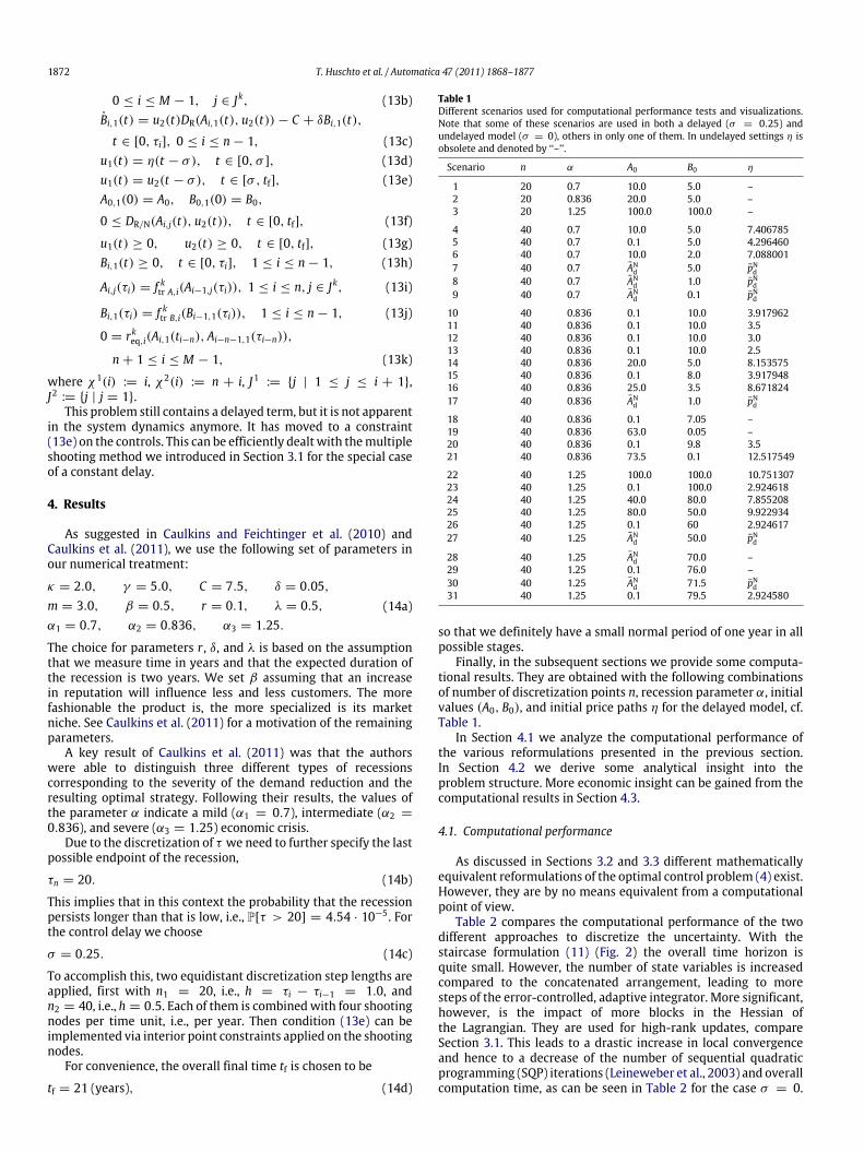
(a) Recession in [0, τn]. (b) Normal period in (τ1, tf].

Fig. 4. Exemplary price paths of (a) a recession period lasting until τn (using Scenario 22). During the recession pd > pnd holds, but the difference in between depends onthe size of the rate parameter λ. (b) A normal economic stage for the same scenario setting. By way of better illustration this figure shows price paths of a normal periodbeginning already at time τ1 . Note that neither λ nor the strength α of the recession have any influence on these paths. For comparison, ps shows the static optimizationprice.

4.3. Computational results

In our approach to discretize problem (4) we assume a finiteand discrete grid of possible switching times τi. We think thatthis transformation to the finite-time case is well justified, asthe influence of the errors caused by the discretization are small.The intervals between τi are short and the probability (8b) forswitching the stage at the last possible time τn is only marginallyhigher than it would be in the infinite case.

In Caulkins and Feichtinger et al. (2010) possible pricingstrategies in recession periods are explained depending on thevalue of α. Additionally, the impact of these pricing policies on thedevelopment of the reputation A and the cash B is depicted. In thedelayed world the behavior of the firm is qualitatively similar. In asevere crisis (α3 = 1.25) the brand image and/or cash required toavoid bankruptcy are particularly large. The milder the crisis is theless reputation/cash is needed. In all cases the cash state divergesto infinity if the firm survives with certainty.

The main result of our analysis of problem (4) is the relation

pd(t) > pnd(t), 0 ≤ t ≤ τ ,

pd(t) < pnd(t), τ ≤ t ≤ tf,(17)

which can be seen in Fig. 4.The optimal solution of the normal period follows the results

of Section 4.2. Due to the delay σ there is a less direct effect ofthe price pd on the dynamics of the brand image A. This reducesthe incentive to set a high price, as a lower price raises revenues,which consequently raises the value of the objective functionimmediately.

In the recession period, however, the opposite relation holds. Adirect consequence of this is visible in Figs. 5 and 6: The vertical lineindicating the divergence of the cash state B in an infinite horizonsetting is shifted to a value AR

d of reputation that is higher than therespective value AR

nd in the non-delayed case.While the negative effect of smaller revenueswith higher prices

(independent of the economic period) is the same for both thedelayed and the undelayed case, there are also two positive aspectsof increasing the price pd.

The first effect is that the brand image A will increase as wellduring the recession, implying that the bankruptcy probabilityreduces. This effect is stronger the less the delay σ is. Hence, thisfirst impact is the strongest in the non-delayed case.

Given that the recession will be terminated somewhere duringthe next time interval of duration σ , the second effect of increasing

pd is that the reputation goes up after the recession, implying thatthe revenue of the normal period rises. This effect occurs with theprobability P[τ ∈ [t, t + σ ]] that the recession will be over duringthe next interval of length σ , hence, it is stronger the larger thedelay is. But it is completely absent in the undelayed case.

According to the first effect, which is comparable to the impactin the normal period, it will hold that pd < pnd then. The secondeffect will imply the opposite relation during the recession stage.Note that this second impact only occurswith P[τ ∈ [t, t+σ ]], i.e.,it depends on the size of σ and the probability density function.

In our case (with σ = 0.25) the second effect dominates,meaning that the mentioned probability is large enough. Forthe first effect to dominate we have to decrease this probabilityby either reducing the time lag or end of recession probabilityparameter λ. The results of the latter possibility can be seen inFig. 4a.

In a more vivid way we can interpret this second effect byassuming that the crisis ends at time τ . In the undelayed case thefirm can start building up their reputation immediately after therealization of τ by charging higher prices (supposing that it hassurvived). The effect on A comes directly. If σ > 0 the impact ofrising prices after τ only starts to have a positive outcome fromtime τ + σ onwards. In the initial phase of the normal period[τ , τ + σ ] the demand is directly influenced by the price set in thelast interval of the recession. Hence, increasing prices in [τ −σ , τ ]

leads to a higher reputation σ time units later. That is, the demandis also higher in the period [τ , τ + σ ], which generates higherrevenues during the first phase of the normal period. As the firmdoes not know beforehand when the recession will be over, thereis always a positive probability that the current time t is locatedin the period [τ − σ , τ ]. Keeping this in mind, the firm has anadditional incentive to keep prices up in recession periods whena delay is apparent, avoiding damaging the reputation too much.Otherwise their product will still perceived to be comparativelycheap for some time period after the recession is over.

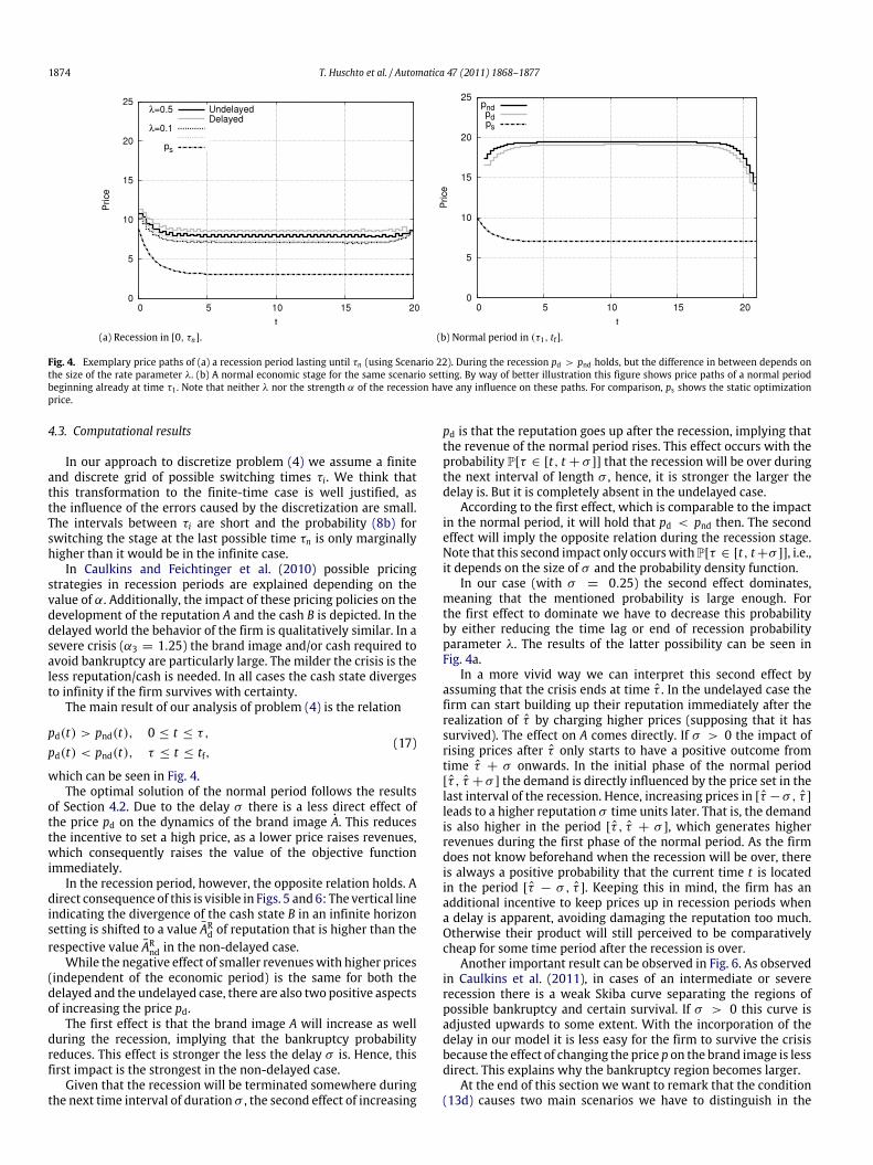
Another important result can be observed in Fig. 6. As observedin Caulkins et al. (2011), in cases of an intermediate or severerecession there is a weak Skiba curve separating the regions ofpossible bankruptcy and certain survival. If σ > 0 this curve isadjusted upwards to some extent. With the incorporation of thedelay in our model it is less easy for the firm to survive the crisisbecause the effect of changing the price p on the brand image is lessdirect. This explains why the bankruptcy region becomes larger.

At the end of this section we want to remark that the condition(13d) causes two main scenarios we have to distinguish in the

T. Huschto et al. / Automatica 47 (2011) 1868–1877 1875

a b

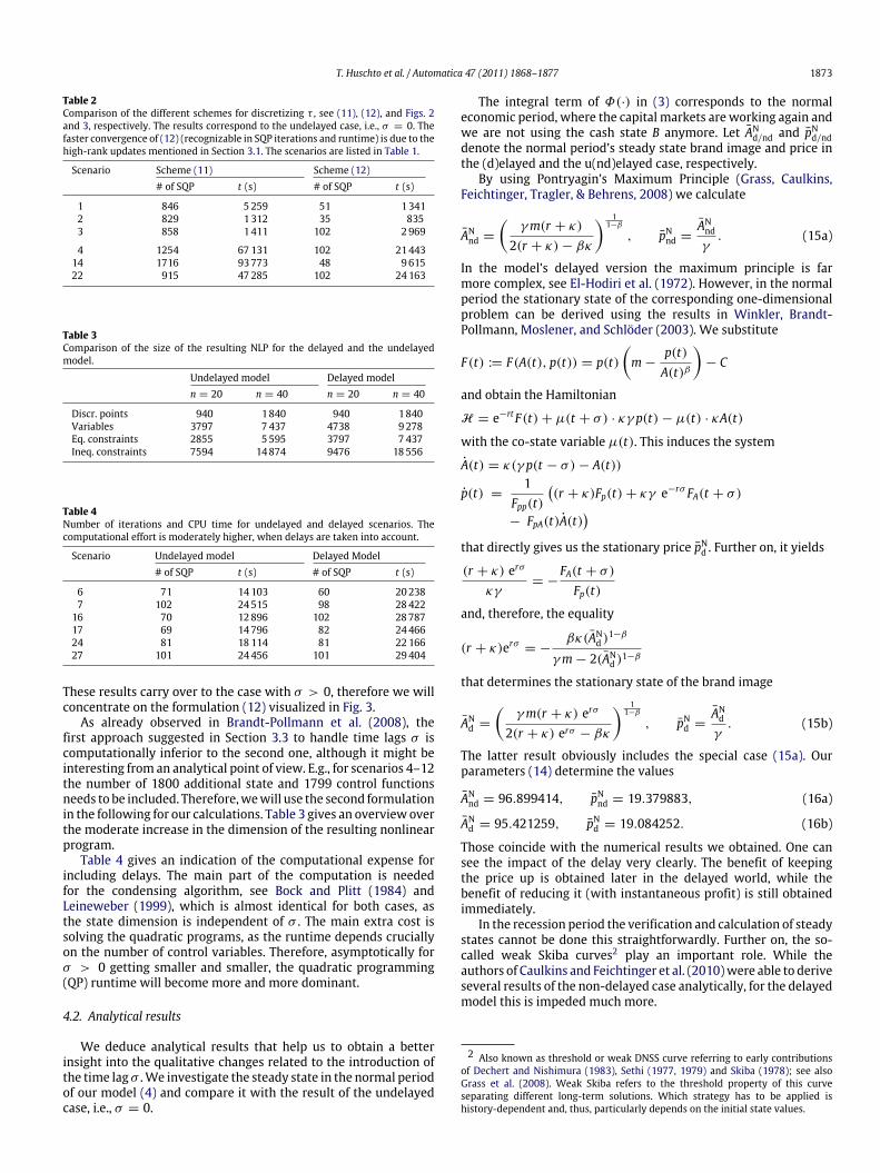
Fig. 5. Evolution of optimal trajectories over time in a phase diagram with brand image A(·) and capital B(·). They start in (A0, B0) according to Table 1 and evolve until(A(τn), B(τn)). Optimal solutions of a delayed (σ = 0.25) and the undelayed (σ = 0) model are shown for a mild recession (α1 = 0.7), if we assume that for t ∈ [−σ , 0](a) the recession has been present (Scenarios 4–6 (from top to bottom)), (b) a steady state normal economic period existed, i.e., A0 = AN

d , η = pNd (Scenarios 7–9). Due to theintroduction of the delay the recession’s steady state of the brand image AR

d (and correspondingly pRd) is greater than in the undelayed case.

(a) α2 = 0.836. (b) α3 = 1.25.

Fig. 6. Phase diagram as in Fig. 5a for an intermediate and severe recession. (a) Scenarios 10, 14–16, (b) Scenarios 22–26. In analogy to weak Skiba curves, the dotted linesbased on Scenarios (a) 18–21, (b) 28–31 indicate the initial values which separate the state space into the ones (above) that do not lead to bankruptcy and the ones (below)that do. After the introduction of the time lag σ the bankruptcy region becomes larger. This results in an upwards-adjustment of the weak Skiba curve in the delayed case.

delayed model. The economic stage that is apparent in the timeprior to the planning period [0, tf] can either be a normal or arecession stage. We consider two slightly simplified cases.

In the first one we assume a steady state corresponding tothe normal economic period in the interval [−σ , 0], i.e., wehave already one ‘‘switching’’ occurrence at the beginning of thehorizon. We initialize the retarded control with η = pNd and thebrand image with A0 = AN

d . Then the system evolves as shown inFig. 5b. The non-smooth behavior of the trajectories there is quitenatural. At t = 0 the recession begins and the demand is reducedimmediately due to the influence of α. Hence, prices will drop andthe firm’s cash decreases. However, the brand image in the timeinterval [0, σ ] develops according to the high steady state pricepNd , i.e., it remains at its level. Only thereafter the condition (13e)becomes active and the reputation reacts to the lower prices.

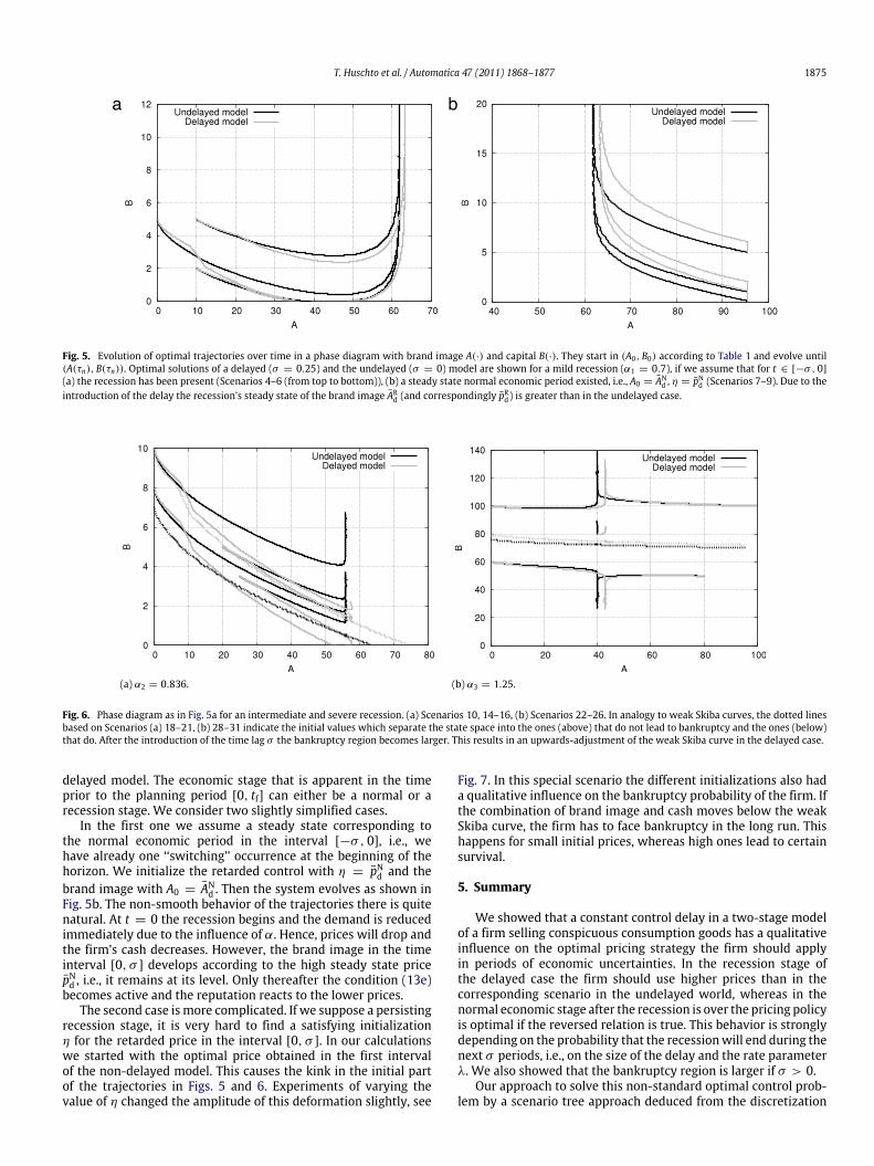
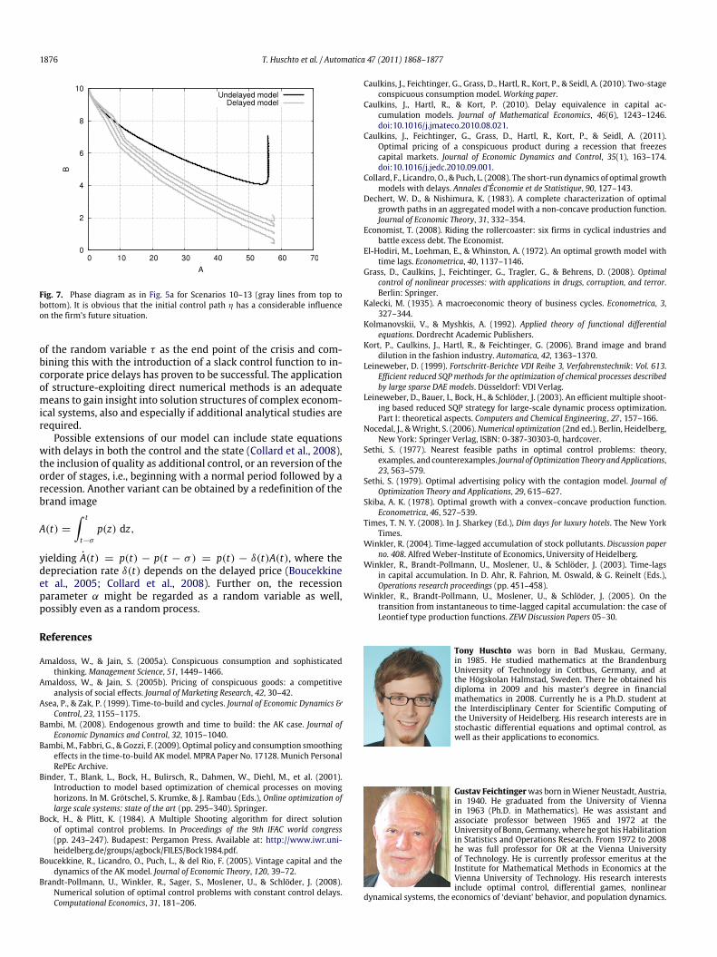
The second case ismore complicated. If we suppose a persistingrecession stage, it is very hard to find a satisfying initializationη for the retarded price in the interval [0, σ ]. In our calculationswe started with the optimal price obtained in the first intervalof the non-delayed model. This causes the kink in the initial partof the trajectories in Figs. 5 and 6. Experiments of varying thevalue of η changed the amplitude of this deformation slightly, see

Fig. 7. In this special scenario the different initializations also hada qualitative influence on the bankruptcy probability of the firm. Ifthe combination of brand image and cash moves below the weakSkiba curve, the firm has to face bankruptcy in the long run. Thishappens for small initial prices, whereas high ones lead to certainsurvival.

5. Summary

We showed that a constant control delay in a two-stage modelof a firm selling conspicuous consumption goods has a qualitativeinfluence on the optimal pricing strategy the firm should applyin periods of economic uncertainties. In the recession stage ofthe delayed case the firm should use higher prices than in thecorresponding scenario in the undelayed world, whereas in thenormal economic stage after the recession is over the pricing policyis optimal if the reversed relation is true. This behavior is stronglydepending on the probability that the recessionwill end during thenext σ periods, i.e., on the size of the delay and the rate parameterλ. We also showed that the bankruptcy region is larger if σ > 0.

Our approach to solve this non-standard optimal control prob-lem by a scenario tree approach deduced from the discretization

1876 T. Huschto et al. / Automatica 47 (2011) 1868–1877

Fig. 7. Phase diagram as in Fig. 5a for Scenarios 10–13 (gray lines from top tobottom). It is obvious that the initial control path η has a considerable influenceon the firm’s future situation.

of the random variable τ as the end point of the crisis and com-bining this with the introduction of a slack control function to in-corporate price delays has proven to be successful. The applicationof structure-exploiting direct numerical methods is an adequatemeans to gain insight into solution structures of complex econom-ical systems, also and especially if additional analytical studies arerequired.

Possible extensions of our model can include state equationswith delays in both the control and the state (Collard et al., 2008),the inclusion of quality as additional control, or an reversion of theorder of stages, i.e., beginning with a normal period followed by arecession. Another variant can be obtained by a redefinition of thebrand image

A(t) =

∫ t

t−σ

p(z) dz,

yielding A(t) = p(t) − p(t − σ) = p(t) − δ(t)A(t), where thedepreciation rate δ(t) depends on the delayed price (Boucekkineet al., 2005; Collard et al., 2008). Further on, the recessionparameter α might be regarded as a random variable as well,possibly even as a random process.

References

Amaldoss, W., & Jain, S. (2005a). Conspicuous consumption and sophisticatedthinking.Management Science, 51, 1449–1466.

Amaldoss, W., & Jain, S. (2005b). Pricing of conspicuous goods: a competitiveanalysis of social effects. Journal of Marketing Research, 42, 30–42.

Asea, P., & Zak, P. (1999). Time-to-build and cycles. Journal of Economic Dynamics &Control, 23, 1155–1175.

Bambi, M. (2008). Endogenous growth and time to build: the AK case. Journal ofEconomic Dynamics and Control, 32, 1015–1040.

Bambi,M., Fabbri, G., & Gozzi, F. (2009). Optimal policy and consumption smoothingeffects in the time-to-build AKmodel. MPRA Paper No. 17128. Munich PersonalRePEc Archive.

Binder, T., Blank, L., Bock, H., Bulirsch, R., Dahmen, W., Diehl, M., et al. (2001).Introduction to model based optimization of chemical processes on movinghorizons. In M. Grötschel, S. Krumke, & J. Rambau (Eds.), Online optimization oflarge scale systems: state of the art (pp. 295–340). Springer.

Bock, H., & Plitt, K. (1984). A Multiple Shooting algorithm for direct solutionof optimal control problems. In Proceedings of the 9th IFAC world congress(pp. 243–247). Budapest: Pergamon Press. Available at: http://www.iwr.uni-heidelberg.de/groups/agbock/FILES/Bock1984.pdf.

Boucekkine, R., Licandro, O., Puch, L., & del Rio, F. (2005). Vintage capital and thedynamics of the AK model. Journal of Economic Theory, 120, 39–72.

Brandt-Pollmann, U., Winkler, R., Sager, S., Moslener, U., & Schlöder, J. (2008).Numerical solution of optimal control problems with constant control delays.Computational Economics, 31, 181–206.

Caulkins, J., Feichtinger, G., Grass, D., Hartl, R., Kort, P., & Seidl, A. (2010). Two-stageconspicuous consumption model.Working paper.

Caulkins, J., Hartl, R., & Kort, P. (2010). Delay equivalence in capital ac-cumulation models. Journal of Mathematical Economics, 46(6), 1243–1246.doi:10.1016/j.jmateco.2010.08.021.

Caulkins, J., Feichtinger, G., Grass, D., Hartl, R., Kort, P., & Seidl, A. (2011).Optimal pricing of a conspicuous product during a recession that freezescapital markets. Journal of Economic Dynamics and Control, 35(1), 163–174.doi:10.1016/j.jedc.2010.09.001.

Collard, F., Licandro, O., & Puch, L. (2008). The short-run dynamics of optimal growthmodels with delays. Annales d’Économie et de Statistique, 90, 127–143.

Dechert, W. D., & Nishimura, K. (1983). A complete characterization of optimalgrowth paths in an aggregated model with a non-concave production function.Journal of Economic Theory, 31, 332–354.

Economist, T. (2008). Riding the rollercoaster: six firms in cyclical industries andbattle excess debt. The Economist.

El-Hodiri, M., Loehman, E., & Whinston, A. (1972). An optimal growth model withtime lags. Econometrica, 40, 1137–1146.

Grass, D., Caulkins, J., Feichtinger, G., Tragler, G., & Behrens, D. (2008). Optimalcontrol of nonlinear processes: with applications in drugs, corruption, and terror.Berlin: Springer.

Kalecki, M. (1935). A macroeconomic theory of business cycles. Econometrica, 3,327–344.

Kolmanovskii, V., & Myshkis, A. (1992). Applied theory of functional differentialequations. Dordrecht Academic Publishers.

Kort, P., Caulkins, J., Hartl, R., & Feichtinger, G. (2006). Brand image and branddilution in the fashion industry. Automatica, 42, 1363–1370.

Leineweber, D. (1999). Fortschritt-Berichte VDI Reihe 3, Verfahrenstechnik: Vol. 613.Efficient reduced SQP methods for the optimization of chemical processes describedby large sparse DAE models. Düsseldorf: VDI Verlag.

Leineweber, D., Bauer, I., Bock, H., & Schlöder, J. (2003). An efficient multiple shoot-ing based reduced SQP strategy for large-scale dynamic process optimization.Part I: theoretical aspects. Computers and Chemical Engineering , 27, 157–166.

Nocedal, J., &Wright, S. (2006). Numerical optimization (2nd ed.). Berlin, Heidelberg,New York: Springer Verlag, ISBN: 0-387-30303-0, hardcover.

Sethi, S. (1977). Nearest feasible paths in optimal control problems: theory,examples, and counterexamples. Journal of Optimization Theory and Applications,23, 563–579.

Sethi, S. (1979). Optimal advertising policy with the contagion model. Journal ofOptimization Theory and Applications, 29, 615–627.

Skiba, A. K. (1978). Optimal growth with a convex–concave production function.Econometrica, 46, 527–539.

Times, T. N. Y. (2008). In J. Sharkey (Ed.), Dim days for luxury hotels. The New YorkTimes.

Winkler, R. (2004). Time-lagged accumulation of stock pollutants. Discussion paperno. 408. Alfred Weber-Institute of Economics, University of Heidelberg.

Winkler, R., Brandt-Pollmann, U., Moslener, U., & Schlöder, J. (2003). Time-lagsin capital accumulation. In D. Ahr, R. Fahrion, M. Oswald, & G. Reinelt (Eds.),Operations research proceedings (pp. 451–458).

Winkler, R., Brandt-Pollmann, U., Moslener, U., & Schlöder, J. (2005). On thetransition from instantaneous to time-lagged capital accumulation: the case ofLeontief type production functions. ZEW Discussion Papers 05–30.

Tony Huschto was born in Bad Muskau, Germany,in 1985. He studied mathematics at the BrandenburgUniversity of Technology in Cottbus, Germany, and atthe Högskolan Halmstad, Sweden. There he obtained hisdiploma in 2009 and his master’s degree in financialmathematics in 2008. Currently he is a Ph.D. student atthe Interdisciplinary Center for Scientific Computing ofthe University of Heidelberg. His research interests are instochastic differential equations and optimal control, aswell as their applications to economics.

Gustav Feichtingerwas born inWiener Neustadt, Austria,in 1940. He graduated from the University of Viennain 1963 (Ph.D. in Mathematics). He was assistant andassociate professor between 1965 and 1972 at theUniversity of Bonn, Germany,where he got hisHabilitationin Statistics and Operations Research. From 1972 to 2008he was full professor for OR at the Vienna Universityof Technology. He is currently professor emeritus at theInstitute for Mathematical Methods in Economics at theVienna University of Technology. His research interestsinclude optimal control, differential games, nonlinear

dynamical systems, the economics of ‘deviant’ behavior, and population dynamics.

T. Huschto et al. / Automatica 47 (2011) 1868–1877 1877

Richard F. Hartl holds a chair of Production and Opera-tions Management at the University of Vienna. He stud-iedmathematics at theUniversity of Technology inVienna,where he also obtained his Ph.D. Hewas Post-Doctoral fel-low at the University of Toronto and Assistant and Asso-ciate Professor at the University of Technology in Vienna.Prior to his present appointment he was professor at theOvG University in Magdeburg, Germany. He received sev-eral recognitions for his work including Senior Extramu-ral Fellow of the Center for Economic Research (CentER),University of Tilburg. His research interest involves appli-

cation of OR methods in Production and Operations Management as well as appli-cation of optimal control in economics and management.

Peter M. Kort was born in Zierikzee, the Netherlandsin 1961. He received a M.Sc. degree in 1984 from theErasmus University Rotterdam and a Ph.D. from TilburgUniversity in 1988. In 1991 he became research fellowof the Royal Netherlands Academy of Arts and Sciences.Currently he is full professor in Dynamic Optimization inEconomics and Operations Research at Tilburg Universityand Guest Professor at the University of Antwerp. Hismain research areas are applied optimal control, dynamicsof the firm, real options theory, and strategic industrialorganization, in which he published about 85 papers in

refereed international journals.

Sebastian Sager studied mathematics in Montpellierand Heidelberg. He obtained his Ph.D. in 2006 fromthe Universität Heidelberg. After a year as postdoctoralfellow in Madrid, he got a position as a Junior ResearchGroup leader at the Interdisciplinary Center for ScientificComputing in Heidelberg. He received the DissertationPrize of the German Operations Research Society in 2006and the Klaus Tschira Award for Achievements in PublicUnderstanding of Science in 2007. His main interestsare in mixed-integer nonlinear optimization and optimalcontrol.

Andrea Seidl was born in Vienna, Austria, in 1982. Shereceived a masters degree in ‘‘economics and computerscience’’ in 2005 and a Ph.D. degree in 2009 bothfrom the Vienna University of Technology. Currently sheworks as a postdoctoral research assistant at the Institutefor Mathematical Methods in Economics at the ViennaUniversity of Technology. Her research interests includeoptimal control and its applications, in particular multi-stage models.