Numerical Simulations of the ... - NUMECA International

Fourth International Symposium on Marine Propulsors smp’15, Austin, Texas, USA, June 2015

Numerical Simulations of the Cavitating and Non-Cavitating Flow around the Postdam Propeller Test Case

E. Guilmineau, G.B. Deng, A. Leroyer, P. Queutey, M. Visonneau, J. Wackers

LHEEA CNRS UMR 6598, Ecole Centrale de Nantes

BP 92101, 44321 Nantes Cedex, France

ABSTRACT In this paper, the cavitating performance and open water performance of the SMP'15 propeller are numerically simulated using the flow solver ISIS-CFD. A cavitation model based on a transport equation and the k-ω SST turbulence model are coupled in the flow solver. The thrust and torque coefficients are presented for the open water case. The pressure distribution on the propeller blades is also presented. For the cavitating case, the cavity surface is presented as well as the thrust and torque coefficients.

Keywords Propeller, Open water, Cavitation, Numerical simulation, ISIS-CFD, Oblique flow.

1 INTRODUCTION Numerous studies based on experiments or computations have been carried out to investigate propeller open water characteristics. Most studies only consider the case of a propeller in straight ahead flow. However, under real conditions, a working propeller operates behind a ship usually in a complex wake, so that the propeller shows quite different hydrodynamic performance. Moreover the consequence of the disturbance of the ship is that the angle of attack is different from blade to blade and the loads acting on the blades in axial direction is not symmetric.

Few authors have reported on hydrodynamic characteristics of a marine propeller in oblique flow. El Moctar and Bertram used a Reynolds-averaged Navier-Stokes (RANS) solver to investigate the flow around a four-bladed modern propeller at oblique angles up to 12°. They found that the forces oscillate and the frequency of the oscillations increases with the angle of attack. Krasilnikov et al. (2009) used an unsteady RANS method to investigate the blade forces acting on a podded propeller operating in oblique flow conditions. They found that blades of pulling propeller experience comparable amplitudes and load levels at positive and negative heading angles, being mainly affected by the crossflow. The amplitudes and load levels on the blades of a pushing propeller are different at positive and

negative headings due to the interaction of the propeller with the separated strut wake. Shamsi and Ghassemi (2013) evaluated the performance of a podded propulsor in straight and azimuting condition by using a RANS approach with Moving Reference Frame. They found that the propeller thrust coefficient and the torque coefficient increase with increasing yaw angles. Their results also indicate that side force coefficients increase with increasing yaw angle and velocity advance ratio. Dubbioso et al. (2013, 2014) analyzed the performance of the CNR-INSEAN E779A propeller model in oblique flow by unsteady RANS and dynamically overlapping grid approach. Their main focus is on hydrodynamic loads that act on a single blade. They also discuss the flow features around the propeller. Unfortunately, due to the lack of experiments in oblique flow conditions, they did not perform a validation of the numerical computations. Yao (2015) investigated the hydrodynamic performance of a 6-bladed propeller in oblique flow. The hydrodynamic forces and moment showed a good agreement with experimental data under no cavitation condition or under weak cavitation condition.

A propeller data in oblique flow was provided by SVA Postdam with well-defined cases and conditions for the SMP'15 Workshop on Cavitating Propeller Performance. The experiments datasets cover the open water characteristics and cavitation tests. The workshop for this propeller is organized in a "blind test" format that none of the participants knows the experiment results prior to the workshop. The numerical simulation will be performed with the ISIS-CFD flow solver and only the propeller in oblique flow in open water case and the cavitation observation in oblique flow will be investigated.

2 NUMERICAL METHOD The solver ISIS-CFD, available as a part of FINETM/Marine computing suite, is an incompressible unsteandy Reynolds-averaged Navier-Stokes method mainly devoted to marine applications. The method features several sophistical turbulence models: apart from the classical two-equation k-

ε and k-ω models, the anisotropic two-equation Explicit Algebraic Reynolds Stress Model (EARSM), as well as Reynolds Stress Transport Model (RSTM), are available, see Deng & Visonneau (1999) and Duvigneau et al. (2003). All models are available with wall-function or low-Reynolds near wall formulation. Hybrid LES (Large Eddy Simulation) turbulence models based on Detached Eddy Simulation (DES) are also implemented and have been validated on automotive flows characterized by large separations, see Guilmineau et al. (2011). Additionally, several cavitation models, such as the Merkle model, Sauer model or Kuntz mode, are available in the solver.

The solver is based on the finite volume method to build the spatial discretization of the transport equations. The unstructured discretization is faced-based. While all unknown variables are cell-centered, the system of equations used in the implicit time stepping procedure are constructed face by face and the contribution of each face is then added to the two cells next to the face. This technique poses no specific requirements on the topology of the cells. Therefore, the grid can be completely unstructured: cells with an arbitrary number of arbitrarily-shaped faces are accepted. Pressure-velocity coupling is enforced through a Rhie & Chow SIMPLE like method: at each time step, the velocity updates come from the momentum equation and the pressure is given by the mass conservation law. In the case of turbulent flows, transport equations for the variables in the turbulence model are added to the discretization.

Free-surface flow is simulated with multi-phase flow approach: the water surface is captured with a conservation equation for the volume fraction of water, discretized with a specific compressive scheme, see Queutey & Visonneau (2007). The technique included for the 6 degrees of freedom simulation is combined with analytical weighted analogy grid deformation to adapt the fluid mesh to the moving ship, see Leroyer & Visonneau (2005). To enable relative motions of appendages, propellers or bodies without having recourse to overlapping grids, a sliding grid approach has been implemented. Propellers can be modeled by actuator disc theory, by coupling with boundary element codes (RANS-BEM coupling), see Deng et al. (2013) or with direct discretization through e.g. the rotating frame method or sliding interface approaches.

Finally, an automatic grid refinement procedure has been developed which is controlled by various flow related criteria, see Wackers et al. (2014). Parallelization is based on domain decomposition. The grid is divided into different partitions, which contain the cells. The interface faces on the boundaries between the partitions are shared between the partitions: information on these faces is exchanged with MPI (Message Passing Interface) protocol. The method works with the sliding grid approach and the different sub-domains can be distributed arbitrarily over the processors

without loss of generality. Moreover, the automatic grid refinement procedure is fully parallelized with a dynamic load balancing working transparently with or without sliding grids.

3 COMPUTATIONAL CONDITIONS 3.1 Geometry model and test cases In this paper, the model case is a five bladed Postdam Propeller Test Case (PPTC). It is a controllable pitch propeller with diameter D = 0.250 m, hub ratio of 0.3 and, pitch-to-diameter ratio of 1.635 at 0.7 radial section, skewed angle of 19.12°. The propeller is operating in a pull configuration with the hub cap pointing upstream. The propeller axis is inclined by 12°. Table 1 gives the case of open water simulation and Table 2 the case of cavitation simulation. n is the number of revolution per second, J=U∞/(nD) is the advance coefficient obtained by changing the inflow velocity U∞, and σn the cavitation number, with respect to n. For case 1, J varies between 0.6 and 1.4. The Reynolds number, Re is based on the radius of the propeller (Lref = D/2 = 0.125 m) and the velocity of the tips of the blades (Uref = πnD). For the case 1, the Reynolds number is Re = 1.39 106 while, for the case 2, Re = 2.05 106. Table 1: Case 1 - Conditions for the open water simulation. Water density ρ [kg/m3] 998.62

Kinematic viscosity of water ν [m2/s] 1.057E-06

Number of revolution n [1/s] 15

Table 2: Case 2 - Conditions for the cavitation simulation.

Case 2.1 2.2 2.3 Advance coefficient J 1.019 1.269 1.408 Cavitation number σn 2.024 1.424 2.000

Number of revolution n [1/s]

20 20 20

Water density ρ [kg/m3] 997.78 997.80 997.41 Kinematic viscosity of

water ν [m2/s] 9.567E-07 9.591E-07 9.229E-07

3.1 Computational meshes and conditions For both cases, the computational mesh is created with HEXPRESSTM, an automatic unstructured mesh generator. This software generates meshes containing only hexahedrons.

For the case 1, the computational domain consists of a cylinder domain whose the diameter is 10 times the propeller diameter, and the length is 17.04 times the propeller diameter. It starts 5.04D before the propeller plane and it extends until 12D after the propeller plane. At the inlet boundary and at the external boundary, the velocity components of the given inflow speeds calculated by the advance coefficient are imposed taking into account the incidence (12°) of the propeller. At the outlet boundary, the pressure is imposed. On the blades and the hub of the

propeller, no-slip conditions are imposed while for the shaft, a wall-function is used. On the blades and on the hub, the average y+ value is below 0.6 and on the shaft, the average y+ value is below 28.

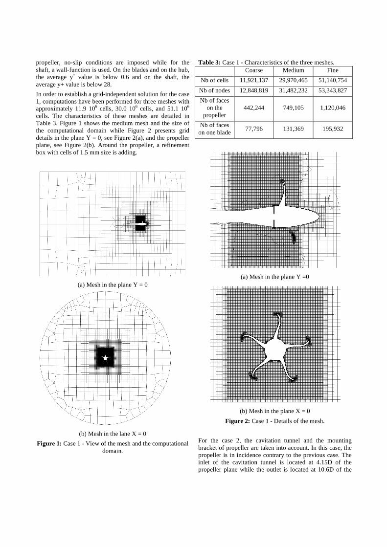
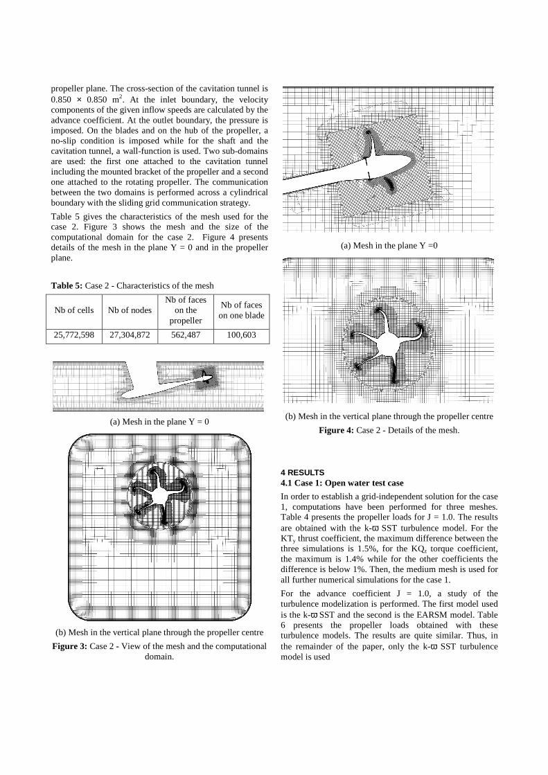
In order to establish a grid-independent solution for the case 1, computations have been performed for three meshes with approximately 11.9 106 cells, 30.0 106 cells, and 51.1 106 cells. The characteristics of these meshes are detailed in Table 3. Figure 1 shows the medium mesh and the size of the computational domain while Figure 2 presents grid details in the plane Y = 0, see Figure 2(a), and the propeller plane, see Figure 2(b). Around the propeller, a refinement box with cells of 1.5 mm size is adding.

(a) Mesh in the plane Y = 0

(b) Mesh in the lane X = 0

Figure 1: Case 1 - View of the mesh and the computational domain.

Table 3: Case 1 - Characteristics of the three meshes. Coarse Medium Fine

Nb of cells 11,921,137 29,970,465 51,140,754

Nb of nodes 12,848,819 31,482,232 53,343,827

Nb of faces on the

propeller 442,244 749,105 1,120,046

Nb of faces on one blade

77,796 131,369 195,932

(a) Mesh in the plane Y =0

(b) Mesh in the plane X = 0

Figure 2: Case 1 - Details of the mesh.

For the case 2, the cavitation tunnel and the mounting bracket of propeller are taken into account. In this case, the propeller is in incidence contrary to the previous case. The inlet of the cavitation tunnel is located at 4.15D of the propeller plane while the outlet is located at 10.6D of the

propeller plane. The cross-section of the cavitation tunnel is 0.850 × 0.850 m2. At the inlet boundary, the velocity components of the given inflow speeds are calculated by the advance coefficient. At the outlet boundary, the pressure is imposed. On the blades and on the hub of the propeller, a no-slip condition is imposed while for the shaft and the cavitation tunnel, a wall-function is used. Two sub-domains are used: the first one attached to the cavitation tunnel including the mounted bracket of the propeller and a second one attached to the rotating propeller. The communication between the two domains is performed across a cylindrical boundary with the sliding grid communication strategy.

Table 5 gives the characteristics of the mesh used for the case 2. Figure 3 shows the mesh and the size of the computational domain for the case 2. Figure 4 presents details of the mesh in the plane Y = 0 and in the propeller plane.

Table 5: Case 2 - Characteristics of the mesh

Nb of cells Nb of nodes Nb of faces

on the propeller

Nb of faces on one blade

25,772,598 27,304,872 562,487 100,603

(a) Mesh in the plane Y = 0

(b) Mesh in the vertical plane through the propeller centre

Figure 3: Case 2 - View of the mesh and the computational domain.

(a) Mesh in the plane Y =0

(b) Mesh in the vertical plane through the propeller centre

Figure 4: Case 2 - Details of the mesh.

4 RESULTS 4.1 Case 1: Open water test case

In order to establish a grid-independent solution for the case 1, computations have been performed for three meshes. Table 4 presents the propeller loads for J = 1.0. The results are obtained with the k-ω SST turbulence model. For the KTy thrust coefficient, the maximum difference between the three simulations is 1.5%, for the KQz torque coefficient, the maximum is 1.4% while for the other coefficients the difference is below 1%. Then, the medium mesh is used for all further numerical simulations for the case 1.

For the advance coefficient J = 1.0, a study of the turbulence modelization is performed. The first model used is the k-ω SST and the second is the EARSM model. Table 6 presents the propeller loads obtained with these turbulence models. The results are quite similar. Thus, in the remainder of the paper, only the k-ω SST turbulence model is used

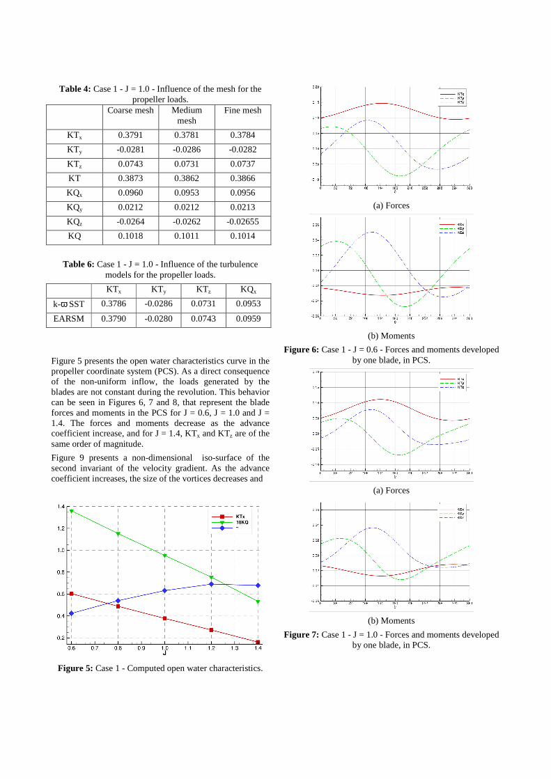
Table 4: Case 1 - J = 1.0 - Influence of the mesh for the propeller loads.

Coarse mesh Medium mesh

Fine mesh

KTx 0.3791 0.3781 0.3784

KTy -0.0281 -0.0286 -0.0282

KTz 0.0743 0.0731 0.0737

KT 0.3873 0.3862 0.3866

KQx 0.0960 0.0953 0.0956

KQy 0.0212 0.0212 0.0213

KQz -0.0264 -0.0262 -0.02655

KQ 0.1018 0.1011 0.1014

Table 6: Case 1 - J = 1.0 - Influence of the turbulence models for the propeller loads.

KTx KTy KTz KQx

k-ω SST 0.3786 -0.0286 0.0731 0.0953

EARSM 0.3790 -0.0280 0.0743 0.0959

Figure 5 presents the open water characteristics curve in the propeller coordinate system (PCS). As a direct consequence of the non-uniform inflow, the loads generated by the blades are not constant during the revolution. This behavior can be seen in Figures 6, 7 and 8, that represent the blade forces and moments in the PCS for J = 0.6, J = 1.0 and J = 1.4. The forces and moments decrease as the advance coefficient increase, and for J = 1.4, KTx and KTz are of the same order of magnitude.

Figure 9 presents a non-dimensional iso-surface of the second invariant of the velocity gradient. As the advance coefficient increases, the size of the vortices decreases and

Figure 5: Case 1 - Computed open water characteristics.

(a) Forces

(b) Moments

Figure 6: Case 1 - J = 0.6 - Forces and moments developed by one blade, in PCS.

(a) Forces

(b) Moments


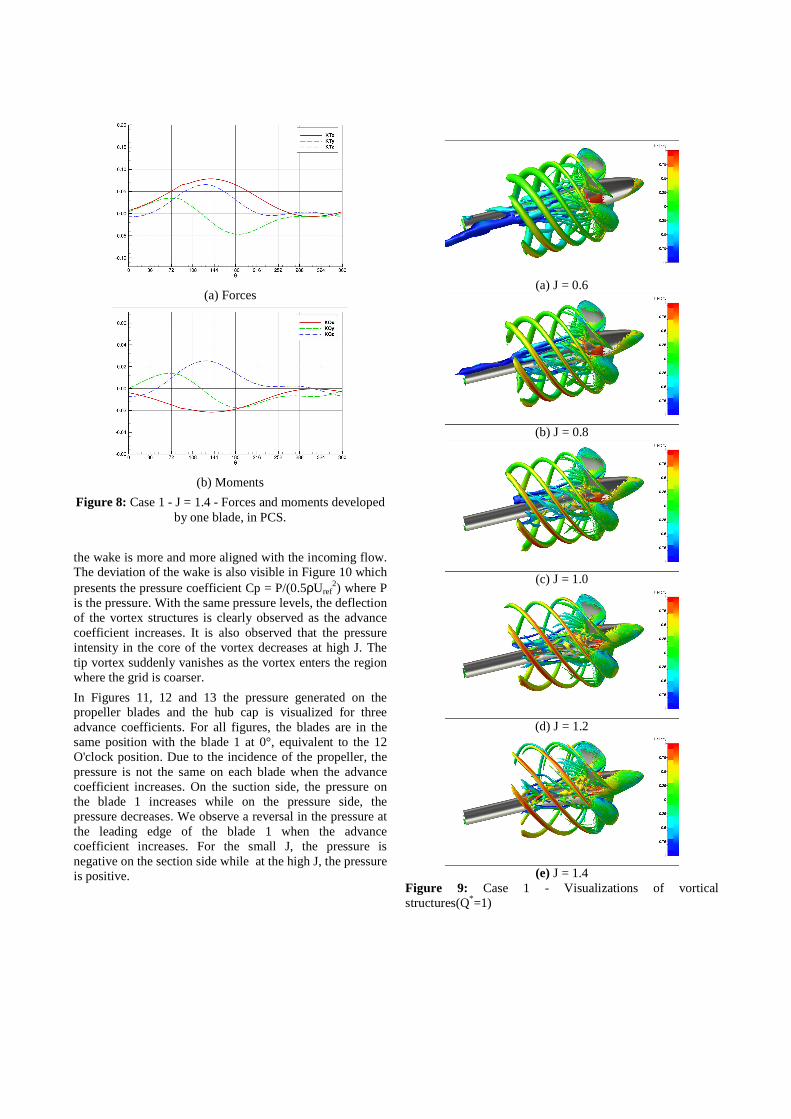
(a) Forces

(b) Moments


the wake is more and more aligned with the incoming flow. The deviation of the wake is also visible in Figure 10 which presents the pressure coefficient Cp = P/(0.5ρUref

2) where P is the pressure. With the same pressure levels, the deflection of the vortex structures is clearly observed as the advance coefficient increases. It is also observed that the pressure intensity in the core of the vortex decreases at high J. The tip vortex suddenly vanishes as the vortex enters the region where the grid is coarser.

In Figures 11, 12 and 13 the pressure generated on the propeller blades and the hub cap is visualized for three advance coefficients. For all figures, the blades are in the same position with the blade 1 at 0°, equivalent to the 12 O'clock position. Due to the incidence of the propeller, the pressure is not the same on each blade when the advance coefficient increases. On the suction side, the pressure on the blade 1 increases while on the pressure side, the pressure decreases. We observe a reversal in the pressure at the leading edge of the blade 1 when the advance coefficient increases. For the small J, the pressure is negative on the section side while at the high J, the pressure is positive.

(a) J = 0.6

(b) J = 0.8

(c) J = 1.0

(d) J = 1.2

(e) J = 1.4

Figure 9: Case 1 - Visualizations of vortical structures(Q*=1)

(a) J = 0.6

(b) J = 0.8

(c) J = 1.0

(d) J = 1.2

(e) J = 1.4

Figure 10: Case 1 - Pressure in the plane Y = 0.

(a) Suction side

(b) Pressure side

Figure 11: Case 1 - J = 0.6 - Pressure fields on propeller blades.

(a) Suction side

(b) Pressure side

Figure 12: Case 1 - J = 1-0 - Pressure fields on propeller blades.

(a) Suction side

(b) Pressure side

Figure 13: Case 1 - J = 1.4 - Pressure fields on propeller blades.

4.2 Case 2: Cavitation test case

For all the simulations, the Sauer model is used to predict the cavitation.

In order to evaluate the influence of the cavitating behavior on the propeller performance, we compare the results of the non-cavitating and cavitating flow at three advance coefficients. In Table 7, the predicted values of the thrust and torque coefficients, for the non-cavitating and cavitating flow regimes, are collected. For all the operational conditions, cavitation affects the propeller thrust negatively.

Table 7: Case 2 - Thrust and torque coefficients in PCS.

J = 1.019 J = 1.269 J = 1.408 Forces &

Torque No cav

σ = 2.024

No cav

σ = 1.424

No cav

σ = 2.000

KTx 0.4021 0.3527 0.2663 0.1220 0.1825 0.0838

KTy -0.044 -0.026 -0.058 -0.032 -0.066 -0.037

KTz 0.0835 0.0786 0.1158 0.0590 0.1393 0.0995

KQ 0.1005 0.0903 0.0487 0.0484 0.0581 0.0443

(a) Without cavitation

(b) With cavitation

Figure 14: Case 2-1 - Visualizations of vortical structures (Q*=1)


(b) With cavitation



(b) With cavitation


Figures 14, 15 and 16 show the vortical structures for the three advance coefficients with and without cavitation. For all cases, we observe the vortex generated by the tip vortices. As for the case of open water, these vortices disappear when the mesh is not fine enough.

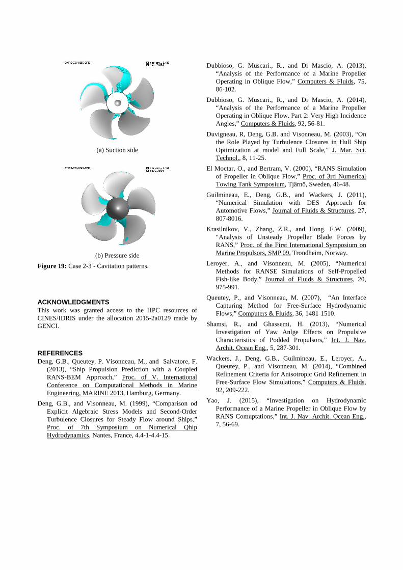
Figures 17, 18 and 19 show cavity patterns on the blades for each test case. With these figures, we observe that the cavity patterns are only located on the blades while with he previous figures, we note that the vortices going to the wake of the propeller have not vapor fraction inside. Then it is not clear to concluded that this damping of the vapor fraction is due to the turbulence modeling and/or the cavitation model itself.

5 CONCLUSIONS AND FUTURE WORK In this paper, the cavitating performance and open water performance of the PPTC model at an incidence was numerically simulated using the ISIS-CFD flow solver. The turbulence is modeled with the k-ω SST model and the cavitation with the Sauer model. Simulations were carried out following the recommendations of the SMP'15 Workshop. The requested thrust and torque coefficient are presented for open water case. The cavity surface on the propeller is presented for the cavitating cases.

(a) Suction side

(b) Pressure side

Figure 17: Case 2-1 - Cavitation patterns.

(a) Suction side

(b) Pressure side


(a) Suction side

(b) Pressure side


ACKNOWLEDGMENTS This work was granted access to the HPC resources of CINES/IDRIS under the allocation 2015-2a0129 made by GENCI.

REFERENCES Deng, G.B., Queutey, P. Visonneau, M., and Salvatore, F.

(2013), “Ship Propulsion Prediction with a Coupled RANS-BEM Approach,” Proc. of V. International Conference on Computational Methods in Marine Engineering, MARINE 2013, Hamburg, Germany.

Deng, G.B., and Visonneau, M. (1999), “Comparison od Explicit Algebraic Stress Models and Second-Order Turbulence Closures for Steady Flow around Ships,” Proc. of 7th Symposium on Numerical Qhip Hydrodynamics, Nantes, France, 4.4-1-4.4-15.

Dubbioso, G. Muscari., R., and Di Mascio, A. (2013), “Analysis of the Performance of a Marine Propeller Operating in Oblique Flow,” Computers & Fluids, 75, 86-102.

Dubbioso, G. Muscari., R., and Di Mascio, A. (2014), “Analysis of the Performance of a Marine Propeller Operating in Oblique Flow. Part 2: Very High Incidence Angles,” Computers & Fluids, 92, 56-81.

Duvigneau, R, Deng, G.B. and Visonneau, M. (2003), “On the Role Played by Turbulence Closures in Hull Ship Optimization at model and Full Scale,” J. Mar. Sci. Technol., 8, 11-25.

El Moctar, O., and Bertram, V. (2000), “RANS Simulation of Propeller in Oblique Flow,” Proc. of 3rd Numerical Towing Tank Symposium, Tjärnö, Sweden, 46-48.

Guilmineau, E., Deng, G.B., and Wackers, J. (2011), “Numerical Simulation with DES Approach for Automotive Flows,” Journal of Fluids & Structures, 27, 807-8016.

Krasilnikov, V., Zhang, Z.R., and Hong. F.W. (2009), “Analysis of Unsteady Propeller Blade Forces by RANS,” Proc. of the First International Symposium on Marine Propulsors, SMP'09, Trondheim, Norway.

Leroyer, A., and Visonneau, M. (2005), “Numerical Methods for RANSE Simulations of Self-Propelled Fish-like Body,” Journal of Fluids & Structures, 20, 975-991.

Queutey, P., and Visonneau, M. (2007), “An Interface Capturing Method for Free-Surface Hydrodynamic Flows,” Computers & Fluids, 36, 1481-1510.

Shamsi, R., and Ghassemi, H. (2013), “Numerical Investigation of Yaw Anlge Effects on Propulsive Characteristics of Podded Propulsors,” Int. J. Nav. Archit. Ocean Eng., 5, 287-301.

Wackers, J., Deng, G.B., Guilmineau, E., Leroyer, A., Queutey, P., and Visonneau, M. (2014), “Combined Refinement Criteria for Anisotropic Grid Refinement in Free-Surface Flow Simulations,” Computers & Fluids, 92, 209-222.

Yao, J. (2015), “Investigation on Hydrodynamic Performance of a Marine Propeller in Oblique Flow by RANS Comuptations,” Int. J. Nav. Archit. Ocean Eng., 7, 56-69.

Documents

Numerical Simulations of the ... - NUMECA International