(SYA) 15-1

Numerical Simulation of Vortex Flows Around Missile Configurations

P. Champigny, P. d’EspineyONERA, 29, avenue de la Division Leclerc

B.P. 72, 92322 Chatillon, Cedex, France

M. Brédif, H. BroussardMATRA BAe Dynamics37, avenue Louis Breguet

Boîte postale 178146 Velizy-Villacoublay Cedex

France

J.-P. Gillybœuf, Y. KergaravatEADS Aerospatiale Matra Missiles

Dept. E/SCG/N2-18 rue Beranger92320 Chatillon

France

SUMMARY

This paper describes the work achieved during the recent yearsto improve the quality of Navier-Stokes computations forindustrial purpose. The main axes for improvement are thegrid adaptation strategy, the turbulence modeling and theapplication to industrial missiles. A few years ago, Navier-Stokes computations were rarely run for externalaerodynamics simulations. This is no longer true. Bothindustrial companies (EADS Aerospatiale Matra Missiles andMATRA BAe Dynamics France) now use it on a regular basis.Nevertheless some progresses are still necessary, especiallyfor the prediction of the axial force.

1. INTRODUCTION

The accurate prediction of missile aerodynamic characteristicsis a major task for the missile industry. It can rely on Eulercomputations only to a certain extent, depending on Machnumber and angle of attack values. This approach has beenwidely used up to now. Nevertheless, Euler computations cannot be used for all cases nor all characteristics. For examplethey are unable to accurately predict the axial force or therolling moment coefficients. For this reason, a collaborationbetween ONERA and the French missile manufacturers EADS

Aerospatiale Matra Missiles and MATRA BAe Dynamics Francehas been undertaken in order to assess Navier-Stokessimulations for missile external aerodynamics. In order toachieve this goal, the common study – hereafter called SIAM –has been divided into three parts.

The first part of the work is dedicated to grid adaptation inviscous regions. Two independent tools have been developedand validated. With the first tool, a multidomain mesh can bemodified or refined in the boundary layers, remainingcontinuous between two domains. The second tool generates anew grid for each wake or vortex that has been detected in aflow. The new meshes overlap the initial one and the

communication between all of them is achieved with thechimera technique.

In the second part of the work, the turbulence modeling hasbeen handled with care. The number of turbulence modelsavailable in the literature is tremendous. Two categories havebeen retained (algebraic models and transport equationmodels) and one model has been selected for each category(Baldwin-Lomax and Spalart-Allmaras). An accurate androbust formulation of each model has been derived. Someexamples related to generic configurations demonstrate themerits of these choices.

In the third part of the work, one turbulence model and onegrid adaptation tool have been applied to industrial missiles.

The three components of the work have been separated onlybecause it makes the presentation clearer but in fact they areclosely combined. They are described in the next sections.

For all the configurations presented, the numerical solutionswere obtained with the AEROLOG code developed by MATRA

BAe Dynamics France [3] and with the FLU3M code developedat ONERA [1] in collaboration with EADS Aerospatiale MatraMissiles. The grids were built according to the general rulesthat have been found during the work to get grid independentsolutions. The computations have been carried out with thewind tunnel conditions. The aerodynamic coefficients arealways calculated in the missile reference frame.

The following notations are used:

CA axial force coefficient (pressure and skinfriction),

Cl rolling moment coefficient,

CN normal force coefficient,

Cp pressure coefficient,

D missile diameter,

Paper presented at the RTO AVT Symposium on “Advanced Flow Management: Part A – Vortex Flows andHigh Angle of Attack for Military Vehicles”, held in Loen, Norway, 7-11 May 2001, and published in RTO-MP-069(I).

Report Documentation Page Form ApprovedOMB No. 0704-0188

Public reporting burden for the collection of information is estimated to average 1 hour per response, including the time for reviewing instructions, searching existing data sources, gathering andmaintaining the data needed, and completing and reviewing the collection of information. Send comments regarding this burden estimate or any other aspect of this collection of information,including suggestions for reducing this burden, to Washington Headquarters Services, Directorate for Information Operations and Reports, 1215 Jefferson Davis Highway, Suite 1204, ArlingtonVA 22202-4302. Respondents should be aware that notwithstanding any other provision of law, no person shall be subject to a penalty for failing to comply with a collection of information if itdoes not display a currently valid OMB control number.

1. REPORT DATE 00 MAR 2003

2. REPORT TYPE N/A

3. DATES COVERED -

4. TITLE AND SUBTITLE Numerical Simulation of Vortex Flows Around Missile Configurations

5a. CONTRACT NUMBER

5b. GRANT NUMBER

5c. PROGRAM ELEMENT NUMBER

6. AUTHOR(S) 5d. PROJECT NUMBER

5e. TASK NUMBER

5f. WORK UNIT NUMBER

7. PERFORMING ORGANIZATION NAME(S) AND ADDRESS(ES) NATO Research and Technology OrganisationBP 25, 7 Rue Ancelle,F-92201 Neuilly-Sue-Seine Cedex, France

8. PERFORMING ORGANIZATIONREPORT NUMBER

9. SPONSORING/MONITORING AGENCY NAME(S) AND ADDRESS(ES) 10. SPONSOR/MONITOR’S ACRONYM(S)

11. SPONSOR/MONITOR’S REPORT NUMBER(S)

12. DISTRIBUTION/AVAILABILITY STATEMENT Approved for public release, distribution unlimited

13. SUPPLEMENTARY NOTES Also see: ADM001490, Presented at RTO Applied Vehicle Technology Panel (AVT) Symposium heldinLeon, Norway on 7-11 May 2001, The original document contains color images.

14. ABSTRACT

15. SUBJECT TERMS

16. SECURITY CLASSIFICATION OF: 17. LIMITATION OF ABSTRACT

UU

18. NUMBEROF PAGES

14

19a. NAME OFRESPONSIBLE PERSON

a. REPORT unclassified

b. ABSTRACT unclassified

c. THIS PAGE unclassified

Standard Form 298 (Rev. 8-98) Prescribed by ANSI Std Z39-18

(SYA) 15-2

XCP/D position of the center of pressure from the nose,

α angle of attack,

β sideslip angle,

φ roll angle or circumferential angle.

2. MESH ADAPTATION

2.1. Introduction

Boundary layer separations, wakes and vortices are some ofthe viscous phenomena that occur around missiles. It isnecessary to represent them accurately because they are ofhigh importance for many missile aerodynamic characteristics.For example the axial force coefficient is linked to theboundary layer thickness; the aerodynamic characteristics of alifting surface can be strongly affected if the surface is locatedwithin a wake or a vortex.

The accuracy of a numerical solution depends on thenumerical scheme and the turbulence model, and also on thegrid quality. The second point is considered here. Let ussuppose that an initial multidomain conform mesh is available.

The boundary layers are defined through topological data (forexample the wall boundary conditions) and physical data (forexample the Reynolds number). The mesh is then modified orrefined in the boundary layers with a tool named AMCOLI.AMCOLI does not require the initial flow in addition to theinitial grid.

Grid adaptation in wakes and vortices is based on a differentapproach. The wakes and the vortices are partly describedthrough topological and physical data and then they aredetected in the initial flow with a tool named AMSITO.Moreover AMSITO does not modify the initial mesh butgenerates an overlapping grid for each wake and each vortexthat has been detected. The new meshes and the initial one arenot continuous and it is necessary to use the chimera techniquein order to accomplish the communication between all ofthem.

The grid adaptation strategy is presented on figure 1.

Adaptation inwakes and vortices

Adaptation inboundary layers

Euler mesh

Eulercomputation

AMCOLI

NS computation

AMSITO

NS computation

Figure 1 – Grid adaptation strategy

AMCOLI and AMSITO have been developed and validated withvarious configurations. They are completely independent ofthe CFD codes. In the next two paragraphs, their principle isexposed and some applications are presented.

2.2. Grid adaptation in boundary layers

The grid adaptation tool AMCOLI can be applied to transforman Euler mesh into a Navier-Stokes one, or to modify aNavier-Stokes grid according to new flow conditions. It alsobuilds a flow in the boundary layers of the adapted mesh;outside the boundary layers, the initial flow is maintained ifavailable otherwise the flow is uniform. AMCOLI gives someinformation to check the new mesh (smoothness, accuracynear the walls, …).

Compared to a classical grid generation tool, AMCOLI has thefollowing advantages:

• the time required to create a Navier-Stokes mesh ismuch lower since the tool carries out many of theoperations that are traditionally done by the user,

• the quality of the grid is improved by the use of thephysical characteristics of the boundary layers,

• the construction of a flow in the adapted meshshould attenuate the convergence problems andaccelerate the convergence itself.

AMCOLI requires the following data:

• the initial mesh (with or without the correspondingflow),

• some data which describe the gas and the flow(Prandtl number, Mach number, …),

• the grid points and grid lines which represent thebeginning of the boundary layers,

• the description of the adaptation in the boundary

layers (number of points, +y for the first cell, law

for the distribution of points).

AMCOLI computes the main characteristics of the boundarylayers (thickness, wall skin friction coefficient, …) withsemi-empirical formulas. It works for very complicatedtopologies. It can handle axis singularities, C type and O typedecompositions. The mesh adaptation applied in a domain isautomatically extended to the adjacent domains, in alltopological directions. The grid is modified only in thetopological directions that are normal to a wall.

AMCOLI has been validated with various conventional andindustrial configurations. Only one of them is presented as anillustration. An Euler mesh is built around a missile with aclassical grid generation tool (figure 2). It contains 1 130 000points. There are C-O type domains around the wings and thefins.

(SYA) 15-3

Figure 2 – Euler mesh around a missile

All the boundary layers are taken into account (over thefuselage, the four wings and the four fins). The Navier-Stokesmesh is obtained with AMCOLI after 17 minutes on oneprocessor of a SGI Origin 2000. It contains 3 930 000 pointsand is smooth (figure 3).

Figure 3 – Comparison between the initial Euler mesh and theNavier-Stokes mesh obtained with AMCOLI

After the validation of the tool, it was interesting to try todefine some general rules which ensure that the numericalsolution obtained on an adapted mesh does not depend on thegrid adaptation parameters. For this reason, various parametricstudies have been carried out on different configurations withthe Baldwin-Lomax and the Spalart-Allmaras turbulencemodels (see §3). The conclusions, common to the differentcases, can be summarized as follow:

• the law for the distribution of points (bigeometric orhyperbolic tangent) does not affect the solution,

• the boundary layers should contain at least 30 points,

• for the first cell, +y should be less than 3.

2.3. Grid adaptation in wakes and vortices

The grid adaptation tool AMSITO is able to detect wakes andvortices in a numerical flow and generates a new mesh foreach of them. It also computes the flow in the new grids andgives some information to control what has been done.

AMSITO requires the following data:

• the initial mesh with the corresponding flow,

• the grid lines which represent the beginning of thewakes,

• some criteria to find the vortices and to follow theprescribed wakes,

• the description of the mesh adaptation (number ofpoints, …).

From the grid line located at the trailing edge of a liftingsurface, AMSITO builds a surface that represents the wake core(figures 4 and 5).

Figure 4 – Flow around a conventional missile

Figure 5 – Representation of the core of the wakes

This surface is then used to build two others, which representthe wake shape, and from which the overlapping mesh iscreated (figures 6 and 7).

Figure 6 – Representation of the shape of a wake

(SYA) 15-4

Figure 7 – Overlapping grid for a wake

The principle is similar for the vortices, except that theirbeginning is not prescribed by the user but automaticallydetected in the flow (figure 8).

Figure 8 – Flow around a conventional missile

Then AMSITO generates for each vortex a line for the core, asurface that includes the vortex and finally the overlappinggrid itself (figures 9 to 11).

Figure 9 – Representation of the core of the vortices

Figure 10 – Representation of the shape of the vortices

Figure 11 – Overlapping grids for the vortices

The detection of the physical structures in the flow (the coreand the shape of the wakes and the vortices) is based on acombination of simple criteria (for example local minimumfor the total pressure, local maximum for the rotational,absolute value of the helicity greater than 0.9, …). The criteriaare defined by the user and the wakes and the vortices areautomatically tracked.

The overlapping grids created by AMSITO do not match theoriginal one. Thus it is necessary to use the chimera techniquefor the communication between all the meshes.

AMSITO has been validated with various configurations. Twoexamples concerning conventional missiles have beenpresented above. The initial meshes contain 2 075 700 points(wakes) and 2 552 500 points (vortices). The overlappinggrids are obtained after 10 minutes on one processor of a SGIOrigin 2000.

An additional analysis is in progress with the intention offinding some general conditions which guarantee that thenumerical solution obtained on an adapted mesh isindependent of the grid adaptation parameters. The followingparameters are examined:

• the number of points in an overlapping grid in thestreamwise direction of a wake or a vortex,

• the number of points in the two transversaldirections,

• the size of an overlapping grid (is it necessary tooverlap the whole wake or vortex ?),

• the size and the position of the region where theinitial and the overlapping meshes communicatewith each other.

(SYA) 15-5

2.4. Conclusion

Two grid adaptation tools have been developed and validated.They are independent of the CFD codes. The tool for theboundary layers is now widely used for industrial applications.The criteria for an accurate and mesh independent solution areknown. The tool for wakes and vortices works but it is stillinvestigated to find general and suitable utilization rules.

The accuracy of a numerical solution does not depend only onthe grid quality. For this reason, the turbulence modeling mustbe handled with care.

3. TURBULENCE MODELING

As mentioned previously, two turbulence models have beenmainly used for this study. They are the well-known Baldwin-Lomax model and the Spalart-Allmaras model (one transportequation). These models are considered as offering a goodcompromise between accuracy and computational cost forindustrial applications.

3.1. Baldwin-Lomax model

This algebraic turbulence model represents a usual choice forexternal aerodynamics applications because of its minimalextra CPU cost and memory requirements. The estimate of theturbulent viscosity is based on a length scale, related to themaximum of the well-known Baldwin F function. In order toavoid an over-estimate of the turbulent viscosity when theflow separates (or in the vicinity of vortices), twomodifications have been implemented: a cut-off distance forthe search of the maximum of F and the well-knownprocedure of Degani and Schiff [2]. The model works even ifthere is more than one wall.

3.2. Spalart-Allmaras model

To overcome limitations of algebraic models, an eddyviscosity transport equation model has been implemented [4].Baldwin and Barth recently rediscovered this class of one-equation models, proposed originally by Nee and Kovasznayinin the sixties. The Spalart-Allmaras model has been chosendue to the satisfactory results obtained over a wide range offlows and due to its numerical properties. In this model a stepby step procedure is used to develop the transport equation forflows with increasing complexity. Moreover this one-equationmodel naturally takes history effects into account.

4. SIMULATION OF VORTEX FLOWS AROUNDGENERIC CONFIGURATIONS

4.1. Ogive-cylinder configuration

The first test case consists of a very simple circular body (3Dogive + cylinder) at M = 2 and α = 10° [2] (figure 12). Themissile length is 16 D. This configuration has been chosenbecause it represents a very simple vortical flow, which isconvenient to compare different turbulence models. Moreoverdetailed experimental results and various computationalresults (Euler, laminar, k-ε) are available. Two grids, namedg0 and g1, are used. The only difference is that the number ofpoints on the circumference in grid g0 is half the number in

grid g1. One Baldwin-Lomax + cut-off, two Baldwin-Lomax + Degani-Schiff and one Spalart-Allmarascomputations have been performed.

Figure 12 – Ogive-cylinder – Total pressure contours atM = 2, α = 10°

Figure 13 shows that the vortical structure is globally correct.However the solutions obtained with the Baldwin-Lomaxmodel can be very different (see the pressure distribution,figure 14), according to the variant used (Baldwin-Lomax +cut-off or Baldwin-Lomax + Degani-Schiff). Nevertheless theresults are very close between Baldwin-Lomax + Degani-Schiff, Spalart-Allmaras and k-ε for the vortices, as well as forthe local and global forces (figure 15). This last figure alsoshows the importance of taking the viscous effects(comparison with the Euler solution) and the turbulence(comparison with the laminar solution) into account.

Figure 13 – Ogive-cylinder – Total pressure contours atM = 2, α = 10°, X/D = 7

(SYA) 15-6

Figure 14 – Ogive-cylinder – Pressure distribution atM = 2, α = 10°, X/D = 7

Figure 15 – Ogive-cylinder – Normal force coefficient atM = 2, α = 10°

4.2.Body-fin configuration

The second test case is a body-fin missile at M = 2 andφ = 22.5° (non-symmetric roll angle). The forebody vorticesact on the fins (figure 16). They can modify the aerodynamiccharacteristics of the missile. In particular they create aninduced rolling moment. For this reason it is interesting tostudy this configuration. Euler and Spalart-Allmarascomputations have been carried out with the same grid, whichcontains around 1 000 000 points. The missile length is 16 D.

Figure 16 – Body-fin – Spalart-Allmaras solution atM = 2, α = 11.4°, φ = 22.5°

The prediction of the normal force (figure 17) and the positionof the center of pressure (figure 18) is very good for theSpalart-Allmaras computations, and surprisingly not so badfor the Euler ones. This can be explained by the fact that in theEuler solutions the body normal force is underestimated (see§4.1), whereas the fins normal force is overestimated (no orsmaller effect of the vortices).

The situation is not the same for the rolling moment (figure19). The discrepancies with the experimental results are verysmall for the Spalart-Allmaras results and much higher for theEuler results. This shows that the accurate prediction of therolling moment requires the modeling of the viscous effects. Itis not surprising since the rolling moment is highly dependenton the individual contribution of each fin.

Figure 17 – Body-fin – Normal force coefficient at M = 2,φ = 22.5°

(SYA) 15-7

Figure 18 – Body-fin – Position of the center of pressure atM = 2, φ = 22.5°

Figure 19 – Body-fin – Rolling moment coefficient atM = 2, φ = 22.5°

It is interesting to continue the analysis with the axial forcecoefficient. The difference between the Spalart-Allmaras andthe experimental results is about 6%. As an indication, thediscrepancy is almost zero for M = 3 and M = 4.5.

CAM = 2α = 0°

M = 3α = 0°

M = 4.5α = 0°

Experiment 0.307 0.263 0.23

Spalart-Allmaras model0.32

(+6%)0.265

(< 1%)0.231

(< 1%)

4.3. Canard-body-fin configuration

The last test case is a canard-body-fin missile at M = 2 andφ = 45°. It represents a more realistic configuration sincedifferent kinds of vortices act on the fins (figure 20). Euler andBaldwin-Lomax + cut-off computations have been run withthe same grid, which contains around 4 million points. Themissile length is 16 D.

Figure 20 – Canard-body-fin configuration –Total pressurecontours at M = 2, α = 10°, φ = 45°

Figure 21 shows the complex vortical structure, for a sectionbetween the canards and the tail fins. Again, only a Navier-Stokes (Baldwin-Lomax) solution can give a detailed andrepresentative description of this vortical structure.Nevertheless, in the Euler solution some vortices are present,those coming from the wake of the forward canards.

a – Experiment

b – Euler (left) and Navier-Stokes (right) solutions

Figure 21 – Canard-body-fin – Total pressure contours atM = 2, α = 10°, φ = 45°, X/D = 10

The normal force coefficient and the position of the center ofpressure are well predicted by both the Euler and the Navier-Stokes computations (figures 22 and 23). Is it the same for theloads on the fins ? In fact these loads are strongly affected bythe vortices acting on the fins. For this reason the Eulercomputations should give bad quality results, which is

(SYA) 15-8

confirmed on figure 24. On the contrary, the Baldwin-Lomaxresults are very accurate.

0

1

2

3

4

5

6

7

8

0 2 4 6 8 10 12 14 16 18 Alpha

CN

expe

Euler

NS-BL

Figure 22 – Canard-body-fin – Normal force coefficient atM = 2, φ = 45°

6,00

6,50

7,00

7,50

8,00

0 2 4 6 8 10 12 14 16 18 Alpha

Xcp/D

expe

Euler

NS-BL

Figure 23 – Canard-body-fin – Position of the center ofpressure at M = 2, φ = 45°

CN upper fin

0

0,1

0,2

0,3

0,4

0,5

0 2 4 6 8 10 12 14 16 Alpha

Expe

NS-BL

Euler

Figure 24 – Canard-body-fin – Fin normal force atM = 2, φ = 45°

4.4. Conclusions

Generic configurations have been studied for supersonic flowsand various angles of attack.

For the ogive-cylinder configuration, a detailed study has beenperformed at α = 10°. The normal force coefficient induced bythe vortical flow which develops on the leeward side is verysensitive to the viscous effects and to the turbulence model.None of the models is completely satisfactory: the Baldwin-Lomax model needs specific handling of the cut-off parameterwhereas the Spalart-Allmaras and k-ε (Jones-Launder) modelslead to results that are very close one to the other butoverestimate the turbulent viscosity.

Taking the vortical flow into account is also important topredict the rolling moment on configurations with rear fins.For both the Baldwin-Lomax and the Spalart-Allmaras modelsa good estimate of this coefficient has been obtained. Howeverthe vortical flow has no visible effect on global longitudinalcharacteristics (CN and XCP/D). This is shown by the goodprediction obtained with Euler calculations.

5. SIMULATION OF COMPLEX FLOWS AROUNDINDUSTRIAL CONFIGURATIONS

The aim is to evaluate the improvement in the prediction andthe quality of the results on configurations which arerepresentative of two main families of missiles:

• the cruciform supersonic missiles,

• the stealth subsonic cruise missiles.

It has been interesting to assess the generality, the robustnessand user-friendliness of the new developed tools. All theNavier-Stokes computations have been carried out with theBaldwin-Lomax + cut-off model.

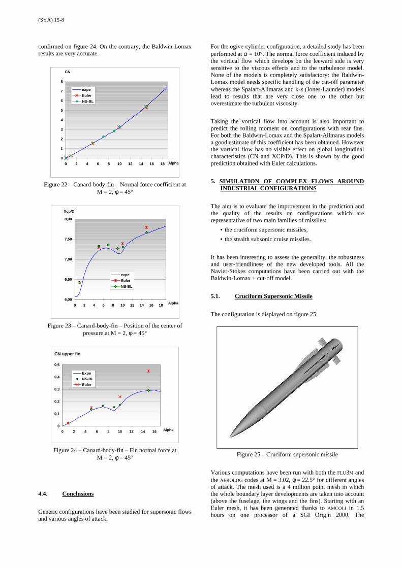
5.1. Cruciform Supersonic Missile

The configuration is displayed on figure 25.

Figure 25 – Cruciform supersonic missile

Various computations have been run with both the FLU3M andthe AEROLOG codes at M = 3.02, φ = 22.5° for different anglesof attack. The mesh used is a 4 million point mesh in whichthe whole boundary layer developments are taken into account(above the fuselage, the wings and the fins). Starting with anEuler mesh, it has been generated thanks to AMCOLI in 1.5hours on one processor of a SGI Origin 2000. The

(SYA) 15-9

computational time needed to get the result for one angle ofattack is about 180 hours on the same machine.

Global aerodynamic loads depending on the angle of attackare displayed on figure 26 for the normal force coefficient, onfigure 27 for the rolling moment, and on figure 28 for theposition of the center of pressure. The numerical results are ingood agreement with the experimental data. The maximaldiscrepancy on the prediction of the normal force coefficient isabout 3%. For the prediction of the position of the center ofpressure, the accuracy is about 0.1 D.

The prediction of the rolling moment coefficient, though lessaccurate than for the normal force coefficient, is correct. Theglobal curve shape is well predicted. Values are in fairagreement with experiments, except for the angles of attackaround 10°.

ExperimentalAEROLOGFLU3M

CN

Figure 26 – Cruciform supersonic missile – Normal forcecoefficient at M = 3.02, φ = 22.5°

ExperimentalAEROLOGFLU3M

Cl

Figure 27 – Cruciform supersonic missile – Rolling momentcoefficient at M = 3.02, φ = 22.5°

0.6 D

Figure 28 – Cruciform supersonic missile – Position of thecenter of pressure at M = 3.02, φ = 22.5°

The discrepancies in results obtained before this study aredisplayed in terms of rolling moment coefficient in the arraybelow. One can see the improvement of the prediction of therolling moment coefficient: the Euler computations wereleading to an average discrepancy of 94%, whereas theNavier-Stokes results were accurate at an average rate of 39%.Considering the new results, the difference between theexperimental data and the numerical results is includedbetween 0 and 24%. This improvement in the prediction of therolling moment coefficient may be due to the use of a differentmesh (finer O type mesh created according to the general rulesobtained in §2.2, each lifting surface being considered asviscous), to the modification of the Baldwin-Lomax modelformulation, and also to the use of a different numericalscheme.

Discrepancy ofthe prediction

Euler computations 94%

Navier-Stokes computations(before this study – SIAM)

39%

Navier-Stokes computations(after this study – SIAM)

0 to 24%

One problem remains concerning the prediction of the axialforce coefficient. As one can see on figure 29 representing theaxial force coefficient prediction for different angles of attack,the prediction is less than 10% accurate, which is not enoughfor industrial purpose.

CA

Figure 29 – Cruciform supersonic missile – Axial forcecoefficient at M = 3.02, φ = 22.5°

(SYA) 15-10

On the figures 30 and 31, the total pressure field is representedin two sections of the flow at α = 9.5° (X/D = 11.6 locatedaround the wings and X/D = 14.5 located at the rear part of themissile). On figure 30, two different phenomena can be seen:there is an interaction between the forebody vortices and thewings on the upper side of the missile. Side vortices are alsodeveloping. The rolling angle of the flow acts on thedevelopment of these vortices. On the lower-right wing, thevortex is spreading since the fuselage hides it. On the lower-left wing, the vortex is thrown onto the fuselage, and thus it isnot spread at all. On the figure 31, the forebody vortices, theside vortices of the wings and the wakes of the wings haveinteracted with the fins. The side vortices of the fins and theirwakes can be seen. The vortex located at the upper-right sideof the missile is less powerful than the one located at theupper-left side. This is due to the fact that the forebody vortexon the left side and the side vortices on the upper-left wingand fin are rotating in the same direction whereas on theupper-right side the vortices are counter-rotating.

AEROLOG

Figure 30 – Cruciform supersonic missile – Total pressurecontours at M = 3.02, α = 9.5°, φ = 22.5°, X/D = 11.6

AEROLOG

Figure 31 – Cruciform supersonic missile – Total pressure contoursat M = 3.02, α = 9.5°, φ = 22.5°, X/D = 14.5

Some other computations have been run with FLU3M. Theycorrespond to a specified angle of attack (α = 15°) anddifferent roll angles for M = 3.02. Global aerodynamic loadsare displayed on figures 32 to 34. The normal forcecoefficient, the rolling moment coefficient and the position ofthe center of pressure are successively displayed.

ExperimentalFLU3M

C N

Figure 32 – Cruciform supersonic missile – Normal forcecoefficient at M = 3.02, α = 15°

ExperimentalFLU3M

C l

Figure 33 – Cruciform supersonic missile – Rolling momentcoefficient at M = 3.02, α = 15°

ExperimentalFLU3M

X C

P / D

0.3 D

Figure 34 – Cruciform supersonic missile – Position of thecenter of pressure at M = 3.02, α = 15°

(SYA) 15-11

Figure 35 – Cruciform supersonic missile – Total pressurecontours at M = 3.02, α = 15°, φ = 60°

The numerical results are in a good agreement with theexperimental data. On the figure 35, the total pressure isdisplayed at φ = 60°. This allows to well understand thecomplexity of the flow through the interaction of the vortices(forebody, side edge) and the wakes with the wings and thefins.

5.2. The Stealth Subsonic Cruise Missile

The configuration looks like the one displayed on figure 36.

Figure 36 – Stealth Subsonic Cruise missile

Various computations have been run with both the FLU3M andthe AEROLOG codes at M = 0.8 and β = 4°, for different anglesof attack. The mesh used is a 4 million point mesh in whichthe whole boundary layer developments are taken into account(above the fuselage and the fins). The computational timeneeded to get the results is about 220 hours on one processorof a SGI Origin 2000. Global aerodynamic loads depending onthe angle of attack are displayed on figure 37 for the normalforce coefficient, on figure 38 for the rolling moment, and onfigure 39 for the position of the center of pressure.

The numerical results are in good agreement with theexperimental data except for high angles of attack (in absolutevalue). The average discrepancy on the prediction of thenormal force coefficient is about 4%. For the prediction of theposition of the center of pressure, the accuracy varies between0 and 0.4 D. Concerning the prediction of the rolling momentcoefficient, the accuracy is about 5%.

Figure 37 – Stealth Subsonic Cruise missile – Normal forcecoefficient at M = 0.8, β = 4°

Figure 38 – Stealth Subsonic Cruise missile – Rolling momentcoefficient at M = 0.8, β = 4°

Figure 39 – Stealth Subsonic Cruise missile – Position of thecenter of pressure at M = 0.8, β = 4°

On the figures 40 and 41, the total pressure is displayed in twosections of the flow at α = –10°. On the first figure, one candistinguish the two forebody vortices and a detached flow onthe middle of the fuselage. On the second figure, there is aninteraction between the forebody vortices and the fins. Theside vortex of the left fin rotates in the same direction as theforebody vortex of this side, whereas both the forebody vortexand side vortex on the right-hand side vanish together.

(SYA) 15-12

Figure 40 – Stealth Subsonic Cruise missile – Total pressurecontours at M = 0.8, α = –10°, β = 4°, X/D = 10

Figure 41 – Stealth Subsonic Cruise missile – Total pressurecontours at M = 0.8, α = –10°, β = 4°, X/D = 15

6. CONCLUDING REMARKS

The meshing tool AMCOLI used to refine Euler grids inside theboundary layer regions is operational and has already beensuccessfully used for industrial applications. It allows savingthe engineer time spent to generate the Navier-Stokes meshes.The boundary layer flow initialization has not yet been usedon industrial configurations even if it has shown some CPUtime saving on generic configurations.

The meshing tool AMSITO used to refine Navier-Stokes meshesinside wakes and vortices regions has been used on genericconfigurations. It still needs to be used on industrialconfigurations.

The Baldwin-Lomax turbulence model has given accurateresults. The prediction of the rolling moment coefficient ismuch more accurate than before. This may also be due to thefact that computations are now run on much finer meshes. Theaxial force coefficient prediction still needs to be improved.

The Spalart-Allmaras model which has been developed andvalidated on generic configurations still needs to be used onindustrial ones. It could be used for more complicatedproblems such as the prediction of the maximal lift of a finbefore stall, the computation of fins with gaps, …

A few years ago, Navier-Stokes computations were rarely runfor external aerodynamics simulations. This is no longer true.Both industrial companies (EADS Aerospatiale Matra Missilesand MATRA BAe Dynamics France) now use it on a regularbasis, thanks to progress made in mesh generation andturbulence modeling, and because they have increased theconfidence in the results.

7. ACKNOWLEDGEMENTS

The SIAM contract (n°98.70.505) has been funded by the DGA

(SPMT) through collaborations between EADS AerospatialeMatra Missiles, MATRA BAe Dynamics France and ONERA.

8. REFERENCES

[1] Ben Khelil S., Guillen P., Lazareff M., Lacau R.-G.,Numerical Simulation of Roll Induced Moment ofCruciform Tactical Missiles, Aerospace SciencesTechnology n°5, 2001

[2] D’Espiney P., Champigny P., Baudin D., Pilon J. A.,Couche limite autour d’un fuselage en incidence enécoulement supersonique, RTO Symposium on MissileAerodynamics, 1998

[3] Brédif M., Chapin F., Borel C., Simon P., IndustrialUse of CFD for Missile Studies : New Trends at MatraBAe Dynamics France, RTO Symposium on MissileAerodynamics, 1998

[4] Deck S., Duveau P., d’Espiney P., Guillen P.Development of Spalart-Allmaras Turbulence Model inFLU3M Code : Towards the Simulation of ComplexAerodynamic Configurations, Submitted to AST

(SYA) 15-13

Paper: 15Author: Mr. Broussard

Question by Mr. Sacher: The prediction of axial force shows the biggest discrepancy. Is thisattributed to the missing base flow/drag prediction?

Answer: No, since the base drag is not taken into account concerning the CFD results, the basedrag is not computed and not considered in our axial force coefficient. Concerning theexperimental data, a correction to the axial force coefficient is added to remove the base drag fromthe drag coefficient.

This page has been deliberately left blank

Page intentionnellement blanche