Embed Size (px)
Citation preview

Numerical Simulation Of Spirochete Numerical Simulation Of Spirochete
MotilityMotility
Alexei Medovikov, Ricardo Cortez, Lisa Fauci Tulane University
Professor Stuart Goldstein (Department of Genetics and Cell Biology at the
University of Minnesota)
E-coli flagella
Introduction
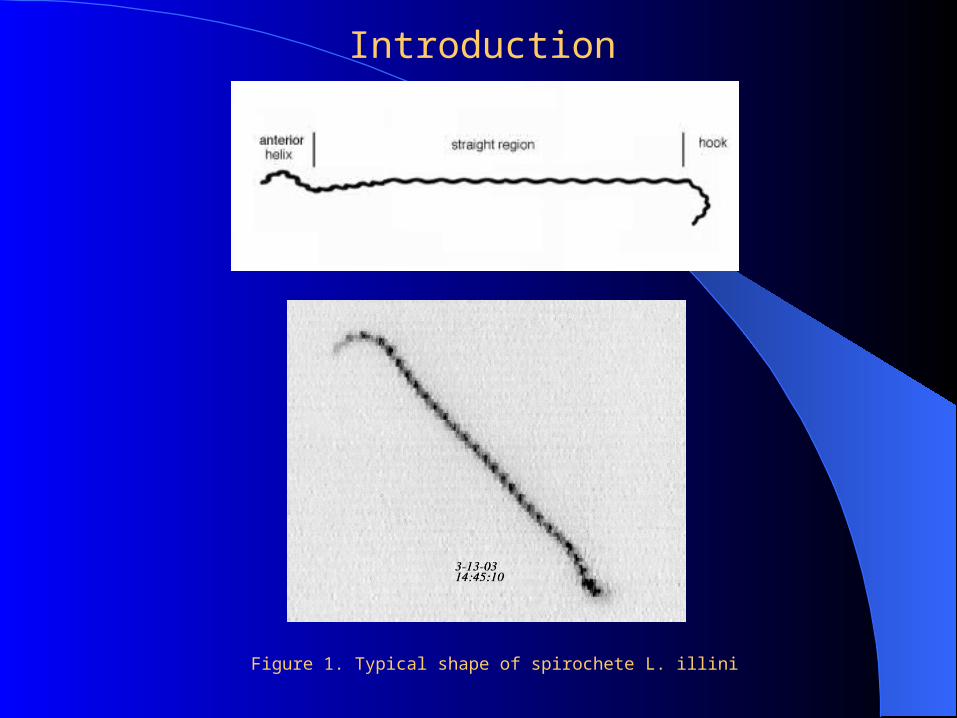
Figure 1. Typical shape of spirochete L. illini
Introduction

Axial filament involvement in the motility of Leptospira interrogans. DB Bromley and N W Charon
Introduction

Dynamics of spirochete L. illini (Professor Stuart Goldstein Department of Genetics and Cell Biology at the University of Minnesota)
Introduction

SummarySummary
Model of the geometryModel of the mechanical motion Fluid dynamics of the spirocheteNumerical resultsDynamical simulations
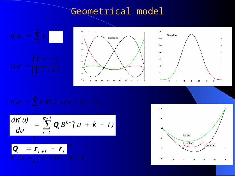
Geometrical modelGeometrical model
)u(L)u( i
m
1ii
rr
ijji
ijj
i )uu(
)uu(
)u(L
)1u3u3u(61
)u(B
)4u6u3(61
)u(B
)1u3u3u3(61
)u(B
u61
)u(B
2333i
2332i
2331i
33i
)i)1k(u(B)u(m
1i
ki
rr
1m
1i
1ki )iku(B
du)u(d
Qr
i1ii rrQ

s)s(z),wssin()s(R)s(y),wscos()s(R)s(x
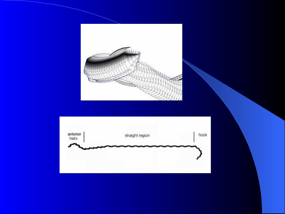
Step 1: Flagella along the whole body length
Step 2: Superhelix on top of the flagella
Geometrical modelGeometrical model
Torsion:
11 s
0
111
s
0
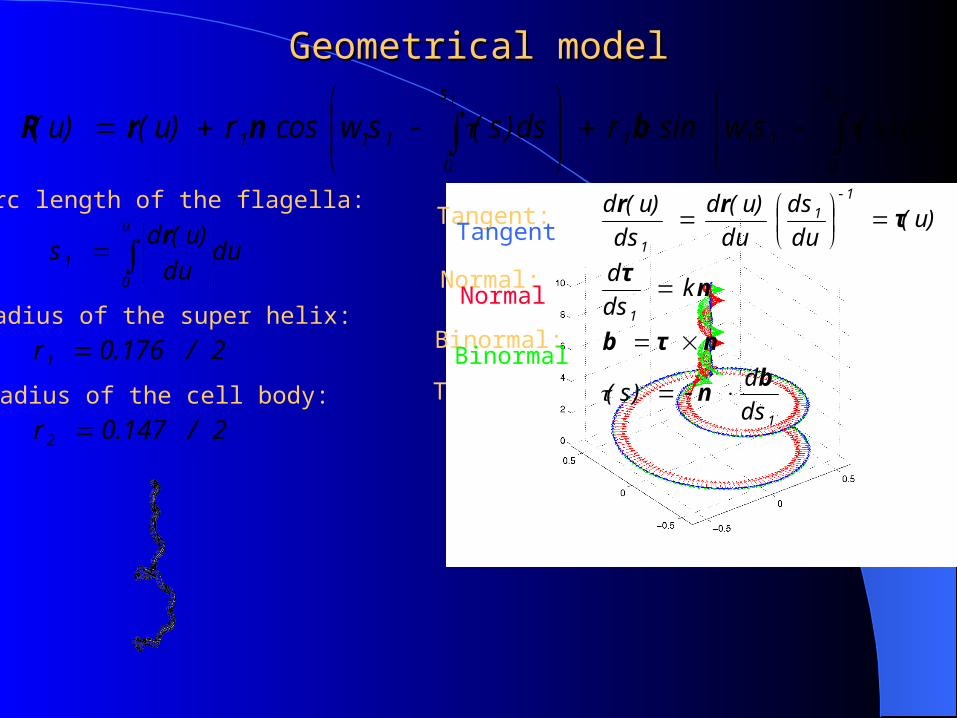
111 ds)s(swsinrds)s(swcosr)u()u( bnrR
Radius of the super helix:
dudu
)u(ds
u
0
1 r
1
1
11
1
dsd
)s(
kdsd
)u(duds
du)u(d
ds)u(d
bn
nτb
nτ
τrr
Geometrical modelGeometrical model
2/0.176r1
Arc length of the flagella:
Radius of the cell body:
2/0.147r2
Tangent:
Normal:
Binormal:
Tangent
Normal
Binormal

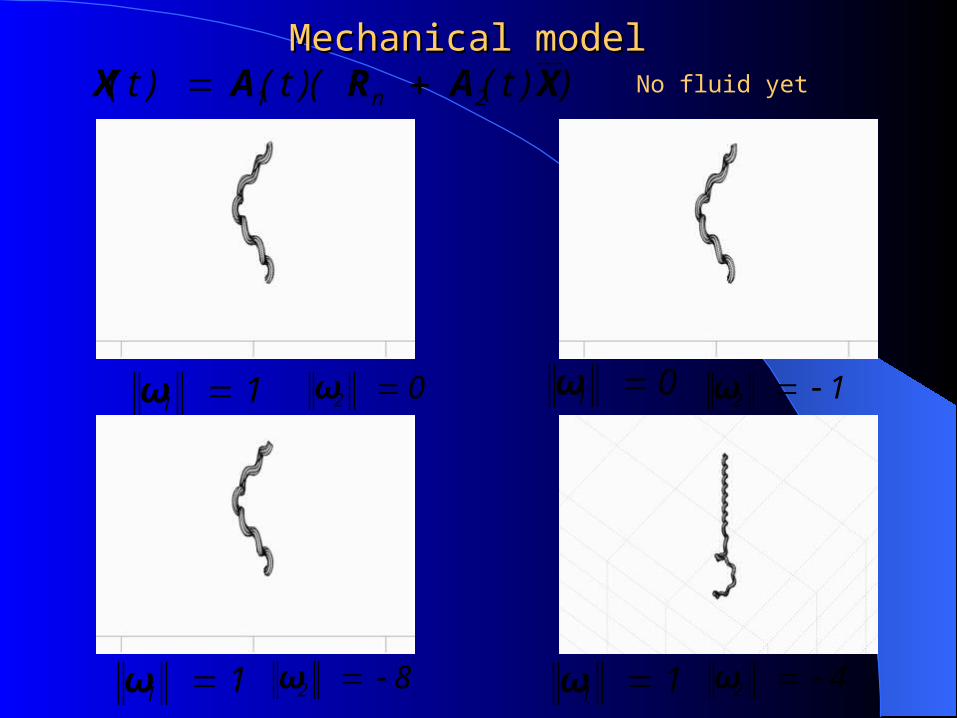
Mechanical model Mechanical model
z11 eωω τωω 22
))t()(t()t( 2n1 XARAX
XωXRωv 2n1 )()t(
2sin~
2cos
2sin~2
xIxIA
Reduce number of parameters describing the system (DoF) totwo rotations and translation
Rotation about vertical center line (0,0,1):
Rotation about tangent vector:
Rodrigues rotation matrix:
0xx
x0x
xx0~
12
13
23
xzor eτx where
Coordinate and velocity of a point on the surface:
X - coordinate in the “moving frame” coordinate system
))t()(t()t( 2n1 XARAX Mechanical model Mechanical model
02 ω11 ω 12 ω01 ω
82 ω11 ω 42 ω11 ω
No fluid yet

)s()s( 22 τωω
Mechanical model Mechanical model
XωXRωv 2n1 )()t(
Velocity distribution due to rotation about tangent vectors of the flagellum:
z11 eωω
12 ω
01 ω
)s(τ

0L~VL~L~0F~VF~F~
3z
2z2
1z1
3z
2z2
1z1
Mechanical model Mechanical model

Fluid mechanics of the swimming spirochete Fluid mechanics of the swimming spirochete
j
j
j
iijij x
)(u
x)(u
)(p)(xx
xx
3
1iiijj )(n)()(f xxx
D),()()()(
0
p
321
xxvxvxvxu
u
0σuStokes equation for the velocity of the fluid is LINEAR equation!
Hydrodynamical forces
where
- hydrostatic pressurep
- stress tensor

)( nz11 XRev
Xτv 22
z3 Vev
D
)(ds)( xxfF
D
)(ds)( xxfxL
0L~VL~L~0VFF~F~
3z
2z2
1z1
3z
2z2
1z1
Fluid mechanics of the swimming spirochete Fluid mechanics of the swimming spirochete
We compute distribution of hydrodynamical forces over the surface for each boundary condition,and compute total force and moment
If motion is steady state – sum of forces and moments equal to zero:
Because Stokes equation is linear
)1(V)V(),1()(
)1(V)V(),1()(
2,12,1
2,12,1
LLLL
FFFF

Stokes equations can be resolved in terms of Stokeslets
3
1i
2i,0i
3j,0ji,0iij
0ij
)xx(||||r
,r
)xx)(xx(
r),(G
r
xx
3
1i
-iiD 0ij0j )(S))d(f-)(f(),(G
81
)(u xxxxxx
Fluid mechanics of the swimming spirochete Fluid mechanics of the swimming spirochete

R. Cortez, L. Fauci, A. Medovikov The method of regularized stokeslets in three dimensions: analysis, validation, and application to helical swimming. Physics of Fluids 17, 031504 2005(also March 1, Volume 9, Issue 5, 2005 of Virtual Journal of Biological Physics Research)
2/722
4
)r(815
)(
x
)(ds)ff(),(G81
V)()(uV)()(u
3
1iiiD 0ij,
0D j0D\V j
xxx
dxxxdxxx
2/322j,0ji,0i
2/322
22
ij0ij, )r(
)xx)(xx(
)r()2r(
),(G
xx
where
is regularized Stokeslet
The method of regularized Stokeslets in three dimensionsThe method of regularized Stokeslets in three dimensions

Approximating of the regularized integral equation obtain local error estimate
10j0D j0D\V j Err)(uV)()(uV)()(u xdxxxdxxx
)(Oss
ErrErr),s,(Err3
3
3
3
21
)(ds)ff(),(G81 3
1iiiD 0ij, xxx
r
1
3
1i2
ppppppppi00ppij,00j Errws),s(J),s(f),s,,s(G
81
),s(u
2/5)x,D(distif,2
2/5)x,D(distif,1where
0
0
The method of regularized Stokeslets in three dimensionsThe method of regularized Stokeslets in three dimensions
r
1
3
1i ppppppppi00ppij,00j ws),s(J),s(f),s,,s(G
81
),s(u
FU
A
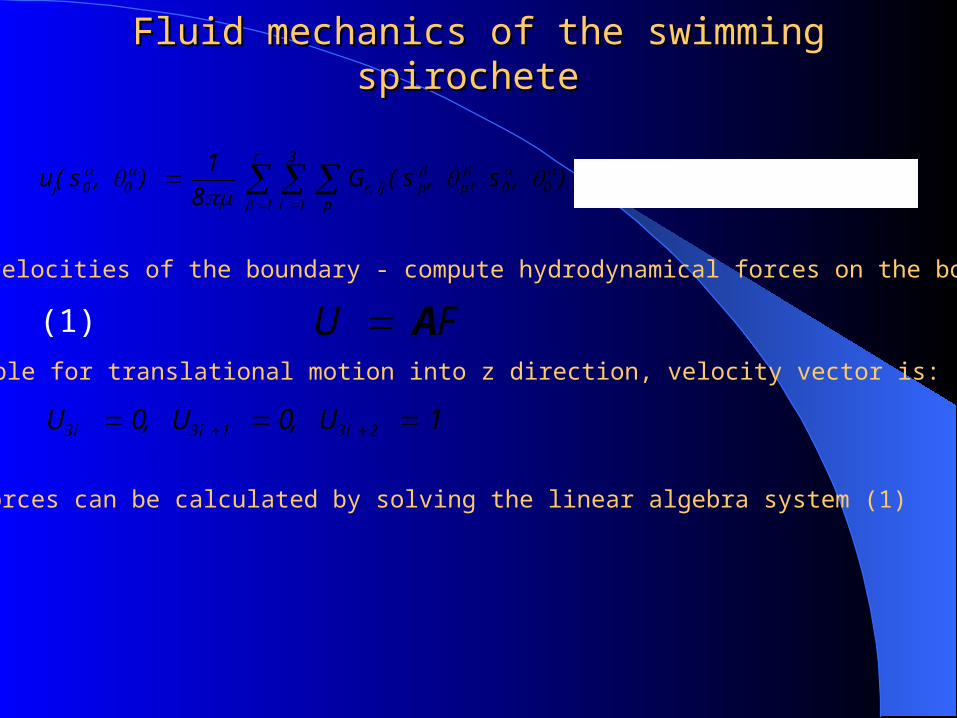
Fluid mechanics of the swimming spirochete Fluid mechanics of the swimming spirochete
Given velocities of the boundary - compute hydrodynamical forces on the boundary
1U,0U,0U 2i31i3i3
For example for translational motion into z direction, velocity vector is:
and forces can be calculated by solving the linear algebra system (1)
(1)

Numerical ResultsNumerical Results
Velocity field of the liquid
3
1iiD 0ij0j )(S)d(f),(G
81
)(u xxxxx

Numerical ResultsNumerical Results
1z
3z1
3z
1z1
F~F~
V
0F~VF~
0L~VL~L~0F~VF~F~
3z
2z2
1z1
3z
2z2
1z1

0L~VL~L~0F~VF~F~
3z
2z2
1z1
3z
2z2
1z1
Numerical ResultsNumerical Results
Balance of forces and moments along z direction for steady-state motion
Numerical ResultsNumerical Results
0L~VL~L~0F~VF~F~
3z
2z2
1z1
3z
2z2
1z1
1z
2z
2z
1z
1z
3z
3z
1z
1
1z
2z
2z
1z
3z
2z
2z
3z
LFLFLFLF
v
LFLFLFLF
v
1LFLFLFLF3z
2z
2z
3z
1z
3z
3z
1z1
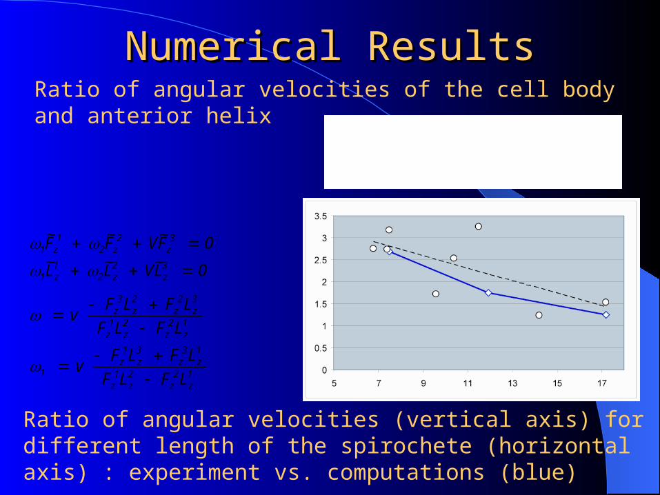
Ratio of angular velocities (vertical axis) for different length of the spirochete (horizontal axis) : experiment vs. computations (blue)
Ratio of angular velocities of the cell body and anterior helix

Dynamical ModelDynamical Model
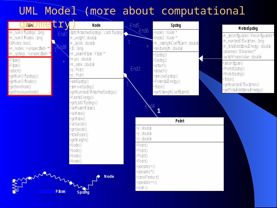
We approximate surface by network of connected springs
+reconfigure()+MotorSpring()+MotorSpring()+force()+getNumberOfSwitches()+getTotalAdditionalEnergy()
-m_reconfigurator : Reconfigurator *-m_numberOfSwitches : long-m_totalAdditionalEnergy : double-observer : IObserver *-switchForceValue : double
MotorSpring
+addSpring()+removeSpring()+getNumberOfAttachedSprings()+KineticEnergy()+getListOfSprings()+setParentFibre()+setArea()+getArea()+setJacob()+getJacob()+totalForce()+getWeight()+Node()+Node()+Node()+Node()
-listOfAttachedSprings : ListOfSprings-m_weight : double-m_jacob : double+ID : long+m_parentFibre : Fibre *+mass : double+m_area : double+q : Point+p : Point
Node
+Point()+Point()+Point()+Point()+operator =()+operator *()+crossProduct()+operator ==()+norm()
+x : double+y : double+z : double
Point
+Spring()+Spring()+attach()+detach()+removeSpring()+PotentialEnergy()+force()+getStrengthCoefficient()
+node1 : Node *+node2 : Node *+m_strengthCoefficient : double+restLength : double
Spring
-End3
1
-End4
1
-End5
1
-End6
*
+Fibre()+Fibre()+attach()+getNumOfSprings()+getNumOfNodes()+getNextNode()+getPreviouseNode()
+m_numOfSprings : long+m_numOfNodes : long+isMotor : bool+m_nodes : <unspecified> **+m_springs : <unspecified> **
Fibre
-End7
1-End8
*
Spring
Node
Fibre
1
UML Model (more about computational geometry)
+CCreatureBase()+~CCreatureBase()
CCreatureBase
+RingCreature()+RingCreature()+~RingCreature()+CollectNodes()+CollectVelocityNodes()+RotateRing()
+m_numOfSprings : int+m_numOfNodes : int+m_numOfVelocityNodes : int+m_velocityNodes : Node **+m_nodes : Node **+m_SprCoeffForIntRg : double+m_TotalMassOfRing : double+m_centerInfos : vector<RingCenterInfo>+forceRings : vector<Ring*>+velicityRings : vector<Ring*>+totalNumOfNodes : long+totalNumOfVelocityNodes : long
RingCreature
+MotorRing()+attachMotors()+reAttachMotors()+setStrengthCoefficientOfMotor()+getMotorSprings()+~MotorRing()
-m_motorSprings : MotorSpring **-motorOn : bool-strengthCoefficientOfMotor : double+numOfSwitches : long
MotorRing
-setTransformationMatrix()+Ring()+~Ring()+getRadius()+getStrengthCoefficient()+getNormal()+getCenter()+setCenter()+setNormal()+refreshCenter()+attach()+moveTo()+getNextNode()+getPreviouseNode()
-m_angle : double-m_radius : double-m_strengthCoefficient : double-m_normal : Point-m_center : Point-m_mass : double-m_transformationMatrix[3] : Point
Ring
-End1
1
-End2
*
+CenterLine()+CenterLine()+GetCentralLine()+lagrange()+interpolation()+tangent()+BSplineBasis()+BSplineDerivative()+BSpline2Derivative()+BSpline3Derivative()+dRds()+d2Rd2s()+d3Rd3s()+getRecursiveBSpline()+Flagella()
#radius : double+m_order : int
CenterLine
+GetCentralLine()+StaticCenterLine()+getFrameRotationalMatrix()
+m_RadiusOfFlagella : double+m_numOfPoints : int+flagellaCenters : vector<Point>+spiroCenters : vector<Point>+flagellaTangents : vector<Point>+spiroTangents : vector<Point>
StaticCenterLine
+Fibre()+Fibre(in numOfNodes : long, in numOfSprings : long)+attach(in fibre : Fibre*, in connector : <unspecified>*) : <unspecified> *+getNumOfSprings() : long+getNumOfNodes() : long+getNextNode(in ID : long) : <unspecified> *+getPreviouseNode(in ID : long) : <unspecified> *
+m_numOfSprings+m_numOfNodes+isMotor+m_nodes+m_springs
Fibre
1
Ring
N+1 N+1
N
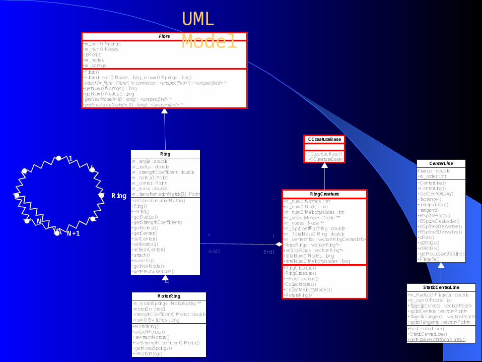
UML Model

Dynamical ModelDynamical Model
We approximate the initial intrinsic shape of the spirochete by a network of points and springs.
We use the boundary integral equations to calculate the surface velocities of elastic structures in Stokes fluid from surface elastic forces
The regularized Stokeslet method allows us to overcome difficulties related to the weak singularities of the boundary integral formulation
Numerical approximation leads to system of stiff ordinary differential equations, which we solve by DUMKA3 -a fast explicit solver for stiff ordinary differential equations

Because
ux
dt
)t(d
r
1
3
1i ppi0ij,
j w~)(f),(G8
1
dt
dx
xxx
Dynamical ModelDynamical Model
)X(F)X(dtXd
elastic
A
Dynamical problem is a system of ODEs:
Where is calculated from elastic and geometrical properties of the surfaceelasticF

To solve system of ODE we use fast explicit DUMKA3 -a fast explicit solver for stiff
ordinary differential equations
n
ii
n
iin
n
ii
n
iin
nPnh
ASpP
hyy
1
'
1
110
)0(/
)(1|)1(||)(|
)1(
as large as possible


D,vvv)(u
,0x
)(u
,0x
)(
x)(p
)(u
3i
2i
1ii
3
1i i
i
3
1j j
ij
ii
xx
ux
xxx
r
1 ppppppppij ws),s(J),s(fF

)i)1k(u(B)u(m
1i
ki
rr
1m
1i
1ki )iku(B
du)u(d
Qr
i1ii rrQ
1)u(Bi
)y(max)u(y)y(min
)x(max)u(x)x(min
jij3i
jij3i
jij3i
jij3i
)1u3u3u(61
)u(B
)4u6u3(61
)u(B
)1u3u3u3(61
)u(B
u61
)u(B
2333i
2332i
2331i
33i

From: Mark DePristo's notes on biology: raven.bioc.cam.ac.uk/~mdepristo/

R F
0.01 0.201135
0.1 0.168359
0.2 0.119337
0.3 -0.137456
0.4 -0.128172
0.5 -0.37992

Rotation of a fragment of the spirochete about flagellum tangent vectors with angular velocity (a), rotation of the spirochete about with angular velocity (b) (view is taken from the point (0.8,0,13)).
)s( it 11 ze
1

Combination of rotations: , (a); , (b); , (c); (view is taken from the point (-3,3,14)).
11 1 01 111 0

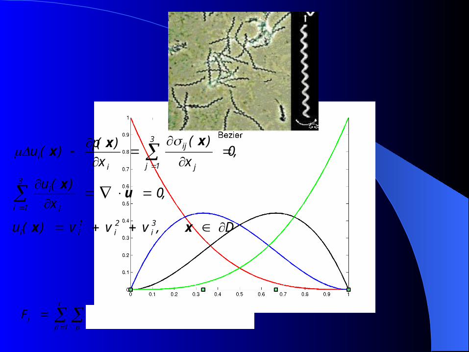
A spirochete is a bacterium with a characteristic helical, elastic body. Because of its unique structure, a spirochete can swim in highly viscous, gel-like media, such as collagen within the mammal, and mucosal surfaces. Several species of spirochetes cause medically important diseases, some with grave consequences: Weil's disease, syphilis, yaws, bejel, pinta, Lyme disease (which is the most prevalent vector-borne disease in the United States), relapsing fever, leptospirosis and more. The spirochete is composed of different connected parts that have complicated shapes (several flagella, elastic spirochete's body, outer sheath and motors). We consider three aspects of the model: model of the geometry, model of the mechanical motion and the regularized Stokeslet method for simulation of fluid dynamics of the spirochete. We investigate the role of the geometry for the swimming and how we can compute global measurable characteristics of the motion.