Embed Size (px)
Citation preview
HAL Id: hal-00778412https://hal.inria.fr/hal-00778412
Submitted on 20 Jan 2013
HAL is a multi-disciplinary open accessarchive for the deposit and dissemination of sci-entific research documents, whether they are pub-lished or not. The documents may come fromteaching and research institutions in France orabroad, or from public or private research centers.
L’archive ouverte pluridisciplinaire HAL, estdestinée au dépôt et à la diffusion de documentsscientifiques de niveau recherche, publiés ou non,émanant des établissements d’enseignement et derecherche français ou étrangers, des laboratoirespublics ou privés.
Numerical Simulation of Piecewise-Linear Models ofGene Regulatory Networks Using Complementarity
SystemsVincent Acary, Hidde de Jong, Bernard Brogliato
To cite this version:Vincent Acary, Hidde de Jong, Bernard Brogliato. Numerical Simulation of Piecewise-Linear Modelsof Gene Regulatory Networks Using Complementarity Systems. [Research Report] RR-8207, INRIA.2013, pp.42. hal-00778412
ISS
N02
49-6
399
ISR
NIN
RIA
/RR
--82
07--
FR+E
NG
RESEARCHREPORTN° 8207January 19, 2013
Project-Teams Bipop and Ibis
Numerical Simulation ofPiecewise-Linear Modelsof Gene RegulatoryNetworks UsingComplementaritySystemsVincent Acary, Hidde de Jong, Bernard Brogliato

RESEARCH CENTREGRENOBLE – RHÔNE-ALPES
Inovallée655 avenue de l’Europe Montbonnot38334 Saint Ismier Cedex
Numerical Simulation of Piecewise-LinearModels of Gene Regulatory Networks Using
Complementarity Systems
Vincent Acary∗, Hidde de Jong∗, Bernard Brogliato∗
Project-Teams Bipop and Ibis
Research Report n° 8207 — January 19, 2013 — 39 pages
Abstract: Gene regulatory networks control the response of living cells to changes in theirenvironment. A class of piecewise-linear (PWL) models, which capture the switch-like interactionsbetween genes by means of step functions, has been found useful for describing the dynamics ofgene regulatory networks. The step functions lead to discontinuities in the right-hand side of thedifferential equations. This has motivated extensions of the PWL models based on differential in-clusions and Filippov solutions, whose analysis requires sophisticated numerical tools. We present amethod for the numerical analysis of one proposed extension, called Aizermann-Pyatnitskii (AP)-extension, by reformulating the PWL models as a mixed complementarity system (MCS). Thisallows the application of powerful methods developed for this class of nonsmooth dynamical sys-tems, in particular those implemented in the Siconos platform. We also show that under a set ofreasonable biological assumptions, putting constraints on the right-hand side of the PWL models,AP-extensions and classical Filippov (F)-extensions are equivalent. This means that the proposednumerical method is valid for a range of different solution concepts. We illustrate the practicalinterest of our approach through the numerical analysis of three well-known networks developedin the field of synthetic biology.
Key-words: Nonsmooth dynamical systems, gene regulatory networks, piecewise-linear models,Filippov solutions, differential inclusions, complementarity systems
Simulation numerique des modeles lineaires par morceauxde reseaux de regulation geniques par des systemes de
complementarite
Resume : Les reseaux de regulation genique commandent la reponse des cellulles vivantesaux changements de leur environnement. Une famille de modeles lineaires par morceaux quimodelisent les interactions de type “commutation” entre les genes au moyen de fonctions sauts,s’est revelee utile pour decrire la dynamique des reseaux de regulation genique. Les fonc-tions sauts conduisent a des equations differentielles discontinues. Ceci a motive l’ecriture desmodeles lineaires par morceaux comme des inclusions differentielles et a chercher des solutionsau sens de Filippov, dont la simulation demande des outils numeriques sophistiques. Nouspresentons une methode numerique pour une extension sous forme d’inclusion differentielle ditede Aizermann-Pyatnitskii, en reformulant les modeles lineaires par morceaux comme des systemesde complementarite mixtes. Cela permet l’application de methodes efficaces developpees pourcette classe de systemes dynamiques non reguliers, en particulier celles developpees dans le logicielSiconos. Nous montrons aussi sous des hypotheses raisonnables d’un point de vue biologique quel’extension de Aizermann-Pyatnitskii et l’extension de Filippov sont equivalentes. Cela impliqueque cette methode numerique est pertinente pour une grande classe de notions de solutions. Nousillustrons l’interet pratique de cette approche a travers l’analyse numerique de trois reseaux bienconnus dans le domaine de la biologie synthetique.
Mots-cles : Systemes dynamiques non reguliers, reseaux de regulation genique, modeleslineaires par morceaux, solutions de Filippov, inclusions differentielles, systemes de complementarite.
Numerical Simulation of Piecewise-Linear Models of Gene Regulatory Networks 3
1 Introduction
When confronted with changing environmental conditions, living systems have a remarkablecapacity to rapidly adapt their functioning. For instance, the response of a bacterial cell to thedepletion of an essential nutrient leads to the upregulation and downregulation of the expressionof up to several hundreds of genes [45]. The genes encode enzymes, transcription regulators,membrane transporters and other macromolecules playing a role in cellular processes. The controlof the adjustment of gene expression levels is achieved by so-called gene regulatory networks,consisting of genes, RNAs, proteins, and their mutual regulatory interactions.
In order to understand how a particular network structure brings about observed changes ingene expression, mathematical models in combination with computer simulation are increasinglyused, especially in the emerging field of systems biology [11]. The modeling of gene regulatorynetworks also plays a prominent role in synthetic biology, which aims at designing a networkstructure capable of producing a desired gene expression pattern, for instance a robust oscillationor an externally controlled switch [51]. The networks may be constructed de novo or obtainedby rewiring a natural regulatory network.
A variety of formalisms are available for modeling gene regulatory networks [18, 50]. Formany purposes, approximate models based on simplifications of classical kinetic models havebeen proven useful [24, 28, 41]. First, the approximate models are easier to calibrate againstexperimental data, due to the fact that they reduce the number of parameters and the complexityof the rate equations. This may help relieve what is currently a bottleneck for modeling insystems biology, namely obtaining reliable estimates of parameter values. Second, the simplifiedmathematical form of the models makes them easier to analyze. Among other things, this makesit possible to single out the precise role of specific subnetworks [1, 67] and to analyze the feasibilityof control schemes [32].
In this paper we look at one particular class of approximate models of gene regulatory net-works, so-called piecewise-linear (PWL) models [39]. The PWL models are systems of coupleddifferential equations in which the variables denote concentrations of gene products, typicallyproteins. The rate of change of a concentration at a particular time-point may be regulated byother proteins through direct or indirect interactions. The PWL models capture these regulatoryeffects by means of step functions that change their value in a switch-like manner at thresholdconcentrations of the regulatory proteins. The step functions are approximations of the sigmoidalresponse functions often found in gene regulation.
PWL models with step functions have favorable mathematical properties, which allows forthe analysis of steady states, limit cycles, and their stability [23, 31, 35, 40]. The use of stepfunctions, however, leads to discontinuities in the right-hand side of the differential equations,due to the abrupt changes of the value of a step function at its threshold. These discontinuitiesare sometimes ignored, which is potentially dangerous as it may cause steady states and otherimportant dynamical properties of the system to be missed. In order to deal with the discon-tinuities, several authors have proposed the use of differential inclusions and Filippov solutions[37, 42, 53]. These proposals to extend PWL models to differential inclusions differ in subtle butnontrivial ways, giving rise to systems with nonequivalent dynamics [53].
Currently, only few computational tools are available to support the analysis of the differ-ential inclusions obtained from Filippov extensions of PWL models. Genetic Network Analyzer(GNA) provides a qualitative analysis of PWL models of gene regulatory networks (e.g., [13, 14]).However, the analysis is based on hyperrectangular overapproximations of the differential inclu-sions proposed in [37], and it is currently not clear to which extent this introduces artifacts in theanalysis. Moreover, the predictions obtained from this analysis are purely qualitative, describingpossible transitions between state-space regions rather than giving numerical solutions. Alterna-
RR n° 8207
4 Acary, V., de Jong, H. & B. Brogliato
tively, an algorithm based on the use of steep sigmoidal response functions in combination withsingular perturbation theory has been presented [47].
The aim of this paper is to propose a theoretically sound and practically useful method forthe numerical simulation of gene regulatory networks described by PWL models. We notablyshow that the Aizerman & Pyatnitskii extension (see [37, Definition c), page 55] or [9]) ofPWL models can be reformulated in the framework of complementarity systems or differentialvariational inequalities [4, 44, 57]. The Aizerman & Pyatnitskii extension has been introducedin the context of PWL models of gene regulatory networks in [53], where it is shown that itleads to a more restrictive extension than the standard Filippov extension. The reformulationas a complementarity system allows us to employ the rich store of numerical methods availablefor these and other classes of discontinuous systems [2, 4]. Moreover, we show that under tworeasonable biological assumptions, posing constraints on the admissible network structures, thedifferent extensions of PWL models that have been proposed, as well as the hyperrectangularoverapproximation in [14], are equivalent. This means that the numerical simulation approachdeveloped in this paper is valid for a range of different solution concepts for PWL models of generegulatory networks.
We illustrate the interest of our numerical simulation approach by means of the analysis ofthree synthetic networks published in the literature: the repressilator [33], an oscillator withpositive feedback [12], and the IRMA network [22]. We develop PWL models of these networks,either from scratch or by adapting existing ODE models, and numerically simulate the dynamicresponse of these networks to external stimuli. The simulations are shown to reproduce knownqualitative features of these networks, notably the capability to generate (damped) oscillationsfor the first two networks, and a switch-on/switch-off response after a change in growth mediumfor the third. We believe these examples demonstrate that the numerical simulation approachdeveloped in this paper provides a useful extension of the toolbox of modelers of gene regulatorynetworks.
2 PWL models of gene regulatory networks
2.1 Definition of PWL models
The dynamics of genetic regulatory networks can be described by piecewise-linear (PWL) differ-ential equation models using step functions to account for regulatory interactions [26, 39, 55]. Inthis section we briefly summarize the PWL modeling framework.
We denote by x = (x1, . . . , xn)T ∈ Ω a vector of cellular protein or RNA concentrations,where Ω ⊂ Rn+ is a bounded n-dimensional hyperrectangular subspace of Rn+. For each concen-tration variable xi, i ∈ 1, . . . , n, we distinguish a set of constant, strictly positive thresholdconcentrations θ1
i , . . . , θpii , pi > 0. At its thresholds a protein may affect the expression of genes
encoding other proteins or the expression of its own gene. We call Θ =⋃i∈1,...,n,k∈1,...,pix ∈
Ω | xi = θki the subspace of Ω defined by the threshold hyperplanes.
Definition 1 (PWL model). A PWL model of a gene regulatory network is defined by a set ofcoupled differential equations
xi = fi(x) = −γi xi + bi(x) = −γi xi +∑l∈Li
κli bli(x), i ∈ 1, . . . , n, (1)
where κli and γi are positive synthesis and degradation constants, respectively, Li ⊂ N are sets ofindices of regulation terms, and bli : Ω \Θ→ 0, 1 are so-called regulation functions.
Inria
Numerical Simulation of Piecewise-Linear Models of Gene Regulatory Networks 5
Intuitively, (1) defines the rate of change of each concentration xi as the difference of the rateof synthesis (the first term in the right-hand side) and the rate of degradation (the second term).The synthesis term depends on the concentrations of regulatory proteins through the regulationfunctions, which account for the interactions between the genes in the network. Degradation isdescribed by a first-order term including contributions of growth dilution and protein degrada-tion. While this is sufficient for the examples treated in this paper, the degradation term in (1)can be easily extended to include proteolytic regulators.
Each regulation function bli(·) is defined in terms of step functions
s+(xj , θkj )=
1 if xj > θkj0 if xj < θkj
and s−(xj , θkj )=
0 if xj > θkj1 if xj < θkj
, (2)
where xj is a concentration variable, j ∈ 1, . . . n, and θkj a threshold for xj , k ∈ 1, . . . pi.Notice that s−(xj , θ
kj ) = 1 − s+(xj , θ
kj ). The step functions capture the switch-like character
of gene regulation by transcription factors and other proteins. The regulation functions arealgebraic equivalents of discrete Boolean functions expressing the combinatorial logic of generegulation [66].
For future use, we introduce the following generalizations of the step functions s+(xj , θkj ) and
s−(xj , θkj ), which consists of extending the function at the discontinuities:
S+(xj , θkj ) =
1 xj > θkj[0,1] xj = θkj0 xj < θkj
and S−(xj , θkj ) =
0 xj > θkj[0,1] xj = θkj1 xj < θkj
. (3)
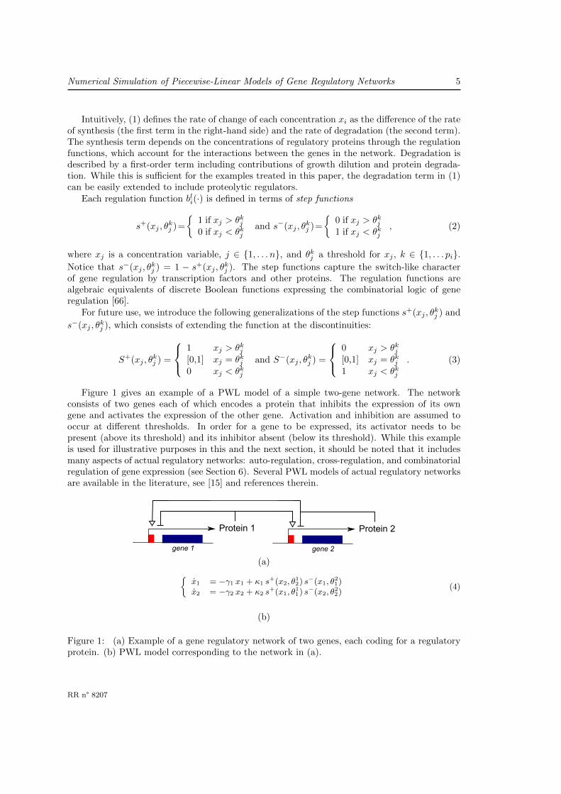
Figure 1 gives an example of a PWL model of a simple two-gene network. The networkconsists of two genes each of which encodes a protein that inhibits the expression of its owngene and activates the expression of the other gene. Activation and inhibition are assumed tooccur at different thresholds. In order for a gene to be expressed, its activator needs to bepresent (above its threshold) and its inhibitor absent (below its threshold). While this exampleis used for illustrative purposes in this and the next section, it should be noted that it includesmany aspects of actual regulatory networks: auto-regulation, cross-regulation, and combinatorialregulation of gene expression (see Section 6). Several PWL models of actual regulatory networksare available in the literature, see [15] and references therein.
Protein 1
gene 1
Protein 2
gene 2
(a)x1 = −γ1 x1 + κ1 s
+(x2, θ12) s
−(x1, θ21)
x2 = −γ2 x2 + κ2 s+(x1, θ
11) s
−(x2, θ22)
(4)
(b)
Figure 1: (a) Example of a gene regulatory network of two genes, each coding for a regulatoryprotein. (b) PWL model corresponding to the network in (a).
RR n° 8207
6 Acary, V., de Jong, H. & B. Brogliato
2.2 Regulation functions in PWL models
Which regulation functions bli(·) entering the PWL models are admissible? In order to answerthis question, we first develop how the regulation functions relate to Boolean functions describingthe combinatorial control of gene regulation.
Recall that each variable xj has pj thresholds θ1j , . . . , θ
pjj . The step functions can be
associated with Boolean variables Xkj such that
Xkj (x) = (xj > θkj ) = s+(xj , θ
kj )
Xkj (x) = (xj < θkj ) = s−(xj , θ
kj ),
(5)
where X denotes the complemented variable of X.
Let us give some basic definitions of Boolean algebra [52, Chapter 3]. A literal denoted byYj is defined either as the Boolean variable Yj or its negation Yj . Given a set of n Booleanvariables Y1, . . . , Yn, a minterm m is defined as a conjunction of exactly n literals in whicheach Yj , j ∈ 1 . . . n appears once (each variable appears once in either its complemented oruncomplemented form). That is,
m =
n∏j=1
Yj . (6)
For the set of variables Xkj , j ∈ 1, . . . , n, k ∈ 1, . . . , pj, we have 2p minterms, with p =∑
j∈1,...,n pj , and these are denoted as
mα(x) =
n∏j=1
pj∏k=1
X kj (x), α ∈ 0, . . . , 2p − 1. (7)
The subscript α corresponds to the decimal equivalent of the conventional binary encoding ofliterals (1 for Xk
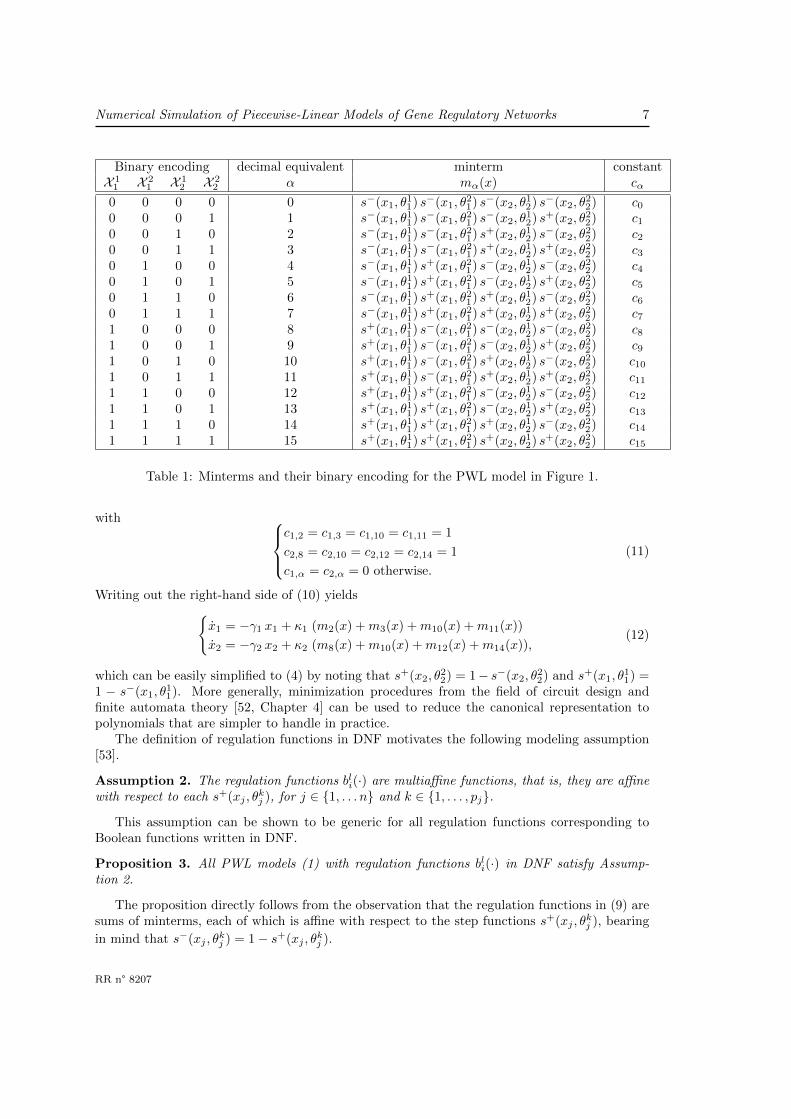
j and 0 for Xkj ). Table 1 gives an example of the minterms for the four variables
in the example of Figure 1, with their corresponding binary encoding and decimal equivalent.
Regulation functions can now be defined as the minterm expression of a Boolean function[59]. More precisely, they can be rewritten in minterm disjunctive normal form (DNF):
bli(x) =
2p−1∑α=0
cli,αmα(x), (8)
with cli,α ∈ 0, 1. By means of (8), the PWL models can be written as
xi = fi(x) = −γi xi +∑l∈Li
κli
2p−1∑α=0
cli,αmα(x), i ∈ 1, . . . , n. (9)
As an example, consider the DNF of the regulation functions in the PWL model of Figure 1.Since L1 = L2 = 1, we omit the superscript l for κli and cli,α. As each variable has two thresholds,the canonical representation is composed of the 16 minterms shown in Table 1. Notice that foreach state variable x1, x2, only 4 of the coefficients ci,α equal 1. We thus obtain the followingPWL model:
x1 = −γ1 x1 + κ1
∑15α=0 c1,αmα(x)
x2 = −γ2 x2 + κ2
∑15α=0 c2,αmα(x),
(10)
Inria
Numerical Simulation of Piecewise-Linear Models of Gene Regulatory Networks 7
Binary encoding decimal equivalent minterm constantX 1
1 X 21 X 1
2 X 22 α mα(x) cα
0 0 0 0 0 s−(x1, θ11) s−(x1, θ
21) s−(x2, θ
12) s−(x2, θ
22) c0
0 0 0 1 1 s−(x1, θ11) s−(x1, θ
21) s−(x2, θ
12) s+(x2, θ
22) c1
0 0 1 0 2 s−(x1, θ11) s−(x1, θ
21) s+(x2, θ
12) s−(x2, θ
22) c2
0 0 1 1 3 s−(x1, θ11) s−(x1, θ
21) s+(x2, θ
12) s+(x2, θ
22) c3
0 1 0 0 4 s−(x1, θ11) s+(x1, θ
21) s−(x2, θ
12) s−(x2, θ
22) c4
0 1 0 1 5 s−(x1, θ11) s+(x1, θ
21) s−(x2, θ
12) s+(x2, θ
22) c5
0 1 1 0 6 s−(x1, θ11) s+(x1, θ
21) s+(x2, θ
12) s−(x2, θ
22) c6
0 1 1 1 7 s−(x1, θ11) s+(x1, θ
21) s+(x2, θ
12) s+(x2, θ
22) c7
1 0 0 0 8 s+(x1, θ11) s−(x1, θ
21) s−(x2, θ
12) s−(x2, θ
22) c8
1 0 0 1 9 s+(x1, θ11) s−(x1, θ
21) s−(x2, θ
12) s+(x2, θ
22) c9
1 0 1 0 10 s+(x1, θ11) s−(x1, θ
21) s+(x2, θ
12) s−(x2, θ
22) c10
1 0 1 1 11 s+(x1, θ11) s−(x1, θ
21) s+(x2, θ
12) s+(x2, θ
22) c11
1 1 0 0 12 s+(x1, θ11) s+(x1, θ
21) s−(x2, θ
12) s−(x2, θ
22) c12
1 1 0 1 13 s+(x1, θ11) s+(x1, θ
21) s−(x2, θ
12) s+(x2, θ
22) c13
1 1 1 0 14 s+(x1, θ11) s+(x1, θ
21) s+(x2, θ
12) s−(x2, θ
22) c14
1 1 1 1 15 s+(x1, θ11) s+(x1, θ
21) s+(x2, θ
12) s+(x2, θ
22) c15
Table 1: Minterms and their binary encoding for the PWL model in Figure 1.
with c1,2 = c1,3 = c1,10 = c1,11 = 1
c2,8 = c2,10 = c2,12 = c2,14 = 1
c1,α = c2,α = 0 otherwise.
(11)
Writing out the right-hand side of (10) yieldsx1 = −γ1 x1 + κ1 (m2(x) +m3(x) +m10(x) +m11(x))
x2 = −γ2 x2 + κ2 (m8(x) +m10(x) +m12(x) +m14(x)),(12)
which can be easily simplified to (4) by noting that s+(x2, θ22) = 1− s−(x2, θ
22) and s+(x1, θ
11) =
1 − s−(x1, θ11). More generally, minimization procedures from the field of circuit design and
finite automata theory [52, Chapter 4] can be used to reduce the canonical representation topolynomials that are simpler to handle in practice.
The definition of regulation functions in DNF motivates the following modeling assumption[53].
Assumption 2. The regulation functions bli(·) are multiaffine functions, that is, they are affinewith respect to each s+(xj , θ
kj ), for j ∈ 1, . . . n and k ∈ 1, . . . , pj.
This assumption can be shown to be generic for all regulation functions corresponding toBoolean functions written in DNF.
Proposition 3. All PWL models (1) with regulation functions bli(·) in DNF satisfy Assump-tion 2.
The proposition directly follows from the observation that the regulation functions in (9) aresums of minterms, each of which is affine with respect to the step functions s+(xj , θ
kj ), bearing
in mind that s−(xj , θkj ) = 1− s+(xj , θ
kj ).
RR n° 8207
8 Acary, V., de Jong, H. & B. Brogliato
A second assumption requires that, when two genes have a common regulation, the latterdoes not act upon the two genes at the same threshold.
Assumption 4. Every step function s+(xj , θkj ), with j ∈ 1, . . . n and k ∈ 1, . . . , pj, oc-
curs in at most one bi(·), i ∈ 1, . . . , n. As a consequence, for a given j, k, every vector[∂bi(x)/∂s+
jk]i∈1,...,n, with s+jk ≡ s+(xj , θ
kj ), has at most one non-zero element.
Assumption 4 is a rather weak modeling assumption, in the sense that there is usually nocompelling biological reason for two genes to be regulated at exactly the same threshold. Thenotable exception is the case of bacterial genes co-transcribed from the same promoter, thatis, genes that are included in the same operon. Notice that all models of biological networkspresented in Section 6 satisfy Assumption 4.
The interest of the above restrictions on regulation functions, and thus on the right-hand sidesof the PWL models, is that together they entail the equivalency of different solution concepts.This will be shown in the next section.
3 Solutions of PWL models
3.1 Filippov extensions of PWL models
The use of step functions s±(xj , θkj ) in (9) gives rise to mathematical complications, because the
step functions are undefined and discontinuous at xj = θkj . Therefore, f(·) = (f1(·), . . . , fn(·))Tis undefined and may be discontinuous on the threshold hyperplanes Θ. In order to deal withthis problem, we can follow an approach originally proposed by Filippov [37] and widely usedin control theory. It consists in extending the differential equation x = f(x), x ∈ Ω \ Θ, to adifferential inclusion. Following the book of Filippov, Machina and Ponosov [53] review severaldifferent ways in which this can be done. Below we discuss the two main alternatives, whichwe call F- and AP-extensions, respectively, and we give precise definitions of the correspondingsolutions of the PWL models.
Definition 5 (F-extension of PWL models). The F-extension of the PWL model (1) is definedby the differential inclusion
x ∈ F(x), with F(x) = co
( limy→x, y 6∈Θ
f(y)), x ∈ Ω, (13)
where co(P ) denotes the closed convex hull of the set P , and limy→x, y 6∈Θ f(y) the set of alllimit values of f(y), for y 6∈ Θ and y → x.
This definition corresponds to the classical Filippov approach [37], as applied in the contextof gene regulatory network modeling in [42].
Formally, we define a F-PWL system Σ as the triple (Ω,Θ,F), that is, the set-valued functionF(·) given by (13), defined on the n-dimensional state space Ω, with Θ the union of the thresholdhyperplanes [14].
Definition 6. A solution of an F-PWL system Σ on a time interval I is a solution of thedifferential inclusion (13) on I, that is, an absolutely-continuous vector-valued function ξ(·) suchthat ξ(t) ∈ F(ξ(t)) almost everywhere on I.
For all x0 ∈ Ω and τ ∈ R+ ∪ ∞, ΞΣ(x0, τ) denotes the set of solutions ξ(t) of the PWLsystem Σ, for the initial condition ξ(0) = x0, and t ∈ [0, τ ]. In particular, notice that thederivative of ξ(·) may not exist, and therefore ξ(t) ∈ F(ξ(t)) may not hold, if ξ reaches or leaves
Inria
Numerical Simulation of Piecewise-Linear Models of Gene Regulatory Networks 9
Θ at t. The existence of at least one solution ξ on some time interval [0, τ ], τ > 0, with initialcondition ξ(0) = x0 is guaranteed for all x0 ∈ Ω [37]. However, in general there is not a uniquesolution.
As stated above, the book of Filippov proposes other extensions of the PWL systems, whichdo not define the right-hand side of the inclusion as the limit values of the function f(y), likein (13). A common definition of the right-hand side, following [37, Definition c), page 55], isattributed to [9] for systems of the form
x = f(x, u), x ∈ Rn, u ∈ Rp, (14)
where the function f : Rn+p → Rn is continuous in the set of arguments and u(x) : Rn → Rpis discontinuous. Systems (14) are often encountered in control theory, especially in variablestructure systems and sliding mode control [56, 69, 70]. At the point of discontinuity, for i 6= j,the arguments ui and uj of f are supposed to vary independently on the sets Ui(x) and Uj(x),usually assumed to be closed convex sets in R. The right-hand side of the differential inclusionin the sense of Aizerman and Pyatnitskii is then defined as
G(x) =y | y = f(x, u), ui ∈ Ui(x), i ∈ 1 . . . p
(15)
The set-valued vector field G(x) is generically non-convex and therefore often replaced by itsconvexification H(x) = co (G(x)). A standard result states that if f(·) in (14) is linear in u,then G(x) = H(x) if all Ui, i ∈ 1, . . . ,m, are convex [37, page 56] and [70]. Furthermore, ifthe arguments ui, i ∈ 1, . . . , p, are discontinuous on surfaces Si, such that the surfaces aredifferent and the normal vectors at the points of intersection are not linearly dependent, thenF(x) = G(x) = H(x).
In the context of the modeling of gene regulatory networks, Machina and Ponosov [53] applythe alternative extension G of the PWL models, using the generalized step functions S+(xj , θj)and S−(xj , θj) (Section 2.1) instead of the set-valued functions Ui. They argue that this ex-tension gives results that are closer to those obtained with gene regulatory network modelsusing sigmoidal functions rather than step functions, in the limit of infinitely-steep sigmoids [58].Moreover, as we will show below, this definition is more convenient for numerical simulationpurposes. We call the resulting differential inclusion the Aizerman-Pyatnitskii (AP)-extensionof PWL models.
Remark 7. In the seminal book of Filippov [37], G(·) is denoted as F1(·) and H(·) as F2(·). Inorder to avoid confusion with the components of F(·), we choose the alternative notation proposedhere.
Let σ = (σ11 , . . . , σ
p11 , . . . , σ1
n, . . . , σpnn )T ∈ [0, 1]p. Moreover, define the function g : Rp → Rn
by
gi(σ) =∑l∈Ln
κli bli(σ), j ∈ 1, . . . , n, (16)
where bli(·) are obtained from bli(·) by replacing every occurrence of s+(xj , θkj ) and s−(xj , θ
kj ) by
σkj and 1− σkj , respectively, for all j ∈ 1, . . . , n and k ∈ 1, . . . , pj.
Definition 8 (AP-extension of PWL models). The AP-extension of a PWL model (1) is definedby the following differential inclusion
x ∈
G1(x)...
Gn(x)
=
−γ1 x1 + g1(σ)
...−γn xn + gn(σ)
∣∣∣∣∣σkj ∈ S+(xj , θkj ), j ∈ 1, . . . , n, k ∈ 1, . . . , pj
.
(17)
RR n° 8207
10 Acary, V., de Jong, H. & B. Brogliato
In line with this definition, we obtain an AP-PWL system P given by the triple (Ω,Θ,G).The solutions of this system are defined as follows.
Definition 9. A solution of an AP-PWL system P on a time interval I is a solution of thedifferential inclusion (17) on I, that is, an absolutely-continuous vector-valued function ξ(·) suchthat ξ(t) ∈ G(ξ(t)) almost everywhere on I.
The set of solutions of the AP-PWL system P is denoted by ΞP (x0, τ), for ξ(0) = x0, andt ∈ [0, τ ]. Since G(·) may not be convex contrary to F(·), the existence of solutions of this systemfor every x0 ∈ Ω cannot be guaranteed in general.
Notice that the definition of the AP-extension requires that all occurrences of a step func-tion s+(xj , θ
kj ) in (17) are replaced by the same value σkj ∈ S+(xj , θ
kj ), and all occurrences of
s−(xj , θkj ) by the same value 1−σkj . In other words, all occurrences of a step function s+(xj , θ
kj )
(respectively s−(xj , θkj )) are replaced by a selection σkj (respectively 1− σkj ). From a modelling
point of view this makes sense, as the different occurrences in b(·) of the step function s±(xj , θkj )
usually correspond to a single underlying biophysical process. However, from a mathematicalpoint of view one could imagine to relax the definition by allowing different values σkj ∈ S+(xj , θ
kj )
for different occurrences of s+(xj , θkj ), and by decoupling the values for positive and negative step
functions. This corresponds to replacing (15) by the alternative definition G(x) = f(x, U(x)),where U(x) = [Ui(x)]Ti∈1...p. In A we show that, in general, this notation is ambiguous and leadsto an extension of the PWL systems that is not equivalent with Definition 8. This ambiguity isdiscussed in [70, Section 1.3], where two inputs ui and uj in a controlled system of the form (14)are subjected to discontinuities over the same surface Si = Sj .
3.2 Relations between different Filippov extensions of PWL models
The natural question to ask is how the solutions of the F-PWL system given by the differentialinclusions (13) relate to the solutions of the AP-PWL system given by (17). This means that wehave to compare F(·) and G(·).
Proposition 10. Under Assumption 2, F(x) = co(G(x)) for all x ∈ Ω.
This result has been proven in [53]. Since in general G(x) is not a convex set (G(x) 6=co(G(x))), it follows from the proposition that the two solution concepts may give differentresults. We illustrate this by means of the following example from [53]:
x1 = −γ1 x1 + κ1 [s+(x1, θ1) + s+(x2, θ2)− 2 s+(x1, θ1) s+(x2, θ2)]
x2 = −γ2 x2 + κ2 [1− s+(x1, θ1) s+(x2, θ2)].(18)
Consider this PWL system at the intersection of the two thresholds, that is, at x = (θ1, θ2)T .According to Definition 5, we have
F(x) =
[−γ1 x1
−γ2 x2
]+ co
[00
],
[0κ2
],
[κ1
κ2
], (19)
that is, the convex combination of the vector fields in the four regions having (θ1, θ2)T in theirboundary, evaluated at this point. Notice that the vector fields in the regions x1 > θ1, x2 < θ2and x1 < θ1, x2 > θ2 are the same ([−γ1 x1 + k1, −γ2 x2 + k2]T ), which explains that onlythree (instead of four) vectors appear in (19). Figure 2(a) shows the convex envelope of thevector fields at the intersection of the thresholds, for the case that κ1 > γ1 θ1 and κ2 > γ2 θ2.
Inria
Numerical Simulation of Piecewise-Linear Models of Gene Regulatory Networks 11
The AP-extension of the PWL model (18), according to Definition 8, is defined as follows:
G(x) =
[−γ1 x1 + κ1 [σ1 + σ2 − 2σ1 σ2]−γ2 x2 + κ2 [1− σ1 σ2]
] ∣∣∣∣∣σ1, σ2 ∈ [0, 1]
. (20)
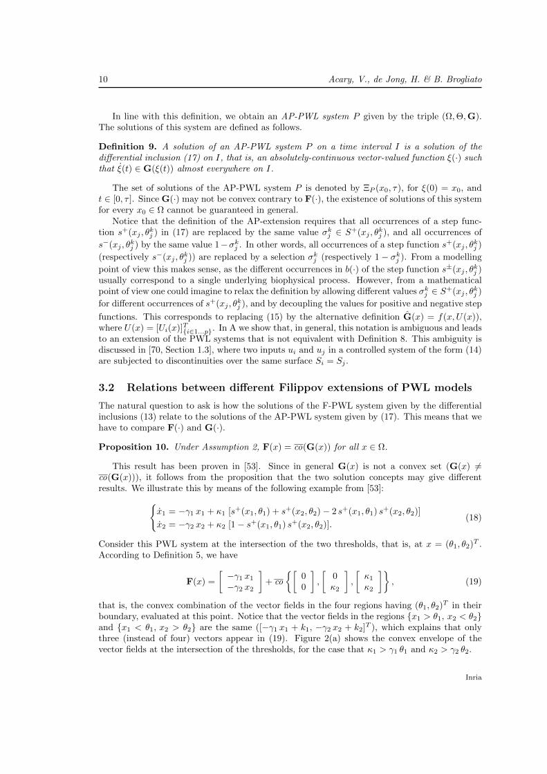
As can be seen in Figure 2(b), G(x) is not equal to F(x) at x = (θ1, θ2)T . The vertices of F(x)are included in G(x), where they correspond to the cases that σ1 and σ2 take their extremevalues 0 or 1, as shown in the figure. However, G(x) is a strict subset of F(x) and is not convex.
(a) (b)
Figure 2: The F- and AP-extensions of the PWL model (18) are different at x = (θ1, θ2)T ,the intersection point of the thresholds. (a) F(x), defined by (19), is the smallest closed convexset containing the vector fields of the four neighboring regions of x = (θ1, θ2)T , evaluated at theintersection point. (b) G(x) is obtained by varying the parameters σ1, σ2 over the interval [0, 1],as defined in (20). It includes the vector fields in the neighboring regions of x = (θ1, θ2)T , whichare obtained when σ1, σ2 take their extreme values 0 or 1. The plots are obtained for κ1 > γ1 θ1
and κ2 > γ2 θ2.
The example shows that the different Filippov extensions are not equivalent, but the questioncan be posed if differences occur when analyzing biologically relevant network structures. Forexample, the network represented by the PWL model (18) consists of two regulators that jointlyregulate their own genes, at exactly the same threshold concentrations, according to an XORswitch in the case of x1 and a NAND switch in the case of x2.1 A priori this is a rather unlikelyconfiguration to occur in real biological networks.
The following result shows that under Assumptions 2 and 4, which are usually not restrictivein practice, the different solution concepts proposed in the previous section coincide.
Proposition 11. Under Assumptions 2 and 4, F(x) = G(x) for all x ∈ Ω.
1The regulatory logic can be inferred by writing the equations in DNF. In the case of b1(x) = s+(x1, θ1) +s+(x2, θ2)− 2s+(x1, θ1) s+(x2, θ2) this yields s+(x1, θ1) s−(x2, θ2) + s−(x1, θ1) s+(x2, θ2), which corresponds toa Boolean XOR function. The function b2(x) = 1− s+(x1, θ1) s+(x2, θ2) is the algebraic equivalent of a BooleanNAND, that is, s−(x1, θ1) s−(x2, θ2) + s+(x1, θ1) s−(x2, θ2) + s−(x1, θ1) s+(x2, θ2).
RR n° 8207
12 Acary, V., de Jong, H. & B. Brogliato
Proof. We will prove the proposition by showing that G(x) = co(G(x)), so that the equality ofF(x) and G(x) directly follows from Prop. 10.
Following Definition 8, Gi(x) can be written in terms of gi(σ), with σ ∈ [0, 1]p and i ∈1, . . . , n. In what follows, it will be convenient to rewrite gi(σ) = gi(ρi), where ρi is thevector including all elements in σ appearing in bi(·), that is, those elements in σ occurring in theright-hand side of (17). Due to Assumption 4, ρi and ρj , i 6= j, have an empty intersection.
We now show by mathematical induction on the dimension k of ρi, k ≥ 1, that gi(ρi) is a closedinterval. For k = 1, it follows from Assumption 2 that gi(ρ
1i ) can be rewritten as a0
i + a1i ρ
1i ,
where a0i , a
1i ∈ R. Since ρ1
i ∈ [0, 1], ρ1i = 0, or ρ1
i = 1, gi(ρ1i ) is a closed interval. Suppose
that for some fixed k > 1, gi(ρ1i , . . . , ρ
ki ) is a closed interval (induction hypothesis). Then, by
Assumption 2, gi(ρ1i , . . . , ρ
k+1i ) can be rewritten as g0
i (ρ1i , . . . , ρ
ki ) + g1
i (ρ1i , . . . , ρ
ki ) ρk+1
i , for someg0i (·) and g1
i (·). From the induction hypothesis it follows that the expressions g0i (ρ1
i , . . . , ρki ) and
g1i (ρ1
i , . . . , ρki ) denote closed intervals, so with ρk+1
i ∈ [0, 1], ρk+1i = 0, or ρk+1
i = 1, we concludethat gi(ρ
1i , . . . , ρ
k+1i ) is a closed interval. This proves the assertion.
Due to Assumption 4 and the above, all gi(ρi) and therefore Gi(x) can be independentlyvaried, i ∈ 1, . . . , n. In other words, G(x) can be written as G1(x)× . . .×Gn(x) and is a closedhyperrectangle. As a consequence, G(x) is a closed convex set and G(x) = co(G(x)) = F(x)using Proposition 10.
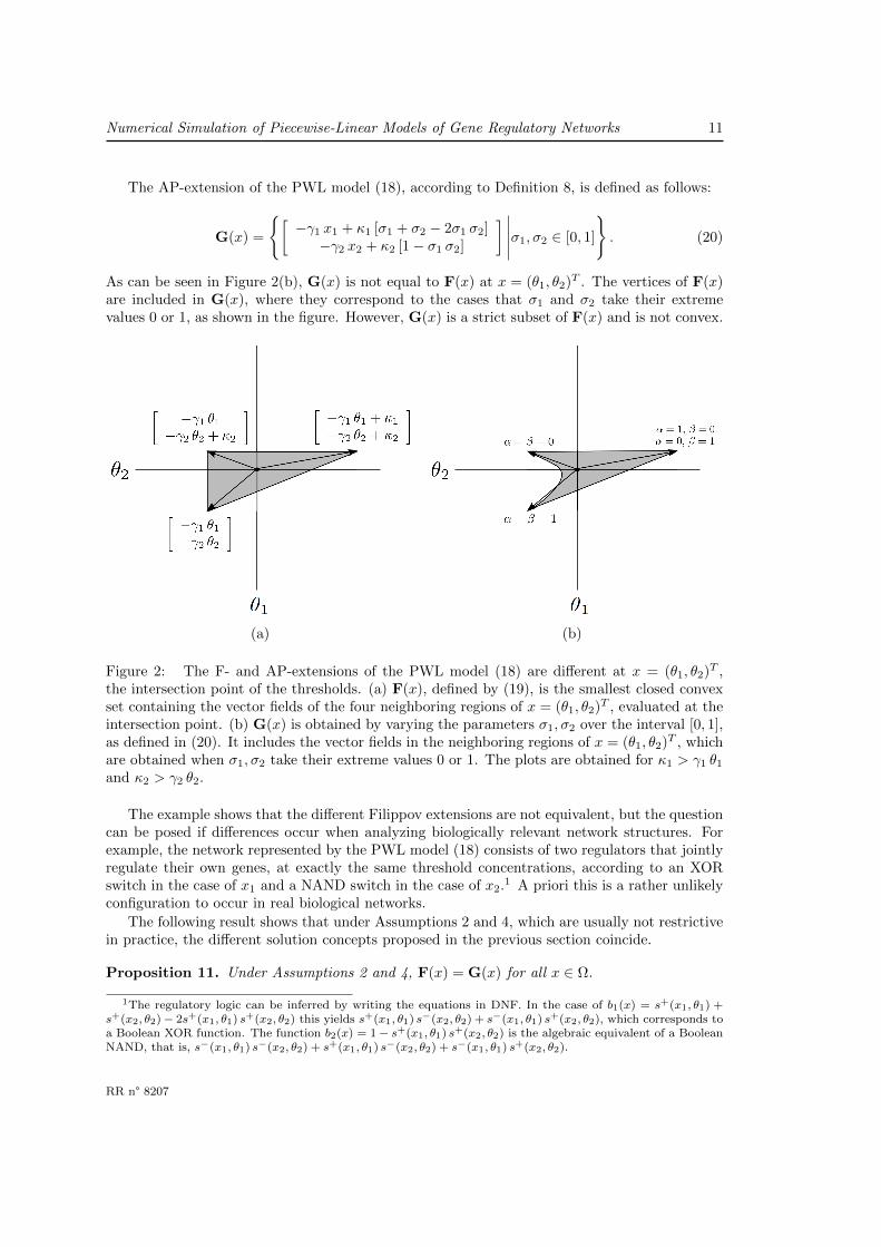
The PWL model of Figure 1 satisfies Assumptions 2 and 4, so that for this example thetwo Filippov extensions are equivalent. This can be illustrated for a point x on the segmentθ1
1 < x1 < θ21, x2 = θ2
2 (see Figure 3). A straightforward computation yields:
x ∈ F(x) =
[−γ1x1 + κ1
−γ2x2 + κ2σ2
] ∣∣∣∣∣σ2 ∈ [0, 1]
. (21)
By means of Definition 8, the same set is obtained for G(x).
Figure 3: Right-hand side of the Filippov differential inclusion (21) for the example network ofFigure 1, at x = (x1, x2)′ on the segment θ1
1 < x1 < θ21, x2 = θ2
2. In this example, F(x) andG(x) coincide.
As an aside, we notice that the following corollary holds, which makes explicit an intermediateresult in the proof of Prop. 11.
Corollary 12. Under Assumptions 2 and 4, F(x) and G(x) are hyperrectangular sets.
The qualitative analysis developed in [14, 26], and implemented in the computer tool GNA,exploits the mathematical properties of hyperrectangular overapproximations of the convex sets
Inria
Numerical Simulation of Piecewise-Linear Models of Gene Regulatory Networks 13
used in the classical Filippov approach. In particular, they facilitate the construction of discreteabstractions of the continuous dynamics, in the form of state transition graphs, in the absenceof precise quantitative information on the model parameters [14, 39]. The above corollary showsthat under reasonable and verifiable modeling assumptions, the results obtained are the sameas those obtained with the F- and AP-extensions of Definitions 5 and 8, respectively. In otherwords, under the assumptions of Prop. 11, the hyperrectangular sets are not overapproximationsbut exact.
While a qualitative analysis is appropriate for certain problems, the absence of precise quan-titative predictions is not desirable in others, such as the analysis of a limit cycle [1] or thedesign of a controller for a synthetic network [32]. The quantitative study of PWL models ofgene regulatory networks is hindered by the fact that, as of now, no general and efficient toolfor the numerical simulation of Filippov extensions is available. In the remainder of this paperwe show how tools developed for the simulation of nonsmooth mechanical, electrical and controlsystems [2, 3, 4, 5] can be adapted for this purpose.
4 Numerical methods for AP-extensions of PWL systems
In this section, we propose numerical methods for performing the time–integration of the AP-extension in Definition 8 and for computing its equilibrium points. General results of convergence(and existence) of solutions are beyond the scope of this paper, but we prove under the assumptionthat g(·) is continuous (satisfied under Assumption 2) that the discrete one–step problem isalways solvable. In practice, we can therefore always numerically compute a solution of thetime–discretized problem. In other words, this enables the computation of a selection in theset-valued AP-extension G(·) for the time–discrete system.
4.1 Reformulation of PWL models as Mixed Complementarity Sys-tems (MCS)
The main features of the proposed numerical time–integration method are the following:
1. A reformulation of the set–valued relation
σ ∈ S+(x, θ) (22)
in terms of well-known concepts from Convex Analysis and Optimization Theory (inclusioninto normal cones, Complementarity Problems (CP) and finite–dimensional VariationalInequalities (VI), see [34, 46]). One of the interests for introducing such concepts is theextensive amount of work that has been done for their mathematical analysis and theirnumerical treatment (see [34, 62] for an overview).
2. An implicit event-capturing time–stepping scheme, mainly based on the backward Eulerscheme, which allows to deal with the switch–like behaviour of the flow without resortingto an accurate detection of events. Furthermore, when a sliding motion occurs, such ascheme avoids the “chattering” effect when a attractive surface is reached [5].
3. The use of efficient numerical solvers for the one-step problem resulting from the time–discretization of the CP/VI formulation. At each time–step, we have to solve a CP (orequivalently a VI) for which numerous efficient solvers exist [16, 17, 29, 34, 36]. Efficientenumerative algorithms may also be used to list all possible solutions. When we are con-cerned with following a single solution trajectory, standard solvers for CP/VI succeed indoing this in an efficient way.
RR n° 8207
14 Acary, V., de Jong, H. & B. Brogliato
Let us start with the equivalent formulation of (22) as an inclusion in the normal cone to theinterval [0, 1]. We recall the definition of the normal cone to a convex set C at a point σ ∈ C:
NC(σ) = x | xT (σ′ − σ) ≤ 0 for all σ′ ∈ C. (23)
By noting that
N[0,1](σ) =
R− σ = 00, σ ∈ [0, 1]R+ σ = 1,
(24)
the relationσ ∈ S+(x, θ) (25)
can equivalently be reformulated as the following inclusion
(x− θ) ∈ N[0,1](σ). (26)
In turn, the relation (26) is equivalent to the complementarity conditions0 ≤ 1− σ ⊥ (x− θ)+ ≥ 00 ≤ σ ⊥ (x− θ)− ≥ 0,
(27)
where the symbol x ⊥ y means xT y = 0 and y+, y− stand for the positive and negative partsof y, respectively. Finally, an equivalent formulation of (26) is given by the following VI : findσ ∈ [0, 1] such that
(θ − x)T (σ − σ′) ≥ 0 for all σ′ ∈ [0, 1]. (28)
Let us define the notion of modes for the solution of the inclusion (26), or equivalently for theCP/VI formulations. Each solution is associated to a triplet of index sets
I+ = (j, k) ∈ 1 . . . n × 1 . . . pj | σkj = 1, xj − θkj ≥ 0I0 = (j, k) ∈ 1 . . . n × 1 . . . pj | σkj ∈ (−1, 1), xj − θkj = 0I− = (j, k) ∈ 1 . . . n × 1 . . . pj | σkj = −1, xj − θkj ≤ 0,
(29)
such that card(I+ ∪ I− ∪ I0) = p. A mode Mα ⊂ Ω× IRp, α ∈ 1 . . . 3p is defined by the set ofcouples (x, σ) such that the triplet of index-sets is equal to a given constant triplet of index sets.Since, in INp, there are 3p possibilities to choose these triplets, the total number of modes is 3p.
Let us now define the affine function y : Rn → Rp such that
y(x) = Cx− θ =
x1 − θ11
...x1 − θp11
...xn − θn1
...xn − θpn1
T
∈ Rp, (30)
where C ∈ Rp×n, with Cij ∈ 0, 1, and θ = [θ11, . . . , θ
p11 , . . . , θ1
n, . . . , θpnn ]T . Using the formulation
(26) and the definition of y(·), the AP-extension of the PWL system (17) in Definition 8 can bewritten compactly as
x = −diag(γ)x+ g(σ)
y(x) = Cx− θ ∈ N[0,1]p(σ)(31)
Inria
Numerical Simulation of Piecewise-Linear Models of Gene Regulatory Networks 15
where diag(γ) ∈ Rn×n is the diagonal matrix composed of γi, i ∈ 1 . . . n.When rewritten in the form (31), the system is a Mixed Complementarity System (MCS).
MCSs are an extension of Linear Complementarity Systems (LCS)[44] to the nonlinear case withnontrivial bounds on σ. LCS and MCS enter in the more general framework of DifferentialVariational Inequalities [57] where the solution set of a variational inequality comes into play inthe right–hand side of an ordinary differential equation. For more details on complementaritysystems and their relations with other types of nonsmooth dynamical systems, we refer to [4, 20,38].
Remark 13 (Equilibrium (stationary) points). Finding equilibrium points of the AP-extensionof PWL systems is equivalent to solving the following MCP
0 = −diag(γ)x+ g(σ)
y(x) = Cx− θ ∈ N[0,1]p(σ)(32)
or more compactlyCdiag(1/(1 + γ))g(σ)− θ ∈ N[0,1]p(σ). (33)
Using the fact that σ 7→ Cdiag(1/(1 + γ))g(σ) − θ is a continuous function and [0, 1]p isa compact convex set of Rp, the VI/CP (33) has a nonempty compact set of solutions (directapplication of Corollary 2.2.5 in [34, page 148]).
Equilibrium points can then be computed by solving the following problemCdiag(1/(1 + γ))g(σ)− θ ∈ N[0,1]p(σ)
x = diag(1/(1 + γ))g(σ)
x ∈ Rn+.(34)
4.2 The general time-discretization framework.
Numerical time–integration of an MCS (31) can be performed by two main families of solvers.The first one, often called event-detecting (or event-driven) time–stepping schemes, performs
an accurate location of the time of events. An event corresponds to a change of mode of solutionsas defined in the previous section. Between two events, any algorithm for Differential AlgebraicEquations (DAEs) can be used for the time integration of the smooth dynamics. In additionto the problem of the drift of constraints when the trajectory is sliding, which can render thedetection of events difficult, the main drawback of event-detecting schemes is the inability todeal with infinite accumulations of events in finite time (also termed as Zeno-phenomena). Inthe context of ordinary differential equations with a discontinuous right–hand side, an event-driven scheme for a class of piecewise–smooth systems reformulated as complementarity systemsis rigorously described in [65]. For an overview of event-driven schemes for nonsmooth systems,we refer to [4, Chapter 7].
The second family of schemes is the class of the event-capturing time–stepping schemes. Inthis case, no accurate detection of events is performed and the events may occur within thetime–step. Although these methods are of low order, they are robust, stable and enjoy someconvergence results under specified assumptions (see the survey paper [30] in the context ofgeneral differential inclusions). Moreover, they are able to deal with an infinite number of eventsin finite time, which is common in practice (see the example in Section 6.2).
For our specific class of inclusions, we are interested in developing a dedicated event-capturingtime–stepping scheme which takes benefits from the special structure of the complementaritysystems. As we said before, for such systems, the discretization results at each time–step in a
RR n° 8207
16 Acary, V., de Jong, H. & B. Brogliato
CP/VI for which there exists a large amount of efficient algorithms. Therefore, computing aselection of the right–hand side set–valued map of our time–discretization differential inclusioncan be done in a very efficient way. For general studies and a survey on time–stepping schemesfor complementarity systems, we refer to [6, 21, 43, 57] and [4, Chapter 9].
Let us now expose the proposed time discretization of (31) over a time–interval [tk, tk+1] oflength h:
xk+1 = xk − hdiag(γ)xk+τ + h g(σk+1)
yk+1 = Cxk+1 − θyk+1 ∈ N[0,1]p(σk+1),
(35)
with the initial condition x0 = x(t0). The notation xk+τ means τxk+1 + (1− τ)xk for τ ∈ [0, 1].The problem (35) is called the one-step problem that we have to solve on each interval. Let usdefine the vector
zk+1 =
[xk+1
σk+1
]∈ Rn+p, (36)
and the function F : Rn+p → Rn+p as
F (zk+1) =
[xk+1 − xk + hdiag(γ)xk+τ − h g(σk+1)
θ − Cxk+1
]. (37)
Then the problem (35) is equivalent to the following inclusion
−F (zk+1) ∈ NRn×[0,1]p(zk+1). (38)
Proposition 14. Let F : Rn+p → Rn+p be the function defined in (37). Under Assumption 2,the problem of finding z ∈ Rn × [0, 1]p such that
−F (z) ∈ NRn×[0,1]p(z) (39)
has a nonempty and compact solution set.
Proof. The proof is based on the application of Corollary 2.2.5 in [34, page 148] which statesthat the VI
y(σ)T (σ − σ′) ≥ 0, for all σ′ ∈ K ⊂ Rp, (40)
has a solution if K is compact convex, and y : K → Rp is continuous. The inclusion (38) can berestated as
x− xk + hdiag(γ)(τx+ (1− τ)xk)− h g(σk+1) = 0Cx− θ ∈ N[0,1]p(σ).
(41)
Since the matrix In + hτdiag(γ) is regular, we can solve the first equation for x. This yields thefollowing definition of y(·):
y(σ) = Cx− θ = C diag(1/(1 + hτγ)) [(In − h(1− τ) diag(γ))xk + h g(σ)]− θ, (42)
where diag(1/(1+hτγ)) is the diagonal matrix made of the components 1/(1+hτγi), i ∈ 1 . . . n.The inclusion in (41) becomes
y(σ) ∈ N[0,1]p(σ) (43)
and then is equivalent to (40). Since g is multiaffine, y is continuous. Choose K = [0, 1]p whichis compact convex. Then, the VI (40) has a nonempty and compact solution set for σ. Therelation
x = diag(1/(1 + hτγ)) [(In − h(1− τ) diag(γ))xk + h g(σ)] (44)
allows to build a nonempty and compact set of solutions for z = [x σ]T for (39).
Inria
Numerical Simulation of Piecewise-Linear Models of Gene Regulatory Networks 17
Remark 15. The following observations can be made :
• Proposition 14 is crucial for the success of the numerical scheme which is proposed in thispaper. It states that we can always find a solution of the discrete problem. It remains to bediscussed how to effectively compute one of these solutions.
• Only Assumption 2 is necessary to prove the result. It could even be relaxed to continuousfunctions g(·) instead of multiaffine.
• To avoid any misunderstanding, we have said nothing about the convergence of the schemeand we cannot straightforwardly extrapolate Proposition 14 for an existence result in contin-uous time. As explained above, F-extensions of PWL systems ensures existence of solutions.The AP-extension in general does not guarantee such a result.
At each step, we have to solve the so–called one–step problem which has been proved topossess solutions. In the sequel, we say a few words on the solution procedures in practise. Tothis end, let us now introduce a fairly standard problem in Mathematical Programming, whichis equivalent to the problem (35).
Definition 16 (Mixed Complementarity Problem(MCP) [29]). Given a function F : Rn+p →Rn+p and lower and upper bounds l, u ∈ Rn+p∪−∞,+∞, the Mixed Complementarity Problem(MCP) is to find z ∈ Rn+p and w, v ∈ Rn+p
+ such thatF (z) = w − vl ≤ z ≤ u
(u− z)T v = 0(z − l)Tw = 0.
(45)
By choosing l ∈ −∞n × 0p and u ∈ +∞n × 1p, solving the inclusion (38) is equivalentto solve an MCP for zk+1 where the vectors wk+1, vk+1 ∈ Rn+p are of the form
(wk+1)i =
0, 1 ≤ i ≤ n(y−k+1)i−n, n ≤ i ≤ n+m
, (vk+1)i =
0, 1 ≤ i ≤ n(y+k+1)i−n, n ≤ i ≤ n+m
. (46)
Numerical algorithms for solving such problems benefit from a long experience (see [16, 29] forthe PATH solver and [17] for a comprehensive comparison of algorithms).
4.3 An enumerative procedure based on the Newton–Josephy approach
In most of the applications, the numerical algorithms cited in the previous section are sufficientfor computing a solution of the one–step problem. Nevertheless, it can be interesting to be ableto enumerate the solutions when they are multiple and isolated. To this end, we can benefitfrom the fact that y(·) is a linear function of its arguments and g(·) is a multiaffine applicationfor easily applying a Newton–like method. For solving the one-step problem (38) in its MCPformulation, the Newton–Josephy method [48, 63] is used which consists in a linearization of thefirst line of the time–discretization (35). Then, the MCP is solved by a sequential Mixed LinearComplementarity Problem (MCLP) method using a dedicated enumerative solver for MLCP.
Let us introduce the following nonlinear residue
R(x, σ) = (In + τhdiag(γ))x− (In − h(1− τ)diag(γ))xk − h g(σ). (47)
RR n° 8207
18 Acary, V., de Jong, H. & B. Brogliato
The solutions xk+1 and σk+1 of (38) satisfy R(xk+1, σk+1) = 0. The solutions of the nonlinearsystem (47) are sought as the limit of the sequence xν , σνν∈N verifying
RL(xν+1, σν+1) = 0x0 = xk, σ
0 = σk,
where the Newton linearization of R is given by
RL(xν+1, σν+1) = R(xν , σν) +∇xR(xν , σν)(xν+1 − xν) +∇σR(xν , σν)(σν+1 − σν).
Let us introduce the so-called iteration matricesM = ∇xR(x, σ) = In + hτdiag(γ)B(σ) = ∇σR(x, σ) = ∇σg(σ).
At each time-step k, we have to solve the following linearized problem
xν+1 =M−1[(In − h(1− τ)diag(γ))xk + hg(σν) + hB(σν)(σν+1 − σα)
]. (48)
Inserting into (48) the definition of y(·) given by (30), we get the following linear relationbetween yν+1 and σν+1
yν+1 =CM−1[(In − h(1− τ)diag(γ))xk + hg(σν) + hB(σν)(σν+1 − σν)
]− θ.
To summarize, the problem to be solved at each Newton iteration isyν+1 = W ν+1σν+1 + qν+1
yν+1 ∈ N[0,1]p(σν+1),(49)
where W ∈ Rp×p and q ∈ Rp are defined as
W ν+1 = hCM−1B(σν)
qν+1 = CM−1 [(In − h(1− τ)diag(γ))xk + hg(σν) + hB(σν)σν ]− θ.
The problem (49) is an MLCP which can be solved under suitable assumptions by many lin-ear complementarity solvers such as pivoting techniques, interior point techniques and split-ting/projection strategies [25]. Among these techniques, some efficient enumerative solvers canalso be used (see for instance [10, 49, 64]), if we are interested in enumerating several solu-tions corresponding to various modes of the switching functions. This approach has thereforean interest from the qualitative point of view since it allows to outline multiple solutions and tochoose following one particular solution in the numerical time integration. This feature will beillustrated in the oscillator example of Section 6.2.
4.4 Software aspects
The simulation platform Siconos2 developed at INRIA [3, 4, 8] implements the numerical meth-ods for AP extensions of PWL models described in the previous section. The Siconos platformis an open–source software for the modeling, simulation, analysis and control of nonsmooth dy-namical systems. It has been designed and developed with a constant effort to be sufficientlygeneral and modular to be able to deal with applications ranging over several domains, including,Mechanics, Electronics, Control, Systems Theory (see the Siconos website for examples).
2http://siconos.gforge.inria.fr
Inria
Numerical Simulation of Piecewise-Linear Models of Gene Regulatory Networks 19
In the following, we use the Siconos platform for the simulation of gene regulatory networks.In order to achieve this, the following general formulation of MCS is usedMx = f(x, t) + g(x, t, λ)
y = h(x, t, λ)−y ∈ N[l,u](λ)
(50)
where M is a non–necessarily regular matrix and f(·), g(·) and h(·) are assumed to be user-defined smooth functions. Without any optimization for to the special case of AP-extensionsgiven by (31), the computation time for each trajectory is between 15 ms and 1 s on a laptopcomputer (Apple MacBook Pro 3.60GHz Intel Core 2 Duo). All examples presented in the nextsection are included in the collection of examples distributed with Siconos.
5 Illustration of the properties of the numerical methodson a two-gene regulatory network
This section is devoted to the presentation of the properties of the above numerical methods onthe genetic regulatory network of two genes in Figure 1, modeled by the two-dimensional system:
x1 = −γ1 x1 + κ1 s+(x2, θ
12) s−(x1, θ
21)
x2 = −γ2 x2 + κ2 s+(x1, θ
11) s−(x2, θ
22),
(4)
with the following parameters: θ11 = θ1
2 = 4, θ21 = θ2
2 = 8, κ1 = κ2 = 40, γ1 = 4.5 and γ2 = 1.5.In particular, we detail the MCS formulation and we propose an analysis in a subset of Ω whereall surfaces are attractive. We show that the proposed formulation enables one to show theuniqueness of the solution of the one–step problem and the finite–time stability of one of theequilibrium points.
5.1 MCS formulation and stability analysis
We have card(L) = 2, n = 2 and p = 4. Let y(x) =[x1 − θ1
1, x1 − θ21, x2 − θ1
2, x2 − θ22
]Tand
σ ∈ R4. We also have
g(σ) =
[κ1σ
12(1− σ2
1)κ2σ
11(1− σ2
2)
], B(σ) =
[0 −κ1σ
12 κ1(1− σ2
1) 0κ2(1− σ2
2) 0 0 −κ2σ11
],
M = I2 + hτ
[γ1 00 γ2
], C =
1 01 00 10 1
. (51)
There are three equilibrium points, two of which are attractive ((0, 0) and (θ21, θ
22)) and a third
one repulsive ((θ11, θ
12)). We focus on the equilibrium point x1 = θ2
1 and x2 = θ22 by restricting
the domain of interest to Ω = Ω ∩ (θ11,+∞) × (θ2
1,+∞). In Ω, we have σ11 = 1 since x1 > θ1
1,and σ1
2 = 1 since x2 > θ12, so that the original system (31) can be reduced to
x = −diag(γ)x+ Bσ + κ
Cx− θ ∈ N[0,1]2(σ),(52)
with
σ =
[σ2
1
σ22
], C =
[1 00 1
], θ =
[θ2
1
θ22
], B =
[−κ1 0
0 −κ2
], κ =
[κ1
κ2
]. (53)
RR n° 8207
20 Acary, V., de Jong, H. & B. Brogliato
The complementarity systems (or equivalently, differential variational inequalities) frameworkprovides not only an efficient framework for simulation, but it can also help us to conclude onthe stability, possibly in finite–time, of the equilibrium point (θ2
1, θ22) in Ω. On one hand, the
study of the stability of PWL systems for gene regulatory networks has already been studiedin [23], while on the other hand there is a huge literature dealing with the stability of Filippovsystems and differential inclusions, and in particular of the finite–time stability [56]. We do notwish to give an exhaustive treatment of the stability of PWL systems by means of monotonedifferential inclusions, which is beyond the scope of the paper. The following result, however,gives an idea of the large range of applicability of the complementarity systems techniques.
Lemma 17. The equilibrium point θ = (θ21, θ
22)T is finite-time stable in Ω.
Proof. Since −B is a symmetric definite positive matrix, we choose a symmetric positive definitematrix R as a square root of the inverse of B, i.e. R2 = −B−1. Following [19], let us performthe state transformation z = R(x− θ). The solution of the reduced system (52) is equivalent tothe following inclusion
−z ∈ T (z), (54)
with the multi-valued operator T defined as
T (z) = R diag(γ)R−1z+, (diag(γ)θ − κ) +R−1S+(R−1z, 0). (55)
Since S+(·, 0) is monotone and R = RT , R−1S+(R−1 ·, 0) is also monotone [62, Exercice 12.4].Since R is a diagonal matrix, we have R diag(γ)R−1 = diag(γ) which obviously is a positivedefinite matrix. As a consequence, the operator T (·) is a strongly monotone mapping in Ω, i.e.,there exists c > 0
(λ′ − λ)T (x− y) ≥ c‖x− y‖2, ∀x, y ∈ Ω, ∀λ′ ∈ T (x),∀λ ∈ T (y). (56)
Let us compute the set T (0)
T (0) = −diag(γ)θ + κ+ BS+(θ, θ) = [−36, 4]× [−12, 28]. (57)
The existence of an equilibrium point for x = θ is ensured by 0 ∈ T (0). Choosing a Lyapunovfunction V (z) = 1/2z2, we have V (0) = 0, V (z) ≥ 0 for all z and
V (z) = zT z with − z ∈ T (z). (58)
Since T (·) is strongly monotone and 0 ∈ T (0), we can conclude that V (z) ≤ c‖z‖2, c > 0 andthat the equilibrium point is exponentially stable. To prove the finite–time stability, we use thefact that T (·) is simply monotone,
(λ′ − λ)T (x− y) ≥ 0, ∀x, y ∈ Ω, ∀λ′ ∈ T (x),∀λ ∈ T (y). (59)
in conjunction with the fact that there exists a ball of radius r ∈ (0, 4) included in T (0):
Br(0) = z | ‖z‖ ≤ r ⊂ T (0). (60)
For −λ ∈ T (z) and −λ0 ∈ T (0), we get
(λ− λ0)T z ≤ 0. (61)
Choosing z 6= 0 and −λ0 = −rz/‖z‖ ∈ Br(0)) ⊂ T (0), we have
λT z ≤ r zT
‖z‖z = r‖z‖. (62)
Inria
Numerical Simulation of Piecewise-Linear Models of Gene Regulatory Networks 21
Since −λ ∈ T (z), we get for z 6= 0,
V (z) + r√|V (z)| ≤ 0. (63)
Assume for any t1 > t0 that V (z(t1)) > 0. Then we can divide (63) by√|V (z)| and perform a
time integration between t1 and t0√|V (z(t1))| −
√|V (z(t0))| ≤ −r(t1 − t0). (64)
From (64), we infer that limt1→+∞ V (z(t1)) = −∞. By contradiction, we can conclude thatthere exists a finite time t1 such that V (z(t1)) = 0. In other words, the equilibrium z = 0 isreached in finite time.
In the following section, we are interested in the discrete–time properties of the numericalscheme.
5.2 Properties of the numerical simulations
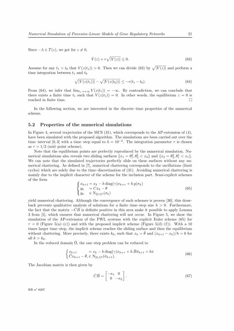
In Figure 4, several trajectories of the MCS (31), which corresponds to the AP-extension of (4),have been simulated with the proposed algorithm. The simulations are been carried out over thetime–interval [0, 3] with a time–step equal to h = 10−2. The integration parameter τ is chosenas τ = 1/2 (mid–point scheme).
Note that the equilibrium points are perfectly reproduced by the numerical simulation. Nu-merical simulations also reveals two sliding surfaces x1 = θ2
1, θ12 < x2 and x2 = θ2
2, θ11 < x1.
We can note that the simulated trajectories perfectly slide on these surfaces without any nu-merical chattering. As defined in [7], numerical chattering corresponds to the oscillations (limitcycles) which are solely due to the time–discretization of (31). Avoiding numerical chattering ismainly due to the implicit character of the scheme for the inclusion part. Semi-explicit schemesof the form xk+1 = xk − hdiag(γ)xk+τ + h g(σk)
yk = Cxk − θyk ∈ N[0,1]p(σk)
(65)
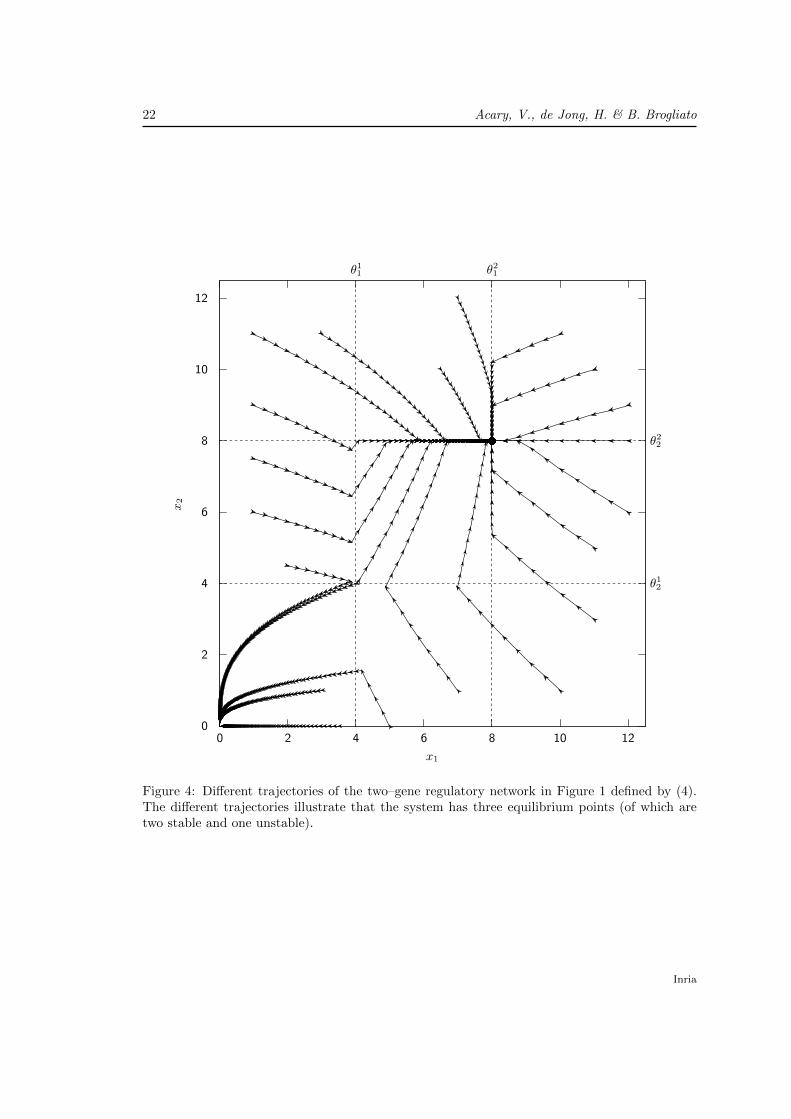
yield numerical chattering. Although the convergence of such schemes is proven [30], this draw-back prevents qualitative analysis of solutions for a finite time–step size h > 0. Furthermore,the fact that the matrix −CB is definite positive in this area make it possible to apply Lemma3 from [5], which ensures that numerical chattering will not occur. In Figure 5, we show thesimulation of the AP-extension of the PWL systems with the explicit Euler scheme (65) forτ = 0 (Figure 5(a)–(c)) and with the proposed implicit scheme (Figure 5(d)–(f)). With a 10times larger time–step, the implicit scheme reaches the sliding surface and then the equilibriumwithout chattering. More precisely, there exists k0, such that xk = θ and (xk+1 − xk)/h = 0 forall k > k0.
In the reduced domain Ω, the one–step problem can be reduced toxk+1 = xk − hdiag(γ)xk+τ + h Bσk+1 + hκCxk+1 − θ,∈ N[0,1]2(σk+1).
(66)
The Jacobian matrix is then given by
CB =
[−κ1 0
0 −κ2
]. (67)
RR n° 8207
22 Acary, V., de Jong, H. & B. Brogliato
0
2
4
6
8
10
12
0 2 4 6 8 10 12
x2
x1
θ12
θ22
θ11 θ21
Figure 4: Different trajectories of the two–gene regulatory network in Figure 1 defined by (4).The different trajectories illustrate that the system has three equilibrium points (of which aretwo stable and one unstable).
Inria
Numerical Simulation of Piecewise-Linear Models of Gene Regulatory Networks 23
Since κi > 0, the matrix −CB is definite positive in Ω and we have
−xT CBx ≥ κ‖x‖2 (68)
with κ = min(κ1, κ2). This means that the VI
θ − Cdiag(1/(1 + hτγ))[(In − h(1− τ) diag(γ))xk + h Bσ + hκ)
]∈ N[0,1]2(σ) (69)
is strongly monotone and has a unique solution (see [34, Theorem 2.3.3]), given by
(σ21)k+1 = proj[0,1]
(1 + hτγ1
hκ1
[θ2
1 −1
1 + hγ1(1− h(1− τ)γ1x1,k+1 + hκ1)
])(σ2
2)k+1 = proj[0,1]
(1 + hτγ2
hκ2
[θ2
2 −1
1 + hγ2(1− h(1− τ)γ2x2,k+1 + hκ2)
]).
(70)
5
6
7
8
9
10
5 6 7 8 9 10
x2
x1
θ22
θ21
(a)
6.4
6.6
6.8
7
7.2
7.4
7.6
7.8
8
8.2
7.9 8 8.1 8.2 8.3 8.4 8.5
x2
x1
θ22
θ21
(b)
7.95
7.96
7.97
7.98
7.99
8
8.01
7.985 7.99 7.995 8 8.005 8.01 8.015 8.02 8.025
x2
x1
θ22
θ21
(c)
5
6
7
8
9
10
5 6 7 8 9 10
x2
x1
θ22
θ21
(d)
6.4
6.6
6.8
7
7.2
7.4
7.6
7.8
8
8.2
7.9 8 8.1 8.2 8.3 8.4 8.5
x2
x1
θ22
θ21
(e)
7.95
7.96
7.97
7.98
7.99
8
8.01
7.985 7.99 7.995 8 8.005 8.01 8.015 8.02 8.025
x2
x1
θ22
θ21
(f)
Figure 5: Illustration of the numerical chattering effect by zooming in on the state space on thesystem (4) as shown in Figure 4. The trajectories start from x(t0) = [10, 5]T . (a)–(c). Differentzooms on the trajectory obtained with the explicit Euler scheme (h = 10−3). (d)–(f). Differentzooms on the trajectory obtained with the proposed implicit Euler scheme (h = 10−2).
To conclude this first example, the MCS formulation with an implicit time–discretizationallows us to reproduce the main features of the dynamics of the PWL models of the gene reg-
RR n° 8207
24 Acary, V., de Jong, H. & B. Brogliato
ulatory network: equilibrium points, sliding surfaces, finite–time stability. In the next section,some more realistic examples are considered.
6 Applications in synthetic biology
In this section we apply the simulation methods developed above to the analysis of actual bio-logical networks. We consider three examples from the field of synthetic biology [51], which allconcern relatively small networks that have been designed from pre-existing, well-characterizedmolecular elements and implemented in the cell to perform a particular function. The first twonetworks have been shown able to exhibit oscillations ([12, 33], see [61] for a review on syn-thetic oscillators). The third network is capable of a variety of dynamic behaviors and has beenproposed as a benchmark for the reverse engineering of the network structure from time-coursedata [22]. In the three cases we transformed the network structure into PWL equations, takinginspiration from existing ODE models, and we compared the dynamic features of the networksrevealed by the simulations with available experimental data.
For each of the networks described above, we determined the equilibrium points and numer-ically computed solutions exemplifying the dynamics of the PWL systems. The mathematicalanalysis of equilibrium points of PWL models (1) was based on analytical results in the litera-ture, concerning both equilibrium points within regions separated by threshold planes (x 6∈ Θ)and equilibrium points located on one or several threshold planes (x ∈ Θ) [23, 39, 58]. Whilethe former are always asymptotically stable in the classical sense [39], analyzing the stabilityof the latter requires generalized definitions adapted to the non-uniqueness of solutions of PWLsystems. In particular, we used the results developed in [23] for F-extensions of PWL models(Definition 5), which provide easy-to-verify criteria for checking the stability in a number oftypical cases. Notice that in the examples below, Assumptions 2 and 4 are always satisfied,which means that the F-extensions used for stability analysis and the AP-extensions used forsimulation are equivalent (Proposition 11). As a consequence, the results obtained for the threeexample networks are valid for the different solution concepts reviewed in Section 3.
6.1 Repressilator
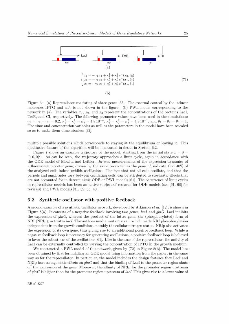
A repressilator is a network of several genes with a cyclic structure. Each gene codes for atranscription regulator that represses the next gene in the cycle. Elowitz and Leibler [33] haveimplemented a repressilator in the model bacterium E. coli, using the genes lacI, tetR, and cI(Figure 6(a)). The network can be externally controlled by adding the small inducer moleculesIPTG and aTc to the growth medium, which inactivate LacI and TetR, respectively. Startingfrom their ODE model, we formulated a PWL model of the three-gene repressilator. The majorchange consists in lumping transcription and translation into a single step and replacing thesigmoidal regulation functions by step functions. The parameter values in [33] have been adaptedaccordingly (see Figure 6(b)).
The PWL model of the repressilator has a single equilibrium point, in accordance with theODE model of Elowitz and Leibler. This equilibrium point is located at the intersection ofthe three thresholds, that is, at x = θ = [θ1, θ2, θ3]T . The equilibrium point is thus also adiscontinuity point of the PWL model. More precisely, the set of solutions starting from x = θincludes solutions that remain at the equilibrium point as well as solutions that leave this pointat any time t ≥ 0. For the chosen parameter values, the equilibrium point is therefore unstable[23]. The numerical solver finds an infinite number of solutions starting from x = θ. At eachtime–step, starting from the equilibrium point x = θ, an enumerative MCP solver is able to list
Inria
Numerical Simulation of Piecewise-Linear Models of Gene Regulatory Networks 25
LacI
lacI
TetR
tetR cI
CI
(a)x1 = −γ1 x1 + κ1
1 + κ21 s
−(x3, θ3)x2 = −γ2 x2 + κ1
2 + κ22 s
−(x1, θ1)x3 = −γ3 x3 + κ1
3 + κ23 s
−(x2, θ2)(71)
(b)
Figure 6: (a) Repressilator consisting of three genes [33]. The external control by the inducermolecules IPTG and aTc is not shown in the figure. (b) PWL model corresponding to thenetwork in (a). The variables x1, x2, and x3 represent the concentrations of the proteins LacI,TetR, and CI, respectively. The following parameter values have been used in the simulations:γ1 = γ2 = γ3 = 0.2, κ1
1 = κ12 = κ1
3 = 4.8 10−4, κ21 = κ2
2 = κ23 = 4.8 10−1, and θ1 = θ2 = θ3 = 1.
The time and concentration variables as well as the parameters in the model have been rescaledso as to make them dimensionless [33].
multiple possible solutions which corresponds to staying at the equilibrium or leaving it. Thisqualitative feature of the algorithm will be illustrated in detail in Section 6.2.
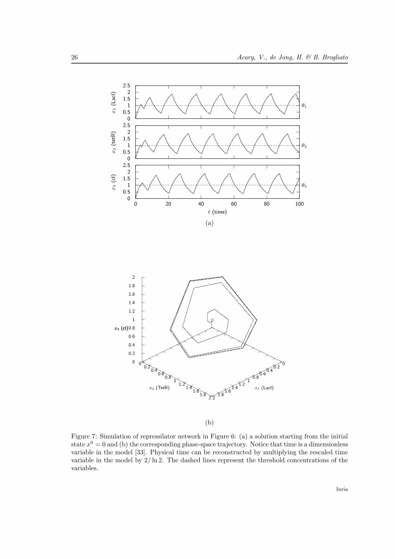
Figure 7 shows an example trajectory of the model, starting from the initial state x = 0 =[0, 0, 0]T . As can be seen, the trajectory approaches a limit cycle, again in accordance withthe ODE model of Elowitz and Leibler. In-vivo measurements of the expression dynamics ofa fluorescent reporter gene, driven by the same promoter as the gene cI, indicate that 40% ofthe analyzed cells indeed exhibit oscillations. The fact that not all cells oscillate, and that theperiods and amplitudes vary between oscillating cells, can be attributed to stochastic effects thatare not accounted for in deterministic ODE or PWL models [61]. The occurrence of limit cyclesin repressilator models has been an active subject of research for ODE models (see [61, 68] forreviews) and PWL models [31, 32, 35, 40].
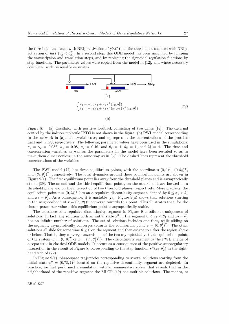
6.2 Synthetic oscillator with positive feedback
A second example of a synthetic oscillator network, developed by Atkinson et al. [12], is shown inFigure 8(a). It consists of a negative feedback involving two genes, lacI and glnG : LacI inhibitsthe expression of glnG, whereas the product of the latter gene, the (phosphorylated) form ofNRI (NRIp), activates lacI. The authors used a mutant strain which made NRI phosphorylationindependent from the growth conditions, notably the cellular nitrogen status. NRIp also activatesthe expression of its own gene, thus giving rise to an additional positive feedback loop. While anegative feedback loop is necessary for generating oscillations, a positive feedback loop is believedto favor the robustness of the oscillations [61]. Like in the case of the repressilator, the activity ofLacI can be externally controlled by varying the concentration of IPTG in the growth medium.
We constructed a PWL model of this network, given by (72) in Figure 8(b). The model hasbeen obtained by first formulating an ODE model using information from the paper, in the sameway as for the repressilator. In particular, the model includes the design features that LacI andNRIp have antagonistic effects on glnG and that the binding of LacI to the promoter region shutsoff the expression of the gene. Moreover, the affinity of NRIp for the promoter region upstreamof glnG is higher than for the promoter region upstream of lacI. This gives rise to a lower value of
RR n° 8207
26 Acary, V., de Jong, H. & B. Brogliato
00.5
11.5
22.5
x1
(Lac
I)θ1
00.5
11.5
22.5
x2
(tet
R)
θ2
00.5
11.5
22.5
0 20 40 60 80 100
x3
(cI)
t (time)
θ3
(a)
00.2
0.40.6
0.81
1.21.4
1.61.8
2
00.2
0.40.6
0.81
1.21.4
1.61.8
2
0
0.2
0.4
0.6
0.8
1
1.2
1.4
1.6
1.8
2
x3 (cI)
x1 (LacI)x2 (TetR)
x3 (cI)
(b)
Figure 7: Simulation of repressilator network in Figure 6: (a) a solution starting from the initialstate x0 = 0 and (b) the corresponding phase-space trajectory. Notice that time is a dimensionlessvariable in the model [33]. Physical time can be reconstructed by multiplying the rescaled timevariable in the model by 2/ ln 2. The dashed lines represent the threshold concentrations of thevariables.
Inria
Numerical Simulation of Piecewise-Linear Models of Gene Regulatory Networks 27
the threshold associated with NRIp-activation of glnG than the threshold associated with NRIp-activation of lacI (θ1
2 < θ22). In a second step, this ODE model has been simplified by lumping
the transcription and translation steps, and by replacing the sigmoidal regulation functions bystep functions. The parameter values were copied from the model in [12], and where necessarycompleted with reasonable estimates.
LacI
lacI
NRI
glnG
NRIp
(a)x1 = −γ1 x1 + κ1 s
+(x2, θ22)
x2 = −γ2 x2 + κ2 s−(x1, θ1) s
+(x2, θ12)
(72)
(b)
Figure 8: (a) Oscillator with positive feedback consisting of two genes [12]. The externalcontrol by the inducer molecule IPTG is not shown in the figure. (b) PWL model correspondingto the network in (a). The variables x1 and x2 represent the concentrations of the proteinsLacI and GlnG, respectively. The following parameter values have been used in the simulations:γ1 = γ2 = 0.032, κ1 = 0.08, κ2 = 0.16, and θ1 = 1, θ1
2 = 1, and θ22 = 4. The time and
concentration variables as well as the parameters in the model have been rescaled so as tomake them dimensionless, in the same way as in [33]. The dashed lines represent the thresholdconcentrations of the variables.
The PWL model (72) has three equilibrium points, with the coordinates (0, 0)T , (0, θ12)T ,
and (θ1, θ22)T , respectively. The local dynamics around these equilibrium points are shown in
Figure 9(a). The first equilibrium point lies away from the threshold planes and is asymptoticallystable [39]. The second and the third equilibrium points, on the other hand, are located on athreshold plane and on the intersection of two threshold planes, respectively. More precisely, theequilibrium point x = (0, θ1
2)T lies on a repulsive discontinuity segment, defined by 0 ≤ x1 < θ1
and x2 = θ12. As a consequence, it is unstable [23]. Figure 9(a) shows that solutions starting
in the neighborhood of x = (θ1, θ22)T converge towards this point. This illustrates that, for the
chosen parameter values, this equilibrium point is asymptotically stable.
The existence of a repulsive discontinuity segment in Figure 9 entails non-uniqueness ofsolutions. In fact, any solution with an initial state x0 in the segment 0 < x1 < θ1 and x2 = θ1
2
has an infinite number of solutions. The set of solutions includes one that, while sliding onthe segment, asymptotically converges towards the equilibrium point x = (0, θ1
2)T . The othersolutions all slide for some time ℵ ≥ 0 on the segment and then escape to either the region aboveor below. That is, they converge towards one of the two asymptotically stable equilibrium pointsof the system, x = (0, 0)T or x = (θ1, θ
22)T ). The discontinuity segment is the PWL analog of
a separatrix in classical ODE models. It occurs as a consequence of the positive autoregulatoryinteraction in the circuit of Figure 8, corresponding to the step function s+(x2, θ
12) in the right-
hand side of (72).
In Figure 9(a), phase-space trajectories corresponding to several solutions starting from theinitial state x0 = (0.78, 1)T located on the repulsive discontinuity segment are depicted. Inpractice, we first performed a simulation with an enumerative solver that reveals that in theneighborhood of the repulsive segment the MLCP (49) has multiple solutions. The modes, as
RR n° 8207
28 Acary, V., de Jong, H. & B. Brogliato
defined in Section 4, are recorded. Once this first simulation has been performed, the user canchoose a preferred solution (encoded by one triplet of index sets) on a user–supplied part of thetrajectory, by asking the numerical solver to check if a solution with the given triplet exists.For the trajectories shown in Figure 9(a), three possible solutions have been detected in theneighborhood of the repulsive segment. A new simulation has been performed asking to preferthe triplet corresponding to the solution that slides on the segment. For the other trajectories,we changed the preferred solution when the trajectory reaches x1 = 0.55 and x1 = 0.4 to thetriplet of solutions that yields a trajectory escaping below and above, respectively.
Atkinson et al. [12] measured the time-varying dynamics of the circuit on the populationlevel using the chromosomal lacZ gene. This gene is under the control of LacI and encodesβ-galactosidase, whose levels can be assayed. The authors observed damped oscillations of β-galactosidase, which corresponds to the dynamics of the PWL model when the initial LacIconcentration lies above its first threshold (x0
1 > θ11, see Figure 9). In order to verify that damped
oscillations on the population level are not due to the desynchronization of individual cells thateach exhibit stable oscillations, Atkinson et al. [12] also measured gene expression in single cells,using a fluorescent reporter gene fused to a LacI-repressible promoter. The results confirm theoccurrence of damped oscillations in the oscillator with positive feedback, in agreement with thepopulation-level assay.
6.3 IRMA: a synthetic benchmark network
IRMA is a synthetic network constructed in yeast and proposed as a benchmark for modelingand identification approaches [22]. The network consists of five well-characterized genes thathave been chosen so as to include different kinds of interactions, notably transcription regulationand protein-protein interactions. The structure of the IRMA network is shown in Figure 10(a).The expression of the CBF1 gene is positively regulated by Swi5 and negatively regulated byAsh1. CBF1 encodes the transcription factor Cbf1 that activates expression of the GAL4 gene.The expression of SWI5 is activated by Gal4, but only in the absence of Gal80 or in the presenceof galactose. Gal80 binds to the Gal4 activation domain, but galactose releases this inhibition oftranscription. The product of SWI5 activates the expression of three other genes in the network:ASH1, CBF1, and GAL80. The network contains one positive and two negative feedback loops.Consequently, for suitable parameter values IRMA might function as a synthetic oscillator [54].
Figure 10(b) shows a PWL model of IRMA that was previously developed [15]. The regulatoryfunctions in the model encode the interaction structure described above. Most parameters valuesin the PWL model were taken from the original IRMA publication. In a few cases, however,they were slightly adapted to satisfy inequality constraints between parameters that were inferredfrom the experimental data [15].
Using the model (73), we simulated the behavior of the network in response to two differentperturbations: shifting cells from glucose to galactose medium (switch-on experiments), and fromgalactose to glucose medium (switch-off experiments). The terms switch-on (switch-off) refer tothe activation (inhibition) of SWI5 expression during growth on galactose (glucose). For thesetwo perturbations, the temporal evolution of the expression of all the genes in the network wasmonitored by qRT-PCR with good time resolution in [22].
In switch-off conditions, when s+(u, θu) = 1, the PWL system has a single asymptoticallystable equilibrium point, not located on a threshold plane. At this equilibrium point all genesare expressed at their basal level x = (κ1
1/γ1, κ12/γ2, κ
13/γ3, 0, κ
15/γ5)T . The measured time-series
expression profiles of the five network genes in a switch-off experiments indeed show that thesystem evolves towards a basal state [22].
In switch-on conditions, when s+(u, θu) = 0, the PWL system has three equilibrium points.
Inria
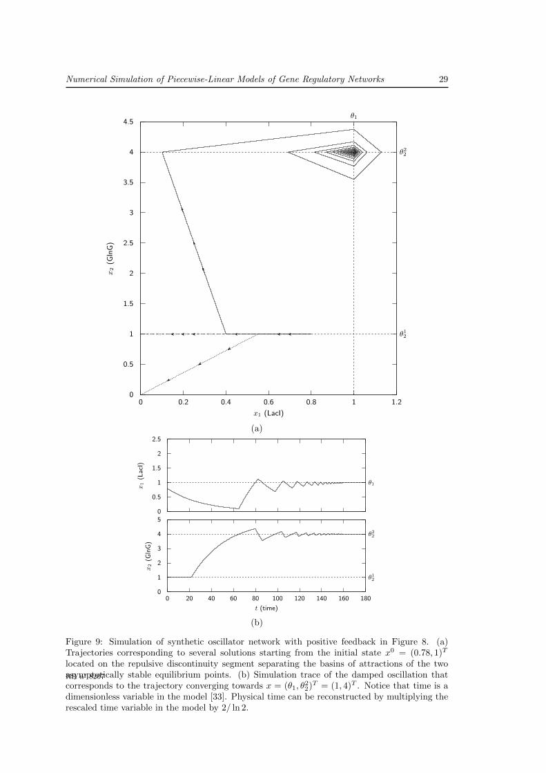
Numerical Simulation of Piecewise-Linear Models of Gene Regulatory Networks 29
0
0.5
1
1.5
2
2.5
3
3.5
4
4.5
0 0.2 0.4 0.6 0.8 1 1.2
x2
(Gln
G)
x1 (LacI)
θ12
θ22
θ1
(a)
0
0.5
1
1.5
2
2.5
x1
(Lac
I)
θ1
0
1
2
3
4
5
0 20 40 60 80 100 120 140 160 180
x2
(Gln
G)
t (time)
θ12
θ22
(b)
Figure 9: Simulation of synthetic oscillator network with positive feedback in Figure 8. (a)Trajectories corresponding to several solutions starting from the initial state x0 = (0.78, 1)T
located on the repulsive discontinuity segment separating the basins of attractions of the twoasymptotically stable equilibrium points. (b) Simulation trace of the damped oscillation thatcorresponds to the trajectory converging towards x = (θ1, θ
22)T = (1, 4)T . Notice that time is a
dimensionless variable in the model [33]. Physical time can be reconstructed by multiplying therescaled time variable in the model by 2/ ln 2.
RR n° 8207
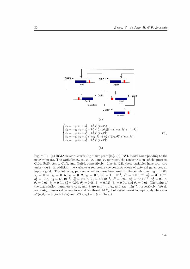
30 Acary, V., de Jong, H. & B. Brogliato
Gal4
GAL4
Swi5
SWI5
Gal80
GAL80
ASH1CBF1
ASH1CBF1
Galactose
(a)x1 = −γ1 x1 + k11 + k21 s
+(x4, θ4)x2 = −γ2 x2 + k12 + k22 s
+(x1, θ1)[1− s+(x5, θ5) s−(u, θu)]
x3 = −γ3 x3 + k13 + k23 s+(x2, θ
22)
x4 = −γ4 x4 + k14 s+(x2, θ
12) + k24 s
+(x2, θ12) s
−(x3, θ3)x5 = −γ5 x5 + k15 + k25 s
+(x2, θ32)
(73)
(b)
Figure 10: (a) IRMA network consisting of five genes [22]. (b) PWL model corresponding to thenetwork in (a). The variables x1, x2, x3, x4, and x5 represent the concentrations of the proteinsGal4, Swi5, Ash1, Cbf1, and Gal80, respectively. Like in [22], these variables have arbitraryunits (a.u.). In addition, the variable u represents the concentrations of external galactose, aninput signal. The following parameter values have been used in the simulations: γ1 = 0.05,γ2 = 0.04, γ3 = 0.05, γ4 = 0.02, γ5 = 0.6, κ1
1 = 1.1 10−4, κ21 = 9.0 10−4, κ1
2 = 3.0 10−4,κ2
2 = 0.15, κ13 = 6.0 10−4, κ2
3 = 0.018, κ14 = 5.0 10−4, κ2
4 = 0.03, κ15 = 7.5 10−3, κ2
5 = 0.015,θ1 = 0.01, θ1
2 = 0.01, θ22 = 0.06, θ3
2 = 0.08, θ3 = 0.035, θ4 = 0.04, and θ5 = 0.01. The units ofthe degradation parameters γ, κ, and θ are min−1, a.u., and a.u. min−1, respectively. We donot assign numerical values to u and its threshold θu, but rather consider separately the casess+(u, θu) = 0 (switch-on) and s+(u, θu) = 1 (switch-off).
Inria
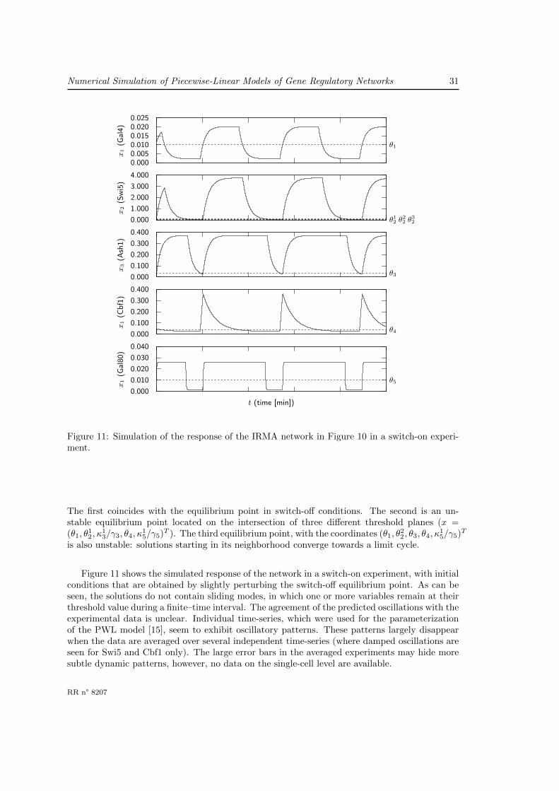
Numerical Simulation of Piecewise-Linear Models of Gene Regulatory Networks 31
0.0000.0050.0100.0150.0200.025
x1
(Gal
4)
θ1
0.0001.0002.0003.0004.000
x2
(Sw
i5)
θ12 θ22 θ
32
0.0000.1000.2000.3000.400
x3
(Ash
1)
θ3
0.0000.1000.2000.3000.400
x1
(Cbf
1)
θ4
0.0000.0100.0200.0300.040
x1
(Gal
80)
t (time [min])
θ5
Figure 11: Simulation of the response of the IRMA network in Figure 10 in a switch-on experi-ment.
The first coincides with the equilibrium point in switch-off conditions. The second is an un-stable equilibrium point located on the intersection of three different threshold planes (x =(θ1, θ
12, κ
13/γ3, θ4, κ
15/γ5)T ). The third equilibrium point, with the coordinates (θ1, θ
22, θ3, θ4, κ
15/γ5)T
is also unstable: solutions starting in its neighborhood converge towards a limit cycle.
Figure 11 shows the simulated response of the network in a switch-on experiment, with initialconditions that are obtained by slightly perturbing the switch-off equilibrium point. As can beseen, the solutions do not contain sliding modes, in which one or more variables remain at theirthreshold value during a finite–time interval. The agreement of the predicted oscillations with theexperimental data is unclear. Individual time-series, which were used for the parameterizationof the PWL model [15], seem to exhibit oscillatory patterns. These patterns largely disappearwhen the data are averaged over several independent time-series (where damped oscillations areseen for Swi5 and Cbf1 only). The large error bars in the averaged experiments may hide moresubtle dynamic patterns, however, no data on the single-cell level are available.
RR n° 8207
32 Acary, V., de Jong, H. & B. Brogliato
7 Discussion
We have presented a numerical method for the simulation of gene regulatory networks describedby PWL models. In order to account for discontinuities in the right-hand side of the differentialequations, PWL models have to be extended to differential inclusions which cannot be handled byclassical ODE solvers. We show that by reformulating one such extension, the AP-extension, asa mixed complementarity system (MCS), numerical methods developed for the time-integrationof nonsmooth dynamical systems are directly applicable. An extensive amount of work on themathematical and numerical analysis of complementarity systems has been done, which providesa solid theoretical basis for the proposed method. Moreover, powerful and widely-used numericaltools for complementarity systems are available, like the Siconos platform used here.
We have shown that under assumptions that are not restrictive in practice, the AP-extensionsare equivalent with other proposed extensions of PWL models, notably classical F-extensions(Proposition 11). The existence of solutions, which is guaranteed for F-extensions, therefore car-ries over to AP-extensions. Under the same assumptions, the AP-extensions are also equivalentwith hyperrectangular overapproximations of F-extensions that have been used in qualitativesimulations (Corollary 12). This has the advantage that the numerical analysis of PWL modelscan be preceded by the symbolic computation of equilibrium points and (in some cases) the an-alytic determination of their stability [27], as was done for the examples discussed in Section 6.More generally, the equivalency of the above-mentioned differential inclusions shows that thenumerical method developed here is applicable for different solution concepts of PWL modelsproposed in the literature.
The practical usefulness of the approach was illustrated by means of the numerical analysisof three actual biological networks in synthetic biology. We developed PWL models for thecircuits, either from scratch or by adapting existing ODE models, and parametrized the modelswith the help of literature data. For each of the models, we determined the equilibrium pointsand their stability, and we numerically computed solutions of the characteristic time-behavior ofthe networks. Although PWL models are coarse-grained approximations of the actual biologicalprocesses taking place in the cell, and the dynamics of PWL models may differ from those ofODE models [60], many of the observed dynamical properties of the synthetic networks could bereproduced by the simulations, such as the occurrence of stable oscillations in the repressilator(Section 6.1) and damped oscillations in the oscillator with positive feedback (Section 6.2).
The formulation of PWL models in the complementarity systems framework provides accessto powerful numerical tools for the analysis of dynamic properties of naturally-occurring networks[1, 67] or for the design of control schemes for synthetic networks [32]. Moreover, it also opensup the possibility to exploit results obtained for complementarity systems in the context of theanalysis of PWL models. For example, as a first step in this direction, we showed in Section 5.1that the strong monotonicity of the differential inclusion obtained after reformulating the PWLmodel as a MCS can be used to assure that an equilibrium point is (finite-time) stable.
A Alternative AP-extension of PWL models
As discussed in Section 3.1, the definition of AP-extensions could be relaxed by substitutingdifferent values σkj ∈ S+(xj , θ
kj ) for the different occurrences of s+(xj , θ
kj ), and by decoupling
the values for positive and negative step functions. This gives rise to an alternative AP-extensionof the PWL model (1).
Definition 18 (Alternative AP-extension of PWL models). The alternative AP-extension of a
Inria
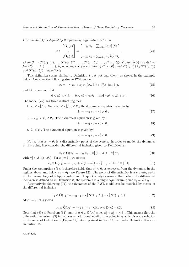
Numerical Simulation of Piecewise-Linear Models of Gene Regulatory Networks 33
PWL model (1) is defined by the following differential inclusion
x ∈
G1(x)...
Gn(x)
=
−γ1 x1 +∑l∈L1
κl1 bl1(S)
...
−γn xn +∑l∈Ln
κln bln(S)
. (74)
where S = (S+(x1, θ11), . . . , S+(x1, θ
p11 ), . . . , S+(xn, θ
1n), . . . , S+(xn, θ
pnn ))T , and bli(·) is obtained
from bli(·), i ∈ 1, . . . , n, by replacing every occurrence of s+(xj , θkj ) and s−(xj , θ
kj ) by S+(xj , θ
kj )
and S−(xj , θkj ), respectively.
This definition seems similar to Definition 8 but not equivalent, as shown in the examplebelow. Consider the following simple PWL model:
x1 = −γ1 x1 + κ11 s−(x1, θ1) + κ2
1 s+(x1, θ1), (75)
and let us assume that
0 < κ11 < γ1θ1, 0 < κ2
1 < γ1θ1, and γ1θ1 < κ11 + κ2
1. (76)
The model (75) has three distinct regimes:
1. x1 < κ11/γ1. Since x1 < κ1
1/γ1 < θ1, the dynamical equation is given by:
x1 = −γ1 x1 + κ11 > 0 . (77)
2. κ11/γ1 < x1 < θ1. The dynamical equation is given by:
x1 = −γ1 x1 + κ11 < 0 . (78)
3. θ1 < x1. The dynamical equation is given by:
x1 = −γ1 x1 + κ21 < 0 . (79)
Notice that x1 = θ1 is a discontinuity point of the system. In order to model the dynamicsat this point, first consider the differential inclusion given by Definition 8:
x1 ∈ G(x1) = −γ1 x1 + κ11 (1− σ1
1) + κ21 σ
11 , (80)
with σ11 ∈ S+(x1, θ1). For x1 = θ1, we obtain
x1 ∈ G(x1) = −γ1 x1 + κ11(1− σ1
1) + κ21 σ
11 , with σ1
1 ∈ [0, 1]. (81)
Under the assumption (76), it therefore holds that x1 < 0, as expected from the dynamics in theregions above and below x1 = θ1 (see Figure 12). The point of discontinuity is a crossing pointin the terminology of Filippov solutions. A quick analysis reveals that, when the differentialinclusion is defined as in Definition 8, the system has a single equilibrium point x1 = κ1
1/γ1.Alternatively, following (74), the dynamics of the PWL model can be modeled by means of
the differential inclusion
x1 ∈ G(x1) = −γ1 x1 + κ11 S−(x1, θ1) + κ2
1 S+(x1, θ1). (82)
At x1 = θ1 this yields:
x1 ∈ G(x1) = −γ1 x1 + σ, with σ ∈ [0, κ11 + κ2
1]. (83)
Note that (83) differs from (81), and that 0 ∈ G(x1) since κ11 + κ2
1 > γ1θ1. This means that thedifferential inclusion (83) introduces an additional equilibrium point in θ1 which is not a solutionin the sense of Definition 8 (Figure 12). As explained in Sec. 3.1, we prefer Definition 8 aboveDefinition 18.
RR n° 8207
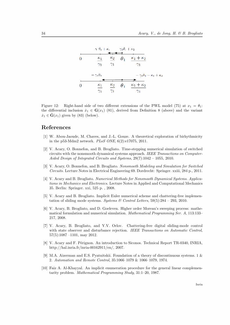
34 Acary, V., de Jong, H. & B. Brogliato
Figure 12: Right-hand side of two different extensions of the PWL model (75) at x1 = θ1:the differential inclusion x1 ∈ G(x1) (81), derived from Definition 8 (above) and the variant
x1 ∈ G(x1) given by (83) (below).
References
[1] W. Abou-Jaoude, M. Chaves, and J.-L. Gouze. A theoretical exploration of birhythmicityin the p53-Mdm2 network. PLoS ONE, 6(2):e17075, 2011.
[2] V. Acary, O. Bonnefon, and B. Brogliato. Time-stepping numerical simulation of switchedcircuits with the nonsmooth dynamical systems approach. IEEE Transactions on Computer-Aided Design of Integrated Circuits and Systems, 29(7):1042 – 1055, 2010.
[3] V. Acary, O. Bonnefon, and B. Brogliato. Nonsmooth Modeling and Simulation for SwitchedCircuits. Lecture Notes in Electrical Engineering 69. Dordrecht: Springer. xxiii, 284 p., 2011.
[4] V. Acary and B. Brogliato. Numerical Methods for Nonsmooth Dynamical Systems. Applica-tions in Mechanics and Electronics. Lecture Notes in Applied and Computational Mechanics35. Berlin: Springer. xxi, 525 p. , 2008.
[5] V. Acary and B. Brogliato. Implicit Euler numerical scheme and chattering-free implemen-tation of sliding mode systems. Systems & Control Letters, 59(5):284 – 293, 2010.
[6] V. Acary, B. Brogliato, and D. Goeleven. Higher order Moreau’s sweeping process: mathe-matical formulation and numerical simulation. Mathematical Programming Ser. A, 113:133–217, 2008.
[7] V. Acary, B. Brogliato, and Y.V. Orlov. Chattering-free digital sliding-mode controlwith state observer and disturbance rejection. IEEE Transactions on Automatic Control,57(5):1087 –1101, may 2012.
[8] V. Acary and F. Perignon. An introduction to Siconos. Technical Report TR-0340, INRIA,http://hal.inria.fr/inria-00162911/en/, 2007.
[9] M.A. Aizerman and E.S. Pyatnitskii. Foundation of a theory of discontinuous systems. 1 &2. Automation and Remote Control, 35:1066–1079 & 1066–1079, 1974.
[10] Faiz A. Al-Khayyal. An implicit enumeration procedure for the general linear complemen-tarity problem. Mathematical Programming Study, 31:1–20, 1987.
Inria
Numerical Simulation of Piecewise-Linear Models of Gene Regulatory Networks 35
[11] U. Alon. An Introduction to Systems Biology: Design Principles of Biological Circuits.Chapman & Hall/CRC, Boca Raton, FL, 2007.
[12] M.R. Atkinson, M.A. Savageau, J.T. Myers, and A.J. Ninfa. Development of genetic circuitryexhibiting toggle switch or oscillatory behavior in Escherichia coli. Cell, 113(5):597–608,2003.
[13] G. Batt, B. Besson, P.E. Ciron, H. de Jong, E. Dumas, J. Geiselmann, R. Monte, P.T.Monteiro, M. Page, F. Rechenmann, and D. Ropers. Genetic Network Analyzer: a toolfor the qualitative modeling and simulation of bacterial regulatory networks. In J. vanHelden, A. Toussaint, and D. Thieffry, editors, Bacterial Molecular Networks: Methods andProtocols, volume 804 of Methods in Molecular Biology, pages 439–462. Springer, New York,2012.
[14] G. Batt, H. de Jong, M. Page, and J. Geiselmann. Symbolic reachability analysis of geneticregulatory networks using discrete abstractions. Automatica, 44(4):982–989, 2008.
[15] G. Batt, M. Page, I. Cantone, G. Goessler, P.T. Monteiro, and H. de Jong. Efficient param-eter search for qualitative models of regulatory networks using symbolic model checking.Bioinformatics, 26(18):i603–i610, 2010.
[16] S.C. Billups. Algorithms for Complementarity Problems and Generalized Equations. PhDthesis, University of Wisconsin, Madison, 1995. available as Technical Report MP-TR-1995-14.
[17] S.C. Billups, S.P. Dirkse, and M.C. Ferris. A comparison of large scale mixed complemen-tarity problem solvers. Computational Optimization and Applications, 7:3–25, 1997.
[18] H. Bolouri. Computational Modeling of Gene Regulatory Networks – A Primer. ImperialCollege Press, London, 2008.
[19] B. Brogliato. Absolute stability and the Lagrange-Dirichlet theorem with monotone multi-valued mappings. Systems & Control Letters, 51(5):343 – 353, 2004.
[20] B. Brogliato, A. Daniilidis, C. Lemarechal, and V. Acary. On the equivalence betweencomplementarity systems, projected systems and differential inclusions. Systems & ControlLetters, 55:45–51, 2006.
[21] M. K. Camlibel, W.P.M.H. Heemels, and J.M. Schumacher. Consistency of a time-steppingmethod for a class of piecewise-linear networks. IEEE Transacations on Circuits and systemsI, 49:349–357, 2002.
[22] I. Cantone, L. Marucci, F. Iorio, M.A. Ricci, V. Belcastro, M. Bansal, S. Santini,M. di Bernardo, D. di Bernardo, and P.M. Cosma. A yeast synthetic network for in vivoassessment of reverse-engineering. Cell, 137(1):172–181, 2009.
[23] R. Casey, H. de Jong, and J.-L. Gouze. Piecewise-linear models of genetic regulatory net-works: Equilibria and their stability. Journal of Mathematical Biology, 52(1):27–56, 2006.
[24] C. Chaouiya, A. Naldi, and D. Thieffry. Logical modelling of gene regulatory networkswith GINsim. In J. van Helden, A. Toussaint, and D. Thieffry, editors, Bacterial MolecularNetworks: Methods and Protocols, volume 804 of Methods in Molecular Biology, pages 463–479. Springer, New York, 2012.
RR n° 8207
36 Acary, V., de Jong, H. & B. Brogliato
[25] R. W. Cottle, J. Pang, and R. E. Stone. The Linear Complementarity Problem. AcademicPr ess, Inc., Boston, MA, 1992.
[26] H. de Jong, J.-L. Gouze, C. Hernandez, M. Page, T. Sari, and J. Geiselmann. Qualita-tive simulation of genetic regulatory networks using piecewise-linear models. Bulletin ofMathematical Biology, 66(2):301–340, 2004.
[27] H. de Jong and M. Page. Search for steady states of piecewise-linear differential equationmodels of genetic regulatory networks. ACM/IEEE Transactions on Computational Biologyand Bioinformatics, 5(2):208–222, 2008.
[28] H. de Jong and D. Ropers. Strategies for dealing with incomplete information in the mod-eling of molecular interaction networks. Briefings in Bioinformatics, 7(4):354–363, 2006.
[29] S. P. Dirkse and M. C. Ferris. The PATH solver: A non-monotone stabilization scheme formixed complementarity problems. Optimization Methods and Software, 5:123–156, 1995.
[30] A.L. Dontchev and F. Lempio. Difference methods for differential inclusions: a survey.SIAM Reviews, 34(2):263–294, 1992.
[31] R. Edwards. Analysis of continuous-time switching networks. Physica D, 146(1-4):165–199,2000.
[32] R. Edwards, S. Kim, and P. van den Driessche. Control design for sustained oscillation ina two gene regulatory network. Journal of Mathematical Biology, 62(4):453–479, 2011.
[33] M.B. Elowitz and S. Leibler. A synthetic oscillatory network of transcriptional regulators.Nature, 403(6767):335–338, 2000.
[34] F. Facchinei and J. S. Pang. Finite-dimensional Variational Inequalities and Complemen-tarity Problems, volume I & II of Springer Series in Operations Research. Springer VerlagNY. Inc., 2003.
[35] E. Farcot and J.-L. Gouze. Periodic solutions of piecewise affine gene network modelswith non uniform decay rates: The case of a negative feedback loop. Acta Biotheoretica,57(4):429–455, 2009.
[36] M. C. Ferris and T. S. Munson. Interfaces to PATH 3.0: Design, implementation and usage.Comput. Optim. Appl., 12(1-3):207–227, 1999.
[37] A. F. Filippov. Differential Equations with Discontinuous Right Hand Sides. Kluwer, Dor-drecht, the Netherlands, 1988.
[38] C. Georgescu, B. Brogliato, and V. Acary. Switching, relay and complementarity systems:A tutorial on their well-posedness and relationships. Physica D: Nonlinear Phenomena,241(22):1985 – 2002, 2012.
[39] L. Glass and S.A. Kauffman. The logical analysis of continuous non-linear biochemicalcontrol networks. Journal of Theoretical Biology, 39(1):103–129, 1973.
[40] L. Glass and J.S. Pasternack. Stable oscillations in mathematical models of biological controlsystems. Journal of Mathematical Biology, 6:207–223, 1978.
[41] L. Glass and H.T. Siegelmann. Logical and symbolic analysis of robust biological dynamics.Current Opinion in Genetics & Development, 20(6):644–649, 2010.
Inria
Numerical Simulation of Piecewise-Linear Models of Gene Regulatory Networks 37
[42] J.-L. Gouze and T. Sari. A class of piecewise linear differential equations arising in biologicalmodels. Dynamical Systems, 17(4):299–316, 2002.
[43] L. Han, A. Tiwari, K. Camlibel, and J.S. Pang. Convergence of time–stepping schemes forpassive and extended linear complementarity systems. SIAM Journal of Numerical Analysis,47(5):3768–3796, 2009.
[44] W.P.M.H. Heemels, J.M. Schumacher, and S. Weiland. Linear complementarity systems.SIAM Journal Applied Mathematics, 60:1234–1269, 2000.
[45] R. Hengge-Aronis. The general stress response in Escherichia coli. In G. Storz andR. Hengge-Aronis, editors, Bacterial Stress Responses, pages 161–177. ASM Press, Wash-ington, DC, 2000.
[46] J.B. Hiriart-Urruty and C. Lemarechal. Fundamentals of Convex Analysis. Springer Verlag,2001.
[47] L. Ironi and L. Panzeri. A computational framework for qualitative simulation of nonlineardynamical models of gene-regulatory networks. BMC Bioinformatics, 10(Suppl 12):S14,2009.
[48] N.H. Josephy. Newton’s method for generalized equations. Technical report, MathematicsResearch Center, University of Wisconsin, Madison., 1979.
[49] J. Judice, A. Faustino, and I. Ribeiro. On the solution of NP-hard linear complementarityproblems. TOP, 10:125–145, 2002. 10.1007/BF02578944.
[50] G. Karlebach and R. Shamir. Modelling and analysis of gene regulatory networks. NatureReviews Molecular Cell Biology, 9(10):770–780, 2008.
[51] A.S. Khalil and J.J. Collins. Synthetic biology: applications come of age. Nature ReviewsGenetics, 11(5):367–379, 2010.
[52] Z. Kohavi and N.J. Jha. Switching and Finite Automata Theory. Cambridge UniversityPress, third edition, 2010.
[53] A. Machina and A. Ponosov. Filippov solutions in the analysis of piecewise linear modelsdescribing gene regulatory networks. Nonlinear Analysis. Theory, Methods and Applications,74(3):882–900, 2011.
[54] L. Marucci, D.A.W. Barton, I. Cantone, M.A. Ricci, M.P. Cosma, S. Santini, D. di Bernardo,and M. di Bernardo. How to turn a genetic circuit into a synthetic tunable oscillator, or abistable switch. PLoS ONE, 4(12):E8083, 2011.
[55] T. Mestl, E. Plahte, and S.W. Omholt. A mathematical framework for describing andanalysing gene regulatory networks. Journal of Theoretical Biology, 176(2):291–300, 1995.
[56] Y.V. Orlov. Discontinuous Systems. Communications and Control Engineering. SpringerVerlag, 2009.
[57] J.-S. Pang and D. Stewart. Differential variational inequalities. Mathematical ProgrammingA, 113(2), 2008.
[58] E. Plahte and S. Kjoglum. Analysis and generic properties of gene regulatory networks withgraded response functions. Physica D, 201(1):150–176, 2005.
RR n° 8207
38 Acary, V., de Jong, H. & B. Brogliato
[59] E. Plahte, T. Mestl, and S.W. Omholt. A methodological basis for description and analysis ofsystems with complex switch-like interactions. Journal of Mathematical Biology, 36(4):321–348, 1998.
[60] A. Polynikis, S.J. Hogan, and M. di Bernardo. Comparing different ODE modelling ap-proaches for gene regulatory networks. Journal of Theoretical Biology, 261(4):511–530, 2009.
[61] O. Purcell, N.J. Savery, C.S. Grierson, and M. di Bernardo. A comparative analysis ofsynthetic genetic oscillators. Journal of the Royal Society Interface, 7(52):1503–1524, 2010.
[62] R.T. Rockafellar and R.J.B. Wets. Variational Analysis, volume 317. Springer Verlag, NewYork, 1998.
[63] T. Rutherford. Miles: A mixed inequality and nonlinear equation solver, 1993.
[64] H.D. Sherali, R.S. Krishnamurthy, and F.A. Al-Khayyal. Enumeration approach for lin-ear complementarity problems based on a reformulation-linearization technique. JournalOptimization Theory and Applications, 99(2):481–507, 1998.
[65] D. Stewart. A high accuracy method for solving ODEs with discontinuous rigth–hand–side.Numerische Mathematik, 58:299–328, 1990.
[66] R. Thomas and R. d’Ari. Biological Feedback. CRC Press, Boca Raton, FL, 1990.
[67] L. Tournier and M. Chaves. Uncovering operational interactions in genetic networks usingasynchronous Boolean dynamics. Journal of Theoretical Biology, 260(2):196–209, 2009.
[68] J.J. Tyson and H.G. Othmer. The dynamics of feedback control circuits in biochemicalpathways. Progress in Theoretical Biology, 5:1–62, 1978.
[69] V.I. Utkin. Variable structure systems with sliding modes: A survey. IEEE Transactionson Automatic Control, 22:212–222, 1977.
[70] V.I. Utkin. Sliding Modes in Control Optimization. SpringerVerlag. Berlin., Berlin, 1992.
Inria
Numerical Simulation of Piecewise-Linear Models of Gene Regulatory Networks 39
Contents
1 Introduction 3
2 PWL models of gene regulatory networks 42.1 Definition of PWL models . . . . . . . . . . . . . . . . . . . . . . . . . . . . . . . 42.2 Regulation functions in PWL models . . . . . . . . . . . . . . . . . . . . . . . . . 6
3 Solutions of PWL models 83.1 Filippov extensions of PWL models . . . . . . . . . . . . . . . . . . . . . . . . . . 83.2 Relations between different Filippov extensions of PWL models . . . . . . . . . . 10
4 Numerical methods for AP-extensions of PWL systems 134.1 Reformulation of PWL models as Mixed Complementarity Systems (MCS) . . . 134.2 The general time-discretization framework. . . . . . . . . . . . . . . . . . . . . . 154.3 An enumerative procedure based on the Newton–Josephy approach . . . . . . . . 174.4 Software aspects . . . . . . . . . . . . . . . . . . . . . . . . . . . . . . . . . . . . 18
5 Illustration of the properties of the numerical methods on a two-gene regula-tory network 195.1 MCS formulation and stability analysis . . . . . . . . . . . . . . . . . . . . . . . . 195.2 Properties of the numerical simulations . . . . . . . . . . . . . . . . . . . . . . . 21
6 Applications in synthetic biology 246.1 Repressilator . . . . . . . . . . . . . . . . . . . . . . . . . . . . . . . . . . . . . . 246.2 Synthetic oscillator with positive feedback . . . . . . . . . . . . . . . . . . . . . . 256.3 IRMA: a synthetic benchmark network . . . . . . . . . . . . . . . . . . . . . . . . 28
7 Discussion 32
A Alternative AP-extension of PWL models 32
RR n° 8207

RESEARCH CENTREGRENOBLE – RHÔNE-ALPES
Inovallée655 avenue de l’Europe Montbonnot38334 Saint Ismier Cedex
PublisherInriaDomaine de Voluceau - RocquencourtBP 105 - 78153 Le Chesnay Cedexinria.fr
ISSN 0249-6399