Embed Size (px)
Citation preview
UC BerkeleyTechnical Completion Reports
TitleNumerical Simulation of Land Subsidence in the Los Banos-Kettleman City Area, California
Permalinkhttps://escholarship.org/uc/item/6140n0w6
AuthorsLarson, Keith JBasagaoglu, HakanMarino, Miguel A
Publication Date1999-10-01
eScholarship.org Powered by the California Digital LibraryUniversity of California
G402 -{XU2-7 ~l/ul
Numerical Simulation of Land Subsidencein the Los Banos-Kettleman City Area, California
ByKeith J. Larson I, Hakan Basagaoglu 1 and Miguel A. Marifio''
IDepartment of Civil & Environmental Engineering2Department of Land, Air, and Water Resources andDepartment of Civil & Environmental Engineering
University of California, DavisDavis, CA 95616
TECHNICAL COMPLETION REPORT
Project Number UCAL-WRC-W-892
October 1999
University of California Water Resources Center
VVA~f"E':F~F~E'.~;()lJ t:.sCt:f\!TE:;; /\F)CHiVE~;
JA~1 ". -- Z(JOO
The research leading to this report was supported by the University of California WaterResources Center, as part of Water Resources Center Project UCAL-WRC-W-892.
ABSTRACT
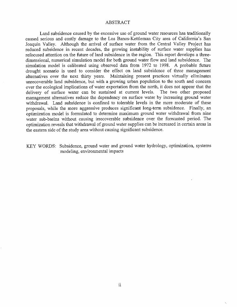
Land subsidence caused by the excessive use of ground water resources has traditionallycaused serious and costly damage to the Los Banos-Kettleman City area of California's SanJoaquin Valley. Although the arrival of surface water from the Central Valley Project hasreduced subsidence in recent decades, the growing instability of surface water supplies hasrefocused attention on the future of land subsidence in the region. This report develops a three-dimensional, numerical simulation model for both ground water flow and land subsidence. Thesimulation model is calibrated using observed data from 1972 to 1998. A probable futuredrought scenario is used to consider the effect on land subsidence of three managementalternatives over the next thirty years. Maintaining present practices virtually eliminatesunrecoverable land subsidence, but with a growing urban population to the south and concernover the ecological implications of water exportation from the north, it does not appear that thedelivery of surface water can be sustained at current levels. The two other proposedmanagement alternatives reduce the dependency on surface water by increasing ground waterwithdrawal. Land subsidence is confined to tolerable levels in the more moderate of theseproposals, while the more aggressive produces significant long-term subsidence. Finally, anoptimization model is formulated to determine maximum ground water withdrawal from ninewater sub-basins without causing irrecoverable subsidence over the forecasted period. Theoptimization reveals that withdrawal of ground water supplies can be increased in certain areas inthe eastern side of the study area without causing significant subsidence.
KEY WORDS: Subsidence, ground water and ground water hydrology, optimization, systemsmodeling, environmental impacts
11
TABLE OF CONTENTS
Abstract ... . .. .. . . .. . . . .. . .. . . .. .. . ... .. .. .. . .. . .. . . .. . .. . . .. . .. . .. .. .. .. .. .. .. . .. .. . .. . . .. . . .. . . . .. .. 11
List of Tables IV
List of Figures V
1. Introduction. . .. . . .. . .. . . .. .. .. .. .. .. .. . .. . .. . . .. . . .. . .. . .. .. . .. .. .. .. .. .. .. .. . . .. . . .. . . .. . . .. 12. Background. . .. . . .. . . . . .. . .. .. . ... ... . .. .. . . .. .. .. .. .. . . .. .. . 2
2.1 Subsidence in the San Joaquin Valley............. 22.2 The Los Banos-Kettleman City Region................................................ 4
2.2.1 Hydrogeology...... .. . ... ... ... .. . . .. . .. .. .. ..... ... . .. .. .... .. . .. . . .. . . . .. . . .. . .. 62.2.2 Water Budget..................................................................... 82.2.3 Surface Water Supplies................................ 10
2.3 Numerical Models.................................................................... 102.3.1 The Ground Water Flow Model 102.3.2 The Land Subsidence Model 11
3. Application of Model... .. . . .. .. ... ... .. . . ... .. . . .. . .. . . . ... . .. . .. . . . . 173.1 Modification of the Belitz et al. (1992) Ground Water Flow Model............... 17
3.1.1 Geometry. . .. .. .. . ... .. . .. .. . .. . . .. . .. . . .. . .. .. . .. .. .. .. .. .. .. . .. . .. . . .. . . .. . ... .... 173.1.2 Pumping 213.1.3 Initial and Preconsolidation Heads... . . .. ... .. ... . ... . .. .. .. .. 253.1.4 Other Modifications 28
3.2 Calibration 293.2.1 Piezometric Head 293.2.2 Land Subsidence 38
3.3 Sensitivity Analysis 453.3.1 Hydraulic Conductivity 453.3.2 Elastic and Inelastic Storage Coefficients 453.3.3 Preconsolidation Heads 47
4. Predicting Future Subsidence Potential , 504.1 Development of Future Drought Scenarios.. . .. .. . .. .. .. . .. .. . .. 504.2 Potential Management Alternatives 544.3 Optimization Model 594.4 Results '" 64
5. Conclusions and Recommendations 71References 76Appendix 80
1ll
LIST OF TABLES
Table l.Table 2.Table 3.Table 4.Table 5.Table 6.
Revised water budget for 1980 (Modified from Gronberg and Belitz, 1992)... 9Yearly CVP deliveries for Westlands and Panoche Water Districts 23Well numbers for extensometers and monitoring wells 30Future water delivery scenario , . , , 57Alternative B proposed water budget (From Belitz and Phillips, 1995) ,.. 60Maximum Drawdowns and Areas for Pumping Subareas , .. , .. 63
IV
LIST OF FIGURES
Figure 1. Map of California showing the location of the San Joaquin Valley 3Figure 2. Location of Study Area and Water Budget Subareas 5Figure 3. Hydrogeologic cross-section of the study area (Modified from Belitz et al.,
1992) 7Figure 4. Role of pore pressure in the time delay of consolidation 15Figure 5. Model grid and location of observation wells 18Figure 6. Modifications made to the Belitz et al. (1992) model layers 19Figure 7. Relationship between CVP water delivery and ground water pumping rates 24Figure 8. Schematic drawing of initial and preconsolidation heads for the time of
maximum drawdown " 26Figure 9. Observed and simulated piezometric head for observation location 1 31Figure 10. Observed and simulated piezometric head for observation location 2 31Figure 11. Observed and simulated piezometric head for observation location 3 32Figure 12. Observed and simulated piezometric head for observation location 4 32Figure 13. Observed and simulated piezometric head for observation location 5 33Figure 14. Observed and simulated piezometric head for observation location 6 33Figure 15. Observed and simulated piezometric head for observation location A 34Figure 16. Observed and simulated piezometric head for observation location B 34Figure 17. Observed and simulated piezometric head for observation location C 35Figure 18. Observed and simulated piezometric head for observation location D 35Figure 19. Observed and simulated piezometric head for observation location E 36Figure 20. Observed and simulated piezometric head for observation location F 36Figure 21. Observed and simulated piezometric head for observation location G 37Figure 22. Observed and simulated land subsidence for extensometer 1 40Figure 23. Observed and simulated land subsidence for extensometer 2 40Figure 24. Observed and simulated land subsidence for extenso meter 3 41Figure 25. Observed and simulated land subsidence for extenso meter 4 41Figure 26. Observed and simulated land subsidence for extensometer 5 ,. 42Figure 27. Observed and simulated land subsidence for extensometer 6 42Figure 28. (a) Observed land subsidence for the Los Banos-Kettleman City area, 1926-
72 (Ireland et al., 1984); (b) Simulated land subsidence for the Los Banos-Kettleman City area, 1972-98 43
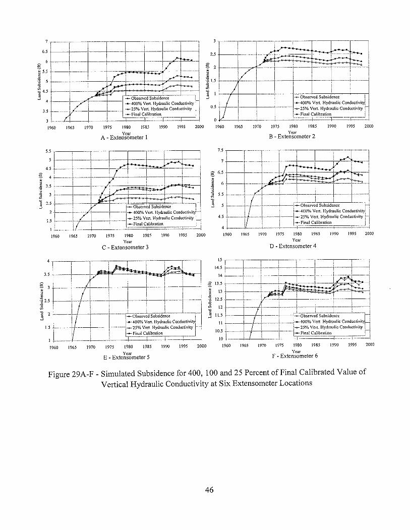
Figure 29. (a)-(t) Simulated land subsidence for 400, 100, and 25 percent of finalcalibrated value of vertical hydraulic conductivity at six extensometerlocations 46
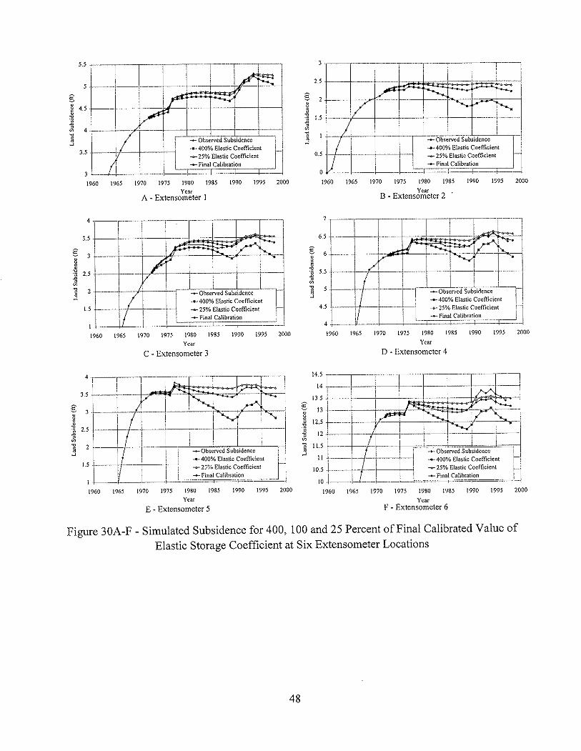
Figure 30. (a)-(t) Simulated land subsidence for 400, 100, and 25 percent of finalcalibrated value of elastic storage coefficient at six extensometer locations .... 48
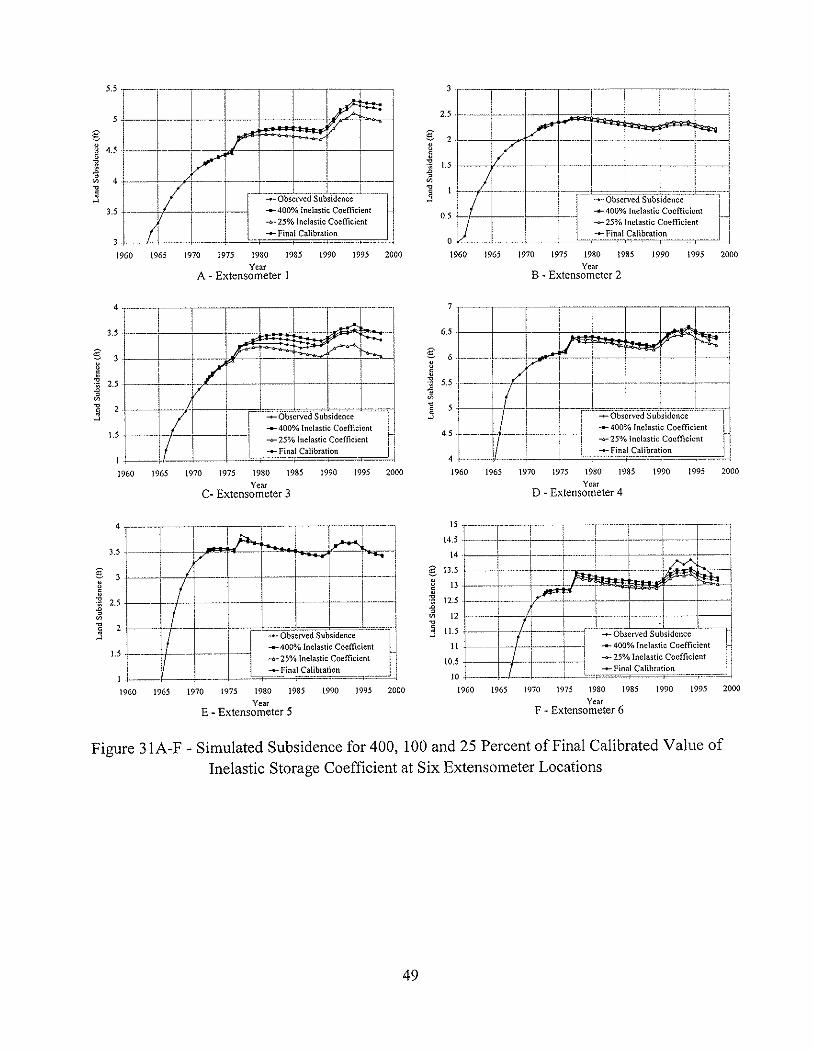
Figure 31. (a)-Ct) Simulated land subsidence for 400,100, and 25 percent of finalcalibrated value of inelastic storage coefficient at six extensometer locations ..49
Figure 32. (a)-(f) Simulated land subsidence for 125, 100, and 75 percent of finalcalibrated value of residual pore pressure at six extensometer locations 51
Figure 33. Best fit relationship between the Sacramento four-rivers index and theCentral Valley Project surface water delivery rate for "below average," dry,"and "critical" water years 53
v
Figure 34. Cumulative distribution function for the average drought of drought yearsduring the thirty year water availability scenario 55
Figure 35. Cumulative distribution function for the cumulative deficit of drought yearsduring the thirty year water availability scenario 56
Figure 36. The relationship between the Sacramento four-rivers index and the CentralValley Project surface water delivery rate for three management alternatives ..58
Figure 37. Model predictions of total subsidence for 1999-2028 at extensometer 1. 65Figure 38. Model predictions of total subsidence for 1999-2028 at extensometer 2 '" 65Figure 39. Model predictions of total subsidence for 1999-2028 at extensometer 3 66Figure 40. Model predictions of total subsidence for 1999-2028 at extensometer 4 66Figure 41, Model predictions of total subsidence for 1999-2028 at extensometer 5 67Figure 42. Model predictions of total subsidence for 1999-2028 at extensometer 6 67Figure 43. Contour map of simulated subsidence, 1999-2028 (Alternative A) 68Figure 44. Contour map of simulated subsidence, 1999-2028 (Alternative B) '" 69Figure 45, Contour map of simulated subsidence, 1999-2028 (Alternative C) 70Figure 46. Maximum Ground Water Withdrawal from Optimization Model 72
VI
1. INTRODUCTION
The San Joaquin Valley is an important agricultural region in California, contributing
billions of dollars to the state's economy and providing jobs and food for the state's growing
population. As such, providing affordable water for agriculture has traditionally been a high
priority for water managers in the region. In recent years, however, a limited water supply has
created economic and environmental concerns that threaten the viability of agriculture in
portions of the Valley.
One of the more subtle of these concerns is land subsidence. Land subsidence is defined
as a lowering of the land surface elevation. Although this geologicallhydrological hazard
progresses slowly, it can result in significant economic losses over time (Hua et al., 1993). In the
San Joaquin Valley, land subsidence has caused serious and costly damage to highways, water-
transport structures and deep water wells (Ireland et aL, 1984). Although there are several causes
of land subsidence, the majority of subsidence in the Valley can be attributed to overpumping of
the aquifer system underlying the region.
Prior to 1967, the main source of irrigation water was ground water. As unregulated
pumping accompanied rapid agricultural development, dramatic drawdown occurred in the
aquifers underlying the region. One result of this drawdown was severe land subsidence
throughout much of the Valley. In 1967, the completion of the California Aqueduct provided a
new source of water for irrigation. As canals and delivery systems were completed, the demand
for ground water was reduced and land subsidence rates correspondingly decreased. However,
the inevitability of drought and the continued growth of urban areas to the south made the
aqueduct a less than reliable alternative. This was made evident in 1977 and the early 1990s as
drought forced a renewed dependence on ground water and the return of subsidence.
The goal of this research is to evaluate the effects of existing and proposed water
management plans on land subsidence in the Los Banos-Kettleman City region of the San
Joaquin Valley. This will be accomplished through: (1) employment of existing numerical
models to simulate ground water flow and land subsidence over the Los Banos-Kettleman City
region; (2) calibration of the overall model using observed ground water and compaction data for
the years 1972 to 1999; (3) identification of the most influential aquifer parameters and their
roles in model calibration; (4) construction of future water availability scenarios; and (5)
implementation of the calibrated model to estimate future land subsidence to test the existing and
proposed management alternatives.
2. BACKGROUND
2.1 Subsidence in the San Joaquin Valley
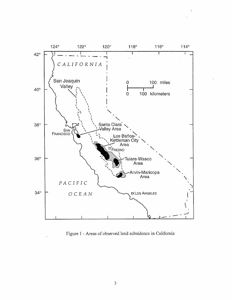
California's San Joaquin Valley (Figure 1) is one of the most productive and intensely
farmed agricultural areas in the world (American Farmland Trust, 1995). The Valley has been
experiencing land subsidence and its negative implications as early as the 1920s (Ireland et al.,
1984). Intense abstractions of ground water in excess of natural recharge caused ground water
storage depletion and resulting land subsidence across the Valley. In 1969, subsidence reached
nearly 29 feet in one location with a total volume of 15.5 MAF (Poland, 1981).
Subsidence can have several negative economic, social, and technical implications.
Problems associated with land subsidence include: (1) changes in ground water and surface
water flow patterns (e.g., Lofgren, 1979); (2) ground water quality deterioration and salt-water
encroachment (e.g., Belitz and Philips, 1995); (3) decline in aquifer storage capacity; (4)
flooding (e.g., Hua et al., 1993); (5) failure of well casings and changes in channel gradient (e.g.,
Holzer, 1989); and (6) damage to highways, buildings, and other structures (e.g., Ireland et al.,
2
San JoaquinValley 1"'\
-, I, \", \1 '\\ \I \I \\ \, I
r~ \\ I\ \ "'"...• \ .1\ -. Santa Clara <,\ ' Valley Area
Los Bano~." Kettleman City "'"", Area[]FRESNO
"/\
\ Tulare-WascoI AreaI
.... \
\ ~Arvin-Maricopa...~ Area
CALIFORNIA
PACIFIC
OCEAN
--,
o 100 miles1--..----.11I
o 100 kilometers
Figure 1 - Areas of observed land subsidence in California
3
1984). By the mid-1960s, several regions in the San Joaquin Valley were facing many of these
problems (e.g., Ireland, 1986).
The arrival of surface water supplies in the late 1960s greatly reduced the amount of
ground water withdrawn from the region. With the reduction in pump age, the rate of land
subsidence slowed down. During droughts in 1976-77 and 1990-1992, however, ground water
supplies were pumped heavily to meet demand as surface water deliveries were reduced. In the
Los Banos-Kettleman City area, pumpage increased to 470,000 acre-feet in 1977 compared to a
yearly average of less than 100,000 acre-feet from 1974 to 1976 (Ireland et al., 1984). The
result was a return to subsidence rates comparable to those before the arrival of surface water.
In addition to drought, several other factors threaten future surface water supplies to the
San Joaquin Valley. The growth of urban populations to the south places an increasing strain on
existing imported water supplies. There is also growing concern over the ecological impact of
exportation of water from the north. The surface water for the Valley remains precariously
balanced between competing urban, environmental, and agricultural interests. Although recent
measurements reveal that annual average land subsidence rates have declined over the last three
decades, the volatile future of surface water in the region maintains land subsidence as a serious
concern to local and state water agencies (California Department of Water Resources, 1998).
2.2 The Los Banos-Kettleman City Region
Three areas of the San Joaquin Valley exhibit especially severe subsidence: the Los
Banos-Kettleman City area, the Tulare-Wasco area, and the Arvin-Maricopa area. The area
chosen for this research comprises the northern portion of the Los Banos-Kettleman City area.
This 550-square-mile region of western Fresno County (Figure 2) has been chosen because of the
large amount of ground water and land subsidence data available. Additionally, several previous
4
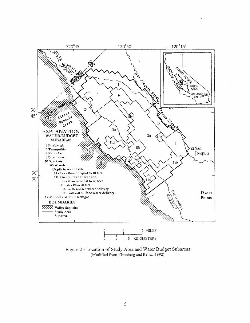
1 Firebaugh6 Tranquility8 Panoche9 Broadview10 San Luis
WestlandsDepth to water tablel1a Less than or equal to 10 feetllb Greater than 10 feet and
less than or equal eo 20 feetGreater than 20 feetHe with surface water delivery11dwithout surface water delivery
12Mendota Wildlife Refugre
BOUNDARIES~ Valley deposits-- Study Area-- Subarea
o 5 to MILESI I I I Io 5 10 KILOMETERS
Figure 2 - Location of Study Area and Water Budget Subareas(Modified from Gronberg and Belitz, 1992)
5
o SanJoaquin
FiveDPoints
studies have been conducted in the region, providing important insight into several aspects of
this research.
2.2.1 Hydrogeology
The hydrogeology of the Los Banos Kettleman City area was previously documented by
Miller et al. (1971) and Belitz and Heimes (1990). From their reports, the subsurface flow
system is divided into upper and lower water-bearing zones, which are separated by the Corcoran
Clay Member of the Tulare Formation (Figure 3). The thickness of the Corcoran Clay Member
ranges from 20 to 120 ft (Page, 1986) and consists of low-conductivity lacustrine deposits
(Johnson et al., 1968).
The unconfined to semi -confined zone above the Corcoran Clay member consists of
Coast Ranges alluvium, Sierran sand, and flood basin deposits. The Coast Ranges alluvium
reaches a thickness of more than 800 ft near the western edge of the valley. It is composed of
sand and gravel along the stream channels and at the fan heads, and of clay and silt in the distal
fan areas (Laudon and Belitz, 1991). The Coast Ranges alluvium is interfingered laterally with
the Sierran sand, which consists of well-sorted medium to coarse-grained fluvial sand reaching a
thickness of 400-500 ft in the valley trough (Miller et al., 1971). Flood-basin deposits, with a
thickness of 5~35 ft, overlie the Sierran sand at the center of the valley (Laudon and Belitz,
1991). The quality of ground water of the upper water-bearing zone is generally poor with high
concentrations of calcium, magnesium, and sulfate, except near Fresno Slough (Bull and Miller,
1975).
The lower water-bearing zone is locally less permeable than the upper-water bearing
zone. It is also much thicker, ranging from 570 to 2460 ft (Williamson et al., 1989). In general,
it is composed of poorly consolidated flood-basin, deltaic, alluvial-fan, and lacustrine deposits of
6
600
400
San Joaquin River: : : : : : : : : : : :~:~:~:~:>~:::::::::~:::::<:::<,, ... , , ,)ood-Basin Deposits, , , . . , , , , , , ": -; , ; ,> :- ; -: ' :- :- :- ;": .:- :- :. .: >:' , , , , . , ';':':':'~:'~:' -:-:":-:.,.....:-.-,-..-
SeaLevel
... " ' , .. ' '."".~~~~
200
•••• L , L ••••••• L •••................. , L·.·.·.·.·.·.·.· L' .'. L. '.' .. "!!- " '" '" "" , lit. , lilt IIlo ".. , , . , .. CQasrRarig~.AlluVi·um:, , . ,.:,:.:-:.:,: .." ~H •••• -
••••••••••••••••••••• ' •••• '.·.·.'.· •••• L •••••••• • ••••• "II""''\'''''IM~'IM •••''''''''' •••.. . . . . . . . . . . . . . . . . .
-200
-400
-600
Low PermeabilityInterbeds ...:::::::---~-
Vertical Scale Greatly Exaggerated
Figure 3 - Hydrogeologic Cross-section of the Study Area(Modified from Belitz et aL,1992)
7
Tulare formation (Bull and Miller, 1975) characterized by discontinuous clay lenses embodied
with sand and gravel deposits. Before surface water supplies were made available to the Los
Banos-Kettleman City area through aqueducts and irrigation channels, 75-80% of irrigation
water was pumped from the lower water-bearing zone due to its greater thickness and better
water quality (Bull and Miller, 1975; Ireland et al., 1984).
2.2.2 Water Budget
Gronberg and Belitz (1992) performed an analysis of ground water pumpage, recharge,
and irrigation efficiency for the Los Banos-Kettleman City region. This analysis resulted in two
water budgets for the years 1980 and 1984. The Los Banos-Kettleman City area is divided into
nine water-budget subareas based on water district boundaries and depth to water table (Figure
2). An area-weighted average irrigation efficiency is calculated for each subarea as a function of
depth to water table. The irrigation efficiency is subsequently used to compute the irrigation
requirement in each water budget subarea. If the computed irrigation requirement exceeds
surface water delivery, the unmet water requirement is supplied from the ground water reservoir;
otherwise no pumpage takes place. The required ground water pumpage volume is spread
uniformly over each subarea.
Gronberg and Belitz (1992) did not consider drought in their water budget analysis.
However, drought will have a substantial influence on the rate and magnitude of land subsidence.
During normal water years, this report will adopt the same pumping rates and spatial distribution
between subareas as that computed by Gronberg and Belitz (1992) for the year 1980 (Table 1).
For drought periods, however, ground water pumping rates will be a function of available surface
water supplies. This will be discussed in greater detail in subsequent sections.
8
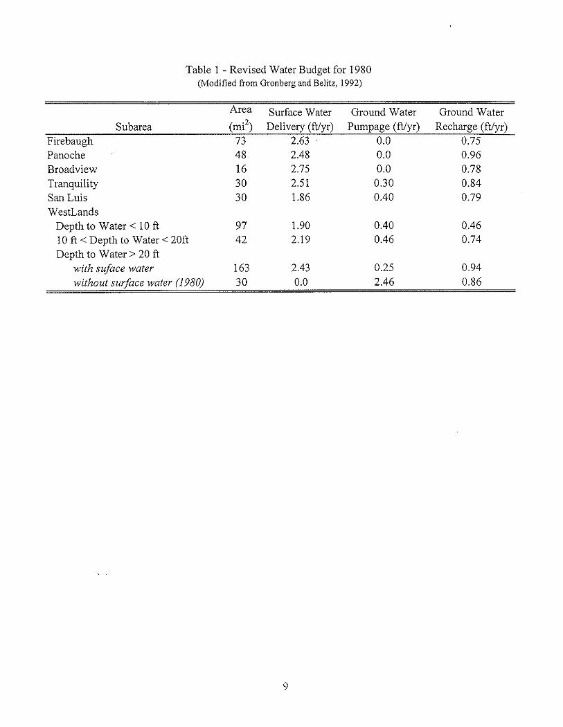
Table 1 - Revised Water Budget for 1980(Modified from Gronberg and Belitz, 1992)
Area Surface Water Ground Water Ground WaterSubarea (mi2) Delivery (ftJyr) Pumpage (ft/yr) Recharge (ftlyr)
Firebaugh 73 2.63 0.0 0.75Panoche 48 2.48 0.0 0.96Broadview 16 2.75 0.0 0.78Tranquility 30 2.51 0.30 0.84San Luis 30 1.86 0040 0.79WestLands
Depth to Water < lOft 97 1.90 0040 0.46lOft <Depth to Water < 20ft 42 2.19 0046 0.74Depth to Water> 20 ft
with suface water 163 2.43 0.25 0.94without surface water (1980) 30 0.0 2.46 0.86
9
2.2.3 Surface Water Supplies
The State Water Resources Control Board (SWRCB) issued the first water rights to the
U.S. Bureau of Reclamation (USBR) for operation of the Central Valley Project (CVP) in 1958
and to the California Department of Water Resources (DWR) for operation of the State Water
Project (SWP) in 1967. Principal facilities of the SWP include Oroville Dam, Delta facilities, the
California Aqueduct, and North and South Aqueducts. The principal facilities of CVP include
Shasta, Trinity, Folsom, Friant, Clair Engle, Whiskeytown, and New Melones dams, Delta
facilities, and the Delta Mendota Canal. Joint SWP/CVP facilities include San Luis Reservoir
and Canal and various Delta facilities (California Water Plan Update, 1998). Although it arrives
through an SWP facility (the California Aqueduct), all of the surface water used in the study
region is contracted through the CVP and delivery rates are determined by the USBR.
2.3 Numerical Models
2.3.1 The Ground Water Flow Model
Ground water levels for the Los Banos-Kettleman City area were previously modeled by Belitz
et al. (1992) using MODFLOW, a modular finite-difference flow model developed by McDonald
and Harbaugh (1988). MODFLOW is a three-dimensional ground water simulation model that
has been successfully used in real world problems involving aquifer simulation (e.g., Sophoc1eus
and Perkins, 1993; Reynolds and Spruill, 1995; Bumb et al., 1997; Hubbel et al., 1997). It can
simulate anisotropic and heterogeneous aquifer systems with various boundary conditions.
MODFLOW's structure is described as modular because it consists of one main program
surrounded by a group of "modules" or packages. Each package considers different aspects of
ground water flow. Packages are available to evaluate evaporation, recharge, drains, and land
10
subsidence to name a few. A modular structure is advantageous because it allows for the
addition of new features without much alteration of the existing code.
The focus of the research by Belitz et al. (1992) was drainage and water quality problems
in the aquifer above the Corcoran layer. Although it does not simulate land subsidence, their
model provides a calibrated estimate of ground water flow in the Los Banos-Kettleman City
area. This report adopts the Belitz et al. (1992) ground water model to simulate flow in the upper
and lower aquifer, however, modifications are made to the model in order to: (1) consider ground
water flow and subsidence in the aquifer system's low-conductivity layers; and (2) account for
the time delay of consolidation. The inclusion of land subsidence simulation is accomplished by
coupling the modified ground water simulation model of Belitz et al. (1992) with the Interbed
Storage Package-l (IBS 1) of Leake (1991).
2.3.2 The Land Subsidence Model
The relationship between ground water movement and land subsidence was not well
understood at the beginning of the century. In the 1920s, Karl Terzaghi began investigating the
relationship between stress and the compression of soils. His one-dimensional consolidation
theory (Terzaghi, 1925) became the foundation for almost all current subsidence models,
including the IBS 1 model (Leake, 1991) used for this report. This theory encompasses the
following principles (Holtz and Kovacs, 1981).
As a saturated soil is loaded, it can change volume through three mechanisms:
(1) compression of the soil particles; (2) compression of the water within the soil; and (3)
expulsion of water from the soil and the resulting deformation of the soil matrix. The first two
processes can easily be explained using simple stress-strain relationships, but their contribution
to overall compression is small. The third process, the release of water from the soil matrix,
11
dominates the compression of soil. Consequently, the rate of soil compression is governed by
the rate at which water can leave the soil matrix. Low-conductivity soils such as clays can
continue to compress for years after being loaded because the water in the clay escapes very
slowly.
Underlying this observation is the concept of effective stress. As a load is applied to a
low-conductivity soil, the water towards the middle of the soil is unable to escape and pore water
pressure develops. The pressure that remains supports the soil matrix and is called residual pore
pressure. No compression will occur until the pore pressure dissipates as the water flows out of
the soil. To account for the presence and effects of pore pressure, Terzaghi (1925) defined an
effective stress. This is the stress "felt" by the soil matrix and can be written as:
0-' = 0' - U (1)
in which 0" is the effective stress; 0' is the total stress; and u is the pore water pressure.
The principle of effective stress provides the link between ground water withdrawal and
subsidence. Within an aquifer, the pore water pressure is equivalent to the pressure head. As
water is withdrawn from the aquifer and piezometric head drops, the effective stress on the
aquifer increases even though the total stress remains constant. It is this increase in effective
stress that causes the compression of the soil leading to subsidence.
Further study of compression revealed a highly nonlinear relationship between effective
stress and the compression of clays. Fine-grained soils exhibit a "memory" of past exposure to
stress (Casagrande, 1932). The past maximum stress is recorded in the soil's structure and is
called its preconsolidation stress, op '. At stresses less than the preconsolidation stress, the
magnitude of compression is much smaller than it is for stresses that exceed this past maximum.
Additionally, compression is elastic (recoverable) at stresses less than the preconsolidation stress
12
while the compression beyond the preconsolidation stress is inelastic (unrecoverable). This
inelastic compression of clay is called consolidation. It is the consolidation of the fine-grained
aquifer interbeds that causes the vast majority of subsidence problems in the San Joaquin Valley.
Several models have been created to calculate compaction based on changes in effective
stress according to Terzaghi's one-dimensional consolidation theory (1925). The IBS1 package
used for this report is one such model. The package assumes that a change in piezometric head
produces an equal but opposite change in effective stress in the aquifer. In other words, even as
the piezometric head fluctuates, the total stress (i.e., geostatic load) remains constant. This
assumption introduces error in shallow unconfined aquifers (e.g., Leake, 1991), but holds for
deep or confined aquifers.
The package also assumes that the inelastic and elastic storage coefficients are constant.
The values of these coefficients are actually functions of effective stress, however, the
assumption introduces little error if changes in effective stress are small in relation to the overall
effective stress. Again, this assumption is problematic for shallow aquifers, but satisfactory for
deeper ones (e.g., Leake, 1991).
An alternative land subsidence package, IBS3 (Leake, 1991), eliminates the above
assumptions by calculating changes in the storage coefficients and geostatic load. Although this
would be a valuable improvement for a shallow aquifer, the subsidence model only considers
compaction occurring in the Corcoran clay layer and the lower confined aquifer. Subsidence in
the upper aquifer is neglected. Extensometer data have shown that almost all the consolidation-
induced subsidence in the valley occurs at depths between 350 and 2000 feet (Ireland et al.,
1984). This roughly corresponds to the range of depths for the Corcoran clay layer and confined
aquifer and justifies the exclusion of subsidence occurring in the unconfined aquifer. Thus, the
13
additional complexity of the IBS3 package IS not merited because it would perform very
similarly to the lBS 1 model.
Using the above assumptions, the IBS 1 package calculates the compaction of each model
layer as:
.db" :::::S'\'k"bo.dh
.dbi = S.\·kvbo.dh
(2)
(3)
in which .dbe and .dbi are the elastic and inelastic compaction, respectively; .dh is the change in
head at the center of the layer; bo is the original thickness of the layer; and Sske and Sskv are the
elastic and inelastic storage coefficients, respectively.
For all layers included in the IBS 1 package, the preconsolidation stress is actually
recorded as a pre consolidation head, hp=o-p '!Ywaler. Inelastic subsidence occurs when the head in
a model layer drops below its preconsolidation head. The amount of each type of compaction is
based on the change in head in relationship to the pre consolidation head. For each time step, the
total elastic and inelastic compaction is recorded and the amount of water released due to
compaction is returned to the model water balance. Finally, if inelastic compaction has occurred;
a new value of preconsolidation head is recorded.
The major weakness of the IBS! package is its inability to directly consider the time
delay of compaction. The IBS 1 package assumes that compaction occurs instantaneously with
change in head (Leake, 1991). This approach is sufficient for aquifer systems with very thin
compressible units and large model time steps, but thicker clay layers require a significant
amount oftime for pore pressures to dissipate.
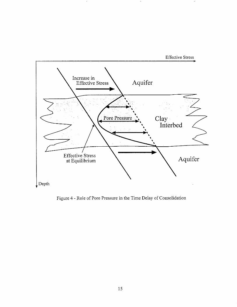
Figure 4 illustrates the role of pore pressure in the time delay of consolidation. The line
to the left represents the pressure in the aquifer system at a point of equilibrium before any
14
Effective Stress
Aquifer
~ -:~....~-. ' .
A~"""-·""'·""··"'""~"\04'-------1..=\""".t.
ClayInterbed
Effective Stressat Equilibrium
Depth
Figure 4 - Role of Pore Pressure in the Time Delay of Consolidation
15
Aquifer
change in stress occurs. As the effective stress in the aquifer increases, the low hydraulic
conductivity of the clay layer results in a parabolic profile of residual pore pressure. Complete
consolidation will not occur until all of the pore pressure dissipates and equilibrium is again
achieved.
There are two viable teclmiques for representing the time delay of consolidation. The
first is to consider the delay in the analytical derivation of the land subsidence model as illustated
by Shearer and Kitching (1994). In their Interbed Drainage Package (lOP), each model element
is split into two sub-elements; one for the coarse aquifer material and one for the fine-grained
interbeds. Flow between them is controlled by: (1) a parameter called vertical interbed
conductance, which is analogous to the conductance term in the stream-routing package of
MODFLOW (McDonald and Harbaugh, 1988); and (2) the head difference between the sub-
elements. Similarly, Leake's (1998, personal communication) IBS2 package allows for the
delayed release of water from compressible, discontinuous clay beds within an aquifer. However,
confining clay beds between aquifers must be simulated with individual model layers as they are
in the IBS 1 package (Wilson and Gorelick, 1996; Leake, 1998, personal communication).
The same result can be achieved numerically by dividing the larger low-conductivity
units vertically into a number of smaller units. The residual pore pressure is then represented
discretely across each compressible unit (Leake, 1990; Onta and Gupta, 1995). This second
approach has been employed in this model and allows for representation of the time delay using
the IBS 1 package. The actual implementation of this method will be discussed in further detail
in the following section.
It should be emphasized that the IBS 1 subsidence model only considers compaction due
to increased effective stress caused by changing ground water levels. It does not consider
16
subsidence due to hydrocompaction, withdrawal of gas and oil, deep-seated tectonic movement,
or the dewatering of organic soils. Of these alternative causes of subsidence, only
hydrocompaction has been significantly observed in the study area.
Hydrocompaction is subsidence that occurs as shallow, low-density soils are wetted for
the first time. In the Los Banos-Kettleman City area hydrocompaction has resulted from the
arrival of the California Aqueduct. Two sections of the California Aqueduct within the study
region, miles 98-103 and 114-129, appear to be especially sensitive to hydrocompaction. Water
was applied to these areas in the mid-1960s to exhaust the majority of hydrocompaction before
the aqueduct was constructed. It has been assumed that all significant hydrocompaction occurred
at that time and that it does not significantly contribute to subsidence during the modeling period
( 1972-2028).
3. APPLICATION OF THE MODEL
3.1 Modification of the Belitz et al. (1992) Model
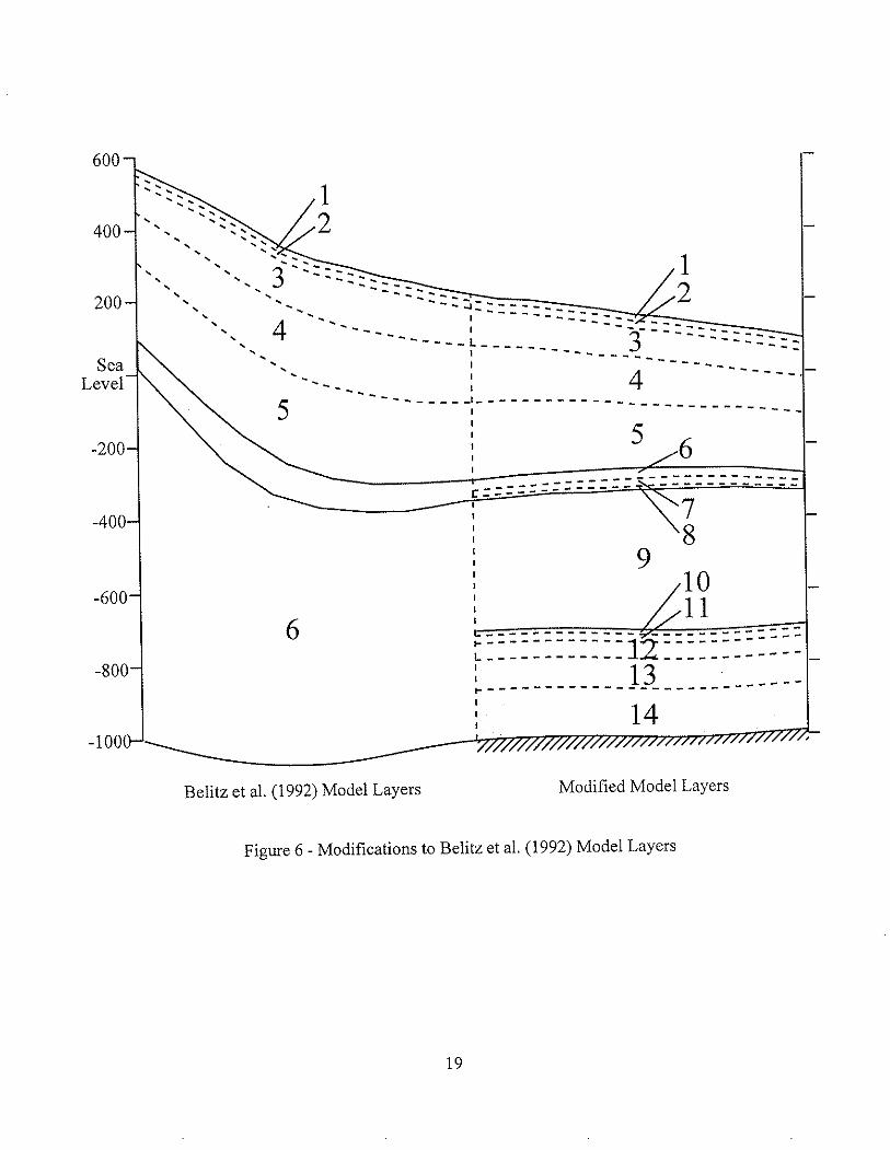
3.1.1 Geometry
The model used in this research is an adaptation of the Belitz et al. (1992) model.
Modifications have been made in order to simulate land subsidence due to ground water
withdrawal. No changes were made to the horizontal dimensions, model grid, and boundary
conditions as shown in Figure 5. Each grid cell represents a one-square-mile area with uniform
hydrologic and hydrogeologic parameters. The only significant change in geometry occurs in the
representation of the vertical model layers. Figure 6 shows the conceptual modifications made to
the Belitz et al. (1992) model. Most notably there is a change in how the low-conductivity layers
(the Corcoran clay layer and clay interbeds) are represented. In the Belitz et al. (1992) model,
17
[lJ Monitoring Wellwi0 extensometer
<%> Model Grid~ Boundary of c'(q,I/,~
, Valley Deposits ran. t:u-~ ::.r-'Study Area Boundary
o 5 10 MILESI iii I
o 5 10 KILOMETERS
Figure 5 - Model Grid and Location of Observation Wells
18
Five 0Points
SeaLevel
..... :: .•................•...... ... ....•. .. .... ... ..... .•. .... ... ...... .•. ...-, .••. .•...... 3 ::::-- ." " ...•.•. .••." " ~~::-- .•.•, , ~- ~~"" :-::-::-::--=--:::---~.,,~ --~::----..... 4 I ----::----
-. ---------~ ----::3----::::----" I--------~------- ----::....... , - -- - - •.....I 4 ----
_...... t-------~------------I --------------IIII
I
600
400
200
-200
5
-400
-600
6-800
Belitz et al. (1992) Model Layers Modified Model Layers
12
12
5 6
78
c========:::::--:::::::::::=
91011
~::::::::::::1-2-:::::::::::-L____________ ------------: 13 - --~-------------------------
14
Figure 6 - Modifications to Belitz et al. (1992) Model Layers
19
both the high-conductivity deposits as well as the clay interbeds in the confined aquifer system
have been represented as one composite unit. Additionally, the Corcoran clay layer has not been
directly included in the Belitz et al. (1992) model. Instead, its presence is accounted for by
reducing the vertical conductivity between layers 5 and 6. The model was satisfactory for
assessing the alternatives to agricultural drains, but is inadequate for modeling land subsidence.
In order to model subsidence, two maj or changes have been made regarding the
compressible, low-conductivity layers. First, the larger clay layers have been divided into
several smaller modeling layers. As discussed previously, this modification allows a head
gradient to develop between each clay modeling layer to mimic the presence of pore pressure
and capture the time delay of consolidation. The Corcoran layer is represented in this way. It
was divided into three modeling layers comprising 55, 30, and 15 percent of the layer thickness
(layers 6, 7, and 8, respectively). The thickness of the layers decreases with depth because the
largest head changes occur in the confined aquifer. As head in the aquifer changes, the steepest
head gradients in the Corcoran clay layer occur near the outer edge. The thinner layers are better
able to capture this gradient.
The Corcoran layer can be easily modeled this way because both its depth and thickness
are known. However, for the interbed layers of the confined aquifer, far less information is
available. Even if the location of each interbed was known, the large number of interbeds makes
modeling each separately a computationally impractical approach. The second major
modification to the model incorporates a possible solution to this problem suggested by Ireland
(1986). Instead of trying to map all the major interbeds in the confined aquifer, the interbeds are
removed from the confined layer and replaced by one large low-permeability layer at the bottom
of the aquifer.
20
This bottom layer is assumed to have a uniform thickness of 310 feet, located 1000 ft
below the Corcoran. It is divided into five modeling layers with thicknesses (for increasing
depth) of 10, 20, 40, 80, and 160 ft. There is a no-flow boundary at the bottom of the layer,
allowing drainage to occur only in the direction of the confined aquifer. Calibration will focus on
choosing parameters for the layer such that its effect on land subsidence is equivalent to the
composite effect of the actual interbeds.
The main limitation of the strategy is that since the bottom layer is an artificial
representation of the interbeds, characteristics of the layer such as storage coefficients (elastic
and inelastic) and vertical hydraulic conductivity cannot be verified by any field measurements.
This means the validity of the layer parameters can only be measured by their ability to predict
subsidence.
3.1.2 Pumping
The other major modification to the Belitz et al. (1992) model occurs in the
representation of ground water pumping. The pumping of ground water from the aquifer system
is one of the most important components of the ground water model, affecting piezometric head
in the confined aquifer more than any other single variable. It is also one of the most difficult
components to model because it has never been directly measured.
The Belitz et aL (1992) model estimated pumping magnitudes using the same nme
subareas designated in the water budget by Gronberg and Belitz (1992). Pumping rates are
allowed to vary between subareas, but are uniform within each subarea. Well depths and
perforation lengths were used to determine the percentage of pumping from upper and lower
water-bearing units. The 1980 water budget values (Gronberg and Belitz, 1992) were adopted
for all model years.
21
This model adopts the spatial distribution of pumping in the Belitz et al. (1992) model,
but alters the yearly magnitude estimates. The major limitation of Belitz et al. (1992) approach
is that the magnitude of pumping for all model years was assumed to be exactly the same. This
was satisfactory for the purposes of their report (Belitz et al., 1992; Belitz and Phillips, 1995),
but does not capture the pore pressure fluctuation necessary to model land subsidence.
There are two major sources of water in the Las Banos-Kettleman City region, surface
water from the CVP and ground water. Although ground water pumping has not been measured,
some records of water delivery from the CVP are available. Records from the Westlands and
Panoche Water Districts are summarized in Table 2. These rates have been used to construct an
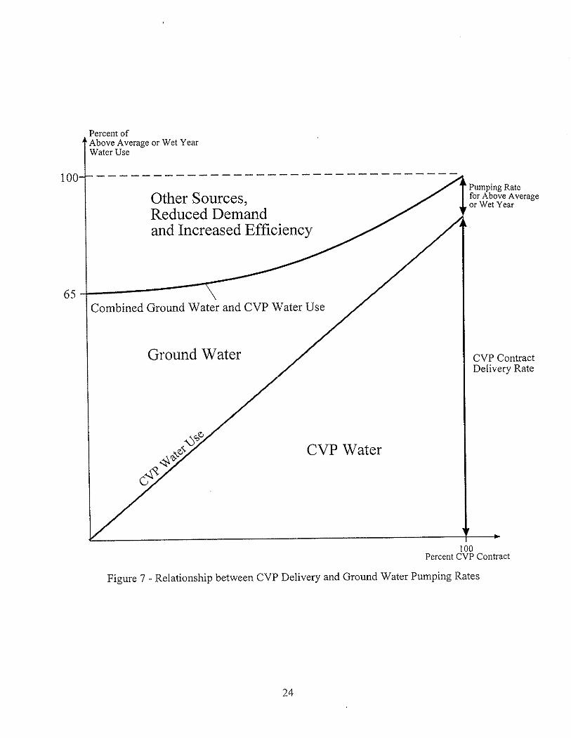
estimation of the pumping rate for each model year. Figure 7 illustrates the relationship adopted
between CVP water delivery and ground water pumping rates.
Several assumptions have been made in creating this figure. First, it is assumed that the
Gronberg and Belitz (1992) water budget is appropriate for years in which 100 percent of the
CVP contract water is available. During years of reduced surface water availability, the shortage
can be met by reducing demand (land retirement), increasing irrigation efficiency, procuring
other sources, or increasing ground water pumping. The line of combined ground water and
CVP water use is assumed to be concave up. This is because increasing efficiency and the use of
other sources are inexpensive alternatives for years with small reductions in CVP water. For
increasing levels of drought, however, these options become very costly or unavailable. Thus, an
increasing amount of the shortage must be met with ground water. The actual shape of the line
of combined ground water and CVP water use was determined through trial and error
22
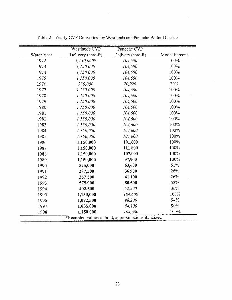
Table 2 - Yearly CVP Deliveries for Westlands and Panache Water Districts
Water YearWestlands CVP Panoche CVPDelivery (acre-ft) Delivery (acre-ft) Model Percent
197219731974197519761977197819791980198119821983198419851986198719881989199019911992199319941995199619971998
1,150,000* 10{6001,150,000 104,6001,150,000 104,6001,150,000 104,600230,000 20,920
1,150,000 104,6001,150,000 104,6001,150,000 104,6001,150, 000 104,6001,150,000 104,6001,150,000 104,6001,150,000 104,6001,150,000 104,6001,150,000 104,6001,150,000 101,6001,150,000 111,8001,150,000 107,0001,150,000 97,900575,000 63,600287,500 36,900287,500 41,100575,000 80,500402,500 52,500
1,150,000 104,6001,092,500 98,2001,035,000 94,1001,150,000 104,600
100%100%100%100%20%100%100%100%100%100%100%100%100%100%100%100%100%100%51%26%26%52%36%100%94%90%100%
*Recorded values in bold, approximations italicized
23
Percent ofAbove Average or Wet YearWater Use
65-1------"\
----------------------------------100
Other Sources,Reduced Demandand Increased Efficiency
Pumping Rate .for Above Averageor Wet Year
Combined Ground Water and CVP Water Use
Ground Water cvr ContractDelivery Rate
CVP Water
100Percent CVP Contract
Figure 7 - Relationship between CVP Delivery and Ground Water Pumping Rates
24
during the model calibration and can be mathematically described as:
(4)
in which (/Jc is the percent of normal, combined ground water and surface water use; and CPs is
the percent of contracted surface water.
This relationship not only assures consistent estimation of pumping rates for the
calibration period, but also provides an estimate for future pumping rates based on the
availability of surface water.
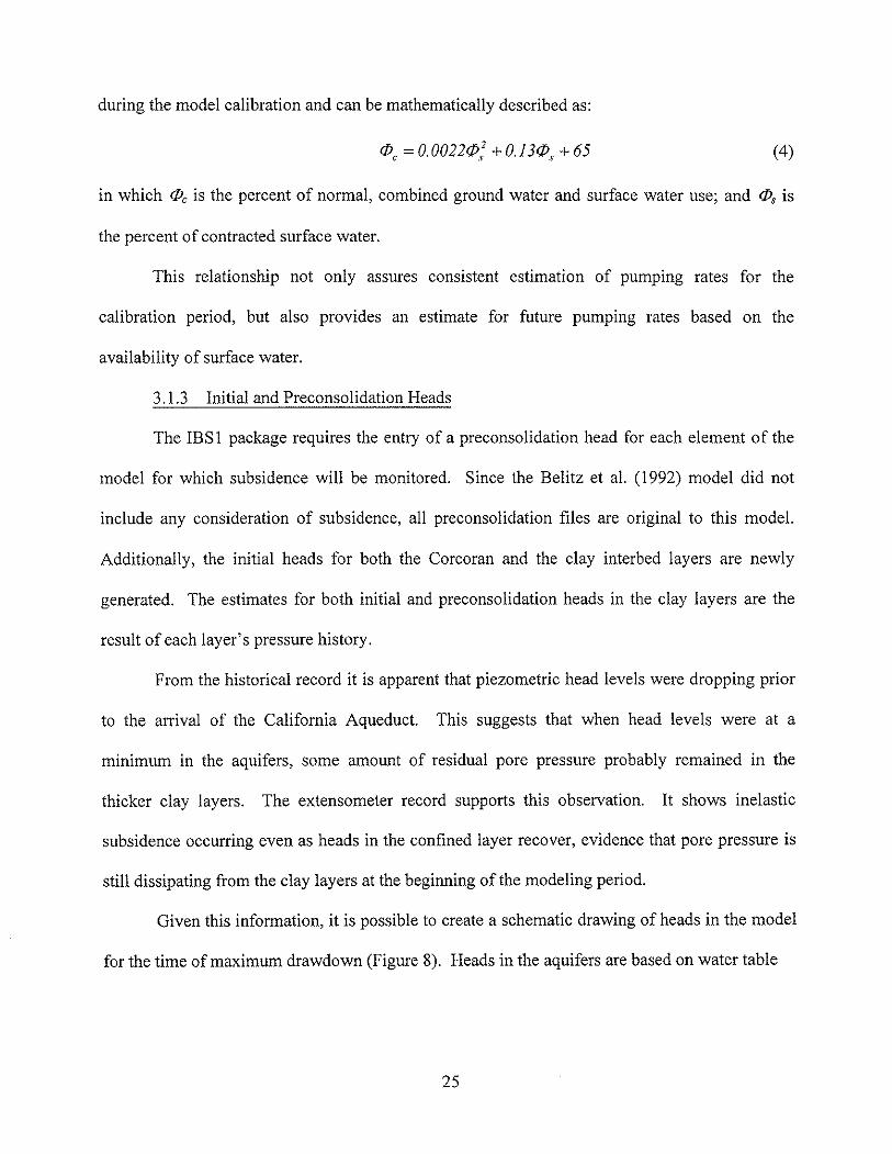
3.1.3 Initial and Preconsolidation Heads
The IBS 1 package requires the entry of a preconsolidation head for each element of the
model for which subsidence will be monitored. Since the Belitz et al. (1992) model did not
include any consideration of subsidence, all preconsolidation files are original to this model.
Additionally, the initial heads for both the Corcoran and the clay interbed layers are newly
generated. The estimates for both initial and preconsolidation heads in the clay layers are the
result of each layer's pressure history.
From the historical record it is apparent that piezometric head levels were dropping prior
to the arrival of the California Aqueduct. This suggests that when head levels were at a
minimum in the aquifers, some amount of residual pore pressure probably remained in the
thicker clay layers. The extensometer record supports this observation. It shows inelastic
subsidence occurring even as heads in the confined layer recover, evidence that pore pressure is
still dissipating from the clay layers at the beginning of the modeling period.
Given this information, it is possible to create a schematic drawing of heads in the model
for the time of maximum drawdown (Figure 8). Heads in the aquifers are based on water table
25
Piezometric Head
Unconfined Aquifer
.A;
;,,.;, .. ,
". i; ., /------------;~-- 1-----------------, .i/ Corcoran Clay Layer
-~t-------------------.;,--------4--.,
.;
· Initial piezometric head·I
Upperjbound for pre-consolidation head
Confined Aquifer ~I·
Equilibriumlpiezometric head· Residual pore pressure·1---------------------- -- -r---------------------I------ ---- --.-----------------------
I:.••••••• __ "--~ ! Interbed Layer______ L~~ ~~-~---~-------~-~--~-II
.. ·.1··.· ...... ... . ......... . ... . .... .... ......1lI111l11111111111111111111l1l11l11ll1U11I11I11I11I1II1ll1l1I1I1II11I1II1II1ll1ll11II1I II 111III 1III III 111111111111111II III 11III 11111111111111111111111111111111111111III 111111III 11111111111111111111111111111111
Depth No Flow Boundary
-------,.---
Figure 8 - Schematic Drawing of Initial Heads
26
and potentiometric surface maps from 1972 (after Belitz et aI., 1992). Heads in the low-
conductivity layers will be equal to the equilibrium piezometric head plus the residual pore
pressure. The equilibrium head is determined from the initial heads in each aquifer. The shape of
the residual pore pressure profile is assumed to be parabolic. The magnitude of the residual pore
pressure will be a function of past changes in piezometric head and the thickness and hydraulic
conductivity of the clay layers. Since this information is unknown, the magnitude of residual
pore pressure is treated as a calibration parameter.
Because of the relatively small changes in the water table, only residual pore pressure
from changes in piezometric head in the confined aquifer is considered. Additionally, Figure 8
shows the upper bound for pore pressure being equivalent for both the Corcoran and interbed
layer. This is not necessarily true. The rate at which each fine-grained geological unit will
dissipate pore pressure will be a function of its thickness and hydraulic conductivity. Even
though the pressure history for the confined aquifer is the same for both the Corcoran and the
interbed layers, the amount of pore pressure remaining from these changes need not be equal.
For this model, the best results were produced with residual pore pressure being two times
greater in the interbed layer than in the Corcoran.
The above observations are only applicable for the time of maximum drawdown. The
time of maximum drawdown is also a convenient time period to consider head levels because
initial and preconsolidation heads will be equal to each other. For this reason, it is assumed that
the initial heads for the model are equal to the maximum historical drawdown. Although some
amount of recovery has occurred between the arrival of the aqueduct (approximately 1967) and
the beginning of the model (1972), the initial heads in the confined aquifer are sufficiently close
to the historic minimum for this assumption to produce acceptable results. Additionally, the
27
assumption affects only the outermost portions of the Corcoran and clay interbed layers,
resulting in minimal effect to overall land subsidence.
Finally, initial heads in the aquifers remain largely unchanged from the Belitz et al.
(1992) modeL Modifications were made only where large jumps were observed in the initial
time steps indicating that the head values were inconsistent with the rest of the model. This was
particularly prevalent in the bottom layer of the unconfined aquifer (Belitz and Phillips, 1995).
Such inconsistencies usually stabilize in the first few time steps. Although they have little effect
on the long-term accuracy of the ground water flow portion of the model, they cause large
fictional jumps in land subsidence. For this reason, model head values for the bottom layer of
the unconfined aquifer were chosen after four time steps (1974) in the generation of initial and
pre-consolidation heads in the Corcoran clay layer. This allowed sufficient time for any transient
instability to dissipate. A small number of other changes to initial head in the aquifers occurred
near the edges of the model grid, but were not aerially extensive.
3.1.4 Other Modifications
All other aspects of the model have not been significantly changed from the model
developed by Belitz et al. (1992). For information on the selection of parameters for drainage,
evapotranspiration, recharge processes, and boundary conditions, the reader should consult
Phillips and Belitz (1991), Belitz et al. (1992), and Belitz and Phillips (1995).
As in the Belitz et al. (1992) model, the model formulated in this study uses yearly stress
periods. This has been done because most of the data (water table levels, subsidence rates, CVP
deliveries, etc.) are only available at yearly intervals. The major weakness of this approach is its
effect on pumping. By averaging the pumping out over the entire year, the higher drawdowns
occurring during the summer months are lost. This is significant for the land subsidence portion
28
of the model because most of the subsidence actually occurs during these periods of high
drawdown. This can be compensated for by altering some of the other model parameters, but it
should be noted that the piezometric heads predicted by the model will be artificially high during
the summer months.
It should also be noted that, in addition to the temporal averaging of pumping rates,
pumping is also averaged spatially over the grid cells. During calibration, measured ground
water levels were assigned to the center of the grid cells and compared with the spatially and
temporally averaged model-computed ground water levels. In short, although spatial and
temporal averaging of parameters causes the loss of some information, it is unavoidable in
numerical modeling efforts, mainly due to the scarcity of data and/or budget and time restrictions
for more detailed data gathering.
3.2 Calibration
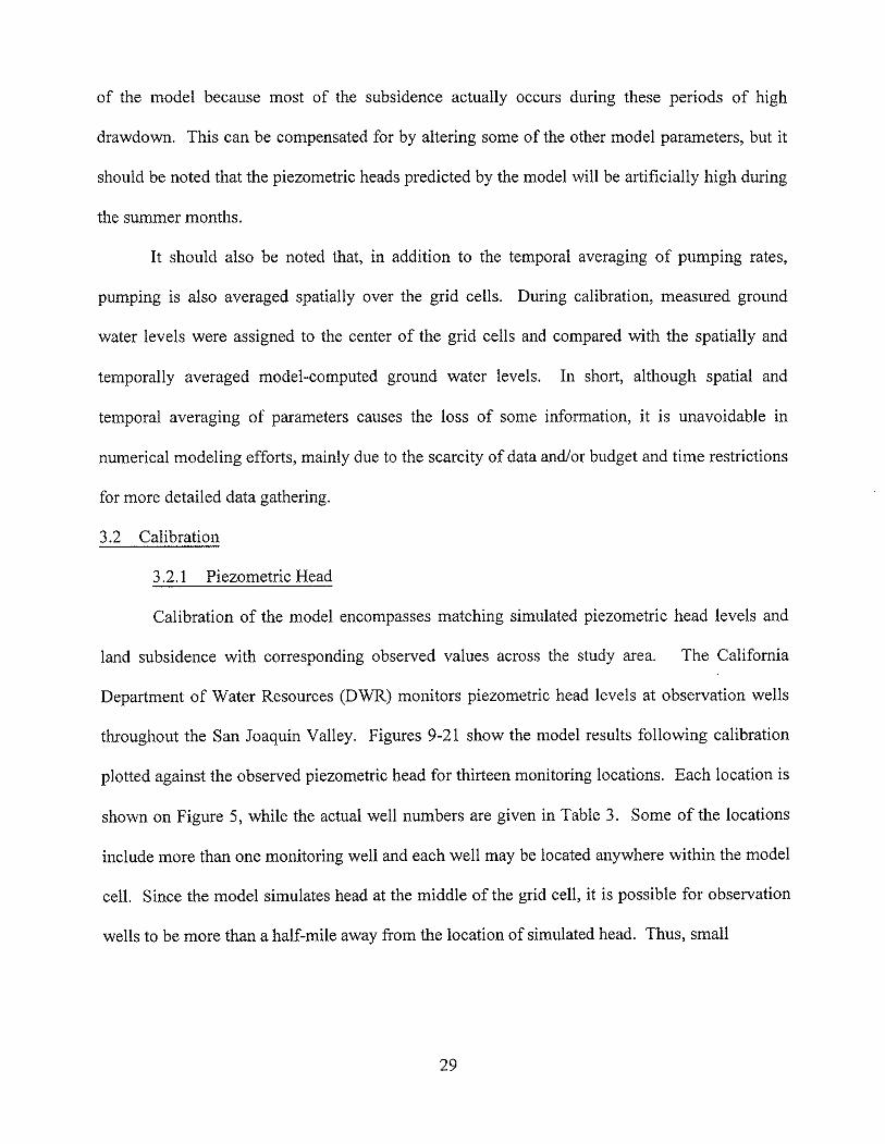
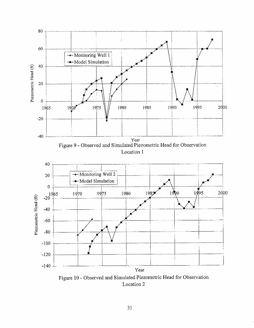
3.2.1 Piezometric Head
Calibration of the model encompasses matching simulated piezometric head levels and
land subsidence with corresponding observed values across the study area. The California
Department of Water Resources (DWR) monitors piezometric head levels at observation wells
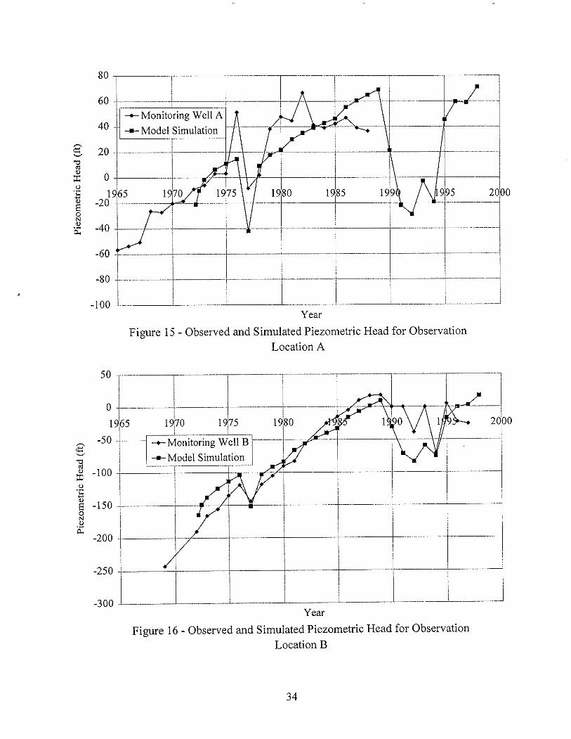
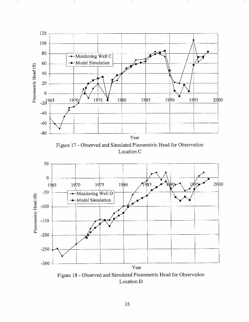
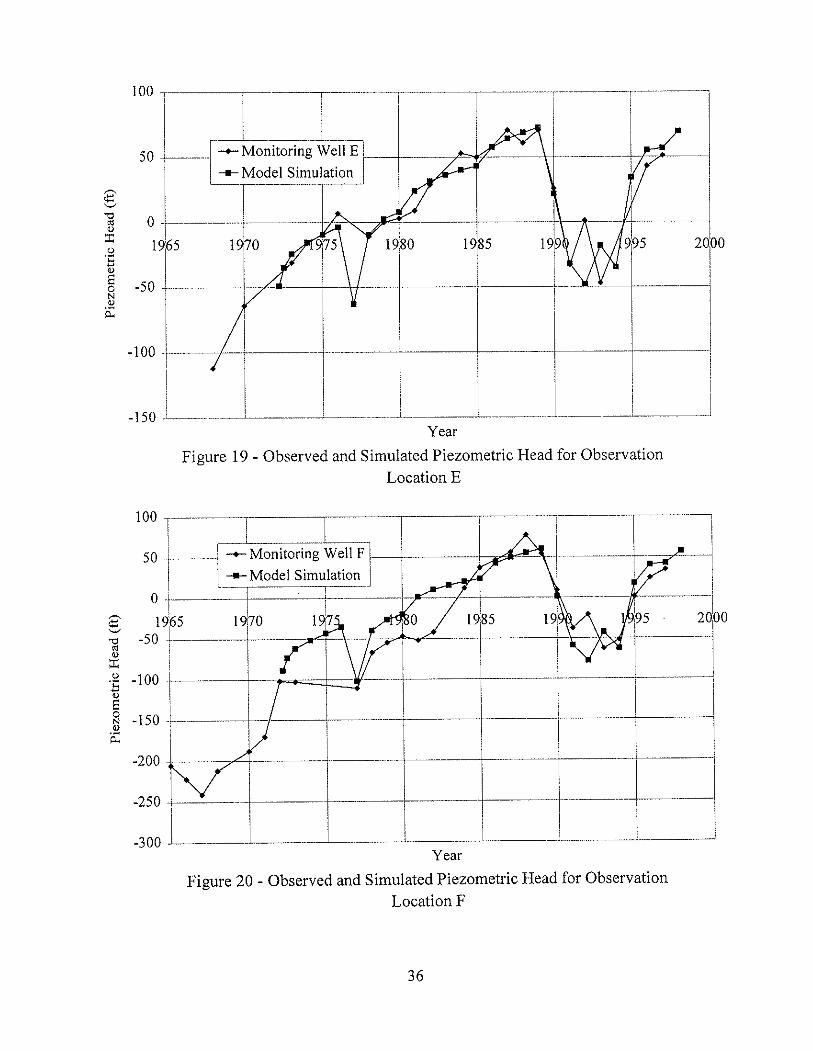
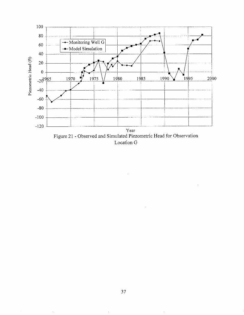
throughout the San Joaquin Valley. Figures 9-21 show the model results following calibration
plotted against the observed piezometric head for thirteen monitoring locations. Each location is
shown on Figure 5, while the actual well numbers are given in Table 3. Some of the locations
include more than one monitoring well and each well may be located anywhere within the model
cell. Since the model simulates head at the middle of the grid cell, it is possible for observation
wells to be more than a half-mile away from the location of simulated head. Thus, small
29
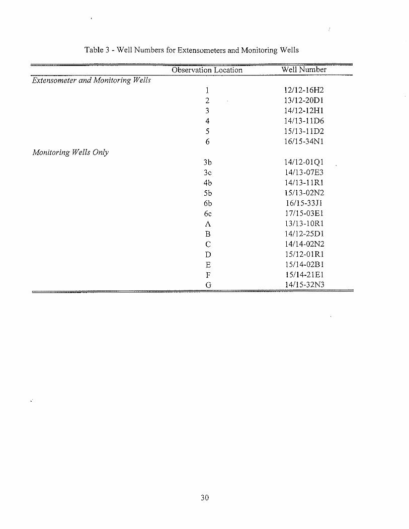
Table 3 - Well Numbers for Extensometers and Monitoring Wells
Observation Location Well NumberExtensometer and Monitoring Wells
123456
12112-l6H213/l2-20Dll4112-l2Hl14113-11D615113-l1D216115-34Nl
Monitoring Wells Only3b3c4b5b6b6cABCDEFG
14/12-01Ql14/13-07E314113-l1RI15113-02N216115-33J117/15-03El13/13-10RI14112-25Dl14114-02N215112-01Rl15/14-02B 115114-21El14/15-32N3
30
i::l _I~MO~el~f-1~_J f-I_~=1--~J~ I i I I I ' . I
£ ~L--l~~ - 1 ~185 If---t---1Iii I I-2°1 -I --·-··~·~~II--·-·--I--···-I---~-l-·----I ' I iii I
-40 i l. . L__. I I i ._... _.~ ..~Year
Figure 9 - Observed and Simulated Piezometric Head for ObservationLocation 1
YearFigure 10 - Observed and Simulated Piezometric Head for Observation
Location 2
31

-300 -'----Year
Figure 11 - Observed and Simulated Piezometric Head for ObservationLocation 3
Year
Figure 12 - Observed and Simulated Piezometric Head for ObservationLocation 4
32
Year
Figure 13 - Observed and Simulated Piezometric Head for ObservationLocation 5
150 r-·~· I n I I I I ---II r--M· .. W 116al-----1 I I
100 -~I\ ~I=::M~~:i~~i~~W:ll ~~ I -I .- ·-:-_·_-·_\-/-_·-······150 I i -- Monitoring Well 6c i I " Il·-~ --- Model Simulation J 'I T- 0 .--.-~- --
2' 0 _1_._L. -~ --1=-~_... ~ L ._~_ i - -j!_sJ9~_ lr__l~1+~:8S _ lr~~rs-- 20eO
~.:l ~1=---=-ft--- ., e- -~-2ool-~-.- --- ~ I n I _. I .-I-~--~::::~I~ t \_ ±- 1_-
0
-----1
YearFigure 14 - Observed and Simulated Piezometric Head for Observation
Location 6
33
, ~- ~~--
;~~5 19~-~95 -jOOI --f ~ ~~i---~-'--
---.-~---+-- I ---1~~'--"'----~--+-~~. 1--- I --- .... 1i i
! Ii!.~~.~---+-- -,-:--------l~~~-r·---l~~ __ _____LI _~ 1 ~_1 _._,
"[-·----1I ~'~I -.--!
1~80
YearFigure 15 - Observed and Simulated Piezometric Head for Observation
Location A
YearFigure 16 - Observed and Simulated Piezometric Head for Observation
Location B
34
Year
Figure 17 - Observed and Simulated Piezometric Head for ObservationLocation C
50 I 1.. T--I. I_------i---lo -j 'j T·· I 1- ... ui· ·-t---j19
1
65 19[10 1(f5 1180 9185 ,9 1 ~ 2°100
g -50 -~ --Monitori.ng W~llDr---+-'-' --1-- !. --·I"-,--_···-··j""g ! i -- Model SImulatIon I I / I I ! I~ -I001--! - --1-----
1----t--"'-I
S -150 "f.-.---. --, - - ._L __._~_, __-.l, I~ I I I I I
-200r-~ i ~~ 1 I -1-250 .·.n_ 4 --l] I 1 -1-300 ..L I L... _.1 L..~_J
Year
Figure 18 - Observed and Simulated Piezometric Head for ObservationLocation D
35
-100 T'__ ~I-_l._--_-~-..-._~-i II Ii I I-150 .L-__,.~~~ .__. -'----
Year
Figure 19 - Observed and Simulated Piezometric Head for ObservationLocation E
Year
Figure 20 - Observed and Simulated Piezometric Head for ObservationLocation F
36
100 T I ---.-T.-.--------·--~[-m---~-l-·--· ....-·--I80 ·+-----b i i I~:::::~LL_ .-~~.--
60 -I I--Monitoring Well G --1._.1 --- i -----1
I --- Model S~~lUlation! I- I
40 I ..---.--- I :-"--~I--~-II I . .. I i
~v::r::o.c:ti
~ I I I I i Iv AO.. -'"", ---'---1 i -+-
i !i Ii --.-.--~ ~--100 --- . I -t-- I I
-120 I ,___ ___! ! ! .J .J
YearFigure 21 - Observed and Simulated Piezometric Head for Observation
Location G
37
differences should be expected between observed and simulated piezometric head values, as well
as between head values at different observation wells within the same grid cell.
By using the aquifer parameters found by Belitz et al. (1992), it was possible to produce
relatively accurate results for piezometric head with modification to the pumping rates only.
Proper drawdown during years of drought was achieved using the scheme described in Section
3.1.2. In addition to determining the best equation to define combined ground water and surface
water use (see equation 4), the calibration dictated two other significant changes.
The water budget for the Belitz et al (1992) model includes a portion of the Westlands
Water District that relies strictly on ground water. Following construction of the water budget,
however, improvements were made in the delivery system to bring CVP water to portions of this
area. This was evident during the calibration trials when predicted head levels were significantly
below those observed in these portions of the Westlands Water District. To address this
problem, the original water budget is retained for the model years up to 1980, but it is assumed
that CVP water replaces 25 percent of the pumping in 1981 and replaces 50 percent in 1986.
The second significant change to the pumping scheme occurs along the southern edge of
the study area. Observed head values suggest that more ground water is removed from this area
during periods of drought than predicted by the model. By increasing the pumping 150 percent
during periods of drought, the head levels in the model appear to better match the observed data
in the region.
3.2.2 Land Subsidence
Land subsidence in the San Joaquin Valley has been documented usmg both
extenso meters located at wells throughout the Valley and level runs along the California
Aqueduct. Extensometers provide the most detailed measurement of compaction. Annual
38
extenso meter measurements can be plotted directly versus model predictions. Unfortunately,
each extensometer only records subsidence at one point, and only six are located in the study
area. Level runs provide a better indication of subsidence trends spatially. Although they are
conducted only once every four years, they measure subsidence along a path line.
The six extensometers included in this study (Figure 5) were installed by the U.S.
Geological Survey (USGS) and are now monitored by the San Joaquin district of the California
DWR. Three of the extensometers were abandoned in the 1970s and thus provide only a partial
record for the calibration period. For those extensometers that continue through the entire time
interval (l972~ 1998), a small portion of the data is missing from the record (1979-1984).
Fortunately, the missing portion corresponds to a time of relatively uniform rebound. For this
portion, rebound is assumed at a rate equal to the average of the rebound in the years 1978 and
1985.
Extensometers only measure compaction across a monitored depth. As a result,
additional compaction can occur below the monitored interval and surface subsidence will
usually be greater than the compaction measured by the extensometer. Compaction is
tranformed to subsidence by multiplying the observed compaction by the average ratio of
subsidence to compaction found for each extenso meter (Ireland et al., 1984). Figures 22-27
show the model results following calibration plotted directly against the transformed
extensometer data.
Extensive level runs were conducted for the Los Banos-Kettleman City region throughout
the 1950s and 1960s. Although more recent data could not be accessed for this project, the
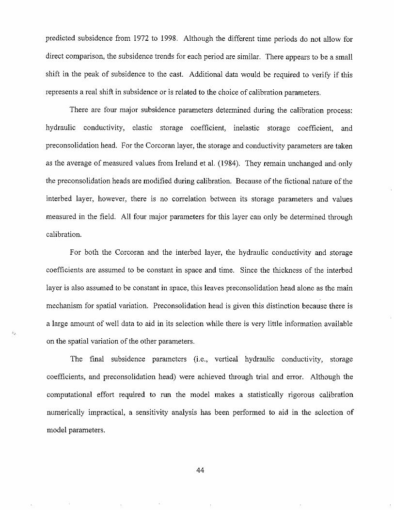
previous level runs give a good indication of subsidence trends for the area. Figure 28(a) is a
contour map of the measured subsidence from 1926 to 1972, while Figure 28(b) shows the
39
7511-~~-'I--il-i~-"=r -···-··-·····--:~~----I1 1 l ~ !
g 71 -I -.---r-----~-I ! -I ~~t--~~~lg6.5 ~~-- l----~ll~ -~ II -+--1~ I l i I ! I
~ 6~-~-t t--'---'-"--~i-~ II~Alt~iV~ AGII I I ~ i -- Alternat~ve B I ~i
5.5 _I - ... ---~ I ! . ._----1__-+- AlternatIve C ~-!
I I i I!
5 ~ .- ,--- --~.------~-- ... --~f ~
1998 2003 2008 2013 2018 2023 2028 2033Year
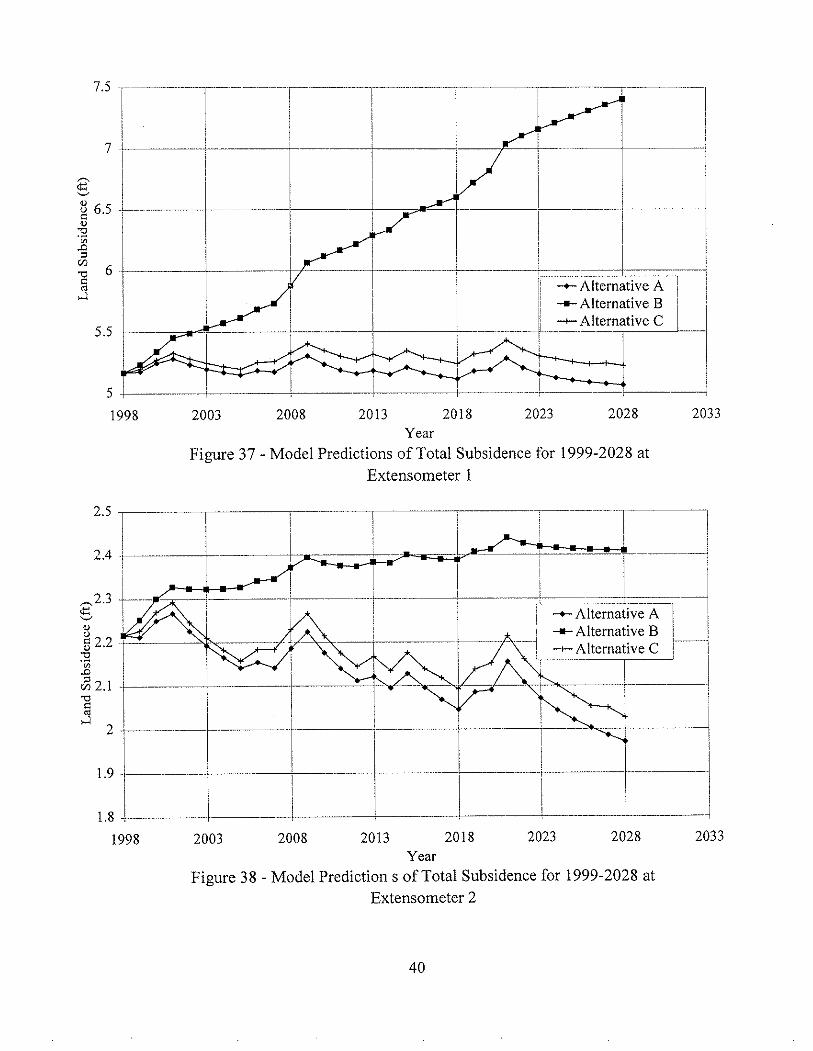
Figure 37 - Model Predictions of Total Subsidence for 1999-2028 atExtensometer 1
2.51,----- -·---l---------l 1
2.4 -f-~--- 1 i ---~------.---!g231--- L---f- I --~'=~~b,-I8 iii -- Alternative B I I~ 2.2 1- .------ - t------·r--·· -'--1 -+- Alternative C I"---j~ i' I-:"'---'---~ I~ 21r! __ -L~········~~·JI--- -. -T- -----·r-~---l5 I . I I i !
2 --; --- ..._._- _. ~---
191~-· --------+--
1.8 J---.-.. i ---f.-. : 1--1998 2003 2008 2013 2018 2023 2028 2033
YearFigure 38 - Model Prediction S of Total Subsidence for 1999-2028 at
Extensometer 2
40
4.6l=r~~I------1------1 r-------~I------:44 f ·-i-r- r 1-, -t- .'
g 4.2 -r---\- -.I T-- I --~. ----- i -1o 4 .j..... , -, .~ I--1-- ...J] I I I .~I II --Alternative A I.~ 3 8 ~- . --L- -----11 .- ... ---J. -----Alternative B L_j.g . ! I i I II -+- Alternative C i I~ ~ iii L-._____ I .~ Ij 3.6· ··--I-~--I------I~-I
3.4 -~-.. - 'I --- , --I -I-l32 f-- I -1- ,---T I3 ., -~-~- ! ----l ! -1-._ ..- :1998 2003 2008 2013 2018 2023 2028 2033
YearFigure 39 - Model Predictions of Total Subsidence for 1999-2028 at
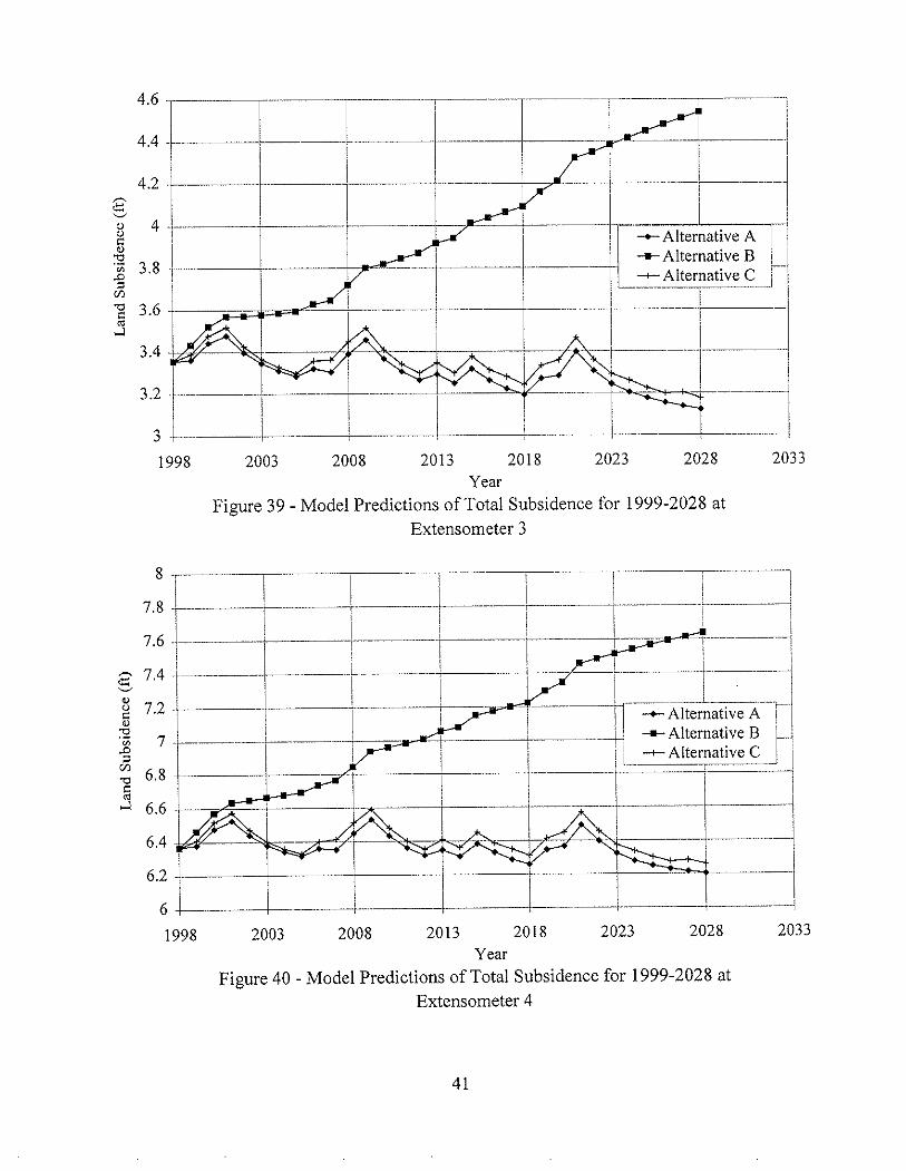
Extensometer 3
7:~---L l_ L------L-~=-J..~~~!-·--·~~7.6 -1 I l------.--r----i -+__ I
~ 741 I---r l----i-- -r t--· ---·-1g 7.2 ··-1" - L_. I i - -1----··-·_-- 1'1'· --Alternative A--r-.il,.g I Iii I
~ 7 -~'. ---I _.__ ..n i i i ----Ito. =:~~~~~~--Jl-g 6.8 --+-------r---- I I -_._[ I-i{';j • ! I I i.....Jo 6.6 - - :-- .- .-._\ 1 ·1 ··---~-·-l
6.4 - _.,-- " -I6.d 1 I =c ·16 .1 ~ .. -------+-- .--l.. --I
1998 2003 2008 2013 2018 2023 2028 2033Year
Figure 40 - Model Predictions of Total Subsidence for 1999-2028 atExtensometer 4
41
2008 2013 2018 2023 2028 2033Year
Figure 41 - Model Predictions of Total Subsidence for 1999-2028 atExtensometer 5
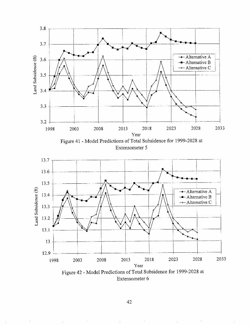
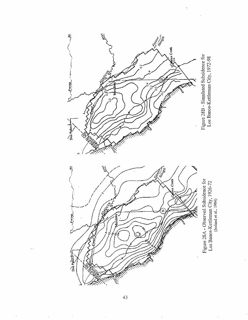
1998 2003 2008 2013 2018 2023 2028 2033Year
Figure 42 - Model Predictions of Total Subsidence for 1999-2028 atExtensometer 6
42
»>.•.£!~.~1J9--."-i-"''--....r:
:---
-----'..-
-8i )
{.
\ \.<,
<,'..: -, <,<,
~ w
Figure
28A-O
bservedSubsidence
for
LosBanos-Kettleman
City,1926-72
(Ireland
etal.,1984)
;..
...-£!~!'!9--..,--
...~"'./
···-----..···--8f)
.s->
Figure
28B-S
imulated
Subsidence
for
LosBanos-Kettleman
City,1972-98
...4~ "':'···<S'-Q
oS?
o:-':
":".
~.q
'....
predicted subsidence from 1972 to 1998. Although the different time periods do not allow for
direct comparison, the subsidence trends for each period are similar. There appears to be a small
shift in the peak of subsidence to the east. Additional data would be required to verify if this
represents a real shift in subsidence or is related to the choice of calibration parameters.
There are four major subsidence parameters determined during the calibration process:
hydraulic conductivity, elastic storage coefficient, inelastic storage coefficient, and
preconsolidation head. For the Corcoran layer, the storage and conductivity parameters are taken
as the average of measured values from Ireland et al. (1984). They remain unchanged and only
the preconsolidation heads are modified during calibration. Because of the fictional nature of the
interbed layer, however, there is no correlation between its storage parameters and values
measured in the field. All four major parameters for this layer can only be determined through
calibration.
For both the Corcoran and the interbed layer, the hydraulic conductivity and storage
coefficients are assumed to be constant in space and time. Since the thickness of the interbed
layer is also assumed to be constant in space, this leaves preconsolidation head alone as the main
mechanism for spatial variation. Preconsolidation head is given this distinction because there is
a large amount of well data to aid in its selection while there is very little information available
on the spatial variation of the other parameters.
The final subsidence parameters (i.e., vertical hydraulic conductivity, storage
coefficients, and preconsolidation head) were achieved through trial and error. Although the
computational effort required to run the model makes a statistically rigorous calibration
numerically impractical, a sensitivity analysis has been performed to aid in the selection of
model parameters.
44
3.3 Sensitivity Analysis
3.3.1 Hydraulic Conductivity
Hydraulic conductivity is represented in two directions, vertical and horizontal. The
horizontal conductivity is of little interest in the interbed layers because small head gradients and
long flow paths result in insignificant horizontal flow. Additionally, the horizontal flow should
not be significantly changed by the new model arrangement. Hence, it is acceptable to adopt the
average horizontal hydraulic conductivity in the interbed layers as measured in the field by
Ireland et al. (1984).
Conversely, the vertical conductivity greatly affects the performance of the model. It
determines the rate pore pressure leaves the fine-grained layers and hence, the rate of subsidence.
Figure 29(a)-(f) shows the model results obtained using fourfold and one-forth of the calibrated
hydraulic conductivity values. As predicted, the rate of consolidation is very dependent upon the
hydraulic conductivity while the general trend of the subsidence is not greatly affected.
3.3.2 Elastic and Inelastic Storage Coefficients
The elastic and inelastic storage coefficients determine the magnitude of subsidence for a
given change in hydraulic head. The elastic coefficient can be examined independently of the
inelastic coefficient during periods of rebound. The small volume of water flowing from the
low-conductivity layers during elastic compaction means there is much less time delay
associated with rebound than with consolidation. Hence, the rate of subsidence during rebound
is almost exclusively determined by the elastic storage coefficient. This makes the elastic
coefficient the easiest parameter to calibrate because it can be chosen, virtually independent of
the other parameters, to match the observed rebound rate.
45
5.5,.. I '-1 -~ --'--I"-~5.r-+------; --'1 " ..---I -.~-
4.5 y--.---+---+.-r; ..-- ~--- ~-§: 4f-_.~~_-L '-=c=1 r--I ---t--------is I i 1 ! I I Ij 3: F-··=t~-]------'- C J ..::J::j] 2.5 t-"--i ~~-~ r----'i... Observed sUbsrd-inc~-1
2+-~·--t'~~t---,-----Jl
400% Vert. Hydraulic Conductivity\-LSt--- ._..__~' I _ .-25% Vert. Hydraulic Conductivity II i r- .....Filial Calibration ._ ..__1 -r- ~... I ~ ] ---, .. ·-··--~i
1960 1965 1970 1975 1980 1985 1990 1995 2000Year
C • Extensometer 3
YearE - Extensometer 5
s"u""'tl.;;;"" 5.5~'"-e§
5-'4.5
1980Year
D - Extensometer 4
1990 20001975 1%5 1995
,~:tf-~=-~i--!-::--!~~=-n€ 13.51---t.--.--+---~-.- ...." : _-1. -- ..,-~--j~ 13 ._.~J~~ ! 0. • •• '.... c.' --'" ~
.g I Ii,! I Ei~ 12;~r==p--l L-r. ·---·~.i~---..'"j.- --l--Jt=--==,-~a 115 1-..- ! I ,.1 -..-'----,-. ----.-'--~ !-' . I . -- ;._-.----, -l- Observed Subsidence ~1
11 .f-.--!--- -l---~----·l..•...400% Vert. Hydraulic Conductivit i105 .1 .L_ I __ L ..__ j ..•...25% Vert. Hydraulic Conductivity i__10CLI Ls=Final C_~lib~'!.i~~_i_ '"l~-~I
1960 1965 1970 1975 1980 1985 1990 1995 20QOYear
F - Extensometer 6
Figure 29A-F - Simulated Subsidence for 400, 100 and 25 Percent of Final Calibrated Value ofVertical Hydraulic Conductivity at Six Extensometer Locations
46
The contribution of the inelastic coefficient is much more difficult to isolate. It has the
least visible effect on the performance of the model, During inelastic compaction a significant
volume of water is expelled from the compressible model layers. Because the rate of this
expulsion is governed by the vertical hydraulic conductivity, the rate of inelastic consolidation is
dominated by the vertical conductivity, not the inelastic storage coefficient. Instead, the latter
coefficient determines how quickly the preconsolidation head falls in each layer as consolidation
occurs. Thus, it is an important parameter in determining when inelastic compression starts and
stops. Figures 30(a)-(t) show the model results obtained using fourfold and one-forth of the
calibrated elastic storage coefficients, while Figures 31(a)-(t) present the same information for
inelastic storage coefficients.
3.3.3 Preconsolidation Heads
The preconsolidation heads for the Corcoran and interbed layers are determined using the
process described earlier (section 3.1.3). Grids of the final preconsolidation heads for each layer
can be found in the appendix of this report. If a parabolic profile is assumed as shown in Figure
8, only the upper bound of residual pore pressure need be determined through calibration. This
upper bound of residual pore pressure was first approximated using the 1943 head values in the
confined aquifer. The year 1943 was chosen because it was approximately this time when intense
ground water withdrawal began to cause the most serious subsidence. These values were then
adjusted during the calibration process to match observed subsidence.
Preconsolidation head has two effects on the modeL First, an increase in
preconsolidation head (and corresponding increase in initial head) results in an increased rate of
subsidence because of the larger gradient between heads in the aquifers and in the compressible
layers. Second, an increase in preconsolidation head results in longer periods of subsidence
47
g':~1 J -f 7IJ ~i 4.5 'Ft .L 1--i'~~ ,- ---1! 4 . --+~~- ~ --J~.~-+-I-!-----1] -l4 1"-'-::;::Ob-;~~CdTubSidenCe
3.5 [ _11'400% Elastic Coefficient __ II ..•...25% Elastic Coefficient ,
3 l- _L_m I .-i ~.i.~~~~On ---J1960 1965 1970 1975 1980 1985 1990 1995 2000
YearA • Extensometer 1
,:~- ---.~
i 3 r-'- i ,. --I-~fj 2':~'..~*7r=,,-I_oJ::'Llll~
~ I 1 ..••.. 400% Elastic Coefficient1 5 -. - I --H, --25% Elastic Coefficient I-
I I . . I1 I -- Final Callbration j 1
I +- .._*---1-- I T"~ - l=====·~i1960 1965 1970 1975 1980 1985 1990 1995 2000
YearC • Extensometer 3
Ii.+__~L_.~_--+_: I I- Observed Subsidence..••..400% Elastic Coefficient--.!l- 25% Elastic Coefficient..•...Filial Calibration
1960 1970 1975 1980 1985 1990 1995Year
E - Extensorneter 5
1965
,:FP=!iJ-T~-=JI,~ --I-f-r'-.~.--==<ct------1i':t- i ·li_m~!=~L-~~I....l I - Observed Subsidence
. I .. I ..•..400% Elastic Coefficient0.5 - r'" - --l'-I 25% Elastic Coefficient --
o ~_ ....~--".-L..- _l-::r:- FinatCa~~.~l~2 . _
1960 1965 1970 1975 1980 1985 1990 1995 2000
B - ExtensJ~~ter 2 '
7 [~T --- '---n--r---T----1s 6.5 'j--- ~--. ~
I,:t-T-FTL-r ~t.~sit i I L_! L..~ ..---l- J--r - Observed Subsidence T....l I i I ..•..400% Elastic Coefficient I,
4 51-- ~ . ! - 1-: ..•...25% Elastic Coefficient I~I! I I - Final Calibration I
4 .___ ..... I . ----r-:~..~, I
1960 1965 1970 1975 Ino 1985 1990 1995 2000Year
D • Extensometer 4
14.5 r---r---I--l----··T~I----.1-:14 t-----I -. , --r--- J i
g ",:L -ii- ~- '!-j'i125 L---+----. ' I .._- __ .l. -~ 111:~:f-~~±_-~.i--!--~J-~+=~.L."[_=J] t ' i I; Observed Subsidence 1-J
II .,_.--t-- -l---r-l 40~% Elastic Coefficient I i
lo;:r--r--~J L_L~,,~:~~~I~::it~~~~~:ffielen~.Jj
2000 1960 1965 1970 1975 1980 1985 1990 1995 2000
YearF - Extensometer 6
Figure 30A-F - Simulated Subsidence for 400, 100 and 25 Percent of Final Calibrated Value ofElastic Storage Coefficient at Six Extensometer Locations
48
g':tf~i ,t ·:r.=-rl---I~-~I--J~~[i--!_-+-~_h---l_.~.:l - Observed Subsidence I
3.5 .-.~-~-! : ~---- -400% Inelastic Coefficient f'I ! ..•...25% Inelastic Coefficient J II I -+- Final Calibration I
3 -~'~~~-. ---:::;;:,.t=---t [ --!'-'-~'~-..-.-.i
1960 1965 1970 1975 1980 1985 1990 1995 2000Year
A - Extensometer 1
4 r--l~-~I--T--l--'-"---I3.5r---- L-I_·__--L~ ..---
i+-H---1[iT'- -I :j 2.: r l!-=-~;r-· i -r~_oL"",,,;;,~l~
15 r----- --[jj, I I -400% Inelastic coeffiCi,ent i j, i -- 25% Inelastic Coefficient 111 ~l- I J~~~t~on -c:=J]1960 1965 1970 1975 1980 1985 1990 1995 2000
VearC- Extensometer 3
4rt ---r--i!~-~I T~I-'-'-'-13.5 1""----1----i-- -r .i L~I--'it 3 f--t ! --T-~---t~--'I-T---j~': l-~--tl~~~t__-rt-t i [JJ TIl -Observed Subsidence ~'
1.5 _. _ .. ~ I - 400% Inelastic Coefficient "i -- 25% Inelastic Coefficient I
1 _\__ ' ! -..h~Fina~_Ca.~~bra!:on --, -- .J
1960 1965 1970 1975 1980 1985 1990 J995 2000Year
E - Extensometer 5
j ':r++~l ~--1 .
~!l; ': ~I!=~-·~-·-j_~b~---LJ1-- I r- ----'--, 'I I ~ Observed Subsidence I I
0.5 '---_1 J - 400% Inelastic Coefficient ,__I ill :~~I:/~::~~~~~i~~effiCient I I
o '~~'"~~'-'--"----~~~I- __ c __ -r-r 4 1
1960 1965 1970 1975 1980 1985 1990 1995 2000Year
B • Extensometer 2
'T r l-Ir~~~~~-. ~ l I It 61----·T----+ I ~i -~r___t~-I---1t 5':]==n'-------r- ~I 1 ~L~t-I---I...J1~tI Iii - Observed Subsidence I
4.5 . . __ 1 1,. _. 1 - 400% Inelastic Coefficient LlI ! i! -- 25% Inelastic Coefficient ! !iii ! - Final Calibration i i4. ~_~ _~_c.~i __ ~ ....- ..-:-.~. _m_'~~rm_". " "'_j
1960 1965 1970 1975 1980 1935 1990 1995 2000Year
D - Extensometer 4
15 r'-I~-i -'---~---'-"--i' ._.--1'- -E-~14,5 t=t I : t-----,~---i- - ----I14 !-~---I------r------'r- i : - -\
g 13 5 1--- __+__ .1. L ' -- - -_ ..---;- - - -'-1
j I3 'ti----t- -~ --T _ I '---. - ~
.~ 12 5 ---'-,-- -------~-- .. -~-~ ;2 -r-r-r-r-z-i I L-----l--.J---~ 115! i I I - L, I ·1 1'__-lJ" .~ I, ~'-Ob,,",""";''"'' 1
II --1~-~!~__~Ii -1 - 400% Inelastic Coefficient . :10.5 -l ' -- 25% Inelastic Coefficient LJ
I ! - Final Calibration I i10 - "l' - ! "\":~-'::~~~~;"'"":.-.-v-t-v- r-------------=r:-·:-=...-:=:..::....-l
1960 1965 1970 1975 1980 1985 1990 1995 2000Vear
F - Extensometer 6
Figure 31A-F - Simulated Subsidence for 400,100 and 25 Percent of Final Calibrated Value ofInelastic Storage Coefficient at Six Extensometer Locations
49
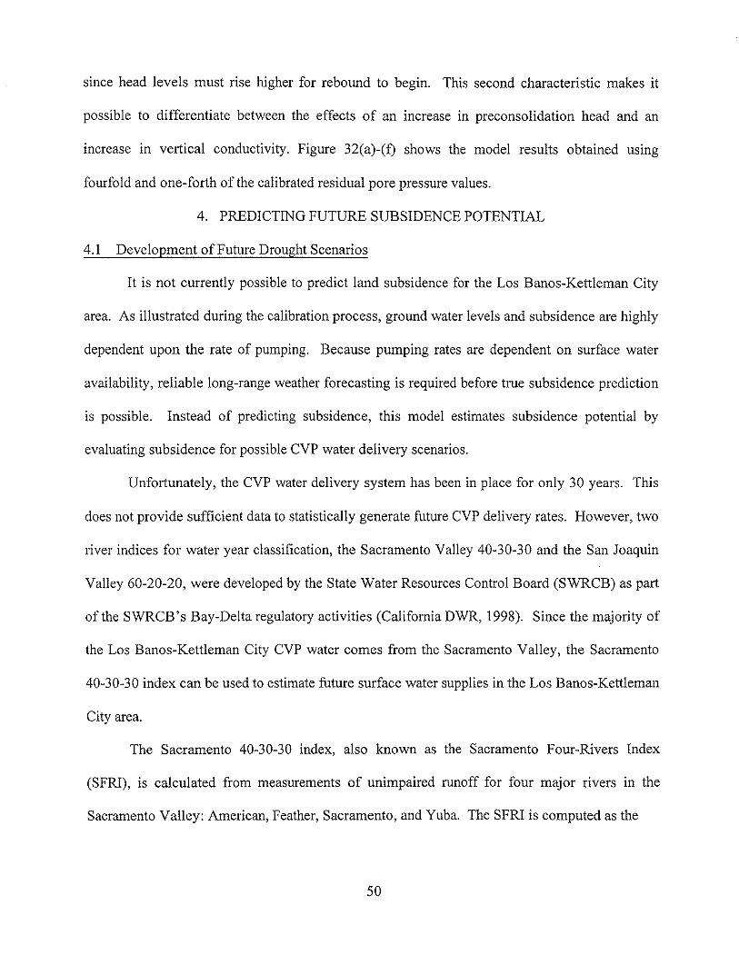
since head levels must rise higher for rebound to begin. This second characteristic makes it
possible to differentiate between the effects of an increase in preconsolidation head and an
increase in vertical conductivity. Figure 32(a)-(f) shows the model results obtained using
fourfold and one-forth of the calibrated residual pore pressure values.
4. PREDICTING FUTURE SUBSIDENCE POTENTIAL
4.1 Development of Future Drought Scenarios
It is not currently possible to predict land subsidence for the Los Banos-Kettleman City
area. As illustrated during the calibration process, ground water levels and subsidence are highly
dependent upon the rate of pumping. Because pumping rates are dependent on surface water
availability, reliable long-range weather forecasting is required before true subsidence prediction
is possible. Instead of predicting subsidence, this model estimates subsidence potential by
evaluating subsidence for possible CVP water delivery scenarios.
Unfortunately, the CVP water delivery system has been in place for only 30 years. This
does not provide sufficient data to statistically generate future CVP delivery rates. However, two
river indices for water year classification, the Sacramento Valley 40-30-30 and the San Joaquin
Valley 60-20-20, were developed by the State Water Resources Control Board (SWRCB) as part
of the SWRCB's Bay-Delta regulatory activities (California DWR, 1998). Since the majority of
the Los Banos-Kettleman City CVP water comes from the Sacramento Valley, the Sacramento
40-30-30 index can be used to estimate future surface water supplies in the Los Banos-Kettleman
City area.
The Sacramento 40-30-30 index, also known as the Sacramento Four-Rivers Index
(SFRI), is calculated from measurements of unimpaired runoff for four major rivers in the
Sacramento Valley: American, Feather, Sacramento, and Yuba. The SFRI is computed as the
50
61 -E~'~'~ I ---~-n-'-"-r---g ",- ----i-- - I I --17 I ~! 'l-, +---1 ' i --~114,5
1.-L_~L ---'r--~i- 1~~i~--l~4LL: I-_~.L~·"J~_~~
.J I I! ! - Observed Subsidence I J3 5 i ~.c__ L 1 -- 125% Pre-consolidetion Head. .r. . i I I -<>-75%Pre-consolidation Head r3 _ ! _~r-_L,-:_~ina~;aHbration I1960 1965 1970 1975 1980 1985 1990 1995 2000
YearA - Extensometer I
€ 'l ~t I j==>,,~ 0-+<0
1
~
~ 3.5 'E·-"-~-r-~~--,-~..--~t;;;! ~~i] 3 ----!---f----.-- J..__ !-_.__ I--:-==+ __
] 2.5·! --~---6 I . !--=:J-.m- ~1
..J 2 .~i __ .1__ -l--~....!..-.J - Observed Subsidence I J
~' Iii! ---125% Pre-consolidation Head ~ 1
1.5 . ~"---f---~ -<>- 75% Pre-consolidation Head f-Ijr.; __ J. ! -1...., i. I-Final :_~Iibr.tio~ ~mmJ i1960 1965 1970 1975 1980 1985
YearC ..Extensometer 3
19951990
3 r--c I "'--1 ---II~ ':r --L-t-:;J -'-"-- --' I, 'llt) I I l~ 1,5 1 __ .. 1· .... ·___ ----1..g IIi I ! j
'" ! ! I i ! i I~ I-I -±±"' ..,.. '''--.. I -s--Observed Subsidence if'1-'
05 j _~~C__ l--~--l ---i25% Pre--cons~lid~tjon Head. I i -<>-75% Pre-consolidation Head
0--- .___ I I _,_2_~- F;na~fa~br.tio:- =! I
1960 1965 1970 1975 1980 1985 1990 1995 2000Year
B - Extensometer 2
7.5 F--II'---'-T I~--"~- I,
7 ' -~----t..----1--------!----L---l-.---:>o:+---i i . I
g 6.5 -~- ...--- - ! r- -;~ ~ l
] 6 -I ---1------- i I r---'" j IJ: 5.5 r---'1- ----I -r"-'-r ! t--l~ 5~! .~~ ,~_~I __ L~r-~:.-Obse~ed sub~id~ce·~~~.J
i ! iii ..•..125% Pre-consolidation Head ! l'
, ii' I 75')'<P I'd' H d i4.5 r---i- '--1-'--1 -o-.;.:,I,J rc-consou anon ca r-" I ~.I Calibration I4 .L.._._~.~_~~ ~ ~ ~=---~-!-"..-, ..-~~t,~!
2000 1985 20001990 19951915 19801960 1965 1970Year
o ..Extensometer 4
Figure 32A-F - Simulated Subsidence for 125, 100 and 75 Percent of Final Calibrated Value ofResidual Pore Pressure at Six Extensometer Locations
51
the sum of 40 percent of the current year's April-July unimpaired runoff, 30 percent of the
October-March unimpaired runoff, and 30 percent of the previous year's SFRl. A cap of 10
MAF is placed on the previous year's index to account for required flood control releases during
wet years (California DWR, 1998).
Figure 33 shows the best fit relationship between the SFRI and the CVP delivery rates for
years classified by the California Department of Water Resources as "below average," "dry," or
"critical." The relationship is mathematically described (R2= 0.7264) as:
(j), = 2 x 10⁻⁷ (SFRI )2.21139
in which CPs is the percent of contracted CVP surface water and SFRI is in million acre-feet.
Historical records of the SFRl are available from 1906 to present. Although this is still
(5)
not enough data to provide any strong conclusion regarding the statistical distribution of the
population, there are enough samples to generate future scenarios using the bootstrap method.
The bootstrap method is based on the assumption that a sample set adequately represents the
entire population and that new scenarios can be generated by sampling with replacement from
the original set. The major restriction of this method is that all sample points must be
independent. Although the SFRl has an obvious one-year lag dependency, the yearly unimpaired
runoff reveals no temporal correlation. Thus, the bootstrap method may be used to generate
unimpaired runoff scenarios. Sampling from the original set using randomly generated uniform
deviates produces potential runoff scenarios. Each thirty-year realization represents an equally
likely runoff scenario for the forecast period, 1999-2028. Each runoff scenario is then
transformed to a SFRI scenario using the 40-30-30 procedure outlined earlier.
The severity of a drought forecast can be measured in several ways. Two such ways
suggested by Shen and Tabios (1996) are average drought severity and cumulative deficit.
52
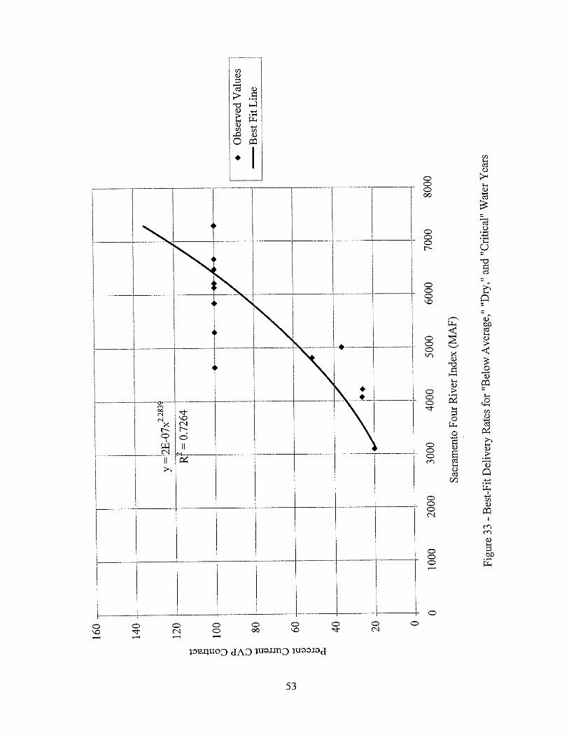
•....
Q Cd
1-< •...
i=:
0 U p.,. > o .....,
i=:
Il) 1-< 1-< :::l
V1
Uw
.....,
i=:
Il) Q 1-< Il) c,
120-+--
I' Ir------~Rr
=O~72
64j
i~---~
~~-~-
·-
100I
I__I.._~__++~-+'/I
!
80I
__~
I__
~~__
..__
.~i
.I
I-
II
t-r-
-_.._-
-~-.-
-.
401-
I!
II
IrI
!
r-1\----------'-1--p---t-------tt
J
\!,'
I
20T~~-.----.---~i..
I··i
o•------l_.~l_-_=~r--T~--I----i-------·-+l
!------.-~--!.--
....--j--..-L-l~--.-..J
o10
0020
0030
0040
0050
0060
0070
0080
00
Sacr
amen
toFou
rRiv
erIn
dex(
MA
F)
Fig
ure3
3-B
est-FitD
eliv
eryR
ates
for"B
elow
Ave
rage
,""Dry,"
and"Critical"
Wat
erY
ears
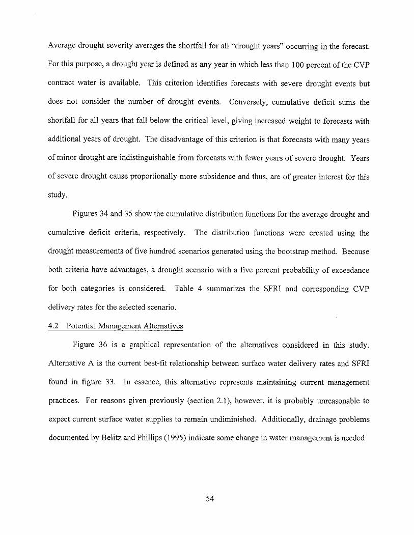
Average drought severity averages the shortfall for all "drought years" occurring in the forecast.
For this purpose, a drought year is defined as any year in which less than 100 percent of the CVP
contract water is available. This criterion identifies forecasts with severe drought events but
does not consider the number of drought events. Conversely, cumulative deficit sums the
shortfall for all years that fall below the critical level, giving increased weight to forecasts with
additional years of drought. The disadvantage of this criterion is that forecasts with many years
of minor drought are indistinguishable from forecasts with fewer years of severe drought. Years
of severe drought cause proportionally more subsidence and thus, are of greater interest for this
study.
Figures 34 and 35 show the cumulative distribution functions for the average drought and
cumulative deficit criteria, respectively. The distribution functions were created using the
drought measurements of five hundred scenarios generated using the bootstrap method. Because
both criteria have advantages, a drought scenario with a five percent probability of exceedance
for both categories is considered. Table 4 summarizes the SFRI and corresponding CVP
delivery rates for the selected scenario.
4.2 Potential Management Alternatives
Figure 36 is a graphical representation of the alternatives considered in this study.
Alternative A is the current best-fit relationship between surface water delivery rates and SFRI
found in figure 33. In essence, this alternative represents maintaining current management
practices. For reasons given previously (section 2.1), however, it is probably unreasonable to
expect current surface water supplies to remain undiminished. Additionally, drainage problems
documented by Belitz and Phillips (1995) indicate some change in water management is needed
54
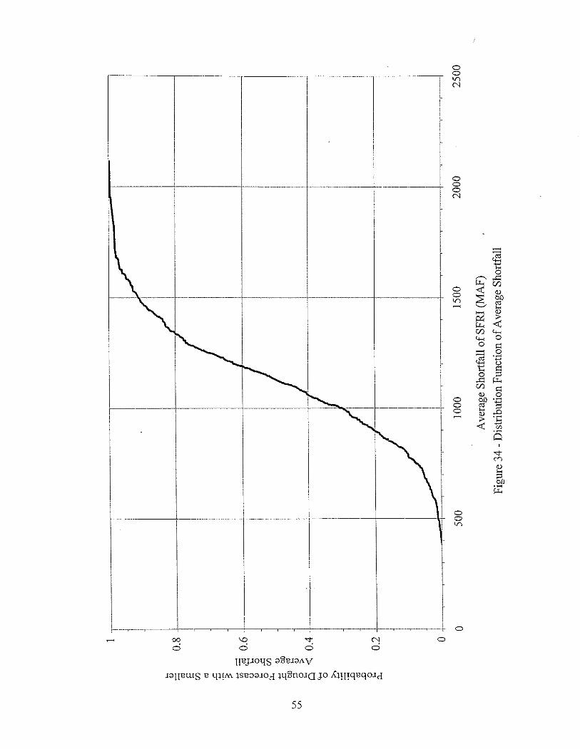
I!-
I-I-~g! f ~
II
t1---L--~- t ~
Ii --+-~, I 0I~ !~
•.....• 00 \0 "<:t 0J 00 0 0 0
~--.
I
I
I1BJ.IOqS g13B.IgAV.IgIlBWS B ql!M lS13;)g.IOdlqZlnOJG JO Al!I!qBqOJd
55
ooI.()
N
oooN
ooI.().-
.-~t::0,.--.., ,...c:
~ 1ZJ-< v~ OJ)ro<;» •....;;Z v;>~ <r::r/.l 4--14-< 00 ~- 0~
, .-<+-'Ut:: ~
0 :::l,...c: ~o: ~v 0OJ) '§~v :-9;> .t:J-< (/),-0<::tM
V•....:::lOJ)i:.I:
V1 0'1
H ~ ~ E if] «j {3 .~..-
•.-<
o()
·c~
«j
Q)5
Q()
Q)if]
.:::..-•...
..c
«j
0.0-
;:l;:l
o6
H;:l
QU
4-< o 4q - ~ ..D o H p..
1r----~~r-~----
r---------~-l----------'-
---
I---l
iI!
I!
~J
0_8r---~I---"-~~I'"
-~~
----.1
~.-.····----r---~----~l
~,
II
iI
IJ
06t--~-·1----·----
_...--------u-l----..-····----·-~1
oJ
I-T'.-------------~.--.-
...---.---J~
+-_.._....----'
II
'I
\
Ii
;I
II
II
0.2I
I?~~I-·
.----,--
! -1 I .\ I ..~
o
r-"--
i
5000
1000
015
000
-'·~~-·1~
-.-,
..--r-~
._r-~~
1---
;I
i
2000
030
000
3500
025
000
Cum
ulativeDeficitof
SFRI(M
AF)
Figure
35-Distribution
Functionof
Cum
ulativeDeficit
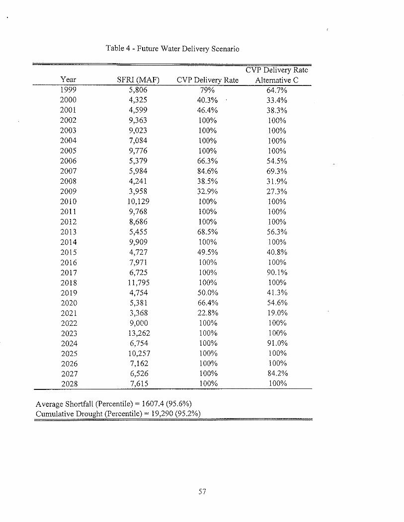
Table 4 - Future Water Delivery Scenario
Year SFRI (MAF) CVP Delivery RateCVP Delivery RateAlternative C
199920002001200220032004200520062007200820092010201120122013201420152016201720182019202020212022202320242025202620272028
5,8064,3254,5999,3639,0237,OS49,7765,3795,9844,2413,95810,1299,7688,6865,4559,9094,7277,9716,72511,7954,7545,3813,3689,00013,2626,75410,2577,1626,5267,615
79%40.3%46.4%100%100%100%100%66.3%84.6%38.5%32.9%100%100%100%68.5%100%49.5%100%100%100%50.0%66.4%22.8%100%100%100%100%100%100%100%
64.7%33.4%38.3%100%100%100%100%54.5%69.3%31.9%27.3%100%100%100%56.3%100%40.8%100%90.1%100%41.3%54.6%19.0%100%100%91.0%100%100%84.2%100%
Average Shortfall (Percentile) = 1607.4 (95.6%)Cumulative Drought (Percentile) = 19,290 (95.2%)
57
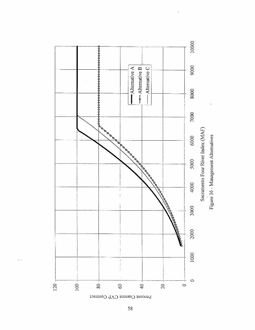
•.. () ro l-< •....
C 0 U 0... > U C ([) l-< l-<
V1
;:l00
U ...., c ([) o l-< Q) 0
...
120-,-
II
I I I100·1··~ I I
80.f-!--
60·
..
20+--..---
--1
o+-
-~~1
I
.~··l·--·····---
·-I
o
Ii--
I
4000
-AlternativeA
40r--
II
I-i-7'75>1
Ii1-0-
AlternativeB
I
II
IY~
II
-AlternativeC
I l----tl-----+I
----+I
-~-_+_I
---I
.J~
II
I
1000
2000
3000
5000
6000
7000
8000
9000
10000
Sacram
ento
Four
River
Index(M
AF)
Figure
36-M
anagem
entAlternatives
for agriculture to remain viable in the Los Banos-Kettleman City region. Two additional
alternatives addressing these issues are also considered.
As one possible solution to the drainage problems in the region, Belitz and Phillips
(1995) proposed a combination of increased ground water pumpage and reduced recharge. Their
proposal is considered as alternative B and is summarized by the water budget given in Table 5.
It is an attractive alternative because it would reduce many of the drainage problems in the
region. It would also require only minimal investment, as all increases in pumping would occur
at existing wells. It is assumed that the relationship between percent CVP delivery rates and
SFRI remains the same as in Alternative A, but that the 100 percent delivery rate is reduced to
the rate proposed by Belitz and Phillips (1995).
Alternative C reduces surface water demand not by changing the total contracted amount
of surface water, but by changing the relationship between percent delivery rate and SFRl. By
increasing the SFRl required to result in a 100 percent CVP delivery rate, Alternative C reduces
the surface water used during drought years. During wet years there is no reduction in total
surface water use. During drier years, however, surface water use is reduced up to 20 percent for
years of moderate drought, with more modest reductions during years of severe drought. (see
figure 36) Although this alternative would provide a reduction of up to 153,000 acre-feet of
surface water during years of drought, it does little to address the drainage and water quality
problems facing the region.
4.3 Optimization Model
A linear optimization model was formulated to find the maximum increase in ground
water withdrawal without causing any inelastic compaction during the 30-year planning horizon.
In order to eliminate the nonlinearity associated with subsidence, heads are allowed to fluctuate
59
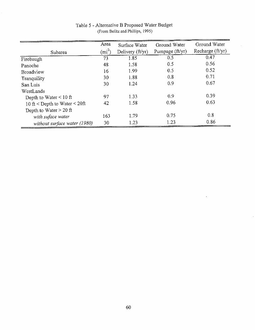
Table 5 - Alternative B Proposed Water Budget(From Belitz and Phillips, 1995)
Area Surface Water Ground Water Ground Water
Subarea (mi'') Delivery (ftlyr) Pumpage (ft/yr) Recharge (ft/yr)
Firebaugh 73 1.85 0.5 0.47
Panoche 48 1.58 0.5 0.56
Broadview 16 1.99 0.5 0.52
Tranquility 30 1.88 0.8 0.71
San Luis 30 1.24 0.9 0.67
WestLandsDepth to Water < 10ft 97 1.33 0.9 0.39
10 ft < Depth to Water < 20ft 42 1.58 0.96 0.63
Depth to Water> 20 ftwith suface water 163 1.79 0.75 0.8
without surface water (1980) 30 1.23 1.23 0.86
60
only within the region of elastic compaction. This is accomplished by setting the
preconsolidation head as the lower bound for ground water levels in the confined aquifer. For
simplicity in computation and implementation, the optimization model assumes uniform
pumping over each pumping subarea and heads are only monitored at one characteristic location
in each subarea.
A response function approach (Gorelick, 1983; Yeh, 1992) is used in the model
formulation. In this approach, the calibrated simulation model is used to generate response
coefficients. The model is first allowed to reach a steady state under normal-year pumping
conditions. Each pumping subarea is then separately subjected to a unit impulse of additional
pumpage in the first period with no disturbance thereafter, and the system response to each
excitation is monitored over the entire planning period. All the responses are then assembled in
a response matrix. This response matrix can subsequently be used in the formulation of the
following optimization model.
The objective function of the optimization model maxinuzes the total ground water
withdrawal at all production wells during the forecast period:
NI'S NOW
Max z:;:, I IQ(k,n)It=! k~J
(6)
in which Z is the value of the objective function (L); Q(k,n) is volume of water withdrawn from
the klh well field (L3/T); NTS is the total number of periods; NOW is the total number of well
fields; and n is the time index.
The constraint set of the model includes the following conditions and specifications:
61
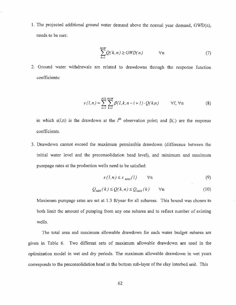
1. The projected additional ground water demand above the normal year demand, GWD(n),
needs to be met:
NOW
LQ(k,n);;:: GWD(n)k~J
\:in (7)
2. Ground water withdrawals are related to drawdowns through the response function
coeffi cients:
NTS NOW
s(l,n)-;::; L "Lf3(l,k,n-i+l)'Q(kfl)n«! k~J
'Ill, 'lin (8)
in which s(l,n) is the drawdown at the lh observation point; and ~(.) are the response
coefficients.
3. Drawdown cannot exceed the maximum permissible drawdown (difference between the
initial water level and the preconsolidation head level), and minimum and maximum
pumpage rates at the production wells need to be satisfied:
s(l,n) ~s MAX(l) Vn (9)
\in (10)
Maximum pump age rates are set at 1.3 ft/year for all subareas. This bound was chosen to
both limit the amount of pumping from anyone subarea and to reflect number of existing
wells.
The total area and maximum allowable drawdown for each water budget subarea are
given in Table 6. Two different sets of maximum allowable drawdown are used in the
optimization model in wet and dry periods. The maximum allowable drawdown in wet years
corresponds to the preconsolidation head in the bottom sub-layer of the clay interbed unit. This
62
Table 6 - Maximum Drawdowns and Areas for Pumping Subareas
1 6 8Water Budget Subareas9 10 lla 11b lIe lId
Smax-dry (feet)Smax-wet (feet)
Area (mi")
141.6
95.9
73
124.883.4
30
152.897.5
48
172.5 225.2 153.1109.6 175.8 98.8
16 30 98
168.4105.4
41
195.3116.9
148
269.7214.2
45
63
is the maximum preconsolidation head for any compressible layer. Because of the low
conductivity of the clay layer, however, piezometric head levels in the confined aquifer may drop
below this value for short periods without causing inelastic subsidence. To take advantage of
this additional capacity, the maximum allowable drawdown during dry years corresponds to the
preconsolidation head in the outermost layer of the clay interbed unit. This adjustment provides
for additional drawdown during periods of drought, but sustains long-term head levels above all
values of preconsolidation head.
The calibrated MODFLOW (McDonald and Harbough, 1992) model was used to derive
the response coefficients. The optimization model formulated above is a linear programming
model and was solved using GAMS (Brook et al., 1992). The pumping rates calculated by the
optimization model were then returned to the simulation model to estimate land subsidence.
4.4 Results
Figures 37-42 present the model predictions of total subsidence for the years 1999 to
2028 at the six extensometer locations used for calibration. Contour maps of land subsidence
across the entire study area are shown as Figures 43-45.
Alternative A causes very little subsidence. Although there is some elastic compaction
during years of drought, the overall trend is toward rebound. Alternative B causes significant
subsidence, especially in the northwest corner of the model. At extensometers 13112-20D 1,
15/13-11D2, and 161l5-34Nl, subsidence occurs predominantly during periods of drought. At
the other extensometer locations, subsidence continues during normal water years as well.
Alternative C produces subsidence similar to that of alternative A. In general, the compaction is
elastic and long-term subsidence is minimal. A small increase in inelastic compaction during
periods of drought accounts for the difference between the two alternatives. The optimization
64
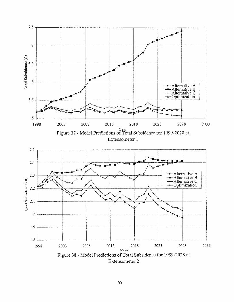
7.5 ~-~~~~r,'~"'-""""-'-"--"-r'---' III
7 -+--------I-----Li . Ig ! I
j 6.5 +--1 --·--+-----1 --. '---1 -..- ~
~ 6 •. I ! ~I - -----~j I II I -- Alternative A I ii I -II- Alternative B ! III--+- Alternative C I I:
! l --6-- Optimization5.5 -·---~""""';'------·i---·---·-----·---- .---.-._-- ....---------- --.~=~- --=~~.~.___l
I I
II !I. !I I5 .1.-----I-------·--+__1 -----1-----------+-------- ---J-------j
1998 2003 2008 2013 2018 2023 2028 2033Year
Figure 37 - Model Predictions of Total Subsidence for 1999-2028 atExtensometer 1
2.5 r- -----..-1 ---,.-1---···-·---- -·---~-----r------i2.4\-~--+--~----J--.....~=-==i~~--+---- __i .._. ._...._1
'! '_1_ -II:::~I:~~:ll~~~-I-l~ , I n ~ Alternative C ,r2 L----I------·-----i "y --1----- II ":".~ 21 I i -~ I =i~--.-.--~2-1~-+--1 I I -~
:::r+ L I --C-- L-..---l---j1998 2003 2008 2013 2018 2023 2028 2033
YearFigure 38 - Model Predictions of Total Subsidence for 1999-2028 at
Extensometer 2
65
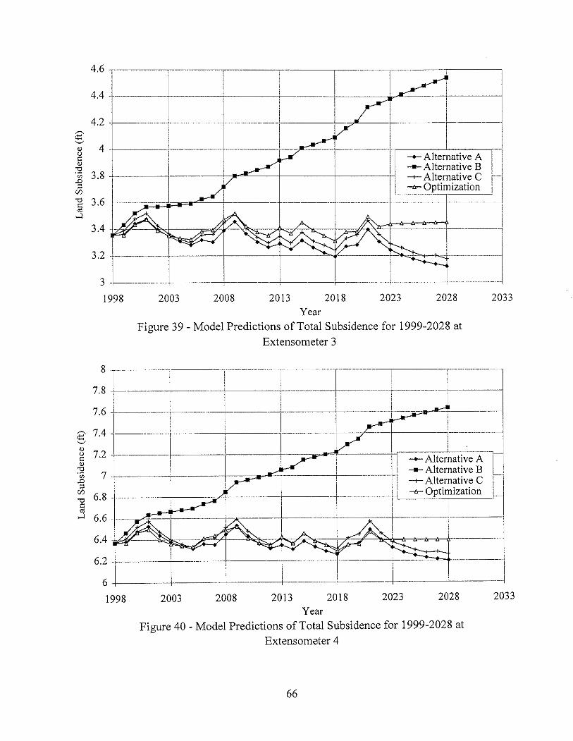
~ 4.:' ---=- ' ---I ! .~ I ~ -I~ --1--- -----!I ~-·-----I·,-----A-lt-e...lrn-a-ti-ve-A--r-l
:g I -- Alternative B I
.2 3.8 I 'l -+- Alternative C i·j~ .__..~ Slp!}mization _J I'"8 3.6 .----.=:a::iF-pIt'=--t---- .---+--~-~t--------1
j 3.4 [ -'r-l:t---Q-_-i:r_~~··_-¢.I--·--~
I '!""l~~.4/ I i, : 1
3.2 J ~-.--.----+---~~ L j3 -L--~----l ! - ~~~c=--1998 2003 2008 2013 2018 2023 2028 2033
YearFigure 39 - Model Predictions of Total Subsidence for 1999-2028 at
Extensometer 3
8 r--·-··~·i I 1- ]--------1 r------17.8 -I ----+---.-t ,-- 1--------------1--·----··--- -1-~--·-1
»<. 7.6 t----·--·t--j--r i T=_ ~r------··--I~::L---.~J 1 --1"--- .- -!-----------: r--- -T---~-~~-,J~ I iii Iii -- Alternative A I I~ 7 T 1i
------~ ~----- : . ··--··-M =:~~~~~~:~~~~g l::: 6.8 J_ __ _ i -- ...--L-J..------I i -fr- Optimization LI
~ I I ~I I I r --"l ~6.6 -!-~ --.-L I -~~l T---r-·--~-6.4 J ...' .--------\6.2 +---.+=-- '-··_-'-16L--...._-l--- 1 ._-_.--i
1998 2003 2008 2013 2018 2023 2028 2033Year
Figure 40 - Model Predictions of Total Subsidence for 1999-2028 atExtensometer 4
66
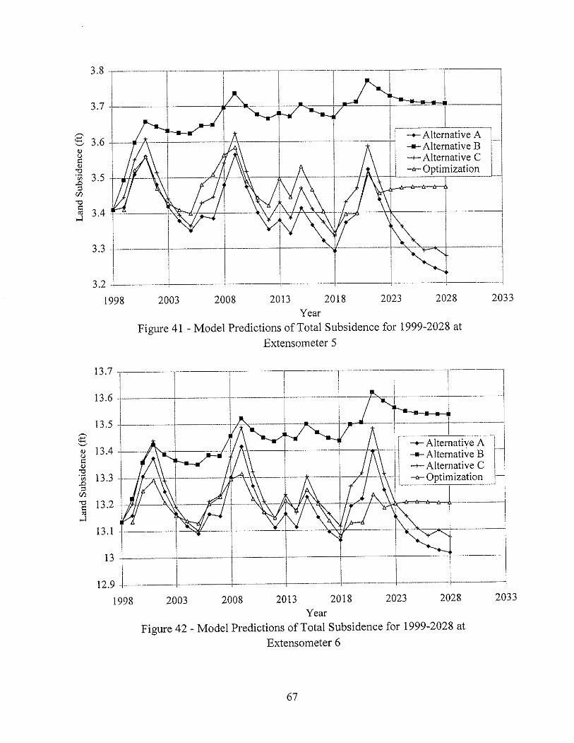
~---f-···-~~-f-----
\+-------~ _ __!_ __ -1
~~---~I .i !
J~-~-;---.~J1998 2003 2008 2013 2018 2023 2028 2033
YearFigure 41 - Model Predictions of Total Subsidence for 1999-2028 at
Extensometer 5
·--··-ir----~--~~~·
I--1
I-.--i--.-.~~
I-L---J2003 2008 2013 2018 2023 2028 2033
YearFigure 42 - Model Predictions of Total Subsidence for 1999-2028 at
Extensometer 6
67
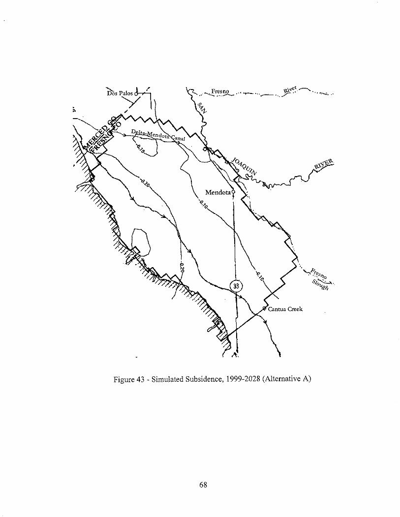
F '<.let ----..-...,_resng ,'. __ ... ~... ' .. ~.• ---....._,~ ,..,.- .~~..,/ . I'
Figure 43 - Simulated Subsidence, 1999-2028 (Alternative A)
68
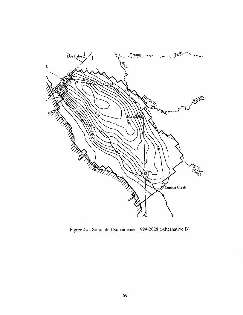
''let, ...-,.,., •....., Fresno .'" ""i""'- '" ~ ." ' •• --.:.. '.' ---.... .... ~ ,....---.,./ . .
Figure 44 - Simulated Subsidence, 1999-2028 (Alternative B)
69
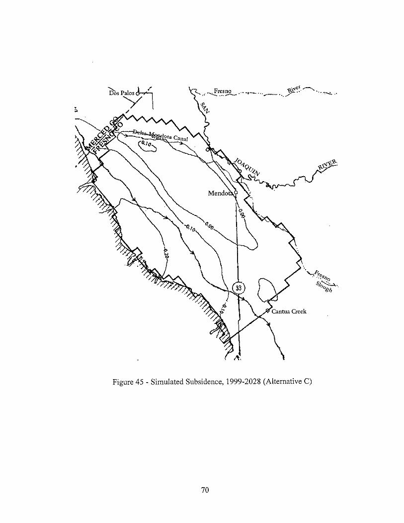
Figure 45 - Simulated Subsidence; 1999-2028 (Alternative C)
70
results produce subsidence similar to that of Alternatives A and C. The only major difference is
a period of little change during the final seven years while Alternatives A and C show significant
rebound.
The maximum ground water withdrawal for each water budget subarea found in the
optimization model is shown in Fig. 46. Ground water withdrawal can be significantly increased
without causing any inelastic compaction in subareas 1 (Firebaugh) and 6 (Tranquillity). These
subareas are located along the river in the eastern side of the basin. In contrast, withdrawals
cannot be increased above the minimum required rate over the next two decades without leading
to inelastic subsidence in subareas 10 and 11 along the no-flow boundary to the west. Ground
water supplies are intensely operated in almost all of the subareas during the last years of the
future scenario. This is the result of one of the major assumptions of the optimization model.
Since the optimization model has perfect foresight, following the final drought period it must no
longer plan for future drought and can increase pumping until ground water levels reach the
point of maximum drawdown. In general, from the standpoint of land subsidence, there is
greater potential for increased withdrawal of ground water supplies on the eastern side of the
basin than on the western side.
5. CONCLUSIONS AND RECOMMENDATIONS
For the foreseeable future, land subsidence will remain a concern for water managers in
the San Joaquin Valley. To avoid the costly and serious damage associated with land
subsidence, it is vital to consider the effects of all proposed water use alternatives. The ground
water-subsidence model presented herein provides a method for evaluating each alternative.
The success of a model is mainly measured by its ability to reproduce observed data.
Although it cannot represent the complex ground water system in its entirety, the Los Banos-
71
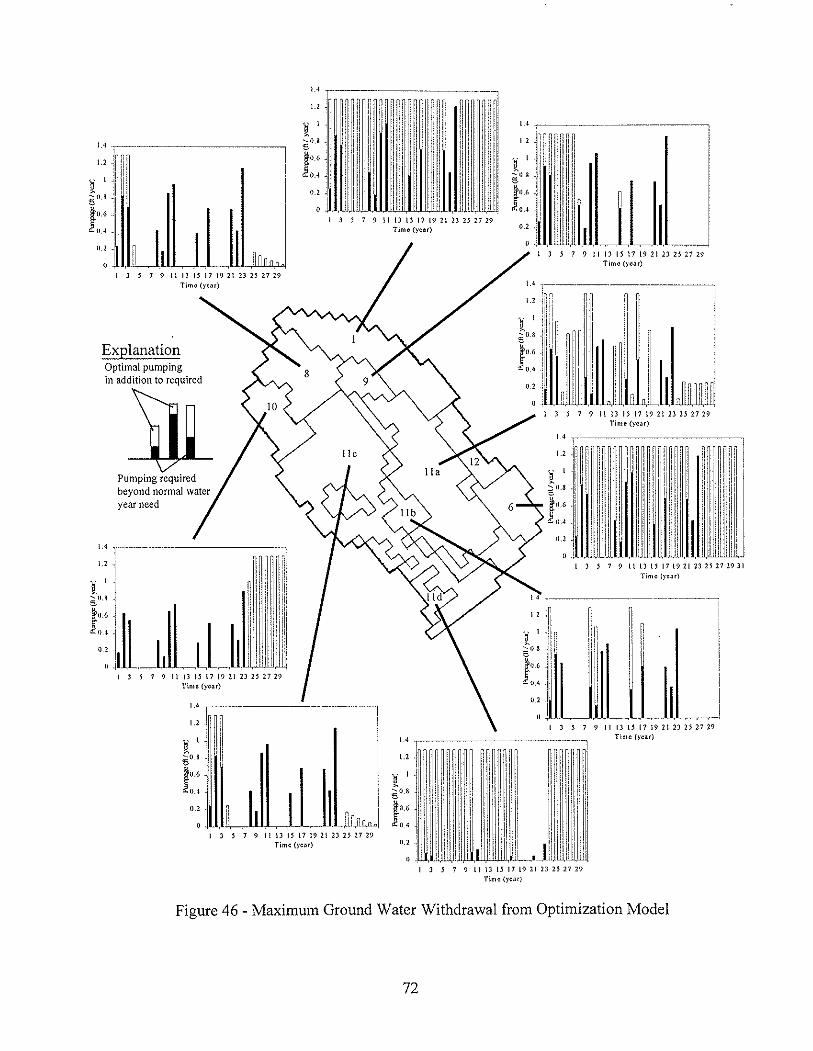
U --.--~ ... . ,
l.l ~ 111 il![ DI!i ~r~i~j 111!lr r,~I rll'i~1'~' I I II, Ii' iii I III' IIII IIII1 IIII1
~ ~O.i '1'1'11 Iii II 1 ill I I i :I~illl! t: III IIII'! III 11,11111'11
0.2 I II" ., III ~. I II Iii III i ,Ii i I IiII ,II! T I I • , ,j •._,1 L~
-' I I J 5 7 9 II 13 15 11 19 21 23 25 27 29
ITime {year)
.-~,,~
-~W_W--~--"lII
I 3 5 7 9 I I D 15 17 19 21 23 25 27 29Time (year)
ExplanationOptimal pumpingin addition to required
ui~~----nll-'-n~----:Uj,i!ii li!1 i,
'"I III' ,h lilli', I' i ;'::-0,8 i,ll, 1'1 III ~ I IIS sun I
JO'.6 ",:,i"1 ~ I I, ] Ii I i'I ' I' i i•..• U 4 j 1 ~ l 1
0.2 '.:,JI nil] !III~illt,~'1lrloJ," 1." L[ . J I IIII 3 5 7 9 II IJ Il 17 19 21 2J 25 27 29
Time (YCH)
Pumping requiredbeyond normal wateryear need
I J l 7 9 11 IJ 15 I 7 19 21 23 25 27 29Time (year)
,::mf£'03 .1 I'!I
J:': l0.2 ~
O. ,",~.LI 3 s 7 9 111315171921232527 29
Time (year)
-----'---1Ii
I 3 5 7 9 II 13 IS 11 19 21 2 J 2S 27 29Tjm c (>'-c:.u)
Figure 46 - Maximum Ground Water Withdrawal from Optimization Model
72
Kettleman City model is a simplified conceptual model that successfully matches observed head
and subsidence values. Because of the limited amount of data available and the corresponding
large number of calibration variables, however, it is possible that other model parameters could
produce equally appropriate matches to the observed data. Although the model is probably not
unique, the current calibrated model appears to be sufficient for the evaluation of future water
management alternatives.
If present practices can be sustained for the Los Banos-Kettleman City area, land
subsidence will not be a serious problem in the next thirty years. Although head levels are
significantly reduced and some elastic compaction does occur during periods of drought, there is
enough storage in the underlying aquifers to prevent most non-recoverable subsidence.
However, with the continued growth of urban populations to the south and concerns over the
ecological implications of water exportation from the north, there seems to be little hope of
sustaining current practices.
The alternative water budget proposed by Belitz and Phillips (1995) achieves a reduction
in surface water dependency by increasing irrigation efficiency and ground water pumping. This
proposal is also meritorious for its positive effect on drainage problems in the region.
Unfortunately, this alternative produces significant inelastic subsidence during the future
scenario considered in this report.
There are two possible reasons the Belitz and Phillips report (1995) did not recognize the
proposed water budget's potential for subsidence. First, in their analysis, subsidence was
assumed to occur only when the piezometric head in the confined aquifer falls below its past
minimum. This neglects the presence of residual pore pressure, which will cause inelastic
compaction to begin at heads much greater than the past aquifer minimum. Second, in the water
73
budget used by Belitz and Phillips (1995), the surface water delivery rate was assumed to be
constant for the next 45 years. Much of the predicted subsidence would be eliminated using the
same assumption for our model. The proposed water budget lowers head values just enough,
however, that when drought years are included, there is not enough storage to prevent subsidence
from occurring.
The final alternative examined was a shift in the relationship between available surface
water (SFRI) and the amount of CVP water used in the region. Like Alternative A, this
alternative limits subsidence to an acceptable rate. Although it does not reduce the surface water
required during wet years, it reduces the area's dependence on surface water during years of
drought. This or any other alternative that involves an increase in pumping is potentially limited
by water quality problems (e.g., TDS, salinity). Although the modest increases in pumpage
included here are probably acceptable (Belitz and Phillips, 1995), additional work would be
required to determine the long-term impact of such changes on water quality.
A linear optimization model was constructed to predict the maximum potential ground
water pumpage from each subarea above the predicted water demands for the next 30 years.
Although perfect foresight limits the implementation of the optimization model in practice, the
model indicates that ground water supplies of certain subareas in the eastern portion of the study
area can be operated far above the target demand rates without leading to inelastic compaction.
In contrast, little increase in ground water withdrawal is possible for subareas on the western
side.
There are at least three areas in which further work could improve the quality of the
model. First, the thickness of the layer representing the interbeds was assumed to be uniform
across the study area. Additional field data regarding the composition of the confined aquifer
74
may allow for a better estimation of the spatial distribution of interbed thickness. Second, the
model only considers yearly stress periods. Some detail is lost as pumping is averaged over the
entire year. A seasonal or monthly model may capture more accurately the ground water
fluctuations leading to subsidence. Finally) the time delay of compaction was adequately
captured using the IBS 1 package (Leake) 1991) by sub-dividing the compressible layers.
However) equally valid and numerically more efficient results may also be attainable using a
package which analytically considers time delay, such as the IDP package (Shearer and Kitching,
1994).
75
REFERENCES
American Farmland Trust. 1995. Alternatives for Future Urban Growth in California's CentralValley: The Bottom Linefor Agriculture and Taxpayers. Washington, D. C., U.S.A.
Belitz, K., and Heimes, F.J. 1990. Character and evolution of the ground water flow system inthe central part of the western San Joaquin Valley, California. U.S. Geological SurveyWater-Supply Paper 2348: 28p.
Belitz, Kenneth, Phillips, S. P., and Gronberg, J. M. 1992. Numerical Simulation of Ground-Water Flow in the Central Part of the Western San Joaquin Valley, California. U. S.Geological Survey Open-File Report 91-535: 71 p.
Belitz, Kenneth and Phillips, Steven P. 1995. Alternatives to Agricultural Drains in California'sSan Joaquin Valley: Results of a Regional-Scale Hydrogeologic Approach. U. S. GeologicalSurvey Open-File Report 91-535: 71 p.
Brooke, A., Kendrick, D., and Meeraus, A. 1992. Release 2.25 GAMS (General AlgebraicModeling System) A User's Guide. Boyd & Fraser Publishing Company, Danvers,Massachusetts, p. 289.
Bull, W. B., and Miller, R. E. 1975. Land subsidence due to ground water withdrawal in the Los-Banos Kettleman City area, California. Part 1, Changes in the hydrologic environmentconducive to subsidence. U.S. Geological Survey Professional Paper 437-E: 7lp.
Bumb, A. C., Mitchell, 1. I., and Gifford, S. K. 1997. Design of a ground-water extraction/re-injection system at a superfund site using MODFLOW. Ground Water 35(3):400-408.
California Department of Water Resources. 1998. Compaction Recorded by Extensometer-WellsSince 1984 in the West San Joaquin Valley, California. Sacramento, California.
California Department of Water Resources. 1999. California Water Plan Update, Bulletin 160-98, v. 1
Casagrande, A. 1932. The Structure of Clay and its Importance in Foundation Engineering,Journal of the Boston Society of Civil Engineers, April; reprinted in Contributions to SoilMechanics 1925-1940, BSCE:72-113
Gorelick, S. M. 1983. A review of distributed parameter ground-water management modelingmethods. Water Resources Research. v, 19, no. 2, pp. 305-319.
Gronberg, J. M. and Belitz, Kenneth. 1992. Estimation of a Water Budget for for the CentralPart of the Western San Joaquin Valley, California. U. S. Geological Survey Water-Resources Investigation Report 91-4192: 22 p.
76
Holtz, Robert D. and Kovacs, William D. 1981. An Introduction to Geotechnical Engineering.Prentice Hall, Englewood Cliffs, New Jersey: 733 p.
Holzer, T. L. 1989. State and Local Response to Damaging Land Subsidence in United StatesUrban Areas. Engineering Geology 27:449-466.
Hua, Z., Tiezhu, L., and Xinhong, L. 1993. Economic benefit risk assessment of land subsidencein Shanhai. Environmental Geology 21 :208-211.
Hubbell, 1. M., Bishop, C. W., Johnson, G. S., and Lucas, 1. G. 1997. Numerical ground-waterflow modeling of Snake river plain aquifer using superpostion technique. Ground Water35(1):59-66.
Ireland, R. L., Poland, 1. F. and Riley, F. S. 1984. Land Subsidence in the San Joaquin Valley,California, as of 1980. U. S. Geological Survey Professional Paper 437-1: 93p.
Ireland, R. L. 1986. Land subsidence in the San Joaquin Valley, California, as of 1983. Preparedin cooperation with the California Department of Water Resources, Sacramento, California.U.S. Geological Survey, Denver, CO: 50 p.
Johnson, A. I., Moston, R. P., and Dorris, D. A. 1968. Physical and hydrologic properties ofwater-bearing materials in subsiding areas in the central California. U.S. Geological SurveyProfessional Paper 497-A: 71p.
Laudon, J., and Belitz, K. 1991. Texture and depositional history of Late Pleistocene-Holocenealluvium in the central part of the western San Joaquin Valley, California. Bulletin of theAssociation of Engineering Geologist 28(1):73-88.
Leake, S. A. 1990. Interbed storage changes and compaction in models of regional ground waterflow. Water Resources Research 26: 1939-1950.
Leake, S. A., and Prudic, D. E. 1991. Documentation of a computer program to simulate aquifer-system compaction using the modular finite-difference ground water flow model. U.S.Geological Survey Techniques of Water Resources Investigation, Book 6, Chapter A2: 68 p.
Leake, S. A. 1991. Simulation of vertical compaction in models of regional ground-water flow.pp. 565-574. In: Proceedings of the fourth international symposium on land subsidence, May1991. lARS Publication no. 200.
Lofgren, B. E. 1979. Changes in Aquifer-system Properties with Ground Water Depletion. pp.26-46. In: Procedings, International Conference on Evaluation and Prediction of LandSubsidence, Pensacola, December 1978. American Society of Civil Engineers.
McDonald, M. G., and Harbaugh, A. W. 1988. A modular three-dimensional finite-differenceground-water flow model. U. S. Geological Survey Techniques of Water ResourcesInvestigations, Book 6, Chapter AI: 586 p.
77
Miller, R. E., Green, J. E., and Davis, G. H. 1971. Geology of the compacting deposits in the LosBanos-Kettleman City Area, California. U.S. Geological Survey Professional Paper 497-E:46p.
Onta, P. R., and Gupta, A. D. 1995. Regional management modeling of a complex ground watersystem for land subsidence control. Water Resources Management 9:1-25.
Page, R. W. 1986. Geology of the fresh ground water basin of the Central Valley, California,with texture maps and sections. U.S. Geological Survey Professional Paper 1401-C: 54p.
Phillips, Steven P. and Belitz, Kenneth. 1991. Calibration of a Texture-Based Model of aGround-Water Flow System, Western San Joaquin Valley, California. Ground Water29(5):702-715
Poland, J.F., Lofgren, B.E., Ireland, R.L., and Pugh, R.G. 1975. Land Subsidence in the SanJoaquin Valley, California, as of 1972. U.S.G.S. Professional Paper #437-H. U.S.Government Printing Office, Washington D.C., U.S.A.
Poland, J. F. 1981. The Occurrence and Control of Land Subsidence Due to Ground-WaterWithdrawal with Special Reference to the San Joaquin and Santa Clara Valleys, California.Ph.D.-Dissertation, Stanford University, Palo Alto, California
Reynolds, J. W., and Spruill, R. K. 1995. Ground-water simulation for management of aregulated aquifer system: A Case study in the North Carolina Coastal Plain. Ground Water33(5):741-758.
Shearer, T. R., and Kitching, R. 1994. A numerical model of land subsidence caused by groundwater abstraction at Hangu in the peoples of republic of China. British Geological Survey,Technical report WC/94/46
Shearer, T. R. 1998. A numerical model to calculate land subsidence, applied at Hangu in China.Engineering Geology 49:85-93.
Shen, H. W. and Tabios, G. Q. 1996. Modeling of Precipitation-Based Drought CharacteristicsOver California. Technical Completion Report. Water Resources Center, Contribution No.204. Water Resources Center. University of California, Davis
Sophoc1euos, M., and Perkins, S. P. 1993. Calibrated models as management tolls for stream-aquifer systems: the case of central Kansas, USA. Journal of Hydrology 152:31-56.
Terzaghi, K. 1925. Principles of soil mechanics: IV Settlement and consolidation of clay. In:Eng. News-Rec, McGraw-Hill, New York:874-878.
Williamson, A. K., Prudic, D. E., and Swain, L. A. 1989. Ground water flow in the CentralValley, California. U.S. Geological Survey Professional Paper 1401-D: 127 p.
78
Wilson, A. M., and Gorelick, S. 1996. The effects of pulsed pumping on land subsidence in theSanta Clara Valley, California. Journal of Hydrology 174:375-396.
Yeh, W-G. W. 1992. System analysis in ground-water planning and management. Journal ofWater Resources Planning and Management, ASCE. v. 118, no: 3, pp. 224-237.
79
APPENDIX
80
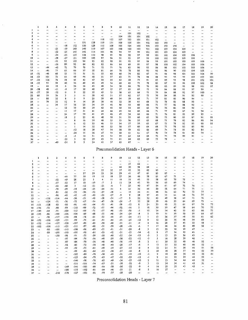
81
82
83
10 II 12 13 14 15 16 17 18 19 20I2 39 433 25 33 40 444 ·4 5 16 28 35 42 445 ·41 -n ·15 -2 7 24 31 41 43 466 -65 ·61 .45 ·37 ·22 ·9 4 18 29 39 41 45 497 -75 ·69 ·63 ·53 ·46 .}2 ·15 ·4 IS 28 35 39 44 48 533 ·80 -75 ·68 ·63 -59 ·41 ·22 ·10 12 24 J2 36 42 46 529 ·87 .84 -19 -80 -67 ·55 ·31 ·13 8 21 28 J2 40 45 51 54
!G -100 ·95 -95 -86 ·71 ·59 ·38 ·18 3 16 24 29 37 43 49 5311 -110 ·108 -104 -96 -77 -62 ·45 ·22 .3 II 19 27 35 42 48 52 5612 ·126 ·122 -114 .99 ·83 ·66 ·52 -29 -9 7 15 24 32 40 47 51 5613 -157 -146 -136 ·122 ·102 ·87 ·68 ·56 .}4 ·16 2 11 21 29 38 46 50 5514 ·162 -155 ·147 -131 ·112 -88 -n ·59 ·41 .21 ·4 1 16 27 36 43 49 5415 ·185 ·169 ·162 ·157 ·144 ·120 ·94 -76 ·61 .45 ·27 ·10 a 14 24 34 41 47 53 5816 -192 ·178 ·172 -168 -159 -134 -96 -78 ·64 ·50 ·32 ·16 ·2 10 22 30 39 46 52 5817 -194 ·185 -176 -168 -159 -129 ·94 -80 ·66 -52 ·37 ·21 ·1 7 18 26 35 43 49 5718 -196 .190 .171 ·161 ·150 -120 ·92 ·80 ·67 -55 -42 ·27 ·12 3 14 23 33 42 48 5J19 -190 -178 ·165 ·141 ·1l0 ·89 .79 ·67 -58 .45 ·30 ·16 ·3 11 21 3 I 39 45 4820 -206 -190 ·178 ·165 ·141 ·113 ·90 ·78 -70 .62 .48 ·31 ·17 ·3 II 21 29 38 4421 ·20) ·187 ·176 ·166 ·147 ·120 ·94 ·30 ·69 ·59 .45 ·30 ·14 ·2 12 20 29 36 4122 -201 ·185 ·175 ·167 ·151 -132 .100 .83 .70 -58 ·43 -28 ·13 ·1 II 20 27 33 3923 -178 .17l ·163 ·150 ·132 ·106 ·88 -74 ·60 -45 ·28 ·15 ·3 7 IS 23 30Z4 -173 -166 -153 ·144 ·l3l ·107 ·89 -74 ·60 -48 ·33 .19 .8 2 9 19 2925 -159 ·147 ·137 ·121 ·105 ·90 -74 ·61 -48 ·34 ·20 ·12 ·1 8 20 2826 ·142 ·130 ·117 ·104 ·89 .74 .59 -45 ·30 ·20 -Il 0 12 23 29n -140 ·127 ·116 ·102 ·88 .75 ·58 ·43 ·27 ·16 .7 4 15 23 30 3528 -138 ·126 ·IIS ·101 .38 ·74 ·56 -41 ·25 ·14 ·6 4 15 23 )0 3529 ·137 ·126 -112 -102 ·90 ·74 .55 ·39 ·25 ·14 ·6 3 13 21 27 35 4030 ·127 ·116 -104 ·93 ·73 ·56 ·39 ·27 ·16 ·8 ·1 9 18 26 33 4131 ·135 ·12l ·109 ·98 ·77 ·59 .42 ·)0 ·18 ·10 ·1 9 17 25 34 4232 .153 ·127 .116 .103 ·82 ·62 -45 ·33 ·19 -11 ·1 8 16 24 3433 ·167 ·135 ·118 ·108 ·87 ·67 .47 .)2 ·19 ·10 0 8 14 21 3034 ·178 ·142 ·119 ·110 ·88 -70 .49 ·34 ·20 -10 ·1 9 15 22 3035 .222 .185 .150 .124 .109 ·88 -71 -53 ·)7 ·21 -10 ·1 9 16 2036 ·232 ·l89 -152 ·126 ·106 ·85 ·71 ·53 .40 ·21 ·12 ·137 -268 ·235 ·193 ·153 ·125 ·100 -79 -71 ·64
Preconsolidation Heads" Layer 13
3 10 11 12 13 14 15 16 17 18 19 20I2 54 523 50 53 54 504 21 35 45 54 54 50 495 -39 -15 17 32 42 53 54 50 50 496 ·65 ·60 -35 ·14 13 29 38 50 54 52 50 49 507 -75 ·68 ·61 ·38 ·15 8 27 34 49 53 53 51 49 50 538 -78 .75 ·63 .41 -18 4 22 3 I 46 48 50 49 49 50 539 .M -82 ·67 ·47 ·19 ·1 17 28 44 44 47 45 49 49 53 53
10 ·100 ·91 -72 ·54 ·23 ·6 II 25 40 40 43 44 48 49 52 5311 -103 ·96 -19 ·61 ·31 ·10 6 22 35 37 39 42 46 49 51 53 55u -112 ·10) -89 .6) ·39 ·14 3 20 31 J4 36 40 45 49 51 53 5513 -144 ·126 .uo -91 ·65 ·43 ·18 ·1 17 28 32 34 39 44 49 5l 53 5514 -145 ·134 ·116 -89 ·66 -40 ·19 -4 Il 27 29 31 33 43 49 49 52 5415 ·181 -151 ·139 ·120 ·90 ·65 ·39 ·21 ·6 8 22 27 28 33 43 48 50 53 55 5816 .190 .163 ·141 ·122 ·91 ·64 ·33 ·24 -10 3 16 22 26 33 42 41 50 54 57 6017 ·186 ·164 ·141 .122 -90 -55 ·29 ·25 ·12 -1 10 18 25 33 41 46 SO 53 58 6018 ·182 ·164 ·141 ·123 ·90 -56 .)4 ·27 ·15 ·6 6 13 24 33 40 45 49 53 59 6119 ·165 ·141 .125 ·93 -59 ·40 -30 -19 -12 0 11 22 31 39 44 48 54 58 6020 ·192 ·165 ·141 -127 ·98 ·68 .45 -34 -26 -20 ·5 9 21 30 38 43 48 53 56H -188 ·160 ·lJ9 .125 ·103 .78 .52 ·41 ·31 ·21 ·8 6 19 27 38 41 47 52 5522 -183 .155 ·137 ·124 ·108 ·88 -62 -46 -35 ·26 -9 4 IS 25 36 41 46 50 5423 ·144 ·131 -121 ·112 ·92 -75 -55 -41 -27 ·14 4 15 25 35 41 44 49H -136 ·127 ·116 ·109 .96 .84 ·60 .43 ·29 ·15 4 14 24 33 37 42 4825 -122 ·114 ·106 ·95 ·85 -64 .47 -30 ·15 4 14 22 31 36 41 4726 ·109 -101 ·92 -S3 ·64 ·48 ·}O -14 4 14 21 29 36 42 4627 ·106 ·91 .89 .78 ·63 ·48 ·}O -12 5 14 20 29 36 40 45 5028 ·100 -95 ·85 -74 ·61 .47 ·28 -12 5 13 20 26 34 3S 45 4829 ·95 ·92 ·81 -70 -60 ·45 ·26 -11 4 12 19 24 31 36 41 46 4930 -88 -19 ·69 ·61 ·41 ·25 -10 3 12 17 21 28 33 38 42 48
31 ·38 ·19 ·71 ·63 .41 -26 ·10 I 11 15 20 25 )1 34 42 4732 ·92 -81 .74 ·65 .45 ·27 ·9 ·2 10 13 15 18 24 29 3933 ·102 ·86 ·77 ·69 ·49 -30 ·12 ·1 8 10 13 IS 18 24 3034 ·112 .98 .83 ·71 .50 -33 ·16 ·6 4 9 II 14 17 24 28
35 ·151 .130 -112 -87 ·72 ·51 -37 -23 ·12 I 8 10 13 16 2036 -171 -143 ·121 ·91 ·71 ·51 ·42 ·34 -19 -3 3 937 -210 -180 ·161 ·125 ·92 ·70 ·54 ·48 .45
Preconsolidation Heads - Layer 14
84