Numerical Simulation of Friction Stir Welding by Natural Element Methods Alfaro

8/10/2019 Numerical Simulation of Friction Stir Welding by Natural Element Methods Alfaro

http://slidepdf.com/reader/full/numerical-simulation-of-friction-stir-welding-by-natural-element-methods-alfaro 1/16



2

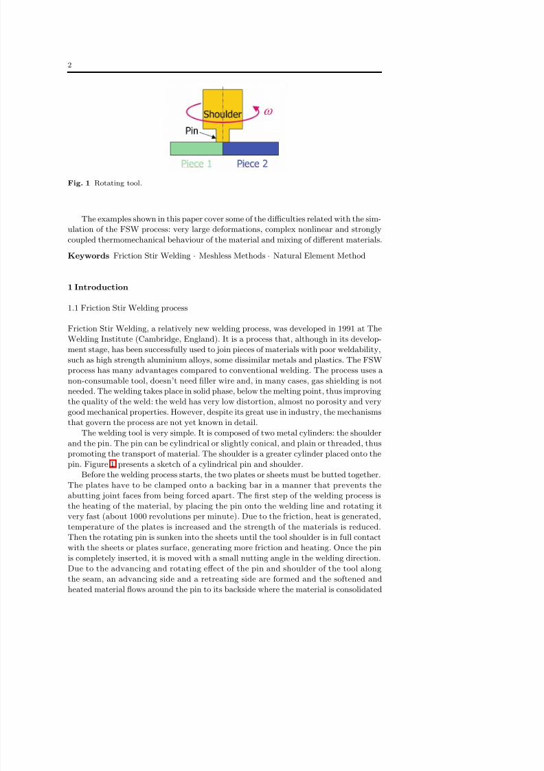
Fig. 1 Rotating tool.

The examples shown in this paper cover some of the difficulties related with the sim-ulation of the FSW process: very large deformations, complex nonlinear and strongly

coupled thermomechanical behaviour of the material and mixing of different materials.

Keywords Friction Stir Welding · Meshless Methods · Natural Element Method

1 Introduction

1.1 Friction Stir Welding process

Friction Stir Welding, a relatively new welding process, was developed in 1991 at The

Welding Institute (Cambridge, England). It is a process that, although in its develop-

ment stage, has been successfully used to join pieces of materials with poor weldability,

such as high strength aluminium alloys, some dissimilar metals and plastics. The FSWprocess has many advantages compared to conventional welding. The process uses a

non-consumable tool, doesn’t need filler wire and, in many cases, gas shielding is notneeded. The welding takes place in solid phase, below the melting point, thus improving

the quality of the weld: the weld has very low distortion, almost no porosity and verygood mechanical properties. However, despite its great use in industry, the mechanisms

that govern the process are not yet known in detail.

The welding tool is very simple. It is composed of two metal cylinders: the shoulder

and the pin. The pin can be cylindrical or slightly conical, and plain or threaded, thus

promoting the transport of material. The shoulder is a greater cylinder placed onto the

pin. Figure 1 presents a sketch of a cylindrical pin and shoulder.

Before the welding process starts, the two plates or sheets must be butted together.

The plates have to be clamped onto a backing bar in a manner that prevents the

abutting joint faces from being forced apart. The first step of the welding process is

the heating of the material, by placing the pin onto the welding line and rotating itvery fast (about 1000 revolutions per minute). Due to the friction, heat is generated,

temperature of the plates is increased and the strength of the materials is reduced.

Then the rotating pin is sunken into the sheets until the tool shoulder is in full contactwith the sheets or plates surface, generating more friction and heating. Once the pin

is completely inserted, it is moved with a small nutting angle in the welding direction.

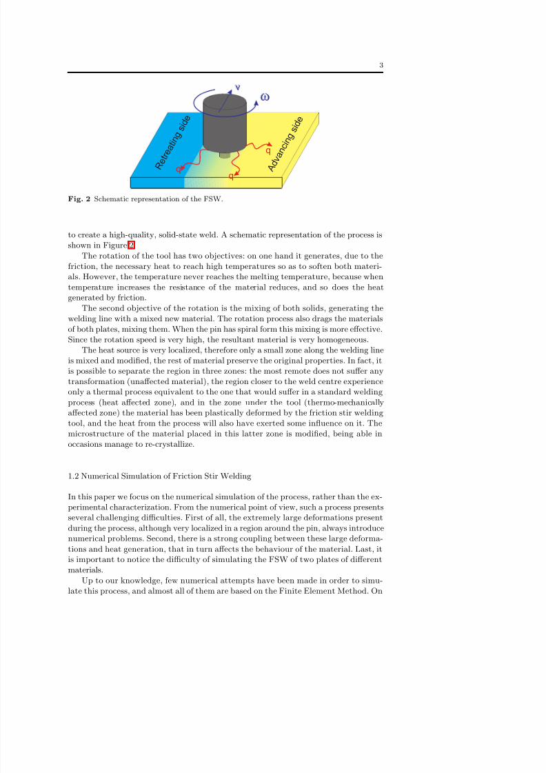
Due to the advancing and rotating effect of the pin and shoulder of the tool along

the seam, an advancing side and a retreating side are formed and the softened and

heated material flows around the pin to its backside where the material is consolidated





4

the first attempts [1] only the evolution of the temperature in the stationary phase

was simulated. The steady-state of the FSW process can be simulated easily usingEulerian approaches [2], including complex thermomechanical models, but the tran-

sient phase can not be solved using this method. In [3] a Lagrangian approach with

intensive remeshing is employed. Similar approaches have been employed in [4] and

[5]. Remeshing, however, is well-known as a potential source of numerical diffusion in

the results. Other authors use arbitrary Lagrangian Eulerian (ALE) formulations [6],

studying and taking into account the diffusion related to the mapping inherent to thisnumerical method. Extended finite element methods (X-FEM) could also be employed

to this end, see for instance [7].

In this paper we employ a somewhat different approach based on the use of meshless

methods. Meshless methods allow for a Lagrangian description of the motion, while

avoiding the need for remeshing (a review of the state of the art in meshless methods

can be consulted in [8]). Thus, the nodes, that in our implementation transport allthe variables linked to material’s history, remain the same throughout the simulation.

Mappings between old and new meshes are not necessary and hence the avoidance of numerical diffusion.

Among the many meshless methods available nowadays, we have chosen the Natural

Element Method [9] [10]. It possesses some noteworthy advantages over other meshless

methods that will be described on the following section.

2 The Natural Element Method

Essentially, the NEM is a Galerkin procedure that relies on natural neighbour interpo-

lation to construct the trial and test functions characteristic of this method. Prior tothe definition of these interpolation functions, it is necessary to introduce some basic

geometrical entities that are needed for further developments.

2.1 Voronoi/Dirichlet diagrams

Consider a model composed by a cloud of points N = n1, n2, . . . , nm ⊂ Rd, for

which there is a unique decomposition of the space into regions such that each point

within these regions is closer to the node to which the region is associated than to anyother in the cloud. This kind of space decomposition is called a Voronoi diagram (also

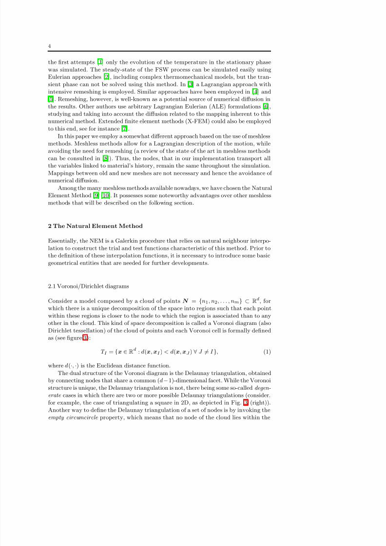
Dirichlet tessellation) of the cloud of points and each Voronoi cell is formally definedas (see figure 3):

T I = x ∈ Rd : d(x,xI ) < d(x,xJ ) ∀ J = I , (1)

where d(·, ·) is the Euclidean distance function.

The dual structure of the Voronoi diagram is the Delaunay triangulation, obtained

by connecting nodes that share a common (d− 1)-dimensional facet. While the Voronoistructure is unique, the Delaunay triangulation is not, there being some so-called degen-

erate cases in which there are two or more possible Delaunay triangulations (consider,

for example, the case of triangulating a square in 2D, as depicted in Fig. 3 (right)).

Another way to define the Delaunay triangulation of a set of nodes is by invoking theempty circumcircle property, which means that no node of the cloud lies within the



5

Fig. 3 Delaunay triangulation and Voronoi diagram of a cloud of points.

circle covering a Delaunay triangle. Two nodes sharing a facet of their Voronoi cell are

called natural neighbours and hence the name of the technique.

Equivalently, the second-order Voronoi diagram of the cloud is defined as

T IJ = x ∈ Rd : d(x,xI ) < d(x,xJ ) < d(x,xK ) ∀ J = I = K . (2)

Based on these definitions, different natural neighbour interpolation schemes have

been proposed. In this paper we have used the so-called Sibson interpolation for veloc-ities and Thiessen interpolation for pressure, following the analysis done in [11].

2.2 Thiessen interpolation

The simplest of the natural neighbour-based interpolants is the so-called Thiessen’s

interpolant [12]. Its interpolating functions are defined as

ψI (x) =

(1 if x ∈ T I 0 elsewhere

. (3)

The Thiessen interpolant is a piece-wise constant function, defined over each Voronoi

cell. It defines a method of interpolation often referred to as nearest neighbour inter-polation, since a point is given a value defined by its nearest neighbour. Although it is

obviously not valid for the solution of second-order partial differential equations, it can

be used to interpolate the pressure in formulations arising from Hellinger-Reissner-like

mixed variational principles, as proved in [11].

2.3 Sibson’s interpolation

The most extended natural neighbour interpolation method is the Sibson interpolant

[13] [14]. Consider the introduction of the point x in the cloud of nodes. Due to thisintroduction, the Voronoi diagram will be altered, affecting the Voronoi cells of the

natural neighbours of x. Sibson [13] defined the natural neighbour coordinates of apoint x with respect to one of its neighbours I as the ratio of the cell T I that is

transferred to T x when adding x to the initial cloud of points to the total volumeof T x. In other words, if κ(x) and κI (x) are the Lebesgue measures of T x and T xI respectively, the natural neighbour coordinates of x with respect to the node I is

defined as

φI (x) = κI (x)

κ(x) . (4)



6

x1

2

3

4

5

6

7

a

b c

de

f

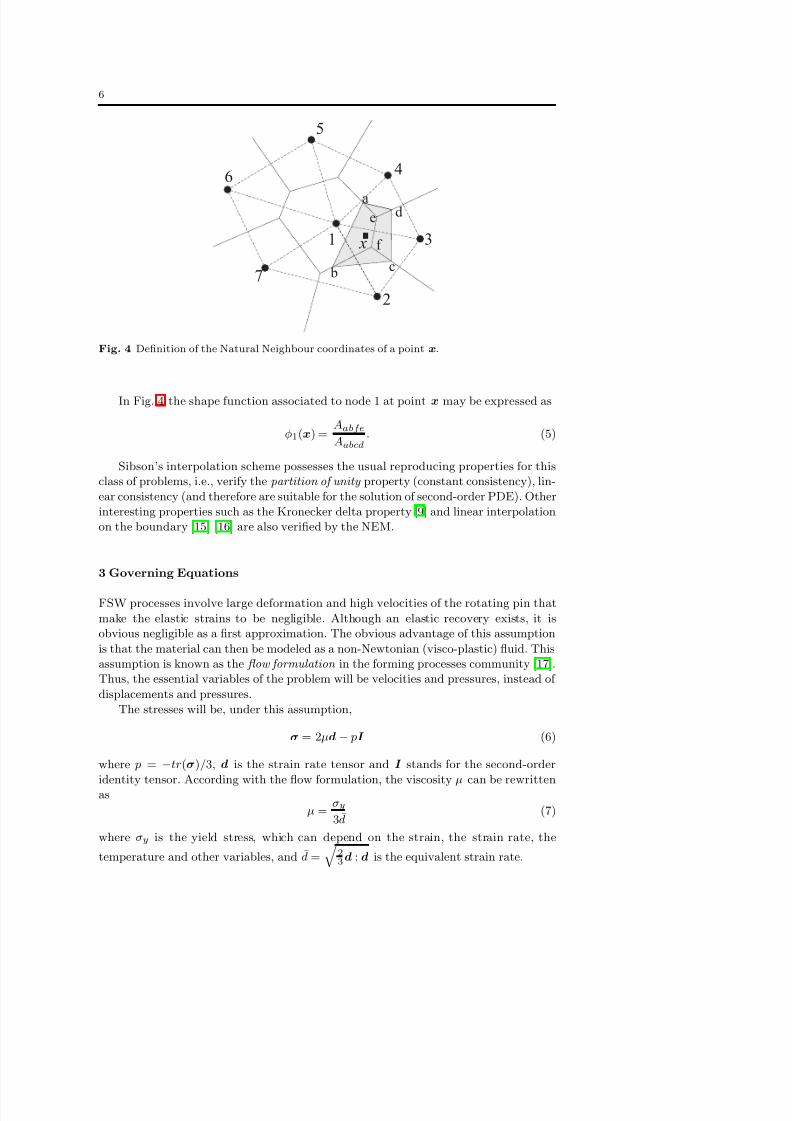
Fig. 4 Definition of the Natural Neighbour coordinates of a point x.

In Fig. 4 the shape function associated to node 1 at point x may be expressed as

φ1(x) = Aabfe

Aabcd. (5)

Sibson’s interpolation scheme possesses the usual reproducing properties for thisclass of problems, i.e., verify the partition of unity property (constant consistency), lin-

ear consistency (and therefore are suitable for the solution of second-order PDE). Other

interesting properties such as the Kronecker delta property [9] and linear interpolationon the boundary [15] [16] are also verified by the NEM.

3 Governing Equations

FSW processes involve large deformation and high velocities of the rotating pin that

make the elastic strains to be negligible. Although an elastic recovery exists, it isobvious negligible as a first approximation. The obvious advantage of this assumption

is that the material can then be modeled as a non-Newtonian (visco-plastic) fluid. Thisassumption is known as the flow formulation in the forming processes community [17].Thus, the essential variables of the problem will be velocities and pressures, instead of

displacements and pressures.

The stresses will be, under this assumption,

σ = 2µd − pI (6)

where p = −tr(σ)/3, d is the strain rate tensor and I stands for the second-order

identity tensor. According with the flow formulation, the viscosity µ can be rewrittenas

µ = σy

3d (7)

where σy is the yield stress, which can depend on the strain, the strain rate, the

temperature and other variables, and d =q

2

3d : d is the equivalent strain rate.



7

We consider, for the plates being welded, the balance of momentum equations

without inertia and mass terms and the assumed incompressibility of a von Mises-likeflow:

∇σ = 0, ∇v = 0 (8)

where v represents the velocity field. Velocities are interpolated by means of the Sibsonshape functions, while pressures are considered constant over the whole Voronoi cellassociated to each node and thus interpolated with Thiessen shape functions.

Temperature is also an essential variable in the problem. To study the evolutionand distribution of temperatures, the rigid-plastic material equations are coupled with

the following heat transfer equations:

∇(k∇T ) + r − (ρc p T ) = 0 (9)

where k denotes the thermal conductivity, r the heat generation rate, ρ the specific

density and c p the specific heat of the metal. The rate of heat generation due to plasticdeformation is calculated as

r = β σ : d (10)

where β represents the fraction of mechanical energy transformed to heat and is as-sumed to be 0.9 [18].

Together with these equations, appropriate boundary conditions are considered:

σ · n = t on Γ t (11)

v = v on Γ v (12)

where Γ t and Γ v represent, respectively, the part of the boundary Γ = ∂ Ω where trac-

tions and velocities are prescribed. In addition, along the boundary, either temperatureor heat flux is prescribed.

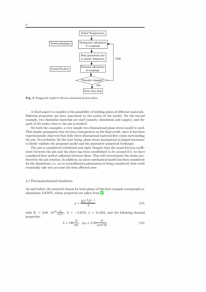
The coupling has been made through a block-iterative semi-implicit method, to-gether with a fixed-point algorithm to treat the non-linear coupling (see figure 5). This

strategy has also been employed successfully in previous works of the authors [19].

Numerical integration of the weak form of the problems given by Eqs. (8) and (9) isachieved through the use of three-point quadrature rules on the Delaunay trianglesfor simplicity, although more sophisticated techniques, such as Stabilized Conforming

Nodal Integration (SCNI), could equally be used.

4 Examples and numerical results

The aim of the examples shown here is to check the ability of the NEM to solve different

difficulties related to the simulation of the FSW process.

The first aspect to consider is the extremely high strain which would distort themesh if the simulation is done using FEM. At the beginning of the simulations, a

more or less regular cloud of nodes is used, but the same cloud of nodes, which will

become very irregularly distributed, will be used during the whole process. An updatedLagrangian procedure is used in all simulations.

The nonlinear thermomechanical behaviour is another source of complexity. Then,

on the first example real material properties, corresponding to aluminium AA7075, are

used to check the robustness of the NEM procedure. The simulation will also show the

influence of the temperature evolution on the mechanical properties.



8

Fig. 5 Staggered implicit thermo-mechanical procedure.

A third aspect to consider is the possibility of welding plates of different materials.

Material properties are here associated to the nodes of the model. On the secondexample, two dissimilar materials are used (namely, aluminium and copper), and the

path of the nodes close to the pin is studied.

On both the examples, a very simple two-dimensional plane stress model is used.This simple assumption has obvious consequences on the final result, since it has been

experimentally observed that fully three-dimensional material flow exists surrounding

the pin. Nevertheless, for the time being, plane stress assumption is judged necessary

to firstly validate the proposed model and the associated numerical technique.

The pin is considered cylindrical and rigid. Despite that the usual friction coeffi-

cient between the pin and the sheet has been established to be around 0.5, we have

considered here perfect adhesion between them. This will overestimate the strain pro-

duced by the pin rotation. In addition, no micro-mechanical model has been consideredfor the aluminium, i.e., no re-crystallization phenomena is being considered, that could

eventually take into account the heat affected zone.

4.1 Thermomechanical simulation

As said before, the material chosen for both plates of this first example corresponds to

aluminium AA7075, whose properties are taken from [4]:

µ =

KT A dn−1

3 (13)

with K = 2.69 · 1010 N mm2 , A = −3.3155, n = 0.1324, and the following thermal

properties:

k = 180 N

sK , ρc p = 2.39

N

mm2K (14)



9

X

Y

-6 -4 -2 0 2 4 6

-6

-4

-2

0

2

4

6

v

w

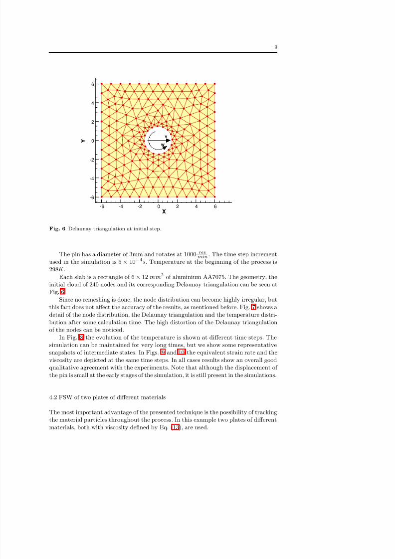
Fig. 6 Delaunay triangulation at initial step.

The pin has a diameter of 3mm and rotates at 1000 revmin . The time step increment

used in the simulation is 5 × 10−4s. Temperature at the beginning of the process is298K .

Each slab is a rectangle of 6 × 12 mm2 of aluminium AA7075. The geometry, theinitial cloud of 240 nodes and its corresponding Delaunay triangulation can be seen at

Fig. 6.Since no remeshing is done, the node distribution can become highly irregular, but

this fact does not affect the accuracy of the results, as mentioned before. Fig. 7 shows a

detail of the node distribution, the Delaunay triangulation and the temperature distri-

bution after some calculation time. The high distortion of the Delaunay triangulationof the nodes can be noticed.

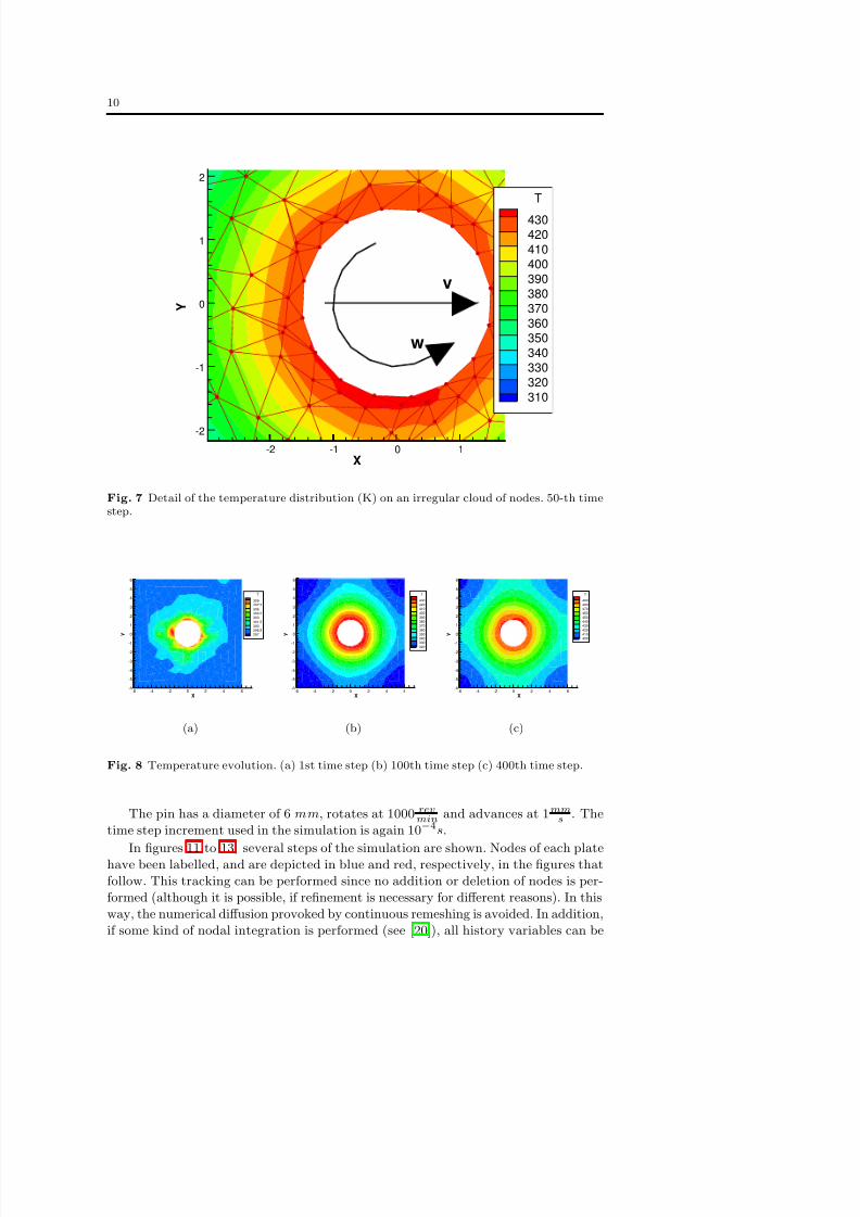
In Fig. 8 the evolution of the temperature is shown at different time steps. Thesimulation can be maintained for very long times, but we show some representative

snapshots of intermediate states. In Figs. 9 and 10 the equivalent strain rate and the

viscosity are depicted at the same time steps. In all cases results show an overall goodqualitative agreement with the experiments. Note that although the displacement of

the pin is small at the early stages of the simulation, it is still present in the simulations.

4.2 FSW of two plates of different materials

The most important advantage of the presented technique is the possibility of tracking

the material particles throughout the process. In this example two plates of different

materials, both with viscosity defined by Eq. (13), are used.



10

X

Y

-2 -1 0 1

-2

-1

0

1

2

T

430

420

410

400

390

380

370

360

350

340

330

320

310

v

w

Fig. 7 Detail of the temperature distribution (K) on an irregular cloud of nodes. 50-th timestep.

X

Y

-6 -4 -2 0 2 4 6-6

-5

-4

-3

-2

-1

0

1

2

3

4

5

6

T

309

307.5

306

304.5

303

301.5

300

298.5

297

(a)

X

Y

-6 -4 -2 0 2 4 6-6

-5

-4

-3

-2

-1

0

1

2

3

4

5

6

T

430

420

410

400

390

380

370

360

350

340

330

320

(b)

X

Y

-6 -4 -2 0 2 4 6-6

-5

-4

-3

-2

-1

0

1

2

3

4

5

6

T

490

480

470

460

450

440

430

420

410

400

(c)

Fig. 8 Temperature evolution. (a) 1st time step (b) 100th time step (c) 400th time step.

The pin has a diameter of 6 mm, rotates at 1000 revmin and advances at 1mms . The

time step increment used in the simulation is again 10−4s.

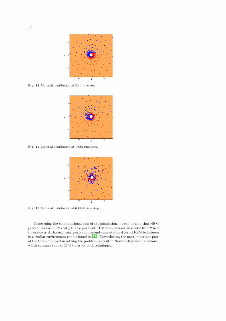
In figures 11 to 13, several steps of the simulation are shown. Nodes of each platehave been labelled, and are depicted in blue and red, respectively, in the figures that

follow. This tracking can be performed since no addition or deletion of nodes is per-

formed (although it is possible, if refinement is necessary for different reasons). In this

way, the numerical diffusion provoked by continuous remeshing is avoided. In addition,

if some kind of nodal integration is performed (see [20]), all history variables can be



11

X

Y

-6 -4 -2 0 2 4 6-6

-5

-4

-3

-2

-1

0

1

2

3

4

5

6

d

180

170

160

150

140

130

120

110

100

90

80

70

60

50

40

30

20

10

(a)

X

Y

-6 -4 -2 0 2 4 6-6

-5

-4

-3

-2

-1

0

1

2

3

4

5

6

d

180

170

160

150

140

130

120

110

100

90

80

70

60

50

40

30

20

10

(b)

X

Y

-6 -4 -2 0 2 4 6-6

-5

-4

-3

-2

-1

0

1

2

3

4

5

6

d

180

170

160

150

140

130

120

110

100

90

80

70

60

50

40

30

20

10

(c)

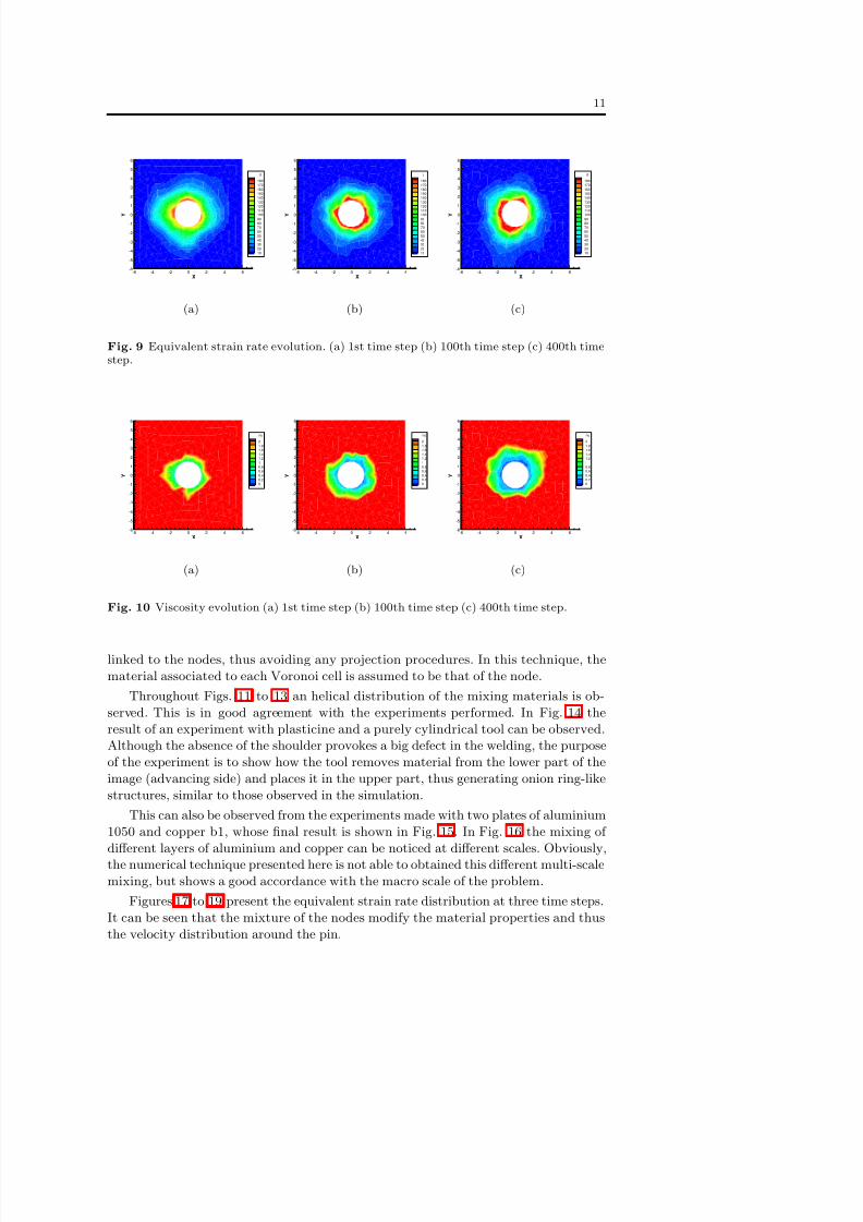
Fig. 9 Equivalent strain rate evolution. (a) 1st time step (b) 100th time step (c) 400th timestep.

X

Y

-6 -4 -2 0 2 4 6-6

-5

-4

-3

-2

-1

0

1

2

3

4

5

6

nu

2

1.8

1.6

1.4

1.2

1

0.8

0.6

0.4

0.2

0

(a)

X

Y

-6 -4 -2 0 2 4 6-6

-5

-4

-3

-2

-1

0

1

2

3

4

5

6

nu

2

1.8

1.6

1.4

1.2

1

0.8

0.6

0.4

0.2

0

(b)

X

Y

-6 -4 -2 0 2 4 6-6

-5

-4

-3

-2

-1

0

1

2

3

4

5

6

nu

2

1.8

1.6

1.4

1.2

1

0.8

0.6

0.4

0.2

0

(c)

Fig. 10 Viscosity evolution (a) 1st time step (b) 100th time step (c) 400th time step.

linked to the nodes, thus avoiding any projection procedures. In this technique, the

material associated to each Voronoi cell is assumed to be that of the node.

Throughout Figs. 11 to 13 an helical distribution of the mixing materials is ob-

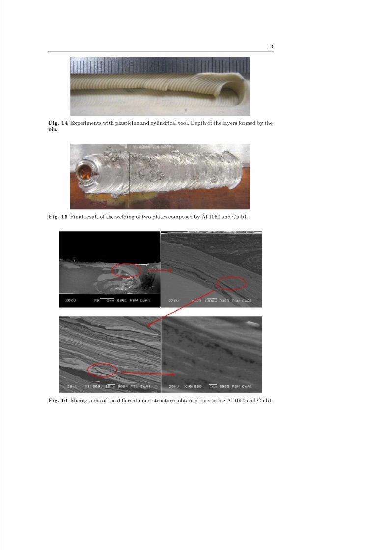
served. This is in good agreement with the experiments performed. In Fig. 14 the

result of an experiment with plasticine and a purely cylindrical tool can be observed.Although the absence of the shoulder provokes a big defect in the welding, the purpose

of the experiment is to show how the tool removes material from the lower part of the

image (advancing side) and places it in the upper part, thus generating onion ring-like

structures, similar to those observed in the simulation.

This can also be observed from the experiments made with two plates of aluminium

1050 and copper b1, whose final result is shown in Fig. 15. In Fig. 16 the mixing of

different layers of aluminium and copper can be noticed at different scales. Obviously,the numerical technique presented here is not able to obtained this different multi-scale

mixing, but shows a good accordance with the macro scale of the problem.

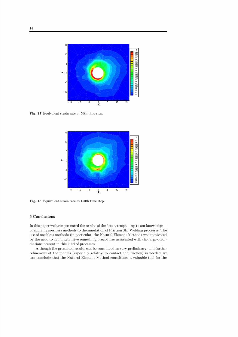
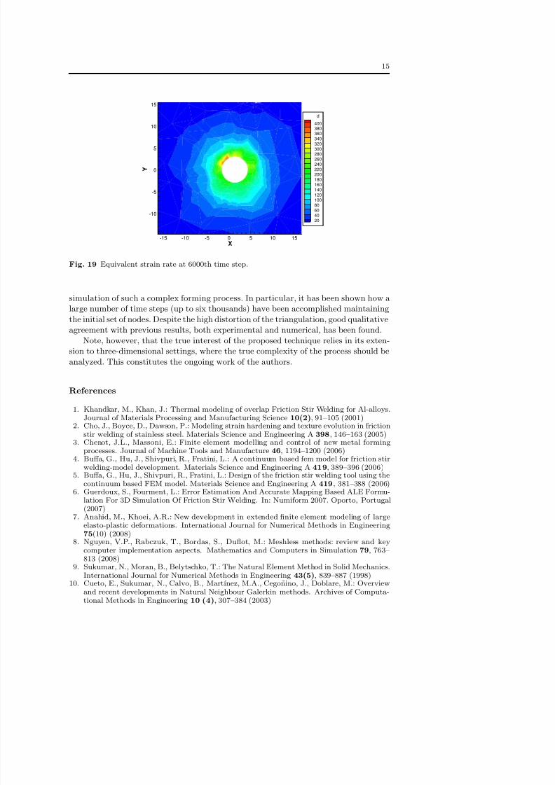
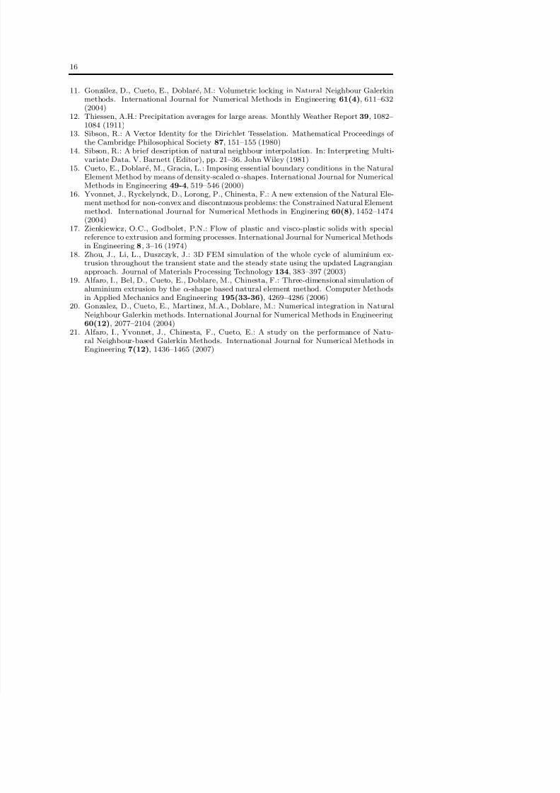
Figures 17 to 19 present the equivalent strain rate distribution at three time steps.

It can be seen that the mixture of the nodes modify the material properties and thus

the velocity distribution around the pin.





13

Fig. 14 Experiments with plasticine and cylindrical tool. Depth of the layers formed by thepin.

Fig. 15 Final result of the welding of two plates composed by Al 1050 and Cu b1.

Fig. 16 Micrographs of the different microstructures obtained by stirring Al 1050 and Cu b1.



14

X

Y

-15 -10 -5 0 5 10 15

-10

-5

0

5

10

15

d

400

380

360

340

320

300

280

260

240

220

200

180

160

140

120

100

80

60

40

20

Fig. 17 Equivalent strain rate at 50th time step.

X

Y

-15 -10 -5 0 5 10 15

-10

-5

0

5

10

15

d

400

380

360

340

320

300

280

260

240

220

200

180

160

140

120

100

80

60

40

20


5 Conclusions

In this paper we have presented the results of the first attempt —up to our knowledge—

of applying meshless methods to the simulation of Friction Stir Welding processes. The

use of meshless methods (in particular, the Natural Element Method) was motivatedby the need to avoid extensive remeshing procedures associated with the large defor-mations present in this kind of processes.

Although the presented results can be considered as very preliminary, and further

refinement of the models (especially relative to contact and friction) is needed, we

can conclude that the Natural Element Method constitutes a valuable tool for the



15

X

Y

-15 -10 -5 0 5 10 15

-10

-5

0

5

10

15

d

400

380

360

340

320

300

280

260

240

220

200

180

160

140

120

100

80

60

40

20


simulation of such a complex forming process. In particular, it has been shown how alarge number of time steps (up to six thousands) have been accomplished maintaining

the initial set of nodes. Despite the high distortion of the triangulation, good qualitative

agreement with previous results, both experimental and numerical, has been found.

Note, however, that the true interest of the proposed technique relies in its exten-sion to three-dimensional settings, where the true complexity of the process should be

analyzed. This constitutes the ongoing work of the authors.

References

1. Khandkar, M., Khan, J.: Thermal modeling of overlap Friction Stir Welding for Al-alloys.Journal of Materials Processing and Manufacturing Science 10(2), 91–105 (2001)2. Cho, J., Boyce, D., Dawson, P.: Modeling strain hardening and texture evolution in friction

stir welding of stainless steel. Materials Science and Engineering A 398, 146–163 (2005)3. Chenot, J.L., Massoni, E.: Finite element modelling and control of new metal forming

processes. Journal of Machine Tools and Manufacture 46, 1194–1200 (2006)4. Buffa, G., Hu, J., Shivpuri, R., Fratini, L.: A continuum based fem model for friction stir

welding-model development. Materials Science and Engineering A 419, 389–396 (2006)5. Buffa, G., Hu, J., Shivpuri, R., Fratini, L.: Design of the friction stir welding tool using the

continuum based FEM model. Materials Science and Engineering A 419 , 381–388 (2006)6. Guerdoux, S., Fourment, L.: Error Estimation And Accurate Mapping Based ALE Formu-

lation For 3D Simulation Of Friction Stir Welding. In: Numiform 2007. Oporto, Portugal(2007)

7. Anahid, M., Khoei, A.R.: New development in extended finite element modeling of largeelasto-plastic deformations. International Journal for Numerical Methods in Engineering75(10) (2008)

8. Nguyen, V.P., Rabczuk, T., Bordas, S., Duflot, M.: Meshless methods: review and key

computer implementation aspects. Mathematics and Computers in Simulation 79, 763–813 (2008)

9. Sukumar, N., Moran, B., Belytschko, T.: The Natural Element Method in Solid Mechanics.International Journal for Numerical Methods in Engineering 43(5), 839–887 (1998)

10. Cueto, E., Sukumar, N., Calvo, B., Martınez, M.A., Cegonino, J., Doblare, M.: Overviewand recent developments in Natural Neighbour Galerkin methods. Archives of Computa-tional Methods in Engineering 10 (4), 307–384 (2003)



16

11. Gonzalez, D., Cueto, E., Doblare, M.: Volumetric locking in Natural Neighbour Galerkinmethods. International Journal for Numerical Methods in Engineering 61(4), 611–632(2004)

12. Thiessen, A.H.: Precipitation averages for large areas. Monthly Weather Report 39, 1082–1084 (1911)

13. Sibson, R.: A Vector Identity for the Dirichlet Tesselation. Mathematical Proceedings of the Cambridge Philosophical Society 87, 151–155 (1980)

14. Sibson, R.: A brief description of natural neighbour interpolation. In: Interpreting Multi-variate Data. V. Barnett (Editor), pp. 21–36. John Wiley (1981)

15. Cueto, E., Doblare, M., Gracia, L.: Imposing essential boundary conditions in the NaturalElement Method by means of density-scaled α-shapes. International Journal for NumericalMethods in Engineering 49-4, 519–546 (2000)

16. Yvonnet, J., Ryckelynck, D., Lorong, P., Chinesta, F.: A new extension of the Natural Ele-ment method for non-convex and discontnuous problems: the Constrained Natural Elementmethod. International Journal for Numerical Methods in Enginering 60(8), 1452–1474(2004)

17. Zienkiewicz, O.C., Godbolet, P.N.: Flow of plastic and visco-plastic solids with specialreference to extrusion and forming processes. International Journal for Numerical Methodsin Engineering 8, 3–16 (1974)

18. Zhou, J., Li, L., Duszczyk, J.: 3D FEM simulation of the whole cycle of aluminium ex-trusion throughout the transient state and the steady state using the updated Lagrangianapproach. Journal of Materials Processing Technology 134, 383–397 (2003)

19. Alfaro, I., Bel, D., Cueto, E., Doblare, M., Chinesta, F.: Three-dimensional simulation of aluminium extrusion by the α-shape based natural element method. Computer Methodsin Applied Mechanics and Engineering 195(33-36), 4269–4286 (2006)

20. Gonzalez, D., Cueto, E., Martinez, M.A., Doblare, M.: Numerical integration in NaturalNeighbour Galerkin methods. International Journal for Numerical Methods in Engineering60(12), 2077–2104 (2004)

21. Alfaro, I., Yvonnet, J., Chinesta, F., Cueto, E.: A study on the performance of Natu-ral Neighbour-based Galerkin Methods. International Journal for Numerical Methods inEngineering 7(12), 1436–1465 (2007)

Documents

Numerical Simulation of Friction Stir Welding by Natural Element Methods Alfaro