Embed Size (px)
Citation preview

Numerical Results for shear-lock free finite elements based on Mindlin-Reissner plate and Timoshenko beam theories
Plate Elements N x N Mesh Size (Full Plate) Exact Solution Srinivasa Rao and AK Rao and Theory of Plates and Shells CF Convergence Factor ASR Aspect Ratio MR_FE_1 Finite Elements based on Mindlin-Reissner theory using new MR_FE_2 shape functions MR_FE_3 MR_FE_4 Material: E=1.092E06; 𝜐 = 0.3; Geometry: Square plate a=10.0;
h=2.0, 1.4, 1.0, 0.5;
Type of plate Simply supported (SS) Load: UDL=10.0 Timoshenko beam elements N Number of Elements (Full beam) Exact Solution Theory of Elasticity CF Convergence Factor ASR Aspect Ratio Timo_FE_1 Finite Elements based on Timoshenko beam theory using new Timo_FE_2 shape functions Timo_FE_3 Timo_FE_4 Material: 29,000; 𝜐 = 0.3; Geometry: L=5,10, 25,100, 200, 400;
h=1.0; b=1.0; Load: Concentrated Load q=100.0 and UDL=10.0 Higher order beam elements (capable of accurately predicting three dimensional stresses) based on the higher order shear deformation theories developed by me HFE_1 - based on Lagrangian polynomials HFE_3 - based on Lagrangian polynomials FE_NSF_1 - based on new shape functions FE_NSF_3 - based on new shape functions
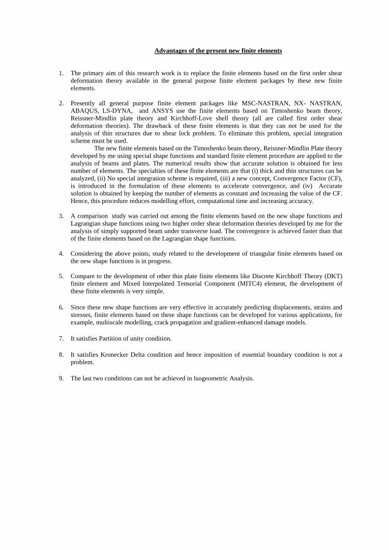
Advantages of the present new finite elements
1. The primary aim of this research work is to replace the finite elements based on the first order shear deformation theory available in the general purpose finite element packages by these new finite elements.
2. Presently all general purpose finite element packages like MSC-NASTRAN, NX- NASTRAN,
ABAQUS, LS-DYNA, and ANSYS use the finite elements based on Timoshenko beam theory, Reissner-Mindlin plate theory and Kirchhoff-Love shell theory (all are called first order shear deformation theories). The drawback of these finite elements is that they can not be used for the analysis of thin structures due to shear lock problem. To eliminate this problem, special integration scheme must be used.
The new finite elements based on the Timoshenko beam theory, Reissner-Mindlin Plate theory developed by me using special shape functions and standard finite element procedure are applied to the analysis of beams and plates. The numerical results show that accurate solution is obtained for less number of elements. The specialties of these finite elements are that (i) thick and thin structures can be analyzed, (ii) No special integration scheme is required, (iii) a new concept, Convergence Factor (CF), is introduced in the formulation of these elements to accelerate convergence, and (iv) Accurate solution is obtained by keeping the number of elements as constant and increasing the value of the CF. Hence, this procedure reduces modelling effort, computational time and increasing accuracy.
3. A comparison study was carried out among the finite elements based on the new shape functions and
Lagrangian shape functions using two higher order shear deformation theories developed by me for the analysis of simply supported beam under transverse load. The convergence is achieved faster than that of the finite elements based on the Lagrangian shape functions.
4. Considering the above points, study related to the development of triangular finite elements based on the new shape functions is in progress.
5. Compare to the development of other thin plate finite elements like Discrete Kirchhoff Theory (DKT) finite element and Mixed Interpolated Tensorial Component (MITC4) element, the development of these finite elements is very simple.
6. Since these new shape functions are very effective in accurately predicting displacements, strains and stresses, finite elements based on these shape functions can be developed for various applications, for example, multiscale modelling, crack propagation and gradient-enhanced damage models.
7. It satisfies Partition of unity condition.
8. It satisfies Kronecker Delta condition and hence imposition of essential boundary condition is not a problem.
9. The last two conditions can not be achieved in Isogeometric Analysis.
ErroCantileve
or in deflecAs
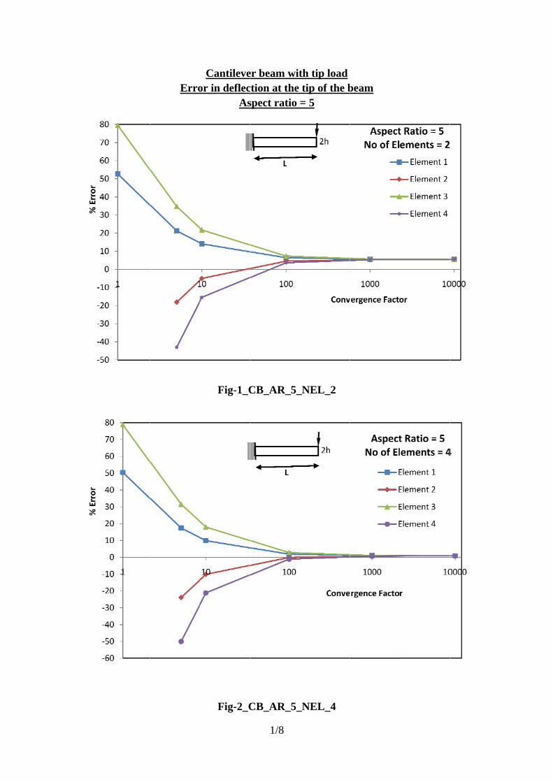
Fig-1_C
Fig-2_C
1/8
er beam witction at the spect ratio
CB_AR_5_
CB_AR_5_
th tip loadtip of the b= 5
_NEL_2
_NEL_4
beam
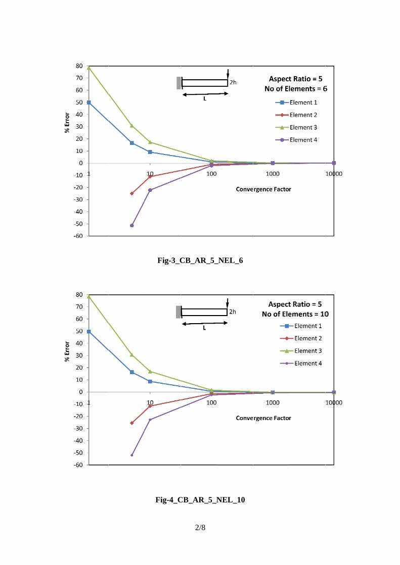
Fig-3_C
Fig-4_C
2/8
CB_AR_5_
CB_AR_5_N
_NEL_6
NEL_10
ErroCantileve
or in deflecAsp
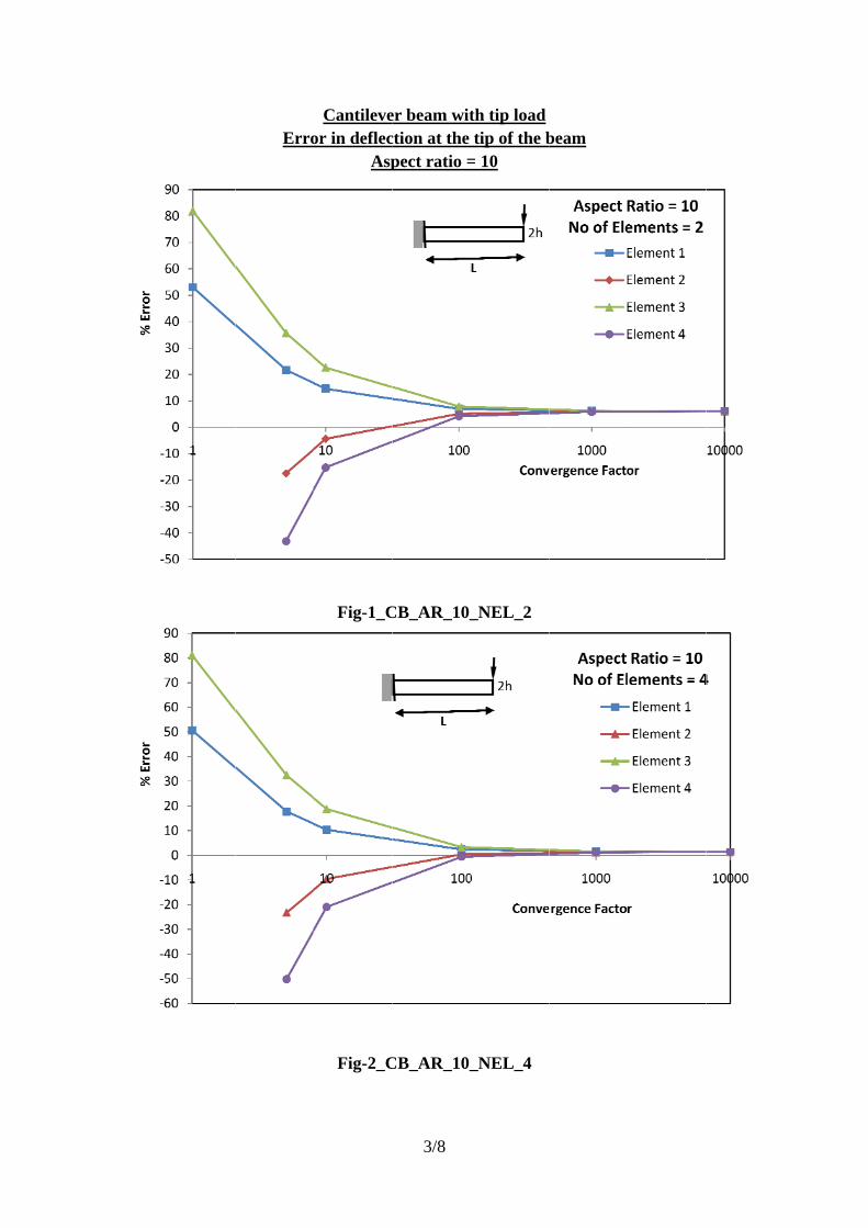
Fig-1_C
Fig-2_C
3/8
er beam witction at the pect ratio =
CB_AR_10_
CB_AR_10_
th tip loadtip of the b
= 10
_NEL_2
_NEL_4
beam
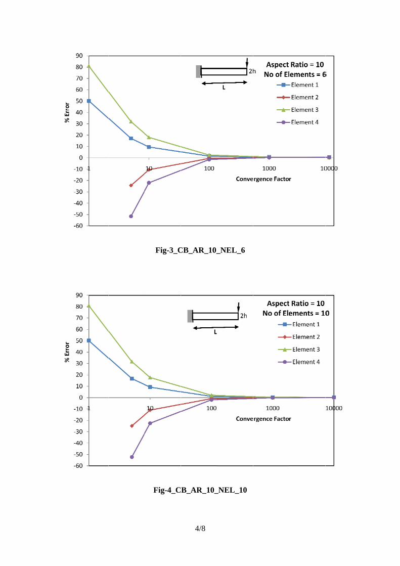
Fig-3_C
Fig-4_C
4/8
CB_AR_10_
B_AR_10_
_NEL_6
_NEL_10
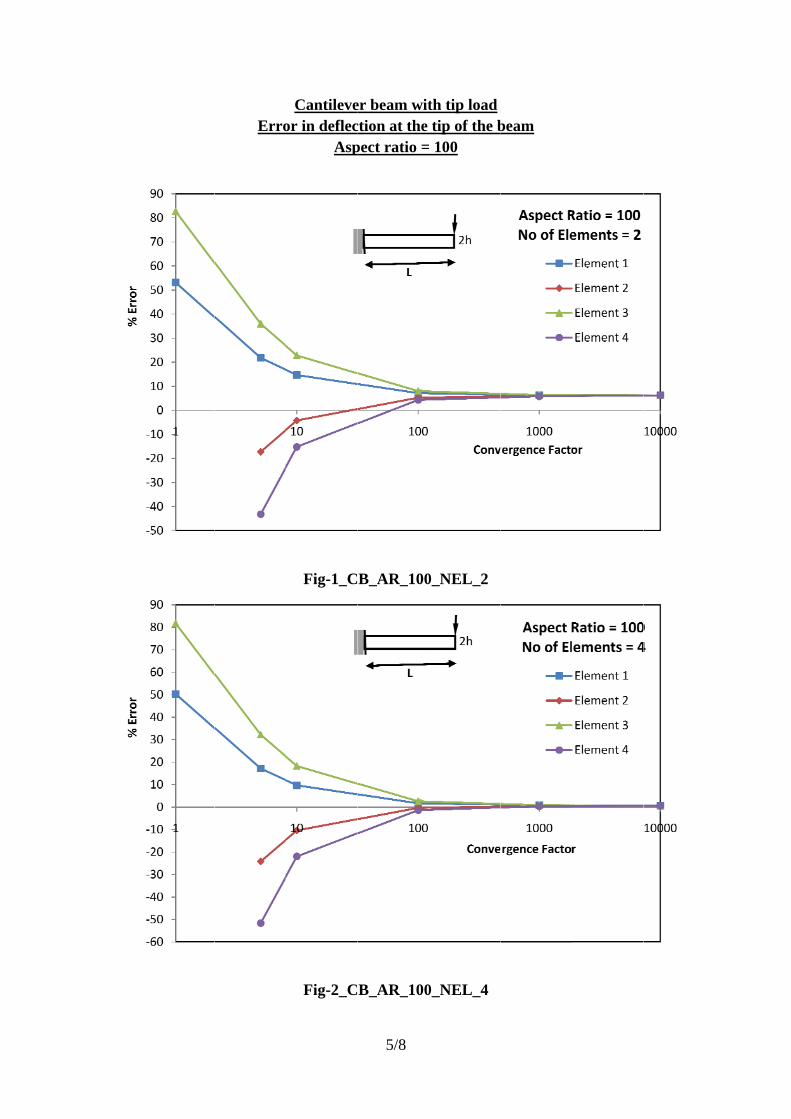
ErroCantileve
or in deflecAsp
Fig-1_C
Fig-2_C
5/8
er beam witction at the pect ratio =
B_AR_100
B_AR_100
th tip loadtip of the b
= 100
0_NEL_2
0_NEL_4
beam
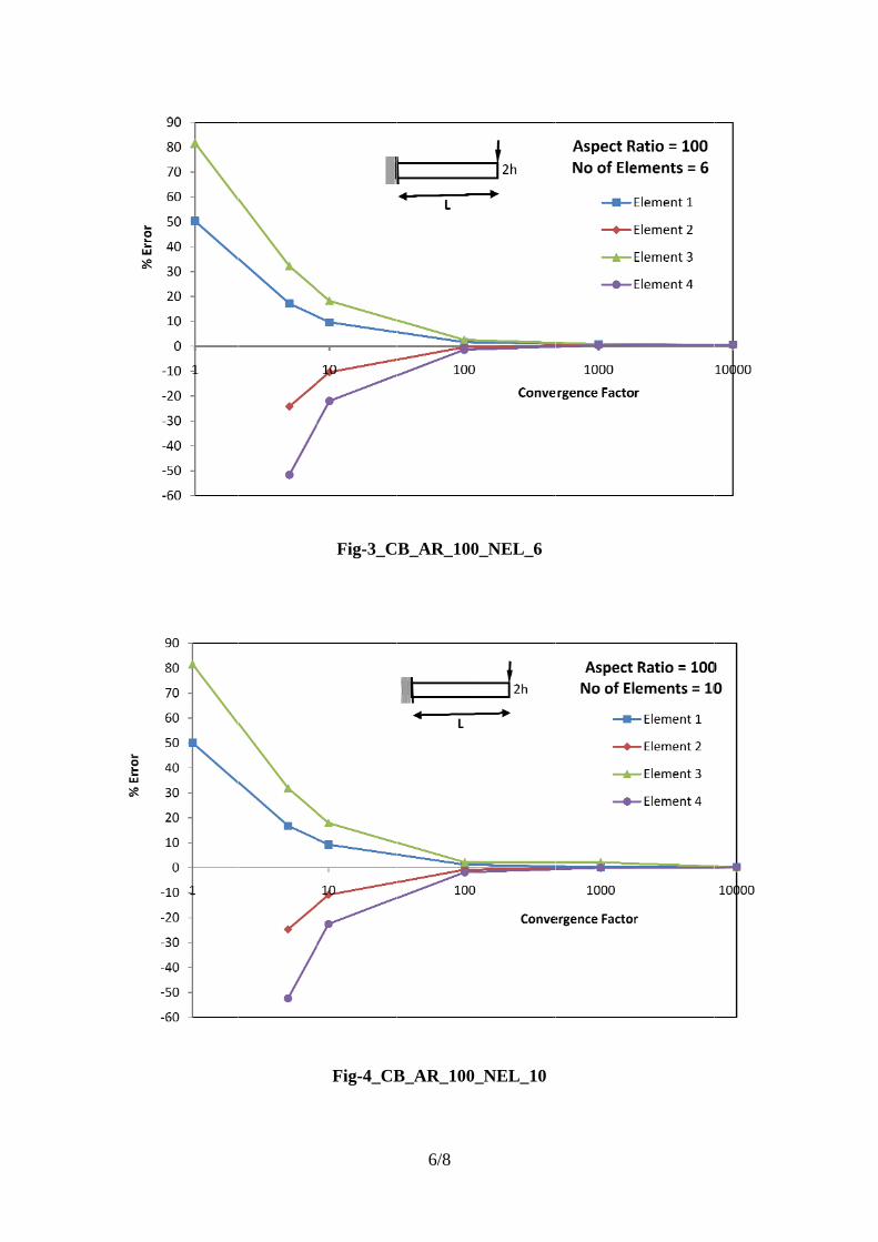
Fig-3_C
Fig-4_CB
6/8
B_AR_100
B_AR_100_
0_NEL_6
_NEL_10
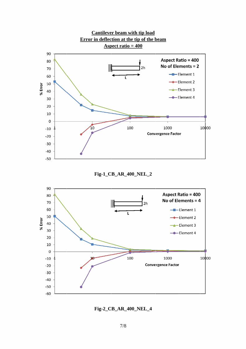
ErroCantileve
or in deflecAsp
Fig-1_C
Fig-2_C
7/8
er beam witction at the pect ratio =
B_AR_400
B_AR_400
th tip loadtip of the b
= 400
0_NEL_2
0_NEL_4
beam
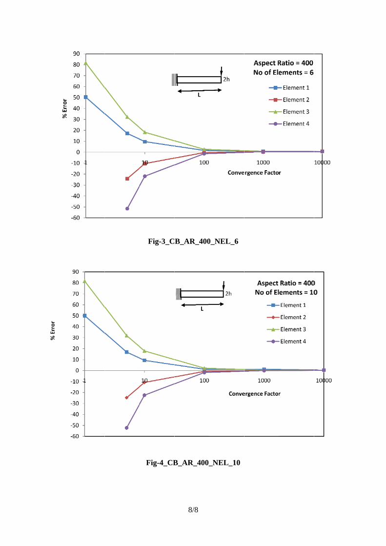
Fig-3_C
Fig-4_CB
8/8
B_AR_400
B_AR_400_
0_NEL_6
_NEL_10
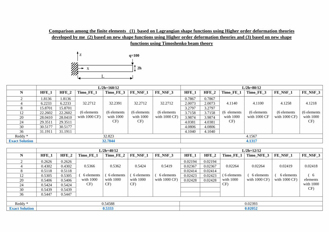
Comparison among the finite elements (1) based on Lagrangian shape functions using Higher order deformation theories developed by me (2) based on new shape functions using Higher order deformation theories and (3) based on new shape
functions using Timoshenko beam theory
L/2h=40/12 L/2h=12/12 N HFE_1 HFE_2 Timo_FE_1 Timo_FE_2 FE_NSF_1 FE_NSF_3 HFE_1 HFE_2 Timo_FE_1 Timo_NFE_3 FE_NSF_1 FE_NSF_3
2 0.2626 0.2626 0.5366
( 6 elements
with 1000 CF)
0.5362
( 6 elements with 1000 CF)
0.5424
( 6 elements with 1000 CF)
0.5419
( 6 elements with 1000 CF)
0.02194 0.02194 0.02264
( 6 elements with 1000 CF)
0.02264
( 6 elements with 1000 CF)
0.02419
( 6 elements with 1000 CF)
0.02418
( 6
elements with 1000
CF)
4 0.4302 0.4302 0.02367 0.02367 8 0.5118 0.5118 0.02414 0.02414
12 0.5305 0.5305 0.02423 0.02423 20 0.5406 0.5406 0.02428 0.02428 24 0.5424 0.5424 30 0.5439 0.5439 36 0.5447 0.5447
Reddy * 0.54588 0.02393
Exact Solution 0.5333 0.02052
L/2h=160/12 L/2h=80/12 N HFE_1 HFE_2 Timo_FE_1 Timo_FE_3 FE_NSF_1 FE_NSF_3 HFE_1 HFE_2 Timo_FE_1 Timo_FE_3 FE_NSF_1 FE_NSF_3
2 1.8136 1.8136 32.2712
(6 elements
with 1000 CF)
32.2391
(6 elements with 1000
CF)
32.2712
(6 elements with 1000
CF)
32.2712
(6 elements
with 1000 CF)
0.7867 0.7867 4.1140
(6 elements with 1000
CF)
4.1100
(6 elements
with 1000 CF
4.1258
(6 elements
with 1000 CF)
4.1218
(6 elements with 1000
CF)
4 6.2233 6.2233 2.0073 2.0073 8 15.8701 15.8701 3.2797 3.2797
12 22.2602 22.2602 3.7158 3.7158 20 28.0410 28.0410 3.9874 3.9874 24 29.3511 29.3511 4.0381 4.0381 30 30.5177 30.5177 4.0806 4.0806 36 31.1911 31.1911 4.1040 4.1040
Reddy * 32.823 4.1567 Exact Solution 32.7844 4.1317
q=100
2h x
z
L
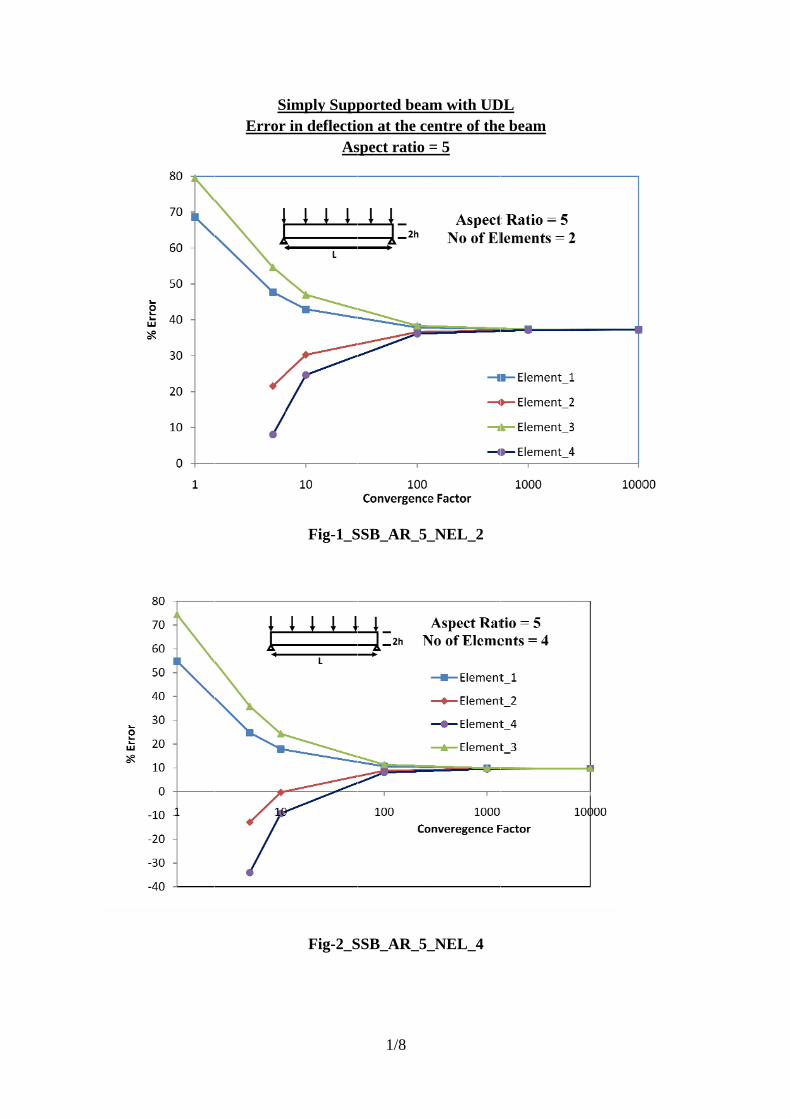
SError
imply Suppin deflectio
As
Fig-1_S
Fig-2_S
1/8
ported beaon at the cespect ratio
SSB_AR_5_
SSB_AR_5_
m with UDentre of the= 5
_NEL_2
_NEL_4
DL e beam
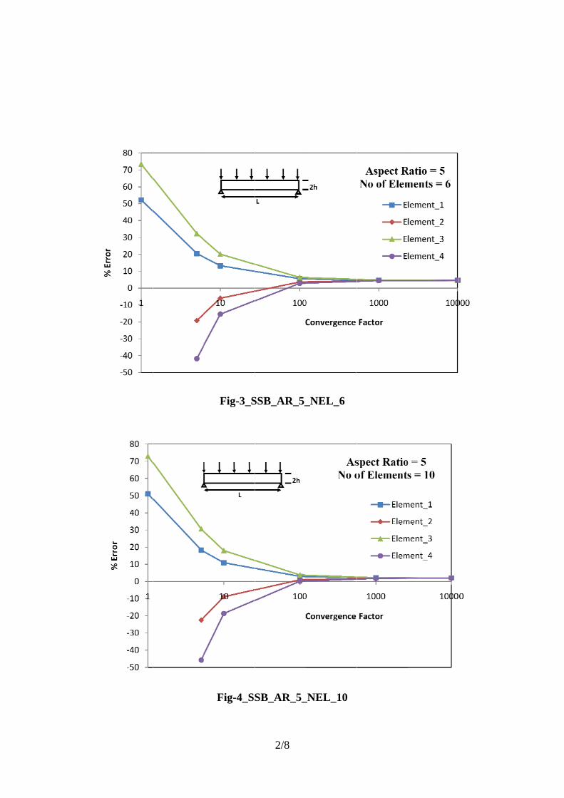
Fig-3_S
Fig-4_SS
2/8
SSB_AR_5_
SB_AR_5_
_NEL_6
_NEL_10
SError
imply Suppin deflectio
Asp
Fig-1_SS
Fig-2_SS
3/8
ported beaon at the cepect ratio =
SB_AR_10
SB_AR_10
m with UDentre of the= 10
0_NEL_2
0_NEL_4
DL e beam
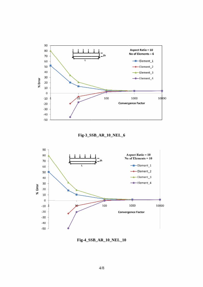
Fig-3_SS
Fig-4_SS
4/8
SB_AR_10
SB_AR_10_
0_NEL_6
_NEL_10
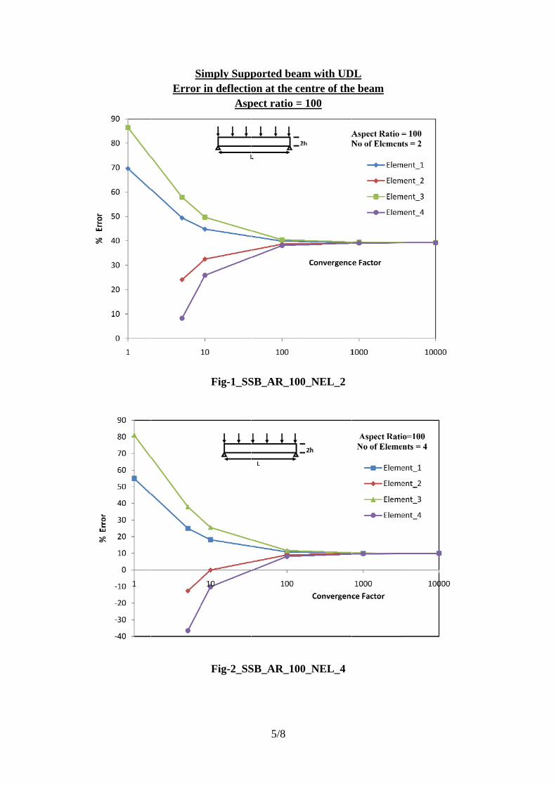
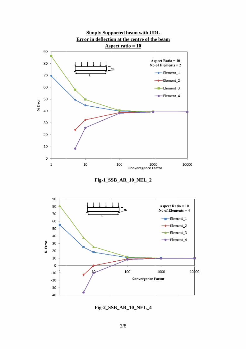
SError
imply Suppin deflectio
Asp
Fig-1_SS
Fig-2_SS
5/8
ported beaon at the ce
pect ratio =
SB_AR_100
SB_AR_100
m with UDentre of the
= 100
0_NEL_2
0_NEL_4
DL e beam
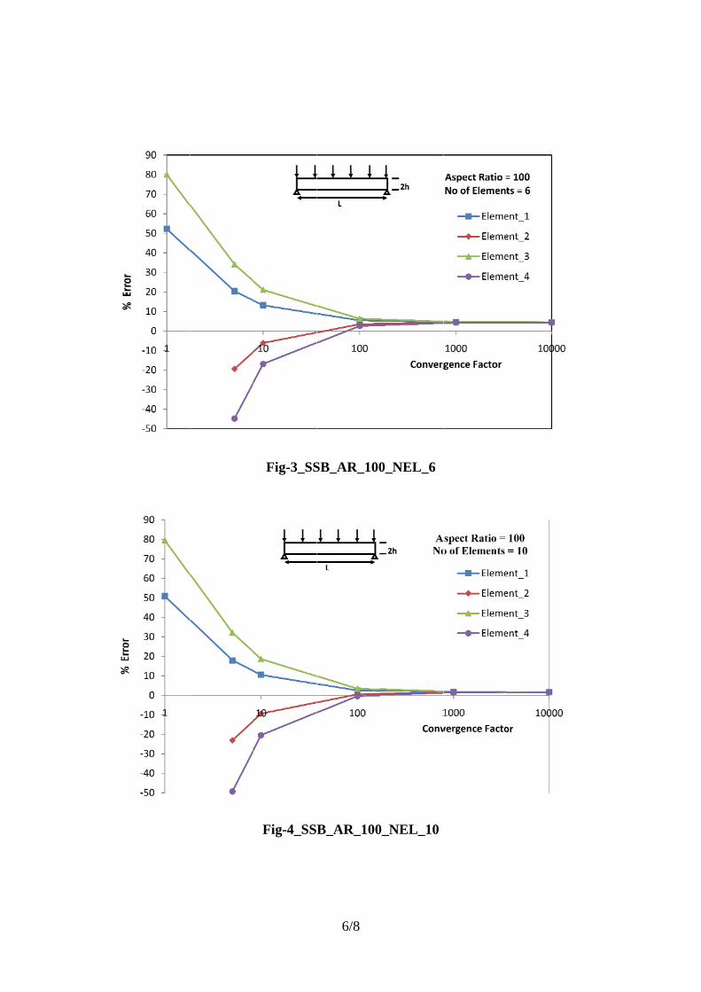
Fig-3_SS
Fig-4_SS
6/8
SB_AR_100
B_AR_100
0_NEL_6
0_NEL_10
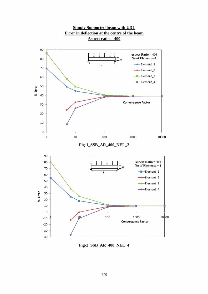
SError
imply Suppin deflectio
Asp
Fig-1_SS
Fig-2_SS
7/8
ported beaon at the ce
pect ratio =
SB_AR_400
SB_AR_400
m with UDentre of the
= 400
0_NEL_2
0_NEL_4
DL e beam
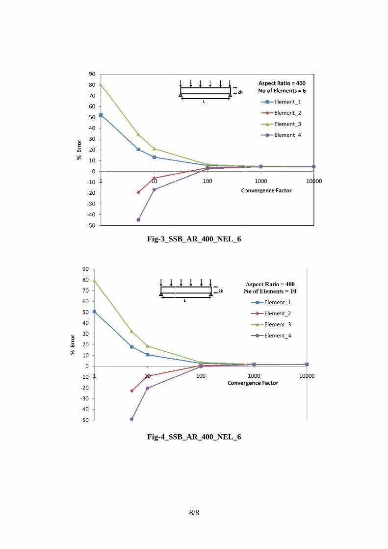
Fig-3_SS
Fig-4_SS
8/8
SB_AR_400
SB_AR_400
0_NEL_6
0_NEL_6
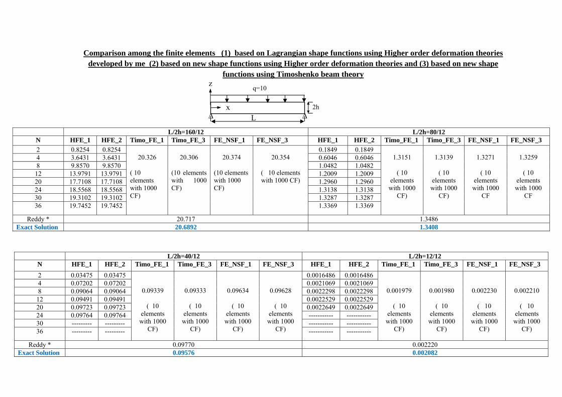
Comparison among the finite elements (1) based on Lagrangian shape functions using Higher order deformation theories developed by me (2) based on new shape functions using Higher order deformation theories and (3) based on new shape
functions using Timoshenko beam theory
L/2h=160/12 L/2h=80/12 N HFE_1 HFE_2 Timo_FE_1 Timo_FE_3 FE_NSF_1 FE_NSF_3 HFE_1 HFE_2 Timo_FE_1 Timo_FE_3 FE_NSF_1 FE_NSF_3
2 0.8254 0.8254 20.326
( 10 elements with 1000 CF)
20.306
(10 elements with 1000 CF)
20.374
(10 elements with 1000 CF)
20.354
( 10 elements with 1000 CF)
0.1849 0.1849 1.3151
( 10
elements with 1000
CF)
1.3139
( 10
elements with 1000
CF)
1.3271
( 10
elements with 1000
CF
1.3259
( 10
elements with 1000
CF
4 3.6431 3.6431 0.6046 0.6046 8 9.8570 9.8570 1.0482 1.0482
12 13.9791 13.9791 1.2009 1.2009 20 17.7108 17.7108 1.2960 1.2960 24 18.5568 18.5568 1.3138 1.3138 30 19.3102 19.3102 1.3287 1.3287 36 19.7452 19.7452 1.3369 1.3369
Reddy * 20.717 1.3486 Exact Solution 20.6892 1.3408
L/2h=40/12 L/2h=12/12 N HFE_1 HFE_2 Timo_FE_1 Timo_FE_3 FE_NSF_1 FE_NSF_3 HFE_1 HFE_2 Timo_FE_1 Timo_FE_3 FE_NSF_1 FE_NSF_3
2 0.03475 0.03475
0.09339
( 10 elements with 1000
CF)
0.09333
( 10 elements with 1000
CF)
0.09634
( 10 elements with 1000
CF)
0.09628
( 10 elements with 1000
CF)
0.0016486 0.0016486
0.001979
( 10 elements with 1000
CF)
0.001980
( 10 elements with 1000
CF)
0.002230
( 10 elements with 1000
CF)
0.002210
( 10 elements with 1000
CF)
4 0.07202 0.07202 0.0021069 0.0021069 8 0.09064 0.09064 0.0022298 0.0022298
12 0.09491 0.09491 0.0022529 0.0022529 20 0.09723 0.09723 0.0022649 0.0022649 24 0.09764 0.09764 ----------- ----------- 30 --------- --------- ----------- ----------- 36 --------- --------- ----------- -----------
Reddy * 0.09770 0.002220 Exact Solution 0.09576 0.002082
q=10
2h
L x
z
ΔΔ
-190.0
Length =5.0
00 -11
-0.50
-0.40
-0.30
-0.20
-0.10
0.00
0.10
0.20
0.30
0.40
0.50
Thic
knes
s
Stres
∆
0, width=1.0, t
14.00
0
0
0
0
0
0
0
0
0
0
0
0.00 5.
2h
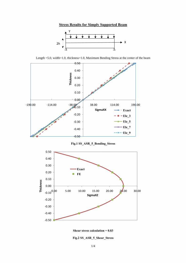
s Results fo
thickness=1.0
Fig.1 SS_A
Shear str
Fig.2 SS_
-0.50
-0.40
-0.30
-0.20
-0.10
0.00
0.10
0.20
0.30
0.40
0.50
-38.00
Thic
knes
s
.00 10.00
ExactFE
Y
1/4
or Simply S
0, Maximum B
ASR_5_Bend
ress calculati
_ASR_5_She
38.00
Sigm
0 15.00SigmaXZ
t
Supported
∆
Bending Stress
ding_Stress
ion = 0.83
ear_Stress
114.00
maXX
20.00
Beam
s at the center
0 190
Exact
Ele_3
Ele_5
Ele_7
Ele_9
25.00 3
X
r of the beam
0.00
30.00
-7800.00 -52
-0.50
-0.40
-0.30
-0.20
-0.10
0.00
0.10
0.20
0.30
0.40
0.50
0Thic
knes
s
Maxi
20.00 -2
0.00 10.
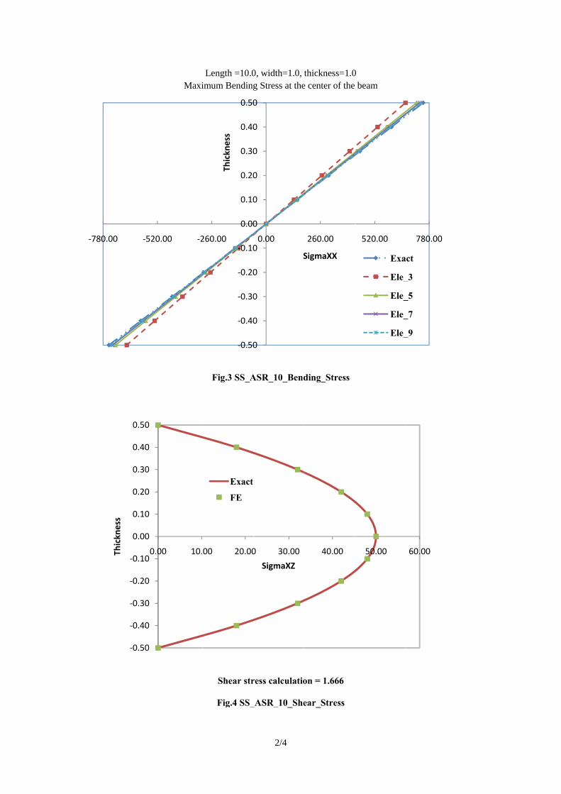
Length =10.0imum Bending
Fig.3 SS_A
Shear str
Fig.4 SS_
-0.50
-0.40
-0.30
-0.20
-0.10
0.00
0.10
0.20
0.30
0.40
0.50
260.00Th
ickn
ess
00 20.00
Exact
FE
2/4
0, width=1.0, g Stress at the
ASR_10_Bend
ress calculatio
_ASR_10_She
0
0
0
0
0
0
0
0
0
0
0
0.00
S
0 30.00
SigmaXZ
thickness=1.0e center of the
ding_Stress
on = 1.666
ear_Stress
260.00
SigmaXX
40.00
0 beam
520.00
Exa
Ele_
Ele_
Ele_
Ele_
50.00
780.00
act
_3
_5
_7
_9
60.00
-3000002.00
-0.50
-0.40
-0.30
-0.20
-0.10
0.00
0.10
0.20
0.30
0.40
0.50
0Thic
knes
s
Maxi
-150001.0
0.00 200
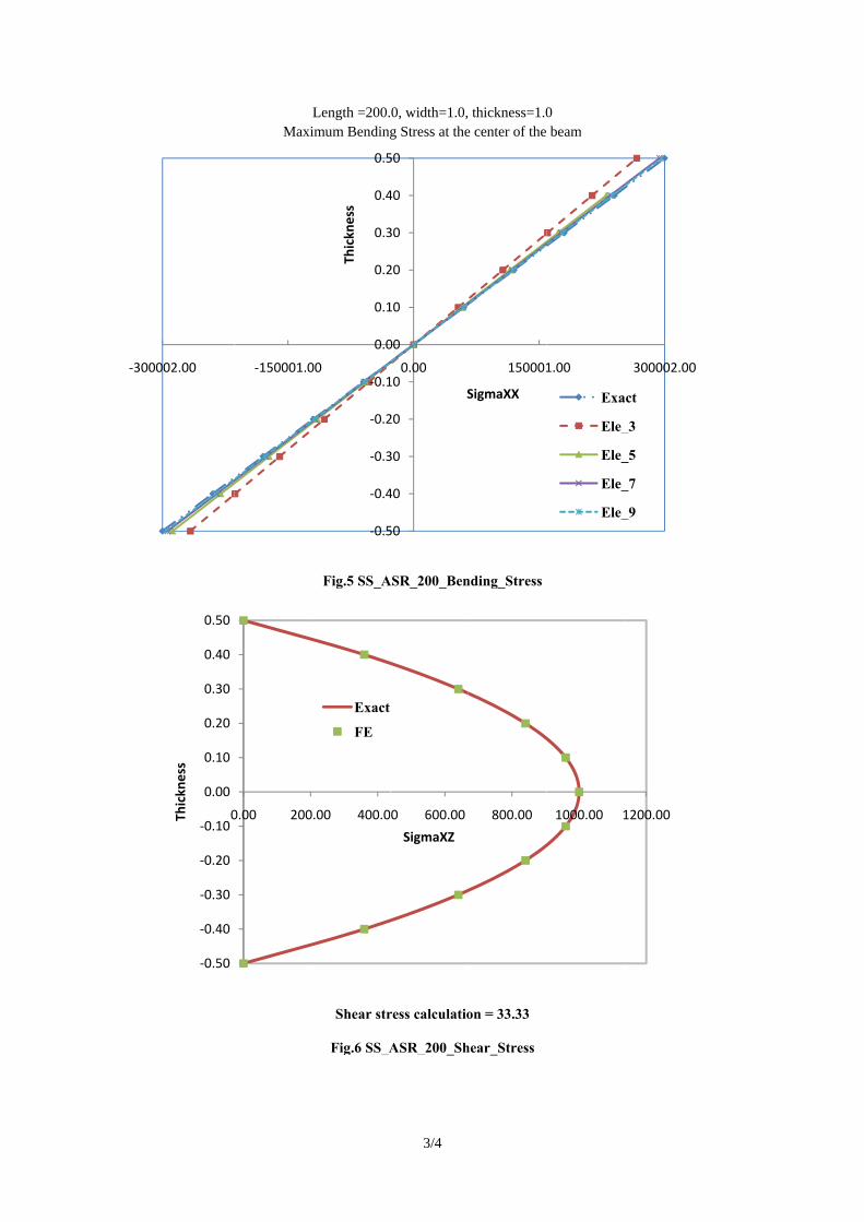
Length =200.imum Bending
Fig.5 SS_A
Shear str
Fig.6 SS_A
-0.5
-0.4
-0.3
-0.2
-0.1
0.0
0.1
0.2
0.3
0.4
0.5
00Th
ickn
ess
.00 400.0
Exact
FE
3/4
0, width=1.0,g Stress at the
ASR_200_Ben
ress calculatio
ASR_200_Sh
50
40
30
20
10
00
10
20
30
40
50
0.00
S
0 600.00
SigmaXZ
thickness=1.0e center of the
nding_Stress
on = 33.33
hear_Stress
150001
SigmaXX
800.00
0 beam
1.00
Exa
Ele_
Ele_
Ele_
Ele_
1000.00 1
300002.00
act
_3
_5
_7
_9
1200.00
-1.5000E+06 -1.0
-0.50
-0.40
-0.30
-0.20
-0.10
0.00
0.10
0.20
0.30
0.40
0.50
0Thic
knes
s
Maxi
000E+06 -5.
0.00 50
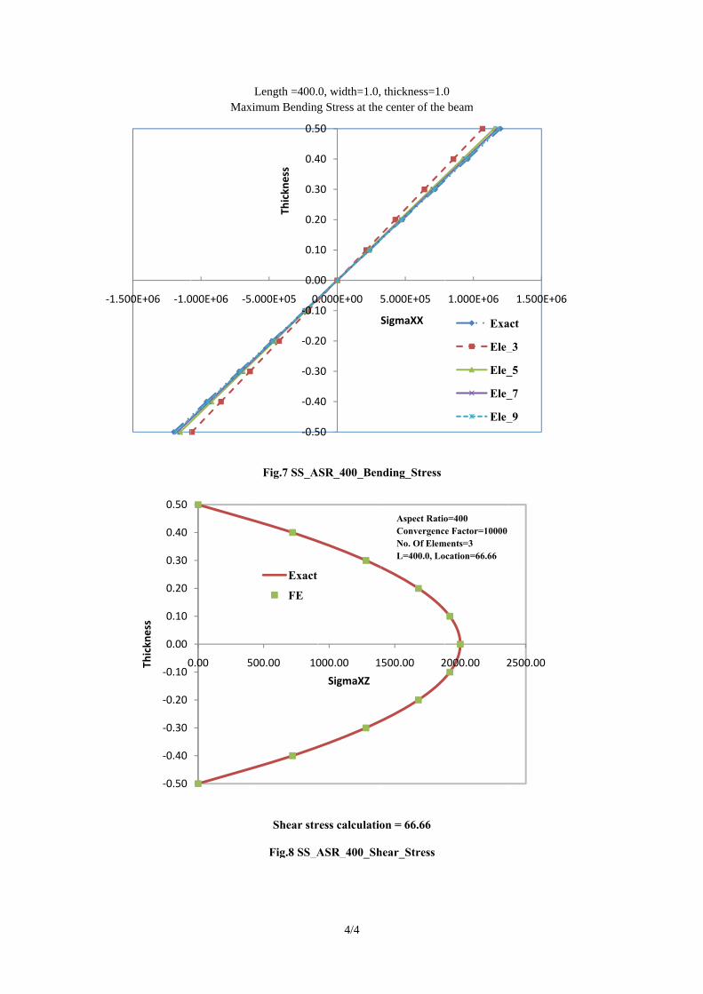
Length =400.imum Bending
Fig.7 SS_A
Shear str
Fig.8 SS_A
-0.5
-0.4
-0.3
-0.2
-0.1
0.0
0.1
0.2
0.3
0.4
0.5
000E+05 0Th
ickn
ess
00.00 10
Exact
FE
4/4
0, width=1.0,g Stress at the
ASR_400_Ben
ress calculatio
ASR_400_Sh
50
40
30
20
10
00
10
20
30
40
50
.000E+00 5
S
000.00 1
SigmaXZ
thickness=1.0e center of the
nding_Stress
on = 66.66
hear_Stress
5.000E+05
SigmaXX
500.00 2
Aspect RatioConvergencNo. Of ElemL=400.0, Lo
0 beam
1.000E+06
Exa
Ele_
Ele_
Ele_
Ele_
2000.00 2
o=400 e Factor=10000
ments=3 ocation=66.66
1.500E+06
act
_3
_5
_7
_9
2500.00
1/8
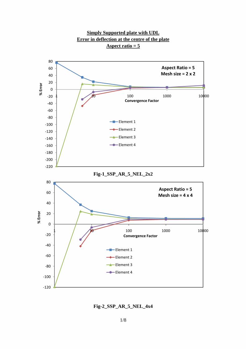
Simply Supported plate with UDL Error in deflection at the centre of the plate
Aspect ratio = 5
Fig-1_SSP_AR_5_NEL_2x2
Fig-2_SSP_AR_5_NEL_4x4
-220
-200
-180
-160
-140
-120
-100
-80
-60
-40
-20
0
20
40
60
80
1 10 100 1000 10000% E
rror
Convergence Factor
Aspect Ratio = 5Mesh size = 2 x 2
Element 1
Element 2
Element 3
Element 4
-120
-100
-80
-60
-40
-20
0
20
40
60
80
1 10 100 1000 10000
% E
rror
Convergence Factor
Aspect Ratio = 5Mesh size = 4 x 4
Element 1
Element 2
Element 3
Element 4
2/8
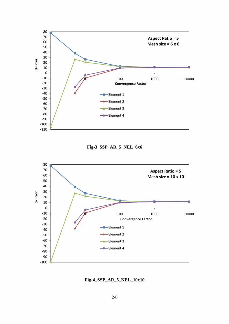
Fig-3_SSP_AR_5_NEL_6x6
Fig-4_SSP_AR_5_NEL_10x10
-110-100
-90-80-70-60-50-40-30-20-10
01020304050607080
1 10 100 1000 10000
% E
rror
Convergence Factor
Aspect Ratio = 5Mesh size = 6 x 6
Element 1
Element 2
Element 3
Element 4
-100-90-80-70-60-50-40-30-20-10
01020304050607080
1 10 100 1000 10000
% E
rror
Convergence Factor
Aspect Ratio = 5Mesh size = 10 x 10
Element 1
Element 2
Element 3
Element 4
3/8
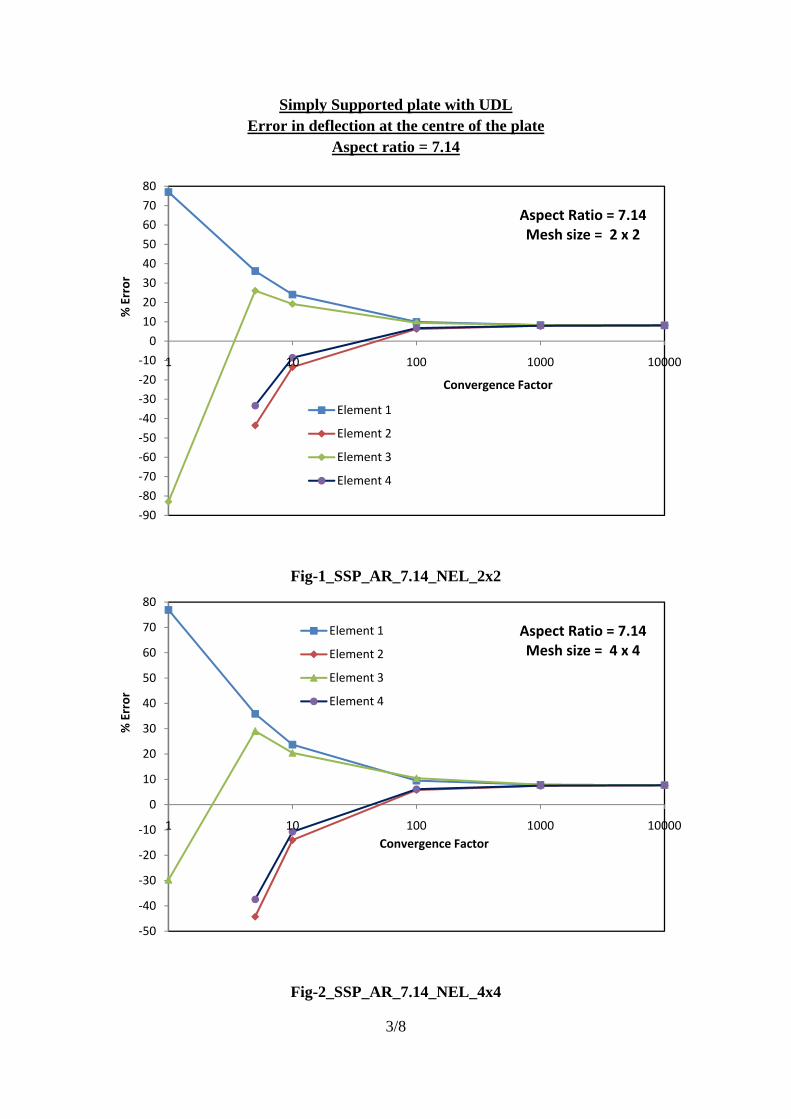
Simply Supported plate with UDL Error in deflection at the centre of the plate
Aspect ratio = 7.14
Fig-1_SSP_AR_7.14_NEL_2x2
Fig-2_SSP_AR_7.14_NEL_4x4
-90
-80
-70
-60
-50
-40
-30
-20
-10
0
10
20
30
40
50
60
70
80
1 10 100 1000 10000
% E
rror
Convergence Factor
Aspect Ratio = 7.14Mesh size = 2 x 2
Element 1
Element 2
Element 3
Element 4
-50
-40
-30
-20
-10
0
10
20
30
40
50
60
70
80
1 10 100 1000 10000
% E
rror
Convergence Factor
Aspect Ratio = 7.14Mesh size = 4 x 4
Element 1
Element 2
Element 3
Element 4

4/8
Fig-3_SSP_AR_7.14_NEL_6x6
Fig-4_SSP_AR_7.14_NEL_10x10
-50
-30
-10
10
30
50
70
1 10 100 1000 10000
% E
rror
Convergence Factor
Aspect Ratio = 7.14Mesh size = 6 x 6
Element 1
Element 2
Element 3
Element 4
-50
-40
-30
-20
-10
0
10
20
30
40
50
60
70
80
1 10 100 1000 10000
% E
rror
Convergence Factor
Aspect Ratio = 7.14Mesh size = 10 x 10
Element 1
Element 2
Element 3
Element 4
5/8
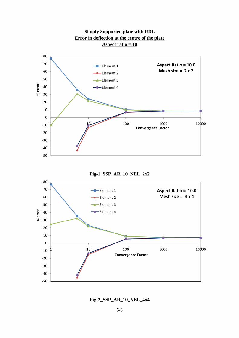
Simply Supported plate with UDL Error in deflection at the centre of the plate
Aspect ratio = 10
Fig-1_SSP_AR_10_NEL_2x2
Fig-2_SSP_AR_10_NEL_4x4
-50
-40
-30
-20
-10
0
10
20
30
40
50
60
70
80
1 10 100 1000 10000
% E
rror
Convergence Factor
Aspect Ratio = 10.0Mesh size = 2 x 2
Element 1
Element 2
Element 3
Element 4
-50
-40
-30
-20
-10
0
10
20
30
40
50
60
70
80
1 10 100 1000 10000
% E
rror
Convergence Factor
Aspect Ratio = 10.0Mesh size = 4 x 4
Element 1
Element 2
Element 3
Element 4
6/8
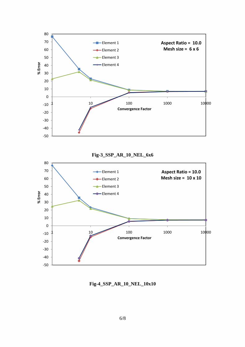
Fig-3_SSP_AR_10_NEL_6x6
Fig-4_SSP_AR_10_NEL_10x10
-50
-40
-30
-20
-10
0
10
20
30
40
50
60
70
80
1 10 100 1000 10000
% E
rror
Convergence Factor
Aspect Ratio = 10.0Mesh size = 6 x 6
Element 1
Element 2
Element 3
Element 4
-50
-40
-30
-20
-10
0
10
20
30
40
50
60
70
80
1 10 100 1000 10000
% E
rror
Convergence Factor
Aspect Ratio = 10.0Mesh size = 10 x 10
Element 1
Element 2
Element 3
Element 4
7/8
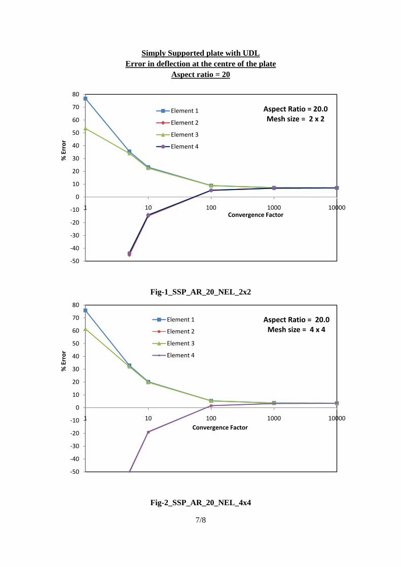
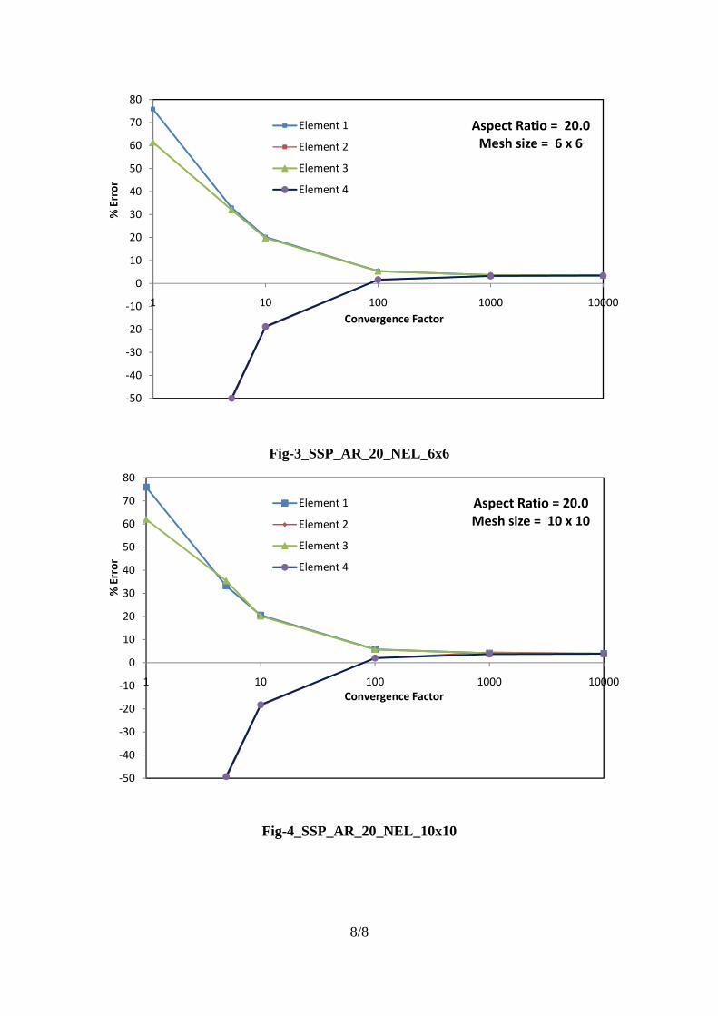
Simply Supported plate with UDL Error in deflection at the centre of the plate
Aspect ratio = 20
Fig-1_SSP_AR_20_NEL_2x2
Fig-2_SSP_AR_20_NEL_4x4
-50
-40
-30
-20
-10
0
10
20
30
40
50
60
70
80
1 10 100 1000 10000
% E
rror
Convergence Factor
Aspect Ratio = 20.0Mesh size = 2 x 2
Element 1
Element 2
Element 3
Element 4
-50
-40
-30
-20
-10
0
10
20
30
40
50
60
70
80
1 10 100 1000 10000
% E
rror
Convergence Factor
Aspect Ratio = 20.0Mesh size = 4 x 4
Element 1
Element 2
Element 3
Element 4
8/8
Fig-3_SSP_AR_20_NEL_6x6
Fig-4_SSP_AR_20_NEL_10x10
-50
-40
-30
-20
-10
0
10
20
30
40
50
60
70
80
1 10 100 1000 10000
% E
rror
Convergence Factor
Aspect Ratio = 20.0Mesh size = 6 x 6
Element 1
Element 2
Element 3
Element 4
-50
-40
-30
-20
-10
0
10
20
30
40
50
60
70
80
1 10 100 1000 10000
% E
rror
Convergence Factor
Aspect Ratio = 20.0Mesh size = 10 x 10
Element 1
Element 2
Element 3
Element 4
12”
12”
1 2
3
4 6 5
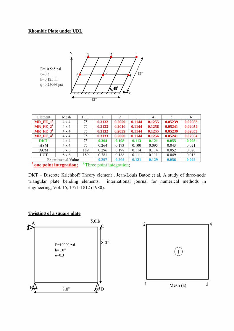
Rhombic Plate under UDL
Element Mesh DOF 1 2 3 4 5 6 MR_FE_11 4 x 4 75 0.3132 0.2059 0.1144 0.1255 0.05239 0.02053 MR_FE_21 4 x 4 75 0.3133 0.2010 0.1144 0.1256 0.05241 0.02054 MR_FE_31 4 x 4 75 0.3132 0.2059 0.1144 0.1255 0.05239 0.02053 MR_FE_41 4 x 4 75 0.3133 0.2060 0.1144 0.1256 0.05241 0.02054
DKT2 4 x 4 75 0.304 0.198 0.113 0.121 0.055 0.028 HSM 4 x 4 75 0.264 0.173 0.100 0.095 0.043 0.021 ACM 8 x 6 189 0.296 0.198 0.114 0.114 0.052 0.020 HCT 8 x 6 189 0.281 0.188 0.111 0.111 0.049 0.018
Experimental Value 0.297 0.204 0.121 0.129 0.056 0.022 1 one point integration; 2 Three point integration;
DKT – Discrete Krichhoff Theory element , Jean-Louis Batoz et al, A study of three-node triangular plate bending elements, international journal for numerical methods in engineering, Vol. 15, 1771-1812 (1980).
Twisting of a square plate
y
x450
E=10.5e5 psi υ=0.3 h=0.125 in q=0.25066 psi
5 · · ·
· · ·
2 C5.0lb
8.0”
8.0”
B
A
D
E=10000 psi h=1.0” υ=0.3
1
4
1 3 Mesh (a)
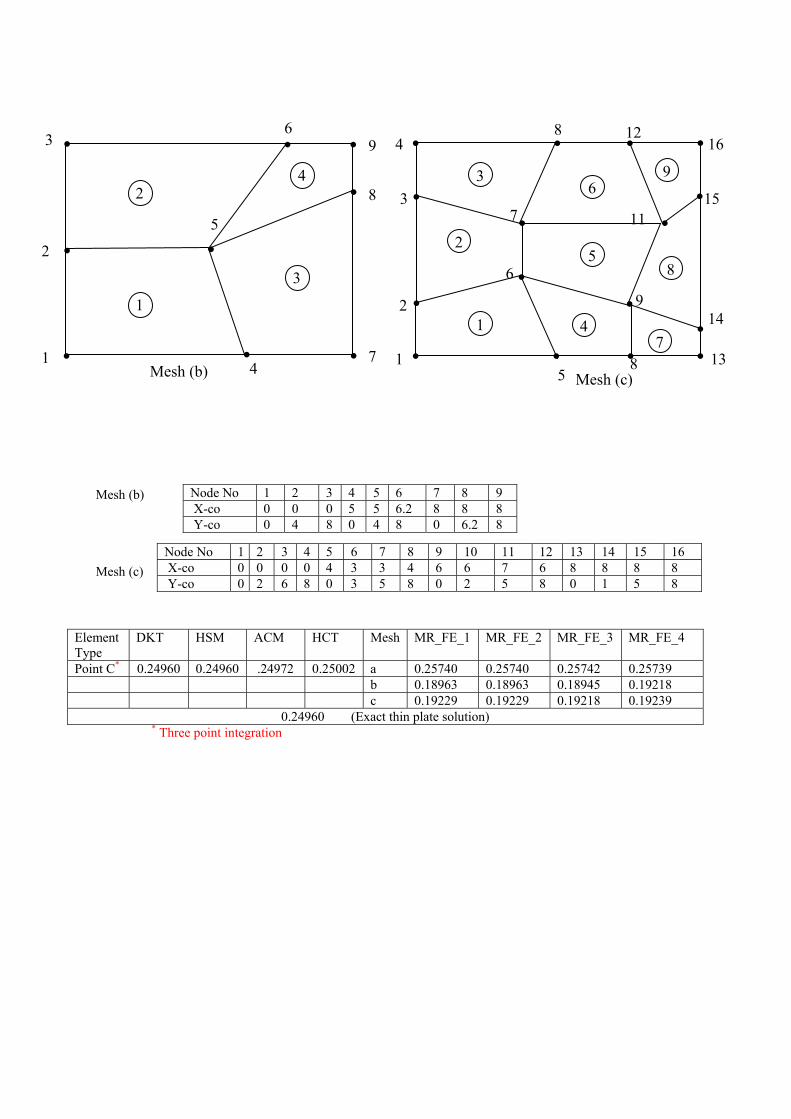
Mesh (b)
Mesh (c)
Element Type
DKT HSM ACM HCT Mesh MR_FE_1 MR_FE_2 MR_FE_3 MR_FE_4
Point C* 0.24960 0.24960 .24972 0.25002 a 0.25740 0.25740 0.25742 0.25739 b 0.18963 0.18963 0.18945 0.19218 c 0.19229 0.19229 0.19218 0.19239
0.24960 (Exact thin plate solution) * Three point integration
Node No 1 2 3 4 5 6 7 8 9 X-co 0 0 0 5 5 6.2 8 8 8 Y-co 0 4 8 0 4 8 0 6.2 8
Node No 1 2 3 4 5 6 7 8 9 10 11 12 13 14 15 16 X-co 0 0 0 0 4 3 3 4 6 6 7 6 8 8 8 8 Y-co 0 2 6 8 0 3 5 8 0 2 5 8 0 1 5 8
6
4 7
9
8
5
3
1
2
4
3
2
1
·
·
·
·
· ·
·
··
Mesh (b)
·
·
· ·
· ·
·
· ·
· · ·
· · · ·
1
2
3
4
7
8
13
12
11
9
8
6
5
14
15
16
1
2
3
4
5
6
7
8
9
Mesh (c)
1/19
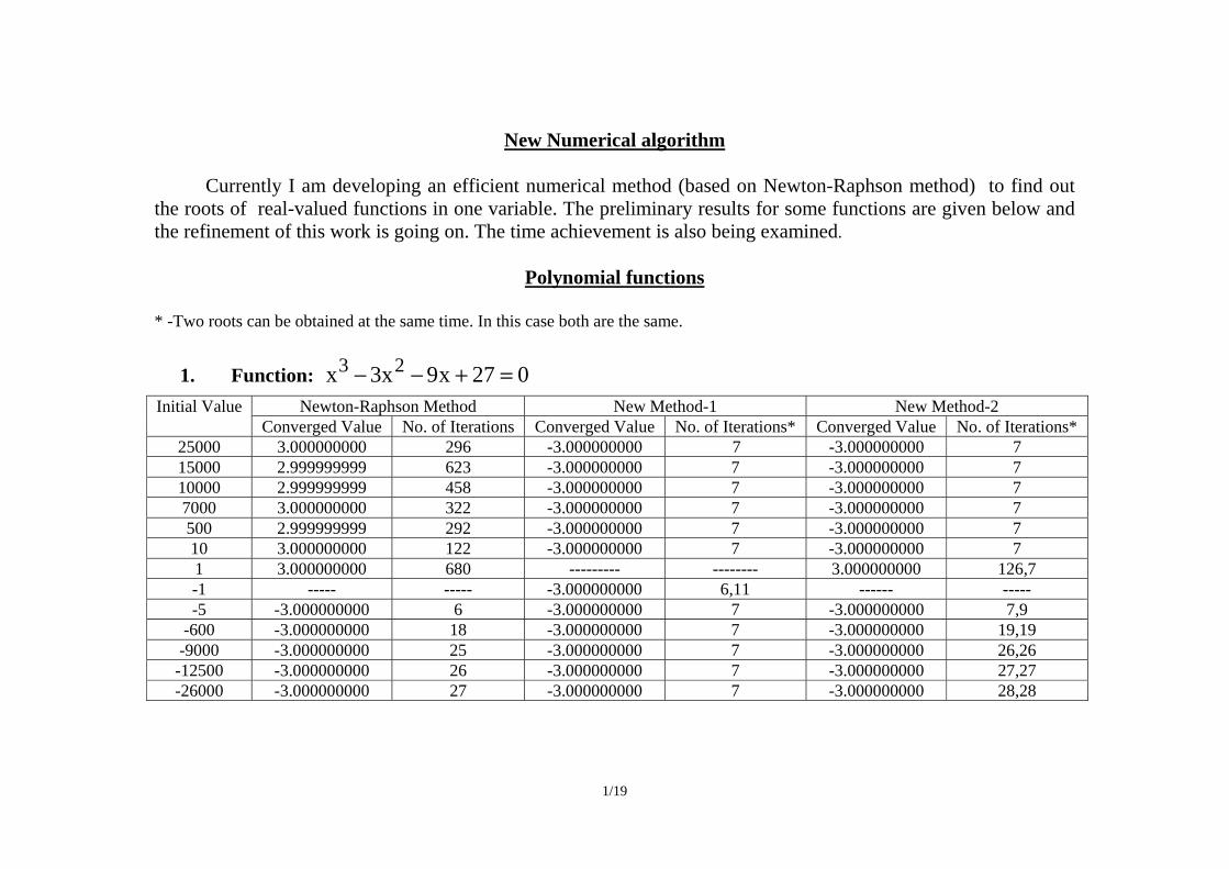
New Numerical algorithm
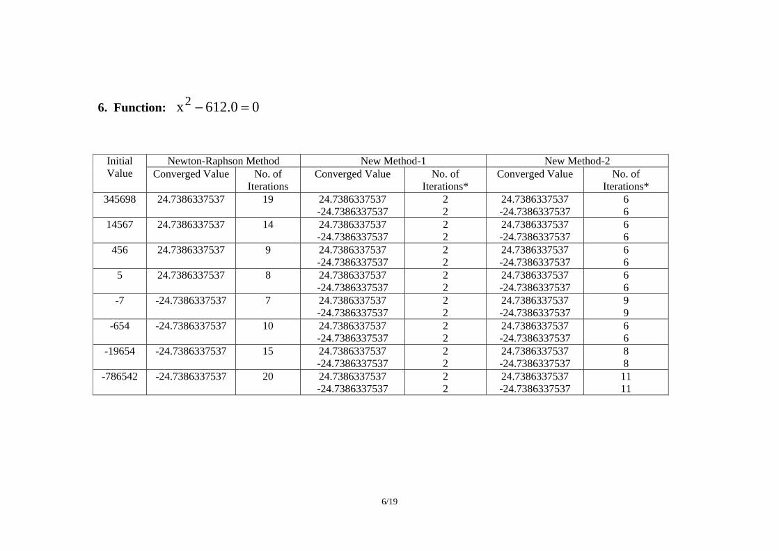
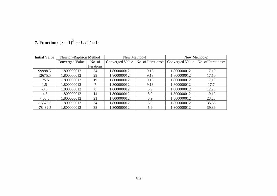
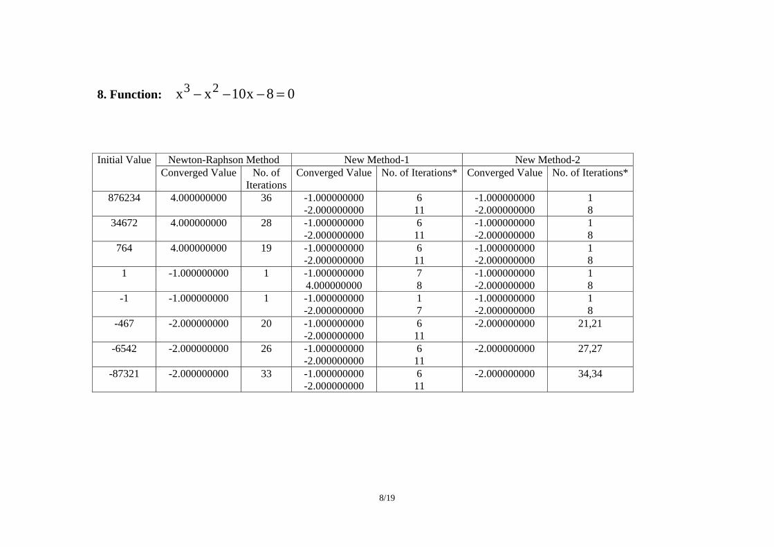
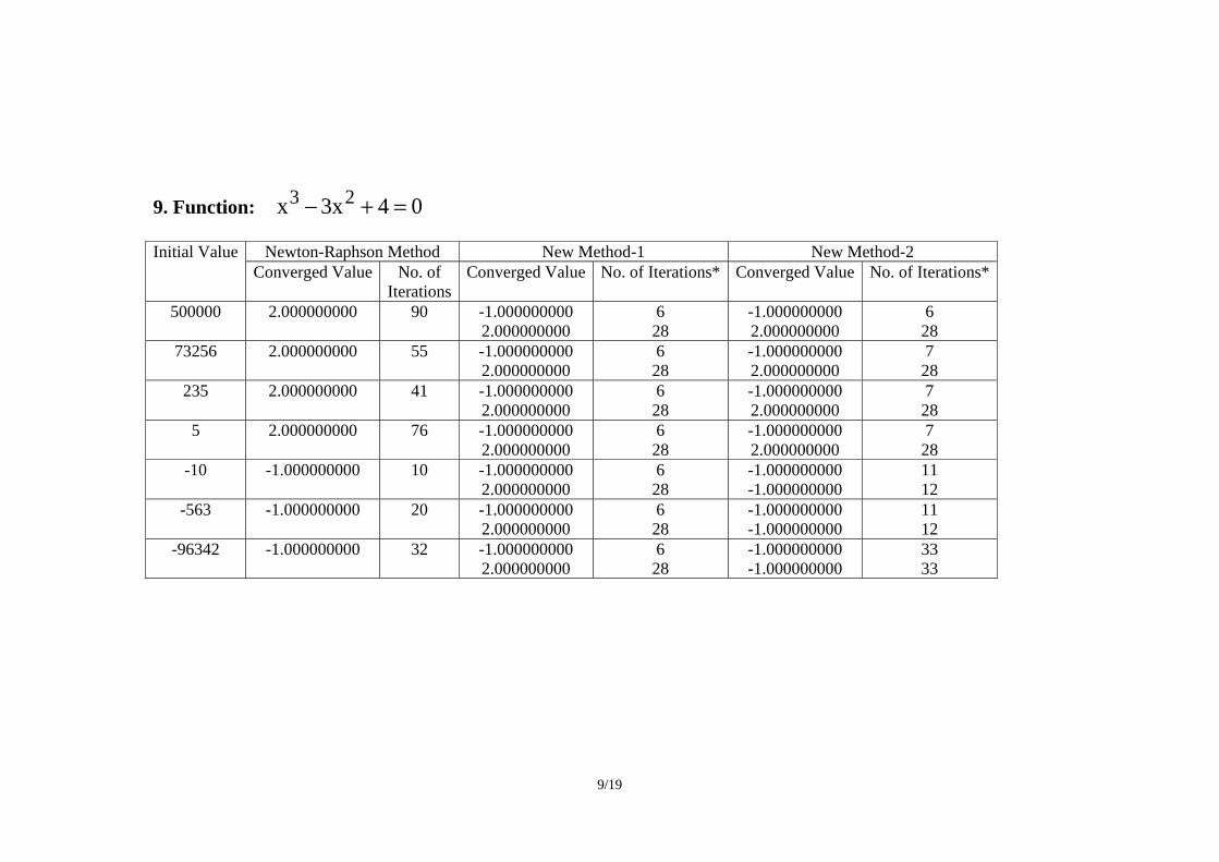
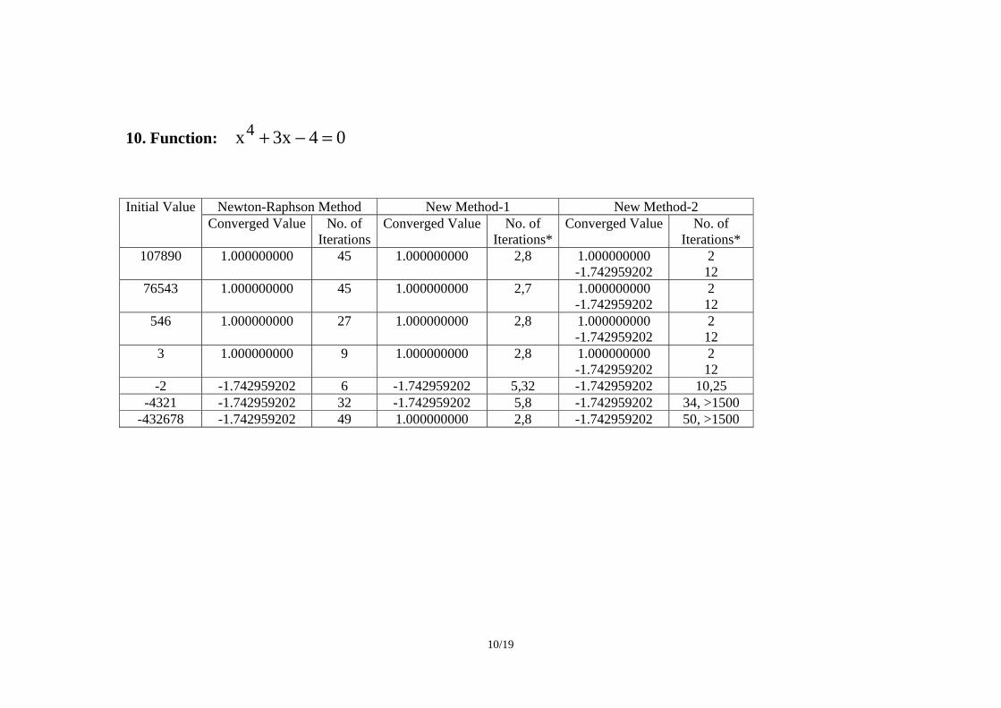
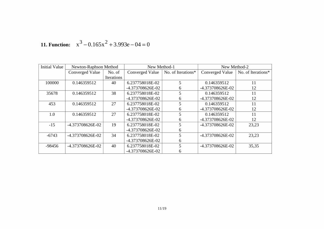
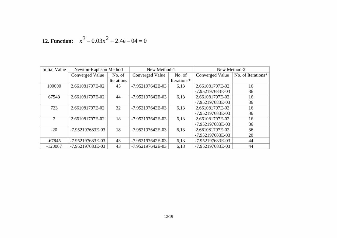
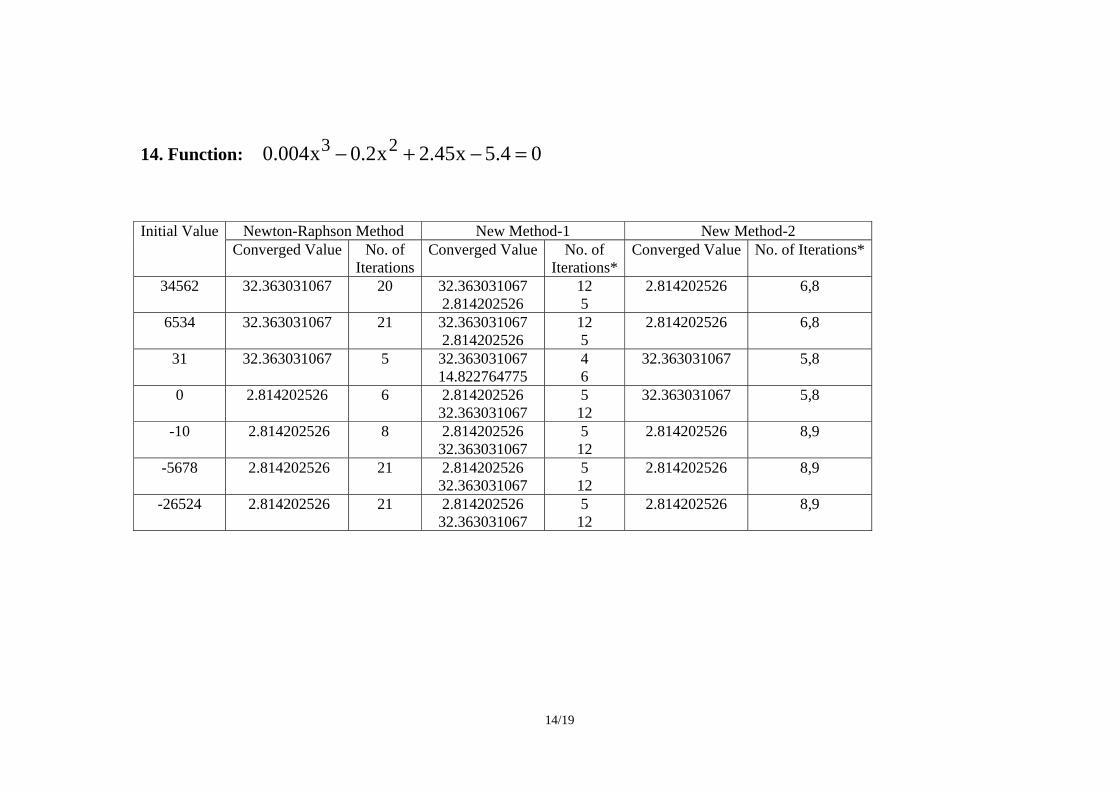
Currently I am developing an efficient numerical method (based on Newton-Raphson method) to find out the roots of real-valued functions in one variable. The preliminary results for some functions are given below and the refinement of this work is going on. The time achievement is also being examined.
Polynomial functions
* -Two roots can be obtained at the same time. In this case both are the same.
1. Function: 027x9x3x 23 =+−−
Initial Value Newton-Raphson Method New Method-1 New Method-2 Converged Value No. of Iterations Converged Value No. of Iterations* Converged Value No. of Iterations*
25000 3.000000000 296 -3.000000000 7 -3.000000000 7 15000 2.999999999 623 -3.000000000 7 -3.000000000 7 10000 2.999999999 458 -3.000000000 7 -3.000000000 7 7000 3.000000000 322 -3.000000000 7 -3.000000000 7 500 2.999999999 292 -3.000000000 7 -3.000000000 7 10 3.000000000 122 -3.000000000 7 -3.000000000 7 1 3.000000000 680 --------- -------- 3.000000000 126,7 -1 ----- ----- -3.000000000 6,11 ------ ----- -5 -3.000000000 6 -3.000000000 7 -3.000000000 7,9
-600 -3.000000000 18 -3.000000000 7 -3.000000000 19,19 -9000 -3.000000000 25 -3.000000000 7 -3.000000000 26,26
-12500 -3.000000000 26 -3.000000000 7 -3.000000000 27,27 -26000 -3.000000000 27 -3.000000000 7 -3.000000000 28,28
2/19
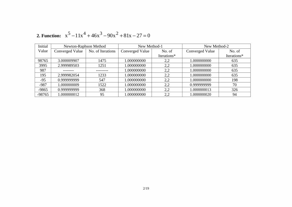
2. Function: 027x81x90x46x11x 2345 =−+−+−
Initial Value
Newton-Raphson Method New Method-1 New Method-2 Converged Value No. of Iterations Converged Value No. of
Iterations* Converged Value No. of
Iterations* 98765 3.000009907 1475 1.000000000 2,2 1.000000000 635 3995 2.999989503 1251 1.000000000 2,2 1.000000000 635 987 -------- --------- 1.000000000 2,2 1.000000000 635 195 2.999982054 1233 1.000000000 2,2 1.000000000 635 -95 0.999999999 547 1.000000000 2,2 1.000000000 198 -987 1.000000009 1522 1.000000000 2,2 0.999999999 70
-9865 0.999999999 368 1.000000000 2,2 1.000000013 326 -98765 1.000000012 95 1.000000000 2,2 1.000000020 94
3/19
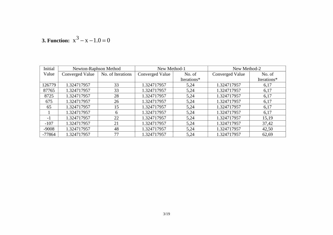
3. Function: 00.1xx3 =−−
Initial Value
Newton-Raphson Method New Method-1 New Method-2 Converged Value No. of Iterations Converged Value No. of
Iterations* Converged Value No. of
Iterations* 126779 1.324717957 33 1.324717957 5,24 1.324717957 6,17 87765 1.324717957 33 1.324717957 5,24 1.324717957 6,17 8725 1.324717957 28 1.324717957 5,24 1.324717957 6,17 675 1.324717957 26 1.324717957 5,24 1.324717957 6,17 65 1.324717957 15 1.324717957 5,24 1.324717957 6,17 1 1.324717957 6 1.324717957 5,24 1.324717957 6,17 -1 1.324717957 22 1.324717957 5,24 1.324717957 15,19
-107 1.324717957 21 1.324717957 5,24 1.324717957 37,42 -9008 1.324717957 48 1.324717957 5,24 1.324717957 42,50
-77864 1.324717957 77 1.324717957 5,24 1.324717957 62,69
4/19
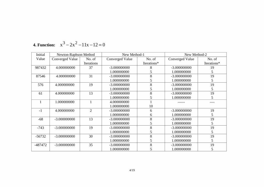
4. Function: 012x11x2x 23 =−−−
Initial Value
Newton-Raphson Method New Method-1 New Method-2 Converged Value No. of
Iterations Converged Value No. of
Iterations* Converged Value No. of
Iterations* 987432 4.000000000 37 -3.000000000
1.000000000 8 5
-3.000000000 1.000000000
19 5
87546 4.000000000 31 -3.000000000 1.000000000
8 5
-3.000000000 1.000000000
19 5
576 4.000000000 19 -3.000000000 1.000000000
8 5
-3.000000000 1.000000000
19 5
61 4.000000000 13 -3.000000000 1.000000000
8 5
-3.000000000 1.000000000
19 5
1 1.000000000 1 4.000000000 1.000000000
1 10
------ ----
-1 4.000000000 2 -3.000000000 1.000000000
6 6
-3.000000000 1.000000000
19 5
-68 -3.000000000 13 -3.000000000 1.000000000
8 5
-3.000000000 1.000000000
19 5
-743 -3.000000000 19 -3.000000000 1.000000000
8 5
-3.000000000 1.000000000
19 5
-56732 -3.000000000 30 -3.000000000 1.000000000
8 5
-3.000000000 1.000000000
19 5
-487472 -3.000000000 35 -3.000000000 1.000000000
8 5
-3.000000000 1.000000000
19 5
5/19
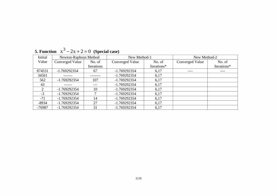
5. Function 02x2x3 =+− (Special case)
Initial Value
Newton-Raphson Method New Method-1 New Method-2 Converged Value No. of
Iterations Converged Value No. of
Iterations* Converged Value No. of
Iterations* 874531 -1.769292354 67 -1.769292354 6,17 ---- ---- 34561 ------- -------- -1.769292354 6,17 562 -1.769292354 107 -1.769292354 6,17 43 ------ --- -1.769292354 6,17 2 -1.769292354 10 -1.769292354 6,17 -3 -1.769292354 7 -1.769292354 6,17 -71 -1.769292354 14 -1.769292354 6,17
-8934 -1.769292354 27 -1.769292354 6,17 -76987 -1.769292354 31 -1.769292354 6,17
6/19
6. Function: 00.612x2 =−
Initial Value
Newton-Raphson Method New Method-1 New Method-2 Converged Value No. of
Iterations Converged Value No. of
Iterations* Converged Value No. of
Iterations* 345698 24.7386337537 19 24.7386337537
-24.7386337537 2 2
24.7386337537 -24.7386337537
6 6
14567 24.7386337537 14 24.7386337537 -24.7386337537
2 2
24.7386337537 -24.7386337537
6 6
456 24.7386337537 9 24.7386337537 -24.7386337537
2 2
24.7386337537 -24.7386337537
6 6
5 24.7386337537 8 24.7386337537 -24.7386337537
2 2
24.7386337537 -24.7386337537
6 6
-7 -24.7386337537 7 24.7386337537 -24.7386337537
2 2
24.7386337537 -24.7386337537
9 9
-654 -24.7386337537 10 24.7386337537 -24.7386337537
2 2
24.7386337537 -24.7386337537
6 6
-19654 -24.7386337537 15 24.7386337537 -24.7386337537
2 2
24.7386337537 -24.7386337537
8 8
-786542 -24.7386337537 20 24.7386337537 -24.7386337537
2 2
24.7386337537 -24.7386337537
11 11
7/19
7. Function: 0512.0)1x( 3 =+−
Initial Value Newton-Raphson Method New Method-1 New Method-2 Converged Value No. of
IterationsConverged Value No. of Iterations* Converged Value No. of Iterations*
99998.5 1.800000012 34 1.800000012 9,13 1.800000012 17,10 12675.5 1.800000012 29 1.800000012 9,13 1.800000012 17,10 175.5 1.800000012 19 1.800000012 9,13 1.800000012 17,10
1.5 1.800000012 7 1.800000012 9,13 1.800000012 17,7 -0.5 1.800000012 8 1.800000012 5,9 1.800000012 12,20 -4.5 1.800000012 14 1.800000012 5,9 1.800000012 19,19
-453.5 1.800000012 21 1.800000012 5,9 1.800000012 23,25 -15673.5 1.800000012 34 1.800000012 5,9 1.800000012 35,35 -78432.5 1.800000012 38 1.800000012 5,9 1.800000012 39,39
8/19
8. Function: 08x10xx 23 =−−−
Initial Value Newton-Raphson Method New Method-1 New Method-2 Converged Value No. of
IterationsConverged Value No. of Iterations* Converged Value No. of Iterations*
876234 4.000000000 36 -1.000000000 -2.000000000
6 11
-1.000000000 -2.000000000
1 8
34672 4.000000000 28 -1.000000000 -2.000000000
6 11
-1.000000000 -2.000000000
1 8
764 4.000000000 19 -1.000000000 -2.000000000
6 11
-1.000000000 -2.000000000
1 8
1 -1.000000000 1 -1.000000000 4.000000000
7 8
-1.000000000 -2.000000000
1 8
-1 -1.000000000 1 -1.000000000 -2.000000000
1 7
-1.000000000 -2.000000000
1 8
-467 -2.000000000 20 -1.000000000 -2.000000000
6 11
-2.000000000 21,21
-6542 -2.000000000 26 -1.000000000 -2.000000000
6 11
-2.000000000 27,27
-87321 -2.000000000 33 -1.000000000 -2.000000000
6 11
-2.000000000 34,34
9/19
9. Function: 04x3x 23 =+−
Initial Value Newton-Raphson Method New Method-1 New Method-2 Converged Value No. of
IterationsConverged Value No. of Iterations* Converged Value No. of Iterations*
500000 2.000000000 90 -1.000000000 2.000000000
6 28
-1.000000000 2.000000000
6 28
73256 2.000000000 55 -1.000000000 2.000000000
6 28
-1.000000000 2.000000000
7 28
235 2.000000000 41 -1.000000000 2.000000000
6 28
-1.000000000 2.000000000
7 28
5 2.000000000 76 -1.000000000 2.000000000
6 28
-1.000000000 2.000000000
7 28
-10 -1.000000000 10 -1.000000000 2.000000000
6 28
-1.000000000 -1.000000000
11 12
-563 -1.000000000 20 -1.000000000 2.000000000
6 28
-1.000000000 -1.000000000
11 12
-96342 -1.000000000 32 -1.000000000 2.000000000
6 28
-1.000000000 -1.000000000
33 33
10/19
10. Function: 04x3x4 =−+
Initial Value Newton-Raphson Method New Method-1 New Method-2 Converged Value No. of
IterationsConverged Value No. of
Iterations* Converged Value No. of
Iterations* 107890 1.000000000 45 1.000000000 2,8 1.000000000
-1.742959202 2
12 76543 1.000000000 45 1.000000000 2,7 1.000000000
-1.742959202 2
12 546 1.000000000 27 1.000000000 2,8 1.000000000
-1.742959202 2
12 3 1.000000000 9 1.000000000 2,8 1.000000000
-1.742959202 2
12 -2 -1.742959202 6 -1.742959202 5,32 -1.742959202 10,25
-4321 -1.742959202 32 -1.742959202 5,8 -1.742959202 34, >1500 -432678 -1.742959202 49 1.000000000 2,8 -1.742959202 50, >1500
11/19
11. Function: 004e993.3x165.0x 23 =−+−
Initial Value Newton-Raphson Method New Method-1 New Method-2 Converged Value No. of
IterationsConverged Value No. of Iterations* Converged Value No. of Iterations*
100000 0.146359512 40 6.237758018E-02 -4.373708626E-02
5 6
0.146359512 -4.373708626E-02
11 12
35678 0.146359512 38 6.237758018E-02 -4.373708626E-02
5 6
0.146359512 -4.373708626E-02
11 12
453 0.146359512 27 6.237758018E-02 -4.373708626E-02
5 6
0.146359512 -4.373708626E-02
11 12
1.0 0.146359512 27 6.237758018E-02 -4.373708626E-02
5 6
0.146359512 -4.373708626E-02
11 12
-15 -4.373708626E-02 19 6.237758018E-02 -4.373708626E-02
5 6
-4.373708626E-02 23,23
-6743 -4.373708626E-02 34 6.237758018E-02 -4.373708626E-02
5 6
-4.373708626E-02 23,23
-98456 -4.373708626E-02 40 6.237758018E-02 -4.373708626E-02
5 6
-4.373708626E-02 35,35
12/19
12. Function: 004e4.2x03.0x 23 =−+−
Initial Value Newton-Raphson Method New Method-1 New Method-2 Converged Value No. of
IterationsConverged Value No. of
Iterations* Converged Value No. of Iterations*
100000 2.661081797E-02 45 -7.952197642E-03
6,13 2.661081797E-02 -7.952197683E-03
16 36
67543 2.661081797E-02 44 -7.952197642E-03 6,13 2.661081797E-02 -7.952197683E-03
16 36
723 2.661081797E-02 32 -7.952197642E-03
6,13 2.661081797E-02 -7.952197683E-03
16 36
2 2.661081797E-02 18 -7.952197642E-03
6,13 2.661081797E-02 -7.952197683E-03
16 36
-20 -7.952197683E-03 18 -7.952197642E-03
6,13 2.661081797E-02 -7.952197683E-03
36 20
-67845 -7.952197683E-03 43 -7.952197642E-03 6,13 -7.952197683E-03 44 -120007 -7.952197683E-03 43 -7.952197642E-03 6,13 -7.952197683E-03 44

13/19
13. Function: 0546.0x21.4x5.3x2 23 =+−+
Initial Value Newton-Raphson Method New Method-1 New Method-2 Converged Value No. of
IterationsConverged Value No. of
Iterations* Converged Value No. of
Iterations*564327 0.700000007 38 0.700000006
0.149999999 8 5
-2.600000005 0.149999999
8 6
5637 0.700000007 28 0.700000006 0.149999999
8 5
-2.600000005 0.149999999
8 6
74 0.700000007 17 0.700000006 0.149999999
8 5
-2.600000005 0.149999999
8 6
0 0.149999999 5 0.700000006 0.149999999
8 5
-2.600000005 0.149999999
8 6
-13 -2.600000005
10 0.700000006 0.149999999
8 5
-2.600000005 0.149999999
8 6
-2451 -2.600000005
23 0.700000006 0.149999999
8 5
-2.600000005
24,25
-123867 -2.600000005
33 0.700000006 0.149999999
8 5
-2.600000005
24,25
14/19
14. Function: 04.5x45.2x2.0x004.0 23 =−+−
Initial Value Newton-Raphson Method New Method-1 New Method-2 Converged Value No. of
IterationsConverged Value No. of
Iterations* Converged Value No. of Iterations*
34562 32.363031067 20 32.363031067 2.814202526
12 5
2.814202526 6,8
6534 32.363031067 21 32.363031067 2.814202526
12 5
2.814202526 6,8
31 32.363031067 5 32.363031067 14.822764775
4 6
32.363031067 5,8
0 2.814202526 6 2.814202526 32.363031067
5 12
32.363031067 5,8
-10 2.814202526 8 2.814202526 32.363031067
5 12
2.814202526
8,9
-5678 2.814202526 21 2.814202526 32.363031067
5 12
2.814202526
8,9
-26524 2.814202526 21 2.814202526 32.363031067
5 12
2.814202526
8,9
15/19
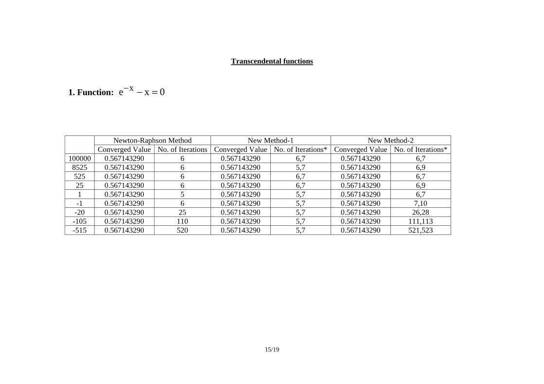
Transcendental functions
1. Function: 0xe x =−−
Newton-Raphson Method New Method-1 New Method-2 Converged Value No. of Iterations Converged Value No. of Iterations* Converged Value No. of Iterations*
100000 0.567143290 6 0.567143290 6,7 0.567143290 6,7 8525 0.567143290 6 0.567143290 5,7 0.567143290 6,9 525 0.567143290 6 0.567143290 6,7 0.567143290 6,7 25 0.567143290 6 0.567143290 6,7 0.567143290 6,9 1 0.567143290 5 0.567143290 5,7 0.567143290 6,7 -1 0.567143290 6 0.567143290 5,7 0.567143290 7,10 -20 0.567143290 25 0.567143290 5,7 0.567143290 26,28
-105 0.567143290 110 0.567143290 5,7 0.567143290 111,113 -515 0.567143290 520 0.567143290 5,7 0.567143290 521,523
16/19
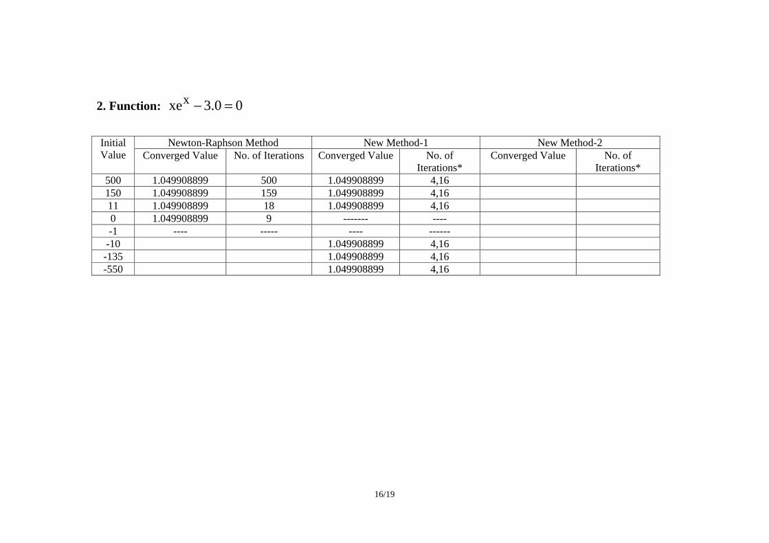
2. Function: 00.3xex =−
Initial Value
Newton-Raphson Method New Method-1 New Method-2 Converged Value No. of Iterations Converged Value No. of
Iterations* Converged Value No. of
Iterations* 500 1.049908899 500 1.049908899 4,16 150 1.049908899 159 1.049908899 4,16 11 1.049908899 18 1.049908899 4,16 0 1.049908899 9 ------- ---- -1 ---- ----- ---- ------
-10 1.049908899 4,16 -135 1.049908899 4,16 -550 1.049908899 4,16
17/19
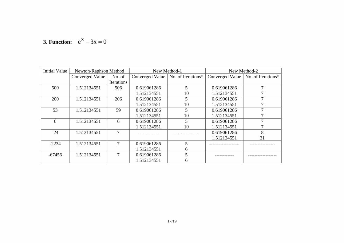
3. Function: 0x3ex =−
Initial Value Newton-Raphson Method New Method-1 New Method-2 Converged Value No. of
IterationsConverged Value No. of Iterations* Converged Value No. of Iterations*
500 1.512134551 506 0.619061286 1.512134551
5 10
0.619061286 1.512134551
7 7
200 1.512134551 206 0.619061286 1.512134551
5 10
0.619061286 1.512134551
7 7
53 1.512134551 59 0.619061286 1.512134551
5 10
0.619061286 1.512134551
7 7
0 1.512134551 6 0.619061286 1.512134551
5 10
0.619061286 1.512134551
7 7
-24 1.512134551 7 ------------ ---------------- 0.619061286 1.512134551
8 31
-2234 1.512134551 7 0.619061286 1.512134551
5 6
------------------- ----------------
-67456 1.512134551 7 0.619061286 1.512134551
5 6
------------ ------------------
18/19
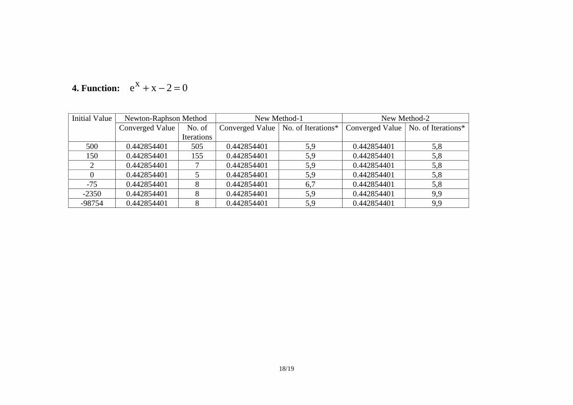
4. Function: 02xex =−+
Initial Value Newton-Raphson Method New Method-1 New Method-2 Converged Value No. of
IterationsConverged Value No. of Iterations* Converged Value No. of Iterations*
500 0.442854401 505 0.442854401 5,9 0.442854401 5,8 150 0.442854401 155 0.442854401 5,9 0.442854401 5,8
2 0.442854401 7 0.442854401 5,9 0.442854401 5,8 0 0.442854401 5 0.442854401 5,9 0.442854401 5,8
-75 0.442854401 8 0.442854401 6,7 0.442854401 5,8 -2350 0.442854401 8 0.442854401 5,9 0.442854401 9,9
-98754 0.442854401 8 0.442854401 5,9 0.442854401 9,9
19/19
Conclusion
1. The first algorithm is independent of initial guess. 2. It converges very faster than the other two, that is, the Newton-Raphson method
and New Method-2.
3. The modifications carried out in the present two algorithms are very simple and the mathematical expressions used are very short statements involving only arithmetic operations.
4. The performance of the first algorithm is far better than that of the other two and
in some cases the performance of the second algorithm is similar to that of the Newton-Raphson method.
5. In some cases, two different roots are simultaneously obtained by these two
algorithms. In the case of the NR method, it is not possible.
Future Work The above work is extended to the analysis of a system of non linear equations in ‘n’ variables to examine the performance of the algorithm.