Embed Size (px)
Citation preview
Numerical prediction of nanoparticle
formation in flames
Dissertation
zur Erlangung des akademischen Grades
Doktoringenieur
(Dr.-Ing.)
von M.Tech. Thirumalesha Chittipotula
geb.am 02 July 1980 in Bhongir, Indien
genehmigt durch die Fakultat fur Verfahrens- und Systemtechnik
der Otto-von-Guericke-Universitat, Magdeburg
Gutachter: Prof. Dr.-Ing. Dominique TheveninProf. Dr.-Ing. Fabian MaußProf. Dr.-Ing. Mirko Peglow
Promotionskolloquium am : 26th Oct. 2012

To my
Mother
Acknowledgement
It gives me immense pleasure to thank everyone who have directly and indirectly
helped and motivated me all through the journey of my PhD. I extend my heartfelt
gratitude to Prof. Dominique Thevenin, an inspiring personality and one of the
best guides I happened to come across. I have learnt much more things by merely
observing him than speaking to him. His outstanding guidance and support in
technical as well as in my career prospects has been extremely helpful.
I convey my sincere thanks to Dr. Gabor Janiga who is easily accessible. His help
in all technical applications including CFD was extremely beneficial, particularly
during initial stages of my work. I extend my sincere thanks to Prof. Peglow,
Prof. Marchisio and Dr. Alper Oncul for the thought-provoking discussions and for
their help on PBE, QMOM and DQMOM. I am thankful to all my fellow doctoral
colleagues both from LSS and IMPRS for all the lively discussions.
I thank the Faculty of Process and Systems Engineering of the Otto-von-Guericke-
Universitat, Magdeburg for providing all the facilities required to carry out my re-
search. My sincere thanks to International Max Planck Research School (IMPRS)
in Magdeburg for financing my doctoral study. The life would not have been so easy
as it is now without Dr. Barbara Witter. I would like to acknowledge her help in
all IMPRS matters and VISA related works.
It always gives me a sense of happiness and responsibility when I recollect all
the support and the contribution of my family members. I am greatly indebted to
my mother Jayamma, brother Sridhar, vadina (Suvarna), sisters (Sumathi, Srivani)
and brothers-in-law (Narsimha, Upender). I am sure that my gratitude shown here
would not be sufficient to equate their warm-hearted embrace all the way of my
journey. I thank God for all the invaluable smiles of wonderful kids in our family.
I am very thankful to Satya Sekhar, Kasyap and Gayathri for proof reading a
few chapters of my thesis. I thank all my friends here in Magdeburg, India and
in the US for their best wishes. Anil, Bablu, Raj Kumar, Kanthu, Sambu, Subbu,
Chitti kanna, Swami Rao, Koti, Suku, Santhosh, Polu, Manju, Raman, Ashok,
Jim, Ganesh, Rayees, Subbru, Yash, Luis, Subba Rayudu, Naresh babu, Dileep and
Rokkam with whom I always enjoyed the company and warmth of their friendship.
Finally, I would like to thank my wife Lakshmi for her love, support and caring
hand.
i

Abstract
Objective of the present study is to accurately model nanoparticle for-
mation in flames and improve existing physico-chemical models involved in
the particulate phase. First and major part of the current study involved
prediction of soot particle formation in turbulent ethylene/air non-premixed
flames. In a second part, synthesis of TiO2 nanoparticles is investigated in
methane/oxygen diffusion flames with titanium tetraisopropoxide (TTIP) as
precursor.
When considering soot formation in practical burners, semi-empirical mod-
els are mostly used. But existing soot models for non-premixed ethylene/air
flames often do not satisfactorily predict soot volume fraction (fv), the key en-
gineering quantity for most applications. Due to intense energy exchange by
radiative heat transfer, this leads to a situation where even basic scalar fields
like temperature are inaccurately described. The objective of the present study
is to develop an enhanced soot prediction model for such flames, valid for a
wide range of flow and operating conditions. The emphasis in this work is
specifically on the particulate phase and not on gas-phase kinetics.
The evolution of soot particles is described by physical models account-
ing for nucleation, surface growth, aggregation and oxidation. The Direct
Quadrature Method of Moments (DQMOM) is employed to solve the Popula-
tion Balance Equations (PBE) in a computationally efficient manner, assuming
a mono-variate PBE with particle diameter as internal coordinate.
The original soot model is optimized numerically by using Genetic Algo-
rithms coupled with Computational Fluid Dynamics (CFD). The values of
three model parameters, associated with nucleation, oxidation and soot parti-
cle radiation are optimized through comparison with recent experimental re-
sults. Two objective functions are formulated based on the difference between
experimental and simulation results for temperature and fv. After obtaining
an optimal parameter set, the resulting model is further tested against three
experimental configurations, leading to a good agreement and thus demon-
strating a high level of generality. Nevertheless, a shift in the peak soot posi-
tion towards the burner was systematically observed at first. This issue could
be finally solved by refining the description of turbulence/chemistry coupling
ii
using a flamelet model and adding another optimization parameter.
Radiative heat transfer is highly significant in combustion processes, es-
pecially for those involving soot. Due to the tight coupling of soot models
with the temperature, it is essential to take into account radiative heat trans-
fer associated with soot particles as well as with key gaseous species while
keeping acceptable numerical complexity. In the present project, three sim-
ple soot radiation models based on grey gas and optically thin approximation
have been analyzed, compared and optimized in an effort to further improve
the particulate models previously developed. The final results are in slightly
better agreement with all measured fields, demonstrating that optimization
based on flow simulations can efficiently support the development of optimal
physico-chemical models.
The second objective of the present numerical analysis is to investigate the
production of TiO2 nanoparticles with tailored mean properties in turbulent
diffusion flames burning CH4 in O2, with titanium tetraisopropoxide (TTIP)
as precursor and argon as carrier gas. Gas-phase chemistry is represented
by considering a detailed CH4-O2 combustion mechanism with 17 species and
41 reactions. The Eddy Dissipation Concept (EDC) model is used to handle
turbulence-chemistry interaction. A Monovariate Population Balance Equa-
tions (PBE) describing the TiO2 nanoparticle evolution is implemented, taking
into account nucleation, molecular growth and aggregation as source terms.
The Quadrature Method of Moments (QMOM) is employed to solve this PBE.
Initially, simulations are performed for 3 different oxygen flow rates (2, 4,
6 L/min) to validate employed models and numerical approach against the ex-
perimental data presented in [1]. Peak value of temperature and consequently
peak values of TTIP and TiO2 concentrations are shifted towards the burner
with increase in O2 flow rate. It is also observed that as the O2 flow rate in-
creases, the peak value of temperature, decomposition rate of TTIP and TiO2
nanoparticle diameter are systematically decreased.
The influence of various parameters involved in a published experimental
configuration is then investigated in order to identify numerically the best
possible set-up, delivering nanoparticles with lowest mean diameter (dmean),
highest volume fraction (fv) and lowest standard deviation (narrowest size dis-
iii

tribution, σg). For this purpose numerous simulations were performed, first
interchanging the position of Ar, CH4 and O2 injections in the computational
domain while keeping the burner configuration unchanged. In the second step,
the best flow configuration identified in the first step has been kept whereas the
burner dimensions (internal diameters) have been varied around their initial
values while keeping the same mass flow rates of CH4-O2/TTIP/Ar. Compared
to the original configuration, modified burner configurations are finally iden-
tified that produce lower particle mean diameter, higher volume fraction and
narrower particle size distribution. It appears therefore possible to optimize
nanoparticle generation in flames using numerical studies to obtain tailored
properties.
For all numerical simulations, the industrial CFD solver Ansys-Fluent is
used to solve the gas-phase governing equations, whereas the PBE is solved
with in-house user-defined functions (UDF) coupled to the CFD solver.
iv

Zusammenfassung
Gegenstand der vorliegenden Arbeit ist die exakte Modellierung der Nanopar-
tikelformation in Flammen und die Verbesserung bestehender physikalisch-
chemischer Modelle, die an der partikularen Phase beteiligt sind. Der erste Teil
der Arbeit, der gleichzeitig den Schwerpunkt darstellt, behandelt die Vorher-
sage der Rußpartikelbildung in nicht vorgemischten turbulenten Ethylen-Luft-
Flammen. Im zweiten Teil wird die Synthese von TiO2 Nanopartikeln mit
Titanium-Tetraisopropoxiden (TTIP) als Precursor in Methan-Sauerstoff Dif-
fusionsflammen untersucht.
Bei der Berucksichtigung der Rußbildung in Brennern kommen hauptsachlich
halbempirische Modelle zum Einsatz. Die existierenden Modelle fur nicht
vorgemischte Ethylen-Luft-Flammen sagen den Rußvolumenanteil (fv), der als
Schlusselparameter in den meisten Anwendungen gilt, oft nicht sehr zufrieden-
stellend voraus. Aufgrund von sehr hohem Energieaustausch durchWarmestrah-
lung kommt es zu einem Zustand, in dem selbst grundlegende Skalarfelder wie
das der Temperatur sehr ungenau beschrieben werden. Die Zielstellung dieser
Arbeit ist die Entwicklung eines verbesserten Rußvorhersagemodells, das fur
ein großes Spektrum an Flammen und Umgebungsbedingungen gultig ist. Der
Schwerpunkt der Arbeit wird dabei eindeutig auf die partikulare Phase und
nicht auf die Gasphase gelegt.
Die Entwicklung von Rußpartikeln wird mit physikalischen Modellen beschrie-
ben, in denen Keimbildung, Wachstum, Aggregation und Oxidation berechnet
werden. Die Direct Quadrature Method of Moments (DQMOM) wird einge-
setzt, um Populationsbilanzgleichungen (PBE) numerisch zu losen, wobei eine
mono-variate PBE angenommen wird, in der der Partikeldurchmesser als Aus-
gangsgroße dient. Das originale Rußmodell wird numerisch unter Nutzung
von generischen Algorithmen optimiert, wobei diese mit Methoden der nu-
merischen Stromungsmechanik (CFD) gekoppelt sind. Die Werte von drei
Modellparametern, bezogen auf die Keimbildung, Oxidation und Rußpartikelstr-
ahlung werden auf Grundlage eines Vergleichs mit experimentell verfugbaren
Daten optimiert. Zwei Zielfunktionen werden formuliert, die sich auf die Dif-
ferenzen der Temperatur und fv zwischen experimentellen und simulierten
Ergebnissen beziehen. Nach Erhalt eines optimalen Parametersatzes wird
v
das erzeugte Modell erneut an drei experimentellen Konfigurationen getestet.
Dabei kann eine gute ubereinstimmung und gleichzeitig ein hohes Maß an All-
gemeingultigkeit gezeigt werden. Dennoch wurde zunachst eine Verschiebung
des Rußscheitelwertes gegenuber dem Brenner beobachtet. Diese Problematik
konnte schließlich durch eine Verfeinerung des Flammenmodells behoben wer-
den, indem ein zusatzlicher Optimierungsparameter hinzugefugt wurde.
Warmeubertragung durch Strahlung ist bei Verbrennungsprozessen von
hoher Bedeutung, speziell bei solchen, in denen Ruß involviert ist. Durch
die enge Kopplung zwischen den Rußmodellen und der Temperatur ist es
notwendig die Warmestrahlung bezogen auf die Rußpartikel und die die wichti-
gen Gasarten zu berucksichtigen. Dabei sollte die numerische Komplexitat
stets handhabbar gehalten werden. Im vorliegenden Projekt wurden drei
einfache Rußstrahlungsmodelle analysiert, verglichen und zur Verbesserung
des bereits entwickelten Modells optimiert. Die Ergebnisse weisen eine etwas
bessere ubereinstimmung mit allen gemessenen Feldern auf, wodurch gezeigt
werden kann, dass mithilfe von Stromungsoptimierung die Entwicklung opti-
maler physikalisch chemischer Modelle moglich ist.
Die zweite Zielstellung dieser numerischen Analyse ist die Erforschung
der Produktion von TiO2 Nanopartikeln mit angepassten gemittelten Eigen-
schaften von turbulenten Diffusionsflammen, die CH4 in O2 verbrennen. Dabei
dient Titanium Tetraisopropoxid (TTIP) als Precursor und Argon als Tragergas.
Die Gasphasenchemie wird durch einen detaillierten CH4-O2 Verbrennungsprozess
reprasentiert, wobei 17 Stoffe und 41 Reaktionen involviert sind. Das Wirbel-
Dissipationskonzept (EDC) wird eingesetzt, um die Turbulenz-Chemie-Wechselw-
irkung zu berucksichtigen. Eine mono-variate Populationsbilanzgleichung (PBE),
welche die TiO2 Nanopartikelentwicklung beschreibt, wird implementiert, wobei
die Keimbildung, das molekulare Wachstum und die Aggregation als Quell-
terme berucksichtigt werden. Die Quadrature Method of Moments (QMOM)
kommt zum Einsatz, um die PBE zu losen.
Anfangs werden die Simulationen mit drei verschiedene Sauerstoffvolumen-
stromen (2, 4, 6 L/min) durchgefuhrt, damit die numerischen Approxima-
tionen der entwickelten Modelle mit den in [1] prasentierten Experimental-
daten validiert werden konnen. Die Hochstwerte der Temperatur und daraus
vi

abgeleitet die Hochstwerte TTIP- und TiO2-Konzentration zeigen eine Ver-
schiebung gegenuber dem Brenner mit steigendem O2-Volumenstrom. Außerdem
wird beobachtet, das mit zunehmenden O2-Volumenstrom sich der Hochstwert
der Temperatur, die Zersetzungsrate von TTIP und der TiO2 Nanopartikel-
durchmesser abnehmen.
Der Einfluss unterschiedlicher Parameter, die in einer experimentellen Kon-
figuration veroffentlich wurden, wird untersucht, um numerisch das bestmogliche
Konzept zu identifizieren, das Nanopartikel mit dem niedrigsten mittleren
Durchmesser (dmean), dem hochsten Volumenanteil (fv) und der geringsten
Standardabweichung (kleinste Großenabweichung, σg) liefert. Zu diesem Zweck
wurden zahlreiche Simulationen durchgefuhrt, wobei zunachst die Positionen
der Ar, CH4 und O2 Injektionen unter gleichbleibender Brennerkonfigura-
tion variiert wurde. Im zweiten Schritt wurde die beste aus Schritt 1 iden-
tifizierte Injektionskonfiguration verwendet, um die Brennerabmessungen zu
verandern (interne Durchmesser). Dabei wurden die Volumenstrome von CH4-
O2/TTIP/Ar konstant gehalten. Verglichen mit der originalen Konfiguration
wurden schließlich modifizierte Konfigurationen identifiziert, die Partikel mit
einem geringeren mittleren Durchmesser, einem hoheren Volumenanteil und
einer schmaleren Großenverteilungen produzieren. Es scheint somit moglich
zu sein, die Nanopartikelentwicklung in Flammen mithilfe von numerischen
Methoden zu optimieren, um angepasste Eigenschaften zu erhalten.
Bei allen numerischen Simulationen wurde der industrielle CFD-Solver
Ansys-Fluent verwendet, um die Gasphasengleichungen zu losen. Fur die
Berechnung der PBE kam eine hauseigene benutzerdefinierte Funktion (UDF)
zum Einsatz, die mit dem CFD-Solver gekoppelt wurde.
vii

Nomenclature
Latin Symbols
A particle surface area concentration, [m2 m−3]
a source term for weights, [-]
as absorption coefficient, [m−1]
b source term for abscissas, [-]
C concentration, [mol m−3]
C0 radiation proportionality factor, [m−1 K−1]
Cµ k − ǫ model constant, 0.09 [-]
Cτ EDC model parameter: time scale constant, [-]
Cγ EDC model parameter: volume fraction constant, [-]
Da Damkohler number, [-]
Df fractal dimension, [-]
Di internal nozzle diameter, [mm]
d matrix of source terms of size 4×1 (in DQMOM), [-]
E error for soot volume fraction, [-]
e error for temperature, [-]
f number density function, [m−3]
fv soot volume fraction, [m3 m−3]
Gg, Go molecular & oxidation growth rates, [m s−1]
g acceleration due to gravity, [m s−2]
∆H relative difference in peak values, [-]
h specific enthalpy, [J kg−1]
J enthalpy diffusive flux, [W m−2]
J nucleation rate, [m−3 s−1]
viii
Kn Knudsen number, [-]
k order of the moments, [-]
kb Boltzmann constant, [1.380×10⁻²³ J K−1]
kf fractal pre-factor, [-]
kg nucleation rate constant for TiO2 particles from TTIP, [s−1]
kove overall rate constant for TTIP decomposition, [s−1]
ks surface rate constant for TiO2 particles from TTIP, [m s−1]
kv characteristic shape pre-factor, [-]
L abscissa of quadrature approximation (length), [m]
M molecular weight, [kg kmol−1]
m mass flow rate, [g/s]
mk kth moment of PSD, [variable]
N number of quadrature nodes, [-]
NA Avogadro’s number, [6.023×10²³ mol−1]
Ns number of delta functions or internal co-ordinates, [-]
OF1 first objective function, [-]
OF2 second objective function, [-]
p pressure, [Pa]
Q heat, [W m−2]
Qrad radiative heat transfer, [W m−3]
Rc particle collision radius, [m]
Re Reynolds number, [-]
S Source term, [-]
Sc Schmidt number, [-]
T temperature, [K]
t time, [s]
ui ith component of fluid velocity, [m s−1]
ui fuel injection velocity, [m/s]
u′
i, u′′
i ith component of fluctuation velocity, [m s−1]
V volume, [m3]
v particle volume as internal coordinate for TiO2, [m3]
vp0 initial monomer volume of TiO2, [m3]
w weight of quadrature approximation, [-]
ix

X mole fraction, [-]
Y mass fraction, [-]
Z,Z∗ mixture fraction, [-]
Z ′′2 mixture fraction variance, [-]
Greek symbols
α Planck mean absorption coefficient, [atm−1 m−1]
β aggregation kernel, [m3 s−1]
Γ diffusivity, [m2 s−1]
δ Kronecker delta, [-]
ǫ turbulent dissipation rate, [m2 s−3]
ε (maximum) size of nuclei, [34 nm (soot)], [1 nm3 (TiO2)]
ζ weighted abscissa, [variable]
λ, ν eigen values and eigen vectors respectively, [-]
µ dynamic viscosity, [kg m−1 s−1]
µk kth moment of PSD, [variable]
ν kinematic viscosity, [m2 s−1]
ξ internal co-ordinate, [variable]
ρ density, [kg m−3]
σ Stefan-Boltzmann constant, [W m−2 K−4]
τ shear stress, [Pa]
τα chemical reaction time scale, [s]
τφ flow time scale or turbulent mixing time scale, [s]
φ mean value of scalar quantity, [-]
φ′′ fluctuation value of scalar quantity, [-]
Φ variable matrix of size 4×1 (in DQMOM), [-]
Subscripts
0 primary particle
i, j spatial components
n nucleation
x

g molecular growth
rad radiation
s soot
t turbulence, total
α node in DQMOM, αth species
TTIP titanium-tetraisopropoxide
Superscripts
agg aggregation
growth growth
n iterative index
nuc nucleation
Abbreviations
BC Black Carbon
CFD Computational Fluid Dynamics
CFD-O CFD-based Optimization
DQMOM Direct Quadrature Method of Moments
DNS Direct Numerical Simulation
EDC Eddy Dissipation Concept
LE Laser Extinction
LII Laser Induced Incandescence
NDF Number Density Function
PAH Polycyclic Aromatic Hydrocarbons
PBE Population Balance Equations
PDF Probability Density Function
PM Particulate Matter
PSD Particle Size Distribution
QMOM Quadrature Method of Moments
SMOM Standard Method of Moments
TEM Transmission Electron Microscopy
xi

TTIP Titanium-tetraisopropoxide
UDF User Defined Function
UDS User Defined Scalar
xii

Contents
Nomenclature viii
1 Introduction & literature review 1
1.1 Why this study ? . . . . . . . . . . . . . . . . . . . . . . . . . 1
1.2 Soot formation and modeling in turbulent combustion systems: literature synthesis
1.3 Literature on the synthesis of TiO2 nanoparticles in flames . . 12
1.4 Application of QMOM/DQMOM in different physical and chemical processes 18
2 Population Balance Equation and Moment based methods 23
2.1 Introduction . . . . . . . . . . . . . . . . . . . . . . . . . . . . 23
2.2 Solution of population balance equations . . . . . . . . . . . . 25
2.3 Solution of population balance equations using QMOM . . . . 26
2.3.1 Mathematical formulation . . . . . . . . . . . . . . . . 27
2.3.2 Source term evaluation for the different processes . . . 28
2.3.2.1 Nucleation (J): . . . . . . . . . . . . . . . . . 28
2.3.2.2 Molecular growth (G) and Oxidation (O): . . 29
2.3.2.3 Aggregation: . . . . . . . . . . . . . . . . . . 29
2.3.3 Steps involved in QMOM solution procedure . . . . . . 31
2.4 Solution of population balance equations using DQMOM . . . 34
2.4.1 Mathematical formulation . . . . . . . . . . . . . . . . 35
2.4.2 Source terms evaluation for the different processes . . . 38
2.4.3 Steps involved in DQMOM . . . . . . . . . . . . . . . . 38
2.5 Numerical results with QMOM/DQMOM . . . . . . . . . . . 38
3 Employed numerical models 44
3.1 Gas phase models . . . . . . . . . . . . . . . . . . . . . . . . . 44
xiii

Contents
3.1.1 Computational Fluid Dynamics (CFD) . . . . . . . . . 44
3.1.2 Non-premixed turbulent combustion . . . . . . . . . . 47
3.1.3 Gas phase chemistry . . . . . . . . . . . . . . . . . . . 48
3.1.4 Equilibrium combustion model . . . . . . . . . . . . . . 49
3.1.5 Laminar flamelet combustion model . . . . . . . . . . . 50
3.1.6 Eddy Dissipation Concept Model (EDC) . . . . . . . . 50
3.2 Dispersed phase chemical and physical models . . . . . . . . . 52
3.2.1 Particle phase models : Soot . . . . . . . . . . . . . . . 52
3.2.1.1 Nucleation, Growth and Oxidation rates . . . 53
3.2.2 Particle phase models : TiO2 . . . . . . . . . . . . . . 55
3.2.2.1 Overall rate: . . . . . . . . . . . . . . . . . . 55
3.2.2.2 Growth rate: . . . . . . . . . . . . . . . . . . 56
3.2.2.3 Nucleation rate: . . . . . . . . . . . . . . . . . 56
3.2.2.4 Expressions for nucleation, growth and aggregation 56
3.2.3 Heat of reaction of TTIP decomposition . . . . . . . . 57
3.3 Radiative heat transfer . . . . . . . . . . . . . . . . . . . . . . 57
3.3.1 Gas-phase radiation in soot modeling . . . . . . . . . . 57
3.3.2 Soot radiation models . . . . . . . . . . . . . . . . . . 58
3.3.2.1 Radiation model I . . . . . . . . . . . . . . . 59
3.3.2.2 Radiation model II . . . . . . . . . . . . . . . 59
3.3.2.3 Radiation model III . . . . . . . . . . . . . . 59
3.3.3 Gas-phase radiation in TiO2 production . . . . . . . . 60
4 CFD-based Optimization (CFD-O) 61
4.1 Objective functions . . . . . . . . . . . . . . . . . . . . . . . . 61
4.1.1 Objective function-1 (OF1): . . . . . . . . . . . . . . . 62
4.1.2 Objective function-2 (OF2): . . . . . . . . . . . . . . . 62
4.2 Experimental uncertainties . . . . . . . . . . . . . . . . . . . . 64
4.3 Numerical optimization strategy . . . . . . . . . . . . . . . . . 65
4.3.1 Computational procedure: . . . . . . . . . . . . . . . . 66
5 Improved soot prediction models for turbulent non-premixed ethylene/air flames
5.1 Configuration . . . . . . . . . . . . . . . . . . . . . . . . . . . 68
5.2 Results with original soot models . . . . . . . . . . . . . . . . 69
xiv

Contents
5.2.1 Effect of fractal dimension . . . . . . . . . . . . . . . . 70
5.3 Optimization-Case I . . . . . . . . . . . . . . . . . . . . . . . 74
5.3.1 Optimization parameters . . . . . . . . . . . . . . . . . 75
5.3.2 Results & Discussion on generality . . . . . . . . . . . 76
5.4 Optimization-Case II . . . . . . . . . . . . . . . . . . . . . . . 84
5.5 Parameters and objective functions . . . . . . . . . . . . . . . 84
5.5.1 Results & discussion . . . . . . . . . . . . . . . . . . . 84
5.5.1.1 Optimal soot models for optimization Case II-1 87
5.5.1.2 Optimal soot models for optimization Case II-2 90
5.6 Optimization-Case III . . . . . . . . . . . . . . . . . . . . . . 95
5.6.1 Models for radiative heat transfer . . . . . . . . . . . . 95
5.6.2 Results & Discussion . . . . . . . . . . . . . . . . . . . 96
5.6.2.1 Radiation model I (Eq. 3.29) . . . . . . . . . 97
5.6.2.2 Radiation model II (Eq. 3.30) . . . . . . . . . 98
5.6.2.3 Radiation model III (Eq. 3.31) . . . . . . . . 98
5.6.2.4 Optimal model combination . . . . . . . . . . 99
5.7 Summary . . . . . . . . . . . . . . . . . . . . . . . . . . . . . 100
6 Modeling TiO2 nanoparticle formation in CH4-O2 diffusion flames104
6.1 Introduction . . . . . . . . . . . . . . . . . . . . . . . . . . . . 104
6.2 Configuration . . . . . . . . . . . . . . . . . . . . . . . . . . . 104
6.3 Computational details . . . . . . . . . . . . . . . . . . . . . . 105
6.4 Employed models . . . . . . . . . . . . . . . . . . . . . . . . . 107
6.5 Results & Discussion . . . . . . . . . . . . . . . . . . . . . . . 108
6.5.1 Effect of reaction mechanism . . . . . . . . . . . . . . . 109
6.5.2 Effect of EDC model parameter (Cτ ) . . . . . . . . . . 110
6.5.3 Results with TiO2 nanoparticles . . . . . . . . . . . . . 110
6.6 Parametric study . . . . . . . . . . . . . . . . . . . . . . . . . 112
6.6.1 Exchanging injections for a fixed geometry . . . . . . . 112
6.6.2 Effect of change in burner diameter . . . . . . . . . . . 113
7 Conclusions 121
Bibliography 124
xv

Chapter 1
Introduction & literature review
1.1 Why this study ?
The present research work is centered around modeling of nanoparticles in
turbulent diffusion flames. The first and major part of this work is devoted
to soot particle modeling in ethylene/air diffusion flames. The second part
is devoted to modeling of TiO2 nanoparticles synthesis in methane/oxygen
diffusion flames with titanium tetraisopropoxide as precursor.
Ever since environmental regulations became more and more stringent, the
limit on particulate matter (PM) emissions from engines have been dramati-
cally reduced due to their adverse effects on human health and environment.
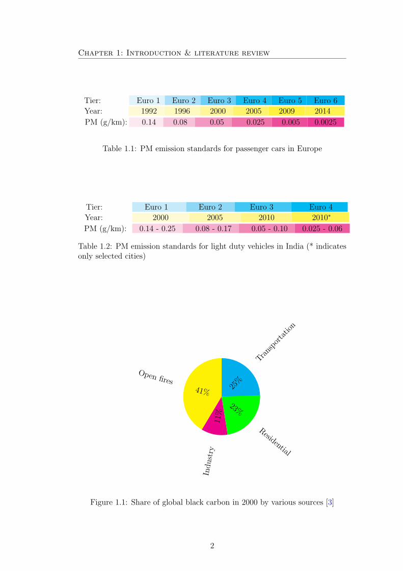
Table 1.1 depicts the European emission limits (g/km) for PM of passen-
ger cars. The equivalent norms in India for light duty vehicles are shown
in Table 1.2 (source: Wikipedia). Among these emitted particulate matters
from engines, the “soot” particles contribute the major part [2]. Soot is also
known as Black Carbon (BC). Soot particles are fractal-like aggregated prod-
ucts of small spherical particles constituted with elementary and organic car-
bon. They are important and inevitable products of combustion processes
(fuel-rich, incomplete combustion).
The main sources of soot or Black Carbon are depicted in the pie chart
(Fig. 1.1). Most of the soot is produced through open biomass burning fol-
lowed by automobiles engines, residential uses (e.g., cooking stoves) and from
industries [3].
Although soot has several adverse effects, in some practical combustion
1
Chapter 1: Introduction & literature review
Tier: Euro 1 Euro 2 Euro 3 Euro 4 Euro 5 Euro 6
Year: 1992 1996 2000 2005 2009 2014
PM (g/km): 0.14 0.08 0.05 0.025 0.005 0.0025
Table 1.1: PM emission standards for passenger cars in Europe
Tier: Euro 1 Euro 2 Euro 3 Euro 4
Year: 2000 2005 2010 2010∗
PM (g/km): 0.14 - 0.25 0.08 - 0.17 0.05 - 0.10 0.025 - 0.06
Table 1.2: PM emission standards for light duty vehicles in India (* indicatesonly selected cities)
25%
Transportation
41%
Open fires
11%
Industry
23%
Residential
Figure 1.1: Share of global black carbon in 2000 by various sources [3]
2
Chapter 1: Introduction & literature review
systems such as in glass furnaces soot formation is useful and important since it
enhances the heating through radiation. The distinction between soot or black
carbon and carbon black is vague in literature. Most types of commercially
produced carbon black contain more than 97% elemental carbon, whereas
soot/black carbon usually contains a lesser percentage of elemental carbon.
Carbon black is currently one most commercially significant product with an
annual production of 8.1 million tons. It finds its applications in automobile
tires, rubber, plastic products and in printing inks. More recent applications
include the use of carbon nanoparticles as a catalyst or catalyst support [4].
On the negative side, the recent research findings blame BC (soot) as one of
the significant contributors to global warming immediately after CO2, and any
measure to control the emission of soot will have an immediate effect on the
global warming since the life time of soot is shorter (a few days) than that of
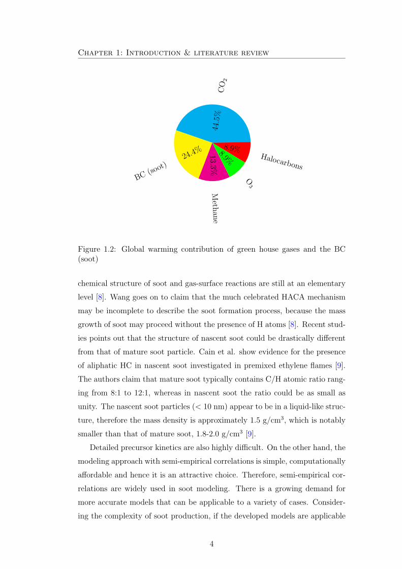
CO2 [5] (several years). In Fig. 1.2 the percentage of global warming ascribed
to different green house gases and BC is shown [6, 7]. The Intergovernmental
Panel on Climate Change (IPCC) estimates rank both BC and methane on
same level in their contribution to global warming (BC≈0.448; methane≈0.498
W/m2). In recent years scientists increasingly believe that BC contribution
may be very high (0.913 W/m2) and that the exact quantitative measure of
BC content in the atmosphere is difficult (values shown in Fig. 1.2 are for
2005).
There have been numerous studies during the last decades to understand
soot formation and its evolution. Nevertheless, many questions remain un-
solved due to the tremendous complexity of this process, involving gas-phase
and surface kinetics, coupled with turbulence, large heat transfer by radiation
and intricate interactions between the particles. There has been significant
improvement in isolated modeling aspects of soot formation. Several studies
aiming at quantitative prediction of soot particles were successful, at least
for simple fuels. Prediction of soot from complex fuels and in complex process
conditions such as in automobile engines is still extremely difficult, demanding
tremendous amount of modeling and computational efforts.
The existing phenomenological descriptions still do not explain completely
the sooting phenomena. For e.g., models for soot nucleation, evolution of the
3
Chapter 1: Introduction & literature review
44.5%
CO
2
24.4%
BC(so
ot)
13.3%Meth
ane
8.9%
O3
8.9%Halocarbons
Figure 1.2: Global warming contribution of green house gases and the BC(soot)
chemical structure of soot and gas-surface reactions are still at an elementary
level [8]. Wang goes on to claim that the much celebrated HACA mechanism
may be incomplete to describe the soot formation process, because the mass
growth of soot may proceed without the presence of H atoms [8]. Recent stud-
ies points out that the structure of nascent soot could be drastically different
from that of mature soot particle. Cain et al. show evidence for the presence
of aliphatic HC in nascent soot investigated in premixed ethylene flames [9].
The authors claim that mature soot typically contains C/H atomic ratio rang-
ing from 8:1 to 12:1, whereas in nascent soot the ratio could be as small as
unity. The nascent soot particles (< 10 nm) appear to be in a liquid-like struc-
ture, therefore the mass density is approximately 1.5 g/cm3, which is notably
smaller than that of mature soot, 1.8-2.0 g/cm3 [9].
Detailed precursor kinetics are also highly difficult. On the other hand, the
modeling approach with semi-empirical correlations is simple, computationally
affordable and hence it is an attractive choice. Therefore, semi-empirical cor-
relations are widely used in soot modeling. There is a growing demand for
more accurate models that can be applicable to a variety of cases. Consider-
ing the complexity of soot production, if the developed models are applicable
4
Chapter 1: Introduction & literature review
for well-defined flow conditions and for a given, simple fuel then this is already
a valuable contribution. Therefore, the first and the prime objective of the
present research work is to develop such semi-empirical soot models for turbu-
lent ethylene/air flames by using Computational Fluid Dynamics (CFD) and
optimization (CFD-O).
The second objective of this work is to predict the formation and evolu-
tion of TiO2 nanoparticles. For this purpose turbulent methane/oxygen/Ar
diffusion flames are considered with titanium-tetraisopropoxide (TTIP) as pre-
cursor. TiO2 nanoparticles have a wide range of applications such as in pig-
ments (white), photo-catalysis, sunscreens and solar cells. The flame synthesis
of nanoparticles such as TiO2 involves introduction (injection) of a precursor
dopant, in a gaseous or liquid state to the combustion system (flame) with the
help of a carrier gas. The precursor decomposes at given flame conditions and
forms nuclei (a few nanometers in size). Depending on process conditions the
further evolution of nanoparticles occurs due to molecular growth, oxidation
and aggregation.
The question may arise how these two processes (soot and TiO2) are re-
lated? The mechanisms controlling formation and evolution of both soot and
the commercial nanoparticles share common similarities. Both involve the
formation of a condensed phase material, nucleation, surface growth of the
particles and the subsequent aggregation into fractal structures. As a conse-
quence the employed modeling approach is also similar. In fact, the consider-
able experience gained in soot modeling helped many researchers to advance
in the modeling of commercial nanoparticles. Experimentally, both processes
have been investigated with the same diagnostic techniques such as laser in-
duced incandescence (LII) and transmission electron microscopy (TEM) [8].
Therefore, it is appropriate to study them together.
The present numerical study employs systematically the CFD solver Ansys-
Fluent for solving the gas-phase governing equations. The particle-phase Pop-
ulation Balance Equations (PBE) are transformed to moment transport equa-
tions and solved through moment-based methods. These methods are im-
plemented in our group into the CFD solver by using in-house user-defined
functions (UDF). The detailed description of the gas-phase and the particle
5
Chapter 1: Introduction & literature review
phase models employed in the present work are presented in Chapter 3.
The evolution of the particle phase (soot or TiO2) PBE is handled by
Quadrature Method of Moments (QMOM) and Direct Quadrature Method of
Moments (DQMOM). Moment-based methods have been proven to be accurate
for predicting the first moments of a variety of particle size distributions (PSD).
Additionally, they require much less computational time compared with a di-
rect solution of the PBE or with sectional methods. QMOM/DQMOM appear
very attractive since optimization can only be carried out when each individ-
ual simulation is relatively fast (at most a few hours of computing time). A
complete description of the moment-based methods employed in the present
work is given in Chapter 2.
Initial studies involved the use of semi-empirical soot models from litera-
ture. These models, which are called “original soot models” throughout this
study are tested on 4 different turbulent ethylene/air flames. Comparisons are
presented with published experimental data. It is shown later that these orig-
inal models were not capable of predicting accurately the soot volume fraction
(fv). These models are improved in this work through CFD-based optimiza-
tion (see Chapter 5). This numerical optimization relies on Computational
Fluid Dynamics to find the best possible model parameters. CFD-based op-
timization (CFD-O [10]) has been successfully applied to different configu-
rations involving heat transfer and flames within our research group in the
past [11, 12]. Based on this experience, a Genetic Algorithm (GA) coded in
the in-house optimization library OPAL (OPtimization ALgorithms) has been
combined with the industrial CFD solver Ansys-Fluent for the present study.
All details about CFD-O can be found in Chapter 4.
CFD-O has been performed in several cases starting with the simplest gas-
phase chemistry i.e., with equilibrium approximation. The predictions could
be improved in this case when compared to the original models, but were still
not satisfactory. Hence, in subsequent steps optimizations are performed by
considering more refined turbulent combustion models and considering soot
radiation. The finally obtained, optimized set of models leads to a signifi-
cant improvement of the predictions. The detailed analysis of the results is
presented in Chapter 5.
6
Chapter 1: Introduction & literature review
The numerical results concerning TiO2 nanoparticle formation in turbulent
CH4-O2 flames are presented in Chapter 6, before concluding. In the following
sections a brief literature review is proposed concerning the formation of soot
and TiO2 nanoparticles in flames.
1.2 Soot formation and modeling in turbulent
combustion systems: literature synthesis
Due to the adverse effects of soot on human health as a carcinogenic [13, 14]
and on the environment as one major global warming component [15, 16] with
a high impact on cloud cover and visibility [17], there have been numerous
studies during the last decades to understand soot formation and its evolution.
In spite of this the chemical mechanism of soot formation is still not very
clearly understood. The overview of the literature shows that the most am-
biguous process in soot modeling is nucleation on which much focus needs to
be made. Different soot inception routes can be found. Among them HACA
mechanism (H-abstraction/C2H2-addition: PAH1 route) is the most widely
accepted assumption in the literature. Some PAH molecules decompose and
form small aliphatic HCs which in turn form acetylene molecules. These PAH
molecules further grow in their size in 3-dimensional structure due to the se-
quential chain reaction with the acetylene molecules and form nascent soot
particles. These acetylene molecules also provide major contribution for fur-
ther growth of the soot particles. Shock tube experiments are typically used
to analyse the chemical mechanisms of soot formation.
Frenklach and co-workers discussed the chemical mechanism of soot for-
mation in several articles. Accordingly, the formation of first aromatic ring
in the non-aromatic fuels (e.g., ethylene as in the present study) begins usu-
ally with vinyl addition to acetylene [18]. Once the first aromatic ring is
formed, they grow in their size by a sequential two-step: H-abstraction which
activates the aromatic molecules, and acetylene addition which propagates
molecular growth and cyclization of PAHs as depicted in Fig. 1.3. Now these
1polycyclic aromatic hydrocarbons
7

Chapter 1: Introduction & literature review
_
2
2
CC
CC
+ H+
H
H+
+ H22
C2
H_
H
_
H
2+C 2
H2
H
H
C
Figure 1.3: H-abstraction-C2H2-addition reaction pathway of PAH growthtaken from [18]
formed macro molecules (PAH) in turn coagulate and form dimers, trimers
and tetramers and so on in three dimensional structures. Beginning with the
dimers the forming clusters were assumed to be in solid phase (nuclei) and al-
lowed to add and lose mass by surface reaction (growth and oxidation) [18, 19].
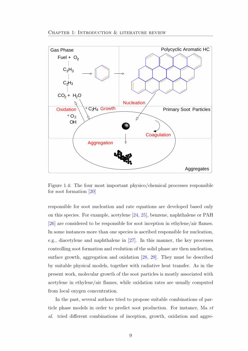
The widely accepted soot formation and evolution model as depicted in
[20] is shown in Fig. 1.4. This mechanism builds on top of that described by
Frenklach and co-workers [18].
Soot models are often classified into 3 different groups [21]: i) empirical
ii) semi-empirical and iii) kinetic soot models. While empirical models do
not allow detailed predictions, kinetic soot models are obviously best suited to
describe all the complex pathways leading from the fuel to the final particles. A
detailed modeling of soot formation based on polycyclic aromatic hydrocarbon
(PAH) concentration is given for instance in [22]. Nevertheless, such models are
difficult to be employed in real, three-dimensional flames of practical interest,
due to the considerable computational time required by the simulations [23].
As a consequence, semi-empirical models are mostly used at present and are
therefore the target of this work. They involve less computational effort by
simplifying all kinetic aspects. Usually, one single chemical species is deemed
8
Chapter 1: Introduction & literature review
C 4
2 2OCO + H
2 3C H
C3H3
Fuel + O2
OH
Aggregates
+
Polycyclic Aromatic HCGas Phase
ParticlesOxidation Primary SootNucleation
+ 2O2H Growth
Coagulation
Aggregation
Figure 1.4: The four most important physico/chemical processes responsiblefor soot formation [20]
responsible for soot nucleation and rate equations are developed based only
on this species. For example, acetylene [24, 25], benzene, naphthalene or PAH
[26] are considered to be responsible for soot inception in ethylene/air flames.
In some instances more than one species is ascribed responsible for nucleation,
e.g., diacetylene and naphthalene in [27]. In this manner, the key processes
controlling soot formation and evolution of the solid phase are then nucleation,
surface growth, aggregation and oxidation [28, 29]. They must be described
by suitable physical models, together with radiative heat transfer. As in the
present work, molecular growth of the soot particles is mostly associated with
acetylene in ethylene/air flames, while oxidation rates are usually computed
from local oxygen concentration.
In the past, several authors tried to propose suitable combinations of par-
ticle phase models in order to predict soot production. For instance, Ma et
al. tried different combinations of inception, growth, oxidation and aggre-
9

Chapter 1: Introduction & literature review
gation models in order to determine the best parameters for a non-premixed
ethylene/air flame [26]. Three different kinds of inception models (acetylene in-
ception route, the PAH inception route, and the naphthalene inception route),
three types of surface area functions for growth, three different coagulation
constants and finally three expressions of soot oxidation were investigated.
Zucca et al. proposed another model combination for the same type of flames,
again validated against experimental results [30]. Being more recent, the model
formulation presented in [30] has been retained as initial solution for the op-
timization process described in what follows. Even if such studies have led
to a significant improvement in understanding and predicting soot formation,
available models have yet to yield satisfactory comparisons against all avail-
able experimental data [31, 32]. There is thus a clear need for more accurate
prediction models, applicable to a wide range of flow and operating conditions.
First computational studies in our group concerning predictions of soot vol-
ume fraction [33] have demonstrated that the nucleation and oxidation models
play a first-order role for typical flame configurations, followed by molecular
growth and finally aggregation processes. Therefore, nucleation and oxidation
parameters are first retained in the following optimization.
Radiative heat transfer is significant in most combustion processes. Due
to the diversity of involved combustion products, to the complexity of obtain-
ing their radiative properties and to the coupling with turbulent flows, the
development of suitable radiation models is a challenge [34]. Selected gaseous
species (notably H2O and CO2) and particles (here soot) are the major contrib-
utors to radiation. Among those, soot particles are by far the most important
radiating product in sooting flames, emitting in a continuous spectrum in the
visible and infrared regions [35].
As explained earlier, when modeling soot formation in practical systems,
semi-empirical approaches are mostly used. Involved particulate models (nu-
cleation, growth. . . ) are all non-linear functions of temperature. Due to this
strong two-way coupling between soot and temperature, it is important to
model radiative heat transfer with a sufficient accuracy, while keeping accept-
able computational times. However, this is a real challenge since accurate radi-
ation models require a large amount of computing times, while simple models,
10

Chapter 1: Introduction & literature review
as considered in the present study, do not always lead to correct predictions.
An accurate evaluation of radiative heat transfer in turbulent flames is
extremely difficult due to three main challenges. First, it is difficult to ob-
tain numerically a correct solution of the radiative transfer equation (RTE), a
five-dimensional integro-differential equation. Secondly, the spectral behavior
of the radiating species and the spectral integration of the equations lead to
many problems. Finally, the evaluation of turbulence/radiation interactions
is unsolved, in particular for steady RANS simulations [36]. Additionally, the
soot particle size distribution (PSD) impacts radiation in sooting flames, but
this PSD is mostly not known with a good accuracy. The shape of the soot
particles also influences radiation [37], even if they are usually assumed spher-
ical. All these open issues lead to implementation difficulties in existing CFD
codes. Even with a successful implementation, the resulting computational
times prevent using truly accurate models for most practical configurations
of interest. As a consequence, it has been a common practice in the past to
invoke the optically thin approximation and to assume the medium to be grey
[19, 25, 38] when simulating turbulent burners, and we will keep the same
hypothesis.
An analysis of existing soot radiation models (e.g., [39, 40]) shows that
there is still a high level of uncertainty concerning the most appropriate model
description. As a consequence, this aspect is taken as well into account in
the optimization process. The detailed description about the various soot
radiation models considered in the present study can be found in Chapter 3
For the later optimization three different but simple soot radiation models
found in the literature and based on a grey medium and optically thin approx-
imation have been considered and compared. All three are implemented for
the simulation of nonpremixed turbulent ethylene/air flames. Four different
published experimental works (see Table 5.1, on page 69) are used to compare
the quality of the numerical predictions.
The particulate phase must always be solved in a coupled manner together
with the reactive Navier-Stokes equations. For this purpose, Netzell et al. used
sectional method for calculating PSD of soot in turbulent diffusion flames [41].
The authors considered in total 100 sections and emphasized the advantage
11
Chapter 1: Introduction & literature review
of this method as it delivers a PSD. Monte Carlo based methods have been
employed in many publications (see [42–45]) for modeling soot formation in
different flame configurations. Certainly, Monte Carlo methods also demand
high computational times. As an alternative, Method of moments (MOM) can
be used with interpolative closure for modeling soot formation in laminar and
turbulent flames [19, 20, 46, 47]. In order to obtain a computationally efficient
solution, QMOM/DQMOM have been coded for the present study into Ansys-
Fluent using User-Defined Functions. The quadrature approximation [48] used
in QMOM/DQMOM solves the closure problem associated with nonlinearities
in source terms such as growth and aggregation. With DQMOM, the PBE sim-
plifies into a set of algebraic equations with few additional transport equations
[49]. For example, if we consider 2 nodes for the quadrature approximation
as in the present project, only 4 transport equations must be solved in both
QMOM/DQMOM thus speeding up the computations compared to a direct
solution of the PBE.
Four different turbulent non-premixed ethylene/air flames [50–53] have
been considered for validation purposes in this work. The first flame [50]
is employed to determine the optimal set of model parameters by comparing
the obtained fields of temperature and soot volume fraction. The generality
of optimal model is then checked by comparison with three other flames [51–
53]. All results concerning optimization and validation for soot predictions are
discussed in Chapter 5
1.3 Literature on the synthesis of TiO2 nanopar-
ticles in flames
The scientific and commercial interest in the manufacture of nanoparticles
has increased many folds since the importance of nanoparticles is now well
documented for numerous applications. The special properties of nanoparti-
cles make their use attractive in several regards. These special properties are
mainly due to the large surface to volume ratio of nanoparticles. For a particle
of about 4 nm, half of the molecules forming the nanostructure are actually at
12
Chapter 1: Introduction & literature review
the surface with consequences for the lattice structure. This causes dramatic
changes in the physical and chemical properties (like melting point, magnetic
and optical properties) of nanomaterial compared to the same bulk material
[54].
Extensive research is going on in varied fields of science to analyse the appli-
cability of nanoparticles. Nanoparticles are excellent catalysts and have been
used in synthesis of several components. Major applications of nanoparticles
are summarized as follows:
• Ceramics - TiO2, Al2O3, Fe2O3
• Catalysis - VaO2-TiO2, Pt/Ba/Al2O3, DeNOx, TiO2-SiO2 epoxide cata-
lysts, Pd/Al2O3, KF/CaO (in bio-diesel production), TiO2
• Fiber optics - SiO2
• Nano-magnetic material, data storage - Fe2O3
• Super conducting materials - Sn, Al, CeCo2,
• Fuel cells - with nano-catalysts, electrolyte (gadolinia for solid oxide fuel
cell), nano-composites for gas barriers, Carbon nano tubes (CNT)
• Electronics - sensors SnO2, titania based
• Chemical - mechanical polish and in coatings
• Medical applications - drug delivery and diagnostics - polymer nanopar-
ticles for oral anticancer drug delivery, pulmonary vaccines, diabetic,
orthopaedic, dental and nutritional products
• Pigments - TiO2, carbon black
• Flowing aids - SiO2 for pharmaceuticals and cosmetics
• Inorganic membranes and sunscreens - ZnO, TiO2
• Solid rocket propellants - Al particles
13

Chapter 1: Introduction & literature review
Despite the wide spread applications of nanoparticles, adverse effects of
fine particles on health and environment are also worthy of special research. A
clear knowledge on health/environment effects of nanoparticles is still limited.
Several studies document the adverse effects of different nanoparticles [55–57].
Gas-phase flame synthesis processes are often chosen to produce nanopar-
ticles, in large quantities as it is in general cleaner, more energy-efficient,
environmentally cleaner and easier [58, 59]. This process also does not in-
volve expensive steps of solid-liquid separation, washing and drying as in wet
chemistry processes. As a consequence flame reactors are one of the most
common methods used for the production of high-purity nanoscale powders in
large quantities, especially for silica, titania, and alumina. There are several
industrial-scale plants operated world wide that already produce several mil-
lion tons of nanoparticles per year. For instance, Degussa (now Evonik) has
developed to maturity the large-scale production of nanostructured zinc oxide,
based on gas-phase synthesis for use as a UV filter in sunscreens.
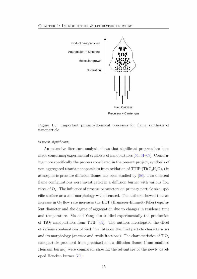
The flame synthesis of nanoparticles involves introduction (injection) of
a precursor dopant in a gaseous or liquid state in to the combustion system
(flame) with the help of a carrier gas. This precursor decomposes (mostly due
to oxidation) at given flame conditions and forms nuclei (a few nanometers
in size). Depending on process conditions further evolution of nanoparticles
occurs due to molecular growth, oxidation and aggregation. When formation
process of commercial nanoparticles is compared with soot formation, the ox-
idation is found to be rarely significant in the former case. The basic steps of
particle formation and growth from gas to particle conversion in a flame are
shown in Fig. 1.5.
Flame synthesis of various nanoparticles, like SiO2, TiO2, and SnO2, mixed
oxides or nanocomposites such as V2O5/Al2O3, Fe2O3/SiO2 have been dis-
cussed by several authors in recent years, for instance in [54, 58, 60]. Process
chemistry, transport phenomena, particle dynamics and nanoparticle appli-
cations have been discussed in detail in these works. Accordingly, process
variables such as material properties, flame configuration, precursor type, tem-
perature, oxidant composition, mixing, are known to play an essential role for
final product characteristics. According to the literature, process temperature
14
Chapter 1: Introduction & literature review
������������������������������������
������������������������������������
��������������
��������������
������������������������������������
������������������������������������
����������������������������
����������������������������
Precursor + Carrier gas
OxidizerFuel,
Nucleation
Aggregation + Sintering
Product nanoparticles
Molecular growth
Figure 1.5: Important physico/chemical processes for flame synthesis ofnanoparticle
is most significant.
An extensive literature analysis shows that significant progress has been
made concerning experimental synthesis of nanoparticles [54, 61–67]. Concern-
ing more specifically the process considered in the present project, synthesis of
non-aggregated titania nanoparticles from oxidation of TTIP (Ti(C3H7O)4) in
atmospheric pressure diffusion flames has been studied by [68]. Two different
flame configurations were investigated in a diffusion burner with various flow
rates of O2. The influence of process parameters on primary particle size, spe-
cific surface area and morphology was discussed. The authors showed that an
increase in O2 flow rate increases the BET (Brunauer-Emmett-Teller) equiva-
lent diameter and the degree of aggregation due to changes in residence time
and temperature. Ma and Yang also studied experimentally the production
of TiO2 nanoparticles from TTIP [69]. The authors investigated the effect
of various combinations of feed flow rates on the final particle characteristics
and its morphology (anatase and rutile fractions). The characteristics of TiO2
nanoparticle produced from premixed and a diffusion flames (from modified
Hencken burner) were compared, showing the advantage of the newly devel-
oped Hencken burner [70].
15
Chapter 1: Introduction & literature review
Pratsinis and co-workers discussed in many publications the experimental
synthesis and modeling of various nanoparticles. TiO2 production has been
documented more particularly in [1, 62, 71]. Coflow burners of 3 different di-
mensions have been used for various precursors, fuel and oxidizer flow rates.
Synthesis of TiO2 nanoparticles using TTIP as precursor was investigated ex-
perimentally and numerically by [72]. Using a sectional method, particle size
distribution (PSD), average primary particle size and geometric standard de-
viation were analyzed for a wide range of process parameters and validated by
experiments. Sunsap et al. studied experimentally in a diffusion flame reac-
tor the effect of oxidizer, fuel flow rates and filter position on specific surface
area, primary and secondary particle sizes, morphology, phase composition
and crystallite size of TiO2 nanoparticles [73]. The same authors have stud-
ied computationally the influence of process parameters (various flow rates of
O2 and CH4) on production (deposition rate) of TiO2 nanoparticles in the
diffusion flame reactor during CH4 combustion.
The focus of many experimental investigations found in the literature is
mainly set on studying the influence of selected process parameters such as
flow rates of fuel/precursor/oxidizer and flow configuration on final particle
characteristics for a fixed burner. This experimental process optimization is
quite costly and time-consuming. A similar optimization based on simulations
would be more cost effective and faster, if efficient and accurate physicochem-
ical and numerical models and available to describe the target properties of
TiO2 particles.
In [74], the production of TiO2 nanoparticles in CH4-air diffusion flames
using TiCl4 as precursor is considered, while [75] investigates a premixed flame
with TTIP as precursor. The numerical results are found in fair agreement
with experimental data in both studies. In both studies the authors employed
the CFD solver Ansys-Fluent, as done here. Synthesis of TiO2 nanoparticles
by TTIP oxidation in a premixed methane-oxygen flame has been studied
in [76]. A moving sectional method is employed accounting for gas phase
chemical reactions, coagulation, surface growth and sintering. Influence of
surface shielding and surface energy on growth mechanisms during titania
generation has been modeled in the oxidation of TiCl4 by [77].
16
Chapter 1: Introduction & literature review
Yu et al. combined Computational Fluid Dynamics with particle kinetics
to study the effect of precursor loading on non-spherical TiO2 nanoparticle
synthesis from TTIP in a diffusion flame reactor [59]. Same authors described
numerical evaluation of TiO2 nanoparticle synthesis from TiCl4 in diffusion
flame under similar lines to the earlier work [78]. Sung et al. studied the TiO2
nanoparticle production from a non-premixed flame configuration with TiCl4
as precursor [79] by taking into account the nucleation and aggregation. In the
present study, the molecular growth effect is additionally taken into account.
TiO2 formation by oxidation of TTIP and TiCl4 has been studied numer-
ically for producing narrower PSD of aerosols by controlling the reactions on
the particle surface in [80]. The authors explored the effect of various process
parameters such as pressure, temperature and initial precursor molar fraction
on surface growth reaction of titania particles. Volume-based size and standard
deviations (σg) were compared for all the cases. It is shown that increasing ei-
ther process temperature, pressure or initial precursor molar fraction enhanced
surface growth, which resulted in a narrower PSD. According to these authors
further improvements are possible until obtaining nearly monodisperse PSD
(σg < 1.3).
Although there is good progress in developing and commercially producing
different nanoparticles for various applications through experimental analy-
sis, the modeling approach is still poorly developed. Much kinetic and ther-
mochemical data is still missing. While modeling nanoparticle formation in
flames, one usual but important assumption is the decoupling of the gas-phase
chemistry from the particle-phase chemistry, thus avoiding the complications
associated with heterogeneous kinetic data between the phases [58]. Includ-
ing detailed particle phase kinetics in the modeling is of course desirable and
should give more accurate predictions. But, at the same time it involves huge
computational efforts. In most cases, authors assume a single-step, global re-
action to describe nuclei formation from the precursor solution. This is also
the approach retained here.
All these studies rely on a manual, trial-and-error strategy in order to im-
prove the process. Moreover, they always consider a fixed burner geometry.
Optimizing particle properties on a short time scale, with a higher efficiency
17
Chapter 1: Introduction & literature review
and taking all relevant parameters into account (including burner and flame
configuration) is still very challenging. For this, coupling simulations with
optimization techniques would be far more efficient [10, 12]. Applying this
optimization technique for producing nanoparticles from flame reactors is the
ultimate purpose of this project. As a first step, in the present work, a manual
optimization of process conditions and geometries is attempted, with the ob-
jective of obtaining a lower mean diameter (dmean), a higher volume fraction
(fv) and a narrower PSD (minimizing σg, tending towards a monodisperse
case).
In the following section, a review of literature on application of moment-
based methods (specifically QMOM and DQMOM) in various fields of science
is given.
1.4 Application of QMOM/DQMOM in dif-
ferent physical and chemical processes
The complete description of these moment-based methods (QMOM and DQ-
MOM) is given later in Chapter 2. In this section only the application of
these methods to different fields from literature is discussed. As stated earlier
the evolution of the solid phase is handled by PBE and needs to be solved
along with Navier-Stokes equations in a variety of chemical engineering prob-
lems. QMOM and DQMOM have been applied and validated in a wide range
of applications such as fluidization, crystallization, precipitation, combustion,
etc.
For instance, QMOM/DQMOM has been implemented to study polydis-
persed gas-solid fluidized beds. DQMOM was used by Fan et al. to model the
aggregation and breakage process in fluidized bed and has been coupled to a
CFD code for this purpose [81]. In this case each quadrature node represents
a distinct solid phase and thus is convected with its own velocity, as a multi-
fluid CFD code is employed. Therefore, it is an important improvement when
compared with QMOM. The authors have studied the effect of the number of
nodes N (2, 3 and 4) and compared the results. From the results the authors
18

Chapter 1: Introduction & literature review
recommend the kinetic theory kernel and 3 quadrature nodes (N = 3) for
fluidized bed reactors.
The importance of particle mixing and segregation were studied for a bi-
nary system with a continuous PSD by Fan and Fox [82]. In this work, the
authors used a multi-fluid model based on the Euler-Euler approach and DQ-
MOM to describe particle segregation in polydispersed fluidized beds. Model
predictions are validated with available experimental and simulation data. The
results showed that, when the PSD is narrow or the superficial gas velocity
is high, less nodes are needed. For a wide PSD with significant segregation,
at least 3 quadrature nodes are needed for accurate results. One important
limitation of QMOM/DQMOM was recently highlighted by Mazzei [83]. The
author studied the dynamics of two inert polydisperse fluidized suspensions
which are initially segregated (dense system). The author reveals an impor-
tant limitation, that QMOM/DQMOM fails to properly model the diffusion
in real space. This is because diffusion is caused by the particle population
being continuously distributed over the internal coordinates; this continuity
no longer exists when the NDF is approximated with a quadrature formula,
since doing so seperates the distribution into a finite number of classes (in
the extreme case of one class, all the particles would have the same internal
coordinates, which clearly kills diffusive fluxes) [83].
Zucca et al. validated DQMOM approach in the soot formation modeling of
turbulent ethylene/air diffusion flame [30]. In this case the DQMOM algorithm
has been implemented in Ansys-Fluent. Nucleation, growth, aggregation and
oxidation were considered as the particle phase source terms. With a mono-
variative PBE and 2 nodes of the distribution, just 4 additional scalar transport
equations need to be solved. Recently the same authors applied DQMOM to
bi-variative PBE with particle volume and area as the internal co-ordinates [84]
and demonstrated its simplicity in extending it to multi-variate PBEs. Results
are shown considering 2 and 3 quadrature nodes (N = 2, 3). Comparisons
were also made with Monte-Carlo Method (MCM). A pseudo bivariate PBE
was also used to describe the soot formation modeling in turbulent flames by
Marchisio under similar lines [84].
The choice of moments also plays a significant role in the accuracy of
19

Chapter 1: Introduction & literature review
moment methods (QMOM/DQMOM) and certain choices of moments will
minimize the condition number of matrix A (see Section 2.4.1). QMOM and
DQMOM approaches were validated by Upadhyay and Ezekoye [85] using an
analytical solution by considering a simplified problem of aerosol settling and
diffusion between infinite parallel plates. The authors investigated the accu-
racy of the solutions by considering different sets of moments of the initial
NDF and concluded that the solution to the moment equations depends on
the initial choice of moments. Therefore, it is possible to improve the accu-
racy of the solution by an optimal choice of moments. According to Fox, poor
choices for the moment set can lead to non-unique abscissas and even negative
weights [86]. According to Zucca et al., proper selection of the moments is
necessary for the stability and the lower order moments benefit most from a
better condition of the matrix [84].
McGraw and co-workers extended the application of QMOM to bivariate
PBE (representing particle volume and area) for modeling particle coagulation
and sintering processes [87]. The calculations were performed with N = 3 and
N = 12 nodes. Please note that in the later case one needs to consider 36
moments. Therefore the selection of moments and the calculations become
quite challenging. Fox [88] applied DQMOM to the same problem and the
published QMOM results were reproduced demonstrating the simplicity of
DQMOM over the previously published work on QMOM. It is found that the
coagulation and sintering kernels used in this test case are easily handled by
lower-order moment methods, and are relatively insensitive to the choice of
bivariate moments used for DQMOM.
Moment methods are also increasingly gaining importance in the modeling
of commercial nanoparticle products from flame synthesis route. Due to the
complex nature of the physico-chemical models involved in the flame synthesis
of nanoparticles, moment methods appear attractive as they are simple and
less expensive. TiO2 nanoparticle synthesis has been studied by Yu et al. in
CH4/O2 diffusion flames with TTIP as the precursor and Ar as the carrier gas.
The authors employed QMOM and obtained the first few moments of the NDF,
area concentration and the primary particle diameter [59]. The authors also
used QMOM in similar lines for the production of TiO2 particles from CH4/O2
20
Chapter 1: Introduction & literature review
diffusion flames with TiCl4 as the precursor and Ar as the carrier gas. They
studied the effect of inlet precursor loading on the particle phase properties
such as particle number, size, specific surface area (SSA) and shape [78]. Sung
et al. studied the TiO2 nanoparticle production from a non-premixed flame
configuration with TiCl4 as precursor [79]. The NDF is tracked by QMOM
involving only nucleation and aggregation and ignored the sintering and growth
effects. Only monovariate PBE is considered in all these applications.
Sprays are common in many industrial combustion applications such as
diesel engines. Fox et al. applied DQMOM and multi-fluid method to solve
Williams spray equation and compared the two approaches for various test-
cases [89]. The other key point of the study is a detailed description of the
limitations associated with each method, thus giving criteria for their use as
well as for their respective efficiency. As far as coalescence phenomena are
concerned, the efficiency of DQMOM has been shown to be better than the
multi-fluid model due to its limited numerical diffusion in the size phase space.
The authors have also shown that for the bimodal distribution function and
as for as the evaporation process is concerned, DQMOM is comparable to
the multi-fluid model. An interesting limitation of the moment methods has
been pointed out by Massot et al., [90]. According to the authors, a drift
velocity, i.e., the rate of change due to continuous phenomena affecting the
internal coordinate, has to be taken into account. It is particularly important
when there exists a negative drift velocity, such as evaporation of droplets or
oxidation of soot particles. The authors proposed a modified formulation for
DQMOM to model such instances. Very recently QMOM was applied to solve
bivariate PBE in ethanol-fueled spray combustors [91].
Crystallization is an other application where the particle phase (crystals)
co-exists with the mother liquor. Barium sulphate crystallization has been
studied in turbulent flows by using SMOM in [92]. In this case the authors
assumed a priori a crystal size distribution (CSD) with a Gaussian shape and
reconstructed the distribution. PBM has been applied to batch crystallization
reactor in CFD codes by Wan and Ring [93]. A simple homogeneous system
with temporal variations, only one process at a time (nucleation only, growth
only etc.) has been considered. SMOM and QMOM were used to obtain the
21

Chapter 1: Introduction & literature review
first 6 moments and the predictions were compared with an analytical solution.
In contrast to this earlier study, several combinations of particulate processes
(nucleation, growth and dissolution; aggregation and breakage etc. ) have
been studied in an ideally mixed batch crystallization reactor by Qamar et al.
using QMOM [94].
There are several other moment based methods, for instance the method
of moments with interpolative closure (MOMIC) and the Finite size domain
Complete set of trial functions Method Of Moments (FCMOM). MOMIC was
widely used by Frenklach for soot particle formation in hydrocarbon combus-
tion flames [47, 95–97]. In MOMIC the fractional order moments are obtained
through interpolation among known whole-order moments. MOMIC was also
successfully implemented recently in a CFD code for the modeling of TiO2
nanoparticles evolution from TiCl4 oxidation [98]. FCMOM was applied and
validated for monovariate PBE [99, 100] and for bivariate PBE [101]. In FC-
MOM, the method of moments is formulated in a finite domain of the internal
coordinates and the particle size distribution function is represented as a trun-
cated series expansion by a complete system of ortho-normal functions. The
authors claim that FCMOM has several advantages. The solution of the PBE
obtained through the FCMOM provides both the moments and also the re-
constructed particle size distribution through a simple relation. The later can
be particularly important as the reconstruction of the PSD is a complex issue.
After having discussed the importance of soot and TiO2 nanoparticles and
existing literature on the subject, the next chapters present the computational
methods and models employed in the present project.
22

Chapter 2
Population Balance Equation
and Moment based methods
2.1 Introduction
Solution of the Population Balance Equation (PBE) is always a crucial step
in multiphase systems where the dispersed phase usually consists of solid or
liquid droplets. It is nearly impossible to get an analytical solution for practical
problems, although there exist analytical solutions for very simple, academic
processes [102]. Due to this, great amount of research is now being carried
out on solution techniques for the PBE in order to accelerate computations.
Several methods have been proposed by different researchers in this regard. To
list some of them : Method of classes or sectional methods, Monte Carlo (MC),
moment-based methods such as Quadrature Method Of Moments (QMOM) or
Direct Quadrature Method of Moments (DQMOM). There exist many other
methods like Finite Element Approach to PBE, that are not discussed here.
Every researcher has some reason to substantiate his or her approach and
some points that find loopholes in other methods. In the present chapter the
mathematical formulation and the application of moment-based methods are
discussed.
Population Balance Equation (PBE) is a continuity statement for the par-
ticle number density function (f). This f is a function written in terms of
internal and external co-ordinates [102]. Internal co-ordinates ξ come from
the property of the dispersed phase, such as particle diameter (length), area,
23
Chapter 2: Population Balance Equation and Moment basedmethods
volume, colour etc. External co-ordinates are physical space x (here bold phase
of ‘x’ signifies that x is a vector) and time t.
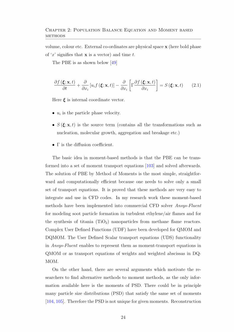
The PBE is as shown below [49]
∂f (ξ;x, t)
∂t+
∂
∂xi
[uif (ξ;x, t)]−∂
∂xi
[Γ∂f (ξ;x, t)
∂xi
]= S (ξ;x, t) (2.1)
Here ξ is internal coordinate vector.
• ui is the particle phase velocity.
• S (ξ;x, t) is the source term (contains all the transformations such as
nucleation, molecular growth, aggregation and breakage etc.)
• Γ is the diffusion coefficient.
The basic idea in moment-based methods is that the PBE can be trans-
formed into a set of moment transport equations [103] and solved afterwards.
The solution of PBE by Method of Moments is the most simple, straightfor-
ward and computationally efficient because one needs to solve only a small
set of transport equations. It is proved that these methods are very easy to
integrate and use in CFD codes. In my research work these moment-based
methods have been implemented into commercial CFD solver Ansys-Fluent
for modeling soot particle formation in turbulent ethylene/air flames and for
the synthesis of titania (TiO2) nanoparticles from methane flame reactors.
Complex User Defined Functions (UDF) have been developed for QMOM and
DQMOM. The User Defined Scalar transport equations (UDS) functionality
in Ansys-Fluent enables to represent them as moment-transport equations in
QMOM or as transport equations of weights and weighted abscissas in DQ-
MOM.
On the other hand, there are several arguments which motivate the re-
searchers to find alternative methods to moment methods, as the only infor-
mation available here is the moments of PSD. There could be in principle
many particle size distributions (PSD) that satisfy the same set of moments
[104, 105]. Therefore the PSD is not unique for given moments. Reconstruction
24

Chapter 2: Population Balance Equation and Moment basedmethods
of the PSD can be cumbersome. Several studies have successfully validated the
accuracy of the first few moments of the PSD [48, 93, 106, 107]. The accuracy
of higher order moments is still a subject of scientific discussion. Since the
objective of my research work is to successfully predict the mean properties of
the particle phase, in particular such as particle size and volume fraction fv,
the first moments should be sufficient to obtain these mean particle properties
with acceptable accuracy. If the internal co-ordinate is the diameter of the
particle, then the mean particle diameter is obtained through (µ1
µ0
) and the
third moment (µ3) directly gives the volume fraction fv, where µi represents
the ith moment. Hence, higher moments are not needed.
2.2 Solution of population balance equations
Among all the moment based methods, the standard method of moments
(SMOM) initially developed by Hulburt and Katz [103] is very simple but it
is only valid to specific cases. It is only valid when the transformed moment
transport equations are in closed form, i.e., all the terms in the transport
equation are described by known moments. Due to this it does not require
any additional approximation on the shape of the Particle Size Distribution
(PSD). For example if a “constant” growth rate or coagulation rate is assumed,
the moment transformation leads to a system of equations which are closed.
This means that the value of a given moment of the distribution is only related
to the value of lower order moments. In reality, real processes lead to unclosed
terms in most cases [48]. Due to this, the moment transformation results in
unclosed system of equations for which we need additional a priory approx-
imations on the shape of the PSD. These unclosed terms are very common
in practical applications since most of the processes are non-linear in nature.
Therefore, the difficulty in moment-based methods lies in representing this clo-
sure approximation in an acceptable manner. Since SMOM is not used in this
work apart for initialization, it is not described in more details. A description
of at least a few frequently used methods is the subject of the present chapter.
In practice, the proper choice of an initial guess is always very important
for the numerical stability of the solver. It is indeed well known that the mo-
25
Chapter 2: Population Balance Equation and Moment basedmethods
ments of the initial number density function (NDF) are a significant factor
for obtaining accurate and stable solutions from QMOM and DQMOM [85].
Therefore, following our own analysis, it is highly recommended that for all
complex processes where the system of equations are not closed initially, an
initial solution should be obtained with SMOM assuming corresponding sim-
plifications. Now, use this solution in the next step for initialisation of other
methods like QMOM/DQMOM. In this way it is possible to obtain suitable
and stable initial values. For example, when considering only nucleation and
molecular growth for soot/TiO2 particles as shown later, the moment trans-
formation results in a closed set of equations, which can be solved easily with
SMOM. Now, this initial solution makes a good guess to QMOM/DQMOM,
when we include the complex aggregation phenomena even if the system is
not closed now. In all the calculations of the present work this initialization
method has been employed.
In the subsequent sections the mathematical description of QMOM and
DQMOM are discussed. Applications of these moment-based methods for
various engineering problems has been discussed by citing examples from the
literature in Section 1.4.
2.3 Solution of population balance equations
using QMOM
McGraw first introduced QMOM, through which the moments of the PSD
are tracked in similar lines with SMOM. Initially, he used QMOM to describe
the sulphuric acid-water aerosol dynamics [48]. The method was later widely
applied and validated by Fox & Marchisio [106, 108–111]. QMOM was also
extensively used by other researchers for various problems [93, 94, 112].
In QMOM and DQMOM the number density function (NDF) f is repre-
sented with numerical quadrature, i.e., the distribution function is regarded
as the weight function [48]. This eliminates the closure problem associated
with moment transformation of the PBE involving complex terms (such as
Brownian aggregation kernel). Here, the unknown NDF is approximated with
26
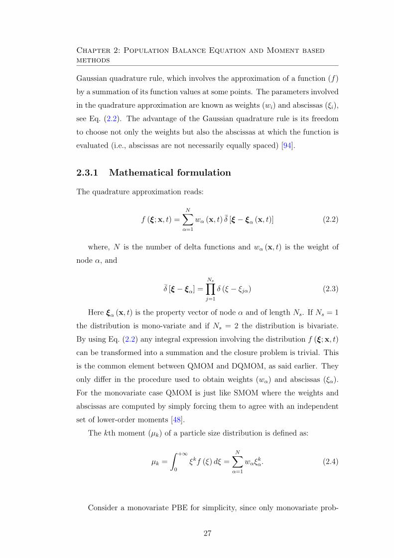
Chapter 2: Population Balance Equation and Moment basedmethods
Gaussian quadrature rule, which involves the approximation of a function (f)
by a summation of its function values at some points. The parameters involved
in the quadrature approximation are known as weights (wi) and abscissas (ξi),
see Eq. (2.2). The advantage of the Gaussian quadrature rule is its freedom
to choose not only the weights but also the abscissas at which the function is
evaluated (i.e., abscissas are not necessarily equally spaced) [94].
2.3.1 Mathematical formulation
The quadrature approximation reads:
f (ξ;x, t) =N∑
α=1
wα (x, t) δ [ξ − ξα (x, t)] (2.2)
where, N is the number of delta functions and wα (x, t) is the weight of
node α, and
δ [ξ − ξα] =Ns∏
j=1
δ (ξ − ξjα) (2.3)
Here ξα (x, t) is the property vector of node α and of length Ns. If Ns = 1
the distribution is mono-variate and if Ns = 2 the distribution is bivariate.
By using Eq. (2.2) any integral expression involving the distribution f (ξ;x, t)
can be transformed into a summation and the closure problem is trivial. This
is the common element between QMOM and DQMOM, as said earlier. They
only differ in the procedure used to obtain weights (wα) and abscissas (ξα).
For the monovariate case QMOM is just like SMOM where the weights and
abscissas are computed by simply forcing them to agree with an independent
set of lower-order moments [48].
The kth moment (µk) of a particle size distribution is defined as:
µk =
∫ +∞
0
ξkf (ξ) dξ =N∑
α=1
wαξkα. (2.4)
Consider a monovariate PBE for simplicity, since only monovariate prob-
27

Chapter 2: Population Balance Equation and Moment basedmethods
lems are considered later. Then, the moment transformation of the PBE
(Eq. 2.1) gives
∂µk
∂t+
∂
∂xi
[uiµk]−∂
∂xi
[Γ∂µk
∂xi
]=
∫∞
0
S (ξ;x, t) ξkdξ = Sk (2.5)
The right hand side of Eq. (2.5) includes all the mechanisms that bring
change in the number density function (f). For e.g., in the case of soot forma-
tion in hydro-carbon flames, these processes are nucleation, molecular growth,
oxidation and aggregation, where as in the case of TiO2 nanoparticles synthesis
from flames, oxidation is not considered since it is negligible.
2.3.2 Source term evaluation for the different processes
2.3.2.1 Nucleation (J):
For nucleation, a uniform distribution of particles of size 0 ≤ ξ ≤ ε has been
initially assumed, where, ε is the maximum size of the nuclei. The earlier
experimental studies from literature on ethylene diffusion flames which are
aimed at determining the soot primary particle size and volume fraction show
the possible range as ≈ 15 nm to ≈ 40 nm [113–115]. In the present work ε,
which is the maximum possible particle diameter of the nuclei is assumed to be
34 nm for soot particle modeling (as in a similar numerical study, [30]). For the
case of TiO2 particles modeling ε is approximated to be 1 nm3 after mannual
testing (please note that internal co-ordinate is volume in this case). Recently,
for TiO2 particles modeling in the group of Prof. Fox, authors assumed the
following range for particle nucleation 0.07 ≤ ξ ≤ 0.2 (ε) [79]. From the
definition of uniform distribution of size range a ≤ ξ ≤ b is equal to 1b−a
. From
the uniform distribution definition, Eq. (2.33) and from the nucleation rate
J (x, t):
Sk ≈ S(N)k =
∫ ε
0
ξk1
εJ (x, t) dξ (2.6)
Sk =εk
k + 1J (x, t) (2.7)
28
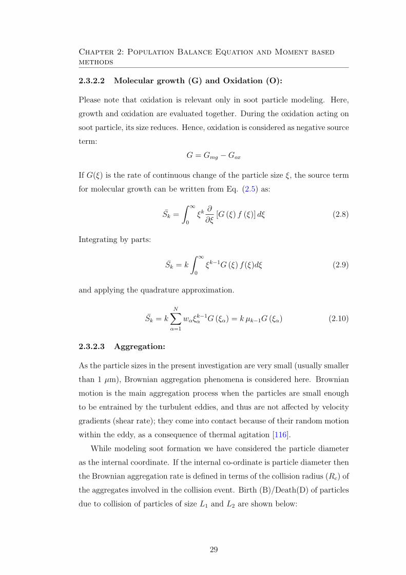
Chapter 2: Population Balance Equation and Moment basedmethods
2.3.2.2 Molecular growth (G) and Oxidation (O):
Please note that oxidation is relevant only in soot particle modeling. Here,
growth and oxidation are evaluated together. During the oxidation acting on
soot particle, its size reduces. Hence, oxidation is considered as negative source
term:
G = Gmg −Gox
If G(ξ) is the rate of continuous change of the particle size ξ, the source term
for molecular growth can be written from Eq. (2.5) as:
Sk =
∫∞
0
ξk∂
∂ξ[G (ξ) f (ξ)] dξ (2.8)
Integrating by parts:
Sk = k
∫∞
0
ξk−1G (ξ) f(ξ)dξ (2.9)
and applying the quadrature approximation.
Sk = k
N∑
α=1
wαξk−1α G (ξα) = k µk−1G (ξα) (2.10)
2.3.2.3 Aggregation:
As the particle sizes in the present investigation are very small (usually smaller
than 1 µm), Brownian aggregation phenomena is considered here. Brownian
motion is the main aggregation process when the particles are small enough
to be entrained by the turbulent eddies, and thus are not affected by velocity
gradients (shear rate); they come into contact because of their random motion
within the eddy, as a consequence of thermal agitation [116].
While modeling soot formation we have considered the particle diameter
as the internal coordinate. If the internal co-ordinate is particle diameter then
the Brownian aggregation rate is defined in terms of the collision radius (Rc) of
the aggregates involved in the collision event. Birth (B)/Death(D) of particles
due to collision of particles of size L1 and L2 are shown below:
29
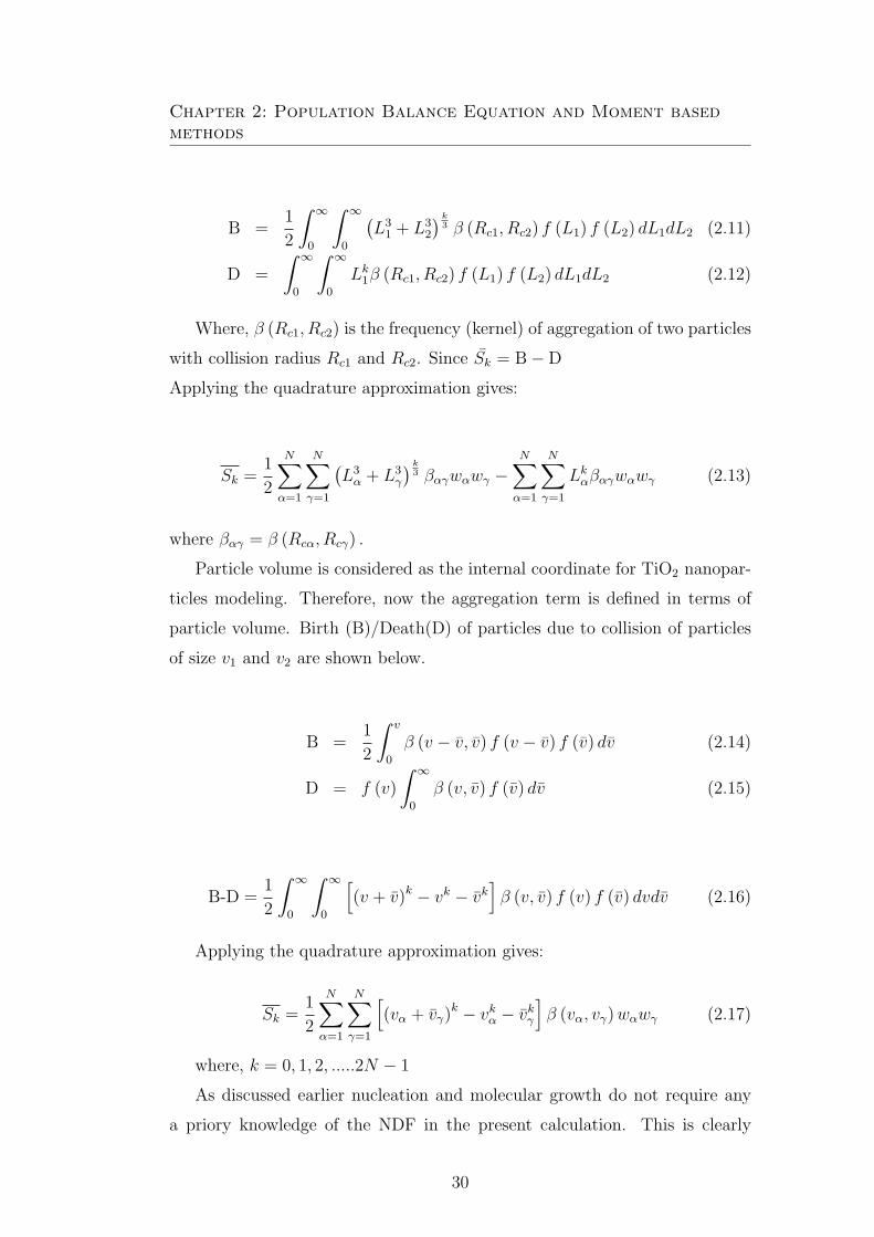
Chapter 2: Population Balance Equation and Moment basedmethods
B =1
2
∫∞
0
∫∞
0
(L31 + L3
2
) k3 β (Rc1, Rc2) f (L1) f (L2) dL1dL2 (2.11)
D =
∫∞
0
∫∞
0
Lk1β (Rc1, Rc2) f (L1) f (L2) dL1dL2 (2.12)
Where, β (Rc1, Rc2) is the frequency (kernel) of aggregation of two particles
with collision radius Rc1 and Rc2. Since Sk = B−D
Applying the quadrature approximation gives:
Sk =1
2
N∑
α=1
N∑
γ=1
(L3α + L3
γ
) k3 βαγwαwγ −
N∑
α=1
N∑
γ=1
Lkαβαγwαwγ (2.13)
where βαγ = β (Rcα, Rcγ) .
Particle volume is considered as the internal coordinate for TiO2 nanopar-
ticles modeling. Therefore, now the aggregation term is defined in terms of
particle volume. Birth (B)/Death(D) of particles due to collision of particles
of size v1 and v2 are shown below.
B =1
2
∫ v
0
β (v − v, v) f (v − v) f (v) dv (2.14)
D = f (v)
∫∞
0
β (v, v) f (v) dv (2.15)
B-D =1
2
∫∞
0
∫∞
0
[(v + v)k − vk − vk
]β (v, v) f (v) f (v) dvdv (2.16)
Applying the quadrature approximation gives:
Sk =1
2
N∑
α=1
N∑
γ=1
[(vα + vγ)
k − vkα − vkγ
]β (vα, vγ)wαwγ (2.17)
where, k = 0, 1, 2, .....2N − 1
As discussed earlier nucleation and molecular growth do not require any
a priory knowledge of the NDF in the present calculation. This is clearly
30
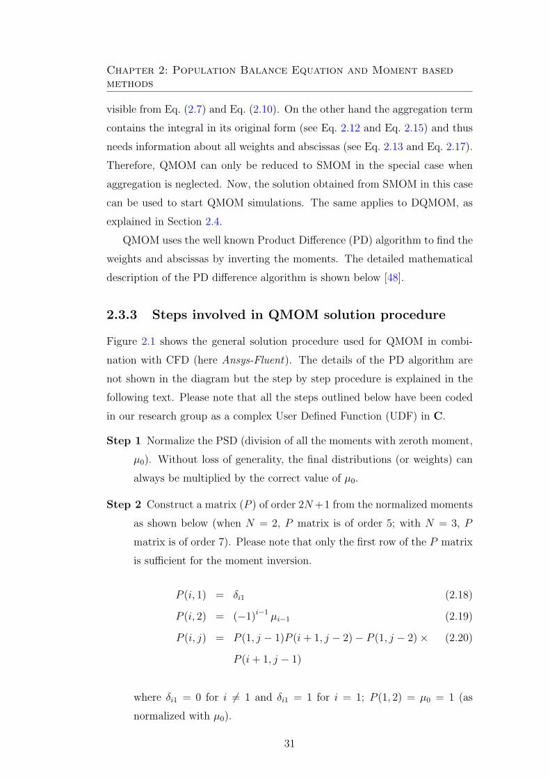
Chapter 2: Population Balance Equation and Moment basedmethods
visible from Eq. (2.7) and Eq. (2.10). On the other hand the aggregation term
contains the integral in its original form (see Eq. 2.12 and Eq. 2.15) and thus
needs information about all weights and abscissas (see Eq. 2.13 and Eq. 2.17).
Therefore, QMOM can only be reduced to SMOM in the special case when
aggregation is neglected. Now, the solution obtained from SMOM in this case
can be used to start QMOM simulations. The same applies to DQMOM, as
explained in Section 2.4.
QMOM uses the well known Product Difference (PD) algorithm to find the
weights and abscissas by inverting the moments. The detailed mathematical
description of the PD difference algorithm is shown below [48].
2.3.3 Steps involved in QMOM solution procedure
Figure 2.1 shows the general solution procedure used for QMOM in combi-
nation with CFD (here Ansys-Fluent). The details of the PD algorithm are
not shown in the diagram but the step by step procedure is explained in the
following text. Please note that all the steps outlined below have been coded
in our research group as a complex User Defined Function (UDF) in C.
Step 1 Normalize the PSD (division of all the moments with zeroth moment,
µ0). Without loss of generality, the final distributions (or weights) can
always be multiplied by the correct value of µ0.
Step 2 Construct a matrix (P ) of order 2N+1 from the normalized moments
as shown below (when N = 2, P matrix is of order 5; with N = 3, P
matrix is of order 7). Please note that only the first row of the P matrix
is sufficient for the moment inversion.
P (i, 1) = δi1 (2.18)
P (i, 2) = (−1)i−1 µi−1 (2.19)
P (i, j) = P (1, j − 1)P (i+ 1, j − 2)− P (1, j − 2)× (2.20)
P (i+ 1, j − 1)
where δi1 = 0 for i 6= 1 and δi1 = 1 for i = 1; P (1, 2) = µ0 = 1 (as
normalized with µ0).
31
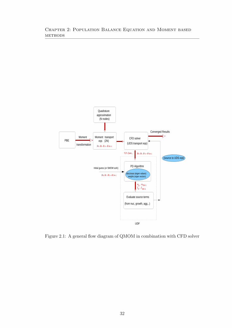
Chapter 2: Population Balance Equation and Moment basedmethods
PBE
PD Algorithm
weights (eigen vectors)abscissas (eigen values)
10 2N−1µ , µ , µ ....µ2
10 2N−1µ , µ , µ ....µ2
Quadrature
(N nodes)approximation
10 2N−1µ , µ , µ ....µ2
Initial guess (or SMOM soln)
Evaluate source terms
Converged Results
CFD solver
UDF
(2N)Moment transport
eqsMoment
transformation
(from nuc, growth, agg...)
(source to UDS eqs)
0
0 2N−1
2N−1w ... wξ ... ξ
T,P, Conc...
(UDS transport eqs)
Figure 2.1: A general flow diagram of QMOM in combination with CFD solver
32

Chapter 2: Population Balance Equation and Moment basedmethods
Step 3 Generate the α vector from the elements of P matrix (see Eq. 2.22):
α(1) = 0 (2.21)
α(i) =P (1, i+ 1)
[P (1, i)P (1, i− 2)]∀i ≥ 2 (2.22)
Step 4 Evaluate the diagonal a1, a2...(a2N ) and off-diagonal elements b1,
b2...(b2N−1) from the α vector, see Eq. (2.24):
a(i) = α(2i) + α(2i− 1) (2.23)
[b(i)]2 = α(2i+ 1)α(2i) (2.24)
Step 5 Construct the Jacobi matrix (J) from the diagonal and the co-diagonal
elements. Please note that the order of the Jacobi matrix would be
equal to the number of quadrature nodes N . Now, this Jacobi matrix
is tridiagonal and symmetric, hence all the eigenvalues are real. This
completes the PD algorithm.
J =
a1 b1 0
b1 a2 b2
0 b2 a3
Step 6 Find out the eigenvalues (λ) and eigenvectors (ν) of this Jacobi ma-
trix.
Step 7 The eigenvalues are directly the abscissas of the quadrature approxi-
mation, and the eigenvectors give the weights of the quadrature approx-
imation, see Eq. (2.26).
ξ(i) = λi (2.25)
w(i) = µ0ν2i1 (2.26)
Step 8 Evaluate the source terms for the moment transport equations.
33

Chapter 2: Population Balance Equation and Moment basedmethods
Step 9 Push these source terms into CFD solver as the source terms to UDS
transport equations.
Step 10 With the CFD solver, evaluate the new set of moments.
Step 11 Repeat the Step 2 to Step 10 till the solution converges.
2.4 Solution of population balance equations
using DQMOM
The Direct Quadrature Method of Moments (direct QMOM or DQMOM) is
conceptually similar to QMOM, but the solver formulation is different. Solving
the moment transport equations in QMOM is similar to that of SMOM, but
the weights and abscissas are obtained from the PD algorithm. DQMOM does
not solve for the moments, instead, it solves directly the variables appearing in
the Quadrature approximation i.e., the weights and abscissas. Thus, DQMOM
does not use the PD algorithm. Therefore, in DQMOM, the weights and
the abscissas are transported in the computational domain with their own
velocities. Thus, it leads to a strong coupling between internal co-ordinates
and phase velocities.
Pioneering research work on DQMOM has been done by Marchisio and
Fox [49], with a clear mathematical description and applications to various
industrial problems including combustion, fluidized beds, precipitation, etc.
[30, 81, 88, 107]. There are two main reasons for choosing DQMOM over
QMOM, as discussed by authors. When the internal co-ordinates are inte-
grated out to transform the PBE into its moment equations (as in QMOM),
the strong coupling between the internal co-ordinates and the phase velocities
is not accounted for in QMOM, while in DQMOM this coupling is retained.
Secondly, the extension of QMOM to bivariate or higher PBE is quite cumber-
some when NDF (f) depends on two or more internal co-ordinates [87, 111].
The main difficulty in this case is the lack of efficient numerical algorithms to
invert the moments into wi and ξi, like PD algorithm. Instead, DQMOM solves
the transport equations of wi and ξi directly in the domain and thus lowers
the computational costs drastically. However, it now appears that DQMOM
34
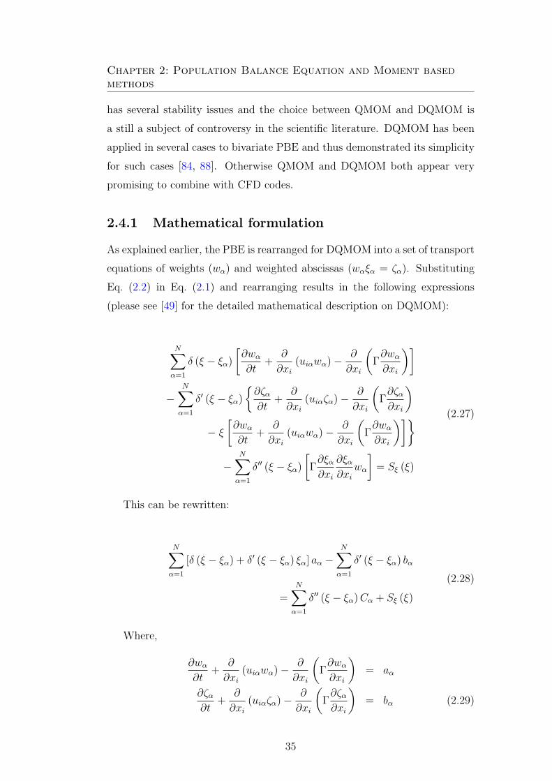
Chapter 2: Population Balance Equation and Moment basedmethods
has several stability issues and the choice between QMOM and DQMOM is
a still a subject of controversy in the scientific literature. DQMOM has been
applied in several cases to bivariate PBE and thus demonstrated its simplicity
for such cases [84, 88]. Otherwise QMOM and DQMOM both appear very
promising to combine with CFD codes.
2.4.1 Mathematical formulation
As explained earlier, the PBE is rearranged for DQMOM into a set of transport
equations of weights (wα) and weighted abscissas (wαξα = ζα). Substituting
Eq. (2.2) in Eq. (2.1) and rearranging results in the following expressions
(please see [49] for the detailed mathematical description on DQMOM):
N∑
α=1
δ (ξ − ξα)
[∂wα
∂t+
∂
∂xi
(uiαwα)−∂
∂xi
(Γ∂wα
∂xi
)]
−
N∑
α=1
δ′ (ξ − ξα)
{∂ζα∂t
+∂
∂xi
(uiαζα)−∂
∂xi
(Γ∂ζα∂xi
)
− ξ
[∂wα
∂t+
∂
∂xi
(uiαwα)−∂
∂xi
(Γ∂wα
∂xi
)]}
−N∑
α=1
δ′′ (ξ − ξα)
[Γ∂ξα∂xi
∂ξα∂xi
wα
]= Sξ (ξ)
(2.27)
This can be rewritten:
N∑
α=1
[δ (ξ − ξα) + δ′ (ξ − ξα) ξα] aα −
N∑
α=1
δ′ (ξ − ξα) bα
=N∑
α=1
δ′′ (ξ − ξα)Cα + Sξ (ξ)
(2.28)
Where,
∂wα
∂t+
∂
∂xi
(uiαwα)−∂
∂xi
(Γ∂wα
∂xi
)= aα
∂ζα∂t
+∂
∂xi
(uiαζα)−∂
∂xi
(Γ∂ζα∂xi
)= bα (2.29)
35
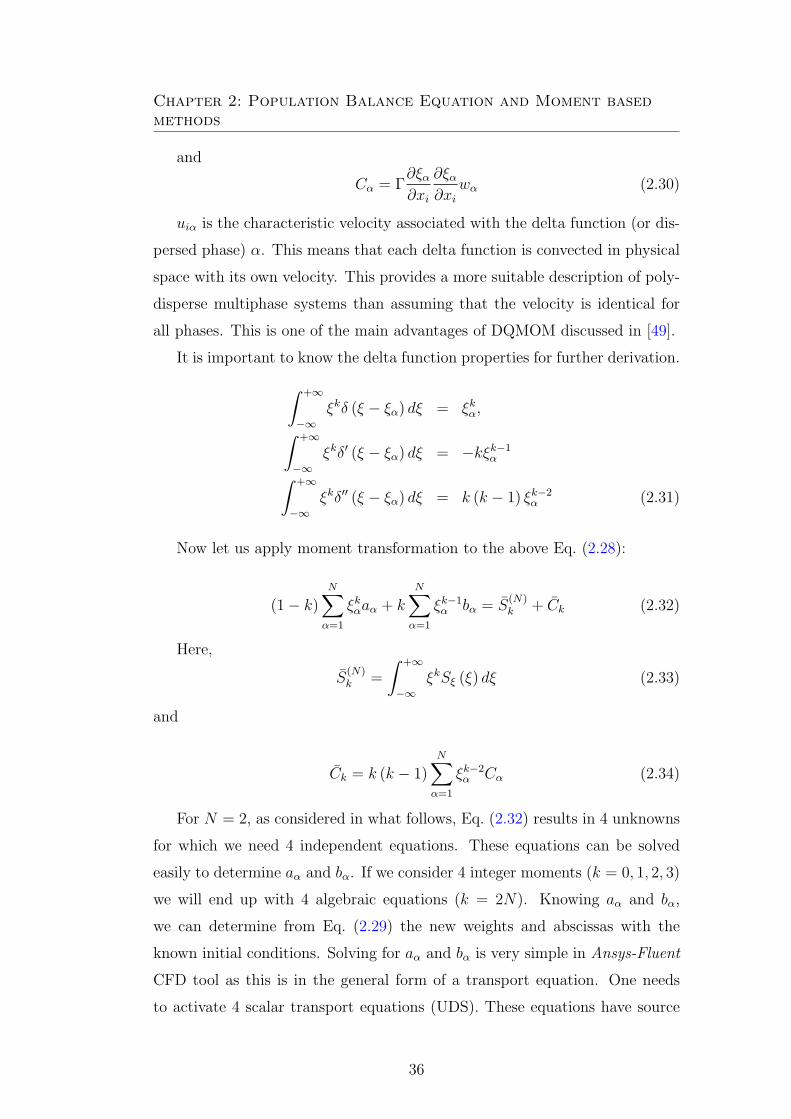
Chapter 2: Population Balance Equation and Moment basedmethods
and
Cα = Γ∂ξα∂xi
∂ξα∂xi
wα (2.30)
uiα is the characteristic velocity associated with the delta function (or dis-
persed phase) α. This means that each delta function is convected in physical
space with its own velocity. This provides a more suitable description of poly-
disperse multiphase systems than assuming that the velocity is identical for
all phases. This is one of the main advantages of DQMOM discussed in [49].
It is important to know the delta function properties for further derivation.
∫ +∞
−∞
ξkδ (ξ − ξα) dξ = ξkα,
∫ +∞
−∞
ξkδ′ (ξ − ξα) dξ = −kξk−1α
∫ +∞
−∞
ξkδ′′ (ξ − ξα) dξ = k (k − 1) ξk−2α (2.31)
Now let us apply moment transformation to the above Eq. (2.28):
(1− k)N∑
α=1
ξkαaα + k
N∑
α=1
ξk−1α bα = S
(N)k + Ck (2.32)
Here,
S(N)k =
∫ +∞
−∞
ξkSξ (ξ) dξ (2.33)
and
Ck = k (k − 1)N∑
α=1
ξk−2α Cα (2.34)
For N = 2, as considered in what follows, Eq. (2.32) results in 4 unknowns
for which we need 4 independent equations. These equations can be solved
easily to determine aα and bα. If we consider 4 integer moments (k = 0, 1, 2, 3)
we will end up with 4 algebraic equations (k = 2N). Knowing aα and bα,
we can determine from Eq. (2.29) the new weights and abscissas with the
known initial conditions. Solving for aα and bα is very simple in Ansys-Fluent
CFD tool as this is in the general form of a transport equation. One needs
to activate 4 scalar transport equations (UDS). These equations have source
36
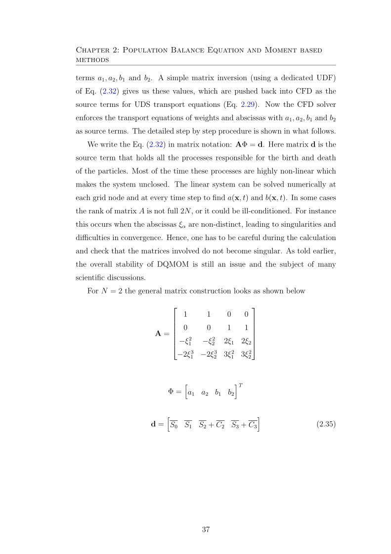
Chapter 2: Population Balance Equation and Moment basedmethods
terms a1, a2, b1 and b2. A simple matrix inversion (using a dedicated UDF)
of Eq. (2.32) gives us these values, which are pushed back into CFD as the
source terms for UDS transport equations (Eq. 2.29). Now the CFD solver
enforces the transport equations of weights and abscissas with a1, a2, b1 and b2
as source terms. The detailed step by step procedure is shown in what follows.
We write the Eq. (2.32) in matrix notation: AΦ = d. Here matrix d is the
source term that holds all the processes responsible for the birth and death
of the particles. Most of the time these processes are highly non-linear which
makes the system unclosed. The linear system can be solved numerically at
each grid node and at every time step to find a(x, t) and b(x, t). In some cases
the rank of matrix A is not full 2N , or it could be ill-conditioned. For instance
this occurs when the abscissas ξα are non-distinct, leading to singularities and
difficulties in convergence. Hence, one has to be careful during the calculation
and check that the matrices involved do not become singular. As told earlier,
the overall stability of DQMOM is still an issue and the subject of many
scientific discussions.
For N = 2 the general matrix construction looks as shown below
A =
1 1 0 0
0 0 1 1
−ξ21 −ξ22 2ξ1 2ξ2
−2ξ31 −2ξ32 3ξ21 3ξ22
Φ =[a1 a2 b1 b2
]T
d =[S0 S1 S2 + C2 S3 + C3
](2.35)
37
Chapter 2: Population Balance Equation and Moment basedmethods
2.4.2 Source terms evaluation for the different processes
In the case of DQMOM the source terms are all similar to that employed for
QMOM. The interested reader should look back at Section 2.3.2.
2.4.3 Steps involved in DQMOM
Figure 2.2 is the general solution procedure used for the solution of DQMOM
in combination with CFD solver. The sequence of steps used in DQMOM is
explained below.
Step 1 Formulate the PBE into set of transport equations of weights and
weighted abscissas (see Eq. 2.29) by rearranging and using moment trans-
formation.
Step 2 Evaluate the source terms (see Eq. 2.33), start first with an initial
guess/SMOM solution.
Step 3 Solve the system of equations using any efficient matrix inversion al-
gorithm (by using a UDF) to obtain a1, a2, ...b1, b2.... (see Eq. 2.32).
Step 4 Push these values into CFD-solver, as these are the source terms for
the user defined scalar transport equations (UDS, see Eq. 2.29).
Step 5 Using these values CFD-solver gives new set of weights and weighted
abscissas in the next iteration.
Step 6 Repeat from Step 2 to Step 5 till the solution converges.
2.5 Numerical results with QMOM/DQMOM
Certainly, the number of quadrature nodes determines to some extent the accu-
racy of the solution. Published results from the literature show that quadrature
methods with 2 or 3 nodes are usually sufficient to obtain the most important
moments with the desired accuracy [107]. Of course, increasing the number of
nodes leads in principle to improved predictions, but also to a rapid increase
in computational time.
38

Chapter 2: Population Balance Equation and Moment basedmethods
Quadrature
(N nodes)approximation
(Source to UDS eqs)
Transport eqs (2N)
0ζ ....ζ2N−1
0w ...w 2N−1
0ζ ....ζ2N−1
0w ...w 2N−1
0ζ ....ζ2N−1
0w ...w 2N−1
CFD Solver
PBE
Evaluate source termsnuc, growth, agg ...
Solve for a1, a2... b1, b2 ...
a1, a2... b1, b2 ...
T, P, Conc....
UDF
Rearrange &
transformation
Moment−
Initial guess (or SMOM soln)
Converged Results
(eqs)(UDS transport −)
Figure 2.2: A general flow diagram of DQMOM in combination with CFDsolver
39

Chapter 2: Population Balance Equation and Moment basedmethods
The following discussion is solely aimed at understanding QMOM/DQMOM
in dealing with the particulate problems considered here. The results are eval-
uated for few test problems and the modeling details are not discussed now,
they will be given in later Chapters. The emphasis in the following results is
only on the application of QMOM/DQMOM in describing nanoparticle (soot,
TiO2) evolution in typical flame configurations.
Figure 2.3 shows the first 4 moments of the NDF (f) of soot particles
along the axis of a turbulent ethylene/air diffusion flame. Nucleation, molecu-
lar growth, oxidation and aggregation have been considered in the calculations.
The calculations are performed with N = 2 nodes for QMOM and DQMOM,
N = 3 nodes with QMOM. As seen in these figures the QMOM and DQ-
MOM predicted the same behaviour and the results are almost identical for
the first moments (µ0, µ1). As explained earlier both methods only differ in the
implementation and should yield in principle identical results for uni-variate
problem. However, a small difference is noticed in the moments predicted by
both methods, becoming more visible for higher moments like µ3. This is
due to the differences in the numerical methods employed. The issue becomes
more serious for higher moments due to bad conditioning. The dotted line in
the figure is evaluated with 3 quadrature nodes. The results obtained with 3
nodes for this configuration do not differ very much from those obtained with
2 quadrature nodes, confirming statements from the literature. The relative
difference for the only important quantities µ0, µ1 and µ3 (almost identical,
hence the curves are overlapped) is below 1%, and hence finally acceptable for
practicle applications. Therefore, 2 nodes have been retained throughout this
project in order to speed-up corresponding computations.
Figure 2.4 shows the contour plots of the first 4 moments of soot NDF
obtained with QMOM and DQMOM for the flame configuration of [52]. The
PBE is represented here with 2 quadrature nodes and particle length as internal
co-ordinate. As seen in these figures, the predictions are almost identical with
QMOM and DQMOM in qualitative as well as in quantitative behavior, with
relative differences in peak values below 4% for the first moments.
Due to higher stability, QMOM has been also successfully implemented in
the present study to predict TiO2 nanoparticle evolution in turbulent CH4/O2/Ar/TTIP
40

Chapter 2: Population Balance Equation and Moment basedmethods
0 0.1 0.2 0.3 0.4 0.5 0.6 0.7Axial position (m)
0
5e+15
1e+16
1.5e+16
2e+16
2.5e+16
µ 0
DQMOM with 2 nodes
QMOM with 2 nodes
QMOM with 3 nodes
0 0.1 0.2 0.3 0.4 0.5 0.6 0.7Axial position (m)
0
1e+08
2e+08
3e+08
4e+08
5e+08
6e+08
µ 1
DQMOM with 2 nodes
QMOM with 2 nodesQMOM with 3 nodes
0 0.1 0.2 0.3 0.4 0.5 0.6 0.7Axial position (m)
0
5
10
15
20
25
30
µ 2
DQMOM with 2 nodes
QMOM with 2 nodes
QMOM with 3 nodes
0 0.1 0.2 0.3 0.4 0.5 0.6 0.7Axial position (m)
0
5e-07
1e-06
1.5e-06
2e-06
2.5e-06
3e-06
µ 3
DQMOM with 2 nodes
QMOM with 2 nodes
QMOM with 3 nodes
Figure 2.3: Comparison of moments of the NDF obtained withQMOM/DQMOM for the soot particle formation in turbulent ethylene/airflame [52]. Note the highly different y-scales. For µ3 using 2 and 3 nodes theresults are almost identical with QMOM, hence the curves are overlapped.
41

Chapter 2: Population Balance Equation and Moment basedmethods
������������������������������������������������������������������������������������������������������������������������������
������������������������������������������������������������������������������������������������������������������������������
��������������������������������������������������������������������������������������������������������
��������������������������������������������������������������������������������������������������������
QMOM DQMOM
Figure 2.4: Contour plots of first 4 moments (from top µ0 in 1/m3, µ1 in m/m3,µ2 in m2/m3, µ3 in ppm) of soot PSD obtained with QMOM and DQMOMfor turbulent ethylene/air flame configuration of [52]
42

Chapter 2: Population Balance Equation and Moment basedmethods
diffusion flame. In this case QMOM with 2 quadrature nodes has been con-
sidered and the source term includes nucleation, molecular growth and aggre-
gation.
43
Chapter 3
Employed numerical models
The present chapter discusses the computational models used in various stages
of this research work. As the investigations here involve particle phase and
gas-phase simultaneously, the models are classified into two main groups called
‘gas-phase models’ and ‘particle phase models’.
The governing equations and the models used in the present study are de-
picted in Fig. 3.1. The industrial CFD solver Ansys-Fluent is employed to solve
all the gas-phase transport equations. Ansys-Fluent is a finite-volume based
numerical solver and solves here the so-called Favre-averaged Navier-Stokes
equations. The evolution of the particle phase is represented with popula-
tion balance equations (PBE) solved with moment based methods (QMOM /
DQMOM), as described in the previous chapter.
3.1 Gas phase models
3.1.1 Computational Fluid Dynamics (CFD)
Computational fluid dynamics (CFD) provides solution for a wide range of
engineering problems by solving governing mathematical equations such as
conservation of mass, momentum, energy, species, etc., which describe the
given system. In turbulent flows all the flow properties vary in a random and
chaotic way. Direct numerical simulation (DNS) is limited to very simplified
cases, where the time and length scales present in the system are small. One
way of handling this is to solve for the mean flow field by averaging the balance
44
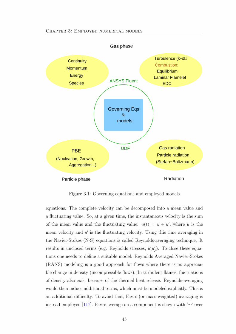
Chapter 3: Employed numerical models
RadiationParticle phase
Gas phase
Continuity
Energy
Species
Momentum
Aggregation...)
(Nucleation, Growth,
Governing Eqs
models
Gas radiation
Particle radiation
(Stefan−Boltzmann)
&
Turbulence (k−ε)
EDC
Laminar Flamelet
Equilibrium
PBE
ANSYS Fluent
UDF
Combustion:
Figure 3.1: Governing equations and employed models
equations. The complete velocity can be decomposed into a mean value and
a fluctuating value. So, at a given time, the instantaneous velocity is the sum
of the mean value and the fluctuating value: u(t) = u + u′, where u is the
mean velocity and u′ is the fluctuating velocity. Using this time averaging in
the Navier-Stokes (N-S) equations is called Reynolds-averaging technique. It
results in unclosed terms (e.g. Reynolds stresses, u′
iu′
j). To close these equa-
tions one needs to define a suitable model. Reynolds Averaged Navier-Stokes
(RANS) modeling is a good approach for flows where there is no apprecia-
ble change in density (incompressible flows). In turbulent flames, fluctuations
of density also exist because of the thermal heat release. Reynolds-averaging
would then induce additional terms, which must be modeled explicitly. This is
an additional difficulty. To avoid that, Favre (or mass-weighted) averaging is
instead employed [117]. Favre average on a component is shown with ‘∼’ over
45

Chapter 3: Employed numerical models
it : u(t) = u + u′′, and u = ρuρ. This averaging results in similar equations to
that appearing in Reynolds-averaging of incompressible flows. The unclosed
Reynolds stresses are similarly closed with appropriate turbulence models. The
simplified Favre-averaged balance equations for the present problem are shown
below.
Continuity equation :∂ρ
∂t+
∂ρui
∂xi
= 0 (3.1)
Momentum equation :
∂ρui
∂t+
∂ρuiuj
∂xi
= −∂p
∂xi
+ (ν + νt)∂2ρui
∂xj∂xj
+∂ρu′′
i u′′
j
∂xi
+ ρg (3.2)
Scalar transport equation for the αth component :
∂ρφα
∂t+
∂ρφαui
∂xi
= (Γ + Γt)∂2ρφα
∂xi∂xi
+∂ρφ′′
αu′′
i
∂xi
+ S (φ) (3.3)
Energy equation in terms of total enthalpy ht, with ht = h+ uiui
2:
∂ρht
∂t+
∂ρhtui
∂xi
=∂p
∂t−
∂ρu′′
i h′′
t
∂xi
+∂
∂xi
(J h
i + uiτji
)+ uiFi + S (h) (3.4)
where ρ and p are the mean density and pressure, respectively, ui is the Favre-
averaged value of the ith component of the fluid mean velocity, u′′
i is the
ith component fluctuation velocity. φ and φ′′ are the mean and fluctuating
concentration of the αth scalar, ν, νt are kinematic and turbulent viscosities
respectively; Γ,Γt are molecular and turbulent diffusivities respectively; S (φ)
is Favre-averaged chemical source term, ht is Favre-averaged total enthalpy, h′′
t
is its fluctuating component, J hi is averaged enthalpy diffusive flux, uiτji and
uiFi denote respectively the averaged power due to viscous and body forces,
S (h) is Favre-averaged heat source. In the present case this source is due to
radiative heat transfer, is evaluated through a User Defined Function (UDF)
and provided as a source term to energy transport equation in Ansys-Fluent.
Repeated indices imply summation.
The Reynolds stresses in Eq. (3.2) are closed by k − ǫ turbulence model.
The simplest models for turbulent flows are those based on the concept of tur-
46

Chapter 3: Employed numerical models
bulent viscosity (µt) and turbulent diffusivity (Γt). We have always used k− ǫ
turbulence model, one of several available models from the literature. This
model is very simple, very widely used, requires moderate computational time
and has been successfully validated for the present flow problem (non-swirling
jet flows) [118]. According to this model, Γt is evaluated from turbulent kine-
matic viscosity (νt).
νt = Cµk2
ǫ(3.5)
Here, Cµ = 0.09, k, ǫ are turbulent kinetic energy and turbulent dissipation
rate respectively, and Γt = νtSct
, where Sct is the turbulent Schmidt number
(ratio of momentum diffusivity to mass diffusivity, νtΓt
), assumed equal to 0.7
as usual.
3.1.2 Non-premixed turbulent combustion
In non-premixed combustion fuel and oxidizer are not mixed a priory. Instead
they enter seperately into combustion zone. Later, the mixing takes place due
to convection, turbulent and molecular interdiffusion. Since diffusion is the
rate-controlling process, this configuration is often known as diffusive com-
bustion and the corresponding flames are known as diffusion flames. Since
the time needed for turbulent mixing (τφ) is typically much larger than the
time needed for combustion (τα) the assumption of infinitely fast chemistry (or
local chemical equilibrium) usually appears to be appropriate. This assump-
tion introduces an important simplication in modeling turbulent non-premixed
flames [119], as detailed in later sections.
In the present work, first studies of soot production in turbulent/ethylene
flames use equilibrium chemistry approximation. In later cases, a considerably
refined description of gas-phase chemistry has been achieved by employing
laminar flamelet modeling and describing chemical kinetics with 36 species
and 219 chemical reactions [120]. Then turbulence and chemistry interactions
are modeled through presumed PDF approach. For single mixture fraction
cases, Ansys-Fluent uses an assumed shape β-function, since it accurately
represents experimentally observed PDFs of mixture fraction.
47

Chapter 3: Employed numerical models
When modeling later TiO2 particles in CH4-O2-Ar diffusion flames, Eddy
Dissipation Concept (EDC) model has been applied. In the following sections,
a short description of these combustion models are given.
3.1.3 Gas phase chemistry
Due to the complexity of turbulent flows and chemical kinetics, as well as
their interaction, it is extremely difficult to obtain direct numerical solutions by
DNS. Consequently the interaction between turbulence and chemistry must be
usually modeled [121]. In turbulent combustion modeling, the chemical source
term is the main closure difficulty. Good amount of research has been done
and is still going on to develop better models for this closure. Approximate
closure depends on range of chemical (τα) and turbulent (τφ) time scales. It
is proved in the literature that, in the equilibrium-chemistry limit an accurate
closure can be developed by using the mixture fraction (Z) PDF. Mixture
fraction is the scaled mass fraction of unburnt fuel (C, H) in the local mixture
with Z = 1 in pure fuel and Z = 0 in pure oxidizer. The problem can be
greatly simplified when we reformulate the problem in terms of the mixture
fraction (Z) under the assumption of equilibrium-chemistry limit. Here, it
is assumed that all the chemical species reach their equilibrium values much
faster than the characteristic time scales of flow, i.e τα ≪ τφ (large Damkholer
number, Da=τφτα). One additional assumption made in the derivation is that
the molecular diffusion coefficients are equal for all species. This assumption
results in a unique mixture fraction definition. Thus, under these assumptions
the reacting scalars can be represented through the mixture fraction. The
only PDE that must be solved is that of the mixture fraction. Please note
that mixture fraction is a conserved scalar quantity, therefore its governing
equation does not have any chemical source term in it [117, 122].
The Favre-averaged mixture fraction transport equation is shown below:
∂(ρZ)
∂t+ ui
∂(ρZ)
∂xi
= (Γ + Γt)∂2(ρZ)
∂xixi
(3.6)
Now the numerical simulation of turbulent combustion is greatly simplified
to a simple mixing problem and the difficulties associated with closing non-
48
Chapter 3: Employed numerical models
linear mean reaction rates are avoided. Temperature, composition and density
will be calculated at different points knowing mixture fraction PDF. Since the
mixture fraction PDF is not known a priory, it must be modeled by solving
an appropriate transport equation or by assuming a functional form. The
most widely used approach is the presumed PDF method, in which a known
distribution function is chosen to represent the mixture fraction PDF. For a
one-component mixture fraction vector a β-PDF is often employed. A chemical
look-up table is created and the mean values of temperature, mole fraction and
density are saved at different values of mixture fraction in this table. This is
the common solution procedure for both the equillibrium combustion model
and the laminar flamelet combustion model.
3.1.4 Equilibrium combustion model
When we assume that chemical reactions are infinitely fast (‘mixed is burnt’)
then the equilibrium combustion model can be used. In this case all the species
tranport equations can be reduced to transport a single equation of mixture
fraction (Z).
As already explained previously, the emphasis of the present work is not
set on the extremely difficult issue of gas-phase or surface kinetics. Therefore,
gas-phase chemistry is described very simply in first simulations by using a
mixture fraction approach with equilibrium chemistry approximation, while
turbulence/chemistry interactions are modeled through a presumed β-PDF
approach, solving transport equations for mixture fraction Z and for its vari-
ance Z ′′2 [117]. Twenty chemical species (C2H4, O2, H2, CO, CH4, CO2, H2O,
C2H2, OH, H, O, C6H6, C4H2, C2N2, C4H, C3H2, H2CCCCH, C2H6, C2N, N2)
are taken into account in the equilibrium calculation.
During this study, it appeared that equilibrium chemistry was sometimes
insufficiently accurate. Further improvement in the gas-phase chemistry was
achieved through laminar flamelet modeling. The main advantage of the
flamelet approach is that it takes into account finite-rate kinetic effects.
49

Chapter 3: Employed numerical models
3.1.5 Laminar flamelet combustion model
When the chemical reactions are fast (Da > 1), but not infinitely fast (Da
≫ 1) the laminar flamelet approach is used instead. The laminar flamelet
approach is based on a representation of a turbulent flame as an ensemble of
streched laminar flame elements embeded in a turbulent flow and interacting
with it. This model may be viewed as a direct improvement of the infinitely
fast chemistry model, since it uses the same formalism, but with an addi-
tional parameter, the scalar dissipation rate (χ), thereby including finite rate
chemistry effects [117]. Laminar flamelet combustion models allow to include
detailed chemical mechanism and finite rate effects. A flamelet table must first
be generated.
One key parameter of the flamelet structure is the scalar dissipation rate
χ (see Eq. 3.7), which controls the reactant fluxes to the reaction zone and is
related to the flow velocity gradients.
χ = 2Γ|∇Z|2 (3.7)
In Ansys-Fluent the turbulence-chemistry interactions are modelled with a
presumed β-PDF. The advantage of the flamelet combustion model is that it
is still computationally efficient as it solves only two tranport equations (mean
mixture fraction and its variance), but simultaneously incorporates finite-rate
chemistry.
We have systamatically employed 10 flamelet profiles into the flamelet look-
up table for all calculations employing laminar flamelet modeling in the present
study.
3.1.6 Eddy Dissipation Concept Model (EDC)
Magnussen first developed the Eddy Dissipation Concept Model (EDC) for
describing chemical reations in a turbulent flow. The turbulence energy cas-
cade model is the basis for EDC. The model is developed on the fact that the
molecular mixing between reactants, which is associated with the turbulence
dissipation ǫ, takes place in concentrated, isolated regions (dissipative) that
occupy only a small fraction of the total volume of the fluid [121]. Within these
50
Chapter 3: Employed numerical models
small-scale regions, small-scale structures are found whose dimension is of the
same magnitude as the Kolmogorov microscale. Within these structures, one
can assume that the reactants are mixed homogeneously at molecular level.
These structures thus create the reaction space for non-uniformly distributed
reactants and now act as a well-mixed reactor. In this case, chemical reaction
kinetics determine the speed of the process. Outside these small scales the
reactants are not mixed and hence do not react. Therefore, in order to be
able to treat these reactions within this space it is necessary to know the re-
action volume and the mass transfer rate between the fine structures and the
surrounding fluid. These dissipative regions and the mass transfer rates into
surrounding fluid are solely determined by turbulence theory, thus enabling
fast and accurate calculations of turbulent reactive flows, in particular turbu-
lent combustion. Now, each reactive cell is split into reactive volume fraction
(γ3) and an inert fraction (1− γ3). The volume fraction of the reactive portion
is modelled as [123, 124]:
γ3 = Cγ
(νǫk2
)3/4
(3.8)
where, Cγ is volume fraction constant and it is evaluated using model constants
CD1 = 0.134 and CD2 = 0.5 as:
Cγ =
(3CD2
4C2D1
)1/4
= 2.1377 (3.9)
The time scale for the mass transfer (τ) from the small-scale structures to the
surrounding fluid is [123, 124] :
τ = Cτ
(νǫ
)1/2
(3.10)
where, Cτ is a time scale constant which is equal to:
Cτ =
(CD2
3
)1/2
= 0.4083 (3.11)
The advantage of the EDC model is that it can incorporate some amount
of detailed chemistry and both fast and slow chemical reactions can be treated
simultaneously allowing to describe extinction [125].
51

Chapter 3: Employed numerical models
In order to make detailed chemistry calculations more efficiently Ansys-
Fluent uses In Situ Adaptive Tabulation (ISAT). ISAT can accelerate the
chemistry calculations by up to 2 − 3 orders of magnitude [124], thereby re-
ducing the computational time. The fine scales are represented as isobaric,
perfectly stirred reactors in Ansys-Fluent.
However, it is shown in Chapter 6 that the default EDC model parameters
over predicted the temperature field for the considered configurations. There-
fore, a parameter analysis has been carried out to find better values. For all
later simulations EDC parameters are finally taken as Cγ = 2.1377 (standard
value) and Cτ = 3.4.
In the following section particle phase models employed for modeling soot
and TiO2 are described.
3.2 Dispersed phase chemical and physical mod-
els
The detailed literature analysis of Chapter 1 shows that, the main processes
are nucleation, surface growth, aggregation and possibly oxidation.
3.2.1 Particle phase models : Soot
As explained previously, the model combination proposed and validated in
[30] has been retained as original model combination for initial predictions
and as starting point for the optimization. As a consequence, the nucleation
model introduced in [126] and the molecular growth model presented in [127]
have been retained, both acetylene-based. Oxidation results only from O2
molecules, as proposed in [38].
52
Chapter 3: Employed numerical models
3.2.1.1 Nucleation, Growth and Oxidation rates
The rates of nucleation J , molecular growth Gg and oxidation Go are finally
written:
J = NAρ2T
1
26 106 exp
(−Tn
T
)XC2H2
(3.12)
Gg =6
Dfρs
(Rc
Rc0
) 3−Df
3
2 Ms 6 exp
(−Tg
T
)[C2H2] (3.13)
Go =p
DfρsT−
1
26.5 exp
(−To
T
)YO2
(3.14)
Here, X is mole fraction, Y is mass fraction, Ms = 12 g/mol is soot molecular
weight, NA is Avogadro’s number, [C2H2] represents the acetylene concentra-
tion. The parameters Tn, Tg and To are equivalent activation temperatures for
nucleation, growth and oxidation, respectively.
The aggregation kernel β12, which depends on the Knudsen number, Kn =
2λL
(the ratio between the molecular mean free path of gas molecules, λ and
the particle radius, L/2) is evaluated by the Fuchs interpolation formula [30]:
β12 = 4π(D1 +D2)(Rc1 +Rc2)
[Rc1 +Rc2
Rc1 +Rc2 + (g21 + g22)1
2
+
4(D1 +D2)
Rc1 +Rc2 + (c21 + c22)1
2
]−1 (3.15)
where,
ci =
√8kbT
πmi
Di =kbT
6πµRci
[5 + 4Kni + 6Kn2
i + 18Kn3i
5−Kni + (8 + π)Kn2i
]
li =8Di
πci
gi =(2Rci + li)
3 − (4R2ci + l2i )
3
2
6Rcili− 2Rci
with m the particle mass and kb the Boltzmann constant. The parameter Rc
is the collision radius, which is defined in terms of the fractal dimension Df of
53
Chapter 3: Employed numerical models
the aggregate through
Rc = kfL0
2
(V
V0
) 1
Df
(3.16)
with V the aggregate volume. The subscript 0 indicates primary particles, as-
sumed of size 15 nm, and kf is the fractal prefactor of order unity. The present
simulation results are mostly computed by considering a constant fractal di-
mension Df = 1.8 and kf = 1, since a sensitivity analysis as described later
revealed that the predicted soot volume fraction (fv) is not very sensitive
against Df .
In order to check this issue, fractal dimension Df has been evaluated as
described below for some cases. The evolution of the mean value of the fractal
dimension is calculated as a function of characteristic fusion time (tf , some-
times referred as characteristic restructuring time) and collision time (tc) and
changes its value during particle growth, aggregation, etc. Here, a character-
istic number τ is defined, which can be correlated with Df [128]:
τ =tctf
(3.17)
The characteristic time tc is determined by following approach, explained
in [128]:
tc =1
βm0
(3.18)
where, β is the aggregation kernel calculated with average particle diameter
(mean aggregation kernel), m0 is the number concentration of the particles
(i.e, zeroth moment, m0 = µ0).
The characteristic fusion/restructuring time tf can be assumed for soot
particles [30] as:
tf =
√15νtǫ
(3.19)
Here, νt is turbulent kinematic viscosity and ǫ is turbulent dissipation rate.
For different values of τ , Df is modelled as [128]:
Df =
Df,min + (Df,0 −Df,max)
1/τs τ ≤ 1,
Df,max − (Df,max −Df,0)τs τ > 1,
(3.20)
54
Chapter 3: Employed numerical models
If tf is much smaller than tc, adherent particles will nearly always be com-
pletely fused prior to the next collision event. Therefore, mostly isolated spher-
ical particles will be formed with a fractal dimension Df = Df,max = 3. In
the opposite case, thus if tc is much smaller than tf , adherent particles will
face their next collision event far before sintering has been terminated. Ag-
glomerates with fractal dimensions around Df = Df,min = 1.8 as common for
cluster-cluster aggregation will be generated then.
Here, s is a parameter which determines the gradient of the above function,
Df,0 = Df (τ = 1) accounts for the fractal dimension at identical characteristic
collision and fusion time and is assumed to be equal to the average value
between the limiting cases (Df,min and Df,max), thus equal to 2.4.
It has been shown later in the results that inclusion of variable fractal
dimension does not play any noticeable role for the soot volume fraction (fv)
value, the most important quantity for our investigation. Therefore, it has
been fixed to a value of 2.0 for all further calculations.
3.2.2 Particle phase models : TiO2
The last part of the present study deals with the synthesis of TiO2 nanopar-
ticles from titanium tetraisopropoxide in CH4-O2 diffusion flames with Ar as
precursor. TiO2 nanoparticle evolution is represented by taking into account
nucleation, growth and aggregation as the source terms. The detailed analy-
sis of literature shows that there is a serious dearth of computational models
for evaluating essential parameters and reaction rates. Nevertheless, following
rate equations appear to be commonly accepted. Certainly, more and better
experimental measurements are needed in the future.
3.2.2.1 Overall rate:
The overall thermal decomposition of titanium tetraisopropaxide (Ti(OCH(CH3)2)4)
occurs both by homogeneous gas phase reaction and on the surface of TiO2
particles.
dCTTIP
dt= −kov = − (kg + ksA)CTTIP (3.21)
55
Chapter 3: Employed numerical models
where, CTTIP is concentration (in mol/m3) of titanium tetraisopropaxide (TTIP).
A is the particle area concetration (m2/m3). kov, kg and ks are the rate con-
stants of overall TTIP decomposition, nucleation and surface growth respec-
tively. The underlying, global reaction reads:
TTIP −→ TiO2 + 4 C3H6 + 2 H2O
The overall reaction rate constant kov (1/s), derived from experimental
data as in [129] is:
kov = 3.96 105exp
(−8479.7
T
)for T = 500− 670 K (3.22)
3.2.2.2 Growth rate:
The surface reaction rate constant ks (m/s) is obtained from [130]:
ks = 109exp
(−15155
T
)for T = 660− 700 K (3.23)
3.2.2.3 Nucleation rate:
Knowing the overall decomposition rate of TTIP (kov) and the corresponding
surface contribution (ks), the nucleation rate (kg in 1/s) is obtained through
the following expression.
kg = kov − Aks (3.24)
When the surface reaction rate is neglected, ks=0 and kg = k. Since both
rates have been modeled completely independently, it happens that the surface
reaction rate ks (Eq. 3.23) becomes larger than the overall rate kov, (Eq. 3.22),
which is obviously non-physical. In this case, the surface reaction rate is simply
prescribed as ks = kov/A and kg = 0, so that the mass balance is correctly
preserved, following corresponding recommendations from the literature [80].
3.2.2.4 Expressions for nucleation, growth and aggregation
The rate of nucleation (J , #/m3) and molecular growth (G, m3/s) are [59]:
56
Chapter 3: Employed numerical models
J = NA kg CTTIP (3.25)
G = ks CTTIP Ag NA vp0 (3.26)
where, NA, Ag, vp0 are the Avagadro’s number, mean particle surface area
and initial volume of the titania monomer, respectively.
The employed brownian aggregation kernel β(v1, v2) of particles of volume
(v1 and v2) is:
β(v1, v2) =
(3
4π
)1/6 (6kBT
ρp
)1/2 (1
v1+
1
v2
)1/2
×(v1/31 + v
1/32
)2
(3.27)
3.2.3 Heat of reaction of TTIP decomposition
The gas-phase decomposition reaction of TTIP is endothermic [70]. Hence,
it needs to be considered in the energy balance equation as negative source
term. The needed thermochemistry data such as standard state enthalpy and
specific heat capacity of all the reactants and the products are taken from
[131]. The decomposition temperature has been considered to be 520 K. Note
that all these values seem to be associated with a high level of uncertainty.
3.3 Radiative heat transfer
Soot particles are well known to be associated with a high level of radiation,
but radiative heat transfer might also be important in the gas phase.
3.3.1 Gas-phase radiation in soot modeling
The radiation occuring in the gas-phase is modeled very simply by assuming
a grey and optically thin medium. This means that all the emitted radiation
leaves without self-absorption or scattering. This basic description is very
commonly used in combustion applications [19, 132] as it is very simple and
does not involve much computational effort. Obviously, it is only of limited
accuracy and it must be checked if it is possible to obtain correct predictions
57

Chapter 3: Employed numerical models
in general with such a crude description. Only the radiative heat transfer
resulting from the gaseous species CO2 and H2O has been evaluated while
modeling soot formation (Eq. (3.28)) due to their noticeable higher Planck
coefficient and concentration. The contributions from all other gaseous species
are considered negligible.
Qrad,gas = −(pCO2αCO2
+ pH2OαH2O)2σ(T 4 − T 4
∞
)(3.28)
Here, p represents partial pressure, α is the Planck mean absorption coefficient
describing the total emission from the medium. The employed values for α
values at different temperatures have been obtained from [133], and are listed
in Table 3.1.
T (K) αCO2(m atm)−1 αH2O (m atm)−1
250 40 100500 35 22750 35 81000 30 51250 20 31500 12 21750 8 12000 5 0.8
Table 3.1: Planck mean absorption coefficient for the gases CO2 and H2O atvarious temperatures [133]
The values shown in Table 3.1 have been compared in recent years with
newer estimates of the Planck mean absorption coefficient [134] and are found
to be in good agreement for the case of H2O while only slight differences
are noted for CO2. The value of α at any temperature is obtained by linear
interpolation between the data of Table 3.1.
3.3.2 Soot radiation models
Considering the possible importance of this issue, three different but simple
soot radiation models found in the literature and based on a grey medium and
optically thin approximation have been considered and compared. All three are
58
Chapter 3: Employed numerical models
implemented for the simulation of nonpremixed turbulent ethylene/air flames
and are function of fv, the main quantity evaluated with the particle phase
models.
3.3.2.1 Radiation model I
The first radiation model, also employed in [30], reads:
Qrad,soot = −σas(T 4 − T 4
∞
)(3.29)
where as = C0fvT , σ is the Stefan-Boltzmann constant, as is the Planck
mean absorption coefficient for soot and T∞ is the surrounding environment
temperature (always set to 300 K). The original proportionality coefficient was
C0 = 2370± 240 m−1K−1 [40].
3.3.2.2 Radiation model II
The second radiation model is taken from [39]:
Qrad,soot = −C1fv(T 5 − T 5
∞
)(3.30)
with the original parameter value C1 = 2.77 × 10⁻⁴ W/m3K5. This model is
based on the optically thin assumption at the scale of computation. Therefore,
sufficiently fine grids are necessary to ensure its validity. The fifth power of
temperature results from the wavelength dependence of the absorption coeffi-
cient of soot.
3.3.2.3 Radiation model III
The third radiation model is taken from [32] but has been originally proposed
in [135]:
Qrad,soot = −σfvas(T 4 − T 4
∞
)(3.31)
where as = C2ρs [1 + 4.8× 10⁻⁴ (T − 2000)] and C2 = 1232 m2kg−1.
As described in Chapter 5 these three soot radiation models are finally
leading to a same optimal radiation model (also see [136]).
59
Chapter 3: Employed numerical models
3.3.3 Gas-phase radiation in TiO2 production
Here, only radiation occuring from gaseous species is considered. Gas-phase
radiation is again modeled by assuming grey and optically thin medium. The
radiative heat transfer resulting from the key gaseous species CO2, H2O, CO
and CH4 has been evaluated in this work due to their high Planck coefficient
and/or concentration. The contributions from all other gaseous species are
considered negligible. The Planck mean absorption coeficients of the consid-
ered species are evaluated as described in [137]. Finally the radiative source
term reads:
Qrad,gas = −(pCO2αCO2
+pH2OαH2O+pCOαCO+pCH4αCH4
)2σ(T 4 − T 4
∞
)(3.32)
Here again, p represents partial pressure, α is the Planck mean absorption
coefficient.
60
Chapter 4
CFD-based Optimization
(CFD-O)
In order to improve published models from the literature, optimization with
evaluations obtained from Computational Fluid Dynamics (CFD) will be em-
ployed.
The aim of the present chapter is to provide the basic understanding of
CFD-based Optimization (CFD-O) and the details concerning its implemen-
tation in the present work.
An in-house optimizer, OPAL (OPtimization ALgorithm) has been em-
ployed in the present CFD-O [10]. OPAL contains most of the frequently
used optimization algorithms, such as Gradient Descent, Simplex and Genetic
Algorithms (GA). The present optimization work involves at least 2 concur-
rent objective functions. Therefore, the multi-objective optimization algorithm
based on GA has been chosen.
4.1 Objective functions
In the following, the computation of objective functions by comparison be-
tween experimental and simulation data for temperature and soot volume
fraction (fv) are discussed. The experimental flame configuration of Yang
et al. [50], being recent and carefully characterized is always taken as target
flame (flame I) for the optimization. Corresponding axial profiles of tempera-
ture and fv are exemplified in Fig. 4.1 and Fig. 4.2 respectively. Symbols are
61

Chapter 4: CFD-based Optimization (CFD-O)
experimental data while dashed lines are the simulation results obtained with
the original soot model combination of [30].
0 0.1 0.2 0.3 0.4 0.5 0.6 0.7Axial position (m)
400
800
1200
1600
2000
2400
T (
K)
Experimental
Original
eiei+1
Figure 4.1: Comparison of experimental temperature along flame axis withsimulation data obtained using original soot model (dotted line) for Flame I[50]
4.1.1 Objective function-1 (OF1):
The square symbols (�) in Fig. 4.1 are simulation data points obtained with
the original model combination of [30] and corresponding to the locations
where experimental data points (circles) are available. The differences be-
tween experimental and simulation results are exemplified in Fig. 4.1 with ei,
ei+1. . . By adding up all such absolute errors for temperature, one obtains the
first objective function, OF1, which should be minimized:
OF1 = |e1|+ |e2|+ |e3|+ |e4|+ . . . (4.1)
4.1.2 Objective function-2 (OF2):
In Fig. 4.2 soot volume fractions (fv) are shown using experimental data ob-
tained from two different measurement methods (Laser Extinction (LE) and
62

Chapter 4: CFD-based Optimization (CFD-O)
0 0.1 0.2 0.3 0.4 0.5 0.6 0.7Axial position (m)
0
0.2
0.4
0.6
0.8
1
1.2
1.4
f v (
ppm
)
Exp LE
Exp TEM
Average exp.data
Original
Ei Ei+1
Figure 4.2: Comparison of experimental soot volume fraction fv along flameaxis (different symbols) with simulation data obtained using original modelfor Flame I [50]
Transmission Electron Microscopy (TEM)). Due to the considerable differ-
ences observed from the two measurements, average experimental results have
been determined by a best fit of all experimental data points using a 5th or-
der polynomial fit, represented by square symbols. Each simulation result is
compared with the fitted experimental curve and absolute errors are again
added as exemplified in Fig. 4.2 with Ei, Ei+1. . . This absolute error for soot
volume fraction constitutes the second objective function, OF2, which should
be minimized as well:
OF2 = |E1|+ |E2|+ |E3|+ |E4|+ . . . (4.2)
After discussing with specialists of experiments, it appeared that LE mea-
surements should be considerably more accurate to determine fv in the present
case. Hence, in a later optimization step OF2 is obtained by comparing the
simulation data against LE measurement data instead of average experimental
data, as exemplified in Fig. 4.3.
63

Chapter 4: CFD-based Optimization (CFD-O)
0 0.1 0.2 0.3 0.4 0.5 0.6 0.7Axial position (m)
0
0.2
0.4
0.6
0.8
1
1.2
1.4
f v (
ppm
)
Exp LE
Exp TEM
Original
Ei Ei+1
Figure 4.3: Comparison of experimental soot volume fraction fv along flameaxis (symbols) with simulation data obtained using original soot model forFlame I [50]
Optimization parameters
Activation temperatures of soot nucleation, molecular growth, oxidation and
radiation model constant have been included in the optimization. The de-
tails concerning the number of parameters and the range considered in each
optimization case are given in the respective section in Chapter 5.
4.2 Experimental uncertainties
It is important to note that, each data point is associated with some level of
experimental uncertainty, in particular for such complex optical techniques.
Even if the level of uncertainty is not always explicitly stated in the literature,
it should be taken into account in order to avoid an “excessive” optimization,
since the procedure will do its best by default to put the simulation results
on top of the experimental points. To take into account a realistic level of
measurement uncertainty, the experimental data have been associated with
a tolerance level of ± 10% for temperature and of ± 20% for soot volume
fraction. These ranges are employed to compute penalty points. All simula-
tions leading to results within this range of uncertainty are associated with
64

Chapter 4: CFD-based Optimization (CFD-O)
a zero penalty and are therefore considered equally optimal. On the other
hand, simulations falling outside this range become one penalty point for each
corresponding position. This experimental uncertainty check has been only
included in the first optimization study (Optimization-Case I in Chapter 5).
Due to the additional complexity, and since it did not appear to modify the
results, it has been latter deactivated.
4.3 Numerical optimization strategy
Four numerical tools are coupled for the present optimization, as shown in
Fig. 4.4. CFD is used to solve flow, energy and species transport for the gaseous
phase, coupled through User-Defined Functions with QMOM/DQMOM to ob-
tain simultaneously the properties of the soot particle phase. After obtaining
a converged flame and particle solution, MATLAB is used to evaluate the two
objective functions, comparing simulation results with published experimental
data in an automatic post-processing step. The optimization algorithm (GA)
then manipulates the free parameters in an attempt to further minimize the
objective functions. A subroutine coded in C manages automatically all the
above computational tools in the right sequence.
UDF
Simulation
Results
New parameters
S
S
S
1
2 3
Optimizer(GA)
MATLABCFD
Comparison with−experimental data
OF1, OF2....
DQMOMQMOM /−
Figure 4.4: Numerical tools employed for the optimization, with calling se-quence shown with S1, S2 and S3.
65

Chapter 4: CFD-based Optimization (CFD-O)
4.3.1 Computational procedure:
The optimization sequence has been shown in Fig. 4.4:
Step 1, S1: the Optimization algorithm (GA) generates the new individuals
(i.e., parameter sets) within the given parameter space, from the pre-
vious population. In the first generation a quasi random population is
generated based on Design Of Experiments (DOE).
Step 2, S2: Using these parameters CFD/QMOM-DQMOM simulations are
carried out in order to evaluate the resulting fields.
Step 3, S3: Converged CFD/QMOM-DQMOM results are analyzed by com-
parison with experimental data and the objective functions OF1, OF2
(Eqs. 4.1-4.2) are computed using MATLAB.
Loop: These results are transferred back to the GA in order to generate the
next generation.
Now, it is time discussing the obtained results.
66

Chapter 5
Improved soot prediction
models for turbulent
non-premixed ethylene/air
flames
Part of this Chaper has been published in
1. Chittipotula, T., Janiga, G. and Thvenin, D., Improved soot prediction
models for turbulent non-premixed ethylene/air flames. Proceedings of
the Combustion Institute, 33, (2011) 559-567.
2. Chittipotula, T., Janiga, G. and Thvenin, D., Optimizing soot predic-
tion models for turbulent non-premixed ethylene/air flames. Chemical
Engineering Science, 70, (2012) 67-76.
Existing soot models for non-premixed ethylene/air flames often do not
satisfactorily predict soot volume fraction. Due to intense energy exchange by
radiative heat transfer, this leads to a situation where even basic scalar fields
like temperature are inaccurately described. The objective of the present chap-
ter is to develop an enhanced soot prediction model for such flames, valid for
a wide range of flow and operating conditions, using CFD-based optimization.
The otpimal models are developed sequentially in 3 steps. Those are referred
here after as “Optimization-Case I” to “Optimization-Case III”. These cases
67

Chapter 5: Improved soot prediction models for turbulentnon-premixed ethylene/air flames
differ in the employed models and/or in the parameters considered for the
optimization.
5.1 Configuration
All turbulent non-premixed ethylene/air flames considered in this work have a
similar geometry, as shown in Fig. 5.1(a). Pure ethylene enters into quiescent
air through a nozzle and combustion takes place at atmospheric pressure (open
configuration). As the domain is symmetrical with respect to the central axis,
simulations are carried out in an axisymmetric configuration (Fig. 5.1(b)).
(a)
Fuel
(b)
Fuel
Burner
Figure 5.1: General configuration; (a) sketch of experimental set-up, (b) asso-ciated adapted computational domain
Grid generation has been carried out using the software Gambit with typ-
ically 20 000 grid points, used to discretize an axisymmetric computational
domain of 300 mm (width) × 900 mm (length), kept identical for all flames.
A non-uniform mesh is employed for all computations, with very fine cells near
the axis and coarser cells near domain boundary. The size of the domain and
the computational grid have been retained after a systematic study of the de-
pendence of the results on the grid resolution and on the influence of outflow
boundary conditions. In this manner, it has been verified that the obtained
68

Chapter 5: Improved soot prediction models for turbulentnon-premixed ethylene/air flames
fields only depend on the employed physical models.
Four different turbulent non-premixed ethylene/air flames [50–53] have
been considered in this work. Internal nozzle diameter (Di in mm), fuel mass
flow rate (m in g/s), average exit velocity (ui in m/s) and associated Reynolds
number (Re) of the flames are listed in Table 5.1 (see on page 69).
The results in this chapter are arranged as follows: initial results are ob-
tained from the “original soot models” of Zucca et al. [30]. These soot models
are improved with CFD-O in following sections and referred as “improved soot
models”. Corresponding temperature, soot volume fraction contour plots and
validations by comparison with experimental data are presented. The first
flame [50] is systematically employed to determine the optimal model param-
eters. These optimal models are then used to determine temperature and soot
fields for three other flames [51–53] in order to check their generality, hopefully
showing an improved agreement compared to the original models.
Table 5.1: Experimental conditions considered in the simulations
Flame Di (mm) m (g/s) ui (m/s) Re ReferenceI 4.6 0.48 25.4 13 500 [50]II 4.56 0.48 25.8 13 500 [51]III 3.0 0.419 52.2 14 660 [52]IV 2.18 0.209 48.7 12 000 [53]
5.2 Results with original soot models
The results in this section are obtained with the original soot models described
in [30]. Figure 5.2 depicts the contours of temperature on the left (in K) and
soot volume fraction on the right (in ppm). Soot volume fraction fv and
temperature are qualitatively similar. The maximum of fv is found in regions
of high temperature.
Comparison of experimental data with the simulation data along the axis
of the flame is shown in Figs. 5.4-5.3. Temperature is over predicted whereas
soot volume fraction (fv) is strongly under predicted with the original model
parameters. The peak soot volume fraction is at considerably lower value
69

Chapter 5: Improved soot prediction models for turbulentnon-premixed ethylene/air flames
Figure 5.2: Contours of temperature in K (left symmetric half) and soot vol-ume fraction (fv, in ppm) (right symmetric half) for Flame I , evaluated fromoriginal soot models
(≈ 0.5 ppm, see Fig. 5.3) when compared with that of the experimental data
(≈ 0.8 ppm). The difference between the experimental data and simulation
data for temperature is high as well as seen in Fig. 5.4 (more than 100 K).
This temperature difference might lead again to strong modifications of fv.
The observed trend is similar for all the other flames under investigation.
Hence the results are not shown here. It can be concluded that the predictions
are not satisfactory with the original models. Therefore, in later sections the
results are presented for all the flames with improved version of these models,
as obtained by CFD-based optimization.
5.2.1 Effect of fractal dimension
Before starting the optimization, the possible impact of the fractal dimension
(Df ) is checked. Contours of collision-radius (Rc) for a fixed fractal dimension
(Df = 1.8) are first shown in Fig. 5.5. As seen in the figure, Rc is almost con-
stant in the first portion of the flame (till ≈ 300 mm from the burner) due to
the small influence of nucleation and beginning molecular growth on particle
70
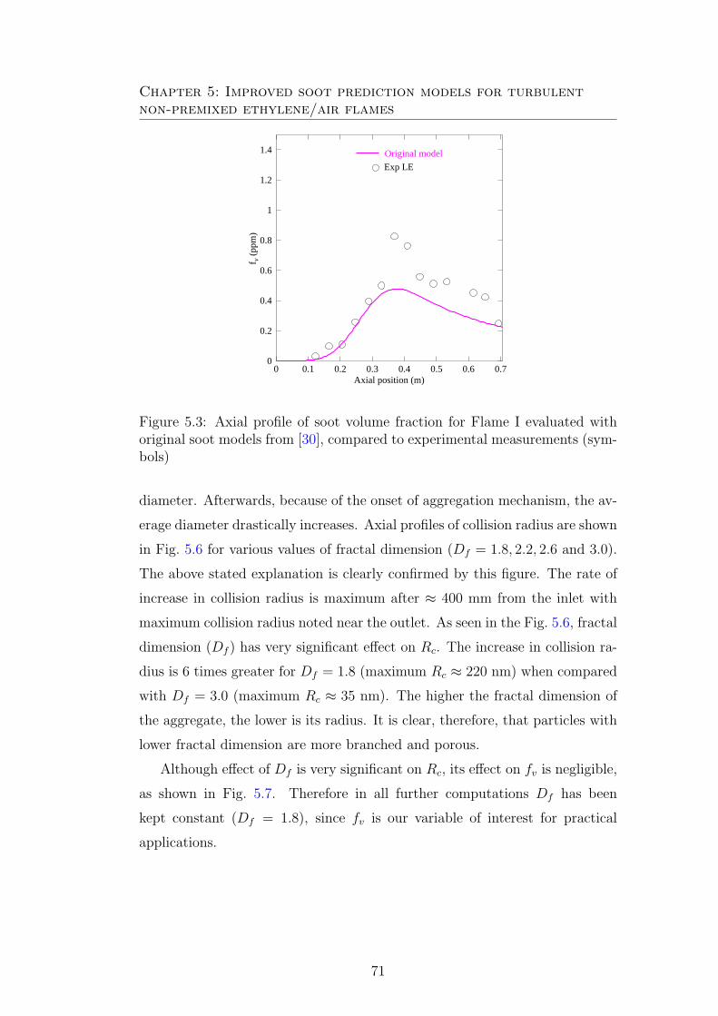
Chapter 5: Improved soot prediction models for turbulentnon-premixed ethylene/air flames
0 0.1 0.2 0.3 0.4 0.5 0.6 0.7Axial position (m)
0
0.2
0.4
0.6
0.8
1
1.2
1.4
f v (
ppm
)
Exp LE
Original model
Figure 5.3: Axial profile of soot volume fraction for Flame I evaluated withoriginal soot models from [30], compared to experimental measurements (sym-bols)
diameter. Afterwards, because of the onset of aggregation mechanism, the av-
erage diameter drastically increases. Axial profiles of collision radius are shown
in Fig. 5.6 for various values of fractal dimension (Df = 1.8, 2.2, 2.6 and 3.0).
The above stated explanation is clearly confirmed by this figure. The rate of
increase in collision radius is maximum after ≈ 400 mm from the inlet with
maximum collision radius noted near the outlet. As seen in the Fig. 5.6, fractal
dimension (Df ) has very significant effect on Rc. The increase in collision ra-
dius is 6 times greater for Df = 1.8 (maximum Rc ≈ 220 nm) when compared
with Df = 3.0 (maximum Rc ≈ 35 nm). The higher the fractal dimension of
the aggregate, the lower is its radius. It is clear, therefore, that particles with
lower fractal dimension are more branched and porous.
Although effect of Df is very significant on Rc, its effect on fv is negligible,
as shown in Fig. 5.7. Therefore in all further computations Df has been
kept constant (Df = 1.8), since fv is our variable of interest for practical
applications.
71

Chapter 5: Improved soot prediction models for turbulentnon-premixed ethylene/air flames
0 0.1 0.2 0.3 0.4 0.5 0.6 0.7Axial position (m)
400
800
1200
1600
2000
2400
T (
K)
Original model
Experimental
Figure 5.4: Axial profile of temperature for Flame I evaluated from originalsoot models
220
9
62
114
167
Figure 5.5: Contour plots of collision radius (Rc, in nm) for fixed fractaldimension, Df = 1.8
72
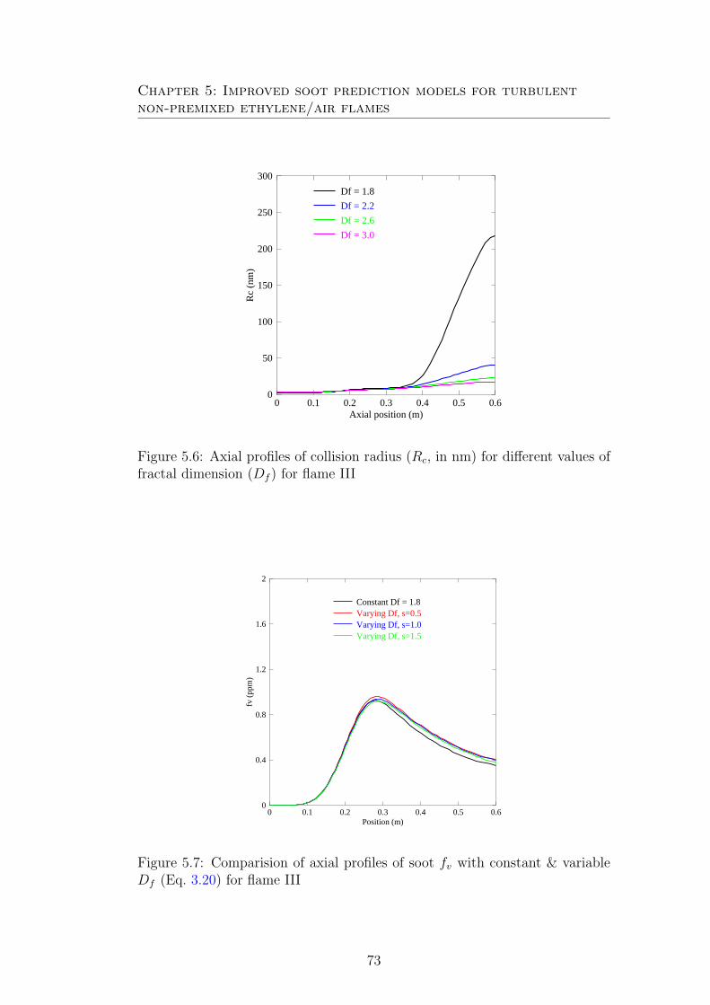
Chapter 5: Improved soot prediction models for turbulentnon-premixed ethylene/air flames
0 0.1 0.2 0.3 0.4 0.5 0.6Axial position (m)
0
50
100
150
200
250
300
Rc
(nm
)
Df = 1.8
Df = 2.2
Df = 2.6
Df = 3.0
Figure 5.6: Axial profiles of collision radius (Rc, in nm) for different values offractal dimension (Df ) for flame III
0 0.1 0.2 0.3 0.4 0.5 0.6Position (m)
0
0.4
0.8
1.2
1.6
2
fv (
ppm
)
Constant Df = 1.8Varying Df, s=0.5Varying Df, s=1.0Varying Df, s=1.5
Figure 5.7: Comparision of axial profiles of soot fv with constant & variableDf (Eq. 3.20) for flame III
73

Chapter 5: Improved soot prediction models for turbulentnon-premixed ethylene/air flames
The soot models are now improved in three successive optimization steps.
The next sections describe the different optimization cases, which differ mainly
in the gas phase combustion model and/or in the optimization parameters.
These cases are referred here as Optimization-Case I to Optimization-Case III.
5.3 Optimization-Case I
The emphasis in this case is completely on the particulate phase and not on
gas-phase kinetics. Therefore, gas-phase chemistry is simply modeled with a
mixture fraction approach combined with equilibrium chemistry, while turbulence-
chemistry interactions are taken into account by a presumed β-PDF. The
evolution of soot particles is described by physical models accounting for nu-
cleation, surface growth, aggregation and oxidation. The Direct Quadrature
Method of Moments is employed to solve the Population Balance Equations in
a computationally efficient manner, assuming a mono-variate PBE with par-
ticle diameter as internal coordinate. The original soot model is optimized
numerically by using Genetic Algorithms coupled with Computational Fluid
Dynamics (CFD). The values of three model parameters, associated with nu-
cleation, oxidation and soot particle radiation are optimized through compar-
ison with recent experimental results. Two objective functions are formulated
based on the difference between experimental and simulation results for tem-
perature and soot volume fraction. After obtaining an optimal parameter set,
the resulting model is further tested against three experimental configurations,
leading to a good agreement and thus demonstrating a high level of generality.
The multi-objective optimization is carried out by considering two objective
functions and three free model parameters. The two objective functions are
the differences between experimental data and simulation results concerning
the fields of temperature and of soot volume fraction (see Section 4.1, on page
61). The three free parameters have been selected after a sensitivity analysis of
each model parameter appearing in the original formulation [30]. Optimization
is based on the experimental results of [50], while three additional flame types
are used to further ascertain the generality of the optimized solution.
74
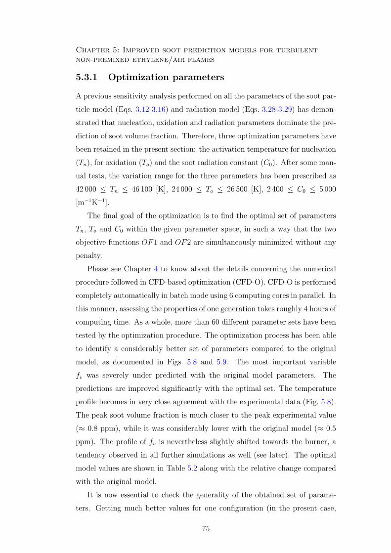
Chapter 5: Improved soot prediction models for turbulentnon-premixed ethylene/air flames
5.3.1 Optimization parameters
A previous sensitivity analysis performed on all the parameters of the soot par-
ticle model (Eqs. 3.12-3.16) and radiation model (Eqs. 3.28-3.29) has demon-
strated that nucleation, oxidation and radiation parameters dominate the pre-
diction of soot volume fraction. Therefore, three optimization parameters have
been retained in the present section: the activation temperature for nucleation
(Tn), for oxidation (To) and the soot radiation constant (C0). After some man-
ual tests, the variation range for the three parameters has been prescribed as
42 000 ≤ Tn ≤ 46 100 [K], 24 000 ≤ To ≤ 26 500 [K], 2 400 ≤ C0 ≤ 5 000
[m−1K−1].
The final goal of the optimization is to find the optimal set of parameters
Tn, To and C0 within the given parameter space, in such a way that the two
objective functions OF1 and OF2 are simultaneously minimized without any
penalty.
Please see Chapter 4 to know about the details concerning the numerical
procedure followed in CFD-based optimization (CFD-O). CFD-O is performed
completely automatically in batch mode using 6 computing cores in parallel. In
this manner, assessing the properties of one generation takes roughly 4 hours of
computing time. As a whole, more than 60 different parameter sets have been
tested by the optimization procedure. The optimization process has been able
to identify a considerably better set of parameters compared to the original
model, as documented in Figs. 5.8 and 5.9. The most important variable
fv was severely under predicted with the original model parameters. The
predictions are improved significantly with the optimal set. The temperature
profile becomes in very close agreement with the experimental data (Fig. 5.8).
The peak soot volume fraction is much closer to the peak experimental value
(≈ 0.8 ppm), while it was considerably lower with the original model (≈ 0.5
ppm). The profile of fv is nevertheless slightly shifted towards the burner, a
tendency observed in all further simulations as well (see later). The optimal
model values are shown in Table 5.2 along with the relative change compared
with the original model.
It is now essential to check the generality of the obtained set of parame-
ters. Getting much better values for one configuration (in the present case,
75
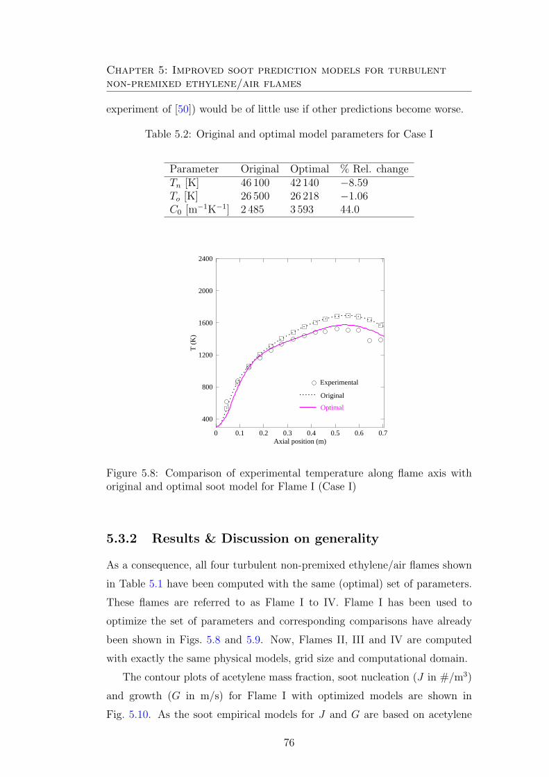
Chapter 5: Improved soot prediction models for turbulentnon-premixed ethylene/air flames
experiment of [50]) would be of little use if other predictions become worse.
Table 5.2: Original and optimal model parameters for Case I
Parameter Original Optimal % Rel. changeTn [K] 46 100 42 140 −8.59To [K] 26 500 26 218 −1.06C0 [m−1K−1] 2 485 3 593 44.0
0 0.1 0.2 0.3 0.4 0.5 0.6 0.7Axial position (m)
400
800
1200
1600
2000
2400
T (
K)
Experimental
Original
Optimal
Figure 5.8: Comparison of experimental temperature along flame axis withoriginal and optimal soot model for Flame I (Case I)
5.3.2 Results & Discussion on generality
As a consequence, all four turbulent non-premixed ethylene/air flames shown
in Table 5.1 have been computed with the same (optimal) set of parameters.
These flames are referred to as Flame I to IV. Flame I has been used to
optimize the set of parameters and corresponding comparisons have already
been shown in Figs. 5.8 and 5.9. Now, Flames II, III and IV are computed
with exactly the same physical models, grid size and computational domain.
The contour plots of acetylene mass fraction, soot nucleation (J in #/m3)
and growth (G in m/s) for Flame I with optimized models are shown in
Fig. 5.10. As the soot empirical models for J and G are based on acetylene
76

Chapter 5: Improved soot prediction models for turbulentnon-premixed ethylene/air flames
0 0.1 0.2 0.3 0.4 0.5 0.6 0.7Axial position (m)
0
0.2
0.4
0.6
0.8
1
1.2
1.4
f v (
ppm
)
Exp LE
Original
Optimal
Figure 5.9: Comparison of experimental soot volume fraction fv along flameaxis with original and optimal soot model for Flame I (Case I)
species, they are active in and around the regions of high acetylene mass frac-
tion. The contours of growth rate are observed to follow closely the acetylene
concentration.
In Fig. 5.11 axial profiles of soot volume fraction are shown for Flame II.
Experimental data are compared with simulation results both with the orig-
inal and with the optimal model parameters. Using the original model, the
predicted peak value of fv is nearly 40% lower than experimental data. The
optimal parameter set predicts almost exactly the peak soot volume fraction,
while a slight shift in peak position towards the burner is again observed.
Axial profiles of temperature and soot volume fraction are shown for Flame III
in Figs. 5.12 and 5.13, respectively. Once again, the agreement concerning
temperature is tremendously better with the optimal model compared to the
original formulation (Fig. 5.12). Simultaneously, the peak soot volume fraction
is also better predicted with the optimal parameter set, while a shift towards
an earlier soot production is again observed (Fig. 5.13). Note that these mea-
surements are more than 20 years old and might therefore be associated with
a higher experimental uncertainty, explaining larger differences between mea-
surements and simulations, independently from the retained numerical model.
Figure 5.14 illustrates the contours of temperature (in K) and soot volume
77
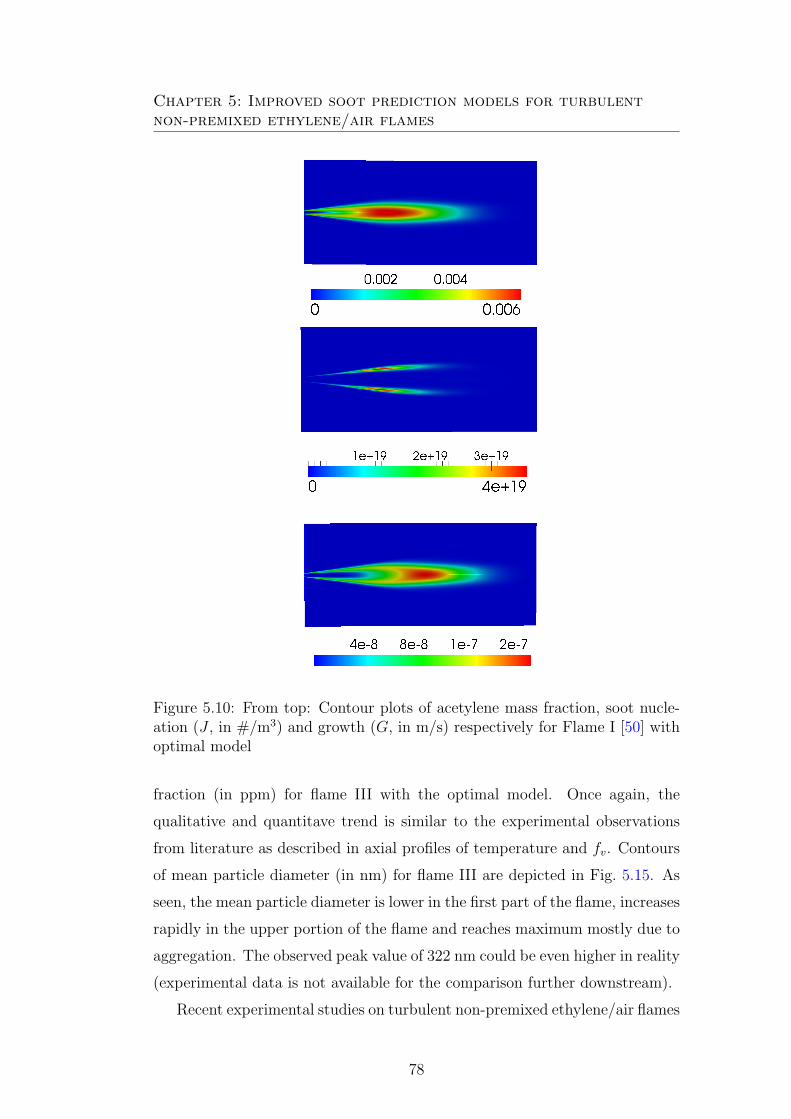
Chapter 5: Improved soot prediction models for turbulentnon-premixed ethylene/air flames
Figure 5.10: From top: Contour plots of acetylene mass fraction, soot nucle-ation (J , in #/m3) and growth (G, in m/s) respectively for Flame I [50] withoptimal model
fraction (in ppm) for flame III with the optimal model. Once again, the
qualitative and quantitave trend is similar to the experimental observations
from literature as described in axial profiles of temperature and fv. Contours
of mean particle diameter (in nm) for flame III are depicted in Fig. 5.15. As
seen, the mean particle diameter is lower in the first part of the flame, increases
rapidly in the upper portion of the flame and reaches maximum mostly due to
aggregation. The observed peak value of 322 nm could be even higher in reality
(experimental data is not available for the comparison further downstream).
Recent experimental studies on turbulent non-premixed ethylene/air flames
78
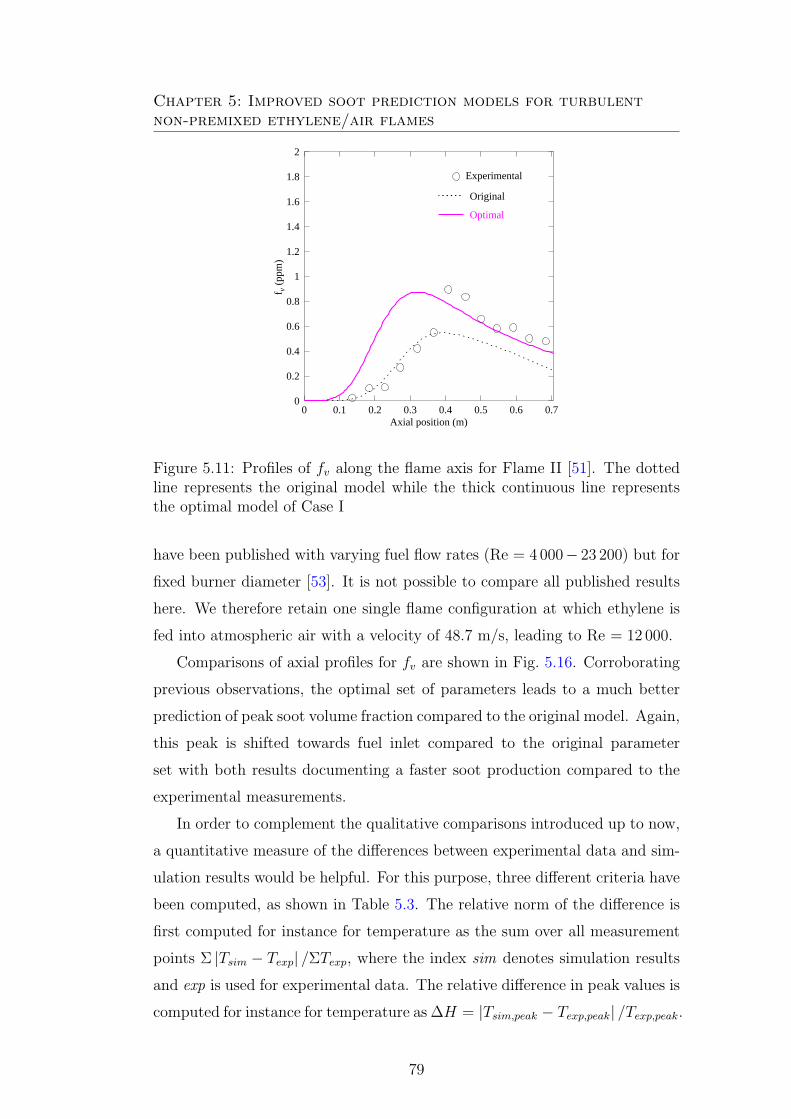
Chapter 5: Improved soot prediction models for turbulentnon-premixed ethylene/air flames
0 0.1 0.2 0.3 0.4 0.5 0.6 0.7Axial position (m)
0
0.2
0.4
0.6
0.8
1
1.2
1.4
1.6
1.8
2
f v (
ppm
)
Experimental
Original
Optimal
Figure 5.11: Profiles of fv along the flame axis for Flame II [51]. The dottedline represents the original model while the thick continuous line representsthe optimal model of Case I
have been published with varying fuel flow rates (Re = 4 000− 23 200) but for
fixed burner diameter [53]. It is not possible to compare all published results
here. We therefore retain one single flame configuration at which ethylene is
fed into atmospheric air with a velocity of 48.7 m/s, leading to Re = 12 000.
Comparisons of axial profiles for fv are shown in Fig. 5.16. Corroborating
previous observations, the optimal set of parameters leads to a much better
prediction of peak soot volume fraction compared to the original model. Again,
this peak is shifted towards fuel inlet compared to the original parameter
set with both results documenting a faster soot production compared to the
experimental measurements.
In order to complement the qualitative comparisons introduced up to now,
a quantitative measure of the differences between experimental data and sim-
ulation results would be helpful. For this purpose, three different criteria have
been computed, as shown in Table 5.3. The relative norm of the difference is
first computed for instance for temperature as the sum over all measurement
points Σ |Tsim − Texp| /ΣTexp, where the index sim denotes simulation results
and exp is used for experimental data. The relative difference in peak values is
computed for instance for temperature as ∆H = |Tsim,peak − Texp,peak| /Texp,peak.
79

Chapter 5: Improved soot prediction models for turbulentnon-premixed ethylene/air flames
0 0.1 0.2 0.3 0.4 0.5 0.6 0.7Axial position (m)
400
800
1200
1600
2000
2400
T (
K)
Experimental
Original
Optimal
Figure 5.12: Profiles of temperature along the flame axis for Flame III [52].The dotted line represents the original model while the thick continuous linerepresents the optimal model of Case I
It can be clearly observed from Table 5.3 that the optimal set of param-
eters leads to a systematic improvement concerning the prediction of peak
temperature but also of peak soot volume fraction, the essential criterion for
practical applications. Furthermore, the full profiles are also in better agree-
ment for Flame I and Flame III concerning temperature as well as soot volume
fraction. Concerning Flames II and IV, the improvement is not as clear, since
temperature fields are not known and due to the observed shift towards the
burner induced by the optimal set of model parameters. The shape of the
profile for fv is indeed better with the optimal set, but getting rid of the shift
should be the next step towards an excellent prediction of soot particles. For
this purpose, additional free parameters must be considered in the optimiza-
tion process.
80
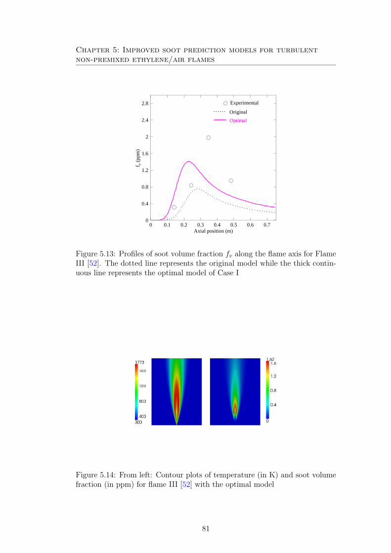
Chapter 5: Improved soot prediction models for turbulentnon-premixed ethylene/air flames
0 0.1 0.2 0.3 0.4 0.5 0.6 0.7Axial position (m)
0
0.4
0.8
1.2
1.6
2
2.4
2.8
f v (
ppm
)
Experimental
Original
Optimal
Figure 5.13: Profiles of soot volume fraction fv along the flame axis for FlameIII [52]. The dotted line represents the original model while the thick contin-uous line represents the optimal model of Case I
Figure 5.14: From left: Contour plots of temperature (in K) and soot volumefraction (in ppm) for flame III [52] with the optimal model
81
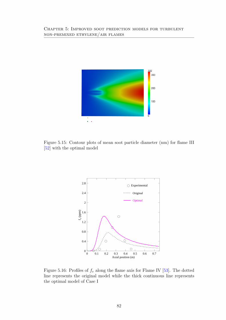
Chapter 5: Improved soot prediction models for turbulentnon-premixed ethylene/air flames
Figure 5.15: Contour plots of mean soot particle diameter (nm) for flame III[52] with the optimal model
0 0.1 0.2 0.3 0.4 0.5 0.6 0.7Axial position (m)
0
0.4
0.8
1.2
1.6
2
2.4
2.8
f v (
ppm
)
Experimental
Original
Optimal
Figure 5.16: Profiles of fv along the flame axis for Flame IV [53]. The dottedline represents the original model while the thick continuous line representsthe optimal model of Case I
82
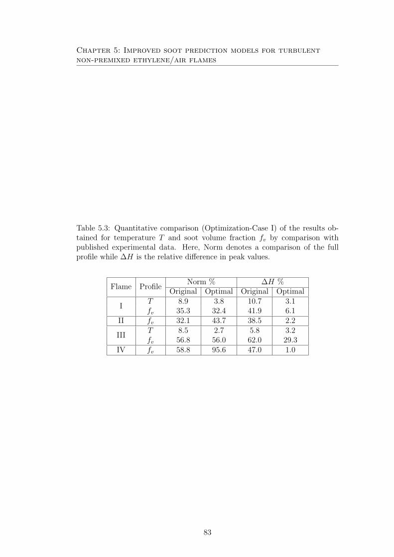
Chapter 5: Improved soot prediction models for turbulentnon-premixed ethylene/air flames
Table 5.3: Quantitative comparison (Optimization-Case I) of the results ob-tained for temperature T and soot volume fraction fv by comparison withpublished experimental data. Here, Norm denotes a comparison of the fullprofile while ∆H is the relative difference in peak values.
Flame ProfileNorm % ∆H %
Original Optimal Original Optimal
IT 8.9 3.8 10.7 3.1fv 35.3 32.4 41.9 6.1
II fv 32.1 43.7 38.5 2.2
IIIT 8.5 2.7 5.8 3.2fv 56.8 56.0 62.0 29.3
IV fv 58.8 95.6 47.0 1.0
83

Chapter 5: Improved soot prediction models for turbulentnon-premixed ethylene/air flames
5.4 Optimization-Case II
5.5 Parameters and objective functions
In the second optimization step, there were several changes and improvements
compared to the earlier optimization (Optimization-Case I) in an effort to
remove the undesirable profile shift towards the burner. This study is in-turn
divided in to two different cases as described below (Case II-1 and Case II-2).
Case II-1: 3 objective functions (OF1,OF2,OF3), 3 model pa-
rameters
• OF2 is evaluated with respect to LE measurement only instead of aver-
age between LE and TEM (see again Fig. 5.9, on page 77).
• An additional objective function (OF3) has been included from the fv
exmperimental data of flame IV similarly to OF2.
• Combustion is represented again with equilibrium chemistry
Case II-2: 2 objective functions (OF1,OF2), 4 model parameters
• OF2 is again evaluated with respect to LE measurement points only.
• Combustion is now modeled with a more accurate laminar flamelet mod-
eling
• An additional optimization parameter (Tg) has been added.
The objective functions are evaluated exactly in the same manner as earlier
(see Chapter 4), i.e., based on the difference between the obtained simulation
results and experimental measurements of temperature and soot volume frac-
tion (from LE). After obtaining an optimal parameter set, the resulting models
are further tested against the three independent experimental configurations
in order to check generality.
5.5.1 Results & discussion
Some numerical details of the two optimization runs are first discussed. For
Case II-1, CFD-based optimization has been carried out during 11 genera-
84
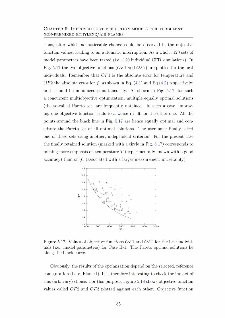
Chapter 5: Improved soot prediction models for turbulentnon-premixed ethylene/air flames
tions, after which no noticeable change could be observed in the objective
function values, leading to an automatic interruption. As a whole, 120 sets of
model parameters have been tested (i.e., 120 individual CFD simulations). In
Fig. 5.17 the two objective functions (OF1 and OF2) are plotted for the best
individuals. Remember that OF1 is the absolute error for temperature and
OF2 the absolute error for fv as shown in Eq. (4.1) and Eq.(4.2) respectively;
both should be minimized simultaneously. As shown in Fig. 5.17, for such
a concurrent multiobjective optimization, multiple equally optimal solutions
(the so-called Pareto set) are frequently obtained. In such a case, improv-
ing one objective function leads to a worse result for the other one. All the
points around the black line in Fig. 5.17 are hence equally optimal and con-
stitute the Pareto set of all optimal solutions. The user must finally select
one of these sets using another, independent criterion. For the present case
the finally retained solution (marked with a circle in Fig. 5.17) corresponds to
putting more emphasis on temperature T (experimentally known with a good
accuracy) than on fv (associated with a larger measurement uncertainty).
400 500 600 700 800 900 1000 OF1
1.2
1.4
1.6
1.8
2
2.2
2.4
2.6
2.8
OF2
Figure 5.17: Values of objective functions OF1 and OF2 for the best individ-uals (i.e., model parameters) for Case II-1. The Pareto optimal solutions liealong the black curve.
Obviously, the results of the optimization depend on the selected, reference
configuration (here, Flame I). It is therefore interesting to check the impact of
this (arbitrary) choice. For this purpose, Figure 5.18 shows objective function
values called OF2 and OF3 plotted against each other. Objective function
85
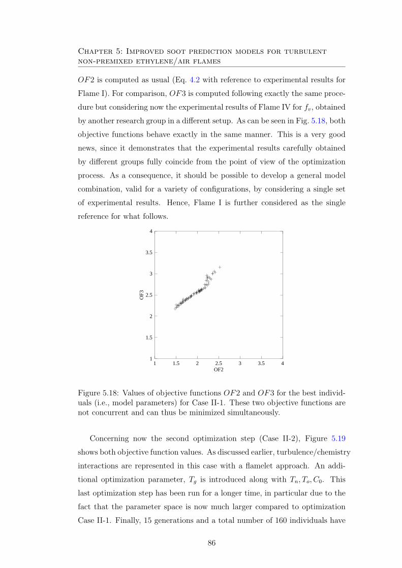
Chapter 5: Improved soot prediction models for turbulentnon-premixed ethylene/air flames
OF2 is computed as usual (Eq. 4.2 with reference to experimental results for
Flame I). For comparison, OF3 is computed following exactly the same proce-
dure but considering now the experimental results of Flame IV for fv, obtained
by another research group in a different setup. As can be seen in Fig. 5.18, both
objective functions behave exactly in the same manner. This is a very good
news, since it demonstrates that the experimental results carefully obtained
by different groups fully coincide from the point of view of the optimization
process. As a consequence, it should be possible to develop a general model
combination, valid for a variety of configurations, by considering a single set
of experimental results. Hence, Flame I is further considered as the single
reference for what follows.
1 1.5 2 2.5 3 3.5 4 OF2
1
1.5
2
2.5
3
3.5
4
OF
3
Figure 5.18: Values of objective functions OF2 and OF3 for the best individ-uals (i.e., model parameters) for Case II-1. These two objective functions arenot concurrent and can thus be minimized simultaneously.
Concerning now the second optimization step (Case II-2), Figure 5.19
shows both objective function values. As discussed earlier, turbulence/chemistry
interactions are represented in this case with a flamelet approach. An addi-
tional optimization parameter, Tg is introduced along with Tn, To, C0. This
last optimization step has been run for a longer time, in particular due to the
fact that the parameter space is now much larger compared to optimization
Case II-1. Finally, 15 generations and a total number of 160 individuals have
86
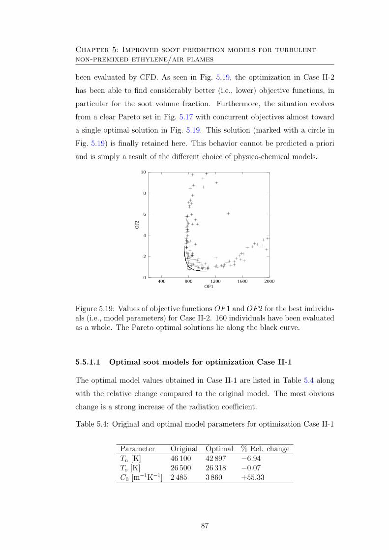
Chapter 5: Improved soot prediction models for turbulentnon-premixed ethylene/air flames
been evaluated by CFD. As seen in Fig. 5.19, the optimization in Case II-2
has been able to find considerably better (i.e., lower) objective functions, in
particular for the soot volume fraction. Furthermore, the situation evolves
from a clear Pareto set in Fig. 5.17 with concurrent objectives almost toward
a single optimal solution in Fig. 5.19. This solution (marked with a circle in
Fig. 5.19) is finally retained here. This behavior cannot be predicted a priori
and is simply a result of the different choice of physico-chemical models.
400 800 1200 1600 2000OF1
0
2
4
6
8
10
OF2
Figure 5.19: Values of objective functions OF1 and OF2 for the best individu-als (i.e., model parameters) for Case II-2. 160 individuals have been evaluatedas a whole. The Pareto optimal solutions lie along the black curve.
5.5.1.1 Optimal soot models for optimization Case II-1
The optimal model values obtained in Case II-1 are listed in Table 5.4 along
with the relative change compared to the original model. The most obvious
change is a strong increase of the radiation coefficient.
Table 5.4: Original and optimal model parameters for optimization Case II-1
Parameter Original Optimal % Rel. changeTn [K] 46 100 42 897 −6.94To [K] 26 500 26 318 −0.07C0 [m−1K−1] 2 485 3 860 +55.33
87

Chapter 5: Improved soot prediction models for turbulentnon-premixed ethylene/air flames
0 0.1 0.2 0.3 0.4 0.5 0.6 0.7Axial position (m)
400
800
1200
1600
2000
T (
K)
Experimental
Original
Optimal, Case II-1
Optimal, Case II-2
eiei+1
Figure 5.20: Comparison of experimental temperature along flame axis withoriginal and optimal soot models (Case II) for Flame I. Measurements by [50].
Comparisons are shown in Figs. 5.20 and 5.21 concerning Flame I which is
always used to optimize the models. With the original models, temperature of
Flame I, was considerably overpredicted while at the same time fv was severely
underpredicted. The results are considerably improved for both quantities
with the optimized model parameters. However, since Flame I was used for
the optimization, the obtained progress is of course not a surprise. It is now
necessary to check that the predictions improve also for other, independent
cases. For this purpose, the flames of
Please note that the inclusion of a 3rd objective function (OF3) has not
improved the models any further, since OF2 and OF3 describe the same
physical quantity (fv) and are corelated (see Fig. 5.18). Therefore, in Case II-
2 only 2 objective functions were considered.
In Fig. 5.22 axial profiles of soot volume fraction are shown for Flame II.
Experimental data (symbols) are compared with simulation results both with
the original and with the optimal model parameters of Case II-1. Using the
original models, the predicted peak value of fv is nearly 40% lower than the
experimental data. The predictions with the optimal models improve consider-
ably the peak soot volume fraction, but a slight shift in peak position towards
the burner is again observed, similar to that already visible in Fig. 5.9.
88

Chapter 5: Improved soot prediction models for turbulentnon-premixed ethylene/air flames
0 0.1 0.2 0.3 0.4 0.5 0.6 0.7Axial position (m)
0
0.2
0.4
0.6
0.8
1
1.2
f v (
ppm
)
Exp LE
Original
Optimal, Case II-1
Optimal, Case II-2
Ei Ei+1
Figure 5.21: Comparison of experimental soot volume fraction fv along flameaxis with original and optimal soot models (Case II) for Flame I. Measurementsby [50].
Axial profiles of soot volume fraction are shown for Flame III in Fig. 5.23.
It is clear that the peak soot volume fraction is considerably better predicted
with the optimal parameter sets. However, a slight shift for the profile of fv
towards the burner is again found. At the same time, the agreement concerning
temperature is tremendously better with the optimal models compared to the
original formulation (figure not shown).
For Flame IV one single flame configuration at which ethylene is fed into
atmospheric air with a velocity of 48.7 m/s has been retained (see Table 5.1,
on page 69), leading to Re = 12 000. Comparisons of axial profiles for fv are
shown in Fig. 5.24. Corroborating previous observations, the optimal set of
parameters leads to a much better prediction of peak soot volume fraction
compared to the original models. But again, this peak is slightly shifted to-
wards fuel inlet compared to the original parameter set. Both original and
optimal model parameters lead to a faster soot production compared to the
experimental measurements.
In order to complement the purely qualitative comparisons introduced up
to now, a quantitative measure of the differences between experimental data
and simulation results is helpful. For this purpose, the same criteria have been
89
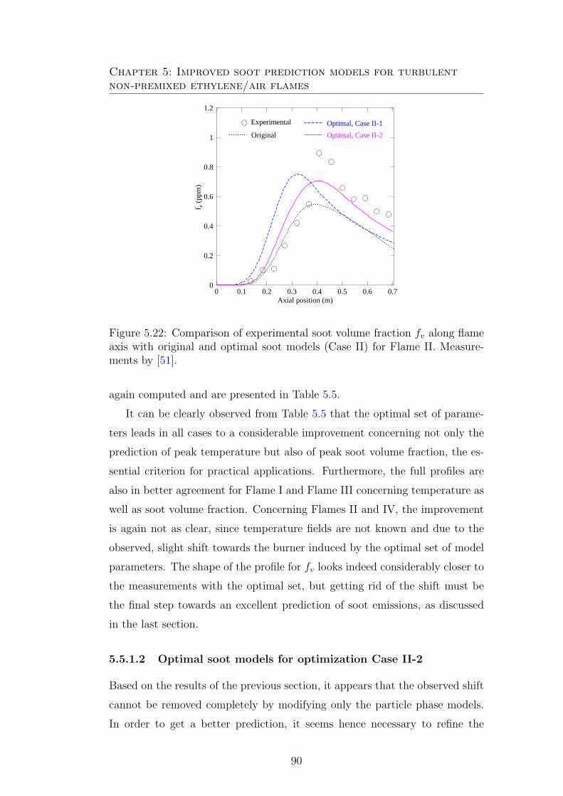
Chapter 5: Improved soot prediction models for turbulentnon-premixed ethylene/air flames
0 0.1 0.2 0.3 0.4 0.5 0.6 0.7Axial position (m)
0
0.2
0.4
0.6
0.8
1
1.2
f v (
ppm
)
Experimental
Original
Optimal, Case II-1
Optimal, Case II-2
Figure 5.22: Comparison of experimental soot volume fraction fv along flameaxis with original and optimal soot models (Case II) for Flame II. Measure-ments by [51].
again computed and are presented in Table 5.5.
It can be clearly observed from Table 5.5 that the optimal set of parame-
ters leads in all cases to a considerable improvement concerning not only the
prediction of peak temperature but also of peak soot volume fraction, the es-
sential criterion for practical applications. Furthermore, the full profiles are
also in better agreement for Flame I and Flame III concerning temperature as
well as soot volume fraction. Concerning Flames II and IV, the improvement
is again not as clear, since temperature fields are not known and due to the
observed, slight shift towards the burner induced by the optimal set of model
parameters. The shape of the profile for fv looks indeed considerably closer to
the measurements with the optimal set, but getting rid of the shift must be
the final step towards an excellent prediction of soot emissions, as discussed
in the last section.
5.5.1.2 Optimal soot models for optimization Case II-2
Based on the results of the previous section, it appears that the observed shift
cannot be removed completely by modifying only the particle phase models.
In order to get a better prediction, it seems hence necessary to refine the
90

Chapter 5: Improved soot prediction models for turbulentnon-premixed ethylene/air flames
0 0.1 0.2 0.3 0.4 0.5 0.6 0.7Axial position (m)
0
0.4
0.8
1.2
1.6
2
2.4
f v (
ppm
)
Experimental
Original
Optimal, Case II-1
Optimal, Case II-2
Figure 5.23: Comparison of experimental soot volume fraction fv along flameaxis with original and optimal soot models (Case II) for Flame III. Measure-ments by [52].
description of the physico-chemical processes in the gas phase. This is why
turbulence/chemistry coupling is now realized with a flamelet model. A suit-
able set of model parameters can then hopefully be identified by adding the
activation temperature for growth as an optimization parameter and by pre-
scribing a very large parameter space. The model parameter values finally
obtained by the optimization in Case II-2 are listed in Table 5.6 (see, page
93). Compared to the results of Table 5.4 (see, page 87), it is clear that much
larger deviations have been tolerated in this final optimization step, compared
to the original models of the literature. Radiation and particle growth are
very strongly impacted. But, since the corresponding parameters appear in
an exponential function, nucleation and even oxidation are also strongly mod-
ified. Since all models are coupled and all parameters are relevant for the
objective functions, it seems logical that the optimizer will have to play on all
parameters simultaneously in order to improve the predictions.
Considering first Flame I, the corresponding comparisons with the exper-
imental data for temperature and fv have been already shown in Figs. 5.20
and 5.21 respectively. The agreement is nearly perfect for soot volume frac-
tion and as good as before for temperature, being in particular closer to the
91
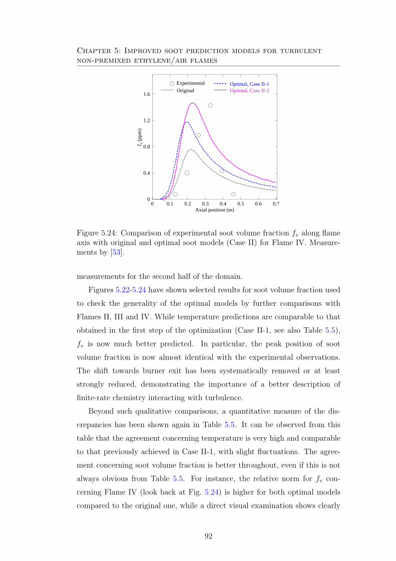
Chapter 5: Improved soot prediction models for turbulentnon-premixed ethylene/air flames
0 0.1 0.2 0.3 0.4 0.5 0.6 0.7Axial position (m)
0
0.4
0.8
1.2
1.6
f v (
ppm
)
Experimental
OriginalOptimal, Case II-1Optimal, Case II-2
Figure 5.24: Comparison of experimental soot volume fraction fv along flameaxis with original and optimal soot models (Case II) for Flame IV. Measure-ments by [53].
measurements for the second half of the domain.
Figures 5.22-5.24 have shown selected results for soot volume fraction used
to check the generality of the optimal models by further comparisons with
Flames II, III and IV. While temperature predictions are comparable to that
obtained in the first step of the optimization (Case II-1, see also Table 5.5),
fv is now much better predicted. In particular, the peak position of soot
volume fraction is now almost identical with the experimental observations.
The shift towards burner exit has been systematically removed or at least
strongly reduced, demonstrating the importance of a better description of
finite-rate chemistry interacting with turbulence.
Beyond such qualitative comparisons, a quantitative measure of the dis-
crepancies has been shown again in Table 5.5. It can be observed from this
table that the agreement concerning temperature is very high and comparable
to that previously achieved in Case II-1, with slight fluctuations. The agree-
ment concerning soot volume fraction is better throughout, even if this is not
always obvious from Table 5.5. For instance, the relative norm for fv con-
cerning Flame IV (look back at Fig. 5.24) is higher for both optimal models
compared to the original one, while a direct visual examination shows clearly
92
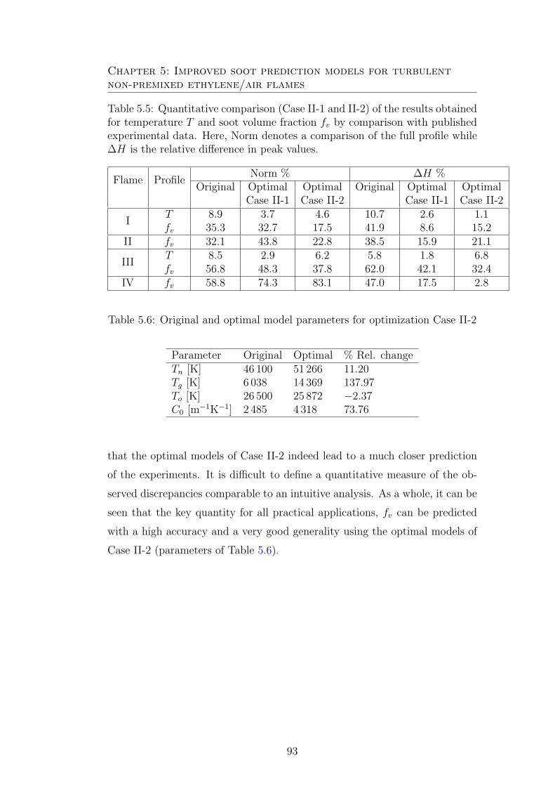
Chapter 5: Improved soot prediction models for turbulentnon-premixed ethylene/air flames
Table 5.5: Quantitative comparison (Case II-1 and II-2) of the results obtainedfor temperature T and soot volume fraction fv by comparison with publishedexperimental data. Here, Norm denotes a comparison of the full profile while∆H is the relative difference in peak values.
Flame ProfileNorm % ∆H %
Original Optimal Optimal Original Optimal OptimalCase II-1 Case II-2 Case II-1 Case II-2
IT 8.9 3.7 4.6 10.7 2.6 1.1fv 35.3 32.7 17.5 41.9 8.6 15.2
II fv 32.1 43.8 22.8 38.5 15.9 21.1
IIIT 8.5 2.9 6.2 5.8 1.8 6.8fv 56.8 48.3 37.8 62.0 42.1 32.4
IV fv 58.8 74.3 83.1 47.0 17.5 2.8
Table 5.6: Original and optimal model parameters for optimization Case II-2
Parameter Original Optimal % Rel. changeTn [K] 46 100 51 266 11.20Tg [K] 6 038 14 369 137.97To [K] 26 500 25 872 −2.37C0 [m−1K−1] 2 485 4 318 73.76
that the optimal models of Case II-2 indeed lead to a much closer prediction
of the experiments. It is difficult to define a quantitative measure of the ob-
served discrepancies comparable to an intuitive analysis. As a whole, it can be
seen that the key quantity for all practical applications, fv can be predicted
with a high accuracy and a very good generality using the optimal models of
Case II-2 (parameters of Table 5.6).
93
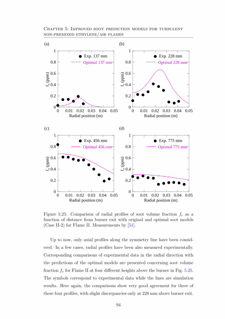
Chapter 5: Improved soot prediction models for turbulentnon-premixed ethylene/air flames
0 0.01 0.02 0.03 0.04 0.05Radial position (m)
0
0.2
0.4
0.6
0.8
1f v
(pp
m)
(a)
Exp. 137 mm
Optimal 137 mm
0 0.01 0.02 0.03 0.04 0.05Radial position (m)
0
0.2
0.4
0.6
0.8
1
f v (
ppm
)
(b)
Exp. 228 mm
Optimal 228 mm
0 0.01 0.02 0.03 0.04 0.05Radial position (m)
0
0.2
0.4
0.6
0.8
1
f v (
ppm
)
(c)
Exp. 456 mm
Optimal 456 mm
0 0.01 0.02 0.03 0.04 0.05Radial position (m)
0
0.2
0.4
0.6
0.8
1
f v (
ppm
)
(d)
Exp. 775 mm
Optimal 775 mm
Figure 5.25: Comparison of radial profiles of soot volume fraction fv as afunction of distance from burner exit with original and optimal soot models(Case II-2) for Flame II. Measurements by [51].
Up to now, only axial profiles along the symmetry line have been consid-
ered. In a few cases, radial profiles have been also measured experimentally.
Corresponding comparisons of experimental data in the radial direction with
the predictions of the optimal models are presented concerning soot volume
fraction fv for Flame II at four different heights above the burner in Fig. 5.25.
The symbols correspond to experimental data while the lines are simulation
results. Here again, the comparisons show very good agreement for three of
these four profiles, with slight discrepancies only at 228 mm above burner exit.
94
Chapter 5: Improved soot prediction models for turbulentnon-premixed ethylene/air flames
The developed model combination appears therefore to be valid for many dif-
ferent configurations.
An even better agreement with experimental measurements might however
be perhaps possible by changing the radiation model, since radiative heat
transfer has a major impact on flame and soot properties.
5.6 Optimization-Case III
5.6.1 Models for radiative heat transfer
Radiative heat transfer is highly significant in combustion processes involving
soot. Due to the tight coupling of employed semi-empirical soot models with
temperature, it is essential to take into account radiative heat transfer asso-
ciated with soot particles as well as with key gaseous species while keeping
acceptable numerical complexity. In the present section, three simple soot
radiation models are analyzed, compared and optimized in an effort to repro-
duce as well as possible published experimental results while keeping intact
the particulate models previously developed.
Please refer to Chapter 3 for a detailed description of the soot radiation
models. C0, C1 and C2 are the three proportionality constants associated with
each radiation model, respectively. Therefore, the only optimization parame-
ter is C0, C1 or C2, respectively. Three independent optimizations have been
carried out, one for each model. In each case the two concurrent objective
functions are the absolute errors of temperature and of fv obtained from sim-
ulation and compared to the experimental data of Flame I, as explained in
Chapter 4.
For a start, Figs. 5.26 and 5.27 illustrate the impact of gas and soot ra-
diative heat transfer on temperature and fv in Flame I, respectively. Without
any radiation, the final temperature is about 800 K too high (Fig. 5.26). Tak-
ing into account soot radiation, a much better agreement is found with the
experimental measurements (shown as circles). When taking additionally into
account gas-phase radiation (solid line), a further decrease of temperature by
≈ 50 − 80 K is observed at the end of the computational domain and the
95
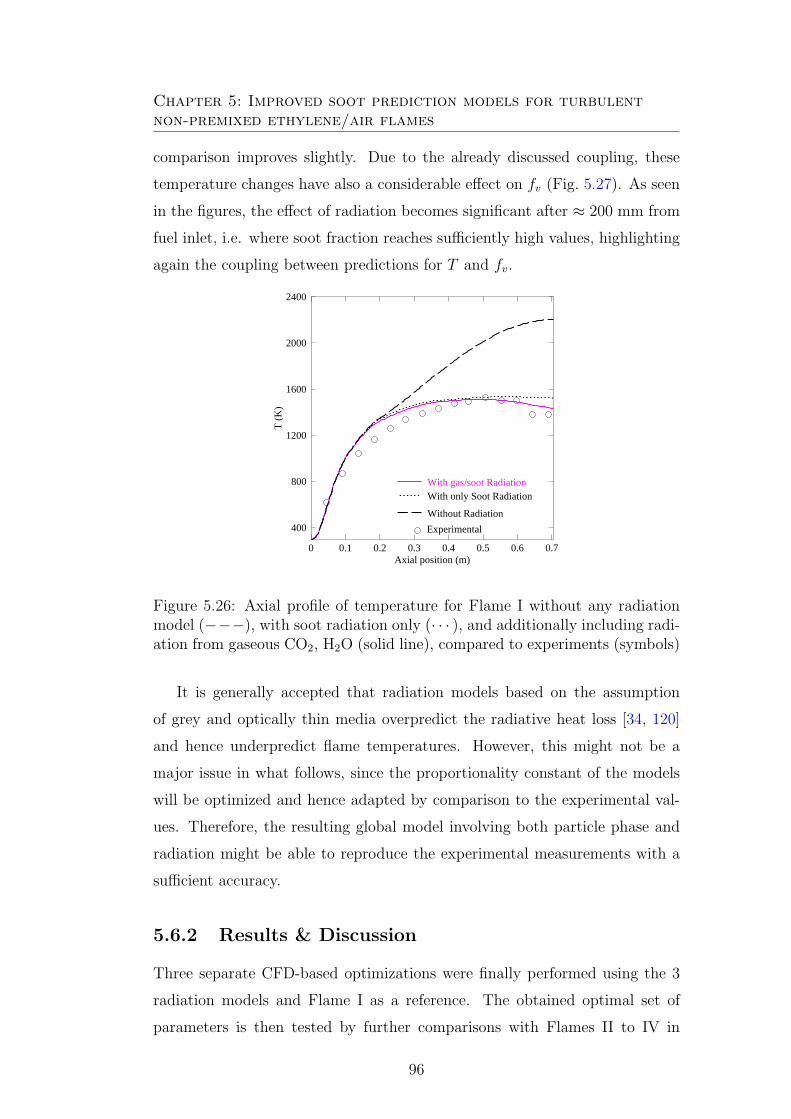
Chapter 5: Improved soot prediction models for turbulentnon-premixed ethylene/air flames
comparison improves slightly. Due to the already discussed coupling, these
temperature changes have also a considerable effect on fv (Fig. 5.27). As seen
in the figures, the effect of radiation becomes significant after ≈ 200 mm from
fuel inlet, i.e. where soot fraction reaches sufficiently high values, highlighting
again the coupling between predictions for T and fv.
0 0.1 0.2 0.3 0.4 0.5 0.6 0.7Axial position (m)
400
800
1200
1600
2000
2400
T (
K)
With gas/soot RadiationWith only Soot Radiation
Without Radiation
Experimental
Figure 5.26: Axial profile of temperature for Flame I without any radiationmodel (−−−), with soot radiation only (· · · ), and additionally including radi-ation from gaseous CO2, H2O (solid line), compared to experiments (symbols)
It is generally accepted that radiation models based on the assumption
of grey and optically thin media overpredict the radiative heat loss [34, 120]
and hence underpredict flame temperatures. However, this might not be a
major issue in what follows, since the proportionality constant of the models
will be optimized and hence adapted by comparison to the experimental val-
ues. Therefore, the resulting global model involving both particle phase and
radiation might be able to reproduce the experimental measurements with a
sufficient accuracy.
5.6.2 Results & Discussion
Three separate CFD-based optimizations were finally performed using the 3
radiation models and Flame I as a reference. The obtained optimal set of
parameters is then tested by further comparisons with Flames II to IV in
96

Chapter 5: Improved soot prediction models for turbulentnon-premixed ethylene/air flames
0 0.1 0.2 0.3 0.4 0.5 0.6 0.7Axial position (m)
0
0.2
0.4
0.6
0.8
1
1.2
1.4
f v (
ppm
)
Exp LE
Without gas Radition
With gas/Soot Radiation
Figure 5.27: Axial profile of fv for Flame I without and with gas radiationfrom CO2 and H2O , compared to experiments (symbols)
order to check the generality of the results.
5.6.2.1 Radiation model I (Eq. 3.29)
Since Radiation model I and the associated parameter C0 have been already
included in earlier optimization studies, we did not expect a large progress,
even when concentrating now all computational resources on C0. Indeed, the
optimization is only able to improve very slightly the temperature profile,
as shown in Fig. 5.28, keeping at the same time a similar agreement for fv,
as shown in Fig. 5.29, improved globally but slightly worse concerning peak
value. When checking generality using Flames II to IV (not shown), the same
conclusion applies; modifications are very slight and do not lead to a clear im-
provement compared to the experimental measurements. It is indeed possible
to get a better agreement for temperature, OF1, by increasing the radiation
parameter C0. However, the associated impact on fv (OF2) is then mostly
negative. As seen in the Pareto optimal set, since the radiational proportion-
ality constant, C0 was already included in the earlier optimization, further
optimization cannot deliver a significant improvement. The increase in pa-
rameter value decreases OF1 (Fig. 5.30) but the trend for OF2 is not uniform
(Figure 5.31).
97

Chapter 5: Improved soot prediction models for turbulentnon-premixed ethylene/air flames
0 0.1 0.2 0.3 0.4 0.5 0.6 0.7Axial position (m)
400
800
1200
1600
2000
2400
T (
K)
Experimental
Optimal
Original
ei
ei+1
Figure 5.28: Comparison of temperature along flame axis with original modeland after optimizing Radiation model I for Flame I
5.6.2.2 Radiation model II (Eq. 3.30)
The optimization results for Radiation model II are documented in Figs. 5.32
and 5.33. Here, it is possible to improve simultaneously the agreement for
temperature and fv, but the progress is very slight. This means that the
originally published value for the radiation factor is directly suitable for the
present application. The same behavior is observed for all other flames as well
(not shown).
5.6.2.3 Radiation model III (Eq. 3.31)
At the difference of the two previous cases, the optimization relying on Ra-
diation model III leads to considerable modifications. The original model pa-
rameter leads to a strong overprediction of fv as exemplified in Fig. 5.34. The
optimization leads to a best possible value of C2 = 5292 m2kg−1. Figure 5.35
shows the resulting temperature for Flame I. Similar changes are observed for
all other flames as well (not shown).
98
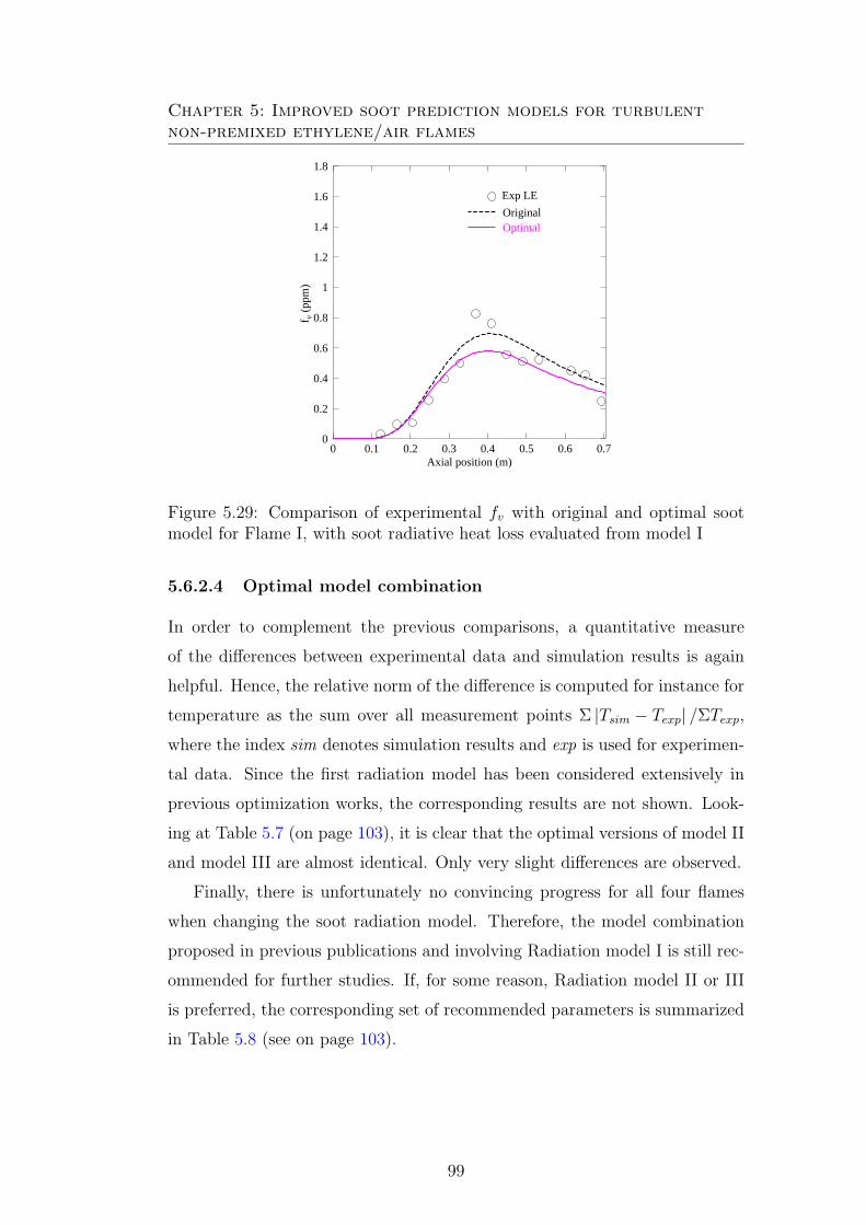
Chapter 5: Improved soot prediction models for turbulentnon-premixed ethylene/air flames
0 0.1 0.2 0.3 0.4 0.5 0.6 0.7Axial position (m)
0
0.2
0.4
0.6
0.8
1
1.2
1.4
1.6
1.8
f v (
ppm
)
Exp LE
OriginalOptimal
Figure 5.29: Comparison of experimental fv with original and optimal sootmodel for Flame I, with soot radiative heat loss evaluated from model I
5.6.2.4 Optimal model combination
In order to complement the previous comparisons, a quantitative measure
of the differences between experimental data and simulation results is again
helpful. Hence, the relative norm of the difference is computed for instance for
temperature as the sum over all measurement points Σ |Tsim − Texp| /ΣTexp,
where the index sim denotes simulation results and exp is used for experimen-
tal data. Since the first radiation model has been considered extensively in
previous optimization works, the corresponding results are not shown. Look-
ing at Table 5.7 (on page 103), it is clear that the optimal versions of model II
and model III are almost identical. Only very slight differences are observed.
Finally, there is unfortunately no convincing progress for all four flames
when changing the soot radiation model. Therefore, the model combination
proposed in previous publications and involving Radiation model I is still rec-
ommended for further studies. If, for some reason, Radiation model II or III
is preferred, the corresponding set of recommended parameters is summarized
in Table 5.8 (see on page 103).
99
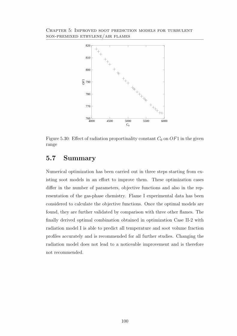
Chapter 5: Improved soot prediction models for turbulentnon-premixed ethylene/air flames
4000 4500 5000 5500 6000C0
760
770
780
790
800
810
820
OF
1
Figure 5.30: Effect of radiation proportinality constant C0 on OF1 in the givenrange
5.7 Summary
Numerical optimization has been carried out in three steps starting from ex-
isting soot models in an effort to improve them. These optimization cases
differ in the number of parameters, objective functions and also in the rep-
resentation of the gas-phase chemistry. Flame I experimental data has been
considered to calculate the objective functions. Once the optimal models are
found, they are further validated by comparison with three other flames. The
finally derived optimal combination obtained in optimization Case II-2 with
radiation model I is able to predict all temperature and soot volume fraction
profiles accurately and is recommended for all further studies. Changing the
radiation model does not lead to a noticeable improvement and is therefore
not recommended.
100

Chapter 5: Improved soot prediction models for turbulentnon-premixed ethylene/air flames
760 770 780 790 800 810 820OF1
0.8
0.9
1
1.1
1.2
OF
2
Figure 5.31: Values of objective functions OF1 and OF2 for the best individ-uals (i.e., model parameters)
0 0.1 0.2 0.3 0.4 0.5 0.6 0.7Axial position (m)
400
800
1200
1600
2000
2400
T (
K)
Experimental
Original
Optimal
Figure 5.32: Comparison of experimental temperature with original and op-timal soot model for Flame I, with soot radiative heat loss evaluated frommodel II
101

Chapter 5: Improved soot prediction models for turbulentnon-premixed ethylene/air flames
0 0.1 0.2 0.3 0.4 0.5 0.6 0.7Axial position (m)
0
0.2
0.4
0.6
0.8
1
1.2
1.4
1.6
1.8
f v (
ppm
)
Experimental
OriginalOptimal
Figure 5.33: Comparison of experimental fv with original and optimal sootmodel for Flame I, with soot radiative heat loss evaluated from model II
0 0.1 0.2 0.3 0.4 0.5 0.6 0.7Axial position (m)
0
0.2
0.4
0.6
0.8
1
1.2
1.4
1.6
1.8
f v (
ppm
)
Experimental
OriginalOptimal
Figure 5.34: Comparison of experimental fv with original and optimal sootmodel for Flame I, with soot radiative heat loss evaluated from model III
102
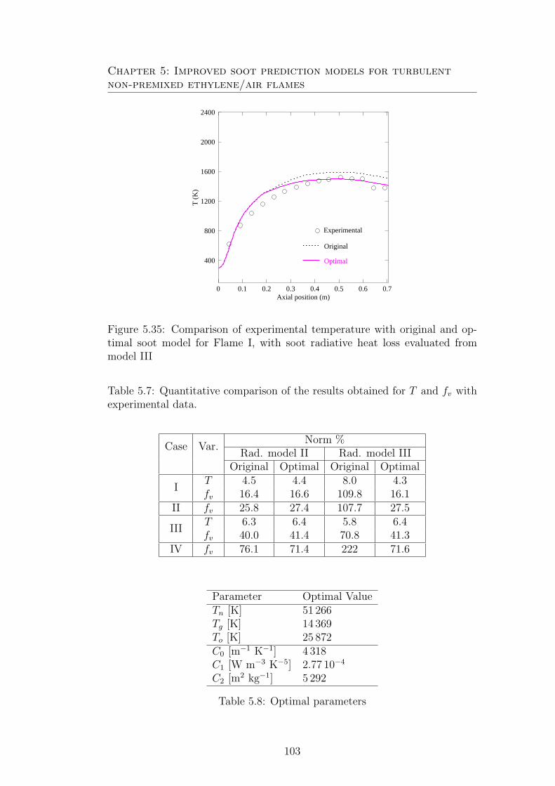
Chapter 5: Improved soot prediction models for turbulentnon-premixed ethylene/air flames
0 0.1 0.2 0.3 0.4 0.5 0.6 0.7Axial position (m)
400
800
1200
1600
2000
2400
T (
K)
Experimental
Original
Optimal
Figure 5.35: Comparison of experimental temperature with original and op-timal soot model for Flame I, with soot radiative heat loss evaluated frommodel III
Table 5.7: Quantitative comparison of the results obtained for T and fv withexperimental data.
Case Var.Norm %
Rad. model II Rad. model IIIOriginal Optimal Original Optimal
IT 4.5 4.4 8.0 4.3fv 16.4 16.6 109.8 16.1
II fv 25.8 27.4 107.7 27.5
IIIT 6.3 6.4 5.8 6.4fv 40.0 41.4 70.8 41.3
IV fv 76.1 71.4 222 71.6
Parameter Optimal ValueTn [K] 51 266Tg [K] 14 369To [K] 25 872C0 [m−1 K−1] 4 318C1 [W m−3 K−5] 2.77 10−4
C2 [m2 kg−1] 5 292
Table 5.8: Optimal parameters
103
Chapter 6
Modeling TiO2 nanoparticle
formation in CH4-O2 diffusion
flames
6.1 Introduction
The present chapter aims at modeling as accurately as possible TiO2 nanopar-
ticle formation in turbulent flames. Due to the vast applications of TiO2
particles (pigments, cosmetics, photocatalysis) understanding its formation
and evolution is very important. Two different precursors are typically used
in the production of TiO2 nanoparticles, titanium tetra-isopropoxide (TTIP)
and titanium tetra-chloride (TiCl4). We decided to concentrate here on TTIP.
Detailed analysis of literature shows that the chemistry behind formation of
nanoparticle nuclei from precursor solution and subsequent growth process are
not satisfactorily well-known or understood yet. Physico-chemical models de-
scribing the formation of TiO2 nanoparticles are very limited in the literature.
Therefore, developing prediction models is very challenging, but relevant for
many applications.
6.2 Configuration
The typical configuration employed for all simulations involves a CH4-O2 dif-
fusion flame with TTIP as precursor and Ar as carrier gas. Figure 6.1 shows
104
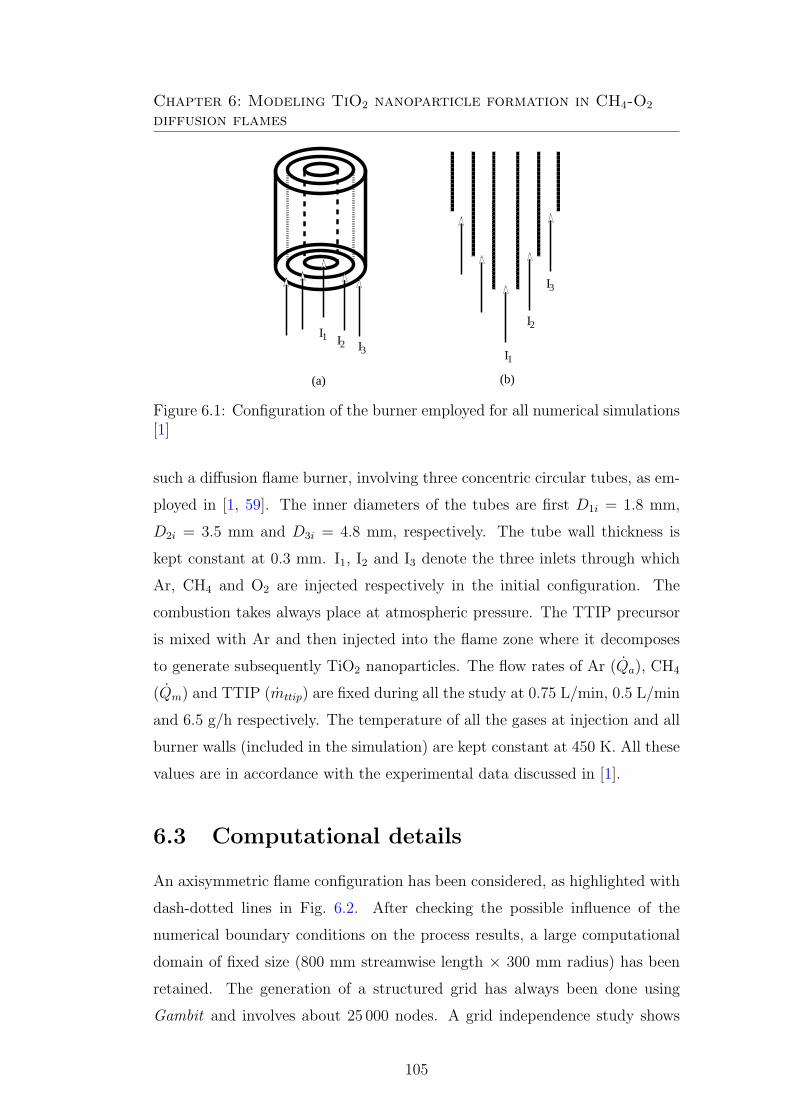
Chapter 6: Modeling TiO2 nanoparticle formation in CH4-O2
diffusion flames
I
I
I
(a) (b)
II I
�����������������������������������
�����������������������������������
�����������������������������������
�����������������������������������
������������������������������������������������������
������������������������������������������������������
���������������
���������������
���������������
���������������
������������������������������������������������������
������������������������������������������������������
1
2
3
12
3
Figure 6.1: Configuration of the burner employed for all numerical simulations[1]
such a diffusion flame burner, involving three concentric circular tubes, as em-
ployed in [1, 59]. The inner diameters of the tubes are first D1i = 1.8 mm,
D2i = 3.5 mm and D3i = 4.8 mm, respectively. The tube wall thickness is
kept constant at 0.3 mm. I1, I2 and I3 denote the three inlets through which
Ar, CH4 and O2 are injected respectively in the initial configuration. The
combustion takes always place at atmospheric pressure. The TTIP precursor
is mixed with Ar and then injected into the flame zone where it decomposes
to generate subsequently TiO2 nanoparticles. The flow rates of Ar (Qa), CH4
(Qm) and TTIP (mttip) are fixed during all the study at 0.75 L/min, 0.5 L/min
and 6.5 g/h respectively. The temperature of all the gases at injection and all
burner walls (included in the simulation) are kept constant at 450 K. All these
values are in accordance with the experimental data discussed in [1].
6.3 Computational details
An axisymmetric flame configuration has been considered, as highlighted with
dash-dotted lines in Fig. 6.2. After checking the possible influence of the
numerical boundary conditions on the process results, a large computational
domain of fixed size (800 mm streamwise length × 300 mm radius) has been
retained. The generation of a structured grid has always been done using
Gambit and involves about 25 000 nodes. A grid independence study shows
105
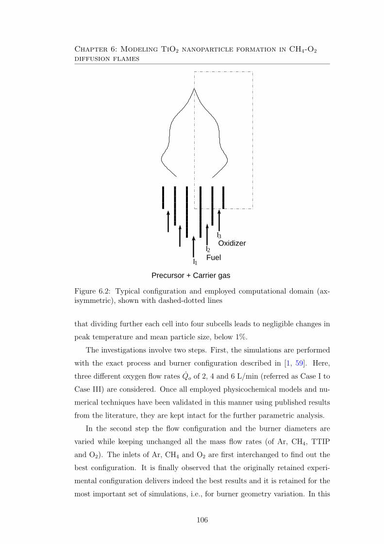
Chapter 6: Modeling TiO2 nanoparticle formation in CH4-O2
diffusion flames
I
I
I������������������������������������
������������������������������������
��������������
��������������
������������������������������������
������������������������������������
����������������������������
����������������������������
��������
��������
��������
��������
1
2
3Oxidizer
Fuel
Precursor + Carrier gas
Figure 6.2: Typical configuration and employed computational domain (ax-isymmetric), shown with dashed-dotted lines
that dividing further each cell into four subcells leads to negligible changes in
peak temperature and mean particle size, below 1%.
The investigations involve two steps. First, the simulations are performed
with the exact process and burner configuration described in [1, 59]. Here,
three different oxygen flow rates Qo of 2, 4 and 6 L/min (referred as Case I to
Case III) are considered. Once all employed physicochemical models and nu-
merical techniques have been validated in this manner using published results
from the literature, they are kept intact for the further parametric analysis.
In the second step the flow configuration and the burner diameters are
varied while keeping unchanged all the mass flow rates (of Ar, CH4, TTIP
and O2). The inlets of Ar, CH4 and O2 are first interchanged to find out the
best configuration. It is finally observed that the originally retained experi-
mental configuration delivers indeed the best results and it is retained for the
most important set of simulations, i.e., for burner geometry variation. In this
106

Chapter 6: Modeling TiO2 nanoparticle formation in CH4-O2
diffusion flames
third and last part, the internal diameters of the 3 burners (D1i, D2i, D3i)
are systematically varied (increased or decreased) by ± 10% or ± 20%. Con-
sidering construction constraints, this finally delivers twelve different burner
geometries.
Then, the properties of the obtained flames are investigated. Out of the
twelve configurations, the six cases leading to stable combustion are gathered
in Table 6.1 along with the corresponding burner dimensions. Please note that
in this table a superscript of 10 or 20 indicates an increase in inner diameter by
10 or 20%, while a subscript of 10 or 20 indicates a decrease in inner diameter
by 10 or 20%. Hereafter these cases are systematically referred to as Case 1 to
Case 6. Once the resulting flame fields have been determined, the computation
of the PSD can be started, as described later. For one configuration, the typical
computational time using 8 computing cores of a Linux-based PC cluster in
parallel is approximately 16 hours.
Table 6.1: Configurations finally considered during the numerical simulationsince they can be constructed and lead to stable combustion (Note: superscript10 and subscript 10 indicates (+) and (-) 10% change from the initial innerdiameters listed in the first line; similarly for 20). The corresponding injectionvelocities (in m/s) are given in the last three columns
Case Description D1i D2i D3i v1i (Ar) v2i (CH4) v3i (O2)Initial D1iD2iD3i 1.80 3.50 4.80 4.91 1.63 6.81Case 1 D1i10D2i10D3i10 1.98 3.85 5.28 4.06 1.29 5.25Case 2 D1i10D2i10D3i10 1.98 3.15 5.28 4.06 3.25 3.07Case 3 D1i10D2i10D3i10 1.62 3.85 5.28 6.06 1.07 5.25Case 4 D1i20D2i20D3i20 1.44 4.20 5.76 7.67 0.78 4.18Case 5 D1i20D2i20D3i20 1.44 2.80 5.76 7.67 2.88 1.96Case 6 D1i20D2i20D3i20 1.44 2.80 3.84 7.67 2.88 13.31
6.4 Employed models
The industrial CFD solver Ansys-Fluent has been again used to solve the gas-
phase governing equations, considering a detailed CH4-O2 combustion mecha-
nism with 17 species and 41 reactions. The turbulence is still modeled with the
standard k− ǫ model. The Eddy Dissipation Concept (EDC) model is used to
handle the turbulence-chemistry interactions, which is different from our ear-
107
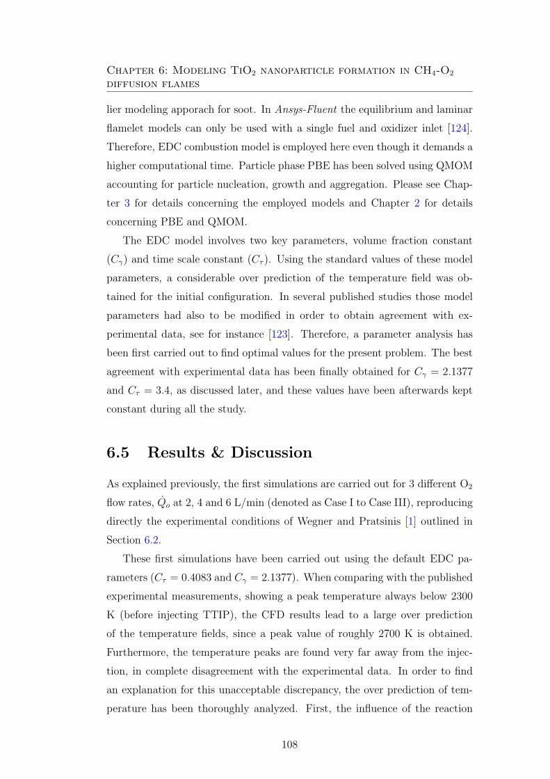
Chapter 6: Modeling TiO2 nanoparticle formation in CH4-O2
diffusion flames
lier modeling apporach for soot. In Ansys-Fluent the equilibrium and laminar
flamelet models can only be used with a single fuel and oxidizer inlet [124].
Therefore, EDC combustion model is employed here even though it demands a
higher computational time. Particle phase PBE has been solved using QMOM
accounting for particle nucleation, growth and aggregation. Please see Chap-
ter 3 for details concerning the employed models and Chapter 2 for details
concerning PBE and QMOM.
The EDC model involves two key parameters, volume fraction constant
(Cγ) and time scale constant (Cτ ). Using the standard values of these model
parameters, a considerable over prediction of the temperature field was ob-
tained for the initial configuration. In several published studies those model
parameters had also to be modified in order to obtain agreement with ex-
perimental data, see for instance [123]. Therefore, a parameter analysis has
been first carried out to find optimal values for the present problem. The best
agreement with experimental data has been finally obtained for Cγ = 2.1377
and Cτ = 3.4, as discussed later, and these values have been afterwards kept
constant during all the study.
6.5 Results & Discussion
As explained previously, the first simulations are carried out for 3 different O2
flow rates, Qo at 2, 4 and 6 L/min (denoted as Case I to Case III), reproducing
directly the experimental conditions of Wegner and Pratsinis [1] outlined in
Section 6.2.
These first simulations have been carried out using the default EDC pa-
rameters (Cτ = 0.4083 and Cγ = 2.1377). When comparing with the published
experimental measurements, showing a peak temperature always below 2300
K (before injecting TTIP), the CFD results lead to a large over prediction
of the temperature fields, since a peak value of roughly 2700 K is obtained.
Furthermore, the temperature peaks are found very far away from the injec-
tion, in complete disagreement with the experimental data. In order to find
an explanation for this unacceptable discrepancy, the over prediction of tem-
perature has been thoroughly analyzed. First, the influence of the reaction
108
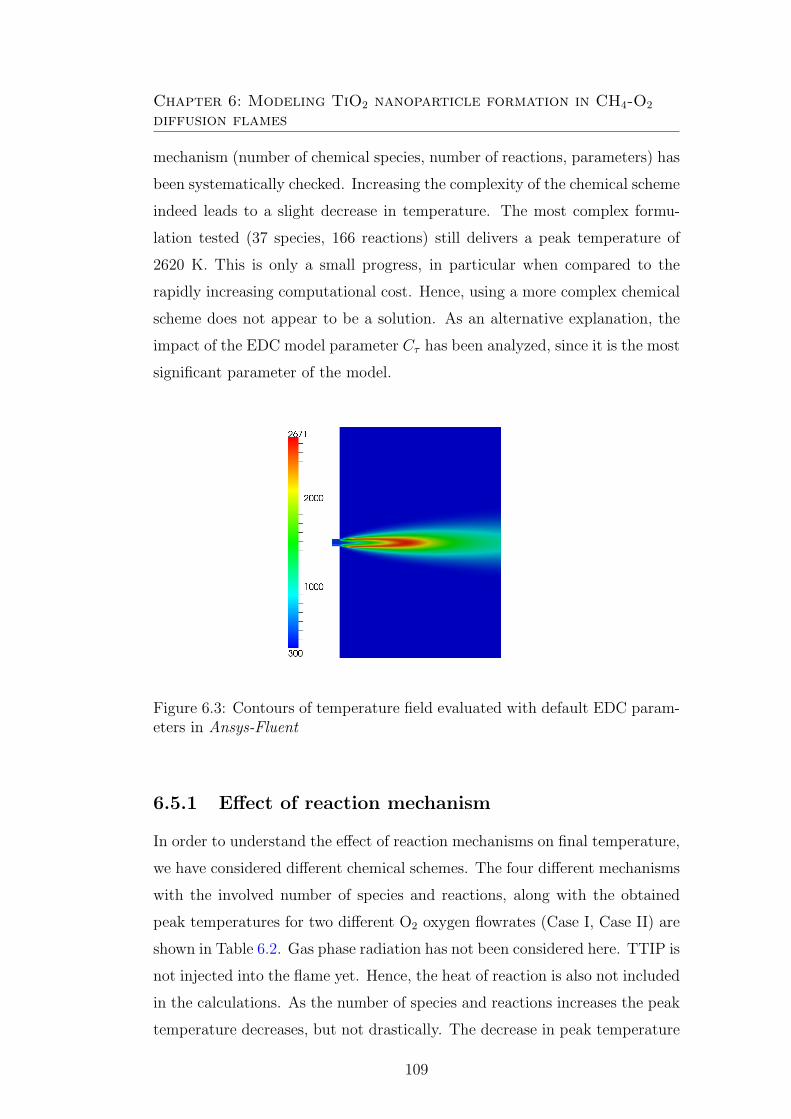
Chapter 6: Modeling TiO2 nanoparticle formation in CH4-O2
diffusion flames
mechanism (number of chemical species, number of reactions, parameters) has
been systematically checked. Increasing the complexity of the chemical scheme
indeed leads to a slight decrease in temperature. The most complex formu-
lation tested (37 species, 166 reactions) still delivers a peak temperature of
2620 K. This is only a small progress, in particular when compared to the
rapidly increasing computational cost. Hence, using a more complex chemical
scheme does not appear to be a solution. As an alternative explanation, the
impact of the EDC model parameter Cτ has been analyzed, since it is the most
significant parameter of the model.
Figure 6.3: Contours of temperature field evaluated with default EDC param-eters in Ansys-Fluent
6.5.1 Effect of reaction mechanism
In order to understand the effect of reaction mechanisms on final temperature,
we have considered different chemical schemes. The four different mechanisms
with the involved number of species and reactions, along with the obtained
peak temperatures for two different O2 oxygen flowrates (Case I, Case II) are
shown in Table 6.2. Gas phase radiation has not been considered here. TTIP is
not injected into the flame yet. Hence, the heat of reaction is also not included
in the calculations. As the number of species and reactions increases the peak
temperature decreases, but not drastically. The decrease in peak temperature
109
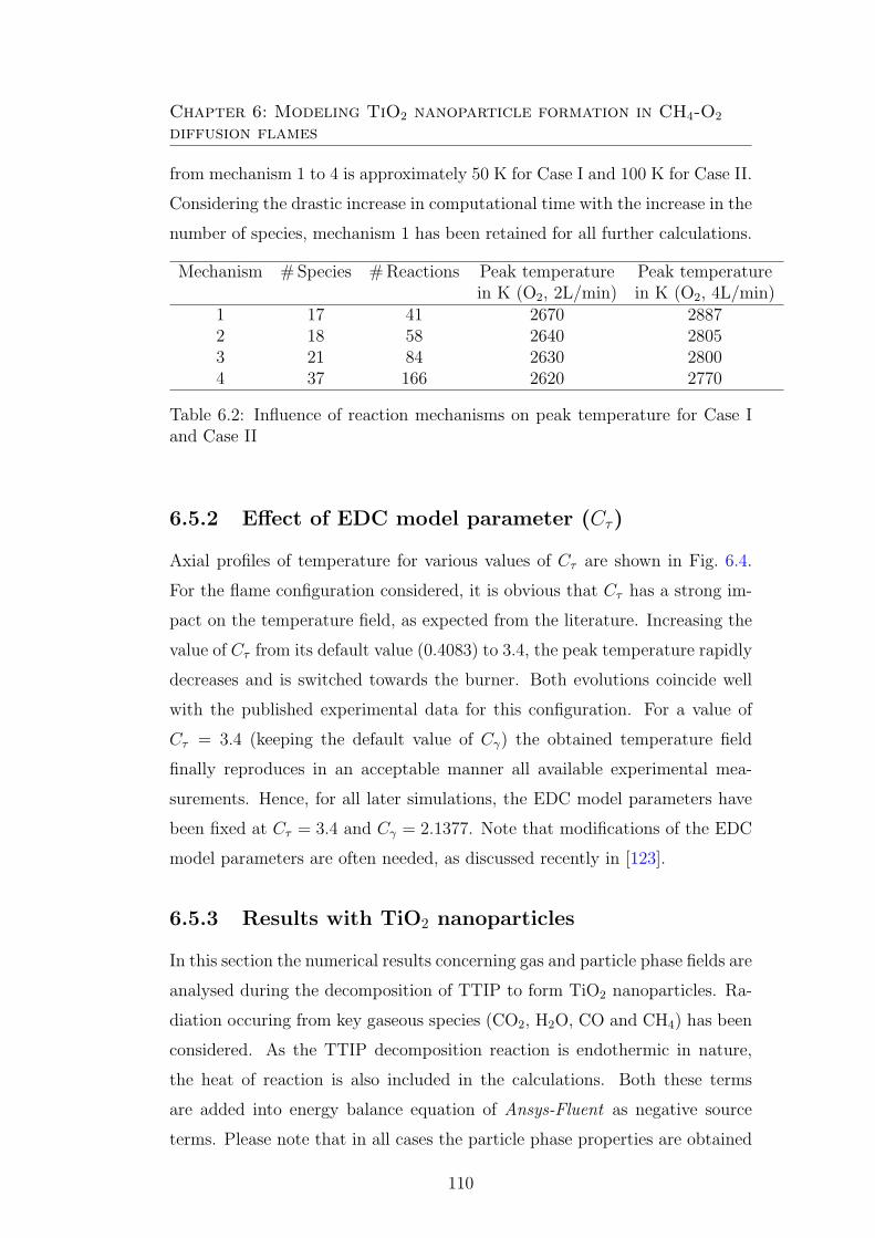
Chapter 6: Modeling TiO2 nanoparticle formation in CH4-O2
diffusion flames
from mechanism 1 to 4 is approximately 50 K for Case I and 100 K for Case II.
Considering the drastic increase in computational time with the increase in the
number of species, mechanism 1 has been retained for all further calculations.
Mechanism #Species #Reactions Peak temperature Peak temperaturein K (O2, 2L/min) in K (O2, 4L/min)
1 17 41 2670 28872 18 58 2640 28053 21 84 2630 28004 37 166 2620 2770
Table 6.2: Influence of reaction mechanisms on peak temperature for Case Iand Case II
6.5.2 Effect of EDC model parameter (Cτ)
Axial profiles of temperature for various values of Cτ are shown in Fig. 6.4.
For the flame configuration considered, it is obvious that Cτ has a strong im-
pact on the temperature field, as expected from the literature. Increasing the
value of Cτ from its default value (0.4083) to 3.4, the peak temperature rapidly
decreases and is switched towards the burner. Both evolutions coincide well
with the published experimental data for this configuration. For a value of
Cτ = 3.4 (keeping the default value of Cγ) the obtained temperature field
finally reproduces in an acceptable manner all available experimental mea-
surements. Hence, for all later simulations, the EDC model parameters have
been fixed at Cτ = 3.4 and Cγ = 2.1377. Note that modifications of the EDC
model parameters are often needed, as discussed recently in [123].
6.5.3 Results with TiO2 nanoparticles
In this section the numerical results concerning gas and particle phase fields are
analysed during the decomposition of TTIP to form TiO2 nanoparticles. Ra-
diation occuring from key gaseous species (CO2, H2O, CO and CH4) has been
considered. As the TTIP decomposition reaction is endothermic in nature,
the heat of reaction is also included in the calculations. Both these terms
are added into energy balance equation of Ansys-Fluent as negative source
terms. Please note that in all cases the particle phase properties are obtained
110

Chapter 6: Modeling TiO2 nanoparticle formation in CH4-O2
diffusion flames
0 0.02 0.04 0.06 0.08 0.1 0.12Axial position (m)
400
800
1200
1600
2000
2400
2800
T (
K)
Cτ=0.4083Cτ=1.0Cτ=2.0 Cτ=3.0Cτ=3.4
Figure 6.4: Axial profiles of temperature (in K) for various values of Cτ withreaction mechanism 1.
through Quadrature Method of Moments (QMOM) with 2 quadrature nodes.
DQMOM was not retained here due to stability issues.
Figure 6.5 now shows the obtained profiles of temperature (a)-(c), TTIP
concentration (d)-(f) and TiO2 concentration (g)-(i) for Case I, Case II and
Case III respectively. Due to lower O2 flow rate in Case I the mixing of
fuel/oxidizer is poor. As a result the temperature fields and consequently the
overall decomposition rate of TTIP extend far from the burner (see Figs.(a)
and (d)). Whereas, the decomposition is faster and closer to the burner in
Case III as temperature is higher near the burner (see Figs.(c) and (f)). The
same behavior is observed for TiO2. Figures 6.5 (g), (h) and (i) show the
contour plots of overall titania molar concentrations for the 3 different oxygen
flow rates. As the oxygen flow rates increase, the decomposition of TTIP
shifts towards the burner, subsequently TiO2 production also shifts towards
the burner. Please note that the particle phase PBE solver (QMOM) is not
activated yet. For Case I (Fig. 6.5 (g)) and Case II (Fig. 6.5 (h)) the overall
TiO2 formation is higher than that of Case III (Fig. 6.5 (i)). Once the TiO2
molar concentration is known, corresponding nucleation and surface growth
terms can be evaluated from Eq. (3.25) and Eq. (3.26), respectively. In the
case of nucleation a uniform distribution of particles in the particle volume
range 0 ≤ ξ ≤ ε (ξ being the internal co-ordinate, in this case particle volume)
111
Chapter 6: Modeling TiO2 nanoparticle formation in CH4-O2
diffusion flames
has been considered. For the present case, ε is assumed to be 1 nm3, a little
higher than the volume of a TiO2 monomer (≈ 0.0332 nm3). Nucleation
forms a uniform distribution of particles in the particle volume range [0, 1] nm3
(please see Chapter 2 for a detailed description).
Figure 6.6 shows the corresponding comparison of axial profiles of tem-
perature with experimental data for two different O2 flow rates (Case II and
Case III), since no experimental data is available for Case I. Please note that,
the gas radiation from the key species and the heat of reaction for TTIP de-
composition have been included in the simulations. As the flow rate of O2
increases, the peak temperatures are reduced and shifted towards the burner,
due to a faster mixing induced by higher turbulence levels. The temperature
profiles predicted by simulation are slightly lower and shifted away from the
burner when compared to the experimental data. However, the comparison is
quite fair and the changes between Case II and Case III are very well repro-
duced by CFD.
6.6 Parametric study
Obtaining as far as possible a monodisperse distribution of nanoparticles with
a low diameter and in a large quantity would be very desirable for practical
applications. Hence, the influence of different parameters is now considered in
order to achieve the best possible conditions: minimize dmean, maximize fv,
and minimize σg (the width of the distribution), if possible simultaneously.
6.6.1 Exchanging injections for a fixed geometry
In a first step, we have tried interchanging systematically the gas injections
(Ar, CH4 and O2) within the three available tubes (Inlet I1, I2, I3, shown in
Table 6.3), all other parameters between fixed. After computing all configu-
rations, it appeared that the initial configuration (inlet I1: Ar, Inlet I2: CH4,
Inlet I3: O2) is the only one leading to a stable flame. In all other cases, it
was either impossible to start the combustion or to stabilize the flame.
112

Chapter 6: Modeling TiO2 nanoparticle formation in CH4-O2
diffusion flames
Config.No. Inlet-I1 Inlet-I2 Inlet-I31 CH4 O2 Ar2 CH4 Ar O2
3 O2 CH4 Ar4 O2 Ar CH4
5 Ar CH4 O2
6 Ar O2 CH4
Table 6.3: Different configurations considered in the numerical simulation tostudy the impact on the PSD
6.6.2 Effect of change in burner diameter
Keeping now these injections and all mass flow rates constant, the burner
geometry has been systematically varied by increasing or decreasing the inner
diameters by 10 or 20%. The results for Case 1 to Case 6 (already presented
in Table 6.1, on page 107) are now analyzed in detail.
Figure 6.7 shows all corresponding temperature profiles along the burner
axis. The simulation data for the initial configuration is shown with a solid
curve, while different symbols are used for Case 1 to Case 6. As seen in the
figure, even with fixed mass flow rates and injections, considerable differences
are observed in the obtained temperature fields, both in terms of peak value
and of spatial distribution. The peak values range from ≈ 1900 K for Case 6
to ≈ 2300 K for Case 5. These differences are best seen in the inset plot in
the top-right corner. The slopes and width of the high temperature regions
differ as well. For instance, Case 6 shows only a short span with high temper-
atures compared to Case 5. When compared to the initial configuration (solid
curve) the obtained differences are as expected more significant for Cases 4, 5
and 6 (variations of internal diameters by ± 20%), while differences are less
pronounced for Cases 1, 2 and 3 (variations of diameters by only ± 10%).
Since it is known from the literature that process temperature is the most
significant parameter to control particle properties, large variations are now
expected concerning the PSD of produced TiO2 particles.
Axial profiles of TiO2 molar concentration in gas phase are depicted in
Fig. 6.8. The injection velocities are highest for Case 6, hence the temperatures
and correspondingly TTIP decomposition and TiO2 conversion are higher close
113
Chapter 6: Modeling TiO2 nanoparticle formation in CH4-O2
diffusion flames
to the burner. In contrast, for Case 2, the injection velocities are very low,
inducing low turbulence (see Table 6.1 for the injection velocities). Therefore,
the peak value is shifted away from the burner.
Figure 6.9 shows the obtained profiles of volume fraction fv along the
central axis of the burner. The peak volume fraction is maximum for Case 1,
slightly higher than for the initial configuration, and minimum for Case 5.
In spite of its lowest peak temperature, Case 6 also leads to a high peak
in volume fraction (≈ 6.5 ppm), illustrating the complexity of the coupled
physicochemical processes controlling particle formation. As already discussed
for flame temperature, an increase in injection velocities (decrease in injection
slot diameter) leads to a shift of all quantities (temperature, TTIP, TiO2)
towards the burner (compare Case 6, where all profiles reach peak values close
to the burner, to Case 2 for which the evolutions are delayed). To summarize
concerning TiO2 molar concentration and peak volume fraction, the highest
values are observed for Case 1, initial configuration, and Case 6, in decreasing
order.
One major particle quantity of interest is the mean diameter, dmean of the
TiO2 nanoparticles. Figure 6.10 shows dmean along the burner central axis for
all cases. At first, dmean increases rapidly close to the burner, it then decreases
before increasing again gradually until the end of the computational domain.
This complex evolution is a consequence of the competition between nucle-
ation, growth and aggregation. When looking in details at the source terms
of the moment transport equations and at the corresponding rate equations
(kg, ks and β), two separate regions (one directly behind the burner, one con-
siderably further downstream) are found with intense nucleation. After the
first nucleation burst, the nanoparticle diameter increases rapidly due to ag-
gregation. After reaching its peak mean diameter, the impact of aggregation
decreases and molecular growth dominates, until reaching the second region
of nucleation. Later, the mean particle size increases gradually till the end of
the computational domain due to aggregation. As a whole, it is observed that
the largest particles are produced for Case 2, where the injection velocities
are smaller leading to slow evolutions. The smallest mean diameter dmean is
obtained for Case 6 where the injection velocities are large, leading to very
114

Chapter 6: Modeling TiO2 nanoparticle formation in CH4-O2
diffusion flames
fast evolutions directly after injection. The initial configuration is once again
second best, this time after Case 6, concerning dmean.
The standard deviation (σg) quantifying the width of the PSD is shown in
Fig. 6.11. It is seen in this picture that all cases produce the same qualitative
trend. σg increases rapidly up to about 2.3 close to the inlet, then drops rapidly
to ≈ 1.3. This indicates again that, as soon as the particles are formed, they
rapidly grow due to aggregation, broadening the PSD (σg → 2.3). Following
this phase, with mostly nucleation and very little effect from molecular growth
and aggregation, a value of σg close to 1.3 is obtained, indicating a nearly
monodisperse distribution in this region. Later on, σg gradually increases
again, goes through a smaller secondary peak, then slowly decreases before
reaching finally a nearly constant value in the range ≈ 1.5− 1.7. Considering
that σg should be minimized, the initial configuration and Case 1 are now the
worst cases, while Case 3 and Case 4 deliver optimal conditions.
The peak values of temperature, of dmean, of fv and the value of σg at
the outlet are presented for all Cases in Table 6.4. Remembering that the
objective was to minimize dmean, maximize fv and minimize σg, the best three
cases are associated in this Table respectively with +++ (best), ++ (second
best) and + (third best). Similarly, the three worst cases are associated with
− − −/ − −/−. Case 6 shows the lowest peak temperature and leads to
nanoparticles with the lowest mean diameter dmean (46.6 nm), together with
a high volume fraction (fv ≈ 6.4 ppm). When compared to the initial burner
configuration the geometric standard deviation at the outlet is also less (1.61)
for Case 6, compared to 1.66 for the initial configuration. Case 1 leads to the
highest volume fraction (fv ≈ 6.4 ppm), which is positive, but unfortunately
also to the largest standard deviation.
Looking again at Table 6.4, it is difficult to identify a clear winner for
all three objectives. Indeed, the analysis confirms the quality of the original
experimental work, since the initial configuration belongs to the very best
in terms of volume fraction and particle diameter. However, it is the worst
one concerning the width of the PSD. This negative correlation appears to
be a general rule. Hence, future analysis will have to consider a concurrent
optimization process, since the objectives cannot be fulfilled simultaneously.
115
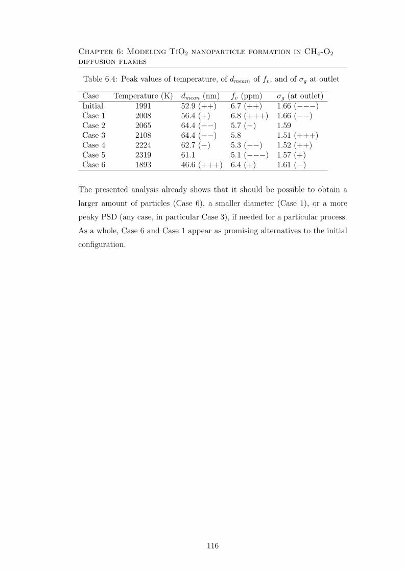
Chapter 6: Modeling TiO2 nanoparticle formation in CH4-O2
diffusion flames
Table 6.4: Peak values of temperature, of dmean, of fv, and of σg at outlet
Case Temperature (K) dmean (nm) fv (ppm) σg (at outlet)Initial 1991 52.9 (++) 6.7 (++) 1.66 (−−−)Case 1 2008 56.4 (+) 6.8 (+++) 1.66 (−−)Case 2 2065 64.4 (−−) 5.7 (−) 1.59Case 3 2108 64.4 (−−) 5.8 1.51 (+++)Case 4 2224 62.7 (−) 5.3 (−−) 1.52 (++)Case 5 2319 61.1 5.1 (−−−) 1.57 (+)Case 6 1893 46.6 (+++) 6.4 (+) 1.61 (−)
The presented analysis already shows that it should be possible to obtain a
larger amount of particles (Case 6), a smaller diameter (Case 1), or a more
peaky PSD (any case, in particular Case 3), if needed for a particular process.
As a whole, Case 6 and Case 1 appear as promising alternatives to the initial
configuration.
116

Chapter 6: Modeling TiO2 nanoparticle formation in CH4-O2
diffusion flames
(a) (b) (c)
(d) (e) (f)
(g) (h) (i)
Figure 6.5: Contour plots of temperature (a, b, c) in K, TTIP (d, e, f) andTiO2 (g, h, i) concentrations in mol/m3 for Case I, Case II and Case III (fromleft to right). The same color scale is employed for all three Cases.
117
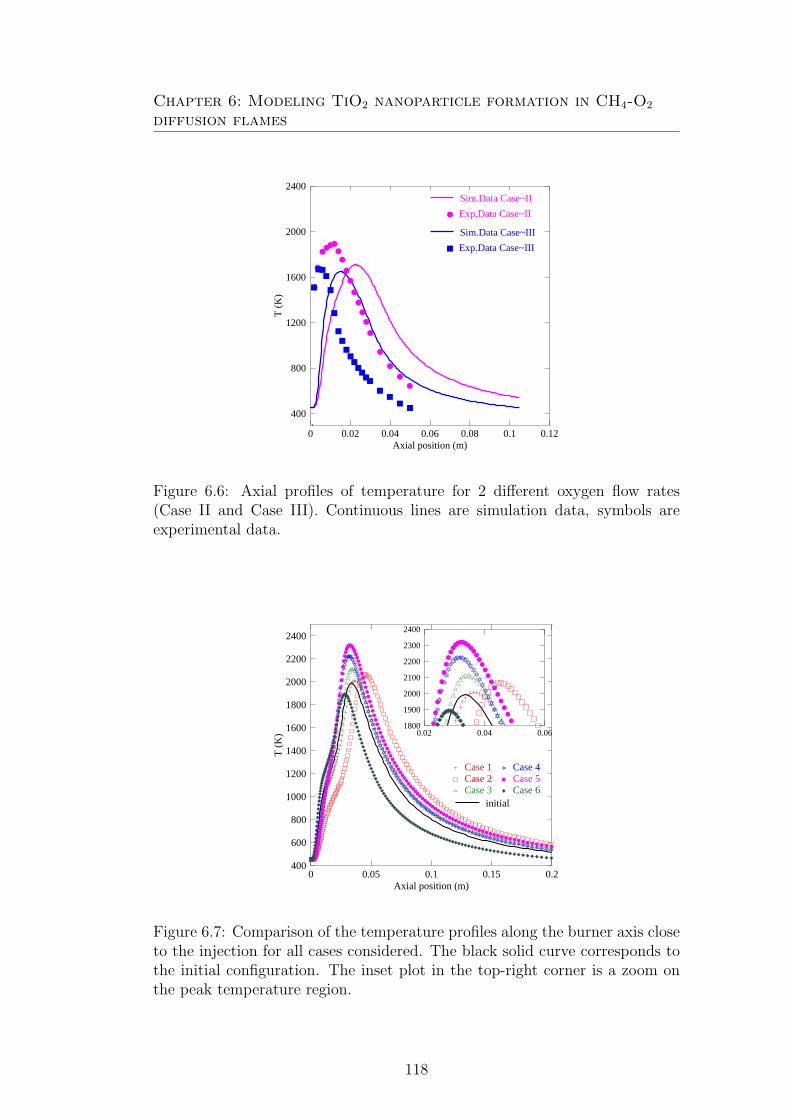
Chapter 6: Modeling TiO2 nanoparticle formation in CH4-O2
diffusion flames
0 0.02 0.04 0.06 0.08 0.1 0.12Axial position (m)
400
800
1200
1600
2000
2400
T (
K)
Sim.Data Case~II
Exp.Data Case~II
Sim.Data Case~III
Exp.Data Case~III
Figure 6.6: Axial profiles of temperature for 2 different oxygen flow rates(Case II and Case III). Continuous lines are simulation data, symbols areexperimental data.
0 0.05 0.1 0.15 0.2Axial position (m)
400
600
800
1000
1200
1400
1600
1800
2000
2200
2400
T (
K)
Case 1Case 2Case 3
Case 4Case 5Case 6
initial
0.02 0.04 0.061800
1900
2000
2100
2200
2300
2400
Figure 6.7: Comparison of the temperature profiles along the burner axis closeto the injection for all cases considered. The black solid curve corresponds tothe initial configuration. The inset plot in the top-right corner is a zoom onthe peak temperature region.
118

Chapter 6: Modeling TiO2 nanoparticle formation in CH4-O2
diffusion flames
0 0.05 0.1 0.15 0.2Axial position (m)
0
0.1
0.2
0.3
0.4
TiO
2 (g
mol
/m3)
Case 1
Case 2
Case 3
Case 4
Case 5
Case 6
initial
0.01 0.02 0.03 0.04 0.050.25
0.3
0.35
Figure 6.8: Comparison of the profiles of TiO2 concentration (in gmol/m3)along the flame axis for all the cases considered. Black solid curve is withoriginal configuration.
0 0.05 0.1 0.15 0.2Axial position (m)
0
2
4
6
8
Vol
ume
frac
tion
of T
iO2
(µ1)
Case 1
Case 2
Case 3
Case 4
Case 5
Case 6
initial
0.01 0.02 0.03 0.04 0.054
5
6
7
Figure 6.9: Comparison of the volume fraction profiles of TiO2 (fv, in ppm)along the burner axis close to the injection for all cases considered.
119

Chapter 6: Modeling TiO2 nanoparticle formation in CH4-O2
diffusion flames
0 0.05 0.1 0.15 0.2Axial position (m)
0
10
20
30
40
50
60
70
d mea
n (n
m)
Case 1
Case 2
Case 3
Case 4
Case 5
Case 6
initial
Figure 6.10: Comparison of the profiles of mean particle diameter (dmean, innm) along the burner axis close to the injection for all cases considered.
0 0.05 0.1 0.15 0.2Axial position (m)
1
1.5
2
2.5
σ g
Case 1
Case 2
Case 3
Case 4
Case 5
Case 6
initial
Figure 6.11: Comparison of the profiles of standard deviation (σg) along theburner axis close to the injection for all cases considered.
120
Chapter 7
Conclusions
The first objective of the present study was to develop an improved soot pre-
diction model for turbulent non-premixed ethylene/air flames. Optimization
relying on Genetic Algorithms coupled with evaluations of the solution by
CFD coupled with DQMOM have been carried out for this purpose. The
two objective functions of the optimization problem are the absolute differ-
ences concerning temperature (T ) and soot volume fraction (fv) as obtained
by CFD and by published experiments. A sensitivity analysis revealed that
the three main parameters describing the evolution of the soot particles are
the activation temperature of nucleation Tn and of oxidation To, together with
radiation constant C0. They have therefore been chosen as parameters of the
first optimization. The optimal parameter set identified by the procedure leads
indeed to a considerable improvement for the target flame [50].
The generality of the optimal set of parameters has then been further tested
by comparison with three additional flames, investigated experimentally in the
literature. The results show a systematic improvement concerning the most
important value for practical applications, i.e., the peak soot volume fraction.
The temperature fields are also always improved. Nevertheless, even if the
form of the axial profile for soot volume fraction also improves, it is however
simultaneously shifted towards the burner.
To solve this undesirable shift, turbulence/chemistry coupling has been de-
scribed in the final optimization step using a more accurate flamelet model.
Optimization considering four model parameters of the particulate phase (in
the final step, activation temperature of nucleation Tn, of oxidation To, of
121

Chapter 7: Conclusions
particle growth Tg and radiation constant C0) and two concurrent objective
functions (for T and fv evaluated similar to the earlier case) has been carried
out successfully. The optimal parameter set finally identified by the proce-
dure leads to a considerable improvement for all measured quantities. After
optimization, the generality of the obtained models has been checked by com-
puting further separate flames. A very good agreement is obtained for all
cases, both for axial and radial profiles. As a consequence, the model combi-
nation presented in this work appears to be generally suitable for predicting
soot formation in turbulent non-premixed ethylene/air flames.
Due to the tight coupling of soot particulate models with temperature it
is necessary to take into account in a suitable manner radiative heat transfer.
When computational costs are important, for instance when considering prac-
tical burners, only very simple models can be employed to describe radiation.
In the present study, three such models have been considered. The importance
of gas (CO2 and H2O) and soot radiation has been first shown. Using already
optimized soot particulate models, the best possible radiation proportionality
constant (C0, C1 and C2) have been determined. The generality of the results
has been checked. Unfortunately, it is observed that the previously employed
Radiation model I can not be beaten by the alternative models II and III.
All three models, being very similar in their structure, finally lead almost to
the same optimum for the conditions considered here. Therefore, it appears
that noticeable progress would only be possible by considering much more
complex (and numerically expensive) models to describe radiative heat loss,
since grey gas and optically thin approximation obviously constitute a major
simplification of the true physics.
A numerical analysis of TiO2 nanoparticle production has been carried
out in the second part of this work, considering CH4-O2 diffusion flames with
TTIP as precursor. Different combinations of flow configurations and burner
geometries have been tested with the aim of obtaining nanoparticles with de-
sired properties (minimum diameter dmean, maximum volume fraction fv and
minimum width of the PSD σg). A detailed gas phase chemistry is taken
into account with 17 species and 41 reactions. The EDC combustion model is
used to handle turbulence-chemistry interaction. Aerosol evolution is tracked
122

Chapter 7: Conclusions
with a population balance equation taking into account nucleation, molecular
growth and aggregation. The Quadrature Method of Moments is used with two
quadrature nodes to solve the PBE. Gas radiation and heat of reaction of TTIP
decomposition have been taken into account. Initial test results performed for
three different O2 flow rates have been used to validate against experimental
data from literature, adapting the EDC model parameters. Then, an opti-
mal configuration is searched for, first by interchanging the fuel, oxidizer and
carrier gas inlets. The initial configuration is found to be the most suitable
to produce a stable flame. Selecting then this flow configuration and fixing
the mass flow rates of CH4, O2, Ar and TTIP, geometric variations have been
considered by increasing/decreasing the internal diameters (D1i, D2i and D3i)
of the diffusion burner by up to ± 20%. The numerical results carried out
in 6 cases (Case 1 to Case 6) show a significant difference in temperatures,
and therefore also in resulting particle properties. Case 1, initial configuration
and Case 6 produce highest TiO2 nanoparticle volume fraction, whereas mean
particle diameter (dmean) is lowest for Case 6. In the future, an automatic and
concurrent optimization should be carried out in order to refine the analysis
and to identify even better configuration.
123

Bibliography
[1] K. Wegner and S. E. Pratsinis, “Nozzle-quenching process for controlled
flame synthesis of titania nanoparticles,” AIChE Journal, vol. 49, no. 7,
pp. 1667–1675, 2003.
[2] D. B. Kittelson, “Engines and nanoparticles: a review,” Journal of
Aerosol Science, vol. 29, no. 5-6, pp. 575–588, 1998.
[3] T. C. Bond, “Black carbon: Emission sources and prioritization,” in
International Workshop on Black Carbon, London, UK, 2009.
[4] E. Auer, A. Freund, J. Pietsch, and T. Tacke, “Carbons as supports
for industrial precious metal catalysts,” Applied Catalysis A: General,
vol. 173, no. 2, pp. 259–271, 1998.
[5] UNEP and WMO, “Integrated assessment of black carbon and tropo-
spheric ozone summary for decision makers,” Report: Integrated Assess-
ment of Black Carbon and Tropospheric Ozone: Summary for Decision
Makers, 2011.
[6] V. Ramanathan, “Non-CO2 emissions: Options for a way forward,”
Black Carbon e-Bulletin, vol. 1, pp. 1–4, July 2009.
[7] V. Ramanathan, “Black carbon & India.” Environmental Ministry Meet-
ing, New Delhi, India, Oct 2009.
[8] H. Wang, “Formation of nascent soot and other condensed-phase mate-
rials in flames,” Proceedings of the Combustion Institute, vol. 33, no. 1,
pp. 41–67, 2011.
124

Bibliography
[9] J. P. Cain, J. Camacho, D. J. Phares, H. Wang, and A. Laskin, “Evidence
of aliphatics in nascent soot particles in premixed ethylene flames,” Pro-
ceedings of the Combustion Institute, vol. 33, no. 1, pp. 533–540, 2011.
[10] D. Thevenin and G. Janiga, Optimization and Computational Fluid Dy-
namics. Springer, 2008.
[11] R. Hilbert, G. Janiga, R. Baron, and D. Thevenin, “Multi-objective
shape optimization of a heat exchanger using parallel genetic algo-
rithms,” International Journal of Heat and Mass Transfer, vol. 49,
pp. 2567–2577, 2006.
[12] G. Janiga and D. Thevenin, “Reducing the CO emissions in a lami-
nar burner using different numerical optimization methods,” Journal of
Power and Energy, vol. 221, pp. 647–655, 2007.
[13] W. Stober and U. R. Abel, “Lung cancer due to diesel soot particles in
ambient air?,” International Archives of Occupational and Environmen-
tal Health, vol. 68, pp. 3–61, 1996.
[14] J. J. Sauvain, T. V. Duc, and M. Guillemin, “Exposure to carcinogenic
polycyclic aromatic compounds and health risk assessment for diesel-
exhaust exposed workers,” International Archives of Occupational and
Environmental Health, vol. 76, pp. 443–455, 2003.
[15] V. Ramanathan and G. Carmichael, “Global and regional climate
changes due to black carbon,” Nature Geoscience, vol. 1, pp. 221–227,
2008.
[16] S. Menon, J. Hansen, L. Nazarenko, and Y. Luo, “Climate effects of black
carbon aerosols in China and India,” Science, vol. 297, pp. 2250–2253,
2002.
[17] Y. J. Kaufman and I. Koren, “Smoke and pollution aerosol effect on
cloud cover,” Science, vol. 313, pp. 655–658, 2006.
125

Bibliography
[18] M. Frenklach and H. Wang, “Aromatics growth beyond the first ring
and the nucleation of soot particles,” tech. rep., Department of Materials
Science and Engineering, The Pennsylvania State University, 1991.
[19] H. Pitsch, E. Riesmeier, and N. Peters, “Unsteady flamelet modeling of
soot formation in turbulent diffusion flames,” Combustion Science and
Technology, vol. 158, no. 1, pp. 389–406, 2000.
[20] F. Mauss, K. Netzell, and H. Lehtiniemi, “Aspects of modeling soot
formation in turbulent diffusion flames,” Combustion Science and Tech-
nology, vol. 178, pp. 1871–1885, 2006.
[21] L. Wang, D. C. Haworth, S. R. Turns, and M. F. Modest, “Interactions
among soot, thermal radiation, and NOx emissions in oxygen-enriched
turbulent nonpremixed flames: a computational fluid dynamics modeling
study,” Combustion and Flame, vol. 141, pp. 170–179, 2005.
[22] J. Appel, H. Bockhorn, and M. Wulkow, “A detailed numerical study
of the evolution of soot particle size distributions in laminar premixed
flames,” Chemosphere, vol. 42, pp. 635–645, 2001.
[23] M. Balthasar, F. Mauss, M. Pfitzner, and A. Mack, “Implementation
and validation of a new soot model and application to aeroengine com-
bustors,” Journal of Engineering for Gas Turbines and Power, vol. 124,
no. 1, pp. 66–74, 2002.
[24] I. M. Aksit and J. B. Moss, “A hybrid scalar model for sooting turbulent
flames,” Combustion and Flame, vol. 145, pp. 231–244, 2006.
[25] D. O. Lignell, J. H. Chen, P. J. Smith, T. Lu, and C. K. Law, “The
effect of flame structure on soot formation and transport in turbulent
nonpremixed flames using direct numerical simulation,” Combustion and
Flame, vol. 151, pp. 2–28, 2007.
[26] G. Ma, J. Z. Wen, M. F. Lightstone, and M. J. Thomson, “Optimization
of soot modelling in turbulent non-premixed ethylene/air jet flames,”
Combustion Science and Technology, vol. 177, pp. 1567–1602, 2005.
126

Bibliography
[27] F. Tao, V. I. Golovitchev, and J. Chomiak, “A phenomenological model
for the prediction of soot formation in diesel spray combustion,” Com-
bustion and Flame, vol. 136, no. 3, pp. 270–282, 2004.
[28] B. S. Haynes and H. G. Wagner, “Soot formation,” Progress in Energy
and Combustion Science, vol. 7, pp. 229–273, 1981.
[29] H. Richter and J. B. Howard, “Formation of polycyclic aromatic hydro-
carbons and their growth to soot: a review of chemical reaction path-
ways,” Progress in Energy and Combustion Science, vol. 26, pp. 565–608,
2000.
[30] A. Zucca, D. L. Marchisio, A. A. Barresi, and R. O. Fox, “Implementa-
tion of the population balance equation in CFD codes for modelling soot
formation in turbulent flames,” Chemical Engineering Science, vol. 61,
pp. 87–95, 2006.
[31] H. El-Asrag and S. Menon, “Large eddy simulation of soot formation in
a turbulent non-premixed jet flame,” Combustion and Flame, vol. 156,
pp. 385–395, 2009.
[32] D. L. Marchisio and A. A. Barresi, “Investigation of soot formation in
turbulent flames with a pseudo-bivariate population balance model,”
Chemical Engineering Science, vol. 64, pp. 294–303, 2009.
[33] A. Oncul, H. El-Rabii, and D. Thevenin, “Prediction of soot formation
in non-premixed flames using DQMOM,” in International Conference on
Multiphase Flow, (Leipzig, Germany), pp. 67/1–67/7, 2007.
[34] R. Viskanta and M. P. Menguc, “Radiation heat transfer in combustion
systems,” Progress in Energy and Combustion Science, vol. 13, no. 2,
pp. 97–160, 1987.
[35] R. Siegel and J. R. Howell, Thermal Radiation Heat Transfer. Taylor
and Francis, 1992.
[36] L. Wang, M. F. Modest, D. C. Haworth, and S. R. Turns, “Model-
ing nongray gas-phase and soot radiation in luminous turbulent non-
127
Bibliography
premixed jet flames,” Combustion Theory and Modelling, vol. 9, pp. 479–
498, 2005.
[37] S. C. Lee and C. L. Tien, “Effect of soot shape on soot radiation,”
Journal of Quantitative Spectroscopy and Radiative Transfer, vol. 29,
pp. 259–265, 1983.
[38] R. Said, A. Garo, and R. Borghi, “Soot formation modeling for turbulent
flames,” Combustion and Flame, vol. 108, pp. 71–86, 1997.
[39] M. J. Zimberg, S. H. Frankel, J. P. Gore, and Y. R. Sivathanu, “A study
of coupled turbulent mixing, soot chemistry, and radiation effects using
the linear eddy model,” Combustion and Flame, vol. 113, pp. 454–469,
1998.
[40] J. F. Widmann, “Evaluation of the Planck mean absorption coefficients
for radiation transport through smoke,” Combustion Science and Tech-
nology, vol. 175, pp. 2299–2308, 2003.
[41] K. Netzell, H. Lehtiniemi, and F. Mauss, “Calculating the soot particle
size distribution function in turbulent diffusion flames using a sectional
method,” Proceedings of the Combustion Institute, vol. 31, pp. 667–674,
2007.
[42] J. Singh, M. Balthasar, M. Kraft, and W. Wagner, “Stochastic modeling
of soot particle size and age distributions in laminar premixed flames,”
Proceedings of the Combustion Institute, vol. 30, no. 1, pp. 1457–1465,
2005.
[43] M. Celnik, R. Patterson, M. Kraft, and W. Wagner, “Coupling a stochas-
tic soot population balance to gas-phase chemistry using operator split-
ting,” Combustion and Flame, vol. 148, no. 3, pp. 158–176, 2007.
[44] J. Etheridge, S. Mosbach, M. Kraft, H. Wu, and N. Collings, “Mod-
elling soot formation in a DISI engine,” Proceedings of the Combustion
Institute, vol. 33, no. 2, pp. 3159–3167, 2011.
128
Bibliography
[45] D. Grosschmidt, P. Habisreuther, and H. Bockhorn, “Calculation of the
size distribution function of soot particles in turbulent diffusion flames,”
Proceedings of the Combustion Institute, vol. 31, pp. 657–665, 2007.
[46] A. Kazakov and M. Frenklach, “Dynamic modeling of soot particle coag-
ulation and aggregation: Implementation with the method of moments
and application to high-pressure laminar premixed flames,” Combustion
and Flame, vol. 114, pp. 484–501, 1998.
[47] M. Balthasar and M. Frenklach, “Detailed kinetic modeling of soot ag-
gregate formation in laminar premixed flames,” Combustion and Flame,
vol. 140, pp. 130–145, 2005.
[48] R. McGraw, “Description of aerosol dynamics by the quadrature method
of moments,” Aerosol Science and Technology, vol. 27, pp. 255–265, 1997.
[49] D. L. Marchisio and R. O. Fox, “Solution of population balance equations
using the direct quadrature method of moments,” Journal of Aerosol
Science, vol. 36, pp. 43–73, 2005.
[50] B. Yang, B. Hu, and U. O. Koylu, “Mean soot volume fractions in turbu-
lent hydrocarbon flames: a comparison of sampling and laser measure-
ments,” Combustion Science and Technology, vol. 177, pp. 1603–1626,
2005.
[51] B. Yang and U. O. Koylu, “Detailed soot field in a turbulent non-
premixed ethylene/air flame from laser scattering and extinction exper-
iments,” Combustion and Flame, vol. 141, no. 3, pp. 55–65, 2005.
[52] J. H. Kent and D. Honnery, “Soot and mixture fraction in turbulent
diffusion flames,” Combustion Science and Technology, vol. 54, pp. 383–
397, 1987.
[53] S.-Y. Lee, S. R. Turns, and R. J. Santoro, “Measurements of soot, OH,
and PAH concentrations in turbulent ethylene/air jet flames,” Combus-
tion and Flame, vol. 156, pp. 2264–2275, 2009.
129
Bibliography
[54] P. Roth, “Particle synthesis in flames,” Proceedings of the Combustion
Institute, vol. 31, no. 2, pp. 1773–1788, 2007.
[55] P. V. Asharani, Y. Lianwu, Z. Gong, and S. Valiyaveettil, “Comparison
of the toxicity of silver, gold and platinum nanoparticles in developing
zebrafish embryos,” Nanotoxicology, vol. 5, no. 1, pp. 43–54, 2011.
[56] M.-N. Croteau, A. D. Dybowska, S. N. Luoma, and E. Valsami-Jones, “A
novel approach reveals that zinc oxide nanoparticles are bioavailable and
toxic after dietary exposures,” Nanotoxicology, vol. 5, no. 1, pp. 79–90,
2011.
[57] A. Sereemaspun, R. Rojanathanes, and V. Wiwanitkit, “Effect of gold
nanoparticle on renal cell: An implication for exposure risk,” Renal Fail-
ure, vol. 30, no. 3, pp. 323–325, 2008.
[58] D. E. Rosner, “Flame synthesis of valuable nanoparticles: Recent
progress/current needs in areas of rate laws, population dynamics, and
characterization,” Industrial & Engineering Chemistry Research, vol. 44,
no. 16, pp. 6045–6055, 2005.
[59] M. Yu, J. Lin, and T. Chan, “Numerical simulation of nanoparticle
synthesis in diffusion flame reactor,” Powder Technology, vol. 181, no. 1,
pp. 9–20, 2008.
[60] S. E. Pratsinis, “Flame aerosol synthesis of ceramic powders,” Progress
in Energy and Combustion Science, vol. 24, pp. 197–219, 1998.
[61] Y. Xing, U. O. Koylu, and D. E. Rosner, “Synthesis and restructuring
of inorganic nano-particles in counterflow diffusion flames,” Combustion
and Flame, vol. 107, pp. 85–102, 1996.
[62] K. Wegner, “Scale-up of nanoparticle synthesis in diffusion flame re-
actors,” Chemical Engineering Science, vol. 58, no. 20, pp. 4581–4589,
2003.
130
Bibliography
[63] K. Wegner and S. E. Pratsinis, “Gas-phase synthesis of nanoparticles:
scale-up and design of flame reactors,” Powder Technology, vol. 150,
pp. 117–122, 2005.
[64] H. Oha and S. Kim, “Synthesis of ceria nanoparticles by flame electro-
spray pyrolysis,” Journal of Aerosol Science, vol. 38, no. 12, pp. 1185–
1196, 2007.
[65] C. Janzen and P. Roth, “Formation and characteristics of Fe2O3 nano-
particles in doped low pressure H2/O2/Ar flames,” Combustion and
Flame, vol. 125, pp. 1150–1161, 2001.
[66] P. S. Fennell, J. S. Dennis, and A. N. Hayhurst, “The sampling
of nanoparticles of MgO formed when doping an oxygen-rich flame
with magnesium: The measurement of the concentrations and size-
distributions of these nanoparticles,” Combustion and Flame, vol. 151,
pp. 560–572, 2007.
[67] S. Panda, D. Mishra, and A. Upadhyaya, “Effect of varying gas-flow
conditions on the characteristics of the diffusion flame and silica pow-
ders prepared using flame combustion synthesis,” Powder Technology,
vol. 191, pp. 164 – 169, 2009.
[68] K. K. Akurati, A. Vital, U. E. Klotz, B. Bommer, T. Graule, and
M.Winterer, “Synthesis of non-aggregated titania nanoparticles in atmo-
spheric pressure diffusion flames,” Powder Technology, vol. 165, pp. 73–
82, 2006.
[69] H.-K. Ma and H.-A. Yang, “Combustion synthesis of titania nanoparti-
cles in a premixed methane flame,” Journal of Alloys and Compounds,
vol. 504, no. 1, pp. 115–122, 2010.
[70] H.-K. Ma and H.-A. Yang, “A comparative study of TiO2 nanoparti-
cles synthesized in premixed and diffusion flames,” Journal of Thermal
Science, vol. 19, pp. 567–575, 2010.
131

Bibliography
[71] K. Wegner and S. E. Pratsinis, “Gas-phase synthesis of nanoparticles:
scale-up and design of flame reactors,” Powder Technology, vol. 150,
no. 2, pp. 117–122, 2005.
[72] H. Zhao, X. Liu, and S. D. Tse, “Effects of pressure and precursor loading
in the flame synthesis of titania nanoparticles,” J. Aerosol Sci., vol. 40,
no. 11, pp. 919–937, 2009.
[73] P. Sunsap, D.-J. Kim, and K.-S. Kim, “Characterization of TiO2 par-
ticles synthesized in diffusion flame reactor,” Industrial & Engineering
Chemistry Research, vol. 47, no. 7, pp. 2308–2313, 2008.
[74] A. Kowalik, P. Ifeacho, H. Wiggers, C. Schulz, and P. Roth, “TiO2
nanoparticle formation in a premixed flame and a plasma reactor: Com-
parison between experiment and numerical simulation,” in 3rd European
Combustion Meeting, 2007.
[75] T. Johannessen, S. E. Pratsinis, and H. Livbjerg, “Computational anal-
ysis of coagulation and coalescence in the flame synthesis of titania par-
ticles,” Powder Technology, vol. 118, pp. 242–250, 2001.
[76] S. Tsantilis, H. K. Kammler, and S. E. Pratsinis, “Population balance
modeling of flame synthesis of titania nanoparticles,” Chemical Engi-
neering Science, vol. 57, pp. 2139–2156, 2002.
[77] C. Artelt, H. J. Schmid, and W. Peukert, “Modelling titania formation
at typical industrial process conditions: effect of surface shielding and
surface energy on relevant growth mechanisms,” Chemical Engineering
Science, vol. 61, pp. 18–32, 2006.
[78] M.-Z. Yu, J.-Z. Lin, and T.-L. Chan, “Effect of precursor loading on
non-spherical TiO2 nanoparticle synthesis in a diffusion flame reactor,”
Chemical Engineering Science, vol. 63, no. 9, pp. 2317–2329, 2008.
[79] Y. Sung, V. Raman, and R. O. Fox, “Large-eddy-simulation-based mul-
tiscale modeling of TiO2 nanoparticle synthesis in a turbulent flame reac-
tor using detailed nucleation chemistry,” Chemical Engineering Science,
2011. In Press.
132

Bibliography
[80] S. Tsantilis and S. E. Pratsinis, “Narrowing the size distribution of
aerosol-made titania by surface growth and coagulation,” J. Aerosol Sci.,
vol. 35, no. 3, pp. 405–420, 2004.
[81] R. Fan, D. L. Marchisio, and R. O. Fox, “Application of the direct
quadrature method of moments to polydisperse gas-solid fluidized beds,”
Powder Technology, vol. 139, no. 1, pp. 7–20, 2004.
[82] R. Fan and R. O. Fox, “Segregation in polydisperse fluidized beds: Val-
idation of a multi-fluid model,” Chemical Engineering Science, vol. 63,
no. 1, pp. 272–285, 2008.
[83] L. Mazzei, “Limitations of quadrature-based moment methods for mod-
eling inhomogeneous polydisperse fluidized powders,” Chemical Engi-
neering Science, vol. 66, no. 16, pp. 3628–3640, 2011.
[84] A. Zucca, D. L. Marchisio, M. Vanni, and A. A. Barresi, “Validation of
bivariate DQMOM for nanoparticle processes simulation,” AIChE Jour-
nal, vol. 53, pp. 918–931, 2007.
[85] R. Upadhyay and O. Ezekoye, “Treatment of size-dependent aerosol
transport processes using quadrature based moment methods,” Journal
of Aerosol Science, vol. 37, no. 7, pp. 799–819, 2006.
[86] R. O. Fox, “Optimal moment sets for multivariate direct quadrature
method of moments,” Industrial & Engineering Chemistry Research,
vol. 48, no. 21, pp. 9686–9696, 2009.
[87] D. L. Wright, R. McGraw, and D. E. Rosner, “Bivariate extension of the
quadrature method of moments for modeling simultaneous coagulation
and sintering of particle populations.,” Journal of Colloid and Interface
Science, vol. 236, no. 2, pp. 242–251, 2001.
[88] R. Fox, “Bivariate direct quadrature method of moments for coagula-
tion and sintering of particle populations,” Journal of Aerosol Science,
vol. 37, no. 11, pp. 1562–1580, 2006.
133
Bibliography
[89] R. O. Fox, F. Laurent, and M. Massot, “Numerical simulation of spray
coalescence in an eulerian framework: Direct quadrature method of
moments and multi-fluid method,” Journal of Computational Physics,
vol. 227, pp. 3058–3088, 2008.
[90] M. Massot, F. Laurent, D. Kah, and S. de Chaisemartin, “A robust
moment method for evaluation of the disappearance rate of evaporating
sprays,” SIAM Journal on Applied Mathematics, vol. 70, no. 8, pp. 3203–
3234, 2010.
[91] D. E. Rosner and M. Arias-Zugasti, “Bivariate population balance model
of ethanol-fueled spray combustors,” AIChE Journal, 2011. In Press.
[92] A. Oncul, K. Sundmacher, A. Seidel-Morgenstern, and D. Thevenin,
“Numerical and analytical investigation of barium sulphate crystalliza-
tion,” Chemical Engineering Science, vol. 61, no. 2, pp. 652–664, 2006.
[93] B. Wan and T. A. Ring, “Verification of SMOM and QMOM popula-
tion balance modeling in CFD code using analytical solutions for batch
particulate processes,” China Particuology, vol. 4, pp. 243–249, 2006.
[94] S. Qamar, S. Mukhtar, Q. Ali, and A. Seidel-Morgenstern, “A gaussian
quadrature method for solving batch crystallization models,” AIChE
Journal, vol. 57, no. 1, pp. 149–159, 2011.
[95] H. Wang and M. Frenklach, “Detailed reduction of reaction mechanisms
for flame modeling,” Combustion and Flame, vol. 87, no. 3-4, pp. 365–
370, 1991.
[96] M. Frenklach, “Method of moments with interpolative closure,” Chemi-
cal Engineering Science, vol. 57, no. 12, pp. 2229–2239, 2002.
[97] J. Appel, H. Bockhorn, and M. Frenklach, “Kinetic modeling of soot
formation with detailed chemistry and physics: laminar premixed flames
of C2 hydrocarbons,” Combustion and Flame, vol. 121, no. 1-2, pp. 122–
136, 2000.
134
Bibliography
[98] J. Akroyd, A. J. Smith, R. Shirley, L. R. McGlashan, and M. Kraft, “A
coupled CFD-population balance approach for nanoparticle synthesis in
turbulent reacting flows,” Chemical Engineering Science, 2011. In Press.
[99] M. Strumendo and H. Arastoopour, “Solution of PBE by MOM in finite
size domains,” Chemical Engineering Science, vol. 63, no. 10, pp. 2624–
2640, 2008.
[100] M. Strumendo and H. Arastoopour, “Solution of population balance
equations by the finite size domain complete set of trial functions method
of moments (FCMOM) for inhomogeneous systems,” Industrial & Engi-
neering Chemistry Research, vol. 49, no. 11, pp. 5222–5230, 2010.
[101] M. Strumendo and H. Arastoopour, “Solution of bivariate population
balance equations using the finite size domain complete set of trial func-
tions method of moments (FCMOM),” Industrial & Engineering Chem-
istry Research, vol. 48, no. 1, pp. 262–273, 2009.
[102] D. Ramkrishna, Population Balances: Theory and Applications to Par-
ticulate Systems in Engineering. Academic Press, 2000.
[103] H. Hulburt and S. Katz, “Some problems in particle technology: A sta-
tistical mechanical formulation,” Chemical Engineering Science, vol. 19,
no. 8, pp. 555 – 574, 1964.
[104] V. John, I. Angelov, A. Oncul, and D. Thevenin, “Techniques for the
reconstruction of a distribution from a finite number of its moments,”
Chemical Engineering Science, vol. 62, no. 11, pp. 2890 – 2904, 2007.
[105] L. de Souza, G. Janiga, V. John, and D. Thevenin, “Reconstruction of
a distribution from a finite number of moments with an adaptive spline-
based algorithm,” Chemical Engineering Science, vol. 65, no. 9, pp. 2741
– 2750, 2010.
[106] D. L. Marchisio, J. T. Pikturna, R. O. Fox, R. D. Vigil, and A. A.
Barresi, “Quadrature method of moments for population-balance equa-
tions,” AIChE Journal, vol. 49, no. 5, pp. 1266–1276, 2003.
135

Bibliography
[107] D. L. Marchisio, R. D. Vigil, and R. O. Fox, “Quadrature method of
moments for aggregation-breakage processes,” Journal of Colloid and
Interface Science, vol. 258, no. 2, pp. 322–334, 2003.
[108] D. L. Marchisio, R. D. Vigil, and R. O. Fox, “Implementation of the
quadrature method of moments in CFD codes for aggregation-breakage
problems,” Chemical Engineering Science, vol. 58, no. 15, pp. 3337–3351,
2003.
[109] J. Sanyal, D. L. Marchisio, R. O. Fox, and K. Dhanasekharan, “On the
comparison between population balance models for CFD simulation of
bubble columns,” Industrial & Engineering Chemistry Research, vol. 44,
no. 14, pp. 5063–5072, 2005.
[110] D. L. Marchisio, Quadrature Method of Moments for Poly-Disperse
Flows. Springer, 2007.
[111] R. O. Fox, “A quadrature-based third-order moment method for di-
lute gas-particle flows,” Journal of Computational Physics, vol. 227,
pp. 6313–6350, June 2008.
[112] C. Drumm, Coupling of Computational Fluid Dynamics and Population
Balance Modelling for Liquid-Liquid Extraction. PhD thesis, Fachbere-
ich Maschinenbau und Verfahrenstechnik der Technischen Universitat
Kaiserslautern, 2010.
[113] R. L. V. Wal, T. M. Ticich, and A. B. Stephens, “Can soot primary parti-
cle size be determined using laser-induced incandescence?,” Combustion
and Flame, vol. 116, no. 1-2, pp. 291–296, 1999.
[114] B. Hu, B. Yang, and U. O. Koylu, “Soot measurements at the axis of an
ethylene/air non-premixed turbulent jet flame,” Combustion and Flame,
vol. 134, pp. 93–106, 2003.
[115] J. Reimann, S. A. Kuhlmann, and S. Will, “Improvement in soot con-
centration measurements by laser-induced incandescence (LII) through a
particle size correction,” Combustion and Flame, vol. 153, no. 4, pp. 650–
654, 2008.
136

Bibliography
[116] A. Zucca, Modelling of turbulence-chemistry interaction and soot forma-
tion in turbulent flames. PhD thesis, Politecnico of Torino, 2005.
[117] D. Veynante and L. Vervisch, “Turbulent combustion modeling,”
Progress in Energy and Combustion Science, vol. 28, no. 3, pp. 193–266,
2002.
[118] S. B. Pope, “Simple models of turbulent flows,” Physics of Fluids, vol. 23,
no. 1, pp. 011301/1–011301/20, 2011.
[119] N. Peters, Turbulent Combustion. Cambridge University Press, 2000.
[120] F. Liu, H. Guo, G. J. Smallwood, and O. Gulder, “Effects of gas and
soot radiation on soot formation in a coflow laminar ethylene diffusion
flame,” Journal of Quantitative Spectroscopy and Radiative Transfer,
vol. 73, pp. 409–421, 2002.
[121] B. F. Magnussen, “On the structure of turbulence and a generalized
eddy dissipation concept for chemical reaction in turbulent flow,” in
19th AIAA Aerospace Science Meeting, St. Louis, Missouri, 1981.
[122] R. O. Fox, Computational models for turbulent reacting flows. Cambridge
University Press, 2003.
[123] M. Rehm, P. Seifert, and B. Meyer, “Theoretical and numerical investi-
gation on the EDC-model for turbulence-chemistry interaction at gasifi-
cation conditions,” Computers and Chemical Engineering, vol. 33, no. 2,
pp. 402–407, 2009.
[124] Ansys, Ansys Fluent 12.0, Theory Guide, 2009.
[125] B. F. Magnussen, “A model for flame extinction in turbulent flows,” in
4th Symposium on Turbulent Shear Flows, Karlsruhe, Germany, 1983.
[126] J. B. Moss, C. D. Stewart, and K. J. Young, “Modelling soot formation
and burnout in a high temperature laminar diffusion flame burning under
oxygen-enriched conditions,” Combustion and Flame, vol. 101, pp. 491–
500, 1995.
137
Bibliography
[127] F. Liu, H. Guo, G. J. Smallwood, and O. Gulder, “Numerical mod-
elling of soot formation and oxidation in laminar coflow non-smoking
and smoking ethylene diffusion flames,” Combustion Theory and Mod-
elling, vol. 7, pp. 301–315, 2003.
[128] C. Artelt, H. J. Schmid, andW. Peukert, “On the relevance of accounting
for the evolution of the fractal dimension in aerosol process simulations,”
Aerosol Science, vol. 34, pp. 511–534, 2003.
[129] K. Okuyama, R. Ushio, Y. Kousaka, R. C. Flagan, and J. H. Seinfeld,
“Particle generation in a chemical vapor deposition process with seed
particles,” AIChE Journal, vol. 36, no. 3, pp. 409–419, 1990.
[130] G. A. Battiston, R. Gerbasi, M. Porchia, and A. Gasparotto, “Metal
organic CVD of nanostructured composite TiO2-Pt thin films: A kinetic
approach,” Chemical Vapor Deposition, vol. 5, no. 1, pp. 13–20, 1999.
[131] N. Baguer, E. Neyts, S. Van Gils, and A. Bogaerts, “Study of atmo-
spheric MOCVD of TiO2 thin films by means of computational fluid
dynamics simulations,” Chemical Vapor Deposition, vol. 14, no. 11-12,
pp. 339–346, 2008.
[132] A. Atreya and S. Agrawal, “Effect of radiative heat loss on diffusion
flames in quiescent microgravity atmosphere,” Combustion and Flame,
vol. 115, no. 3, pp. 372–382, 1998.
[133] G. L. Hubbard and C. L. Tien, “Infrared mean absorption coefficients of
luminous flames and smoke,” Journal of Heat Transfer, vol. 100, pp. 235–
239, 1978.
[134] H. Zhang and M. F. Modest, “Evaluation of the Planck-mean absorption
coefficients from HITRAN and HITEMP databases,” Journal of Quan-
titative Spectroscopy and Radiative Transfer, vol. 73, no. 6, pp. 649–653,
2002.
[135] S. Sazhin, “An approximation for the absorption coefficient of soot in a
radiating gas,” Manuscript, Fluent Europe, Ltd, 1994.
138

Bibliography
[136] T. Chittipotula, G. Janiga, and D. Thevenin, “Soot radiation models for
turbulent nonpremixed ethylene/air flames,” in 5th European Combus-
tion Meeting, Cardiff, U.K., p. 367, 2011.
[137] R. Lindstedt, S. Louloudi, J. Driscoll, and V. Sick, “Finite rate chemistry
effects in turbulent reacting flows,” Flow, Turbulence and Combustion,
vol. 72, pp. 407–426, 2004.
139


![Marianists NewsletterChinnaiah, S. Xavier Raj, Chitti Babu Gunja, Rajesh Kumar Lakra. [Front Row l-r] Sylverius, Birendra Kullu, N. Prasad, G. Bhaskar, Joseph Barla. Our Marianist](https://img.pdfslide.us/doc/110x75/5f2cf176c4c3dd77da6cabb6/marianists-newsletter-chinnaiah-s-xavier-raj-chitti-babu-gunja-rajesh-kumar.jpg)