Embed Size (px)
Citation preview

NUMERICAL OPTIMIZATION OF CRYOGENIC
SEPARATION OF OIL SANDS AND CLAY IN
FLUIDIZED BEDS
by
Mohsen Bayati
A thesis submitted in partial fulfillment of the requirements for the degree of
Master of Science
Department of Mechanical Engineering
University of Alberta
©Mohsen Bayati, 2016
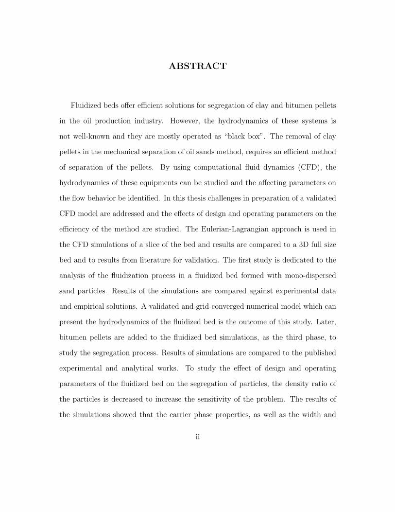
ABSTRACT
Fluidized beds offer efficient solutions for segregation of clay and bitumen pellets
in the oil production industry. However, the hydrodynamics of these systems is
not well-known and they are mostly operated as “black box”. The removal of clay
pellets in the mechanical separation of oil sands method, requires an efficient method
of separation of the pellets. By using computational fluid dynamics (CFD), the
hydrodynamics of these equipments can be studied and the affecting parameters on
the flow behavior be identified. In this thesis challenges in preparation of a validated
CFD model are addressed and the effects of design and operating parameters on the
efficiency of the method are studied. The Eulerian-Lagrangian approach is used in
the CFD simulations of a slice of the bed and results are compared to a 3D full size
bed and to results from literature for validation. The first study is dedicated to the
analysis of the fluidization process in a fluidized bed formed with mono-dispersed
sand particles. Results of the simulations are compared against experimental data
and empirical solutions. A validated and grid-converged numerical model which can
present the hydrodynamics of the fluidized bed is the outcome of this study. Later,
bitumen pellets are added to the fluidized bed simulations, as the third phase, to
study the segregation process. Results of simulations are compared to the published
experimental and analytical works. To study the effect of design and operating
parameters of the fluidized bed on the segregation of particles, the density ratio of
the particles is decreased to increase the sensitivity of the problem. The results of
the simulations showed that the carrier phase properties, as well as the width and
ii

the height of the bed, are not affecting the final degree of the mixture. However, the
rate of segregation of particles is increased by reducing the static height of the bed.
Also, the model showed that there should be an optimum inlet velocity at which
the rate of segregation of particles is fastest and which produces the best level of
segregation of particles, as expected. Among the tested values in the current study
the inlet velocity of 1.25 times the minimum fluidization velocity of the jetsam was
the fastest rate of segregation and most segregated state of the mixture.
iii

To my dear mother, Farah, and my late father, Mehdi.
For all their love, kindness and support.
iv

ACKNOWLEDGEMENT
I would like to acknowledge my supervisor, Dr. Carlos F. Lange, for his kind and
continuous help and understanding.
Also I would like to acknowledge the WestGrid (www.westgrid.ca) and Compute
Canada Calcul Canada (www.computecanada.ca) by which this computationally ex-
tensive research was enabled.
v
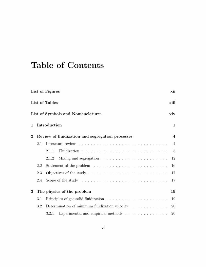
Table of Contents
List of Figures xii
List of Tables xiii
List of Symbols and Nomenclatures xiv
1 Introduction 1
2 Review of fluidization and segregation processes 4
2.1 Literature review . . . . . . . . . . . . . . . . . . . . . . . . . . . . . 4
2.1.1 Fluidization . . . . . . . . . . . . . . . . . . . . . . . . . . . . 5
2.1.2 Mixing and segregation . . . . . . . . . . . . . . . . . . . . . . 12
2.2 Statement of the problem . . . . . . . . . . . . . . . . . . . . . . . . 16
2.3 Objectives of the study . . . . . . . . . . . . . . . . . . . . . . . . . . 17
2.4 Scope of the study . . . . . . . . . . . . . . . . . . . . . . . . . . . . 17
3 The physics of the problem 19
3.1 Principles of gas-solid fluidization . . . . . . . . . . . . . . . . . . . . 19
3.2 Determination of minimum fluidization velocity . . . . . . . . . . . . 20
3.2.1 Experimental and empirical methods . . . . . . . . . . . . . . 20
vi
3.2.2 Theoretical method . . . . . . . . . . . . . . . . . . . . . . . . 21
3.3 Solid particles classification . . . . . . . . . . . . . . . . . . . . . . . 23
3.4 Fluidization regimes . . . . . . . . . . . . . . . . . . . . . . . . . . . 24
3.5 Multiphase modelling approaches . . . . . . . . . . . . . . . . . . . . 28
3.5.1 Carrier phase governing equations . . . . . . . . . . . . . . . . 28
3.5.2 Dispersed phase governing equations . . . . . . . . . . . . . . 30
3.6 Mixing and segregation . . . . . . . . . . . . . . . . . . . . . . . . . . 49
3.6.1 Introduction . . . . . . . . . . . . . . . . . . . . . . . . . . . . 49
3.6.2 Segregation causes and mechanisms . . . . . . . . . . . . . . . 49
3.6.3 Assessing the mixture . . . . . . . . . . . . . . . . . . . . . . 51
4 Numerical method 53
4.1 Solver: cfdemSolverPiso . . . . . . . . . . . . . . . . . . . . . . . . . 56
4.1.1 Governing equations . . . . . . . . . . . . . . . . . . . . . . . 56
4.1.2 Solution algorithm . . . . . . . . . . . . . . . . . . . . . . . . 57
4.1.3 File structure . . . . . . . . . . . . . . . . . . . . . . . . . . . 59
4.2 Model setup . . . . . . . . . . . . . . . . . . . . . . . . . . . . . . . . 60
4.2.1 Geometry . . . . . . . . . . . . . . . . . . . . . . . . . . . . . 60
4.2.2 Mesh . . . . . . . . . . . . . . . . . . . . . . . . . . . . . . . . 60
4.2.3 Boundary conditions . . . . . . . . . . . . . . . . . . . . . . . 60
4.2.4 Materials . . . . . . . . . . . . . . . . . . . . . . . . . . . . . 63
4.2.5 Numerical schemes . . . . . . . . . . . . . . . . . . . . . . . . 63
4.2.6 Initial conditions . . . . . . . . . . . . . . . . . . . . . . . . . 64
4.2.7 Computational method . . . . . . . . . . . . . . . . . . . . . . 64
5 Simulation of fluidization process 67
vii
5.1 Reference simulation run . . . . . . . . . . . . . . . . . . . . . . . . . 68
5.2 Grid sensitivity analysis . . . . . . . . . . . . . . . . . . . . . . . . . 70
5.2.1 2D grid sensitivity analysis . . . . . . . . . . . . . . . . . . . . 70
5.2.2 3D grid sensitivity analysis . . . . . . . . . . . . . . . . . . . . 72
5.3 Effect of the drag coefficient . . . . . . . . . . . . . . . . . . . . . . . 74
5.4 Effect of the boundary conditions . . . . . . . . . . . . . . . . . . . . 80
5.5 Model A and Model B . . . . . . . . . . . . . . . . . . . . . . . . . . 83
6 Simulation of segregation of particles in fluidized bed 86
6.1 Lacey mixing index . . . . . . . . . . . . . . . . . . . . . . . . . . . . 87
6.1.1 Box width . . . . . . . . . . . . . . . . . . . . . . . . . . . . . 87
6.1.2 Sample size . . . . . . . . . . . . . . . . . . . . . . . . . . . . 90
6.2 Validation . . . . . . . . . . . . . . . . . . . . . . . . . . . . . . . . . 91
6.3 Sand and bitumen . . . . . . . . . . . . . . . . . . . . . . . . . . . . 94
6.3.1 Effect of the boundary conditions and momentum exchange
model . . . . . . . . . . . . . . . . . . . . . . . . . . . . . . . 95
6.4 Clay and bitumen . . . . . . . . . . . . . . . . . . . . . . . . . . . . . 108
6.4.1 Aspect ratio of the bed . . . . . . . . . . . . . . . . . . . . . . 109
6.4.2 Carrier phase . . . . . . . . . . . . . . . . . . . . . . . . . . . 110
7 Conclusion and future work 112
7.1 Conclusion . . . . . . . . . . . . . . . . . . . . . . . . . . . . . . . . . 112
7.2 Future work . . . . . . . . . . . . . . . . . . . . . . . . . . . . . . . . 114
A Dictionary files 126
B Mixing index code 132
viii

List of Figures
3.1 Pressure drop in a bed versus fluid velocity. Adapted from [Kunii and
Levenspiel, 1969] . . . . . . . . . . . . . . . . . . . . . . . . . . . . . 21
3.2 Geldart powder classification. Adapted from [Geldart, 1973]. . . . . . 24
3.3 Fluidization regimes map. Adapted from [Kunii and Levenspiel, 1997] 27
3.4 Displacement of two particles in contact. Adapted from [Crowe et al.,
2011] . . . . . . . . . . . . . . . . . . . . . . . . . . . . . . . . . . . . 44
3.5 Contact forces in particle collision. Adapted from [Crowe et al., 2011] 46
3.6 Mixtures types. Adapted from [Rhodes, 2008]. . . . . . . . . . . . . . 49
4.1 CFDEM ® coupling file structure. . . . . . . . . . . . . . . . . . . . . 61
4.2 Schematic of the geometry, mesh, and initial conditions of the model.
(a) Preparation of the initial condition of the bed by inserting particles
at random positions in domain. (b) Initial condition of fluidization
process. (c) Initial condition of the segregation process - mixed. (d)
Initial condition of the segregation process - segregated. (e) Side view
of the bed. . . . . . . . . . . . . . . . . . . . . . . . . . . . . . . . . 62
5.1 ANSV of 2D grid sensitivity analysis . . . . . . . . . . . . . . . . . . 71
ix
5.2 Pressure drop and ANSV versus number of nodes - 2D refinement of
a slice of the bed. . . . . . . . . . . . . . . . . . . . . . . . . . . . . . 72
5.3 ANSV of 3D grid sensitivity analysis . . . . . . . . . . . . . . . . . . 73
5.4 Pressure drop and ANSV versus number of nodes - 3D refinement of
a slice of the bed. . . . . . . . . . . . . . . . . . . . . . . . . . . . . . 74
5.5 Bed pressure drop versus NRT of three different drag models . . . . . 76
5.6 Pressure drop in a poorly fluidized beds. Adapted from [Kunii and
Levenspiel, 1969] . . . . . . . . . . . . . . . . . . . . . . . . . . . . . 76
5.7 Contour of sand volume fraction of bed using Koch & Hill drag model 77
5.8 ANSV versus NRT for three different drag models. . . . . . . . . . . 78
5.9 Comparison of time averaged void fraction of the bed for three different
drag models at z=0.02 m (a) and z=0.05 m (b). . . . . . . . . . . . . 79
5.10 Comparison of time averaged particles velocity using three different
drag models. . . . . . . . . . . . . . . . . . . . . . . . . . . . . . . . . 79
5.11 Time averaged particle-fluid momentum exchange of the bed of three
different drag models. . . . . . . . . . . . . . . . . . . . . . . . . . . . 80
5.12 Bed pressure drop versus NRT for frictional wall and periodic bound-
ary conditions. . . . . . . . . . . . . . . . . . . . . . . . . . . . . . . 81
5.13 ANSV versus NRT for frictional wall and periodic boundary conditions. 82
5.14 Time averaged void fraction of the bed of frictional wall and periodic
boundary conditions at z = 0.02 m (a) and z=0.05 m (b). . . . . . . . 83
5.15 Bed pressure drop using Model A and Model B for momentum ex-
change term. . . . . . . . . . . . . . . . . . . . . . . . . . . . . . . . . 85
5.16 ANSV versus NRT, Model A and Model B for momentum exchange
term. . . . . . . . . . . . . . . . . . . . . . . . . . . . . . . . . . . . . 85
x
6.1 Particles’ mean height in time. . . . . . . . . . . . . . . . . . . . . . . 89
6.2 Standard deviation of particles’ height in time. . . . . . . . . . . . . . 89
6.3 Effect of sample size on the Lacey mixing index in time. . . . . . . . 90
6.4 Comparison of pressure drop in bed using Model A when superficial
gas velocity is 1.2 m s−1. . . . . . . . . . . . . . . . . . . . . . . . . . 92
6.5 Comparison of pressure drop in bed using Model B when superficial
gas velocity is 1.2 m s−1. . . . . . . . . . . . . . . . . . . . . . . . . . 93
6.6 Comparison of Lacey mixing index from simulations with results from
Feng and Yu [2004]. . . . . . . . . . . . . . . . . . . . . . . . . . . . . 94
6.7 Effect of discrete phase boundary condition on Lacey mixing index -
Model A. . . . . . . . . . . . . . . . . . . . . . . . . . . . . . . . . . . 97
6.8 Effect of discrete phase boundary condition on Lacey mixing index -
Model B. . . . . . . . . . . . . . . . . . . . . . . . . . . . . . . . . . . 97
6.9 Comparison of effect of boundary conditions on ANSV versus NRT
for sand and bitumen using Model A and B. . . . . . . . . . . . . . . 99
6.10 Effect of initial condition on Lacey mixing index - Periodic boundary
condition. . . . . . . . . . . . . . . . . . . . . . . . . . . . . . . . . . 101
6.11 Snapshot of the bed at different times - periodic boundary conditions
and Model A. . . . . . . . . . . . . . . . . . . . . . . . . . . . . . . . 102
6.12 Snapshot of the bed at different times - periodic boundary conditions
and Model B. . . . . . . . . . . . . . . . . . . . . . . . . . . . . . . . 102
6.13 Effect of initial condition on Lacey mixing index - frictional wall
boundary condition. . . . . . . . . . . . . . . . . . . . . . . . . . . . 103
6.14 Snapshot of the bed at different times - frictional wall boundary con-
ditions and Model A. . . . . . . . . . . . . . . . . . . . . . . . . . . . 104
xi
6.15 Snapshot of the bed at different times - frictional wall boundary con-
ditions and Model B. . . . . . . . . . . . . . . . . . . . . . . . . . . . 105
6.16 Effect of superficial inlet velocity on Lacey mixing index (a) Model A
and (b) Model B. . . . . . . . . . . . . . . . . . . . . . . . . . . . . . 107
6.17 Effect of bed aspect ratio on Lacey mixing index. . . . . . . . . . . . 110
6.18 Effect of carrier phase properties on Lacey mixing index. . . . . . . . 111
xii

List of Tables
3.1 Mixing indices. Adapted from [Poux et al., 1991]. . . . . . . . . . . . 51
4.1 Governing equations used in Eulerian - Lagrangian approach for sim-
ulation of fluidization process and segregation process . . . . . . . . . 57
4.2 Parallel efficiency test results on Jasper server. . . . . . . . . . . . . . 65
5.1 Reference simulation run setup . . . . . . . . . . . . . . . . . . . . . 68
5.2 2D grid sensitivity analysis, grid size and statistical information . . . 70
5.3 3D grid sensitivity analysis, grid size and statistical information. . . . 73
5.4 Momentum exchange term models and forces . . . . . . . . . . . . . . 84
6.1 Sample size . . . . . . . . . . . . . . . . . . . . . . . . . . . . . . . . 88
6.2 Parameters used for the validation case adapted from Feng and Yu
[2004] . . . . . . . . . . . . . . . . . . . . . . . . . . . . . . . . . . . 91
6.3 Reference simulation settings . . . . . . . . . . . . . . . . . . . . . . . 95
6.4 Different boundary conditions used in simulation models. . . . . . . . 96
6.5 Superficial inlet velocities. . . . . . . . . . . . . . . . . . . . . . . . . 106
6.6 Bed dimensions. . . . . . . . . . . . . . . . . . . . . . . . . . . . . . . 109
6.7 Carrier phase properties. . . . . . . . . . . . . . . . . . . . . . . . . . 110
xiii
List of Symbols and
Nomenclatures
Greek
β Fluid-particle friction coefficient (kg m−3 s−1)
δn Displacement of the particle in normal direction (m)
δt Displacement of the particle in tangential direction (m)
εg Gas void fraction (-)
εg,mf Gas void fraction at minimum fluidization condition (-)
εs Particles void fraction (-)
ηnj Damping coefficient of the particle in normal direction (-)
ηtj Damping coefficient of the particle in tangential direction (-)
Θ Granular temperature (m2 s−2)
γ Dissipation due to inelastic collisions (-)
ν Poisson ratio (-)
xiv
ω Particle angular velocity (s−1)
φs Sphericity of the particle (-)
ρg Gas density (kg m−3)
ρp,i Density of particle i (kg m−3)
ρs Solid density (kg m−3)
τ Reynolds shear stress (kg m−1 s−2)
µg Gas viscosity (kg m−1 s−1)
ξ A constant for drag factor (-)
Roman
A Cross-sectional area of the bed (m2)
Ap Particle projection area (m2)
CD Drag coefficient (-)
C Particles’ velocity fluctuations (m s−2)
d Diameter of the particle (m)
dp Mean diameter of the particles (m)
d∗ Dimensionless measure of particle diameter (-)
f Drag factor (-)
xv

e Coefficient of restitution (-)
F A constant for drag factor (-)
F0 A constant for drag factor (-)
F3 A constant for drag factor (-)
fdrag,i Drag force on particle i (kg m s−2)
fp−f,i The force imposed by the carrier phase to particle i (kg m s−2)
Fnij Normal force between particles i and j (kg m s−2)
Ftij Tangential force between particles i and j (kg m s−2)
fc,ij Contact force between particles i and j
fd,ij Damping force between particles i and j
FA Volumetric particle-fluid interaction force, model A (kg m s−2)
FB Volumetric particle-fluid interaction force, model B (kg m s−2)
g Gravity acceleration (m s−2)
G Relative velocity of particle at contact point (m s−1)
Gct Slip velocity of particle at contact point (m s−1)
G Shear modulus (kg m−1 s−2)
H Static height of the bed (m)
Ii Rotational inertial momentum of particle i (kg m2)
xvi
k Permeability (m2)
kn Stiffness in normal direction (-)
kt Stiffness in tangential direction (-)
L Length of the bed (m)
mi Mass of the particle i (kg)
n Normal vector
kc Total number of particles in a computational cell (-)
n Number of particles (-)
P Overall portion of a component of the mixture (-)
∆po Hydrostatic pressure drop (kg m−1 s−2)
∆pd Hydrodynamic pressure drop (kg m−1 s−2)
∆p Total pressure drop (kg m−1 s−2)
Ps Solid pressure (kg m−1 s−2)
∆pw Frictional pressure drop (kg m−1 s−2)
r Particle radius (m)
Re Reynolds Number
Tg Gas phase stress tensor (kg m−1 s−2)
Ts Solid phase stress tensor (kg m−1 s−2)
xvii
Umf Superficial inlet velocity of the gas at minimum fluidization condition (m s−1)
Umf,jetsam Minimum fluidization velocity of the jetsam (m s−1)
v Particle velocity (m s−1)
u∗ Dimensionless gas velocity (-)
U Superficial inlet velocity of the gas (m s−1)
Vp,i Volume of the particle i (m3)
∇V Volume of the computational cell (m3)
W Total weight of the particles (kg m s−1)
Y Young modulus (kg m−1 s−2)
xviii

Chapter 1
Introduction
Canada has the world’s third-largest proved reserves of crude oil, ninety percent
of which, or 169 billion barrels, are found in the tar sands. Considering the daily
production rate of oil from the Alberta’s tar sands, 2.3 million bpd in 2014 [Alberta,
2016], it is imperative to develop new methods of oil extraction to reduce the cost of
the production and the footprint on the landscape [Honarvar et al., 2011].
Current methods of extraction of oil from tar sands, surface mining, steam as-
sisted gravity drainage (SAGD), cyclic steam stimulation (CSS) or vapor extraction
(VAPEX), require tremendous amounts of water, up to ten times the produced oil,
energy and sometimes solvents. The Energy Returned On Energy Invested “EROEI”
of these methods is about 5 to 6 [Board, 2006], which increases the total production
cost and has serious effects on the environment. Also, residual hydrocarbons along
with the clay are disposed of in oil sand tailing ponds, which are another concern
of environmentalists. A new approach with a higher EROEI, which consumes fewer
resources, while producing less pollution, is required to turn oil sands business into
an efficient and green business.
1

A novel method was proposed and patented by Duma [2012] for mechanical pro-
cessing of tar sands. In this process pellets of tar sands are formed by grinding
oil sands and cooling down below the transition temperature, -25 °F, so that they
do not aggregate and remain as distinct units. Because of impurities in the ore, a
fraction of the pellets will unavoidably contain only clay, instead of oil sands. After
pelletization, the clay pellets are separated from the oil sand pellets by means of a
fluidized bed. Later, pellets are fractured using mechanical methods, e.g. by a ball
mill or a hammer mill, to separate the bitumen from the sand.
A key point in this process is an efficient method of separation of clay and bitumen
pellets in the fluidized bed. This will remove clay in the early stages of the process.
This thesis aims to examine the process of separation of oil sand pellets from clay
pellets in the fluidized bed of the mechanical processing of tar sands method.
It was early 1930’s that the fluidization process and fluidized beds were intro-
duced to the industry and they were developed more after World War II when a
group of companies, Standard Oil New Jersey, M.W. Kellogg, Shell and Universal
Oil Products designed the catalytic cracking method for gasoline [Yates, 2013]. “Fine
solid particles are transformed into a fluid-like state, when they are in contact with
a flow of gas, and they possess the behavior of a fluid” [Kunii and Levenspiel, 1997].
Researchers have performed numerous investigations on the operating parameters
of a fluidized bed, such as the inlet velocity, density of particles, mass flux, and their
mutual interactions, due to the extensive applications of fluidized-beds nowadays in
industry [Cheremisinoff and Cheremisinoff, 1984].
The scale-up of the pilot-scale device to the full size and commercial device de-
pends on many factors, which will be discussed in the following chapters. Even with
the most conservative approaches, final designs do not always fulfill the expecta-
tions. This is because, although the hydrodynamics of these systems have been well
2

studied, unified equations and models to describe the bubble formation and particle
interactions have not yet been developed. Without a real knowledge of the fluidiza-
tion process, it is not possible to design an optimized fluidized bed. This requires the
investigation of the fluidization process in depth by considering fundamentals of mass
transfer, momentum transfer, heat transfer and chemical reaction [Cheremisinoff and
Cheremisinoff, 1984].
With the improved computational power and algorithms, it is possible to model
fluidized beds in pilot size and also industrial size as well [Stanek, 1994].
The literature review, to be discussed in next chapter, revealed that factors, such
as carrier phase properties, particles size ratio and density ratio, and operating con-
ditions of the bed are significant factors of the fluidization and separation processes.
The objective of this thesis is to employ computational fluid dynamics (CFD)
techniques to produce a validated and grid-converged numerical model for fluidization
and segregation processes and analyze the effect of bed operating parameters on the
quality of the mixture. A literature review on experimental and numerical works
on gas-solid fluidization and utilization of fluidized beds is presented in Chapter
2. Principles of gas-solid fluidized beds, classification of particles and fluidization
regimes, physical approaches and governing equations of the fluidized beds, principles
of mixing and segregation of particles and available methods of assessing the quality
of mixtures are discussed in Chapter 3. Numerical algorithms and the software,
materials, model setup and the methodology are discussed in details in Chapter
4. Results of the simulation of fluidization process and analysis of the results are
presented in Chapter 5. Chapter 6 is dedicated to the simulation of the segregation
process, and results of simulations are discussed and analyzed. Finally, conclusions
and recommendations are given in Chapter 7.
3
Chapter 2
Review of fluidization and
segregation processes
2.1 Literature review
The first large-scale, industrial fluidized bed was designed for coal gasification by
Fritz Winkler and patented in 1922 (D.R.P. 437,970). Fluidized beds are widely
used in industrial applications due to their unique and unusual but useful, behavior.
The advantages of fluidized beds can be summarized as below [Kunii and Levenspiel,
1997]:
• Ease of operating control in continuous processes due to the smooth and fluid
like flow of particles.
• Rapid preparation of a homogeneous mixture or of a segregated mixture of
particles due to their density or size ratio.
• High rates of gas - solid mass and heat transfer, compared to other contacting
4
methods.
Mixing of fine powders, segregation of particles, heat exchange and gasification of
powders, drying, coating, agglomeration and sizing of particles, and many other
processes can be named as industrial applications of fluidized beds which benefit from
the advantages of the fluidization process. However, their complex hydrodynamics
can lead to the faulty design of a fluidization process. Formation of big bubbles or
slug flows are some of the issues that can affect the performance of the fluidized bed.
[Kunii and Levenspiel, 1997]
The high rate of heat transfer and sensitivity of mixture to density and size ratio
in fluidized beds can have significant desirable effects on the separation of bitumen
pellets from clay in mechanical processing of oil sands.
2.1.1 Fluidization
Fluidization refers to transforming fine solid particles, that are initially at rest in a
cylinder, to a fluid state using an upward flow [Kunii and Levenspiel, 1997]. The
hydrodynamics of fluidized beds at minimum fluidization conditions and equations of
minimum fluidization velocity and pressure drop in bed were studied and developed
by Ergun [1952]. The physics and regimes of the fluidized beds are described in
Chapter 3.
Geldart [1973] and Geldart and Abrahamsen [1978] classified particles into four
major groups (A, B, C and D) based on their behavior, when they are suspended
in gas, to study the fluidization process. Kunii and Levenspiel [1997] classified flu-
idization regimes in fluidized beds into packed bed, bubbling fluidized bed or spouted
fluidized bed, and circulating fluidized bed regimes which contain turbulent fluidized,
fast fluidized, and pneumatic transport sub-regimes. These experimental classifica-
5
tions will help identify the flow regime applicable to the present study, which is
essential to the selection of the numerical approach, as will be described next.
There are two main approaches to multiphase flow analysis and simulation of
fluidization process, namely the Eulerian - Eulerian approach, which is also known
as two-fluid model (TFM), and the Eulerian - Lagrangian approach, also known as
discrete element method (CFD-DEM). The Eulerian - Eulerian approach was used
to analyze the hydrodynamics of large-scale fluidized bed by many researchers. In
this method [Crowe et al., 2011], the solid phase is treated as a continuous phase
with equivalent properties of a fluid. Empirical and semi-empirical models have been
developed to describe the equivalent dispersed phase properties. In the constant vis-
cosity model, the solid phase viscosity is assumed to be a constant and the solid phase
pressure is considered to be only a function of the local solid porosity and viscosity.
The kinetic theory of dense gasses later was developed to model the properties of
the solid phase in the Eulerian approach. Equations of granular temperature, solid
pressure and viscosity, and particles drag model in particles cloud were developed
and reviewed by Gidaspow [2012]. The hydrodynamics of fluidized beds have been
widely studied and analyzed using the Eulerian - Eulerian approach in computational
fluid dynamics method by many researchers [Gidaspow, 2012].
Van der Hoef et al. [2006] reviewed the developments on multiscale modeling of
gas-solid fluidized beds at that time. This report covered Eulerian - Eulerian and
Eulerian - Lagrangian approaches. The result of TFM simulations might be grid
independent, if the size of the grid is on the order of few particle diameters (≈ 10).
As the Eulerian approach requires a fine grid to produce accurate results, time steps
of the order of 10−5 s should be used in a simulation, which is not feasible for
simulation of commercial size fluidized bed. To overcome this problem, commercial
scale fluidized beds are simulated over coarse spatial grids. In these coarse grids,
6
small-scale spatial structures are not resolved. The effect of these small-scale spatial
structures are added to the system by modification of the closure equations. A proper
method of modification of the closure problems is still an open topic in research
[Van der Hoef et al., 2006].
A review of the developments of multiscale CFD of modeling gas-solid circulating
fluidized bed (CFB) modeling byWang et al. [2010] shows that, although the Eulerian
- Eulerian approach might reach grid independent solution with conventional drag
models in periodic domains, the drag force is overestimated and it fails to predict
the S-shape of the axial voidage profile [Wang et al., 2010].
Mortier et al. [2011] reviewed the research works on granules drying application of
fluidized beds. The authors reviewed both TFM and Lagrangian approaches in CFD
modeling of fluidized beds. Using the TFM approach, physical characteristics of the
dispersed phase, such as size and shape, are included through empirical relations and
particles are not modeled as distinct particles. Comparing results of numerical studies
and experimental works, the Lagrangian approach results are in better agreement
with experimental data [Chiesa et al., 2005, Mortier et al., 2011].
Singh et al. [2013] reviewed the CFD modeling of combustion and gasification
of fuels in fluidized beds. Simulation of gasification and combustion in commercial
fluidized beds is still an open topic of research. The TFM approach is not suitable
for simulation of fluidized bed with particle size variation unless extensive approxi-
mations are chosen. In addition in thermo-chemical reactions there is no appropriate
model to describe the mechanism of reactions in commercial fluidized beds using
the Eulerian approach. The Eulerian - Lagrangian approach seems to predict better
results in thermo-chemical reactions. However, this approach is computationally ex-
pensive compared to TFM method, which makes it not to be suitable for commercial
size fluidized beds [Singh et al., 2013].
7

Azimi [2014] reviewed the research works on coal separation in Air Dense Medium
Fluidized Beds (ADMFB). Comparing results of simulations and experimental work
for separation of coal and sand, poor results were achieved in most preliminary 2D
simulations due to the inaccuracy and incapability of Eulerian - Eulerian approach
in predicting interactions in the transient regime, at the stage of developing bubbles.
However, the predictability of the model was significantly improved by modification
of the drag model, coefficient of restitution and using a 3D domain in the simulation
[Azimi, 2014].
Zhong et al. [2016] published a comprehensive review of the developments in the
CFD simulation of fluidized beds and dense particulate systems using Eulerian -
Eulerian approach. Particle size changes, shrinkage or agglomeration, are not ad-
dressed adequately in Eulerian - Eulerian approach, and sub-models are required to
be developed in this approach [Zhong et al., 2016].
A review of the significant applications and advances in discrete particle simula-
tion of particulate systems was done by Zhu et al. [2008]. The report covers particle
packing, particle flow, and particle-fluid flows. The theoretical developments in dis-
crete particle simulation of particular systems are addressed in another article by
Zhu et al. [2007]. This review covers research works and developments on modeling
particle-particle and particle-fluid interactions and coupling discrete element method
with CFD in particle-fluid flows. The simulation of local average method of the gas
phase coupled with the discrete element method (DEM) simulation of the solid phase
can describe the characteristics of particle-fluid flows without any general assump-
tion. This method produces results which can be used for a better understanding of
granular materials and particulate systems and it could be used to study the micro-
properties of granular materials to test continuum approaches in granular materials
[Zhu et al., 2007].
8
The performance of particulate systems and multiphase processes mostly falls
under 60% of the designed capacity, despite their wide industrial application [Zhu
et al., 2008]. Many of multiphase processes are operated as “black box” reactors.
This is mainly due to the complex dynamics of particles interactions. The bulk
behavior of a reactor depends on the collective outcome of particles interactions.
The DEM approach can reveal the underlying fundamentals of particulate system,
that make it suitable for detailed studies of such systems [Zhu et al., 2008].
The DEM approach was first proposed by Cundall and Strack [1979] for geome-
chanics research to describe the behavior of assemblies of discs and spheres. The
DEM was later coupled to the CFD to model a two-dimensional fluidized bed by
Tsuji et al. [1993]. In this method, the discrete phase is modeled by using the DEM
approach, that is based on Newton’s laws of motion, and the carrier phase is modeled
by the locally averaged variables method, first introduced by Anderson and Jackson
[1967]. Due to the high demand of computational power by the DEM approach,
progress in this area has been slow in the past. With the currently available compu-
tational power, the coupled CFD and DEM has been used in many pieces of research
to describe the particle-fluid flow [Zhu et al., 2008].
Zhou et al. [2010] assessed and verified available formulations of momentum equa-
tion sets for the particle phase and fluid phase, namely set I, set II and set III, which
will be reviewed in Chapter 3. Comparing results of simulations for different par-
ticulate systems, they recommended set II, and set I for future work in CFD-DEM
simulation of particulate systems. However, the third set of equations conditionally
can be used when the fluid flow is steady and uniform or the residual force acting on
particles is zero [Zhou et al., 2010].
Xu and Yu [1997] studied the hydrodynamics of fluidized bed by using a coupled
CFD and DEM approach. Plots of bed pressure drop versus superficial inlet velocity
9

were created for both increasing and decreasing inlet velocity cases. Results are in
good agreement with measured pressure drop values from experimental works and
the same trends were observed.
Goldschmidt et al. [2004] compared simulation results from DEM using a hard
sphere approach simulation results and TFM simulation results with experimental
results of a fluidized bed. They showed that the DEM approach results were in
better agreement with experimental results compared to TFM approach. Complex
structures such as formation of small bubbles near the bottom of the bed and strings
of particles within larger bubbles were captured using the DEM approach. Compar-
ing results of both CFD models, the kinetic theory of granular flow was capable of
giving a meaningful estimate of particles’ fluctuating velocities. However, regarding
bed expansion dynamics, their simulations results did not follow their experiments.
The deviation is mainly due to the formation of densely packed regions in which
particles movements approach zero. CFD models were not able to capture these re-
gions. Using the hard sphere discrete particle method, it is not possible to model the
long-term particle contacts and multi-particle interactions. Also in TFM approach,
when kinetic theory of granular flows is used for closure problems, these contacts are
neglected [Goldschmidt et al., 2004].
Muller et al. [2009] validated results of DEM simulations of a fluidized bed against
experimental data extracted by magnetic resonance measurements technique. They
showed that simulation results are insensitive to the value of restitution coefficient
and coefficient of friction, as long as particle-particle and particle-wall collisions
energies are dissipated by some routes in the simulations [Muller et al., 2009].
Goniva et al. [2012] studied the influence of rolling friction on a single spout flu-
idized bed. An open source code was developed based on their work, CFDEM®coupling
[Goniva et al., 2012], which couples the CFD solver, OpenFOAM [Weller et al., 1998],
10
with DEM solver, LIGGGHTS [Kloss et al., 2012] (based on LAMMPS [Plimpton,
1995]). By applying a rolling frictional model, the angle of the response of a granular
material can be predicted more accurately. In a 2D spouted fluidized bed, the rolling
friction can play a significant role in the results of simulations, especially in regions
close to the side walls. The wall effect increases by increasing the rolling coefficient.
The particle velocity is affected by the wall at the regions close to wall [Goniva et al.,
2012].
Deb and Tafti [2012] used DEM coupled with their in-house developed CFD code,
GenIDLEST, to simulate a 2D fluidized bed with a single jet at the inlet. Later, they
extended the work to model the fluidized bed with multiple jets at the inlet. Results
of numerical simulations are in good agreement with their experimental work in the
region close to the distributor plate. However, the code was not able to capture three-
dimensional structures at the free surface of the bed which resulted in deviation of
simulation results and experimental work results [Deb and Tafti, 2012].
He et al. [2009] studied the hydrodynamics of fluidized beds by comparing results
of DEM simulations of a 3D fluidized bed with experiments using PIV technique.
They showed that the superficial inlet velocity had a significant effect on the verti-
cal solid velocity and the extent of solids downflow. Also comparing results of the
mean time averaged vertical solid velocity, they confirmed, that for averaging pe-
riods longer than 12.5 s, the results of the mean and RMS velocity changes with
changing/increasing the averaging period slightly [He et al., 2009].
Traore et al. [2014] simulated 2.7 millions of particles for 1 s on a cluster with 246
Opteron processors. Evolution of a single bubble from its formation until its explosion
at the bed surface, the formation of “worm-like-shaped” structures as displayed by
Tsuji et al. [2008], and occurrence of the bubbly regime were simulated using an
efficient 4-way coupling CFD-DEM approach [Traore et al., 2014].
11
2.1.2 Mixing and segregation
In bubbling fluidized bed, if solid particles with different physical properties, such
as density, diameter, shape, are simultaneously fluidized, their different fluidization
behavior leads to inhomogeneity of solid composition along the bed height. Particles
which are accumulated at the bottom of the bed are referred to jetsam, while the
other component, that occupies the top portion of the bed, is referred to flotsam
[Rowe et al., 1972].
Mixing and segregation of particles have been studied by many researchers in
experiments [Palappan and Sai, 2008a,b, Rao et al., 2011], analytical approaches
[Daw and Frazier, 1988, Di Maio et al., 2013, Gibilaro and Rowe, 1974], and numer-
ical studies [Di Renzo et al., 2008, Huilin et al., 2007]. Gibilaro and Rowe [1974]
used simplified partial differential equations to model analytically a segregating gas
fluidized bed. Based on their proposed models, four physical mechanisms exist in
segregation of particles in a fluidized bed, namely overall particle circulation, an in-
terchange between wake and bulk phases, axial spreading and a relative segregating
flow rate. The model was successful in predicting the equilibrium segregation pro-
files in a gas fluidized bed for three segregation patterns, namely strongly segregating
systems, perfect mixing, and intermediate case [Gibilaro and Rowe, 1974].
On another attempt Daw and Frazier [1988] studied the segregation of large
particles (d ∼ 3 mm) in gas fluidized bed and correlated the mixing index, which
will be explained in Section 3.6.3, to particles size ratio, density ratio, static height
of the bed, and the superficial inlet velocity. However, correlations for small particles
and different geometries of fluidized beds were not covered in their report [Daw and
Frazier, 1988].
Rao et al. [2011] reviewed the investigations on segregation of a binary mixture of
12
particles comprehensively. A new classification scheme for the minimum fluidization
velocity ratio, pressure drop profiles, and segregation behavior of binary fluidized
mixtures was proposed by comparison of published data and experiments. This
classification is based on particles size and density ratio and consists of seven mixture
types [Rao et al., 2011].
The experimental values and models, as described before, can be applied to val-
idate the numerical works. CFD has been used by many researchers to study hy-
drodynamics of mixing and segregation of particles in fluidized beds numerically
[Bokkers et al., 2004, Di Renzo et al., 2008, 2012, Feng and Yu, 2004, 2007, 2009,
Huilin et al., 2007, Luo et al., 2015, Moon et al., 2007, Rhodes et al., 2001, Wang
et al., 2015].
In 2004, Feng and Yu [2004] used a DEM approach to model segregation and
mixing of particles in a fluidized bed. Two models are introduced in the literature
for momentum conservation equations by using the available models for treatment
of the pressure drop term, coupling schemes, and particle-fluid interaction forces,
namely Model A and Model B. Due to the differences in the formulation of these two
models, the accuracy of each model is still an open topic. A significant difference
was observed between Model A and Model B in comparison of simulation results
with experiment results. Verification of results against experiments, comparison of
pressure drop and concentration of mixture components in height, showed that the
Model B is favorable in the formulation of CFD-DEM modeling of fluidized bed
[Feng and Yu, 2004]. In another study by Feng et al. [2004], they showed that the
stable state of mixing and segregation of particles is strongly affected by the gas
velocity. Later, Feng and Yu [2007] showed that the maximum degree of segregation
of particles can be achieved at a specified gas velocity for a binary mixture of particles.
They suggested that both particle-particle and particle-fluid forces play a significant
13
role in the separation and mixing of particles. These forces vary both spatially and
temporally, which makes their behavior complicated. In another work, Feng and Yu
[2009] showed that in a bi-sized mixture of particles the density ratio of the jetsam
and flotsam is the dominant parameter that controls the degree of mixing of particles.
Bokkers et al. [2004] studied the mixing of particles of same size and density in a
fluidized bed, which are marked by color difference only. They examined the effect
of drag model on the formation of bubbles and degree of mixing and compared the
results with experimental results. They showed that the Koch and Hill [Hill et al.,
2001a] drag model predicted better results than the Ergun [Ergun, 1952] equation
combined with Wen and Yu closures [Wen and Yu, 2013]. Besides, they showed that
soft sphere and hard sphere models predict the same bubble size and shape.
Luo et al. [2015] studied mixing of particles of same size and density in a fluidized
bed using the DEM approach. The CFD-DEM approach was successful in predicting
the solid circulation pattern and formation of bubbles. The superficial inlet gas
velocity has affects the bubble size that controls the rate of solid mixing.
Moon et al. [2007] used an equation-free coarse-grained approach to accelerate the
simulation of segregation process. The method was able to speed up the simulation
by a factor of two to ten. This method can be used to describe the stable state of
the bed.
Di Renzo et al. [2012] compared results of experiments with CFD-DEM simula-
tions of segregation of particles in a fluidized bed and proposed a model to predict
the flotsam component in a binary mixture at equilibrium state. However, the model
is not capable of describing the mixing degree at the macroscopically stable state of
the bed.
Wang et al. [2015] implemented a hybrid TFM-DEM approach to analyze the
segregation of particles in a fluidized bed. The dense solid phase and continuous
14

carrier phase were modeled by TFM approach, while the dilute solid phase was sim-
ulated by DEM approach. Results of simulation were validated against experiments.
They showed that the model is capable of producing similar results as those of ex-
periments. The particle size strongly affects the quality of mixture and segregation
of particles. Particles’ mean height was used to analyze the kinetics of segregation
process. The drag force from the gas phase and continuum solid phase influences the
particles behavior. The segregation of particles is controlled by the summation of
upward drag forces, which is larger than the gravity force on flotsam particles [Wang
et al., 2015].
Rhodes et al. [2001] studied numerically the mixing of particles of same size and
density in a fluidized bed. They used the Lacey mixing index to quantify the quality
of the mixture. The Lacey mixing index was developed based on statistical analysis
of the mixture and it compares the quality of the achieved mixture with the quality of
a completely random mixture. Standard deviation of the volume fraction of mixture
components at different locations of the bed is used in this comparison. Samples at
different locations of the bed are required to estimate the standard deviation of the
volume fraction of mixture components. The DEM approach enables sampling of the
bed without disturbing the mixture. Also, it is possible to change the sample size at
each time step. In experimental works, sampling methods suffer from a transition of
fluidized bed state to fixed bed state. This transition can be avoided in the DEM
approach. They used rectangular boxes to obtain samples. The widths of these boxes
were fixed, and their heights were set according to the number of particles in each
sample box. This method helps to set the level of scrutiny in the estimation of the
mixing index [Rhodes et al., 2001].
15
2.2 Statement of the problem
Considering the increasing demand for low-cost energy and environmental issues
with current oil extraction methods, an economic and green method of oil extraction
should be developed. The mechanical process of tar sands, as described in Chapter
1, may overcome environmental and economic issues related to current processes
of oil extraction. The separation of bitumen and clay in the fluidized bed is a
key point for an efficient method. Although there have been extensive studies on
fluidized beds, valuable information about the hydrodynamics of separation and effect
of operating parameters on the quality of the mixture is not available. It is vital to
analyze the impact of significant factors on the process to design the fluidized bed
at optimum condition. With the available computational power nowadays, it is
possible to simulate the process using the DEM approach. The DEM approach can
increase the accuracy of the results. As it was mentioned in the literature survey,
many researchers up to now have studied the feasibility of implementation of DEM
approach in CFD modeling of fluidized beds. However, the effect of parameters
on the accuracy of results have not been addressed, and there is no general rule
to model the fluidized bed using the DEM approach. It is necessary to study the
effect of parameters on the simulation results to create an accurate numerical model.
Later, the numerical model will be used to examine the effect of design parameters
and operating parameters of the bed on mixing and segregation of particles in the
fluidized bed.
16
2.3 Objectives of the study
Following the discussion of the need for producing a numerical model for fluidized
beds, the objective of this research work is to analyze the effect of significant factors
of a numerical model, such as grid size, boundary conditions, drag coefficient model
and momentum exchange models on simulation results. Then, the numerical model
will be used to study the segregation process in a fluidized bed, and analyze the
effect of design and operating parameters of a fluidized bed, such as superficial inlet
velocity, particles’ density ratio, the physical properties of the carrier phase and the
bed size, on the fluidization and segregation process.
2.4 Scope of the study
One of the significant factors in numerical methods is the size of the grid. The
accuracy of the simulation results using different size of grids is investigated to find
the optimum grid size on which results of simulations are independent of the grid
size. The grid size analysis is based on the fluidization process and the pressure drop
in the bed, as a characteristic quantity, is estimated for this purpose.
In gas-solid fluidized beds, the drag force is a dominant factor. The application
of different drag models could introduce errors on bed expansion, pressure drop and
particles concentration. In the current work, available drag models are examined
and evaluated to obtain an accurate numerical model.
As it was discussed in the literature review, the DEM is a computationally ex-
pensive method. In most of the simulations a slice of the bed is considered as the
simulation domain to reduce the required computational power and time. This as-
sumption affects the results of simulations. The effect of a sliced domain is studied
17
and verified so that a true representation of the 3D fluidized bed is achieved.
The momentum exchange term in the simulation of gas-solid flow is the key
point in the coupling of phases. The effect of the momentum exchange term on the
hydrodynamics of fluidization process is considered using available models, Model A
and Model B [Gidaspow, 2012]. The effect of models on the hydrodynamics of the
fluidization process is examined by comparing the calculated pressure drop with the
value of analytical and empirical solutions.
Further investigations are performed on the segregation of a binary mixture of
spherical particles. At the first step a binary mixture of sand and bitumen at -50℃
with a density ratio of 2.5 is fluidized to be segregated. The effect of front and
back planes is studied, and results are compared with a 3D case. The momentum
exchange model is investigated, and results are compared with literature.
The results of the fluidization process and segregation of particles with density
ratio of 2.5 are used to produce a numerical model for segregation of particles with
a smaller density ratio. The numerical model is used to examine the effect of the
carrier phase and the bed aspect ratio on the rate of segregation and the stable state
of this mixture.
18

Chapter 3
The physics of the problem
3.1 Principles of gas-solid fluidization
Fluidization refers to transforming fine solid particles, that are initially at rest in
a cylinder, to a fluid state using an upward flow. The total pressure loss of the
fluid throughout the bed increases by increasing the superficial inlet velocity from
zero. The pressure drop increases because frictional resistance increases. By further
increase of the gas velocity, particles start to vibrate. At this stage, the weight of
particles is counterbalanced by the frictional force between particles and the fluid
and the pressure drop in the flow field at each height is equal to the overhead weight
of fluid and particles. This state is called minimum fluidization state where particles
are lifted in the flow and are supported by the flow field [Kunii and Levenspiel, 1969].
The dense-phase of particles, when it is fluidized by gas, looks like a boiling liquid.
This fluidized dense phase has some unusual but useful properties of the system.
Some of the behaviors of a solid-gas fluidized bed can be described as follows [Kunii
and Levenspiel, 1969]:
19
• Light objects float on it, while heavy ones sink;
• The free surface of a fluidized bed remains horizontal even if the cylinder is
tilted;
• Inter-connected cylinders share the same height by transfer of particles;
• Particles leave the cylinder if there is a hole on the side of it, and;
• The pressure difference between two points can be related to the static head.
3.2 Determination of minimum fluidization veloc-
ity
3.2.1 Experimental and empirical methods
Minimum fluidization condition of a bed can be obtained by monitoring the pressure
drop while increasing the inlet velocity. Figure 3.1 presents pressure drop (4p) versus
the inlet velocity (U). The pressure drop in the bed proportionally increases as the
inlet velocity increases. The pressure drop increases from zero at the static condition
of the bed to the maximum pressure drop at minimum fluidization condition. At this
point, the bed expands, and the drag force on particles equalizes the gravitational
force on them. By further increasing the inlet velocity the bed suddenly unlocks,
and the pressure drop falls slightly. This peak is mostly a result of inter-particles
frictional force. After this stage, the bed expands and bubbles are formed in the
bed, and the pressure drop remains practically unchanged in the bed even if the
inlet velocity increases. A slight increase of the pressure drop is observed by further
20
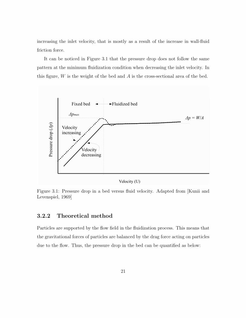
increasing the inlet velocity, that is mostly as a result of the increase in wall-fluid
friction force.
It can be noticed in Figure 3.1 that the pressure drop does not follow the same
pattern at the minimum fluidization condition when decreasing the inlet velocity. In
this figure, W is the weight of the bed and A is the cross-sectional area of the bed.
Figure 3.1: Pressure drop in a bed versus fluid velocity. Adapted from [Kunii andLevenspiel, 1969]
3.2.2 Theoretical method
Particles are supported by the flow field in the fluidization process. This means that
the gravitational forces of particles are balanced by the drag force acting on particles
due to the flow. Thus, the pressure drop in the bed can be quantified as below:
21

(3.1) 4 pA = H(1− εg)(ρs − ρg)g
Where 4p is the pressure drop, A is the cross-sectional area of the bed, H is
the bed height, εg is the bed porosity, and ρs and ρg are the solid density and fluid
density, respectively.
Ergun [1952] suggested that the pressure drop in a bed can be estimated as below:
(3.2)4p
4L= 150
(1− εg)2µgU
ε3gd2s
+ 1.75(1− εg)ρgU
2
ε3gds
In this equation µg is the gas viscosity and ds is the diameter of the particle.
Kunii and Levenspiel [1969] replaced the minimum fluidization condition pa-
rameters in the Ergun equation and derived Equation 3.3 for minimum fluidization
condition:
(3.3)1.75
φsε3g,mf
Re2mf +150(1− εg,mf )
φ2sε
3g,mf
Remf =d3sρg(ρs − ρg)g
µ2g
(3.4) Remf =dsUmfρg
µg
where subscript mf refers to minimum fluidization condition, and φs is the
sphericity of the particle which is defined as below:
22

(3.5) φs =
(surface of sphere
surface of particle
)both of same volume
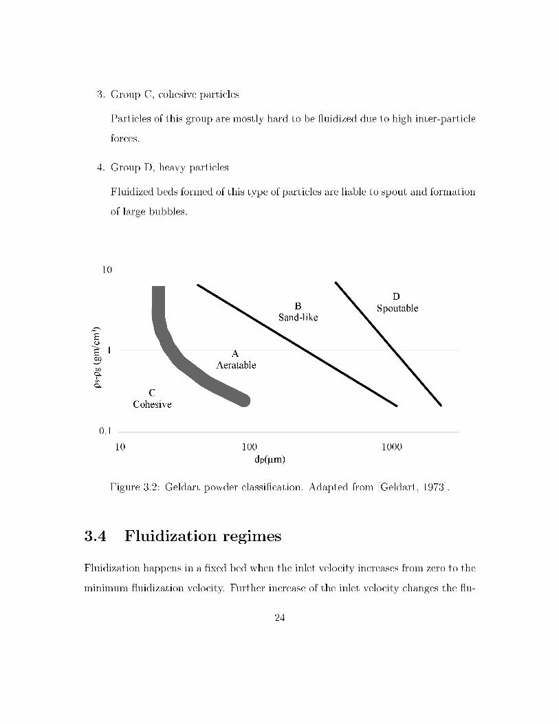
3.3 Solid particles classification
There are many factors affecting the solids behaviour in a fluidized bed, of which the
most important are:
1. Carrier phase density, ρg, and viscosity, µg;
2. Solid phase density, ρs;
3. Mean diameter of the particles, dp, and;
4. Particle shape, φs.
Figure 3.2 shows the classification of solid powders behavior (fluidized by gas)
based on the mean particles diameter and solid-gas density difference, which can be
described as follows [Geldart, 1973]:
1. Group A, aeratable particles
When a packed bed is formed by particles of group A, the bed expands, and
bubbles are formed later. Solids of the category are mixed vigorously.
2. Group B, sand-like particles
In a bed formed by particles of group B, large bubbles grow in the bed. The
size of these bubbles is controlled by the internal forces in the bed.
23
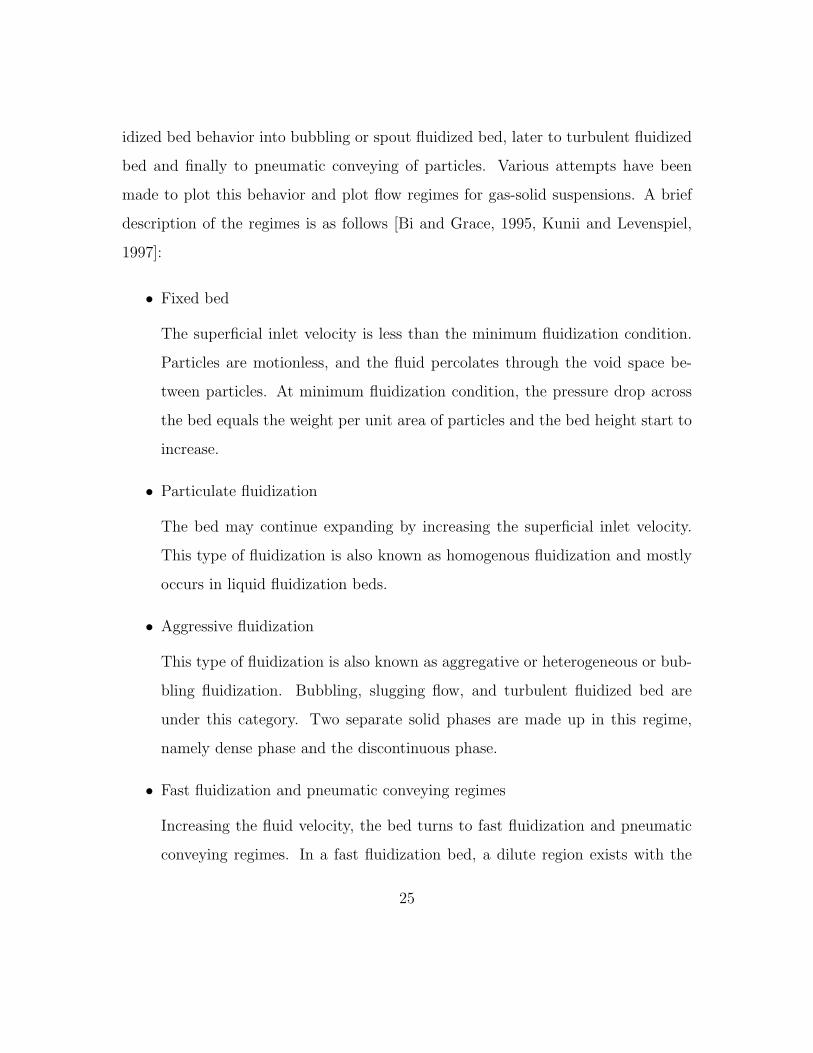
idized bed behavior into bubbling or spout fluidized bed, later to turbulent fluidized
bed and finally to pneumatic conveying of particles. Various attempts have been
made to plot this behavior and plot flow regimes for gas-solid suspensions. A brief
description of the regimes is as follows [Bi and Grace, 1995, Kunii and Levenspiel,
1997]:
• Fixed bed
The superficial inlet velocity is less than the minimum fluidization condition.
Particles are motionless, and the fluid percolates through the void space be-
tween particles. At minimum fluidization condition, the pressure drop across
the bed equals the weight per unit area of particles and the bed height start to
increase.
• Particulate fluidization
The bed may continue expanding by increasing the superficial inlet velocity.
This type of fluidization is also known as homogenous fluidization and mostly
occurs in liquid fluidization beds.
• Aggressive fluidization
This type of fluidization is also known as aggregative or heterogeneous or bub-
bling fluidization. Bubbling, slugging flow, and turbulent fluidized bed are
under this category. Two separate solid phases are made up in this regime,
namely dense phase and the discontinuous phase.
• Fast fluidization and pneumatic conveying regimes
Increasing the fluid velocity, the bed turns to fast fluidization and pneumatic
conveying regimes. In a fast fluidization bed, a dilute region exists with the
25
dense phase. Particles are carried by the fluid in the center and form the dilute
region while the dense regions are formed on the walls of the bed. Increas-
ing the inlet velocity, pneumatic conveying of particles starts, which can be
distinguished from the fast fluidization regime as the dense regions disappear,
replaced by a vertically uniform distribution of particles.
Figure 3.3 presents the model developed to describe the flow behavior based on
the particles size, density, sphericity, and fluid phase density and viscosity [Kunii
and Levenspiel, 1997]. This map of fluidization regimes will be useful to classify the
type of flow behavior of the simulations in this study.
26

Where
(3.6) d∗s = ds
[ρg(ρs − ρg)g
µ2g
]1/3
(3.7) u∗ = u
[ρ2g
µg(ρs − ρg)g
]1/3
and g is the gravity.
3.5 Multiphase modelling approaches
There are two main approaches to model the mixture behavior. One considers the
dispersed phase as a continuous phase and derives the equations based on a fluid
characteristic. This approach is called the Eulerian perspective and requires empirical
equations to model the behavior of the dispersed phase. On the other hand, the
Lagrangian perspective considers every single particle and derives the equations of
motions of the particles based on mass and velocity of the particles using Newton’s
laws of motion. The carrier phase in both approaches is treated as a continuous
phase, and locally averaged variables are utilized in the governing equations of the
carrier phase [Crowe et al., 2011].
3.5.1 Carrier phase governing equations
The carrier phase in Eulerian - Eulerian and Eulerian - Lagrangian approach is
treated as a continuous phase and equations of conservation of mass, momentum,
and energy for this phase are solved to model the carrier phase. A review of the
28

governing equations from the multiphase flows textbook by Crowe et al. [2011] is
presented here.
Continuity equation
According to the conservation of mass, summation of the rate of mass accumulation
and the net out-flux of mass should be zero.
Assuming there is no mass transfer and the fluid is incompressible the continuity
equation can be written in differential form for a multidimensional flow as below:
(3.8)∂
∂t(εgρg) +∇ · (εgρgu) = 0
Where u is the gas velocity.
Momentum equations
The conservation of momentum can be expressed as the summation of the rate of
change of momentum in the control volume and net out-flux of momentum from the
control volume, which is equal to the force on the fluid in the control volume.
For multidimensional flows, assuming there is no mass transfer, the momentum
equations can be rewritten in the following form:
(3.9)∂
∂t(εgρgu) +∇ · (εgρguu) = −εg∇pg +∇Tg + εgρgg + β(v − u)
In this equation β is the fluid-particle friction coefficient, v is the solid velocity
and the gas phase stress tensor, Tg, can be represented as:
29
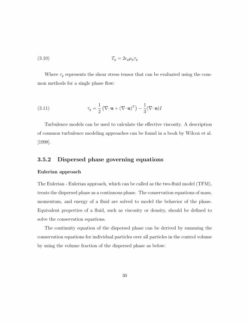
(3.10) Tg = 2εgµgτg
Where τg represents the shear stress tensor that can be evaluated using the com-
mon methods for a single phase flow:
(3.11) τg =1
2
(∇·u+ (∇·u)T
)− 1
3(∇·u)I
Turbulence models can be used to calculate the effective viscosity. A description
of common turbulence modeling approaches can be found in a book by Wilcox et al.
[1998].
3.5.2 Dispersed phase governing equations
Eulerian approach
The Eulerian - Eulerian approach, which can be called as the two-fluid model (TFM),
treats the dispersed phase as a continuous phase. The conservation equations of mass,
momentum, and energy of a fluid are solved to model the behavior of the phase.
Equivalent properties of a fluid, such as viscosity or density, should be defined to
solve the conservation equations.
The continuity equation of the dispersed phase can be derived by summing the
conservation equations for individual particles over all particles in the control volume
by using the volume fraction of the dispersed phase as below:
30
(3.12)∂
∂t(εsρs) +∇ · (εsρsv) = 0
The momentum equation for a cloud of particles can be derived by summing
conservation equations for individual particles in the control volume.
(3.13)∂(εsρsv)
∂t+∇ · (εsρsvv) = −εs∇Ps +∇Ts + εsρsg − β(v − u)
The solid phase stress tensor can be represented as below:
(3.14) Ts = (−Ps + ξs∇ · v)I + 2µsτs
In this equation PS is the solid phase pressure, ξs is the bulk viscosity, and µs
represents the shear viscosity. These variables can be defined as functions of the
granular temperature as well as the particle restitution coefficient, particle diameter,
material density, and particles volume fraction.
The granular temperature, Θ, is based on the kinetic theory of dense gasses, which
was first introduced by Bagnold [1954]. Later, Gidaspow [2012] used the granular
temperature of the dense flows to describe the particles’ velocity fluctuations, C, as
below:
(3.15) Θ =1
3〈C2〉
31
The conservation equation of the granular temperature is given as below:
(3.16)3
2
[∂
∂t(εsρsΘ) +∇ · (εsρsv ·Θ)
]= Ts : ∇v +∇ · v +∇ · k∇Θ− γ
where Ts : ∇v is the generation of the fluctuation energy due the work of the
shear stress in the particle phase, ∇·∇Θ is the conduction of the fluctuating energy
and γ is the dissipation of due to inelastic collisions. For more information about
TFM approach and kinetic theory, please refer to Gidaspow [2012].
As there is no need to consider every single particle dynamics in the two-fluid
model large systems can be modeled, which is the main advantage of this approach.
However, in a particular system with particle size distribution, a new phase should be
considered for each particle size or empirical models should be used, which increases
the complexity of the problem [Crowe et al., 2011].
Lagrangian approach
Governing equations
In the Eulerian - Lagrangian approach, the carrier phase is treated as a continuous
fluid, and the conservation equations are used to model it. Particles in the dispersed
phase are tracked individually or as parcels of particles in the flow field. Locally aver-
aged variables are employed in the conservation equations to be solved. Momentum
and mass transfer between the phases are permitted in these equations. Two mod-
els are proposed in the literature for the momentum equations formulation, namely
Model A and B [Gidaspow, 2012]. The Model A assumes that the pressure drop is
shared between the gas and solid phase, and the Model B assumes that the pressure
32
drop is applied to the gas phase only [Feng and Yu, 2004].
The continuity equation can be written as below:
(3.17)∂εg∂t
+∇· (εgu) = 0
The set of momentum conservation equations can be written as below:
• Model A
(3.18)∂ρgεgu
∂t+∇· (ρgεguu) = −εg∇P − FA +∇· (εgτ) + ρgεgg
• Model B
(3.19)∂ρgεgu
∂t+∇· (ρgεguu) = −∇P − FB +∇· (εgτ) + ρgεgg
In these sets of equations, FA and FB are the volumetric particle - fluid interaction
forces for the two models, and they are interchangeable using the following equation:
(3.20) FB =FA
εg− ρgεsg
On the dispersed phase side, the force acting on each particle is the summation
of the forces due to the contact force of particles, fc,ij + fd,ij , the force imposed by
the carrier phase, fp−f,i, and the gravity force as below:
33
(3.21) midup,i
dt= fp−f,i +
ki∑
j=1
(fc,ij + fd,ij) + ρp,iVp,ig
where Vp,i is the volume of the particle i and fp−f,i is the total particle - fluid
interaction force on the particle and is the summation of the drag force, the buoyancy
force, lifting force, the virtual mass force, Basset force, and others. fc,ij and fd,ij are
the contact force and the viscous contact damping forces respectively
The rotational momentum can be written as below:
(3.22) Iidωi
dt=
ki∑
j=1
Tij
Tij is the torque between particles i and j.
According to the models introduced for momentum equations of the carrier phase,
two models can be used to describe the particle - fluid interaction force, namely Model
A and B. Considering only the pressure drop and buoyancy terms these models can
be written as below:
Model A fp−f,i = −Vp,i∇pi + fA(3.23)
Model B fp−f,i = ρgVp,ig + fB(3.24)
In Model A, the buoyancy force is related to the pressure drop term, ∇pi, and
the other part, fA, is linked to the fluid drag force multiplied by the fluid volume
fraction, εgfdrag,i. In Model B the buoyancy force is related to the static pressure
34
drop, ∇p0, and the fluid drag force. It is good to notice that the total pressure drop,
∇P , consists of three factors in a bed [Feng and Yu, 2004]:
• The hydrostatic pressure drop, ∇p0, which is due to the gravity force of the
gas.
• The hydrodynamic pressure drop, ∇pd, which is due to the relative motion
between the gas and particles.
• The pressure drop due to the friction of the gas and the walls, ∇pw. This term
can be neglected compared to other terms of the total pressure drop.
Equations 3.23 and 3.24 can be rewritten in the following forms:
Model A fp−f,i = −Vp,iρgg + Vp,i∇pd,i + εgfdrag,i(3.25)
Model B fp−f,i = −Vp,iρgg + εsfdrag,i + εgfdrag,i(3.26)
When forming a uniform bed of mono-sized particles, where there is no accelera-
tion in either phase, the pressure drop is the summation of the static pressure drop,
∇p0, and the dynamic pressure drop, ∇pd. In this system, the point-wise values of
the pressure drop around each particle, ∇pd,i, are identical and can be replaced with
the locally averaged pressure drop value, ∇pd. The particle volume, Vp,i, is equal to
εs/n and the relation between the hydrodynamic pressure drop and the particle drag
force can be written as below[Feng and Yu, 2004] :
(3.27) ∇pd = nfdrag,i
The second term on the right hand side of Equation 3.25 can be written as below:
35
(3.28) Vp,i∇pd,i =εsnnfdrag,i
The Model A and B predict the same results for a packed bed of monosized
particles. However, this concept is not applicable in the fluidization process, and
Model A and B predict different results. This difference is because in Model A a
point-wise value of the pressure drop around each particle is needed, ∇pd,i, while
just locally averaged pressure drop value can be obtained through the continuum
approach. In the fluidization process particles are not uniformly distributed in space
and their velocity and trajectories are not the same. The non-uniform particle cloud
results in a difference between the locally averaged pressure drop and the point-wise
value of the pressure drop around each particle [Feng and Yu, 2004].
Particle - fluid interactions
The coupling of the forces between the dispersed phase and the carrier phase can be
derived according to the Newton’s third law of motion. The force of the dispersed
phase acting on the gas phase should be equal to the force of the gas phase working
on the dispersed phase but in the opposite direction. To achieve this relation three
schemes are presented in the literature [Feng and Yu, 2004, Gidaspow, 2012]:
• The first scheme calculates the forces from particles to the gas phase by the
local average method, and forces from the gas phase to the solid phase are cal-
culated separately according to the individual particle velocity. The conditions
of Newton’s third law of motion are not guaranteed in this scheme.
• The second scheme calculates forces from particles to the gas phase at local-
36
average scale as used in scheme one, and then distributes the estimated values
between individual particles according to certain averaging rules. For a mono-
sized particle system the following relation can be derived according to this
scheme:
(3.29) f =F∇V
kc
where kc is the number of particles in the computational cell, ∇V is the volume
of the CV and F is the volumetric particle-fluid interaction force.
This scheme can satisfy the Newton’s third law of motion. However, this
method distributes the interaction force between the particles uniformly, and
does not consider the different trajectories and velocities of the particles. Be-
sides, it is necessary to use a mean particles’ velocities to calculate the inter-
action force, F. The appropriate method of estimation of the mean particles’
velocities is still an open topic.
• Xu and Yu [1997] introduced the third scheme, which calculates the particle -
fluid interaction force at each time step on individual particles in a computa-
tional cell, and then calculates the summation of these values to produce the
particle - fluid interaction force at the cell scale. The following equation can
be used for this scheme:
(3.30) F =
∑kci=1 f
∇V
37
This scheme can overcome problems mentioned for scheme 1 and 2, and is
widely used by researchers [Feng and Yu, 2004] .
The effect of particle cloud on the drag coefficient is still an open topic. Numerical
methods such as Direct Numerical Simulation (DNS) and Lattice Boltzmann (LB)
have been used to quantify the drag force from fluid to a particle in a particle cloud.
However, these studies are mostly limited to simple geometries and cases due to their
high demand of computational power. Therefore, calculation of the interaction force
of the fluid to the particles, f, in the current work is based on the calculation of
pressure drop using available models in the literature, namely Model A and B [Feng
and Yu, 2004, Gidaspow, 2012].
The hydrodynamic pressure drop is assumed to be shared uniformly between
particles in Model A and B. The following models can be derived for each set of
momentum equation [Feng and Yu, 2004]:
1. Model A
(3.31) fA =εgn∇pd =
π
6d3i
εgεs∇pd
2. Model B
(3.32) fB =∇pdn
=π
6d3i
1
εs∇pd
The drag force is the main interaction force in a gas-solid system. The drag force
on an isolated particle in a flow field can be written as below Crowe et al. [2011]:
38
(3.33) F =1
2ρgCDAp|u− v|(u− v)
Where CD is the drag coefficient, and Ap is the area of the particle. The drag
factor is the ratio of the drag coefficient to the Stokes drag, which is introduced as:
(3.34) f =CDRer24
and
(3.35) Rer =ρg|u− v|r
µg
The drag force on an isolated sphere in the flow is a well-known problem. Re-
searchers have developed many models to quantify drag on a sphere [Haider and
Levenspiel, 1989, Putnam, 1961, Schiller and Naumann, 1935]. However, there is not
enough information on the effect of the particle cloud on the drag coefficient. Numer-
ical and experimental works have been done to study the effect of particle cloud on
the drag coefficient. The drag force on particles in a bed formed of multi-sized parti-
cles is still and open topic [Feng and Yu, 2004]. However, equations of pressure drop
and drag force for monosized systems are used for multi-sized beds as well. Different
models are presented in the literature for the drag force of a particle in particle cloud
as the friction coefficient as explained next [Crowe et al., 2011, Gidaspow, 2012]:
According to Darcy’s law the pressure drop can be related to the friction coeffi-
cient, β, as below Gidaspow [2012]:
39

(3.36) − εg∂p
∂x− β(u− v) = 0
• Ergun [1952]
Based on the Ergun equation of pressure drop, Equation 3.2, the friction coef-
ficient can be written as below:
(3.37) β = 150ε2sµg
εg(dφs)2+ 1.75
ρg|u− v|εsφsd
• Wen and Yu [1966]
Wen and Yu [1966] suggested a correction to Richardson and Zaki [1954] equa-
tion of the pressure drop, when the porosity is greater than 0.8 and derived the
following equation for the friction coefficient:
(3.38) β =3
4CD
εgεs|u− v|ρgd
f(εg)
where CD is the drag coefficient of an isolated particle as below:
CD =24
Res
(1 + 0.15(Res)
0.687), Res < 1000
CD = 0.44, Res ≥ 1000(3.39)
40
where Res is as follows:
(3.40) Res =εgρg(|u− v|)d
µg
and f(εg) is a correction for presence of the particle cloud and is given as below:
(3.41) f(εg) = ε3.7g
• Gidaspow [2012]
Gidaspow [2012] suggested that the drag model proposed by Ergun [1952],
Equation 3.37, is valid for dense flows, when εg < 0.8, and to use Wen and Yu
[1966] drag model, Equation 3.38, for dilute flows, when εg is greater than 0.8,
with a correction as below:
(3.42) f(εg) = ε−2.65g
• Di Felice [1994]
Di Felice [1994] found by analysis of published data a correction for f(εg) and
suggested the following equation:
(3.43) f(εg) = ε−ξg
41

where ξ is the following empirical equation:
(3.44) ξ = 3.7− 0.65 exp
[−(1.5− log(Rer))
2
2
], 10−2 < Rer < 104
• Koch and Hill [2001]
Koch and Hill [2001] developed a model for drag coefficient of a particle in
particle cloud based on Lattice - Boltzmann method as below:
F0 =
1+3√
εs/2+(135/64)εsln(εs)+16.14εs
1+0.681εs−8.48ε2s+8.16ε3s, εs < 0.4
10εs(1−ε3s)
, εs > 0.4(3.45)
(3.46) F3 = 0.0673 + 0.212εs +0.0232
(1− εs)5
(3.47) F = F0 +F3Re
2
(3.48) βp =18µg(1− εs)
2ε2sF
d2s
42
(3.49) Re =ρgεs|u− v|ds
µg
(3.50) Fp,f =Vpβp
εs(u− v)
Particle - particle interactions
The Hard Sphere Model (HSM) or the Soft Sphere Model (SSM) can be used to
model the total particles’ interactions forces in Lagrangian approach. An overview
of the models is presented below. Further explanation of the models can be found
in [Crowe et al., 2011].
1. Hard Sphere Model (HSM)
HSM is based on the impulsive forces, which are defined by the integral of the
forces acting on a particle versus time. In this approach particles are assumed
to be rigid without any deformation.
Three assumptions are made for HSM:
(a) particle deformation is negligible;
(b) the friction on sliding particles obeys Coulomb’s friction law;
(c) once a particle stops sliding there is no further sliding.
2. Soft Sphere Model (SSM)
The soft-sphere model assumes an overlap displacement δ to consider the de-
formation of the particles as they collide. This displacement distance is shown
43

in Figure 3.4. A frictional force is resulted when particles collide and are de-
formed. This force is generated because of the presence of the normal collision
force. Particles’ tangential and normal forces of the collisions are calculated
by using the spring, dashpot and friction slider mechanical elements. Figure
3.5 presents a schematic of these elements. In this model, the relation between
pre-collision and post-collision velocities can be obtained. Also, forces acting
on particles during the contact period are calculated.
Figure 3.4: Displacement of two particles in contact. Adapted from [Crowe et al.,2011]
Forces acting on particles can be calculated using Equation 3.51 for the normal
force and Equation 3.52 for the tangential force.
44
The normal component of the contact force is the summation of the spring and
the dashpot forces:
(3.51) Fnij = (knδn − ηnjG · n)n
And the tangential component of the contact force is the summation of the
slider, spring and the dash-pot forces:
(3.52) Ftij = −ktδt − ηtjGct
where G is the relative velocity of the particles and defined as below:
(3.53) G = vi − vj
and Gct is the slip velocity at the contact point, which is given by:
(3.54) Gct = G− (G · n)n+R∗(ωi + ωj)× n
By assuming the second particle’s diameter to be infinite, particle - wall colli-
sion equations can be derived.
Three parameters should be defined for this model:
45
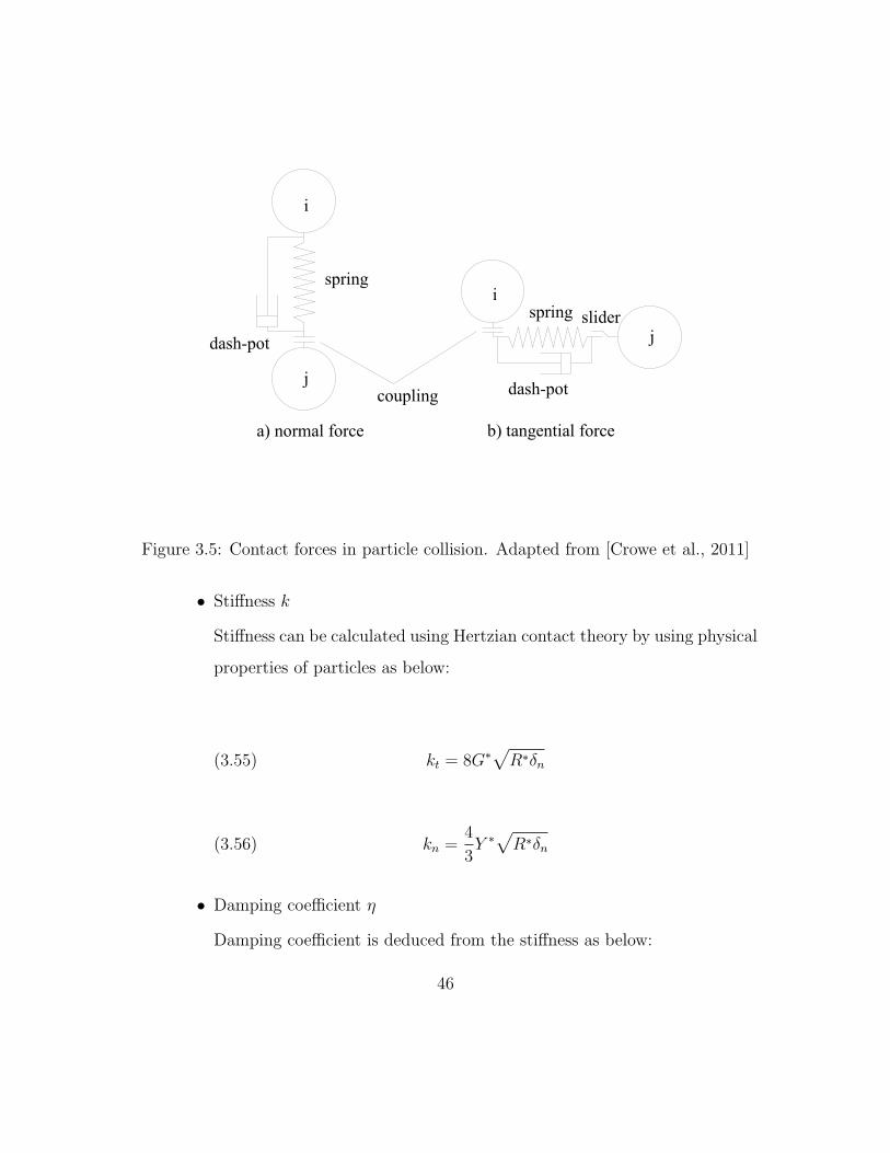
Figure 3.5: Contact forces in particle collision. Adapted from [Crowe et al., 2011]
• Stiffness k
Stiffness can be calculated using Hertzian contact theory by using physical
properties of particles as below:
(3.55) kt = 8G∗√
R∗δn
(3.56) kn =4
3Y ∗
√R∗δn
• Damping coefficient η
Damping coefficient is deduced from the stiffness as below:
46
(3.57) ηn = −2
√5
6β√Snm∗
(3.58) ηt = −2
√5
6β√Stm∗
• friction coefficient f
Friction coefficient is measurable and can be described by an empirical
value.
In these equations Y ∗, G∗, R∗, β and S are defined as below:
(3.59)1
Y ∗=
1− ν21
Y1
+1− ν2
2
Y2
(3.60)1
G∗=
2(2 + ν1)(1− ν1)
Y1
+2(2 + ν2)(1− ν2)
Y2
(3.61)1
R∗=
1
r1+
1
r2
47
(3.62) β =ln(e)√
ln2(e) + π2
(3.63) Sn = 2Y ∗√
R∗δn
(3.64) St = 8G∗√
R∗δn
In the above equations, Y is the Young modulus of the particle, G is the shear
modulus, ν is the Poisson ratio, e is the coefficient of restitution, m is the mass
of the particle, and r is the radius of the particle.
The total force acting on particle i is the summation of the tangential and normal
forces of particles which are in contact with particle i and is written as below:
(3.65) Fi =∑
j
(Fnij + Ftij)
And the torque can be calculated using summation of torques imposed to the
particle i by tangential component of the contact force:
(3.66) Ti =∑
j
(Rin× Ftij)
48


• Trajectory segregation
According to the drag force on a sphere the retarding force on a particle is pro-
portional to the square of its diameter, f = 12ρgU
2Cd(πd2s4), and the deceleration
of the particle can be calculated as below:
(3.67) Deceleration of the particle =retarding force
mass of particle
The travel distance of a particle to settle is proportional to the square of its
diameter. Therefore, a particle of twice the diameter would move four times
the distance to settle, which results in segregation of particles with different
size. This method is used in a conveying belt mostly.
• Percolation of particles
Particles of the same size tend to aggregate in a moving mass of particles.
This movement trend leads to creation of a gap between the particles so that a
smaller particle moves downward while a larger one moves upward. This mech-
anism mostly occurs in hoppers during charging and discharging of particles.
• Rise of coarse particles due to vibrations
Vibrations in a mixture of particles of different size can cause segregation.
Larger particles would travel upward while smaller particles move downward.
• Elutration segregation
At the presence of an upward flow in a cylinder, particles with terminal ve-
locities lower than the upward flow velocity are carried upward and heavier
particles are settled.
50
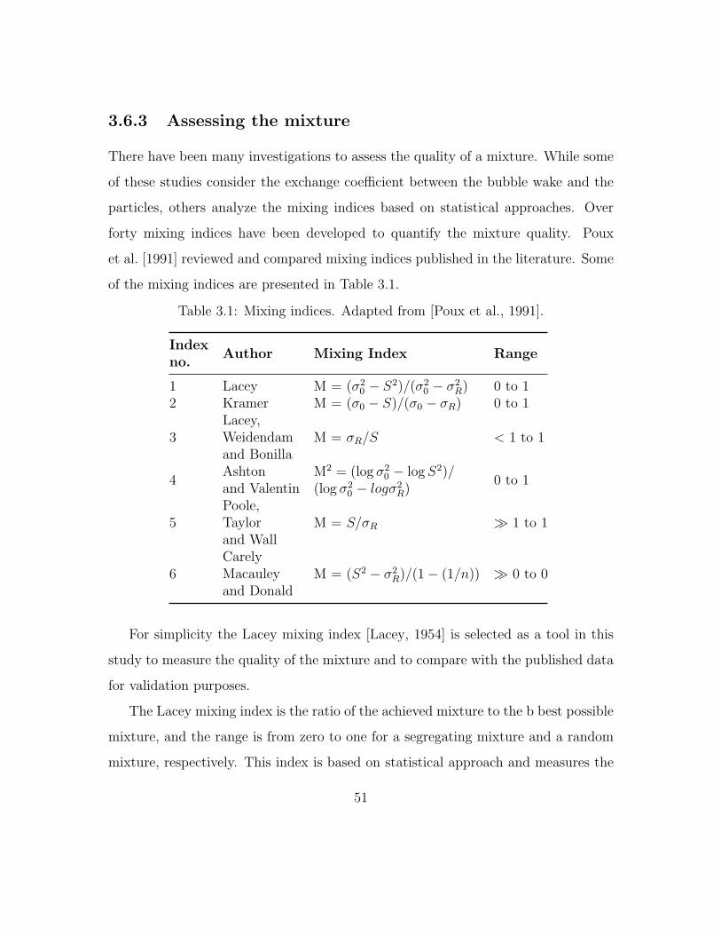
3.6.3 Assessing the mixture
There have been many investigations to assess the quality of a mixture. While some
of these studies consider the exchange coefficient between the bubble wake and the
particles, others analyze the mixing indices based on statistical approaches. Over
forty mixing indices have been developed to quantify the mixture quality. Poux
et al. [1991] reviewed and compared mixing indices published in the literature. Some
of the mixing indices are presented in Table 3.1.
Table 3.1: Mixing indices. Adapted from [Poux et al., 1991].
Indexno.
Author Mixing Index Range
1 Lacey M = (σ20 − S2)/(σ2
0 − σ2R) 0 to 1
2 Kramer M = (σ0 − S)/(σ0 − σR) 0 to 1
3Lacey,Weidendamand Bonilla
M = σR/S < 1 to 1
4Ashtonand Valentin
M2 = (log σ20 − log S2)/
(log σ20 − logσ2
R)0 to 1
5Poole,Taylorand Wall
M = S/σR � 1 to 1
6CarelyMacauleyand Donald
M = (S2 − σ2R)/(1− (1/n)) � 0 to 0
For simplicity the Lacey mixing index [Lacey, 1954] is selected as a tool in this
study to measure the quality of the mixture and to compare with the published data
for validation purposes.
The Lacey mixing index is the ratio of the achieved mixture to the b best possible
mixture, and the range is from zero to one for a segregating mixture and a random
mixture, respectively. This index is based on statistical approach and measures the
51

degree of the mixture using the variation of compositions among samples drawn out
of the mixture, σ2.
The standard deviation of a completely random mixture, composed of particles
of the same size, σ2R, is calculated as below:
(3.68) σ2R =
P (1− P )
n
where P is the overall portion of any component of the mixture and n is the
number of particles in each sample.
The standard deviation of a segregating mixture, composed of mono-sized parti-
cles, can be estimated as below:
(3.69) σ20 = P (1− P )
which is independent of the sample size.
The standard deviation of a mixture samples can be estimated as below:
(3.70) S2 =1
n
n∑
i=1
(xi − x)2
where x is the sample arithmetic mean defined as below:
(3.71) x =1
n
n∑
i=1
xi
52
Chapter 4
Numerical method
The name CFD refers to the use of numerical methods and a computer, or comput-
ers, to model the fluid dynamics of a desired flow. In this method partial differential
equations (PDE) and ordinary differential equations (ODE) forming the governing
equations are approximated and numerical schemes are used to solve them. Dis-
cretization methods should be used to approximate the solution of differential equa-
tions by use of an equivalent system of algebraic equations. Three main methods
are introduced in the literature for the discretization procedure [Ferziger and Peric,
2002]:
1. Finite difference method (FDM)
FDM discretizes the domain into nodes and solves the differential equations for
each node based on the neighboring nodes. The method is very straightforward
and efficient on structured grids. However, the implementation of the method
to complex flows and geometries is complex and conservation in not enforced
unless special care is taken [Ferziger and Peric, 2002].
2. Finite element method (FEM)
53
FEM breaks the domain into a set of discrete volumes or finite elements, which
are mostly unstructured. The differential equations are multiplied by weight
functions before they are integrated over the entire domain. One of the simplest
approximations to the solution over each element is the linear approximation
constructed from the value of the boundaries. This approximation guarantees
the continuity. This estimate is then multiplied by a weight function, which is
mostly the same form of the solution. This approximation is then submitted
into the weighted integral of the conservation law and by selecting the best
solution from the set of allowed functions, which corresponds to the one with
minimum residual, the final solution is found. This method satisfies the con-
servation and can be used for complex geometries by using unstructured grids
[Ferziger and Peric, 2002].
3. Finite volume method (FVM)
FVM divides the domain into a finite number of contiguous control volumes
(CV) and solves the integral form of the conservation equations at the centroid
of each CV. Interpolation methods are used to calculate the variables at the
surface of each CV. The method uses both structured and unstructured grids,
so it is suitable for complex geometries. Also, this method is conservative by
considering the in-flux and out-flux of variables at the boundaries, and the
rate of changes inside each CV. However, it is difficult to develop methods of
orders higher than second for 3D domains compared to FEM, because FVM
requires three levels of approximation: interpolation and integration [Ferziger
and Peric, 2002].
A non-linear algebraic system of equations can be developed by using any of the
methods mentioned above. Then, iterative methods are used to solve the system of
54
equations as below [Ferziger and Peric, 2002]:
Ax = b(4.1)
ε = Ax− b(4.2)
where A is the matrix of coefficients, x is the variable vector, b is the source term
vector and ε is the vector of iterations residual.
Following software packages are used to solve the discretized equations derived
in Chapter 3:
• OpenFOAM ® 2-3-0
OpenFOAM ® (Open Field Operation and Manipulation) is a free, open source
CFD package developed by OpenCFD Ltd. at ESI Group and is distributed
by the OpenFOAM Foundation. The software is coded in C++ programming
language and benefits from the modularity and object oriented features of
C++. This feature enables the software to the development of customized
numerical solvers and pre-/post processing utilities for CFD [Weller et al.,
1998]. OpenFOAM is based on FVM and solves PDEs and ODEs.
• LIGGGHTS® - Public
LIGGGHTS® (LAMMPS Improved for General Granular and Granular Heat
Transfer Simulations) is an open source software package for modeling granu-
lar material by the implementation of discrete element method (DEM) [Kloss
et al., 2012]. LIGGGHTS® is based on LAMMPS® (Large Atomic and Molec-
ular Massively Parallel Simulator), which is an open source software package
developed by Sandia National Laboratories for Molecular dynamics simulations
55
on distributed memory machines [Plimpton, 1995]. LIGGGHTS is based on
FDM and solves ODEs.
• CFDEM® coupling - 2.3.0
CFDEM® coupling (Computational Fluid Dynamics - Discrete Elements Method
coupling) is an open source software package developed mainly by DCS Com-
puting and is a modular framework which couples and transfers data between
CFD code and the DEM code using the particle - fluid interactions and volume
fraction [Goniva et al., 2012].
4.1 Solver: cfdemSolverPiso
cfdemSolverPiso is a coupled CFD-DEM solver, which couples the CFD solver, piso-
Foam, to the DEM engine, LIGGGHTS. The CFD solver uses the volume averaged
Navier-Stokes equations for the continuous phase and the DEM engine solves New-
ton’s equations of motion for the dispersed phase. The coupling code calculates
forces on the particles due to the flow field and transfers them to the DEM engine,
LIGGGHTS, where the trajectory and position of particles are calculated and up-
dated in the CFD solver. The pisoFoam is a finite volume based solver for unsteady,
incompressible, and turbulent flows, which uses the PISO algorithm, first introduced
by Issa [1986].
4.1.1 Governing equations
Following the description of the physics of the problem in Chapter 3.5.2, a summary
of the equations which are used in this study are presented in Table 4.1.
56
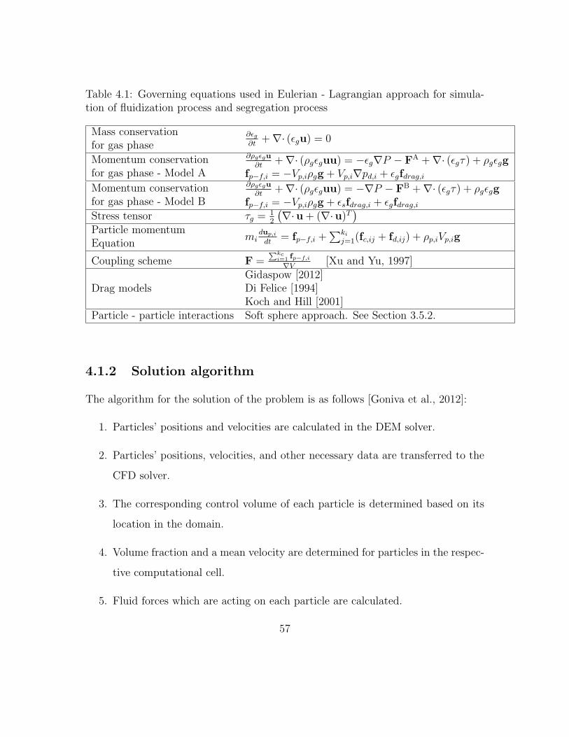
Table 4.1: Governing equations used in Eulerian - Lagrangian approach for simula-tion of fluidization process and segregation process
Mass conservationfor gas phase
∂εg∂t
+∇· (εgu) = 0
Momentum conservationfor gas phase - Model A
∂ρgεgu
∂t+∇· (ρgεguu) = −εg∇P − FA +∇· (εgτ) + ρgεgg
fp−f,i = −Vp,iρgg + Vp,i∇pd,i + εgfdrag,iMomentum conservationfor gas phase - Model B
∂ρgεgu
∂t+∇· (ρgεguu) = −∇P − FB +∇· (εgτ) + ρgεgg
fp−f,i = −Vp,iρgg + εsfdrag,i + εgfdrag,iStress tensor τg =
12
(∇·u+ (∇·u)T
)
Particle momentumEquation
midup,i
dt= fp−f,i +
∑kij=1(fc,ij + fd,ij) + ρp,iVp,ig
Coupling scheme F =∑kc
i=1fp−f,i
∇V[Xu and Yu, 1997]
Drag modelsGidaspow [2012]Di Felice [1994]Koch and Hill [2001]
Particle - particle interactions Soft sphere approach. See Section 3.5.2.
4.1.2 Solution algorithm
The algorithm for the solution of the problem is as follows [Goniva et al., 2012]:
1. Particles’ positions and velocities are calculated in the DEM solver.
2. Particles’ positions, velocities, and other necessary data are transferred to the
CFD solver.
3. The corresponding control volume of each particle is determined based on its
location in the domain.
4. Volume fraction and a mean velocity are determined for particles in the respec-
tive computational cell.
5. Fluid forces which are acting on each particle are calculated.
57

6. Particle - fluid interaction forces and momentum exchange are assembled by
using the ensemble averaging method over all particles in a CFD cell.
7. Forces on the particles due to the flow field are transferred to the DEM solver
to be used in the next time step.
8. Fluid velocity and pressure are calculated in CFD cells and particles are rep-
resented by the volume fraction and momentum exchange term.
9. Additional equations are solved for both phases, such as heat transfer and
species transfer.
10. The routine is repeated from (1).
The gas phase solver, pisoFoam, is based on the pressure implicit with splitting
of operator (PISO) algorithm first introduced by Issa [1986], which is as below:
1. Set the boundary conditions.
2. Use the velocity and pressure fields from the previous time step, (un) and (pn),
or initial condition as an immediate estimate for the current time step.
3. Calculate an estimate for the current time step velocity (um∗) field by solving
the linearized momentum equation.
4. Solve the pressure correction equation to obtain the pressure correction term
(p′).
5. Correct the velocity and pressure fields by using the pressure correction term
and find the velocity (um) and pressure (pm) fields which satisfy the continuity
equation.
58

6. Solve the second pressure correction equation and correct the velocity (um) and
pressure (pm) fields again.
7. Repeat from 3 using the corrected velocity (um) and pressure (pm) fields as the
improved estimations until all corrections are negligible and store the latest
values for velocity and pressure fields as (un+1) and (pn+1) respectively.
8. Increase the time step and repeat from step 1 [Ferziger and Peric, 2002].
Particles’ force balances and their trajectories are calculated using Newton’s law
of motion in LIGGGHTS. LIGGGHTS is based on LAMMMPS, which uses the fast
parallel algorithm for short-range molecular dynamics developed by Plimpton [1995]
as below:
1. A list of non-zero interacting neighboring pairwise particles is generated.
2. Interaction forces, Fx are calculated for each pairwise particles and summations
of the forces are stored in the force matrix, fx.
3. New position of particles are computed by using the force balance of each
particle, fx, and then they are stored in the position matrix, xx.
4.1.3 File structure
CFDEM ® coupling and OpenFOAM ® use the dictionary files to define the param-
eters of the simulation. Dictionary files are created in the simulation run folder under
two main sub-folders, namely CFD and DEM. The CFD folder contains information
related to the gas phase, geometry and the grid of the gas phase simulation, and the
DEM folder includes information required by LIGGGHTS for calculation of parti-
cles’ force balance and positions, such as particle diameter, density, properties and
59

simulation domain properties. Figure 4.1 presents a schematic of the file structure
of the simulation setup.
4.2 Model setup
The workbench experiment developed by Feng and Yu [2004] is used in the current
work to model the fluidization and segregation process in the fluidized bed. Re-
sults are compared for verification and validation purposes. Figure 4.2 presents a
schematic of the geometry, mesh and initial conditions of the model.
4.2.1 Geometry
A rectangular bed, width = 65 mm, height = 260 mm and depth = 8.1 mm, is used
in the simulation to study the fluidization and segregation process in the fluidized
bed.
4.2.2 Mesh
The domain is discretized into structured hexahedral control volumes. Grid sensi-
tivity analysis is performed to study the effect of the grid size on the simulations’
results.
4.2.3 Boundary conditions
Velocity inlet boundary condition is used for the inlet considering the volume fraction
of the gas phase to be one and for particles to be zero, so that just air is injected
at the inlet. The effect of the inlet velocity is studied by considering different inlet
velocities and comparing to the minimum fluidization velocity of the jetsam particles.
60

Figure 4.1: CFDEM ® coupling file structure.
61
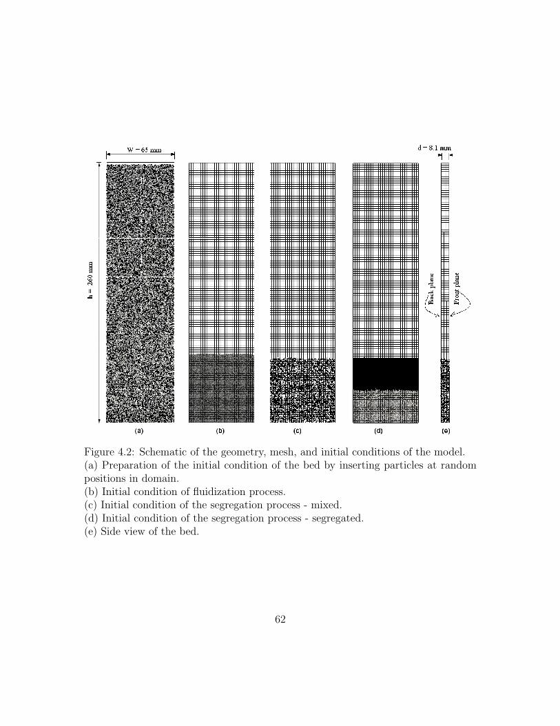
Figure 4.2: Schematic of the geometry, mesh, and initial conditions of the model.(a) Preparation of the initial condition of the bed by inserting particles at randompositions in domain.(b) Initial condition of fluidization process.(c) Initial condition of the segregation process - mixed.(d) Initial condition of the segregation process - segregated.(e) Side view of the bed.
62
Pressure outlet is used at the outlet, using a value of zero relative pressure.
Particle volume fractions at the outlet are set to zero, so that particles cannot leave
the domain.
Slip wall is used for the gas phase on the side walls. The implementation of
locally averaged variables does not allow the no-slip boundary conditions for walls
[Anderson and Jackson, 1967]. Hertzian walls with the coefficient of restitution of
0.9 are considered for the solid phase.
The effect of front and back planes on the results of simulations is studied by
considering periodic and slip wall boundary conditions for the gas phase and periodic,
frictional wall, and ideal wall for the dispersed phase.
4.2.4 Materials
Air at -50℃ is used as the gas phase and sand is used as the particles. Later, bitumen
pellets at -50℃ are added to study the segregation process. Properties of phases are
set according to suggested values in the literature. See Table 5.1 for an overview of
properties.
4.2.5 Numerical schemes
The numerical schemes used in a simulation play an important role in the results of
the simulations. Following schemes are used for discretization of equations terms:
• First order implicit Euler is used for temporal discretization.
• The divergence terms are estimated by Gaussian scheme with limited linear
interpolation scheme.
• The Laplacian terms are estimated by Gaussian scheme with linear correction.
63
• The linear interpolation scheme is used as default for all terms, otherwise men-
tioned.
See Appendix A for the complete dictionary of the numerical schemes and explana-
tions.
4.2.6 Initial conditions
The packed bed is formed by inserting 40,000 particles at random positions without
overlap in the whole domain when the internal fluid velocity is set to zero. The
particles are settled down due to the gravity force.
To study the effect of the initial condition on the segregation process, two dif-
ferent initial conditions are considered namely, initially mixed and initially inverse
segregated. In the initially mixed case, flotsam and jetsam particles are inserted at
random positions simultaneously to create a fully mixed bed as the initial condition,
and a packed bed with Lacey mixing index of one is generated (see Figure 4.2c). The
inverse segregated packed bed is formed by adding flotsam particles in a box lower
than the jetsam. A packed bed containing two distinct layers of flotsam and jetsam
is formed of which the Lacey mixing index is estimated to be zero (see Figure 4.2d).
4.2.7 Computational method
CFDEM ® coupling uses domain decomposition method for parallelization. The
domain is transferred to OpenFOAM for simulation of the continuous phase where
it is decomposed into sub-domains. Each CPU core is dedicated to one of the sub-
domains for calculations. The DEM engine is responsible for calculations of the
dispersed phase by using the fast parallel algorithm for short-range molecular dy-
64
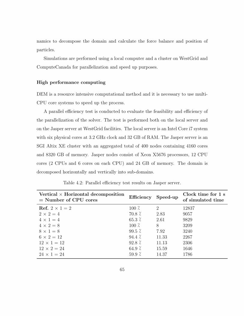
namics to decompose the domain and calculate the force balance and position of
particles.
Simulations are performed using a local computer and a cluster on WestGrid and
ComputeCanada for parallelization and speed up purposes.
High performance computing
DEM is a resource intensive computational method and it is necessary to use multi-
CPU core systems to speed up the process.
A parallel efficiency test is conducted to evaluate the feasibility and efficiency of
the parallelization of the solver. The test is performed both on the local server and
on the Jasper server at WestGrid facilities. The local server is an Intel Core i7 system
with six physical cores at 3.2 GHz clock and 32 GB of RAM. The Jasper server is an
SGI Altix XE cluster with an aggregated total of 400 nodes containing 4160 cores
and 8320 GB of memory. Jasper nodes consist of Xeon X5676 processors, 12 CPU
cores (2 CPUs and 6 cores on each CPU) and 24 GB of memory. The domain is
decomposed horizontally and vertically into sub-domains.
Table 4.2: Parallel efficiency test results on Jasper server.
Vertical × Horizontal decomposition= Number of CPU cores
Efficiency Speed-upClock time for 1 sof simulated time
Ref. 2 × 1 = 2 100 � 2 128372 × 2 = 4 70.8 � 2.83 90574 × 1 = 4 65.3 � 2.61 98294 × 2 = 8 100 � 8 32098 × 1 = 8 99.5 � 7.92 32406 × 2 = 12 94.4 � 11.33 226712 × 1 = 12 92.8 � 11.13 230612 × 2 = 24 64.9 � 15.59 164624 × 1 = 24 59.9 � 14.37 1786
65
The CFDEM®coupling is designed based on Message Passing Interface (MPI),
and at least two CPU cores are required to run in parallel mode. The simulation
time of a run with two CPU cores is used as the reference and simulation times are
compared with it. Table 4.2 shows parallel efficiency test results. The Jasper sever
uses the qsub and torque softwares to schedule jobs. According to their policy CPU
cores and nodes are assigned to the jobs based on the job request. A node consisted
of Intel Xeon L5420 might be assigned to a job which requests less than 8 CPU
cores. As it can be observed in Table 4.2 the efficiency of cases with four CPU cores,
a linear speed up was not gained. However, a good scaling was achieved up to 12
CPU cores. For the simulations with 24 CPU cores the speed up of the simulation
did not increase linearly. This is mainly because of running simulations on two nodes
rather than one node.
The speed-up for the reference test is considered to be 2 and for the other cases
the speed-up is defined as below:
(4.3) Speed-up =Clock time for the Reference test
Clock time for the case× 2
The efficiency of the reference test in considered to be 100% and for the other
cases the efficiency is defined as below:
(4.4) Efficiency =Speed-up
Number of CPU cores× 100
66
Chapter 5
Simulation of fluidization process
Air-sand fluidization is simulated as the first step to ensure the model is capturing
the hydrodynamics of the fluidized bed. Results of these two-phase simulations are
compared with published data. The third phase, bitumen, will be added later to
study the segregation process. The pressure drop is estimated along the bed as a
response variable and the particles’ mean velocity is used as the second response
variable. Both response variables are sensitive to the entire flow field within the
fluidized bed and, therefore, are good solution indicators.
As it was discussed in Chapter 2, proper grid size is a significant factor in pre-
diction of the bed hydrodynamics. To satisfy the volume average continuity and
momentum equations which are introduced by Anderson and Jackson [1967], the
minimum grid size is limited to be larger than the particles diameter in each direc-
tion [Muller et al., 2009].
Proper boundary conditions are required for a well-posed problem. Periodic and
wall boundary conditions are considered to study the effect of the boundary condi-
tions on the flow behavior.
67

The effect of drag models and momentum exchange models on the simulation
results are examined and the simulation settings are set accordingly. The response
variables (pressure drop along the bed and particles’ mean velocity) are used to
compare results with the results of previous works.
5.1 Reference simulation run
The reference simulation properties and settings are presented in Table 5.1.
Table 5.1: Reference simulation run setup
Description Value Comment
Gas density (kg m−3) 1.534 Air at -50℃
Gas viscosity (m2s−1 ) 9.55e-6 Air at -50℃
Particle density (kg m−3) 2500 Sand density
Particle diameter (mm) 1 Constant
Particle Young’s modulus (Nm−2) 1.0 × 10⁷ Feng and Yu [2004]
Particle Poisson ratio (N m−1) 0.33 Feng and Yu [2004]
Particle restitution coefficient 0.9 Feng and Yu [2004]
Particle friction coefficient 0.3 Feng and Yu [2004]
Bed size (w × h × d (m)) 0.065 × 0.26 × 0.0081 Feng and Yu [2004]
Static bed height (m) 0.065 40,000 particles
Inlet conditions
ug = 0.9 m s−1
us = 0 m s−1
∂∂np = 0
εg = 1
Velocity inlet
ug ∼ 1.5 umf
68
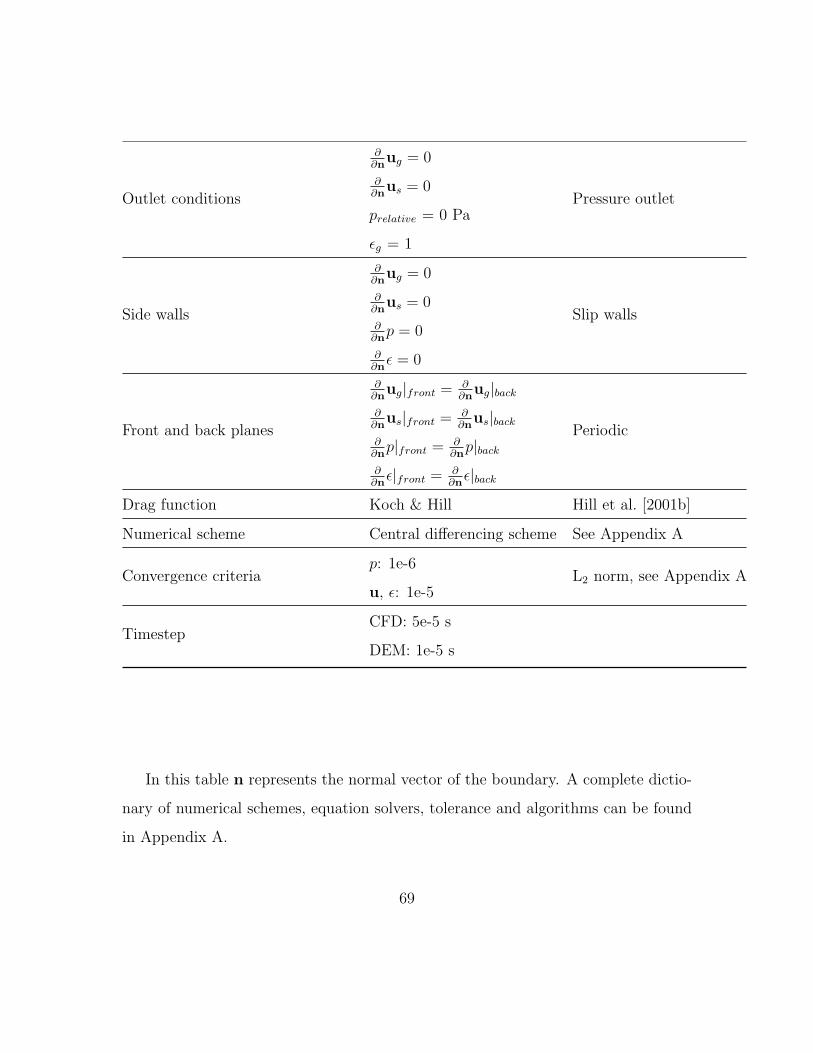
Outlet conditions
∂∂nug = 0
∂∂nus = 0
prelative = 0 Pa
εg = 1
Pressure outlet
Side walls
∂∂nug = 0
∂∂nus = 0
∂∂np = 0
∂∂nε = 0
Slip walls
Front and back planes
∂∂nug|front = ∂
∂nug|back
∂∂nus|front = ∂
∂nus|back
∂∂np|front = ∂
∂np|back
∂∂nε|front = ∂
∂nε|back
Periodic
Drag function Koch & Hill Hill et al. [2001b]
Numerical scheme Central differencing scheme See Appendix A
Convergence criteriap: 1e-6
u, ε: 1e-5L2 norm, see Appendix A
TimestepCFD: 5e-5 s
DEM: 1e-5 s
In this table n represents the normal vector of the boundary. A complete dictio-
nary of numerical schemes, equation solvers, tolerance and algorithms can be found
in Appendix A.
69
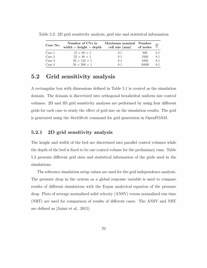
Table 5.2: 2D grid sensitivity analysis, grid size and statistical information
Case No.Number of CVs in
width × height × depthMaximum nominal
cell size (mm)Numberof nodes
∆Ldp
Case 1 15 × 60 × 1 8.1 900 8.1Case 2 22 × 88 × 1 8.1 1936 8.1Case 3 33 × 132 × 1 8.1 4356 8.1Case 4 50 × 200 × 1 8.1 10000 8.1
5.2 Grid sensitivity analysis
A rectangular box with dimensions defined in Table 5.1 is created as the simulation
domain. The domain is discretized into orthogonal hexahedral uniform size control
volumes. 2D and 3D grid sensitivity analyses are performed by using four different
grids for each case to study the effect of grid size on the simulation results. The grid
is generated using the blockMesh command for grid generation in OpenFOAM.
5.2.1 2D grid sensitivity analysis
The height and width of the bed are discretized into parallel control volumes while
the depth of the bed is fixed to be one control volume for the preliminary runs. Table
5.2 presents different grid sizes and statistical information of the grids used in the
simulations.
The reference simulation setup values are used for the grid independence analysis.
The pressure drop in the system as a global response variable is used to compare
results of different simulations with the Ergun analytical equation of the pressure
drop. Plots of average normalized solid velocity (ANSV) versus normalized run time
(NRT) are used for comparison of results of different cases. The ANSV and NRT
are defined as [Azimi et al., 2015]:
70
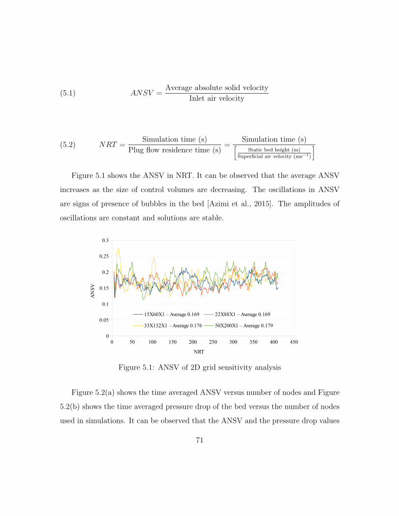
(5.1) ANSV =Average absolute solid velocity
Inlet air velocity
(5.2) NRT =Simulation time (s)
Plug flow residence time (s)=
Simulation time (s)[Static bed height (m)
Superficial air velocity (ms−1)
]
Figure 5.1 shows the ANSV in NRT. It can be observed that the average ANSV
increases as the size of control volumes are decreasing. The oscillations in ANSV
are signs of presence of bubbles in the bed [Azimi et al., 2015]. The amplitudes of
oscillations are constant and solutions are stable.
Figure 5.1: ANSV of 2D grid sensitivity analysis
Figure 5.2(a) shows the time averaged ANSV versus number of nodes and Figure
5.2(b) shows the time averaged pressure drop of the bed versus the number of nodes
used in simulations. It can be observed that the ANSV and the pressure drop values
71
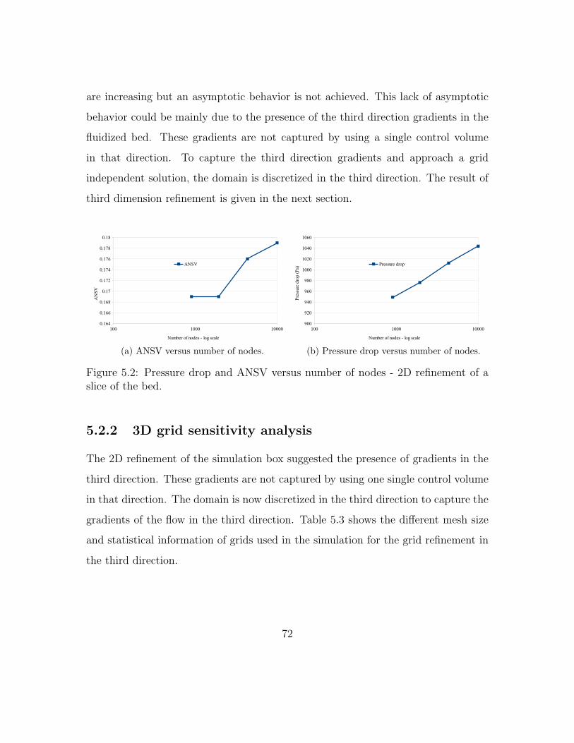
are increasing but an asymptotic behavior is not achieved. This lack of asymptotic
behavior could be mainly due to the presence of the third direction gradients in the
fluidized bed. These gradients are not captured by using a single control volume
in that direction. To capture the third direction gradients and approach a grid
independent solution, the domain is discretized in the third direction. The result of
third dimension refinement is given in the next section.
(a) ANSV versus number of nodes. (b) Pressure drop versus number of nodes.
Figure 5.2: Pressure drop and ANSV versus number of nodes - 2D refinement of aslice of the bed.
5.2.2 3D grid sensitivity analysis
The 2D refinement of the simulation box suggested the presence of gradients in the
third direction. These gradients are not captured by using one single control volume
in that direction. The domain is now discretized in the third direction to capture the
gradients of the flow in the third direction. Table 5.3 shows the different mesh size
and statistical information of grids used in the simulation for the grid refinement in
the third direction.
72
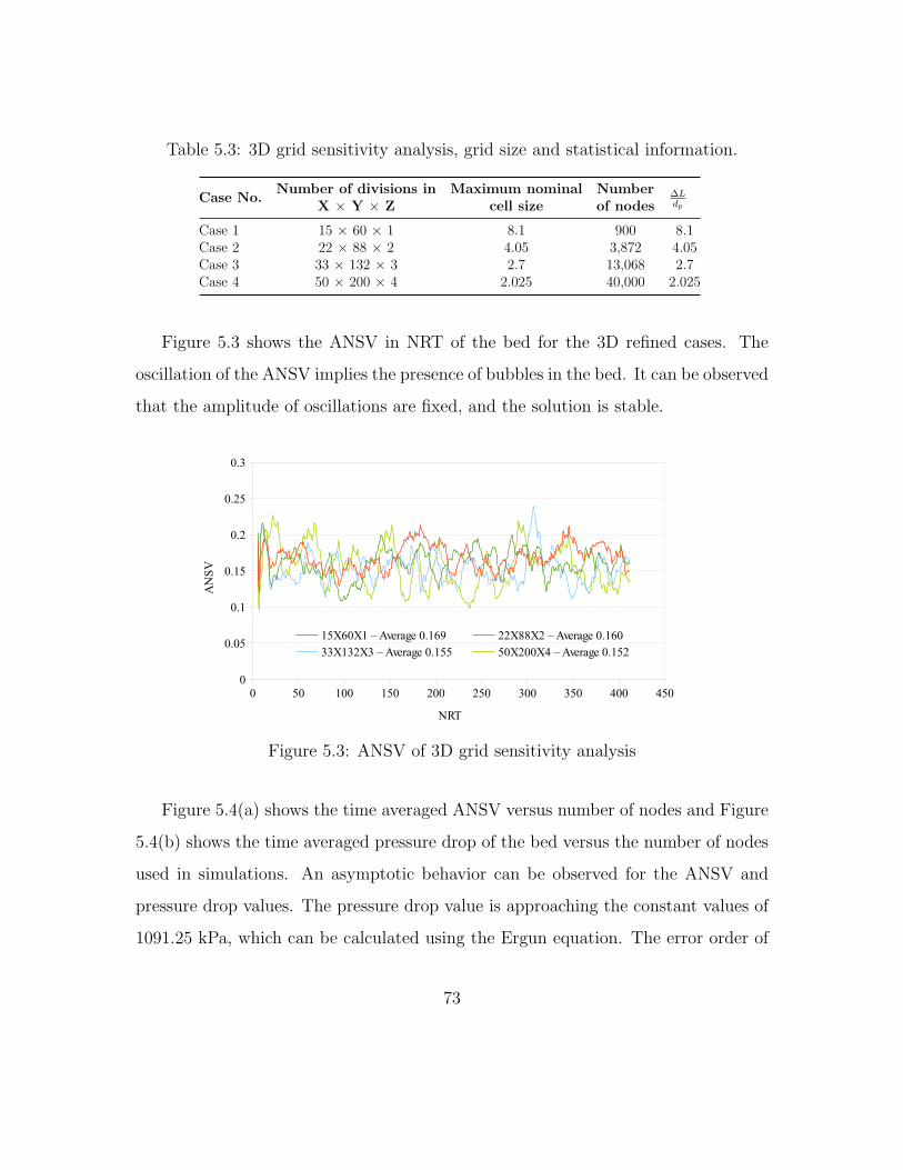
Table 5.3: 3D grid sensitivity analysis, grid size and statistical information.
Case No.Number of divisions in
X × Y × ZMaximum nominal
cell sizeNumberof nodes
∆Ldp
Case 1 15 × 60 × 1 8.1 900 8.1Case 2 22 × 88 × 2 4.05 3,872 4.05Case 3 33 × 132 × 3 2.7 13,068 2.7Case 4 50 × 200 × 4 2.025 40,000 2.025
Figure 5.3 shows the ANSV in NRT of the bed for the 3D refined cases. The
oscillation of the ANSV implies the presence of bubbles in the bed. It can be observed
that the amplitude of oscillations are fixed, and the solution is stable.
Figure 5.3: ANSV of 3D grid sensitivity analysis
Figure 5.4(a) shows the time averaged ANSV versus number of nodes and Figure
5.4(b) shows the time averaged pressure drop of the bed versus the number of nodes
used in simulations. An asymptotic behavior can be observed for the ANSV and
pressure drop values. The pressure drop value is approaching the constant values of
1091.25 kPa, which can be calculated using the Ergun equation. The error order of
73
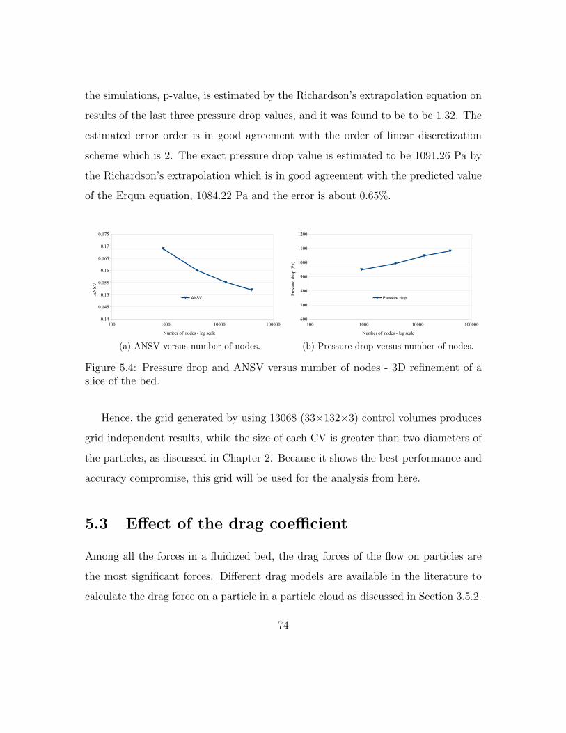
the simulations, p-value, is estimated by the Richardson’s extrapolation equation on
results of the last three pressure drop values, and it was found to be to be 1.32. The
estimated error order is in good agreement with the order of linear discretization
scheme which is 2. The exact pressure drop value is estimated to be 1091.26 Pa by
the Richardson’s extrapolation which is in good agreement with the predicted value
of the Erqun equation, 1084.22 Pa and the error is about 0.65%.
(a) ANSV versus number of nodes. (b) Pressure drop versus number of nodes.
Figure 5.4: Pressure drop and ANSV versus number of nodes - 3D refinement of aslice of the bed.
Hence, the grid generated by using 13068 (33×132×3) control volumes produces
grid independent results, while the size of each CV is greater than two diameters of
the particles, as discussed in Chapter 2. Because it shows the best performance and
accuracy compromise, this grid will be used for the analysis from here.
5.3 Effect of the drag coefficient
Among all the forces in a fluidized bed, the drag forces of the flow on particles are
the most significant forces. Different drag models are available in the literature to
calculate the drag force on a particle in a particle cloud as discussed in Section 3.5.2.
74

The available drag models in the CFDEM® coupling are Gidaspow [Gidaspow, 2012],
DiFelice [Di Felice, 1994], and Koch & Hill [Hill et al., 2001b] models.
The pressure drop along the bed is used as an integral quantity to show the effects
of drag models on the simulations results. Figure 5.5 shows computed instantaneous
pressure drop in the bed versus NRT. The Gidaspow drag model predicts lower
time averaged pressure drop in time compared to the two other drag models. Both
DiFelice and Koch & Hill drag models estimate the same time averaged pressure
drop values. All models converge to steady state and fluctuations in all cases are
a sign of presence of large bubbles or slugging in the bed, a poorly fluidized bed,
[Kunii and Levenspiel, 1969]. Kunii and Levenspiel [1969] predicted that the pressure
drop versus inlet velocity in a poorly fluidized bed might fluctuate up to 10% of the
mean value of the pressure drop. Figure 5.6 shows the diagram of pressure drop in a
poorly fluidized bed, where large bubbles are formed and slugging might happen in
the bed [Kunii and Levenspiel, 1969]. According to Equation 3.2 and Equation 3.1
the maximum and operating pressure drop of a bed with specifications of Table 6.3
are estimated to be 1130 Pa and 975 Pa, respectively.
75
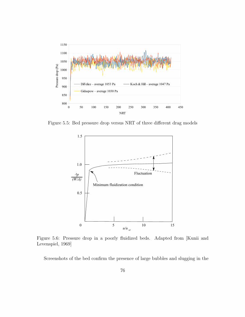
Figure 5.5: Bed pressure drop versus NRT of three different drag models
0 5 10 15
1.5
1.0
0.5
Minimum fluidization condition
u/u
Fluctuation�p
(W/A)
mf
Figure 5.6: Pressure drop in a poorly fluidized beds. Adapted from [Kunii andLevenspiel, 1969]
Screenshots of the bed confirm the presence of large bubbles and slugging in the
76
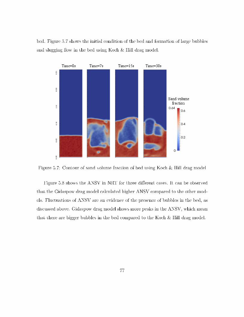
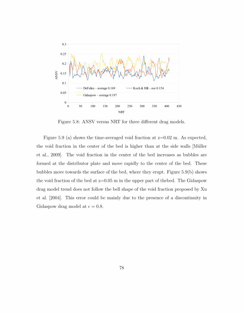
Figure 5.8: ANSV versus NRT for three different drag models.
Figure 5.9 (a) shows the time-averaged void fraction at z=0.02 m. As expected,
the void fraction in the center of the bed is higher than at the side walls [Muller
et al., 2009]. The void fraction in the center of the bed increases as bubbles are
formed at the distributor plate and move rapidly to the center of the bed. These
bubbles move towards the surface of the bed, where they erupt. Figure 5.9(b) shows
the void fraction of the bed at z=0.05 m in the upper part of thebed. The Gidaspow
drag model trend does not follow the bell shape of the void fraction proposed by Xu
et al. [2004]. This error could be mainly due to the presence of a discontinuity in
Gidaspow drag model at ε = 0.8.
78

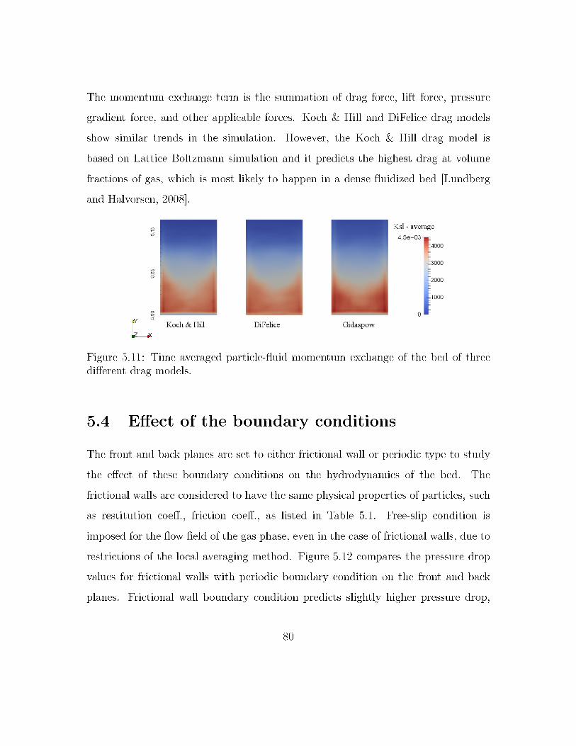

which could be caused by dissipation of particles’ kinetic energy and formation of
dense zones in the bed.
Figure 5.12: Bed pressure drop versus NRT for frictional wall and periodic boundaryconditions.
Figure 5.13 presents the ANSV versus NRT comparison for these cases. It can
be observed that the time averaged ANSV for the frictional wall condition is 52%
less than the periodic boundary condition. The different calculated values of ANSV
confirms the idea of dissipation of particles’ kinetic energy when colliding with the
walls.
81
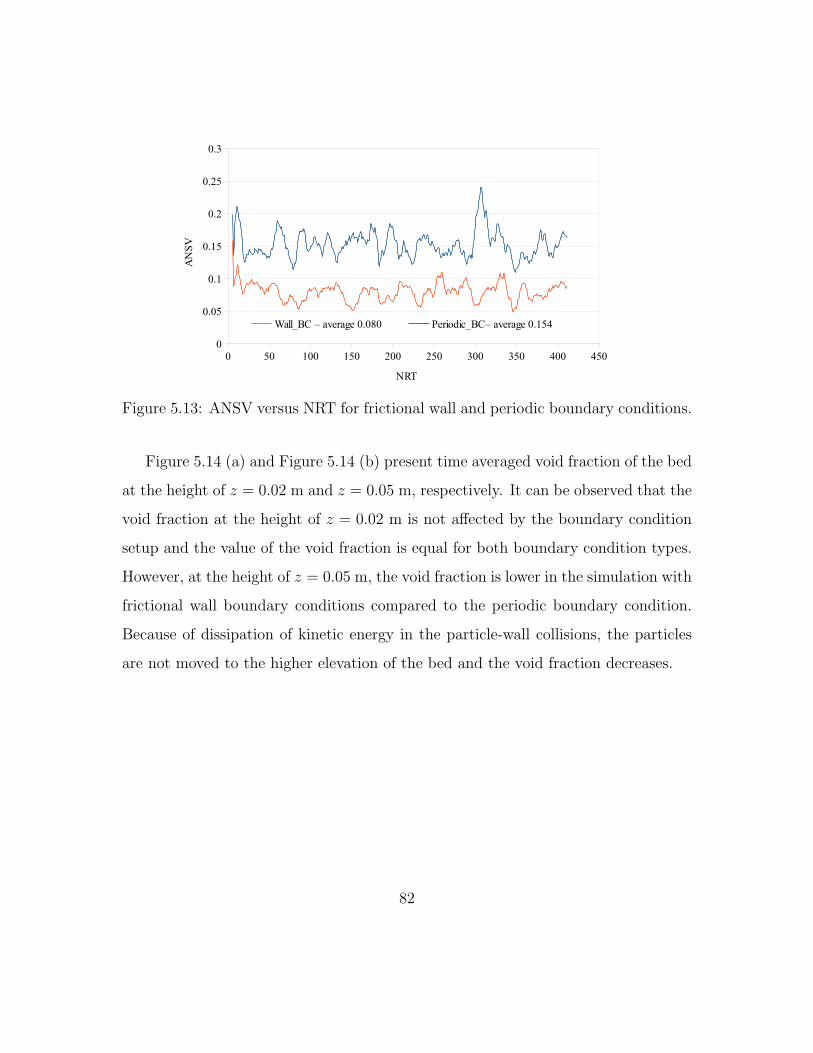
Figure 5.13: ANSV versus NRT for frictional wall and periodic boundary conditions.
Figure 5.14 (a) and Figure 5.14 (b) present time averaged void fraction of the bed
at the height of z = 0.02 m and z = 0.05 m, respectively. It can be observed that the
void fraction at the height of z = 0.02 m is not affected by the boundary condition
setup and the value of the void fraction is equal for both boundary condition types.
However, at the height of z = 0.05 m, the void fraction is lower in the simulation with
frictional wall boundary conditions compared to the periodic boundary condition.
Because of dissipation of kinetic energy in the particle-wall collisions, the particles
are not moved to the higher elevation of the bed and the void fraction decreases.
82

(a) At z=0.02 m (b) At z=0.05 m
Figure 5.14: Time averaged void fraction of the bed of frictional wall and periodicboundary conditions at z = 0.02 m (a) and z=0.05 m (b).
5.5 Model A and Model B
The treatment of the momentum exchange term, as discussed in Section 3.5.2, plays
a significant role in the result of simulations of gas-solid flows. There has been
extensive research on the effect of the treatment of momentum exchange term on
the flow field in fluidization process. The objective of the current analysis is to
demonstrate differences in the results of simulations using the momentum exchange
term models. The pressure drop of the bed in time and ANSV versus NRT are
considered to study the effect of the momentum exchange term on the results of the
simulations.
Table 5.4 presents the treatment of momentum exchange term and forces which
are included in each case.
83
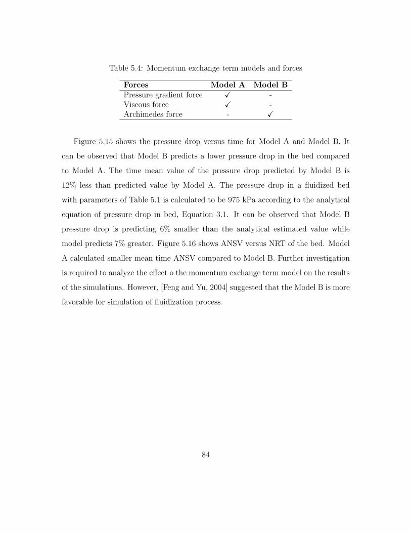
Table 5.4: Momentum exchange term models and forces
Forces Model A Model BPressure gradient force X -Viscous force X -Archimedes force - X
Figure 5.15 shows the pressure drop versus time for Model A and Model B. It
can be observed that Model B predicts a lower pressure drop in the bed compared
to Model A. The time mean value of the pressure drop predicted by Model B is
12% less than predicted value by Model A. The pressure drop in a fluidized bed
with parameters of Table 5.1 is calculated to be 975 kPa according to the analytical
equation of pressure drop in bed, Equation 3.1. It can be observed that Model B
pressure drop is predicting 6% smaller than the analytical estimated value while
model predicts 7% greater. Figure 5.16 shows ANSV versus NRT of the bed. Model
A calculated smaller mean time ANSV compared to Model B. Further investigation
is required to analyze the effect o the momentum exchange term model on the results
of the simulations. However, [Feng and Yu, 2004] suggested that the Model B is more
favorable for simulation of fluidization process.
84

Figure 5.15: Bed pressure drop using Model A and Model B for momentum exchangeterm.
Figure 5.16: ANSV versus NRT, Model A and Model B for momentum exchangeterm.
85
Chapter 6
Simulation of segregation of
particles in fluidized bed
The Discrete Element Method (DEM) is used to study the segregation of particles
in a fluidized bed. Following results of the fluidization process in Chapter 5, the
simulation settings, such as mesh size and numerical schemes, are set. The Lacey
mixing index is used to quantify the quality of the mixture and provide a statistical
picture of it. The affecting parameters on the mixing index are studied to analyze
the sensitivity of the mixing index and provide an accurate picture of the mixture.
The segregation process is analyzed in a bed formed by a binary mixture of
particles with a high density ratio (2.5) at the first step to analyze the effect of
boundary conditions and momentum exchange model. The effect of superficial inlet
velocity on the final quality of the mixture and rate of segregation of particles is
explained.
Later, the density ratio of the mixture components is decreased to 1.33 in order to
increase the sensitivity of the segregation process and analyze the effect of different
86
parameters on the quality of the mixture. The effect of carrier phase properties and
the aspect ratio of the bed on the final quality of mixture and rate of segregation is
analyzed.
6.1 Lacey mixing index
The Lacey mixing index [Lacey, 1954], as described in Section 3.6.3, can be used to
quantify the quality of the mixture. The Lacey mixing index compares the achieved
mixing to the possible mixture, which is based on statistical analysis. Based on this
statistical approach, the following parameters should be considered in the calcula-
tion of the mixing index: box width and the sample size. Both are investigated to
determine their optimal values. The value of the mixing index is substituted by the
average of the ten neighboring points in time to remove the noise from the plots of
the Lacey mixing index.
6.1.1 Box width
The DEM method uses an adjustable sample size and a proper sample size needs to
be determined which represents an accurate statistical picture of the mixture. Rect-
angular boxes are used to discretize the domain and obtain samples of the mixture.
Once the width of the boxes are fixed, the height of the boxes are changed so that
the total number of particles in each sample is the same and the scale of scrutiny
is fixed. A Matlab code was developed for this purpose, which can be reached at
Appendix B.
Table 6.1 shows for all the test cases the number of particles in each sample box
and the number of divisions in the width of the bed to measure the mixing index.
87
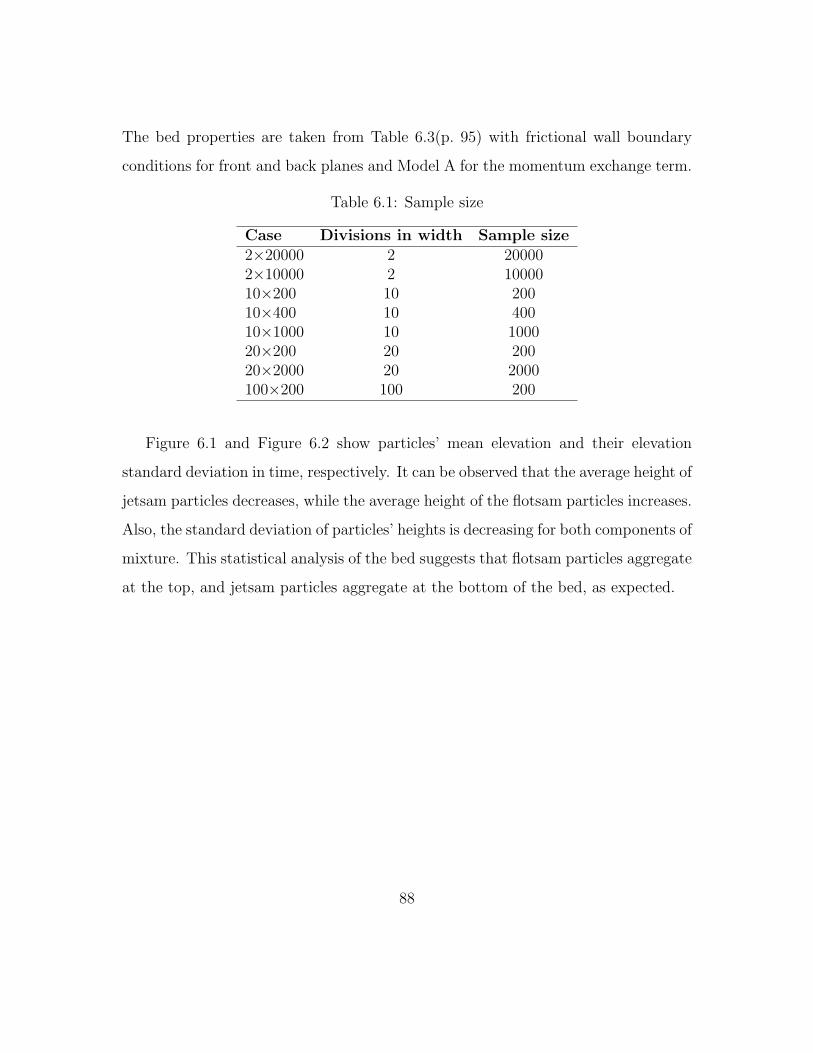
The bed properties are taken from Table 6.3(p. 95) with frictional wall boundary
conditions for front and back planes and Model A for the momentum exchange term.
Table 6.1: Sample size
Case Divisions in width Sample size2×20000 2 200002×10000 2 1000010×200 10 20010×400 10 40010×1000 10 100020×200 20 20020×2000 20 2000100×200 100 200
Figure 6.1 and Figure 6.2 show particles’ mean elevation and their elevation
standard deviation in time, respectively. It can be observed that the average height of
jetsam particles decreases, while the average height of the flotsam particles increases.
Also, the standard deviation of particles’ heights is decreasing for both components of
mixture. This statistical analysis of the bed suggests that flotsam particles aggregate
at the top, and jetsam particles aggregate at the bottom of the bed, as expected.
88
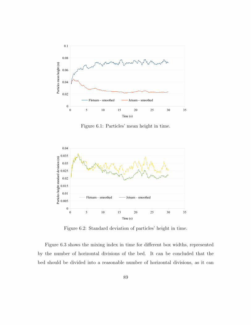
Figure 6.1: Particles’ mean height in time.
Figure 6.2: Standard deviation of particles’ height in time.
Figure 6.3 shows the mixing index in time for different box widths, represented
by the number of horizontal divisions of the bed. It can be concluded that the
bed should be divided into a reasonable number of horizontal divisions, as it can
89
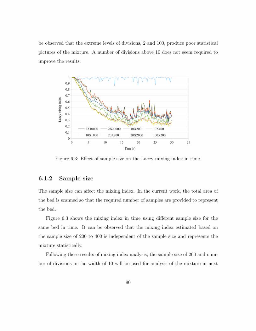
be observed that the extreme levels of divisions, 2 and 100, produce poor statistical
pictures of the mixture. A number of divisions above 10 does not seem required to
improve the results.
Figure 6.3: Effect of sample size on the Lacey mixing index in time.
6.1.2 Sample size
The sample size can affect the mixing index. In the current work, the total area of
the bed is scanned so that the required number of samples are provided to represent
the bed.
Figure 6.3 shows the mixing index in time using different sample size for the
same bed in time. It can be observed that the mixing index estimated based on
the sample size of 200 to 400 is independent of the sample size and represents the
mixture statistically.
Following these results of mixing index analysis, the sample size of 200 and num-
ber of divisions in the width of 10 will be used for analysis of the mixture in next
90

sections.
6.2 Validation
Feng and Yu [2004] analyzed segregation of a binary mixture of particles in a fluidized
bed by performing numerical simulations and experiments. A binary mixture of
particles with the same density and different diameters was fluidized for enough time
to be segregated. They compared results of the numerical simulations to experiments.
A series of simulations with same conditions as their work is considered to validate the
CFDEM® coupling software. A rectangular box with the same dimensions of their
work is used as the simulation domain which is discretized into orthogonal hexahedral
control volumes, as described in Section 5.2. Description of the simulation settings
can be found in Table 5.1. Table 6.2 presents the solid phase properties.
Table 6.2: Parameters used for the validation case adapted from Feng and Yu [2004]
Description Particle Value CommentParticle density(kg m−3)
Flotsam 2500 SandJetsam 2500 Sand
Particle diameter(mm)
Flotsam 1 ConstantJetsam 2 Constant
Numberof particles
Flotsam 22,223 50% mass fractionJetsam 2,777 50% mass fraction
For a fluidized bed formed from particles described in Table 6.2, the maximum
pressure drop of the bed is calculated to be 1083 Pa using Equations 3.1. Figure
6.4 presents the variation of pressure drop in time using Model A for momentum
exchange model, when the superficial gas velocity is 1.2 m s−1. The mean value of
the numerical pressure drop in the study by Feng and Yu [2004] using Model A is
91
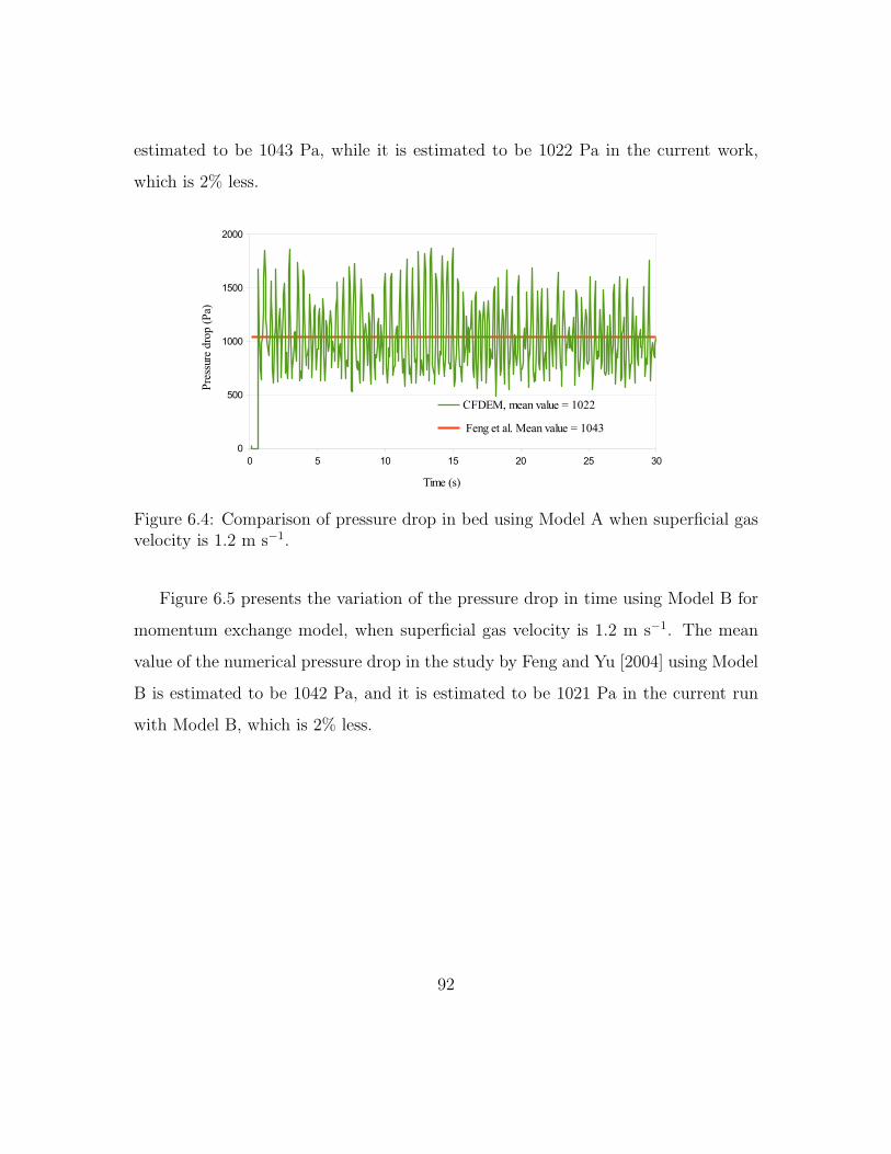
estimated to be 1043 Pa, while it is estimated to be 1022 Pa in the current work,
which is 2% less.
Figure 6.4: Comparison of pressure drop in bed using Model A when superficial gasvelocity is 1.2 m s−1.
Figure 6.5 presents the variation of the pressure drop in time using Model B for
momentum exchange model, when superficial gas velocity is 1.2 m s−1. The mean
value of the numerical pressure drop in the study by Feng and Yu [2004] using Model
B is estimated to be 1042 Pa, and it is estimated to be 1021 Pa in the current run
with Model B, which is 2% less.
92
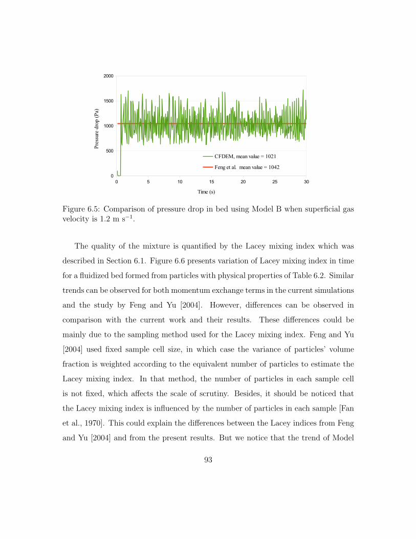
Figure 6.5: Comparison of pressure drop in bed using Model B when superficial gasvelocity is 1.2 m s−1.
The quality of the mixture is quantified by the Lacey mixing index which was
described in Section 6.1. Figure 6.6 presents variation of Lacey mixing index in time
for a fluidized bed formed from particles with physical properties of Table 6.2. Similar
trends can be observed for both momentum exchange terms in the current simulations
and the study by Feng and Yu [2004]. However, differences can be observed in
comparison with the current work and their results. These differences could be
mainly due to the sampling method used for the Lacey mixing index. Feng and Yu
[2004] used fixed sample cell size, in which case the variance of particles’ volume
fraction is weighted according to the equivalent number of particles to estimate the
Lacey mixing index. In that method, the number of particles in each sample cell
is not fixed, which affects the scale of scrutiny. Besides, it should be noticed that
the Lacey mixing index is influenced by the number of particles in each sample [Fan
et al., 1970]. This could explain the differences between the Lacey indices from Feng
and Yu [2004] and from the present results. But we notice that the trend of Model
93
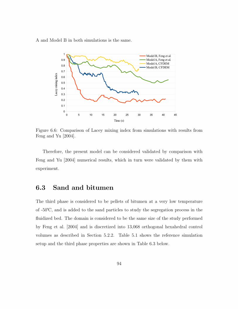
A and Model B in both simulations is the same.
Figure 6.6: Comparison of Lacey mixing index from simulations with results fromFeng and Yu [2004].
Therefore, the present model can be considered validated by comparison with
Feng and Yu [2004] numerical results, which in turn were validated by them with
experiment.
6.3 Sand and bitumen
The third phase is considered to be pellets of bitumen at a very low temperature
of -50℃, and is added to the sand particles to study the segregation process in the
fluidized bed. The domain is considered to be the same size of the study performed
by Feng et al. [2004] and is discretized into 13,068 orthogonal hexahedral control
volumes as described in Section 5.2.2. Table 5.1 shows the reference simulation
setup and the third phase properties are shown in Table 6.3 below.
94

Table 6.3: Reference simulation settings
Description Particle Value CommentParticle density(kg m−3)
Flotsam 1000 Bitumen at -50℃Jetsam 2500 Sand at -50℃
Particle diameter(mm)
Flotsam 1 ConstantJetsam 1 Constant
Numberof particles
Flotsam 20,000 50% volume fractionJetsam 20,000 50% volume fraction
The packed bed is formed by inserting particles at random positions in the bed
without overlapping, when there is no gas injected to the inlet at the presence of the
gravity field for 0.5 s. Particles are settled and a packed bed of random mixture is
formed. Then, the gas is uniformly injected at the inlet and particles are fluidized.
The pressure drop of the bed is considered a charectiristic quantity to compare with
Equation 3.1, the analytical solution of pressure drop for validation of the results.
Averaged normalized solid velocity (ANSV) versus normalized run time (NRT) is
plotted to study the hydrodynamics of the bed.
Lacey mixing index is used as a tool to quantify the quality of mixture and to
compare the simulation results with published data.
6.3.1 Effect of the boundary conditions and momentum ex-
change model
Comparison with 3D case
Following results of simulations of fluidization process in Section 5.4 the front and
back planes condition can affect the hydrodynamics of the fluidized bed. Here, the
effect of boundary conditions applied to these planes on the results of segregation
process simulation is studied carefully to increase the accuracy of the results. Peri-
95

odic, frictional wall, and reflective walls are considered for this purpose, and results
of the narrow channel case are compared with the simulation of a bed with a square
(0.065×0.065 m) cross-section, referred to as the 3D case. The total number of par-
ticles is changed to 321,000 particles to keep the height of the bed the same as the
narrow channel case. The bed is discretized into 143,748 (33×33×132) orthogonal
hexahedral control volumes. Models A and B of momentum exchange are considered
separately. Table 6.4 presents front and back planes setup used in the simulations.
Table 6.4: Different boundary conditions used in simulation models.
Description Phase Value
PeriodicGas phase Periodic boundary conditionParticles Periodic boundary condition
Frictional wallGas phase Slip wallParticles Frictional wall, e=0.9
Reflective wallGas phase Slip wallParticles Reflective wall
3D caseGas phase Slip wallParticles Frictional wall, e=0.9
96
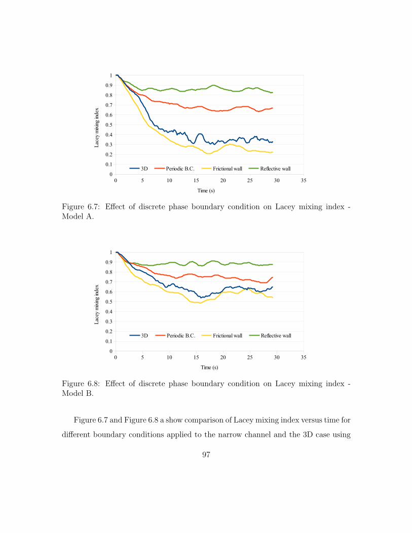
Figure 6.7: Effect of discrete phase boundary condition on Lacey mixing index -Model A.
Figure 6.8: Effect of discrete phase boundary condition on Lacey mixing index -Model B.
Figure 6.7 and Figure 6.8 a show comparison of Lacey mixing index versus time for
different boundary conditions applied to the narrow channel and the 3D case using
97
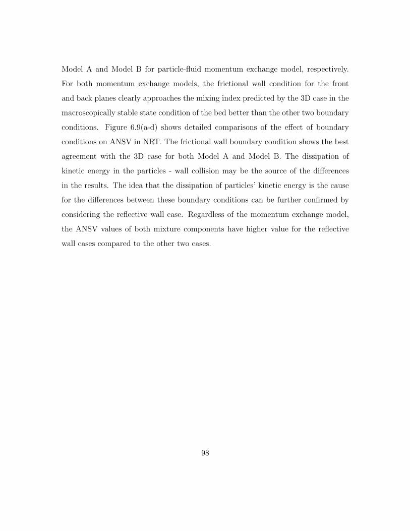
Model A and Model B for particle-fluid momentum exchange model, respectively.
For both momentum exchange models, the frictional wall condition for the front
and back planes clearly approaches the mixing index predicted by the 3D case in the
macroscopically stable state condition of the bed better than the other two boundary
conditions. Figure 6.9(a-d) shows detailed comparisons of the effect of boundary
conditions on ANSV in NRT. The frictional wall boundary condition shows the best
agreement with the 3D case for both Model A and Model B. The dissipation of
kinetic energy in the particles - wall collision may be the source of the differences
in the results. The idea that the dissipation of particles’ kinetic energy is the cause
for the differences between these boundary conditions can be further confirmed by
considering the reflective wall case. Regardless of the momentum exchange model,
the ANSV values of both mixture components have higher value for the reflective
wall cases compared to the other two cases.
98
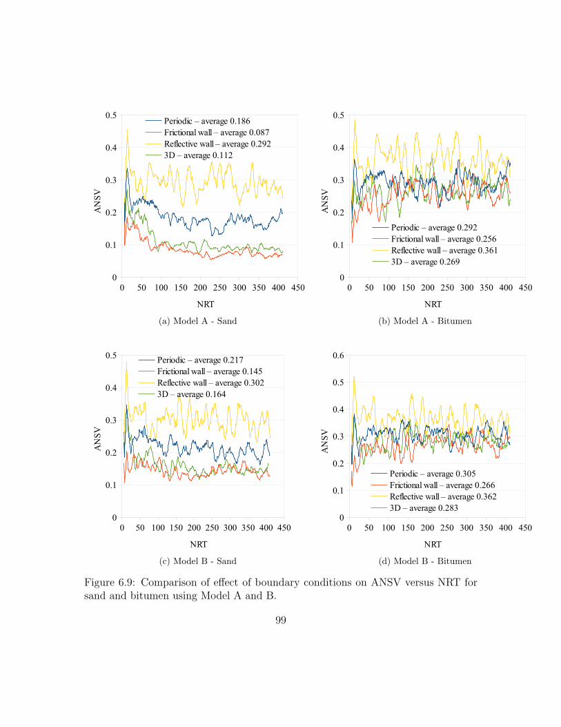
(a) Model A - Sand (b) Model A - Bitumen
(c) Model B - Sand (d) Model B - Bitumen
Figure 6.9: Comparison of effect of boundary conditions on ANSV versus NRT forsand and bitumen using Model A and B.
99
Initial condition of the bed
The effect of the initial condition of the bed on the segregation process is examined by
considering two different scenarios: an initially randomly mixed bed and an initially
inversely segregated bed. The formation of the randomly mixed bed was discussed
in Section 6.3. The inversely segregated bed is formed by inserting particles in two
separate boxes at different elevations. The flotsam particles are inserted in the lower
half of the bed height, and jetsam particles are inserted in the top portion of the
bed. Particles are settled in the presence of gravity when there is no gas injected at
the inlet for 0.5 s.
Figure 6.10 shows the Lacey mixing index in time using periodic boundary con-
dition for the front and back planes. It can be observed that at the macroscopically
stable state of the bed, the Lacey mixing index is independent of the initial condition
of the bed for both momentum exchange models. In an initially segregated packed
bed with periodic boundary conditions for front and back planes, particles are lifted
and moved upward when the gas is injected to the inlet, then mixing starts after a
very short period with Model A or after a significant period with the Model B type
of momentum exchange, as explained next.
100
Figure 6.10: Effect of initial condition on Lacey mixing index - Periodic boundarycondition.
Figure 6.11 and Figure 6.12 show snapshots of the bed at different time steps
using periodic boundary conditions for the front and back planes, and Model A and
Model B. For the initially inverse segregated packed bed, particles are lifted and
moved to the outlet, where they block the outlet for 18 seconds, if Model A is used
for momentum exchange and periodic boundary condition is set for front and back
planes. Same results can be observed when Model B is used for the momentum
exchange term in an inverse segregated packed bed. However, in this case, the
particle cloud at the outlet collapses in less than 2 seconds.
101


Figure 6.13 again shows the Lacey mixing index in time, but now using frictional
wall boundary condition for the front and back planes. It can be observed that at
the macroscopically stable state of the bed, the Lacey mixing index is independent
of the initial condition for both boundary conditions (frictional, as well as periodic)
and both momentum exchange models. However, a big difference can be observed
between the predicted values by Model A and Model B in the case of the frictional
boundaries. As it was described in Section 3.5.2, pointwise pressure drop values are
needed to calculate the particle - fluid interaction forces. However, by using the local
average method pointwise pressure values are not available and only mean values are
calculated. This results in differences between the results of Model A and B [Feng
and Yu, 2004]. Feng and Yu [2004] verified results of the simulation of a fluidized
bed using Model A and Model B for momentum conservation equation set against
experiments quantitatively and qualitatively and suggested that results of Model B
are more favorable.
Figure 6.13: Effect of initial condition on Lacey mixing index - frictional wall bound-ary condition.
103
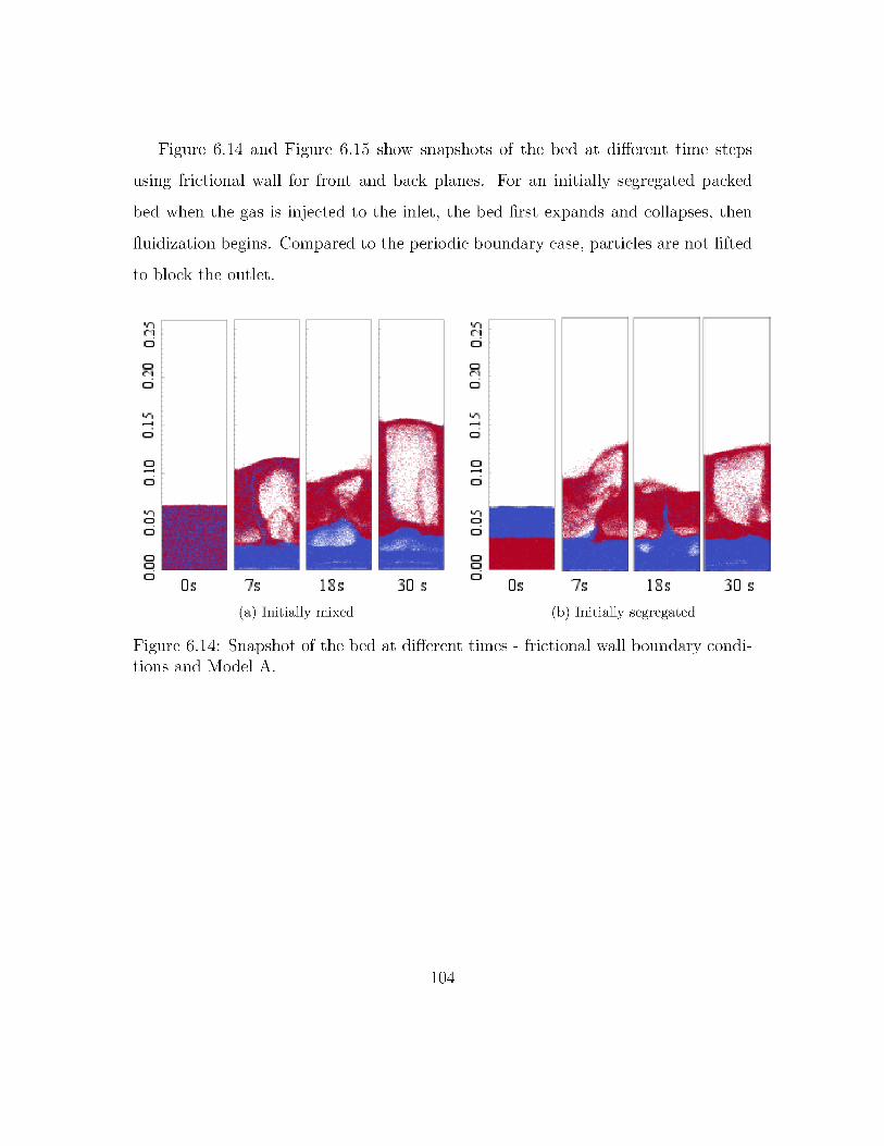

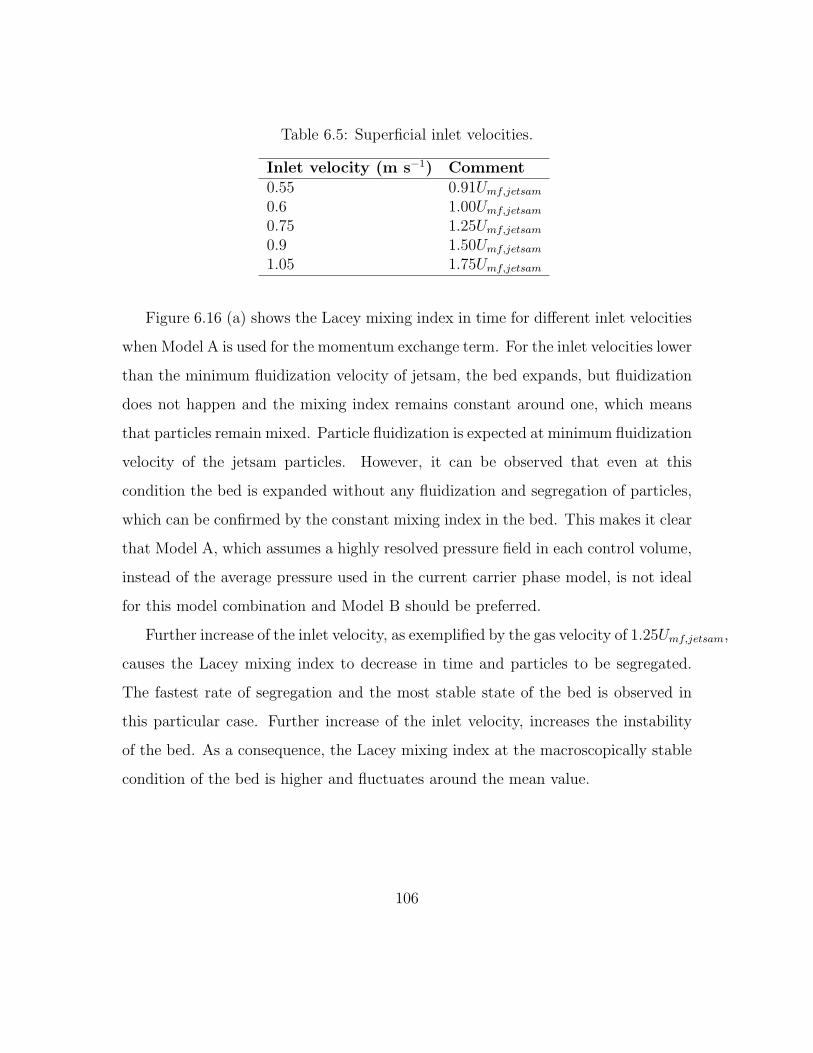
Table 6.5: Superficial inlet velocities.
Inlet velocity (m s−1) Comment0.55 0.91Umf,jetsam
0.6 1.00Umf,jetsam
0.75 1.25Umf,jetsam
0.9 1.50Umf,jetsam
1.05 1.75Umf,jetsam
Figure 6.16 (a) shows the Lacey mixing index in time for different inlet velocities
when Model A is used for the momentum exchange term. For the inlet velocities lower
than the minimum fluidization velocity of jetsam, the bed expands, but fluidization
does not happen and the mixing index remains constant around one, which means
that particles remain mixed. Particle fluidization is expected at minimum fluidization
velocity of the jetsam particles. However, it can be observed that even at this
condition the bed is expanded without any fluidization and segregation of particles,
which can be confirmed by the constant mixing index in the bed. This makes it clear
that Model A, which assumes a highly resolved pressure field in each control volume,
instead of the average pressure used in the current carrier phase model, is not ideal
for this model combination and Model B should be preferred.
Further increase of the inlet velocity, as exemplified by the gas velocity of 1.25Umf,jetsam,
causes the Lacey mixing index to decrease in time and particles to be segregated.
The fastest rate of segregation and the most stable state of the bed is observed in
this particular case. Further increase of the inlet velocity, increases the instability
of the bed. As a consequence, the Lacey mixing index at the macroscopically stable
condition of the bed is higher and fluctuates around the mean value.
106
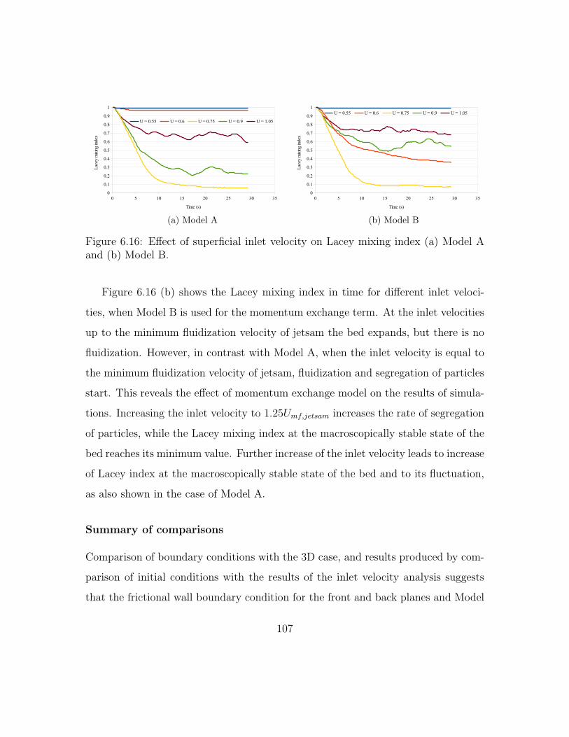
(a) Model A (b) Model B
Figure 6.16: Effect of superficial inlet velocity on Lacey mixing index (a) Model Aand (b) Model B.
Figure 6.16 (b) shows the Lacey mixing index in time for different inlet veloci-
ties, when Model B is used for the momentum exchange term. At the inlet velocities
up to the minimum fluidization velocity of jetsam the bed expands, but there is no
fluidization. However, in contrast with Model A, when the inlet velocity is equal to
the minimum fluidization velocity of jetsam, fluidization and segregation of particles
start. This reveals the effect of momentum exchange model on the results of simula-
tions. Increasing the inlet velocity to 1.25Umf,jetsam increases the rate of segregation
of particles, while the Lacey mixing index at the macroscopically stable state of the
bed reaches its minimum value. Further increase of the inlet velocity leads to increase
of Lacey index at the macroscopically stable state of the bed and to its fluctuation,
as also shown in the case of Model A.
Summary of comparisons
Comparison of boundary conditions with the 3D case, and results produced by com-
parison of initial conditions with the results of the inlet velocity analysis suggests
that the frictional wall boundary condition for the front and back planes and Model
107
B for the momentum exchange term produce better qualitative and quantitative re-
sults. Model B can be used to study the segregation process in a bed formed from
clay and bitumen pellets.
Results of inlet velocity comparison show that when the gas velocity is set to 1.25
times the minimum fluidization velocity of jetsam, the rate of segregation of partici-
ples is the highest, and the mixing index has a lower value at the macroscopically
stable state of the bed.
6.4 Clay and bitumen
In addition to the inlet velocity, the other factor which has a significant effect on the
segregation process is the density ratio of the mixture components. A smaller density
ratio is considered to increase the sensitivity of the problem. The density ratio is
changed from 2.5 in the previous section to 1.33. Two different types of particles
are considered. It is assumed that the jetsam particles are made of a mixture of
bitumen and sand with a density of 1600 kg m−3 and the flotsam particles are pellets
of clay with the density of 1200 kg m−3. Following results of Section 6.3, the Model
B is used for the momentum exchange term, the frictional wall boundary condition
is used on the front and back planes, and the superficial inlet velocity is set to be
1.25Umf,jetsam.
The effects of the carrier phase properties and of the bed aspect ratio on the
mixture quality are studied in the following sections.
108
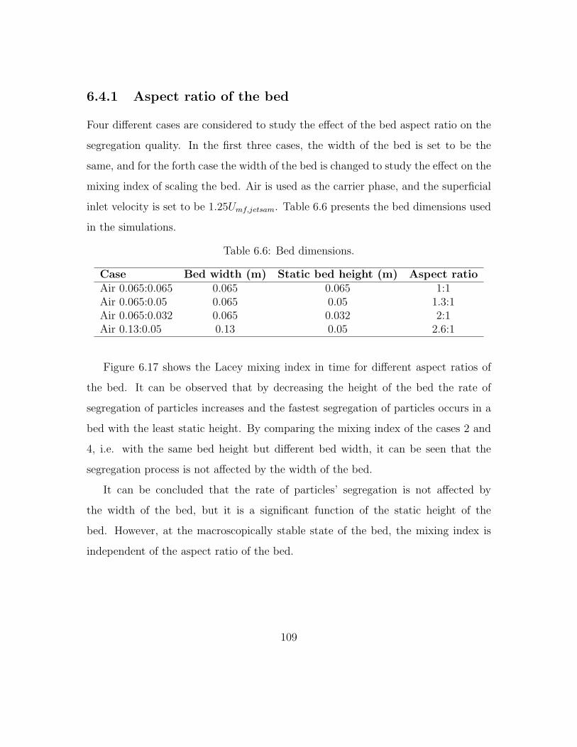
6.4.1 Aspect ratio of the bed
Four different cases are considered to study the effect of the bed aspect ratio on the
segregation quality. In the first three cases, the width of the bed is set to be the
same, and for the forth case the width of the bed is changed to study the effect on the
mixing index of scaling the bed. Air is used as the carrier phase, and the superficial
inlet velocity is set to be 1.25Umf,jetsam. Table 6.6 presents the bed dimensions used
in the simulations.
Table 6.6: Bed dimensions.
Case Bed width (m) Static bed height (m) Aspect ratioAir 0.065:0.065 0.065 0.065 1:1Air 0.065:0.05 0.065 0.05 1.3:1Air 0.065:0.032 0.065 0.032 2:1Air 0.13:0.05 0.13 0.05 2.6:1
Figure 6.17 shows the Lacey mixing index in time for different aspect ratios of
the bed. It can be observed that by decreasing the height of the bed the rate of
segregation of particles increases and the fastest segregation of particles occurs in a
bed with the least static height. By comparing the mixing index of the cases 2 and
4, i.e. with the same bed height but different bed width, it can be seen that the
segregation process is not affected by the width of the bed.
It can be concluded that the rate of particles’ segregation is not affected by
the width of the bed, but it is a significant function of the static height of the
bed. However, at the macroscopically stable state of the bed, the mixing index is
independent of the aspect ratio of the bed.
109
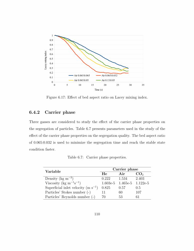
Figure 6.17: Effect of bed aspect ratio on Lacey mixing index.
6.4.2 Carrier phase
Three gasses are considered to study the effect of the carrier phase properties on
the segregation of particles. Table 6.7 presents parameters used in the study of the
effect of the carrier phase properties on the segregation quality. The bed aspect ratio
of 0.065:0.032 is used to minimize the segregation time and reach the stable state
condition faster.
Table 6.7: Carrier phase properties.
VariableCarrier phase
He Air CO2
Density (kg m−3) 0.222 1.534 2.403Viscosity (kg m−1s−1) 1.603e-5 1.465e-5 1.122e-5Superficial inlet velocity (m s−1) 0.825 0.57 0.5Particles’ Stokes number (-) 11 60 107Particles’ Reynolds number (-) 70 53 61
110
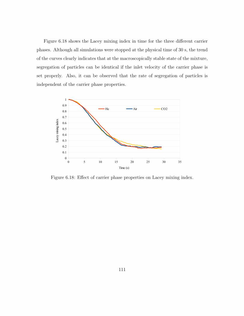
Figure 6.18 shows the Lacey mixing index in time for the three different carrier
phases. Although all simulations were stopped at the physical time of 30 s, the trend
of the curves clearly indicates that at the macroscopically stable state of the mixture,
segregation of particles can be identical if the inlet velocity of the carrier phase is
set properly. Also, it can be observed that the rate of segregation of particles is
independent of the carrier phase properties.
Figure 6.18: Effect of carrier phase properties on Lacey mixing index.
111
Chapter 7
Conclusion and future work
7.1 Conclusion
The open source CFDEM® coupling was used as the software to develop a model for
the process of fluidization and segregation of particles. The Average Normalized Solid
Velocity (ANSV) and the pressure drop versus Normalized Run Time (NRT) were
used to verify and validate the model. Results of simulations suggest the following
conclusions an recommendations for model setup.
• A slice of the bed could be used to represent a full bed, if the slice grid is
discretized in the depth to capture the gradients of the flow.
• The frictional wall boundary condition for the front and back planes of the
bed slice predicts more accurate results compared to the periodic boundary
condition, as it represents better the full size bed.
• The cell size of 2.7 times the particle diameter was found to be suitable to
predict the correct pressure drop and grid independent solution.
112
• The set of Model A momentum conservation equations and also the set of
Model B momentum conservation equations predict the same pressure drop
values. However, comparison of the results of the Lacey mixing index for both
models and also comparison of the results of different inlet velocities suggest
that Model B is more favorable to be used to model the fluidized bed, as
mentioned by Feng and Yu [2004].
• Koch & Hill, DeFelice and Gidaspow drag models were used to study the effect
of drag model on simulations results. The Gidaspow drag model predicted the
least pressure drop in the bed compared to DeFelice, and Koch & Hill drag
models. The Gidaspow drag model did not follow the bell shape of the void
fraction profile proposed by Xu et al. [2004]. The Koch & Hill drag model
predicted higher drag at volume fractions compared to DiFelice, which is most
likely to happen in a dense fluidized bed.
• The solution of the numerical model, after reaching the macroscopically stable
state of the bed, should be independent of the initial conditions, if the boundary
conditions and the momentum conservation equations are set properly.
The developed numerical model in the CFDEM® coupling was used to study the
effect of the operating conditions of the bed on the segregation process. Particles
of the same size and density ratios of 2.5 and 1.33 were considered to examine the
segregation process. The ANSV versus NRT and Lacey mixing index versus time
were considered to analyze the results, and quantify the quality of the mixture.
Results of simulations suggest the following conclusions and recommendations.
• There is an optimum superficial inlet velocity for the segregation of particles in
a fluidized bed as it was suggested by Feng and Yu [2007]. The inlet velocity
113
of 1.25Umf,jetsam was found to segregate particles with the highest rate among
the tested velocities. This means that the lowest Lacey mixing index at the
macroscopically stable state of the bed was observed at this inlet velocity. Also
the fastest rate of segregation was found at this same inlet velocity.
• The static height of the bed is inversely correlated with the rate of segregation of
particles. However, the macroscopically stable state of the bed is independent
of the static height of the bed.
• The rate of segregation of particles and the final state of the bed are indepen-
dent of the width of the bed.
• The carrier phase thermo-physical properties do not affect the macroscopically
stable state of the bed.
7.2 Future work
The current analysis of the segregation process considers a batch of the mixture.
However, in the industrial applications of the fluidized bed, the process is mostly a
continuous process. The continuous process of segregation of particles can be studied
using Eulerian - Lagrangian approach by the CFDEM® coupling software.
The jetsam and flotsam are considered to be the same size. However, the size
ratio is one of the dominant factors in segregation of particles. It is necessary to
study segregation of particles considering the size ratio of the particles.
In the current work the particles’ size is considered to be uniform, and particle
size distribution is neglected. However, particles’ sizes are mostly distributed about
a mean value. It is necessary to study the segregation of particles considering the
114

size distribution. The Lagrangian approach allows to introduce the size distribution
without increasing the complexity of the problem.
The current work assumes particles to be spherical and the shape factor of parti-
cles is neglected. However, the shape factor can affect the initial packing of the bed
and the drag forces on the particles. It is necessary to study the effect of particles
shape factor on the fluidization and segregation processes.
Due to limitations on the available computational power, the size of the bed
was considered to be relatively small in the current work. It is necessary to study
the scaling process on the fluidization and segregation processes and identify sig-
nificant factors in the scaling procedure. Discrete Particle Method (DPM) can be
implemented to analyze the fluidization and segregation processes in industrial size
fluidized beds by considering parcels of particles.
Cooling of particles was one of the objectives of segregation of particles in a
fluidized bed in the proposed mechanical separation of bitumen and clay method.
However in the current work, the heat transfer was not considered, and it is necessary
to consider the heat transfer in the fluidization and segregation processes as one of
the objectives of the proposed method.
115

Bibliography
Government Alberta. Alberta energy: Facts and statistics, 2016. URL http://www.
energy.alberta.ca/oilsands/791.asp.
T Bo Anderson and Roy Jackson. Fluid mechanical description of fluidized beds.
Equations of motion. Industrial & Engineering Chemistry Fundamentals, 6(4):
527–539, 1967.
Ebrahim Azimi. Simulation and performance characterization of air dense medium
fluidized bed for coal beneficiation. PhD thesis, University of Alberta, 2014.
Ebrahim Azimi, Shayan Karimipour, Petr Nikrityuk, Jozef Szymanski, and Rajender
Gupta. Numerical simulation of 3-phase fluidized bed particle segregation. Fuel,
150:347–359, 2015.
Ralph A Bagnold. Experiments on a gravity-free dispersion of large solid spheres in
a Newtonian fluid under shear. In Proceedings of the Royal Society of London A:
Mathematical, Physical and Engineering Sciences, volume 225, pages 49–63. The
Royal Society, 1954.
HT Bi and JR Grace. Flow regime diagrams for gas-solid fluidization and upward
transport. International Journal of Multiphase Flow, 21(6):1229–1236, 1995.
116
National Energy Board. Canada’s oil sands. Opportunities and challenges to 2015:
An update, 2006.
GA Bokkers, M van Sint Annaland, and JAM Kuipers. Mixing and segregation in
a bidisperse gas–solid fluidised bed: a numerical and experimental study. Powder
Technology, 140(3):176–186, 2004.
Nicholas P Cheremisinoff and Paul N Cheremisinoff. Hydrodynamics of gas-solids
fluidization. Gulf Publishing Co., Houston, TX, USA, 1984.
Matteo Chiesa, Vidar Mathiesen, Jens A Melheim, and Britt Halvorsen. Numeri-
cal simulation of particulate flow by the Eulerian–Lagrangian and the Eulerian–
Eulerian approach with application to a fluidized bed. Computers & Chemical
Engineering, 29(2):291–304, 2005.
Clayton T Crowe, John D Schwarzkopf, Martin Sommerfeld, and Yutaka Tsuji. Mul-
tiphase flows with droplets and particles. CRC Press, 2011.
Peter A Cundall and Otto DL Strack. A discrete numerical model for granular
assemblies. Geotechnique, 29(1):47–65, 1979.
CS Daw and GC Frazier. A quantitative analysis of binary solids segregation in
large-particle gas-fluidized beds. Powder Technology, 56(3):165–177, 1988.
Surya Deb and Danesh Tafti. Discrete element modeling and validation of fluidized
bed with multiple jets. In ASME 2012 Fluids Engineering Division Summer Meet-
ing collocated with the ASME 2012 Heat Transfer Summer Conference and the
ASME 2012 10th International Conference on Nanochannels, Microchannels, and
Minichannels, pages 605–613. American Society of Mechanical Engineers, 2012.
117
R Di Felice. The voidage function for fluid-particle interaction systems. International
Journal of Multiphase Flow, 20(1):153–159, 1994.
Francesco P Di Maio, Alberto Di Renzo, and Vincenzino Vivacqua. Extension and
validation of the particle segregation model for bubbling gas-fluidized beds of bi-
nary mixtures. Chemical Engineering Science, 97:139–151, 2013.
Alberto Di Renzo, Francesco Paolo Di Maio, Rossella Girimonte, and Brunello
Formisani. DEM simulation of the mixing equilibrium in fluidized beds of two
solids differing in density. Powder Technology, 184(2):214–223, 2008.
Alberto Di Renzo, Francesco P Di Maio, and Vincenzino Vivacqua. Prediction of the
flotsam component in a gas-fluidized bed of two dissimilar solids. International
Journal of Chemical Reactor Engineering, 10(1), 2012.
T. Duma. Mechanical processing of oil sands, December 13 2012. URL http://www.
google.com/patents/US20120312723. US Patent App. 13/579,276.
Sabri Ergun. Fluid flow through packed columns. Chemical Engineering Progress,
48, 1952.
LT Fan, SJ Chen, and CA Watson. ANNUAL REVIEW solids mixing. Industrial
and Engineering Chemistry, 62(7):53–69, 1970.
YQ Feng and AB Yu. Assessment of model formulations in the discrete particle
simulation of gas-solid flow. Industrial & Engineering Chemistry Research, 43
(26):8378–8390, 2004.
YQ Feng and AB Yu. Microdynamic modelling and analysis of the mixing and seg-
regation of binary mixtures of particles in gas fluidization. Chemical Engineering
Science, 62(1):256–268, 2007.
118

YQ Feng and AB Yu. CFD-DEM modelling of gas fluidization of particle mixtures
with size and density differences. In Seventh International Conference on Compu-
tational Fluid Dynamics in the Process Industries, pages 9–11, 2009.
YQ Feng, BH Xu, SJ Zhang, AB Yu, and P Zulli. Discrete particle simulation of gas
fluidization of particle mixtures. AIChE Journal, 50(8):1713–1728, 2004.
Joel H Ferziger and Milovan Peric. Computational methods for fluid dynamics.
Springer Berlin, 3rd edition, 2002.
D Geldart and A R Abrahamsen. Homogeneous fluidization of fine powders using
various gases and pressures. Powder Technology, 19(1):133–136, 1978.
Derek Geldart. Types of gas fluidization. Powder Technology, 7(5):285–292, 1973.
L G Gibilaro and PN Rowe. A model for a segregating gas fluidised bed. Chemical
Engineering Science, 29(6):1403–1412, 1974.
Dimitri Gidaspow. Multiphase flow and fluidization: continuum and kinetic theory
descriptions. Academic press, 2012.
MJV Goldschmidt, R Beetstra, and JAM Kuipers. Hydrodynamic modelling of
dense gas-fluidised beds: comparison and validation of 3D discrete particle and
continuum models. Powder Technology, 142(1):23–47, 2004.
Christoph Goniva, Christoph Kloss, Niels G Deen, Johannes AM Kuipers, and Ste-
fan Pirker. Influence of rolling friction on single spout fluidized bed simulation.
Particuology, 10(5):582–591, 2012. URL http://www.cfdem.com/cfdemrcoupling-
open-source-cfd-dem-framework.
119

A Haider and O Levenspiel. Drag coefficient and terminal velocity of spherical and
nonspherical particles. Powder technology, 58(1):63–70, 1989.
Y He, NG Deen, M Van Sint Annaland, and JAM Kuipers. Gas- solid turbulent
flow in a circulating fluidized bed riser: Experimental and numerical study of
monodisperse particle systems. Industrial & Engineering Chemistry Research, 48
(17):8091–8097, 2009.
Reghan J Hill, Donald L Koch, and Anthony JC Ladd. The first effects of fluid inertia
on flows in ordered and random arrays of spheres. Journal of Fluid Mechanics,
448:213–241, 2001a.
Reghan J Hill, Donald L Koch, and Anthony JC Ladd. Moderate-Reynolds-number
flows in ordered and random arrays of spheres. Journal of Fluid Mechanics, 448:
243–278, 2001b.
Afshin Honarvar, Jon Rozhon, Dinara Millington, Thorn Walden, Carlos A Murillo,
and Zoey Walden. Economic impacts of new oil sands projects in Alberta (2010-
2035). CERI, 2011.
Lu Huilin, Zhao Yunhua, Jianmin Ding, Dimitri Gidaspow, and Li Wei. Investigation
of mixing/segregation of mixture particles in gas–solid fluidized beds. Chemical
Engineering Science, 62(1):301–317, 2007.
Raad I Issa. Solution of the implicitly discretised fluid flow equations by operator-
splitting. Journal of Computational Physics, 62(1):40–65, 1986.
Christoph Kloss, Christoph Goniva, Alice Hager, Stefan Amberger, and Stefan
Pirker. Models, algorithms and validation for opensource DEM and CFD–DEM.
120
Progress in Computational Fluid Dynamics, an International Journal, 12(2-3):140–
152, 2012. URL www.cfdem.com/liggghtsr-open-source-discrete-element-method-
particle-simulation-code.
Donald L Koch and Reghan J Hill. Inertial effects in suspension and porous-media
flows. Annual Review of Fluid Mechanics, 33(1):619–647, 2001.
Daizo Kunii and Octave Levenspiel. Fluidization Engineering. New York : Wiley,
[c1969], 1969. ISBN 0471510807.
Daizo Kunii and Octave Levenspiel. Circulating fluidized-bed reactors. Chemical
Engineering Science, 52(15):2471–2482, 1997.
P M C Lacey. Developments in the theory of particle mixing. Journal of Applied
Chemistry, 4(5):257–268, 1954.
Joachim Lundberg and Britt M Halvorsen. A review of some existing drag models
describing the interaction between phases in a bubbling fluidized bed. In Proc. 49th
Scand. Conf. Simulation and Modeling, Oslo University College, Oslo, Norway,
pages 7–8, 2008.
Kun Luo, Fan Wu, Shiliang Yang, and Jianren Fan. CFD–DEM study of mixing and
dispersion behaviors of solid phase in a bubbling fluidized bed. Powder Technology,
274:482–493, 2015.
Sung Joon Moon, S Sundaresan, and IG Kevrekidis. Coarse-grained computations
of demixing in dense gas-fluidized beds. Physical Review E, 75(5):051309, 2007.
Severine Therese FC Mortier, Thomas De Beer, Krist V Gernaey, Jean Paul Remon,
Chris Vervaet, and Ingmar Nopens. Mechanistic modelling of fluidized bed drying
121
processes of wet porous granules: a review. European Journal of Pharmaceutics
and Biopharmaceutics, 79(2):205–225, 2011.
Christoph R Muller, Stuart A Scott, Daniel J Holland, Belinda C Clarke, Andrew J
Sederman, John S Dennis, and Lynn F Gladden. Validation of a discrete element
model using magnetic resonance measurements. Particuology, 7(4):297–306, 2009.
K Ganesh Palappan and PST Sai. Studies on segregation of binary mixture of solids
in a continuous fast fluidized bed: Part i. effect of particle density. Chemical
Engineering Journal, 138(1):358–366, 2008a.
K Ganesh Palappan and PST Sai. Studies on segregation of binary mixture of solids
in continuous fast fluidized bed: Part iii. quantification of performance of the
segregator. Chemical Engineering Journal, 145(1):100–111, 2008b.
Steve Plimpton. Fast parallel algorithms for short-range molecular dynamics. Journal
of Computational Physics, 117(1):1–19, 1995. URL http://lammps.sandia.gov/
index.html.
M Poux, P Fayolle, J Bertrand, D Bridoux, and J Bousquet. Powder mixing: some
practical rules applied to agitated systems. Powder Technology, 68(3):213–234,
1991.
A Putnam. Integratable form of droplet drag coefficient. Ars Journal, 31(10):1467–
1468, 1961.
Akhil Rao, Jennifer S Curtis, Bruno C Hancock, and Carl Wassgren. Classifying the
fluidization and segregation behavior of binary mixtures using particle size and
density ratios. AIChE Journal, 57(6):1446–1458, 2011.
122

Martin J Rhodes. Introduction to particle technology. John Wiley & Sons, 2008.
MJ Rhodes, Xiao Shan Wang, M Nguyen, P Stewart, and Kurt Liffman. Study of
mixing in gas-fluidized beds using a DEM model. Chemical Engineering Science,
56(8):2859–2866, 2001.
JF Richardson and WN Zaki. The sedimentation of a suspension of uniform spheres
under conditions of viscous flow. Chemical Engineering Science, 3(2):65–73, 1954.
PN Rowe, AW Nienow, and AJ Agbim. The mechanism by which particles segregate
in gas fluidised beds-binary systems of near-spherical particles. Trans. Inst. Chem.
Eng, 50:310–323, 1972.
L Schiller and Z Naumann. A drag coefficient correlation. VDI Zeitung, 77(318):51,
1935.
Ravi Inder Singh, Anders Brink, and Mikko Hupa. CFD modeling to study fluidized
bed combustion and gasification. Applied Thermal Engineering, 52(2):585–614,
2013.
Vladimır Stanek. Fixed bed operations: Flow distribution and efficiency. Prentice
Hall, 1994.
Philippe Traore, Jean-Charles Laurentie, and Lucian Dascalescu. An efficient 4
way coupling CFD–DEM model for dense gas–solid particulate flows simulations.
Computers & Fluids, 2014.
Takuya Tsuji, Keizo Yabumoto, and Toshitsugu Tanaka. Spontaneous structures
in three-dimensional bubbling gas-fluidized bed by parallel DEM–CFD coupling
simulation. Powder Technology, 184(2):132–140, 2008.
123

Yutaka Tsuji, Toshihiro Kawaguchi, and Toshitsugu Tanaka. Discrete particle sim-
ulation of two-dimensional fluidized bed. Powder Technology, 77(1):79–87, 1993.
MA Van der Hoef, M Ye, M van Sint Annaland, AT Andrews, S Sundaresan, and
JAM Kuipers. Multiscale modeling of gas-fluidized beds. Advances in Chemical
Engineering, 31:65–149, 2006.
Qinggong Wang, Yuqing Feng, Junfu Lu, Weidi Yin, Hairui Yang, Peter J Witt,
and Man Zhang. Numerical study of particle segregation in a coal beneficiation
fluidized bed by a TFM–DEM hybrid model: Influence of coal particle size and
density. Chemical Engineering Journal, 260:240–257, 2015.
Wei Wang, Bona Lu, Nan Zhang, Zhansheng Shi, and Jinghai Li. A review of
multiscale CFD for gas–solid CFB modeling. International Journal of Multiphase
Flow, 36(2):109–118, 2010.
Henry G Weller, G Tabor, Hrvoje Jasak, and C Fureby. A tensorial approach to
computational continuum mechanics using object-oriented techniques. Computers
in physics, 12(6):620–631, 1998.
CY Wen and YH Yu. A generalized method for predicting the minimum fluidization
velocity. AIChE Journal, 12(3):610–612, 1966.
CY Wen and YH Yu. Mechanics of fluidization. In Chem. Eng. Prog. Symp. Ser.,
volume 62, page 100, 2013.
David C Wilcox et al. Turbulence modeling for CFD, volume 2. DCW industries La
Canada, CA, 1998.
124
BH Xu and AB Yu. Numerical simulation of the gas-solid flow in a fluidized bed by
combining discrete particle method with computational fluid dynamics. Chemical
Engineering Science, 52(16):2785–2809, 1997.
Guangwen Xu, Guogang Sun, and Shiqiu Gao. Estimating radial voidage profiles for
all fluidization regimes in circulating fluidized bed risers. Powder Technology, 139
(2):186–192, 2004.
JG Yates. Fundamentals of Fluidized-Bed Chemical Processes: Butterworths Mono-
graphs in Chemical Engineering. Butterworth-Heinemann, 2013.
Wenqi Zhong, Aibing Yu, Guanwen Zhou, Jun Xie, and Hao Zhang. CFD simulation
of dense particulate reaction system: Approaches, recent advances and applica-
tions. Chemical Engineering Science, 140:16–43, 2016.
ZY Zhou, SB Kuang, KW Chu, and AB Yu. Discrete particle simulation of particle–
fluid flow: model formulations and their applicability. Journal of Fluid Mechanics,
661:482–510, 2010.
HP Zhu, ZY Zhou, RY Yang, and AB Yu. Discrete particle simulation of particulate
systems: theoretical developments. Chemical Engineering Science, 62(13):3378–
3396, 2007.
HP Zhu, ZY Zhou, RY Yang, and AB Yu. Discrete particle simulation of particu-
late systems: a review of major applications and findings. Chemical Engineering
Science, 63(23):5728–5770, 2008.
125
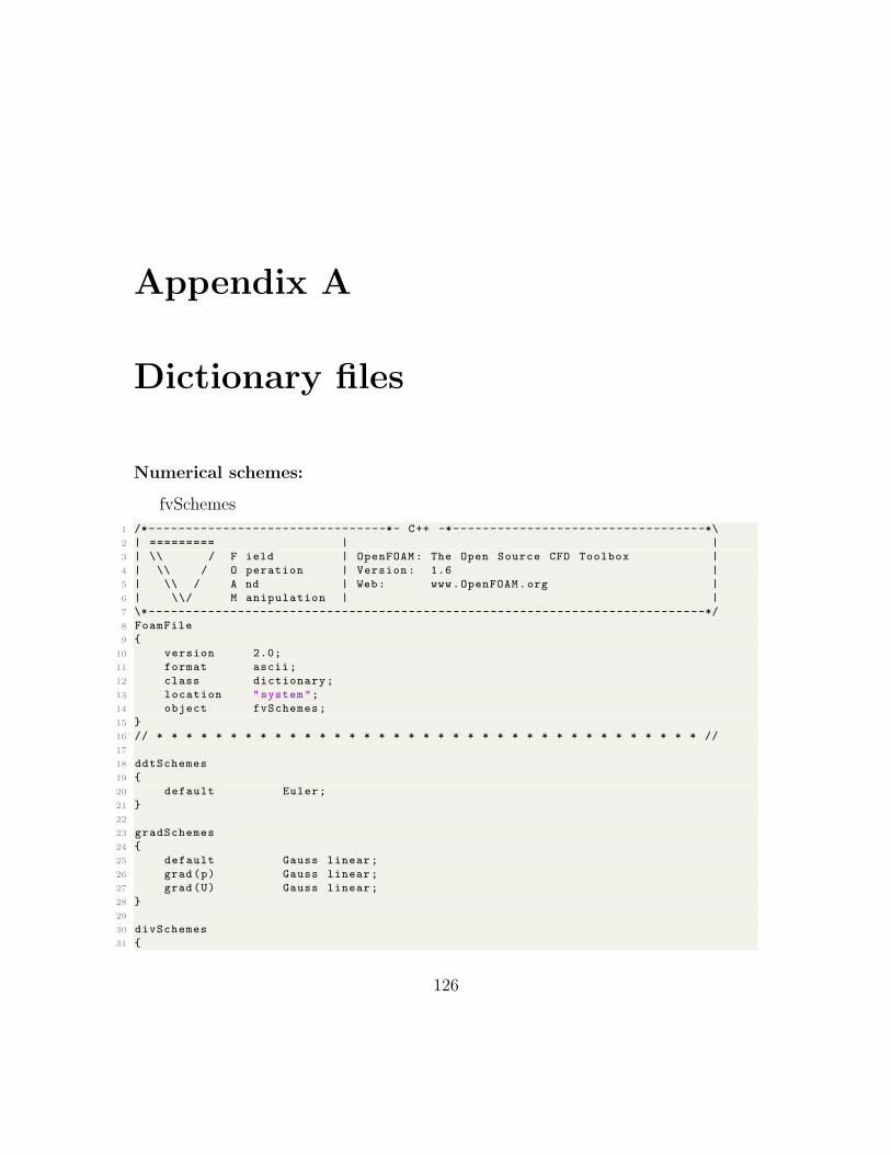
Appendix A
Dictionary files
Numerical schemes:
fvSchemes
1 /*--------------------------------*- C++ -*----------------------------------*\
2 | ========= | |
3 | \\ / F ield | OpenFOAM: The Open Source CFD Toolbox |
4 | \\ / O peration | Version: 1.6 |
5 | \\ / A nd | Web: www.OpenFOAM.org |
6 | \\/ M anipulation | |
7 \*---------------------------------------------------------------------------*/
8 FoamFile
9 {
10 version 2.0;
11 format ascii;
12 class dictionary;
13 location "system";
14 object fvSchemes;
15 }
16 // * * * * * * * * * * * * * * * * * * * * * * * * * * * * * * * * * * * * * //
17
18 ddtSchemes
19 {
20 default Euler;
21 }
22
23 gradSchemes
24 {
25 default Gauss linear;
26 grad(p) Gauss linear;
27 grad(U) Gauss linear;
28 }
29
30 divSchemes
31 {
126
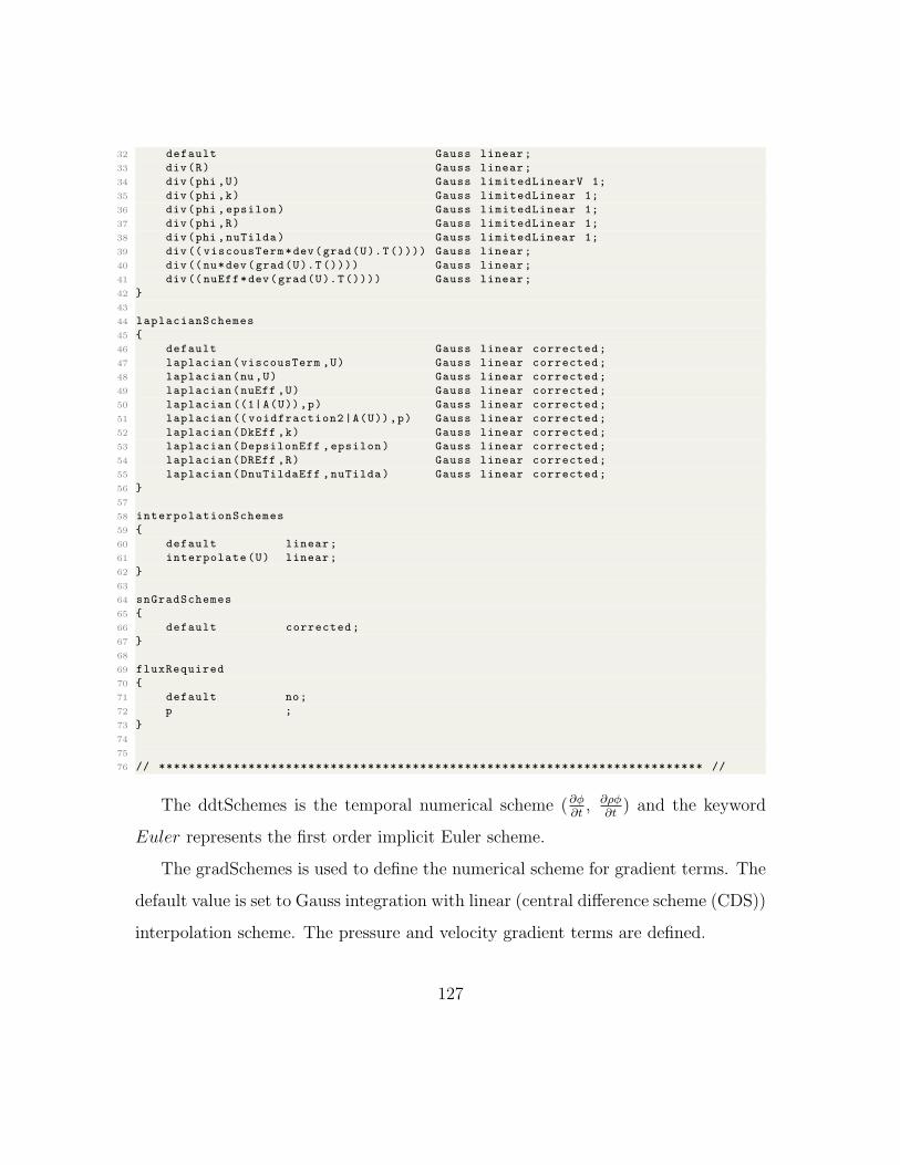
32 default Gauss linear;
33 div(R) Gauss linear;
34 div(phi ,U) Gauss limitedLinearV 1;
35 div(phi ,k) Gauss limitedLinear 1;
36 div(phi ,epsilon) Gauss limitedLinear 1;
37 div(phi ,R) Gauss limitedLinear 1;
38 div(phi ,nuTilda) Gauss limitedLinear 1;
39 div(( viscousTerm*dev(grad(U).T()))) Gauss linear;
40 div((nu*dev(grad(U).T()))) Gauss linear;
41 div(( nuEff*dev(grad(U).T()))) Gauss linear;
42 }
43
44 laplacianSchemes
45 {
46 default Gauss linear corrected;
47 laplacian(viscousTerm ,U) Gauss linear corrected;
48 laplacian(nu ,U) Gauss linear corrected;
49 laplacian(nuEff ,U) Gauss linear corrected;
50 laplacian ((1|A(U)),p) Gauss linear corrected;
51 laplacian (( voidfraction2|A(U)),p) Gauss linear corrected;
52 laplacian(DkEff ,k) Gauss linear corrected;
53 laplacian(DepsilonEff ,epsilon) Gauss linear corrected;
54 laplacian(DREff ,R) Gauss linear corrected;
55 laplacian(DnuTildaEff ,nuTilda) Gauss linear corrected;
56 }
57
58 interpolationSchemes
59 {
60 default linear;
61 interpolate(U) linear;
62 }
63
64 snGradSchemes
65 {
66 default corrected;
67 }
68
69 fluxRequired
70 {
71 default no;
72 p ;
73 }
74
75
76 // ************************************************************************* //
The ddtSchemes is the temporal numerical scheme (∂φ∂t, ∂ρφ
∂t) and the keyword
Euler represents the first order implicit Euler scheme.
The gradSchemes is used to define the numerical scheme for gradient terms. The
default value is set to Gauss integration with linear (central difference scheme (CDS))
interpolation scheme. The pressure and velocity gradient terms are defined.
127
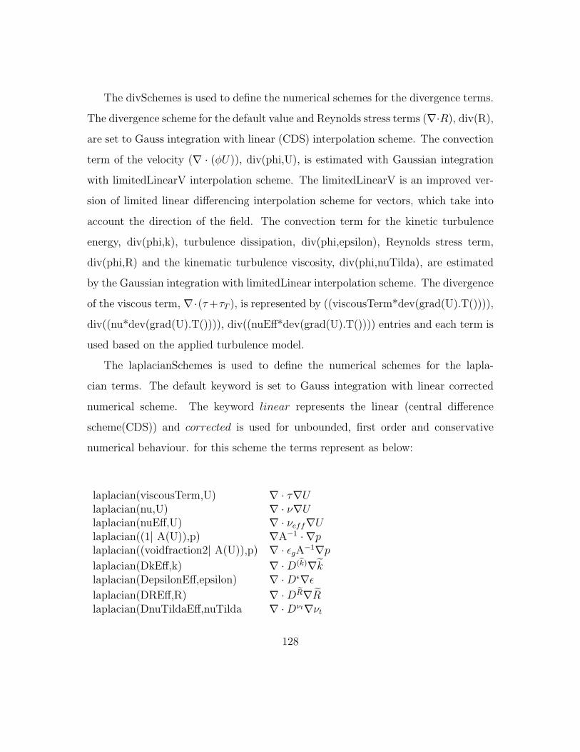
The divSchemes is used to define the numerical schemes for the divergence terms.
The divergence scheme for the default value and Reynolds stress terms (∇·R), div(R),
are set to Gauss integration with linear (CDS) interpolation scheme. The convection
term of the velocity (∇ · (φU)), div(phi,U), is estimated with Gaussian integration
with limitedLinearV interpolation scheme. The limitedLinearV is an improved ver-
sion of limited linear differencing interpolation scheme for vectors, which take into
account the direction of the field. The convection term for the kinetic turbulence
energy, div(phi,k), turbulence dissipation, div(phi,epsilon), Reynolds stress term,
div(phi,R) and the kinematic turbulence viscosity, div(phi,nuTilda), are estimated
by the Gaussian integration with limitedLinear interpolation scheme. The divergence
of the viscous term, ∇·(τ+τT ), is represented by ((viscousTerm*dev(grad(U).T()))),
div((nu*dev(grad(U).T()))), div((nuEff*dev(grad(U).T()))) entries and each term is
used based on the applied turbulence model.
The laplacianSchemes is used to define the numerical schemes for the lapla-
cian terms. The default keyword is set to Gauss integration with linear corrected
numerical scheme. The keyword linear represents the linear (central difference
scheme(CDS)) and corrected is used for unbounded, first order and conservative
numerical behaviour. for this scheme the terms represent as below:
laplacian(viscousTerm,U) ∇ · τ∇Ulaplacian(nu,U) ∇ · ν∇Ulaplacian(nuEff,U) ∇ · νeff∇Ulaplacian((1| A(U)),p) ∇A−1 · ∇plaplacian((voidfraction2| A(U)),p) ∇ · εgA−1∇p
laplacian(DkEff,k) ∇ ·D(k)∇klaplacian(DepsilonEff,epsilon) ∇ ·Dε∇ε
laplacian(DREff,R) ∇ ·DR∇Rlaplacian(DnuTildaEff,nuTilda ∇ ·Dνt∇νt
128

• A−1 is the inverse of the diagonal elements in the discretised momentum equa-
tion.
• D(k) is the diffusion coefficient of the turbulence kinetic energy.
• Dε is the diffusion coefficient of the turbulence kinetic energy dissipation.
• DR is the diffusion coefficient of the Reynolds stress tensor.
• Dνt is the diffusion coefficient of the turbulence viscosity.
The snGradSchemes is used to define the surface normal gradients and the corrected
scheme is used , which represents an explicit non orthogonal correction for the surface
normal gradients.
The fluxRequired is used to define fields which are required to generate the flux.
The pressure field flux is define to be generated.
129
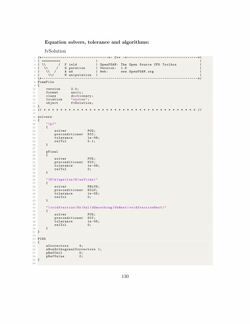
Equation solvers, tolerance and algorithms:
fvSolution1 /*--------------------------------*- C++ -*----------------------------------*\2 | ========= | |3 | \\ / F ield | OpenFOAM: The Open Source CFD Toolbox |4 | \\ / O peration | Version: 1.6 |5 | \\ / A nd | Web: www.OpenFOAM.org |6 | \\/ M anipulation | |7 \*---------------------------------------------------------------------------*/8 FoamFile9 {
10 version 2.0;11 format ascii;12 class dictionary;13 location "system";14 object fvSolution;15 }16 // * * * * * * * * * * * * * * * * * * * * * * * * * * * * * * * * * * * * * //17
18 solvers19 {20 "(p)"21 {22 solver PCG;23 preconditioner DIC;24 tolerance 1e-06;25 relTol 0.1;26 }27
28 pFinal29 {30 solver PCG;31 preconditioner DIC;32 tolerance 1e-06;33 relTol 0;34 }35
36 "(U|k|epsilon|R|nuTilda)"37 {38 solver PBiCG;39 preconditioner DILU;40 tolerance 1e-05;41 relTol 0;42 }43
44 "(voidfraction|Us|Ksl|dSmoothing|UsNext|voidfractionNext)"45 {46 solver PCG;47 preconditioner DIC;48 tolerance 1e-05;49 relTol 0;50 }51 }52
53 PISO54 {55 nCorrectors 4;56 nNonOrthogonalCorrectors 1;57 pRefCell 0;58 pRefValue 0;59 }60
130

61
62 // ************************************************************************* //
131
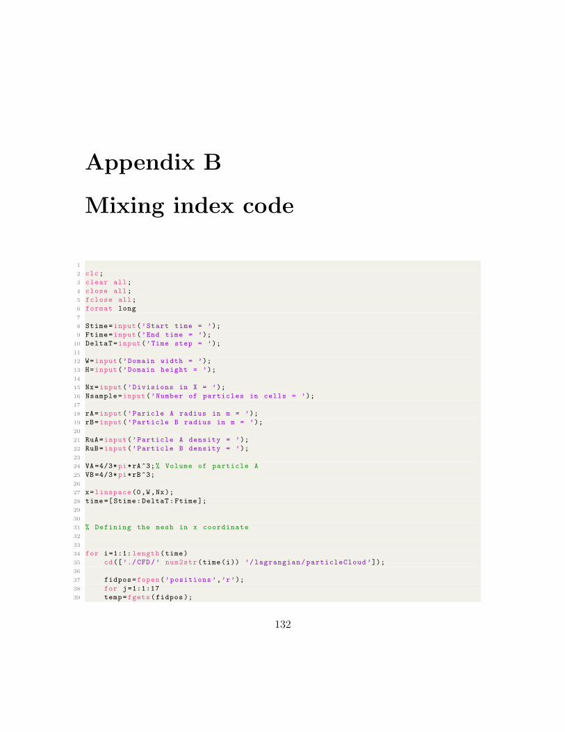
Appendix B
Mixing index code
1
2 clc;
3 clear all;
4 close all;
5 fclose all;
6 format long
7
8 Stime=input(’Start time = ’);
9 Ftime=input(’End time = ’);
10 DeltaT=input(’Time step = ’);
11
12 W=input(’Domain width = ’);
13 H=input(’Domain height = ’);
14
15 Nx=input(’Divisions in X = ’);
16 Nsample=input(’Number of particles in cells = ’);
17
18 rA=input(’Paricle A radius in m = ’);
19 rB=input(’Particle B radius in m = ’);
20
21 RuA=input(’Particle A density = ’);
22 RuB=input(’Particle B density = ’);
23
24 VA =4/3* pi*rA^3;% Volume of particle A
25 VB =4/3* pi*rB^3;
26
27 x=linspace(0,W,Nx);
28 time=[ Stime:DeltaT:Ftime ];
29
30
31 % Defining the mesh in x coordinate
32
33
34 for i=1:1: length(time)
35 cd([’./CFD/’ num2str(time(i)) ’/lagrangian/particleCloud ’]);
36
37 fidpos=fopen(’positions ’,’r’);
38 for j=1:1:17
39 temp=fgets(fidpos );
132
40 end
41 temp=textscan(fidpos ,’%f\n’ ,1);
42 TotPar(i)=temp {1};
43 temp=fgets(fidpos );
44 temp=textscan(fidpos ,’%1s %f %f %f %1s %f\n’);
45 Pos{i}=[ temp {2}(1:end -1,1) temp {3}(1:end -1,1) temp {4}(1:end -1 ,1)];
46
47
48 fidr=fopen(’r’,’r’);
49 for j=1:1:18
50 temp=fgets(fidr);
51 end
52 temp=fgets(fidr);
53 temp=fgets(fidr);
54 temp=textscan(fidr ,’%f\n’);
55 r{i}=temp {1};
56
57
58
59 sampN=TotPar ./ Nsample;
60
61
62
63
64 for j=1:1: length(x)-2
65 ParIndx{i}{j}= find(Pos{i}(:,1)>=x(j) & Pos{i}(:,1)<x(j+1));
66 ParIndxCount(i,j)= length(ParIndx{i}{j});
67 end
68 j=length(x)-1;
69 ParIndx{i}{j}= find(Pos{i}(:,1)>=x(j) & Pos{i}(:,1)<x(j+1));
70 ParIndxCount(i,j)= length(ParIndx{i}{j});
71
72
73 Ny=floor(ParIndxCount/Nsample );
74
75
76
77
78 for j=1:1: length(x)-1
79 [yValue ParIndy{i}{j}]= sort(Pos{i}( ParIndx{i}{j} ,2));
80 end
81
82
83
84 for j=1:1: length(x)-1
85 for k=1:1: Ny(i,j)
86 Cell{i}{j}(:,k)= ParIndx{i}{j}( ParIndy{i}{j}...
87 ((k-1)* Nsample +1:k*Nsample ));
88 end
89 end
90
91
92
93 for j=1:1: length(x)-1
94 for k=1:1: Ny(i,j)
95 NA{i}{j}(k)=sum(r{i}(Cell{i}{j}(:,k))==rA);
96 NB{i}{j}(k)=sum(r{i}(Cell{i}{j}(:,k))==rB);
97 end
133
98 end
99
100
101
102 for j=1:1: length(x)-1
103 for k=1:1: Ny(i,j)
104 temp=NA{i}{j}(k)+NB{i}{j}(k);
105 fracA{i}{j}(k)= NA{i}{j}(k)/temp;
106 fracB{i}{j}(k)=NB{i}{j}(k)/temp;
107 end
108 end
109
110
111
112 meanfracA(i)=0;
113 meanfracB(i)=0;
114 for j=1:1: length(x)-1
115 for k=1:1: Ny(i,j)
116 meanfracA(i)= meanfracA(i)+ fracA{i}{j}(k);
117 meanfracB(i)= meanfracB(i)+ fracB{i}{j}(k);
118 end
119 end
120 meanfracA(i)= meanfracA(i)/sum(Ny(i ,:));
121 meanfracB(i)= meanfracB(i)/sum(Ny(i ,:));
122
123
124
125 stdfracA(i)=0;
126 stdfracB(i)=0;
127 for j=1:1: length(x)-1
128 for k=1:1: Ny(i,j)
129 stdfracA(i)= stdfracA(i)+( fracA{i}{j}(k)-meanfracA(i)).^2;
130 stdfracB(i)= stdfracB(i)+( fracB{i}{j}(k)-meanfracB(i)).^2;
131 end
132 end
133 stdfracA(i)= stdfracA(i)/sum(Ny(i ,:));
134 stdfracB(i)= stdfracB(i)/sum(Ny(i ,:));
135
136
137
138 clear Pos r yValue Ny ParIndx ParIndxCount ...
139 ParIndy fracA fracB temp NA NB Cell
140 fclose all;
141 cd ../../../..
142 end
143
144 sigr=meanfracA .*(1- meanfracA )./ Nsample;
145 sig0=meanfracA .*(1- meanfracA );
146 sigA=stdfracA;
147 sigB=stdfracB;
148
149
150
151 MIA=(sig0 -sigA )./(sig0 -sigr);
152
153
154 figure;
155 hold on;
134

156 plot(time ,MIA ,’k-o’)
157 title(’Lacey mixing index in time’)
158 xlabel(’Time s’)
159 ylabel(’Lacey Mixing Index ’)
160 print(’MI_’,’-depsc ’)
161 CSV=[time ’,MIA ’]
162 csvwrite(’MI’,CSV)
135