Embed Size (px)
Citation preview
Numerical modelling of separated fluid flow over flexible structural membranes
report submitted for transfer from MPhil to PhD
under the supervision of C J K Williams and D Greaves
Lisa Matthews
Department of Architecture and Civil Engineering
University of Bath
August 2005

Contents
i
1 Introduction
1.1 Examples of fluid & flexible structure interaction 1
1.2 Current design practises and wind tunnel testing 2
1.3 Numerical modelling 4
2 Background
2.1 Fluid behaviour 5
2.1.1 Classification of flows
2.1.2 Viscosity
2.1.4 Boundary layer & separation
2.2 Equations of motion for a fluid 12
2.2.1 General conservation law
2.2.2 Conservation of mass
2.2.3 Conservation of momentum
2.2.4 The Navier-Stokes equations
2.3 Turbulence 17
2.4 Design and behaviour of tensile structures 19
2.4.1 Principles of design and analysis
2.4.2 Stability and prestress
2.5 Aeroelasticity of flexible lightweight structures 22
2.5.1 Important aerodynamic effects
2.5.2 Impact of structural response
2.6 Modelling of fluids 25
2.6.1 Flow solution approaches
Particle methods
Potential flow models and stream function formulations
Navier-Stokes primitive variable models
Semi Implicit method for pressure linked
equations – (SIMPLE)
Pressure-implicit with splitting of operators –
(PISO)
Artificial compressibility methods
2.6.2 Discretisation methods
Contents
ii
Finite difference methods
Finite element methods
Finite volume methods
2.6.3 Turbulence modelling
Direct numerical simulation
Large eddy simulation
Reynolds-averaged Navier-Stokes (RANS) system
2.7 Modelling of structures 43
2.7.1 Physical modelling
2.7.2 Numerical modelling
Dynamic relaxation
Application to fabric structures
Application to cable net structures
2.7.3 Aeroelastic analysis
2.8 Computational meshes 50
2.8.1 Types of computational mesh
Structured
Unstructured
2.8.2 Complex geometries and moving boundaries
3 Literature of applications
3.1 Membrane airfoils & sails 54
3.2 Flexible filaments & flags 59
3.3 Parachutes & airbags 61
3.4 Tensile fabric structures 65
4 Literature of finite volume incompressible flow models using
unstructured arbitrary grids
4.1 Variable storage 68
4.1.1 Cell-based control volume, cell-centred variable storage
4.1.2 Vertex-based control volume, cell-centred variable storage
4.2 Interpolation & stability 75
4.3 Pressure-velocity decoupling 77
4.3.1 Staggered grids

Contents
iii
4.3.2 Higher accuracy of pressure gradient derivation
4.4 Unstructured non-orthogonal grids 80
5 Literature of approaches to coupling and interfacing
5.1 Comparison of the behaviour of the two systems 84
5.2 Timestepping 85
5.3 Interface grid conditions 87
5.4 Coupling 89
5.4.1 Monolithic solution
5.4.3 Partitioned solution
6 Literature of boundary conforming mesh moving methods
6.1 Pseudo-solid approach 95
6.2 Lineal and torsional spring models 99
6.3 Transfinite interpolation methods 104
7 Current model and test cases
7.1 Development of the discretisation method for the Navier-Stokes
equations 109
7.2 Solution for pressure 115
7.2.1 To derive the velocity correction formulae
7.2.2 To derive the equation for pressure correction
7.3 Implementation of boundary conditions 121
7.4 Channel flow test case 124
7.4.1 Definition of the test problem
7.4.2 Results
u-velocity
v-velocity
Continuity – conservation of mass
Pressure
7.5 Moving mesh investigations 134
8 Proposed changes to current model and further test cases
8.1 Test case with separation 136

Contents
iv
8.2 Test case with mesh motion 138
8.3 Test case with fluid-structure interaction 140
9 References
Introduction
1
1 Introduction
1.1 Examples of fluid & flexible structure interaction
To understand the mechanisms of interaction between flexible structures and fluid
flow around them is of significant importance in many fields of engineering, such as
the design of sails, flags, parachutes, airbags, fabric building structures and membrane
airfoils for micro-lightweight aircraft. Biological applications for example blood flow
and aneurysm formation, and the swimming techniques of amoeba or other aquatic
invertebrates are further examples of complex fluid-structure interaction mechanisms.
The fundamental feature linking such diverse fields of study is that of the flexible
nature of the structure or membrane involved. Forces generated by the fluid flow
induce not only motion but particularly also deformation of the structure due to its
flexibility. This changes the fluid domain and fluid flow characteristics, in turn
changing the forces on the structure in a continuous feedback loop.
In structural engineering, the behaviour of long-span bridges, tensile surface
structures and tall towers also exhibits similar interaction between the structure and
the fluid flow around it. Of further significance is the fact that the design of such
structures is generally driven by factors other than their aerodynamic performance and
as such they are often aerodynamically ‘bluff’. This results in flow around the
structures that can be highly complex, while the stability of the surface is imparted by
other mechanisms which do not rely on aerodynamic phenomena.
This study will focus on the modelling of the aeroelasticity of architectural
engineering structures, such as tensile fabric surface structures, which, while being
highly flexible and displaying aeroelastic interaction with the surrounding flow, will
not undergo the extreme deformations exhibited by, for example, flags (where
surface-surface contact is possible) but will nevertheless undergo significant
displacements and deformations. Where the Mach number of the flow (ratio of wind
speed to speed of sound in air) remains below 0.3, the flow can be considered to be
incompressible with changes in density negligible. This will be the case for the
structures considered.
Introduction
2
1.2 Current design practices and wind tunnel testing
When considering the wind loading on a structure for design purposes, the approach
taken by both the British Standards and the EuroCode is to consider the surface of the
building to be rigid. Factors such as local wind speed characteristics, local terrain
characteristics and building orientation are used to derive equivalent static pressures
to apply to different zones of the structure based on its shape and form. This
approach is sufficient if the structure will not deform too much under the applied load,
if no dynamic response is excited or if buffeting effects are to be neglected.
For structures outside the applicability limits of the standards, i.e. those deemed too
flexible to assume static pressure approach, wind tunnel tests on a model of the
structure are undertaken in order to derive pressure coefficients at important locations
on the surface. The tests must be designed so that they recreate as accurately as
possible the in-service conditions and behaviour of the structure.
The air flow in the tunnel must resemble the nature of the wind that the structure will
experience. This is difficult to achieve since real wind varies with height, is turbulent
and contains short-duration higher-velocity gusts. Thus a statistical approach to the
wind design environment is most often undertaken, and obstacles are introduced
upstream to try to introduce turbulence and to try to achieve the correct velocity
profile between the mean and gust wind speeds. In order to translate the results from
a wind tunnel test to a full-size structure similarity of Reynolds number can be
employed, however the determination of the characteristic flow speed within the
tunnel is difficult.
The design of the structure model is equally important. If the structure is likely to
move very slowly or very little with respect to the wind speed (i.e. so angles of attack
remain approximately constant) then a rigid model can be used, instrumented to find
wind pressures rather than displacements. However, this is only applicable in cases
where it is safe to assume no aeroelastic interaction.
If aeroelastic interactions are to be reproduced the model must represent the elastic
properties of the structure in an appropriately scaled manner. In addition, it is
Introduction
3
important to ensure that any additional support structure needed does not interfere
with the flow around the model.
Instrumentation of the model must be carried out in such a way as to not interfere with
the flow around the structure, and digital pressure sensors are used to obtain time
history information. The location of the sensors must be carefully chosen to ensure
that areas where energy is most readily extracted from the flow are monitored. It is
not always obvious, however, where these locations are. In addition, it is important to
measure the pressure at more than one pressure sensor simultaneously to obtain
information about the cross-correlation between pressures.
Introduction
4
1.3 Numerical modelling
Due to the above challenges involved in accurate wind tunnel testing of aeroelastic
behaviour, along with the large expense involved, interest has grown in the area of
numerically modelling such phenomenon. In all but the simplest of cases an
analytical solution for the behaviour of the interacting structure and fluid is not
available and so numerical computational methods are employed.
It is easier to include more of the surrounding terrain in a computational model than in
a wind tunnel, and easier to ensure that particular flow conditions are maintained.
Similarity of all parameters can be ensured and the resulting loads and displacements
of the structure can be extracted directly. However, the challenge now becomes
finding a method to validate a particular computational code through comparisons
with experimental results or other numerical methods.
The numerical simulation of aeroelastic interaction requires significant computational
power and expense; three systems are being managed – the fluid flow, the structure,
and the fluid-structure interface.
The equations of motion become further complicated in the unsteady case where the
boundaries of the domain are moving; the simultaneous solution of equations
describing fluid, structure and dynamic mesh is challenging. The model must also be
able to provide accurate results despite the large displacements and deformations of
the fluid-structure boundary. Numerical grid generation (including re-meshing or
mesh adaptation), coupling and interfacing often require more computational effort
than solving the equations of motion.
Background
5
2 Background
2.1 Fluid behaviour
A fluid is a material which cannot support shear stresses without undergoing motion;
an element of fluid will always deform under shearing action. Liquids and gases are
both fluids, and their behaviour can be described by the same equations of motion
despite significant differences in their physical properties. The application of external
forces will cause a fluid to flow. Pressure gradients and gravity are the most common
causes of flow, and properties of the fluid, in particular density and viscosity, are very
important in determining how the fluid behaves under these forces. Firstly a number
of ways of categorising different flows shall be defined.
2.1.1 Classification of flows
While all fluids are made up of individual fluid molecules, the Kinetic Theory of
Gases (see for example Loeb (2004)) allows us to describe the macroscopic properties
of the fluid (or a piece of the fluid) in terms of the microscopic activity. The
characteristics of the flow (e.g. velocity, pressure, density) are in general not constant
in time and space. The continuum model approach considers average values of these
variables by treating the fluid as a continuum rather than as molecules with relatively
large areas of empty space in between. The average values of the fluid parameters are
over very small elements of fluid, but these contain a very large number of molecules,
so the continuum hypothesis is still valid.
If the flow parameters at any point in the flow do not change with time, then the flow
is termed steady. The equations of motion (as we shall see later) contain no time
derivative terms. If, however, the variables at a point do change with time the flow is
termed unsteady or non-steady. The distinction between steady or unsteady flow can
vary depending on the position of the observer, since all motion is relative. Steady
flow is much easier to analyse than unsteady flow, but in practice steady flow does
not occur very often. Steady flow analysis can be considered to be a form of unsteady
analysis which is caused to converge on an equilibrium state.
Background
6
If, at a particular instant in time, a flow parameter does not vary over a region of the
domain, the flow is termed uniform in that region. If variation of a parameter does
occur over a region then the flow is termed non-uniform. In this case it is important
to consider variations of flow parameters not only in the direction of the flow, but also
perpendicular to it, e.g. variations normal to the flow direction at a solid boundary due
to viscosity.
Streamlines, streaklines and particle paths can be used in order to study the nature of
the flow. A streamline is a curve in space along which the flow is always tangential.
There is thus no flow across a streamline and streamlines can never cross or intersect.
Streamlines can be considered as a snapshot representation of the flow velocity field
at one instant in time. Individual particles will not necessarily follow streamlines. If
the location of one given particle is plotted over a series of time instants then a
particle path is generated. The particle path can be considered as a particle trajectory
through the domain. Streaklines are constructed by mapping the location at a given
instant of every particle that has passed through a particular point in the domain since
a starting time. Experimentally streaklines are created in wind tunnels using smoke
particles or in flumes using dye. In general, streamlines, streaklines and particle paths
will be different for a given flow regime. Only in the case of steady flow will all
three coincide.
At low flow speeds, the fluid particles move in smooth paths, following directly the
particle downstream, with lines of flow never crossing. This is called laminar flow.
Although the flow velocity can be different from one line to the next, the velocity
varies smoothly throughout the domain. If the flow velocity is increased, the laminar
regime can be maintained up to a point, after which the flow variables begin to
fluctuate in a random manner. Eventually, each fluid particle follows its own path
which crosses over the paths of other particles and thorough mixing of the flow
occurs. The flow regime is now termed turbulent, the transition is known as the
onset of turbulence, and has been the focus of study of many fluid dynamicists for
over one hundred years.
The general flow direction is thus the average velocity of all the particles, each fluid
particle now behaves with a random velocity superimposed on the general flow
Background
7
direction, following an erratic three-dimensional path. A complete mathematical
description of turbulent flow has still not been achieved; closure models are
introduced instead to describe the transport and dissipation of turbulent kinetic energy
in a statistical sense. Almost all flows of engineering significance are turbulent.
The Reynolds number of the flow can be used to give an idea of the nature of the flow
regime in the laminar-turbulent spectrum. It is also useful for comparing different
flows in a non-dimensionalised way. The Reynolds number is defined as:
υµρ UDUD
==Re [2-1],
where ρ is the density of the fluid, U a characteristic velocity (the free-stream
velocity is generally used), D is a characteristic length scale (such as the diameter of
a cylinder in the flow), µ is the dynamic viscosity of the fluid, and υ the kinematic
viscosity of the fluid.
The Reynolds number can be thought of as a measure of the relative importance of
interial forces compared to the viscous forces. Two different flows having the same
Reynolds number ought to exhibit similar flow characteristics in terms of the laminar
/ turbulent nature.
2.1.2 Viscosity
Shear deformation can be considered as the relative movement of one layer of fluid
particles over an adjacent layer. All fluids exhibit some resistance to this shearing
deformation, some more than others. The shear stress resulting from the deformation
can be related to the rate of shear via the coefficient of viscosity:
shear stress = dynamic viscosity x rate of shear strain
Considering the case of two-dimensional steady flow in the x-direction of layers of
fluid having different velocities relative to each other, the shear stress between the
layers is:
y
u
∂∂
= µτ [2-2],
Background
8
where τ is the shear stress between the layers, µ is the dynamic viscosity, u is the
flow velocity in the x-direction and y is the coordinate direction normal to the flow.
For a Newtonian fluid at a given temperature, the coefficient of viscosity is constant
i.e. independent of the rate of shear.
The above definition of the relationship between shear stress and rate of shear strain
demonstrates a number of important points. Firstly, shear stress is zero when there is
no relative movement between adjoining layers of fluid. Secondly, the velocity
gradient must always be finite since otherwise infinite stress would occur. This
implies that velocities must vary continuously throughout the domain. This condition
also applies at a solid boundary where the fluid immediately in contact with the
boundary must have the same velocity as the boundary, or else a step-change in
velocity would be occurring. This is known as the condition of no-slip at the
boundary. The no-slip condition must be satisfied in a continuum model of a viscous
fluid. For a detailed description of the theoretical and experimental justification of the
no-slip condition see Prabhakara & Deshpande (2004).
It is due to viscosity that energy must be continuously supplied to maintain a fluid
flow. Energy is required to overcome this internal friction due to the viscous forces; it
is then dissipated as heat.
At the molecular level, viscosity of a liquid can be attributed to two mechanisms:
⋅ inter-molecular forces resisting the relative motion
⋅ thermal agitation causing migration of particles between adjacent fluid layers which
has the effect of transporting momentum between the layers
Considering a gas, the second mechanism is much more important since the distances
between particles are so large that the intermolecular forces can be considered
negligible. This is supported by the kinetic theory of gases and experimental
observation, which demonstrate that the viscosity of a gas is independent of its
pressure but not of its temperature (since this increases thermal agitation).
Background
9
In considering the behaviour of different flows, we are often concerned with the
relative influence of viscous forces to inertial forces. In these cases it is useful to
consider the ratio of viscosity to density – known as the kinematic viscosity.
2.1.3 Boundary layer & separation
The no-slip boundary condition at a solid wall causes the generation of a region of
fluid next to the wall where the flow velocity increases rapidly towards the free-
stream velocity. This region is known as the boundary layer, and is most often
defined as the region over which the fluid achieves 90% of the free stream velocity.
In this region viscous forces are important compared to the inertial forces since the
velocity gradients are highest here while the velocities (and hence momentum) are
lowest. The boundary layer region must form in flow of all viscous fluids, regardless
of the Reynolds number of the flow.
In real engineering flows, however, it is highly unlikely that this boundary layer
remains attached to the solid wall along its entire length. Prandtl first recognised that
the behaviour of the boundary layer is highly sensitive to the variations of pressure in
the region. If the fluid pressure decreases downstream along the boundary, then the
boundary layer remains attached to the wall. If, however, an adverse pressure
gradient exists – one of increasing pressure downstream, then the boundary layer may
separate from the solid surface. This occurs since the fluid nearest to the wall has
very low velocity compared to that further out and thus has relatively low kinetic
energy. There reaches a point in the boundary layer where the momentum of the fluid
is insufficient to overcome the adverse pressure gradient, which thus may bring the
fluid to rest. Fluid even nearer to the wall than this point may in fact be forced by the
pressure gradient to move in the opposite direction to the main flow, thus forming a
region of reversed or ‘recirculating’ flow near to the wall.
Background
10
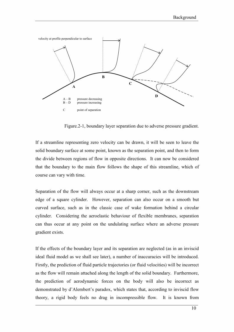
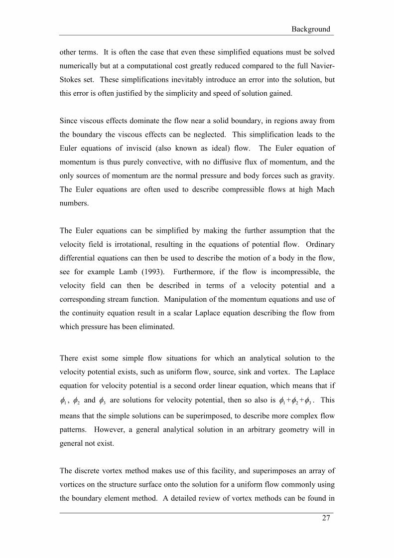
Figure.2-1, boundary layer separation due to adverse pressure gradient.
If a streamline representing zero velocity can be drawn, it will be seen to leave the
solid boundary surface at some point, known as the separation point, and then to form
the divide between regions of flow in opposite directions. It can now be considered
that the boundary to the main flow follows the shape of this streamline, which of
course can vary with time.
Separation of the flow will always occur at a sharp corner, such as the downstream
edge of a square cylinder. However, separation can also occur on a smooth but
curved surface, such as in the classic case of wake formation behind a circular
cylinder. Considering the aeroelastic behaviour of flexible membranes, separation
can thus occur at any point on the undulating surface where an adverse pressure
gradient exists.
If the effects of the boundary layer and its separation are neglected (as in an inviscid
ideal fluid model as we shall see later), a number of inaccuracies will be introduced.
Firstly, the prediction of fluid particle trajectories (or fluid velocities) will be incorrect
as the flow will remain attached along the length of the solid boundary. Furthermore,
the prediction of aerodynamic forces on the body will also be incorrect as
demonstrated by d’Alembert’s paradox, which states that, according to inviscid flow
theory, a rigid body feels no drag in incompressible flow. It is known from
A
B
C
D
velocity at profile perpendicular to surface
A – B pressure decreasing
B – D pressure increasing
C point of separation
Background
11
experimental investigation, that, for a bluff body, this is never the case as the flow
does not remain attached. It is also known that separation causes a loss of lift force
(such as during ‘stalling’ of an airfoil) an increase of drag force and variations in
pressure, all of which influence significantly to the mechanisms of aeroelastic
response.
Background
12
2.2 Equations of motion for a fluid
To formulate the equations of motion of a fluid we will take the continuum hypothesis
approach and consider the fluid to be a continuum rather than consider the motion of
each fluid molecule individually. We can then consider the average conditions (of
velocity, pressure, density etc) within a particle or element of fluid.
The element of fluid is generally constructed in a Eulerian fashion, that is where the
fluid (in general) flows through the element being considered. If a Lagrangian
approach was taken, that is where the element contains the same fluid particles from
one time instant to the next, the mesh subdividing the domain would quickly become
tangled.
The aim is to formulate conservation laws for extensive properties of the fluid (that is
properties dependent on the amount of fluid being considered) in terms of
fundamental intensive properties. In this case we will form conservation laws for
mass and momentum of the fluid element in terms of pressure, density and velocity)
by considering the processes at work to change the mass and momentum of the fluid
element. First we will consider a general conservation law.
2.2.1 General conservation law:
Consider an arbitrary element of fluid having volume V bounded by surface S. If φ is
some scalar variable intensive property per unit mass of the fluid (such as pollutant
concentration, density or energy), then the amount of variable φ contained within the
element, the corresponding extensive property, Φ , will be:
∫=ΦV
dV ρφ [2-3].
Φ will change due to fluxes of φ through the bounding surface of the element, or due
to sources of φ acting over the bounding surface or acting on the volume as a whole:
∫∫∫∫ ⋅+=⋅+S
S
V
V
SV
dSdVQdSdVdt
d nQnFρφ [2-4],
Background
13
where F represents fluxes of φ through the surface, S, of the volume, QV are the
volume sources of φ acting over V and QS are surface sources acting over S. Fluxes
contained in the term F can be diffusive (i.e. due to molecular thermal agitation) or
convective (due to transport with the fluid motion) in nature.
If the surface source vector and flux vector are assumed to vary continuously
throughout the field (which is the case here since shocks are not going to be
modelled), then the divergence theorem can be applied to convert the surface integrals
to volume integrals:
∫∫∫∫ ⋅∇+=⋅∇+V
S
V
V
VV
dVdVQdVdVdt
d QFρφ [2-5].
Considering at the limit an arbitrary element, we arrive at the differential form:
( ) VS Qt
=−⋅∇+∂∂
QFρφ
[2-6].
If the conserved variable φ is a vector, a similar conservation law can be written,
wherein the surface fluxes are tensors, the surface sources are tensors and the volume
sources are vectors. The general form of [2-6] still applies.
2.2.2 Conservation of mass:
The starting principle is that mass cannot be created or destroyed in the system.
Further, mass is only transported via convection, not diffusion, and there are no mass
sources (e.g. due to chemical reaction or multiphase flow). This is equivalent to the
statement that mass is not transported in a sourceless fluid at rest. In this case the
variable φ in [2-3] is equal to 1, considering [2-6]:
( ) 0=⋅∇+∂∂
uρρt
or ( ) 0div =+∂∂
uρρt
or ( )
0=∂
∂+
∂∂
i
i
x
u
t
ρρ [2-7],
which, for an incompressible fluid (density constant) reduces to:
0=⋅∇ u or 0 div =u or 0=∂
∂
i
i
x
u [2-8],
and in two-dimensional Cartesian coordinates:
Background
14
0=∂∂
+∂∂
y
v
x
u [2-9].
2.2.3 Conservation of momentum:
It is assumed that no flux of momentum occurs in a fluid at rest; only convective
momentum fluxes exist, that is transport of momentum due to the rate of flow of mass
into / out of the control volume. Sources of momentum are the forces acting on the
element. These can be external forces (also known as body forces) acting on the mass
of the volume (e.g. gravity / buoyancy), or internal forces acting due to internal
deformations of the fluid. Internal forces cancel out at every internal point of the
volume, leaving the out of balance force due to their action at the surface of the
volume, which are thus also known as surface stresses (pressure, normal & shear
stresses, but not in this case surface tension). Surface forces depend on the nature of
the fluid and how it behaves under deformation. In this case, the variable φ in [2-3]
is a vector representing the velocity of the fluid. Considering [2-6]:
( ) ( ) fσuuu
ρρρ
=−⋅∇+∂
∂t
[2-10],
where the first term in the divergence brackets on the left hand side is the convective
flux of momentum through the bounding surface, and the second is the source of
momentum that are the surface stresses.
Surface stresses can thus be thought of from the molecular point of view as fluxes of
momentum across the surface. The surface stresses consist of an pressure component
and a component due to viscous stresses on the surface:
τIσ +−= p [2-11],
which, into [2-10], and in the absence of body forces (such as gravity), yields:
( ) ( )ij
ij
j
jii
x
p
xx
uu
t
u
∂∂
−∂
∂=
∂
∂+
∂
∂ τρρ [2-12].
If we consider a Newtonian model (where viscosity is taken to be constant, which
applies in this case since no extremes of temperature or pressure are to be modelled)
to relate viscous stresses to internal strains, the viscous stresses can be written:
Background
15
∂
∂−
∂
∂+
∂
∂= ij
k
k
i
j
j
iij
x
u
x
u
x
uδµτ
3
2 [2-13],
where ijδ is the Kronecker Delta, which has a value of 0 except when i=j in which
case it is equal to 1.
If in addition the fluid is incompressible, then by [2-8], [2-13] reduces to:
∂
∂+
∂
∂=
i
j
j
iij
x
u
x
uµτ [2-14].
Thus [2-10], in two-dimensional Cartesian coordinates, yields:
( ) ( )x
p
y
u
x
u
y
uv
x
uu
t
u
∂∂
−
∂
∂+
∂
∂=
∂∂
+∂∂
+∂∂
ρυ
12
2
2
2
and ( ) ( )
y
p
y
v
x
v
y
vv
x
uv
t
v
∂∂
−
∂
∂+
∂
∂=
∂∂
+∂∂
+∂∂
ρυ
12
2
2
2
[2-15],
where the coefficient of kinematic viscosity:
ρµ
υ = [2-16].
2.2.4 The Navier-Stokes equations
[2-9] and [2-15] together are the Navier-Stokes equations of motion for the flow of an
incompressible Newtonian fluid in two-dimensions. The equations are closely
coupled – each velocity component occurs in each momentum equation [2-15] and the
continuity equation [2-9]. The momentum equations contain non-linear convection
terms which render the system non-self-adjoint. It is difficult to treat these convective
fluxes conservatively (explicitly) since they are products of unknown velocities at the
face of the element.
The fluid pressure appears in both momentum equations but not in the continuity
equation, the system thus contains no independent equation for pressure although this
is one of the unknowns. If the fluid were compressible, then the pressure can be
related to density and temperature via the equation of state, however no such
expression can be formulated here since the density is taken to remain constant. Thus
Background
16
the role of the pressure terms in the equations becomes that of a constraint on the
solution – if the correct pressure field is applied to the momentum equations then the
resulting velocity field should satisfy continuity.
It is very difficult to solve the Navier-Stokes system analytically in all but simplest of
cases (e.g. laminar flows in simple geometries) in these cases the system is solvable
since many terms are zero. In some other cases it is possible to make some
assumptions about the flow and to neglect some terms which are small compared to
others to form simplified equations. These assumptions introduce errors into the
solution. However this approach is justified if, even if the equations must still be
solved numerically (rather than analytically), the computational effort is generally
much smaller than for the full system.
Background
17
2.3 Turbulence
The Navier-Stokes equation system is valid for flow of a viscous Newtonian fluid. As
previously described, in reality the flow stays laminar up to a point then becomes
turbulent. The Reynolds number, Re, at which this transition occurs is known as the
critical Reynolds number.
Turbulent flow contains a very broad range of temporal and spatial scales of activity,
and therefore also broad energy spectrum. The largest eddies carry most of the
turbulent kinetic energy and are responsible for turbulent diffusion. They are
dominated by inertia effects; viscous effects are negligible. They are of a scale of
similar order of magnitude as the length scale of the flow (that used to find Re). The
structure of the largest eddies is highly anisotropic since they interact strongly with
the mean flow.
The smallest eddies dissipate turbulent kinetic energy into heat through molecular
viscosity. These eddies are of a scale of the order of the Komolgorov microscale:
41
=ευ
η [2-17],
where ε is the average dissipation rate of turbulent kinetic energy and υ is the
coefficient of kinematic viscosity.
This scale is dictated by the viscosity; here viscous effects dominate. In typical
engineering flows the smallest eddies may be in the range 0.1-0.01mm, with an
associated frequency of variation of motion of around 10kHz (Versteeg &
Malalasekera 1995). This dissipation results in increased internal energy losses in
turbulent flows, and, further, the viscous diffusion tends to smear out the
directionality of the flow resulting in a more isotropic nature of the smallest eddies.
The different scales are mixed together and overlap in the flow. The larger eddies
transport and shed smaller eddies and energy is transferred between different length
scales in highly non-linear way. The transfer of energy progressively down the length
spectrum to its eventual dissipation due to internal friction is known as the energy
cascade.
Background
18
It is essential that any flow model accurately takes into account both the diffusion and
dissipation of turbulent kinetic energy in the flow. Thus the ratio of length scales
which must be resolved to compute directly all lengths of turbulence varies with Re3/4
in 2D (Tennekes & Lumley 1972), and with Re9/4 in 3D (Hartel 1996, Chung 2002).
In the flow region near a solid wall boundary layer the smallest eddy size is
determined by the thickness of the viscous wall layer which requires an even finer
grid resolution. The task for the designer of a computational model of turbulent flow
is to decide what range of length scales the model shall explicitly resolve, and how to
take into account the effects of turbulent activity outside of that range.
Background
19
2.4 Design and behaviour of tensile structures
2.4.1 Principles of design and analysis
The most efficient use of material to carry load is to employ that material to its tensile
capacity. In compressive modes instability effects reduce the overall capacity of the
member once a certain slenderness of the element is reached. This feature has long
been exploited in the design of structures requiring minimum weight; flying
machines, portable structures and large span structures. In addition, an element in
tension may undergo deflections, which would then increase its efficiency in carrying
load. This is known as positive geometric stiffness, and is a predominant feature in
the behaviour of tension structures.
Cable and membrane structures are designed to carry only tensile loads or develop
only tensile stresses. A cable or membrane has effectively zero bending stiffness and
the shape that it adopts is dependent only on the internal tensions and the external
loads; the shape is funicular. Quadrangular cable meshes and fabric membranes have
also effectively zero in-plane shear stiffness.
This characteristic is exploited in tensile surface design; angular distortions of the
surface grid are required in order for a curved geometry to be achieved. In the fabric
membrane case this is true within certain limits of shear strain, after which wrinkling
of the fabric will occur. For this reason, the surface is made up of shaped fabric
panels in order to limit the maximum in-plane shear strain required to generate the
form. A triangular cable net, however, allows no angular distortion of the grid, and so
is much stiffer in plane.
2.4.2 Stability and prestress
The high flexibility of such surfaces (zero bending and zero shear stiffness) leads to
large deflections of the structure under different loads. These deflections are required
in order to carry the applied loads, as it is the curvature and tension in the surface
which resist them. However, it is often also desirable to limit these deflections to
Background
20
within tolerable limits for reasons of sealing, cladding and serviceability of the
structure. Different approaches to this question of stability are now discussed.
A singly curved surface requires sufficient mass and bending stiffness to resist loads
acting to decrease the curvature of the surface. Heavy weight cable roofs consist of a
set of parallel hanging cables carrying cladding such as concrete panels. The panels
are heavy and stiff for the purpose of resisting wind uplift forces.
A double curved anticlastic surface exploits the opposing nature of its curvatures (its
negative Gaussian curvature) to maintain tension in the surface under varying loads.
Deflections of the structure in any direction act to increase curvature in one of the grid
directions, thus maintaining the ability of the surface to support loads.
Prestressed fabric membranes and cable nets use this method for stability. The grid
elements, be they fabric yarns or cables, can be prestressed against each other during
erection. In use the ‘ridge’ elements carry wind uplift, and the ‘valley’ elements the
self weight and snow loads. The simplest and most commonly used anticlastic
surface is the hyperbolic paraboloid, consisting of two sets of intersecting parabolas
of opposing curvatures.
A doubly curved synclastic surface (positive Gaussian curvature) is achieved through
the application of a pressure differential across the membrane surface. Effectively a
further form of prestressing, this pressure differential develops tensile stresses in the
membrane which act to stabilise the surface. This is the basis of design for air-
supported and pneumatic structures.
The relatively large deflections experienced by the surface of the structure, principally
due to the low shear stiffness as described, lead to non-linear equations describing the
equilibrium of the system. For this reason non-linear analysis methods are required to
determine surface stresses and deflections. However, the low bending and shear
stiffness is useful when packing and transporting tension structures; also only
relatively gentle stress variations are experienced in the surface as the structure can
move to accommodate stress differences.
Background
21
A fundamental aim of tensile structure design is to ensure that tensile stresses are
maintained in all elements at all times under normal working loads. It can be
acceptable to lose tension in some areas under extreme loading, provided the integrity
of the whole structure is not threatened.
To ensure slackening does not occur, tension structures are prestressed; to establish a
certain level of tension in the elements which must be overcome by any given loading
condition before relaxation of an element occurs. Prestress levels are also designed to
limit the deflections of the structure by ensuring that the prestress is the primary load
that the elements undergo. This aids the elimination of flutter.
To efficiently impart curvature and prestress into a surface requires careful provision
of supports, internal or external to the surface field, to ensure that sufficient difference
between high and low points exists. In this way, the boundary shape and the
geometry and location of supports for the structure, along with the prestressing levels
required, prescribe the surface which shall be generated in its entirety. Form is a
direct result of function.
Background
22
2.5 Aeroelasticity of flexible lightweight structures
Aeroelasticity is the study of the interactions between the deformations and
displacements of an elastic structure in an airstream and the resulting aerodynamic
forces. When air flows around a structure, aerodynamic effects will result in a force
on the structure which, if possible, will move due to these forces. Since the structure
forms a boundary to the flow, the flow characteristics will be altered due to this
motion, which in turn will change the aerodynamic forces on the structure, in turn
changing its displacements… in a continuous feedback loop.
The result of this aeroelastic interaction can be that the structure moves to find some
new position in which it is in equilibrium with the external forces. However, with
gradually increasing flow speeds, a point may be reached where an aeroelastic
instability occurs: the interaction can cause the motions of the structure to vary in an
oscillatory manner the amplitude of which could be maintained or could grow over
time.
It is important to note that such an unstable response from the structure can occur in a
steady uniform flow. For example, above a certain velocity, vortices are shed from
separation points on a cylinder in a flow in a periodic manner leading to oscillating
forces on the cylinder.
There is much research in the field of aerospace design in order to predict the
dynamic loads and vibrations in elements of aircraft – e.g. helicopter wake and
vertical tail interaction, active aeroelastic wings, panel and wing flutter of space
vehicles. Understanding such behaviour has a direct impact on cost and operational
safety.
Examples of flexible lightweight structures in civil and structural engineering are
tensile fabric or cable net roofs, long-span bridges or tall slender towers. Tensile
roofs rely on interaction of curvature and tension for stability, and rely on geometric
stiffness to resist imposed loads. In general lightweight structures will deform under
applied load to mobilise resistance to the load. Changes in shape lead to changes in
Background
23
stiffness which thus alters the response of structure to further loading. They thus
exhibit highly non-linear structural behaviour.
Such structures also have relatively low self weight which means that other imposed
loads, such as wind loads, are relatively more significant compared to gravity loading.
The low mass also tends to mean that they have low damping of vibrations.
Design of civil and structural engineering lightweight structures is primarily governed
by parameters other than aerodynamic performance (e.g. aesthetics, prestress stability
etc.) which means that they then tend to be aerodynamically bluff. This means that air
will not tend to flow smoothly around the structure, but will tend to deviate from the
surface resulting in large regions of separated and/or turbulent flow, and a large
turbulent wake.
2.5.1 Important aerodynamic effects
The flow around a ‘bluff’ structure will tend to induce pressure variations and
fluctuations across the surface. The pressure will change considerably with time as
structure shape changes, and this can lead to a negative stiffness of the surface where
the pressure variations tend to pull up ridges and push down valleys. The
phenomenon of panel flutter is when these wrinkles tend to oscillate and extract
energy from the flow.
A further important aerodynamic effect which must be considered is separation of the
boundary layer. The flow will tend to separate in regions of adverse pressure
gradient, and the point of separation will move across the surface as the structure
deforms. It is also important to model the (turbulent) wake downstream of separation,
in addition to the shedding of vortices from trailing edge of the structure or locations
of rapid changes in curvature.
In particular we are interested in the limit point where structure can no longer simply
deform into new shape and stay there in equilibrium with applied loads; a loss of
static stability occurs indicating a transition to unsteady response (even in steady
uniform flow).
Background
24
It is generally accepted that the accurate prediction of such phenomenon relies on the
ability of the aeroelastic model to take into account the viscous nature of the flow. If
viscosity is neglected, as is the case in many linearised simplified models for reasons
of computational simplicity then boundary layer effects cannot be modelled since the
no-slip condition (and thus formation of a boundary layer) does not occur. The
thickening and/or separation of the boundary layer at the fluid-structure interface is an
essential aspect of these aeroelastic effects.
2.5.2 Impact of structural response
The response of the structure under these aeroelastic effects will influence many
aspects of structural design. Anchorages and supports must be designed for
maximum loads which may well be associated with these extremes of unsteady
behaviour. Serviceability design dictates permissible limits to the maximum
deflections of the surface, for example in order to ensure the comfort of people in or
near the structure. Since lightweight structures rely on the interactions of tension and
curvature for stability of the surface, it is important to check the limit of structural
behaviour, for example to look for wrinkling of the surface or overstressing of seams.
Background
25
2.6 Modelling of fluids
2.6.1 Flow solution approaches
Particle Methods
For some applications, the approach can be taken to consider the motion of individual
‘packets’ of fluid, rather than make the assumptions of treating the fluid as a
continuum. The equations of motion are then formulated in a Lagrangian fashion
considering the forces on each fluid particle and the equations of conservation.
The most commonly used of these types of methods is the Smoothed Particle
Hydrodynamics approach (SPH) which has been extensively applied to problems in
astrophysics, such as the formation of stars. Early developments were undertaken by
Lucy (1977) and Gingold & Monaghan (1977). A more recent review can be found in
Monaghan (1992).
SPH is particularly suited to this type of problem, since the Lagrangian nature of the
formulation means that the computations are concentrated in areas of the domain
where material is found, and no (or very little) computational time is spent
considering the regions of empty space. A further advantage of the method is that it is
in essence a grid-less method and as such avoids many of the complications of mesh
motion control encountered when using grid-based methods to track the motion of
free surfaces.
To evaluate a flow variable at a point in the domain a specified number of
surrounding particles are taken into account using interpolation or smoothing
functions, known as smoothing kernels. These functions are most commonly
Gaussian functions or cublic spline functions, and the contribution of one particle to
the properties of another particle is thus weighted according to the distance between
them. The property, A, of particle i is thus evaluated:
( )∑ −=j
ji
j
j
ji hWA
mA ,rrρ
[2-18],
Background
26
where j is the number of surrounding particles taken into account, mj is the mass of
the neighbour particle, Aj is the value of the property being considered at the
neighbour particle, jρ is the density associated with the neighbour particle and W is
the smoothing function chosen.
W is a function of the distance between the particles i and j, which is given by ri – rj
where r is the location vector of the particle relative to some fixed point. W is also a
function of h the smoothing length. This parameter governs the range of influence of
each particle. The most common approach is to take into account all particles within
a distance of 2h from the point being considered. The smoothing length need not be
constant over the whole domain, or constant with respect to time. This means that the
resolution of the scheme can be increased in regions where the particles are more
concentrated, and reduced in regions where the particles are far apart. Alternatively,
if a fixed number of smoothing neighbours are used then the same level of accuracy is
achieved throughout the domain.
Spatial derivatives of the flow variables can be found directly from [2-18]:
( )∑ −∇=∇j
ji
j
j
ji hWA
mA ,rrρ
[2-19],
which can be evaluated directly if a smoothing kernel W is chosen which is
differentiable at least once.
In comparison with grid-based schemes, the SPH approach has been found to smear
out shocks and contact discontinuities to a greater degree. Furthermore the SPH
approach is limited to density-based adaptive resolution only since the smoothing
length h is essentially a measure of the mean inter-particle spacing, whereas a grid-
based scheme can adapt the resolution of the solution based on any criterion desired.
Potential flow models and stream function formulations
The analytical solution of the Navier-Stokes equations is very difficult except in a few
of the simplest of cases. These cases generally present flow problems where it is
possible to neglect certain terms in the equations because they are small compared to
Background
27
other terms. It is often the case that even these simplified equations must be solved
numerically but at a computational cost greatly reduced compared to the full Navier-
Stokes set. These simplifications inevitably introduce an error into the solution, but
this error is often justified by the simplicity and speed of solution gained.
Since viscous effects dominate the flow near a solid boundary, in regions away from
the boundary the viscous effects can be neglected. This simplification leads to the
Euler equations of inviscid (also known as ideal) flow. The Euler equation of
momentum is thus purely convective, with no diffusive flux of momentum, and the
only sources of momentum are the normal pressure and body forces such as gravity.
The Euler equations are often used to describe compressible flows at high Mach
numbers.
The Euler equations can be simplified by making the further assumption that the
velocity field is irrotational, resulting in the equations of potential flow. Ordinary
differential equations can then be used to describe the motion of a body in the flow,
see for example Lamb (1993). Furthermore, if the flow is incompressible, the
velocity field can then be described in terms of a velocity potential and a
corresponding stream function. Manipulation of the momentum equations and use of
the continuity equation result in a scalar Laplace equation describing the flow from
which pressure has been eliminated.
There exist some simple flow situations for which an analytical solution to the
velocity potential exists, such as uniform flow, source, sink and vortex. The Laplace
equation for velocity potential is a second order linear equation, which means that if
1φ , 2φ and 3φ are solutions for velocity potential, then so also is 1φ + 2φ + 3φ . This
means that the simple solutions can be superimposed, to describe more complex flow
patterns. However, a general analytical solution in an arbitrary geometry will in
general not exist.
The discrete vortex method makes use of this facility, and superimposes an array of
vortices on the structure surface onto the solution for a uniform flow commonly using
the boundary element method. A detailed review of vortex methods can be found in
Background
28
Cottet & Koumoutsakos (2000). The vortices effectively model the boundary layer
effects so that the no slip condition is observed at the wall. Vorticity can also be
‘shed’ from the trailing edge of the structure to simulate the wake in the form of a
vortex sheet. The most common approach is to consider the point of separation to be
fixed and known following experimental investigation of the test case. However,
iterative methods can be applied to find the separation point as part of the analysis, for
example in the work presented by Lin, Vezza & Galbraith (1997) where the motion of
pitching aerofoils is studied. This obviously greatly increases the computational cost
of the simulation. The vortices are advanced through the flow field according to the
velocity field reconstructed from the vorticity field. The vorticity field is
reconstructed most commonly using finite difference methods, however in problems
of complex geometry the finite element method can be used, such as in the work of
Sweeney & Meshell (2003) where unstructured grids are used to study the shedding
of vortices from tube arrays.
The stream function formulation can also be used to describe viscous flows, resulting
in a formulation of the viscous incompressible Navier-Stokes equations in terms of a
stream function equation and a vorticity transport equation. In two dimensions, the
vorticity has one component defined as:
2
2
2
2
yx ∂∂
+∂∂
=ψψ
ω [2-20],
where ψ is the velocity potential defined such that:
ytyxu
∂∂
=ψ
),,( and x
tyxv∂∂
=ψ
),,( [2-21].
The main advantage of the stream function – vorticity formulation is that the problem
is reduced to the solution of one unknown field for velocity potential; the pressure has
been eliminated from the equation set being solved, and thus problems associated
with spurious oscillations in the pressure field are avoided. If the pressure solution is
required, a Poisson equation for pressure must be solved:
∂∂∂
−∂∂
∂∂
=∇2
2
2
2
2
22 2
yxyxp
ψψψρ [2-22].
Background
29
In three dimensions, the stream function is a three dimensional vector quantity.
Navier-Stokes primitive variable models
As previously described in 2.2.4, difficulties in solving the Navier-Stokes equations
stem from the fact that they are a set of closely coupled, non-linear equations.
Furthermore, when using the primitive variable (velocity field plus pressure)
formulation, the fluid pressure is one of the unknown independent variables of the
flow solution but it only appears in the momentum equations, and then not in a time-
dependent form. This means that the system contains no independent equation for
pressure and yet it is one of the unknown flow variables.
If the flow is compressible, the pressure can be related to the density (from the
continuity equation) via equation of state. This is known as a density-based approach.
No such relationship exists for incompressible flow. Thus, for incompressible flow,
the continuity equation does not act like conservation of mass equation, but instead
acts as constraint on the behaviour of the velocity field. A pressure-based approach is
generally used, wherein a pressure (or pressure-correction) equation is formulated by
manipulation of the continuity and momentum equations based on the error in the
velocity field according to the net mass flux in any cell. This equation is typically
solved in a sequential manner in turn with the momentum equations. Irrespective of
the discretisation method used for the Navier-Stokes equations (as shall be described
in 2.6.2), the most common pressure-based approaches can be applied, as shall now
be explained.
Semi implicit method for pressure linked equations (SIMPLE)
The SIMPLE algorithm of Patankar & Spalding (1979) is one of the most commonly
used algorithms for finding fluid pressure as part of the solution. It is a pressure-
correction approach, wherein a pressure-correction equation is derived based on errors
in mass continuity of the current velocity field.
The pressure is considered to be known, the momentum equations are then solved
using this pressure field to find the velocity field. This velocity field in general will
Background
30
not satisfy the continuity equation. Based on this error (net mass flux into or out of
each cell) an update for the velocity and pressure can be found. The process is
repeated within each outer iteration or timestep. These inner iterations ensure that
both the continuity and momentum equations are satisfied within each outer iteration
or timestep.
Some assumptions are used to simplify the pressure correction equation which means
that the velocity and pressure update must be underrelaxed to ensure against
divergence. The assumption made is that the velocity corrections at neighbouring
nodes can be neglected. This assumption is acceptable since on convergence this is
the case. Further schemes such as SIMPLER and SIMPLEC modify this assumption
to try and achieve faster more stable solution of the pressure correction equation.
Barton (1998) argues that this assumption is also justified in unsteady calculations if
the timesteps are small enough.
The SIMPLE approach has been successfully applied to various models using
arbitrary shaped domains, unstructured grids and flow at all speeds. It has been
shown to be efficient for steady state computations. However, it can become
computationally expensive for unsteady state computations since inner iterations are
required within each timestep.
Pressure-implicit with splitting of operators (PISO)
Issa (1985) developed the PISO algorithm which uses a series of predictor and
corrector steps to solve for velocity and other scalar flow variables. The main
advantage of this scheme over SIMPLE-type schemes is that there is no need for
iteration over a large system of equations within each timestep. The scheme was
initially developed with the aim of application to unsteady flow computations.
The first two steps in the algorithm are the same as a SIMPLE-type approach; a
guessed pressure field is used in the momentum equations to find an initial guess
velocity field, the pressure correction and velocity corrections are then found through
manipulation of the continuity equation. A second corrector step then follows
wherein a second pressure correction equation is formulated from the momentum and
Background
31
continuity equations in terms of the current corrected velocities. The final step is to
update the pressure and velocities. This additional corrector step ensures that
continuity is satisfied without the need for iterations within the timestep.
The standard PISO scheme is semi-implicit; operators are split into unun+1
terms for
which a Crank-Nicholson time integration scheme is convenient, since it is based on
the state at time n+1/2. If a fully implicit formulation is used, i.e. un+1
un+1
then a one-
sided forward differencing time scheme (i.e. one based on the n+1 time level) should
be used. The standard scheme therefore requires more storage than a SIMPLE-type
scheme, but requires less computational effort per timestep since inner-iterations are
not required.
Versteeg & Malalasakera cite Issa (1986) who showed that temporal accuracy is order
3 for pressure and order 4 for momentum if the timestep is sufficiently small. They
recommend higher order time differencing as a way to improve accuracy of the
algorithm.
Barton (1998) compares SIMPLE and PISO pressure-based schemes and variants with
the aim of obtaining an efficient unsteady state solver. He describes how Wanik &
Schnell (1989) found PISO superior to SIMPLE for steady turbulent flow simulations,
while Cheng & Armfield (1995) found simplified version of the Marker-and-Cell
method of Harlow & Welsh (1965) superior to SIMPLEC and PISO for suppressing
pressure oscillations on collocated grids for unsteady calculations. Overall, the PISO
scheme was found to compare favourably with all other variants tested in terms of
robustness, accuracy and required computational processing time.
Artificial compressibility methods
Developed by Chorin (1967), the method transforms the Navier-Stokes equations into
a system of equations hyperbolic or parabolic in pseudo-time, which are then
integrated using well known time-marching methods. This approach avoids the need
to solve a Poisson-type equation at each iteration, which is computationally
expensive. Artificial compressibility methods are known as density-based solution
Background
32
methods, as opposed to SIMPLE and PISO which are pressure-based solution
methods.
In the most standard case, a compressibility parameter and a pressure time derivative
are introduced into the continuity equation:
01
=
∂
∂+
∂
∂+
∂
∂
y
v
x
u
t
p
β [2-23].
The larger the artificial compressibility parameter, β , the equations approach more
closely the incompressible equations, but the system is numerically stiffer. In a
steady analysis, at convergence, the pressure time derivative is zero so the original
incompressible Navier-Stokes equations are satisfied. In the unsteady case, the
artificial compressibility method can be used to implicitly converge the solution
within each timestep, and then a further time integration technique (e.g. Crank-
Nicholson) used to project the solution forward in time. For example, Ng & Siauw
(2001), use the artificial compressibility method when considering the unsteady fluid-
structure interaction problem of blood flow in a stenotic artery.
The character of the equation system has now been changed from mixed parabolic-
elliptic to hyperbolic. This means that a wider range of efficient numerical solution
methods for ordinary differential equations can be used and the system is well posed.
The conventional application of artificial compressibility methods is to provide a way
of eliminating the pressure from the Navier-Stokes system. However, some authors
have applied the artificial compressibility concept as a means of achieving realistic
boundary conditions on fluid-structure interaction problems.
2.6.2 Discretisation methods
The purpose of any discretisation scheme is to turn system of partial differential
equations describing the system into a set of algebraic equations of finite size which
can be solved to give values of the unknown variables at a range of locations
throughout the domain. The discretisation scheme must be carefully designed to
Background
33
ensure consistent treatment of all unknown variables, and with the aim of producing a
stable converging solution method. Various discretisation techniques applied to the
equations of fluid motion will now be described.
Finite difference methods
The derivative of an unknown variable at a particular computational node can be
replaced by algebraic expressions in terms of the values of unknowns at the point and
at its surrounding points. Finite difference methods use truncated Taylor series
expansions for this substitution.
The finite difference residual is the difference between the approximation and the
exact solution and this depends on the truncation remainder (what order of series is
used). A consistent finite difference scheme displays a truncation error tending to
zero as the grid dimension tends to zero (distance between points at which the
unknown variable values are calculated/used).
The main restriction to the use of finite difference methods is that structured meshes
must be employed and further that a regular enough mapping from the physical
domain to the computational domain must exist. This means that application of finite
difference methods to domains of complex geometries can be difficult since it is not
possible to use unstructured arbitrary meshes. Further it can be difficult to ensure the
conservation of physical properties during unsteady calculations and spatial
instabilities can occur if simple differencing schemes are used for interpolation.
To improve the accuracy of a finite difference method the number of grid points used
to calculate the derivative terms (the stencil) must be increased. This can lead to
difficulties near boundaries where these extra nodes do not exist.
Finite element methods
Originating from the field of structural analysis, the finite element method takes for its
starting point the conservation equations in differential form [2-6]:
QFU
=⋅∇+∂∂
Tt
[2-20],
Background
34
where U is the vector of conserved variables, FT is the vector of total flux through the
element surface (convective, diffusive and surface sources) and Q is the vector of
volume sources.
The flow variables, U, are to be computed at a finite number of points throughout the
domain by replacing the differential equations with a set of discretised equations with
the nodal flow variable values as the unknowns. The number of degrees of freedom
of the system is the total number of nodal unknowns.
A particular assumption is then made about the variation of the variables between
these nodal points. The polynomials describing this variation are known as
basis/shape/interpolation or trial functions. The flow variables at intermediate points
are then considered to be linear combinations of these functions:
( ) ( )∑=i
iiNuu xx~ [2-21],
where u~ is an approximate solution of u(x).
In standard finite element methods these interpolation functions are defined locally
within each element; they are therefore zero outside the element and the summation
over i is over the number of computational nodes of the element. For the standard
finite element method, additional constraints on the choice of interpolation function
are:
( ) ii uxu =~ where i is a computational node of the element
( )ijji xN δ= where i is a computational node of the element and j a point
within the element.
The interpolation functions chosen will depend on the type of elements to be used –
that is according to the degree of continuity required between adjacent elements
(continuity of unknowns, continuity of first-order partial derivatives of unknowns
etc.). This in turn determines the number of nodal points required in each element to
define the polynomial functions completely.
Background
35
The next step of the method is to define an integral formulation of the conservation
equations. In the more general case, the method of weighted residuals is used to
produce a weak formulation in the following way. If u~ is an approximation to the
solution u, then the residual can be defined as the error of the approximation, the aim
being to drive the residual to zero on convergence. At best, on the discretised
equation set, we can require that some weighted average of the residuals over the
domain, Ω , is driven to zero:
( ) 0 ~ =Ω∫Ω
duWR [2-22].
The weighting (or test) functions must be chosen with appropriate smoothness
properties and the number of weighting functions must equal the number of degrees
of freedom of the system. Considering the integration of the differential form of the
conservation equations [2-6]:
( ) ∫∫∫ΩΩΩ
Ω+=Ω⋅∇+Ω∂∂
ddWdWt
T QFU
[2-26].
The most widely used approach for selection of the weighting functions is the
Galerkin method, in which the weighting functions are set equal to the interpolation
functions.
Alternatively, if the weighting functions are set equal to 1 in the subdomain, jΩ , and
0 outside, the residual equation for node j becomes:
( ) ∫∫∫ΩΩΩ
Ω+=Ω⋅∇+Ω∂∂
jjj
ddWdt
T QFU
[2-27],
which, after application of divergence theorem on the flux term, results in the integral
equation basis of the finite volume method.
Considered in this context, the Virtual Work formulation can be seen as a weighted
residuals method, with weighting functions chosen to be the elemental increments of
strain (or strain rates), which, when multiplied through the original field equations for
unknown stresses (functions of velocity), result in an internal energy-external work
analogy.
Background
36
The integrals in the residual equation are in general evaluated considering the
isoparametric transformation mappings of the element to find the derivatives of the
shape functions, and then numerical integration techniques (Gaussian quadrature) to
calculate the integrals.
The literature on finite element techniques for fluid flow analysis suggests that this
primitive variable formulation is preferable to a stream-function vorticity approach in
terms of efficiency and ease of application, mainly due to the lower order of
differentiation required and due to difficulties in satisfying vorticity boundary
conditions.
If, in addition to interpolation function summation for the flow velocities, the pressure
is also treated in this way:
( )∑=i
iiNpp x [2-28],
then a mixed formulation results, with the flow velocities as the primary variables and
the pressure as the constraint variable (Zienkiewicz & Taylor (2000, Vol.1)). It has
been found that the best approach uses interpolation functions for pressure one order
lower than the velocity interpolation functions, and uses the velocity functions to
weight the momentum equations, and the pressure functions to weight the continuity
equation.
On a regular mesh for some simple shape functions the Galerkin finite element
method can be interpreted as a finite difference method, and exhibits the same
advection/diffusion instability problems due to the interpolation techniques used. The
Upwind Petrov-Galerkin approximation can be used to overcome these instability
problems. In this technique the shape functions used are dependent on convection
velocity. However, in situations where the flow is dominated by convective transport
effects, Galerkin methods are no longer optimal.
Finite volume methods
This method follows an integral formulation which was motivated by the difficulties
of conservation in finite difference schemes. The discrete conservation laws are
Background
37
expressed in terms of the fluxes across the boundaries of the computational control
volumes. The increment of change of extensive (physical) property in a particular cell
can be described by fluxes of the property through the bounding surface and sources
of property within the volume.
The finite volume method takes for its starting point the conservation equations in
general integral form [2-4]. Considering this form, it can be seen that, since the time
variation of some variable U (in the absence of volume sources) is dependent only on
the surface fluxes, for an arbitrary subdivision of a domain, the global conservation
laws can be recovered by combining the conservation laws for each subdomain. This
process effectively eliminates the intermediate fluxes and thus ensures that the
scheme is conservative.
The subdivision of the domain and the numerical formulation of the discretised
equations must be designed to ensure that the scheme remains conservative.
Therefore the sum of the areas (in 2D) or volumes (in 3D) of the subdomains must
equal that of the domain as a whole, and the surface fluxes must be calculated by
formulation independent of the subdomain being considered. In this way it is ensured
that the internal boundary fluxes cancel on summation and that overall conservation is
thus preserved.
The method replaces the general integral form of the conservation equations:
∫∫∫ =⋅+VS
T
V
dVddVdt
d QSFU [2-29],
with a set of discretised equations of the form:
( ) ( ) PP
n
PP VVdt
dQSFU =⋅+∑ [2-30],
where n is the number of external sides of the control volume J.
This is the general form of the finite volume scheme, the method used to calculate the
cell volume and face areas, and the method used to approximate fluxes at the cell
faces will vary from scheme to scheme.
Background
38
Once fluxes are evaluated in terms of nodal values, the system of equations can be
written:
φφφ QAAN
NNPP +=∑ [2-31]
where φ is the unknown independent variable and N are the neighbours of the
control volume P being considered. The system of equations is then solved, either
using direct matrix methods or in a point-by-point iterative fashion. The source term
may in fact be a function of the unknown independent variable, in which case a
suitable linearization can be used which then provides further positive contribution to
central coefficient thus enhancing diagonal dominance of coefficient matrix and thus
improving stability. Stability is often also improved by the use of under-relaxation on
the velocity update.
The finite volume method presents some interesting features compared to the finite
difference and finite element methods. Firstly, the precise location of the point at
which the variable U is being considered does not appear explicitly in the
formulation; UJ is considered to be the average value of U over the control volume VJ.
Furthermore, the mesh coordinates are only used in the calculation of control volumes
and cell face areas. For a steady solution in the absence of sources, the equations
reduce to the solution of: ( ) 0=⋅∑n
SF which can be computed while
automatically guaranteeing global conservation through the cancellation of equal and
opposite fluxes.
Structured or unstructured meshes can be used (as in the finite element method) but
the control volumes must have rectilinear sides. An advantage of this formulation is
that the fluxes are calculated only on two-dimensional surfaces. The discretisation of
the flux integral over this surface can be achieved through either finite difference- or
finite element-type methods. In two-dimensional problems, where the flux integral is
thus one-dimensional, both methods will result in the same numerical discretisation.
The evaluation of the surface fluxes will depend on the location of the flow variables
with respect to the control volume mesh (cell-based volumes, vertex-based volumes),
and on whether a central- or upwind-type discretisation scheme is chosen. Higher
Background
39
order interpolation schemes to derive the values of unknown variables at the cell faces
are often needed for stability as in finite difference and finite element methods, and
often a degree of up-winding (where the value from the upwind node has relatively
more influence than the downstream node) is introduced.
The evaluation of flow variable gradients also requires particular attention (e.g. since
viscous flux is dependent on velocity gradient). In general the divergence theorem is
used to relate the average of a variable gradient to a function of its boundary values
over the control volume being considered.
2.6.3 Turbulence modelling
Direct numerical simulation
The turbulent instability is inherent in the Navier-Stokes equations; in principle it is
possible to obtain the transient, turbulent solution via a numerical model, if the
computational grid is fine enough to reproduce all the relevant length scales.
In order to simulate directly the effects of turbulence every length of detail of the
turbulent motion must be accommodated by the grid resolution. It thus follows that
the required grid density required varies with Re9/4 (Hartel 1996, Chung 2002).
Since the required number of numerical grid points increases very rapidly with
Reynolds number of the flow, direct numerical simulation of turbulence has proved
most feasible for flows of moderate Reynolds number and for application to classical
test cases to study the nature of the turbulent transition.
The computational requirements of a direct numerical simulation are also increased in
cases where a turbulent boundary layer must be resolved since the size of the smallest
eddies is now governed by the thickness of the viscous wall layer. This thickness is
proportional to the turbulent Reynolds number which can be related to the free stream
Reynolds number by ReT = Re7/8. The number of computational nodes needed in the
three-dimensional resolution of this region is now proportional to Re21/8
(Härtel
(1996)).
Background
40
The length of time step required to resolve the turbulent detail of the flow is defined
by the Komolgorov timescale:
21
=ευ
η [2-32],
where ε is the average dissipation rate of turbulent kinetic energy and υ is the
coefficient of kinematic viscosity.
However, the grid resolution influences the time resolution of the simulation for
reasons of stability. This convective stability limit on the largest possible timestep
may in some cases be even more stringent. This effect would again be exacerbated in
the viscous region near a solid wall where the required grid resolution may become
prohibitively small. Using implicit time-stepping for the viscous terms can help to
alleviate this.
Large eddy simulation
LES models are based on the assumptions that global features of the flow (e.g. mean
mixing rates) depend very little on the small-scale turbulent effects. Thus a limit can
be set for the minimum length of detail to be resolved explicitly, below which a
turbulence model will be introduced to describe the smaller detail. Thus the
behaviour which contributes significantly to the transport of mass and momentum (the
larger eddies) is resolved explicitly, while the dissipative effect of the smaller eddies
is modelled.
Further it is assumed that these small-scale turbulent effects are independent of the
inhomogeneities of the large-scale features and thus tend locally to isotropic
properties of the flow. Since the smaller scale turbulent effects are more isotropic in
nature, a simpler turbulence model can be used in comparison to those used to close
the Reynolds-averaged Navier-Stokes (RANS) equations (see below).
The resulting analysis is less computationally costly than a fully direct numerical
simulation, but more expensive than a RANS system simulation. Grid resolution, cut
off length scale and the accuracy of the subgrid model all combine together to
determine the overall computational cost and accuracy of the simulation, and the best
Background
41
combination will vary from case to case. It can be seen that the larger the range of
scales resolved explicitly, the simpler the subgrid turbulence model, but the more
expensive the computation. In practical engineering flows it may not always be
possible to set the cut off length such that the turbulence below this scale exhibits
local isotropy. For these reasons, weaker resolution requirements are often enforced,
which do not assume local isotropy of the subgrid-modelled turbulence.
In the flow region next to a wall, where viscous effects are dominant, the turbulent
energy carrying structures (which are to be resolved explicitly) become very small
and so it cannot be guaranteed that the subgrid-modelled turbulence is homogeneous.
Indeed it becomes very difficult to distinguish between energy-carrying and energy-
dissipating scales. However, it is often the case that the dynamics of near-wall
turbulence may strongly influence the entire flow field and so care must be taken to
resolve these details as accurately as possible. Additional techniques therefore exist
to reduce the burden of resolving very small near-wall turbulence.
The first uses a wall function type approach to provide empirical boundary conditions
to the outer layers of the flow. A second approach is to increase the mesh density in
the region of the wall. However, if 80-90% of the turbulent behaviour is to be
resolved explicitly, then in the case, for example, of channel flow, a large eddy
simulation with mesh resolution sufficient for isotropy of modelled turbulence
requires almost as many grid points as a direct numerical simulation (Härtel (1996)).
It is thus the case that a large eddy simulation of flow next to a boundary, may not, in
fact provide a computational advantage over a direct numerical simulation, when
considering the mesh resolution requirements in the direction perpendicular to the
wall. However, it can be possible, when considering each direction parallel to the
wall, to reduce the computational cost in the region of one hundred times (Härtel
(1996)) by variations in grid spacing.
It is crucial that the numerical methods selected for the solution of the flow equations
must introduce only errors that are small compared to the scale of the subgrid-
modelled effects.
Background
42
Reynolds-averaged Navier-Stokes (RANS) system
Since turbulent flow is manifested as essentially random fluctuations in all flow
variables, it is possible to describe the flow in a statistical manner in terms of the
mean flow variables and their fluctuations over time. However, this statistical time-
averaging analysis introduces new unknowns into the equation set which describe
convective momentum transfer due to the fluctuating velocity components.
These extra terms are known as the Reynolds stresses, and are the products of
different fluctuating components. Simple formulae for these new unknowns are not
available due to the complex nature of turbulent flow so various turbulence models
have been proposed to close the extended set of equations. Thus, when using the
RANS approach, the exact detail of the structure of turbulent flow is not resolved, but
its effects on the mean flow are studied.
The most widely used turbulence closure model is the k-epsilon model which
formulates additional equations describing the transport and dissipation of turbulent
kinetic energy of the flow. However, the method is only valid in fully turbulent
regions and so further modelling is required in near-wall regions where viscous
effects dominate and the Reynolds number of the flow is of order 1. Kamakoti &
Shyy (2004b) recommend either a low Reynolds number model, for which a very fine
grid in the near wall region is required. Alternatively a wall-function model can be
used which formulates a constitutive relationship between velocity and wall shear
stress, for which at least one computational node is required in the log-layer next to
the wall.
Background
43
2.7 Modelling of structures
Form-finding of a tensile surface structure is the determination of the surface
geometry. As previously described, the form of such a surface is dependent on the
support and boundary conditions and the prestress levels. More precisely, it is the
ratio of prestress in the two principal directions that is of significance. These factors
determine the curvatures developed by the surface and hence the surface geometry.
Modelling of such a surface, whether physical or numerical, is used to verify that
sufficient curvature is achieved at all points in the surface, and that tension is
everywhere maintained under the working load conditions. In addition, the strains
experienced under prestress, and non-uniform or non-linear material characteristics
must be considered if the model is to be used to establish values of stresses or
deflections.
2.7.1 Physical modelling
Physical modelling of tensile structures is vital for the development of an intuitive
understanding of the nature of the form, behaviour and limitations of the structure.
Simple stretch fabric models can be useful in the demonstration of the relationships
between stiffness, curvature, stability and geometry, or for investigating the effects of
variations in boundary and support conditions. Soap film investigations also illustrate
such factors and impart and appreciation of the transient nature of such surfaces. The
work of Frei Otto investigated these modelling techniques and greatly expanded the
variation in tensile forms designed and constructed, see for example Otto (1971).
A soap film surface, by virtue of the surface tension, is an example of a uniform stress
surface, and will take up the shape presenting the minimum surface area for the given
boundary conditions. By its nature, a soap film model will ensure sufficient curvature
at all location. A uniform stress model implies the use of a uniform strength or axial
stiffness surface material. Frei Otto interpreted this through the use of a uniform
mesh cable grid in his cable structures, having a link length everywhere of 0.5m.
Stretch fabric models exhibit similar behaviour to real structures, and their use is an
Background
44
interactive process. Care must be taken to ensure that sufficient curvature at all points
is achieved.
Such models today are used for feasibility investigations, sketch design models and
scheme presentations. Previously, physical models were also used for patterning
methods, whereby the model was photographed and accurately measured to determine
cutting patterns. Alternatively the model was reproduced, for example in plaster, and
a cutting pattern laid out on the surface.
Such methods were sufficiently accurate if the structure was to be built of a relatively
flexible fabric such as a PVC coated polyester. However, the errors introduced in the
scaling up of the model were too great if a stiffer PTFE coated fibre glass was to be
used. The stiffer models, such as those made of plaster, can be used for wind tunnel
investigations to determine surface pressure coefficients.
Once a structure has been qualitatively investigated in this way, it is then necessary to
determine the stresses in the elements, and the deflections of the structure under
different load conditions. This is especially important in the design of prestressed
structures, where the fabrication of each element must take into account the prestress
strains expected.
2.7.2 Numerical modelling
During the 1960s and 70s, as computer processing power became more widely
available, the mathematical definition of more complex three dimensional curved
geometries became possible. Previously, numerical models were restricted to
relatively simple shapes such as hyperbolic paraboloids, using techniques from
prestressed concrete tendon design. The computer as a design tool, from this point
onwards, led to the development of a much more interactive side to the mathematical
design process.
Techniques of computer form finding and modelling reversed the traditional design
method. The process begins with the definition of required surface stress levels,
Background
45
boundary and support conditions, and then, by considering equilibrium of nodes and
elements through manipulation of curvature, the shape of the structure is determined.
An investigative process is thus established, whereby the effect of changes (for
example to the supports, boundaries or membrane collection points) can be quickly
demonstrated. Stress levels in the surface can be easily checked using contoured
coloured screen renderings of the structure. Further, a CAD found form can be used
to generate highly accurate cutting patterns, for example cable link lengths or fabric
panel shapes can be determined.
In terms of general computer structural analysis methods, the first techniques used
finite element methods which rely on the assumption of small deflection theory. It is
clear that, by the flexible nature of tensile structures, such approaches are not
applicable. Large surface deflections lead to non-linear equation systems describing
such structures. Phenomena such as crimp interchange and membrane buckling or
cable slackening introduce further non-linearities and on/off linearities respectively.
Thus a number of computer techniques have been developed, employing a dynamic
approach considering cable or link lengths, tensions and resultant forces on the nodes
in order to arrive at an equilibrium state. Such methods can incorporate the non-
linearities previously described and are now widespread in the digital form-finding,
modelling and analysis of tension structures.
Overall, it is generally recommended that a mixture of modelling techniques be used;
physical modelling for intuitive development, and computer modelling for accuracy
and analysis.
Dynamic relaxation
The dynamic relaxation technique developed by Day (1965) and applied to
lightweight tensile structures by Barnes (1977), takes the approach of tracing, time
step by time step, the motion of each node of the structure according to Newton’s
Second Law of Motion. Eventually, due to artificial damping, the structure comes to
rest in static equilibrium. For form-finding purposes, the structure is moving from a
Background
46
generalised intial (arbitrary) geometry, towards its prestress shape. To achieve this
transition, the structure is released from the initial geometry and imposed (fictitious)
load or stresses are applied on some or all of the components. The resulting
vibrations and changes in geometry are observed. For loading analyses the form-
found shape is used and the loads are applied instantaneously to induce the vibration
of the structure.
The differencing scheme is as follows, see for example Barnes (1999) and Wakefield
(1999). Considering Newton’s second law of motion, the acceleration of a structural
node i in the direction x at time t is:
t
ixi
t
ix AMR = [2-33],
where t
ixR is the out of balance residual force on node i in direction x (due to external
applied loads and internal stresses), Mi is the assumed lumped mass at node i and t
ixA
is the acceleration of node i in direction x at time t.
Using central differencing for the acceleration term [2-33] can be expressed:
( )t
VVMR
tt
ix
tt
ixi
t
ix ∆−
=∆−∆+ 2/2/
[2-34],
where ixV is the velocity of node i in direction x at the appropriate time instant, and
t∆ is the timestep chosen.
Equation [2-34] can be rearranged to give a recurrence formula for the nodal velocity:
i
t
ixtt
ix
tt
ixM
tRVV
∆+= ∆−∆+ 2/2/ [2-35].
Once the new nodal velocity has been found, the nodal coordinates can be updated
according to:
2/tt
ix
t
i
tt
i tVxx ∆+∆+ ∆+= [2-36],
which can be applied to each coordinate direction at each node using the appropriate
force and velocity components.
Background
47
The new residual force components t
ixR can now be caluclated based on the new
updated geometry of the structure:
( )∑
−
+= ∆+∆+
∆+∆+
n
tt
ij
tt
n
tt
ix
tt
ix xxl
TPR [2-37],
where n is the number of structural links meeting at node i, T is the tension in the link,
l is the length of the link, j is the node at the other end of the link and ixP is the x-
component of the external applied load at node i.
The updated residual forces can now be applied to the structure using equation [2-35]
and the process repeated to find the new geometry. If the static equilibrium form of
the structure is sought, a relaxation factor can be used which represents a form of
viscous damping, to gradually dissipate the energy of the structure so that it comes to
rest in a static equilibrium position. This damping is applied to the geometry update
step of the algorithm. If an unsteady analysis is being carried out using actual
material properties and loads, the relaxation factor can still be used to aid the stability
of the solution.
The form-finding process can be further accelerated using kinetic damping, in which
the un-damped motion of the structure is traced until a local kinetic energy peak is
reached. All velocity components are then set to zero and the process restarted from
the current geometry. This is repeated through further (generally decreasing) energy
peaks until the energy of all modes of vibration has been dissipated and static
equilibrium reached.
Stability of the procedure is further controled through the manipulation of the length
of the time interval being considered. Convergence is assured through controlling the
magnitude of the fictitious masses applied to the structural nodes. These two
parameters are thus also inter-dependent.
Application to fabric structures
Dynamic relaxation can be applied to the form finding of both cable net structures,
that is surfaces made up of discrete tensile elements, and fabric structures, that is
continuum tensile surfaces. In the latter case, the surface is divided into triangular
Background
48
facet elements, the sides of which are considered as links in the structure. The
tensions in the links are equivalent to the resultants of the stress across the surface of
the facet. The stress across any one facet is held constant, but the membrane stress
may vary from facet to facet.
The triangles are patterned on the surface by the condition that one side remains
aligned to the warp direction during the form-finding transitions. This direction is
indicated through the use of warp control lines and panels specified by the user.
Application to cable net structures
The capacity of the dynamic relaxation approach to handle gross deformations of
geometry, and the facility for the user to specify completely the structural
characteristics of the cables, provides the ability to model a number of different cable
arrangements. For example, setting cable elastic stiffness to zero implies a constant
tension in the cable through the form finding process, since changes in form will not
affect the stress in the section. The cable is thus able to move across the surface to
follow a minimum path, and a geodesic net will result. The modelling of clamped
nets is also possible, while critical links such as those near the boundaries can be
assigned very low axial stiffness to keep support reactions within suitable limits.
2.7.3 Aeroelastic analysis
The field of structural dynamics studies the vibration and dynamic response of
structural elements over time. Modal analysis considers the superposition of various
modes of vibration of the structure, treating it as a continuum with displacements
and/or defomations described by continuous functions. Conventional aeroelastic
analysis takes this approach, and considers the behaviour of the structure in the time
or frequency domain. A finite element-type approach is used and the equations are
solved most commonly using a Ritz or Galerkin method, both of which use mode-
shape-like functions to approximate the deformed shape.
The aim of aeroelastic analysis is to study the response of the structure, particularly
with respect to loss of stability which occurs when the aerodynamic forces
‘overcome’ the elastic restoring forces resulting in large amplitude oscillations of the
Background
49
structure or general overall divergence of the response. The equations of motion
describing the response and stability of the structure are non-linear, and thus difficult
to solve analytically. Various assumptions can be made and mathematical techniques
used to linearise the equations in order to reach an analytical solution.
The most simple aeroelastic models consider the rigid body motions of the structure,
such as a 2D aerofoil section, thus describing the displacements and rotations of the
section as a whole in terms of the fluid flow around it. The next level of detail
includes elastic deformations of the structure. In the majority of these analyses, the
underlying structural model is elastically and geometrically linear. This means that
the approach is restricted to problems involving small deflections. For larger
deflections, the structure equations must be modified to take into account in-plane
deformations caused by out-of plane bending, which increases the complexity of the
system.
In this case, the high flexibility of the structure leads to the requirement for a
geometrically non-linear structural model. Furthermore, fabric materials often behave
in an elastically non-linear way due to the effects of phenomena such as creep
interchange. Therefore, it is proposed that, rather than use a modal analysis approach,
the structural analysis will take the same overall approach as the fluids analysis;
which will involve stepping through time and updating the configuration of the
structure at each time step depending on the state of the fluid flow around it and the
existing state of the structure. In this way the equations of motion of the structure will
be solved at each point in the structural discretisation and the acceleration of that part
of the structure updated accordingly.
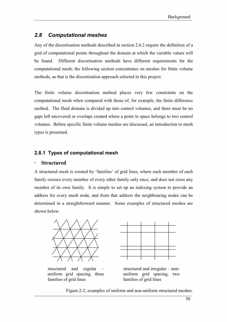
Background
50
2.8 Computational meshes
Any of the discretisation methods described in section 2.6.2 require the definition of a
grid of computational points throughout the domain at which the variable values will
be found. Different discretisation methods have different requirements for the
computational mesh; the following section concentrates on meshes for finite volume
methods, as that is the discretisation approach selected in this project.
The finite volume discretisation method places very few constraints on the
computational mesh when compared with those of, for example, the finite difference
method. The fluid domain is divided up into control volumes, and there must be no
gaps left uncovered or overlaps created where a point in space belongs to two control
volumes. Before specific finite volume meshes are discussed, an introduction to mesh
types is presented.
2.8.1 Types of computational mesh
Structured
A structured mesh is created by ‘families’ of grid lines, where each member of each
family crosses every member of every other family only once, and does not cross any
member of its own family. It is simple to set up an indexing system to provide an
address for every mesh node, and from that address the neighbouring nodes can be
determined in a straightforward manner. Some examples of structured meshes are
shown below.
Figure.2-2, examples of uniform and non-uniform structured meshes.
structured and regular –
uniform grid spacing, three
families of grid lines
structured and irregular – non-
uniform grid spacing, two
families of grid lines
Background
51
The main advantage of structured meshes is that each control volume is geometrically
similar; i.e. has the same number of sides, and neighbour finding routines are
relatively simple as the addresses of the neighbour nodes always have the same
relationship to the address of the node being considered.
A disadvantage of using structured meshes is that it quickly becomes very difficult to
mesh any but the simplest of geometries in a satisfactory manner. Curved or irregular
domain boundaries present a particular challenge. Special ‘one-off’ volumes are
created at the boundary which require special treatment during the discretisation
process. The meshing of complex geometry domains will be discussed in the next
section. Furthermore, the concentration of grid points in one particular region for
accuracy of the solution there can lead to unnecessary concentration of points in other
regions which is wasteful of computational resources.
Curvilinear structured meshes have been used extensively to study the flow around
rigid aerofoils using a geometric transformation between the curvilinear ‘real’ grid
and the Cartesian ‘computational’ grid.
Unstructured
In the most general sense, an unstructured mesh is made up nodes which can be
connected to any number of their nearest nodes. The resulting mesh polygons can
have any number of sides and the size and shape of one element will in general be
independent of that of its neighbouring elements. Some examples are shown in the
following diagram:
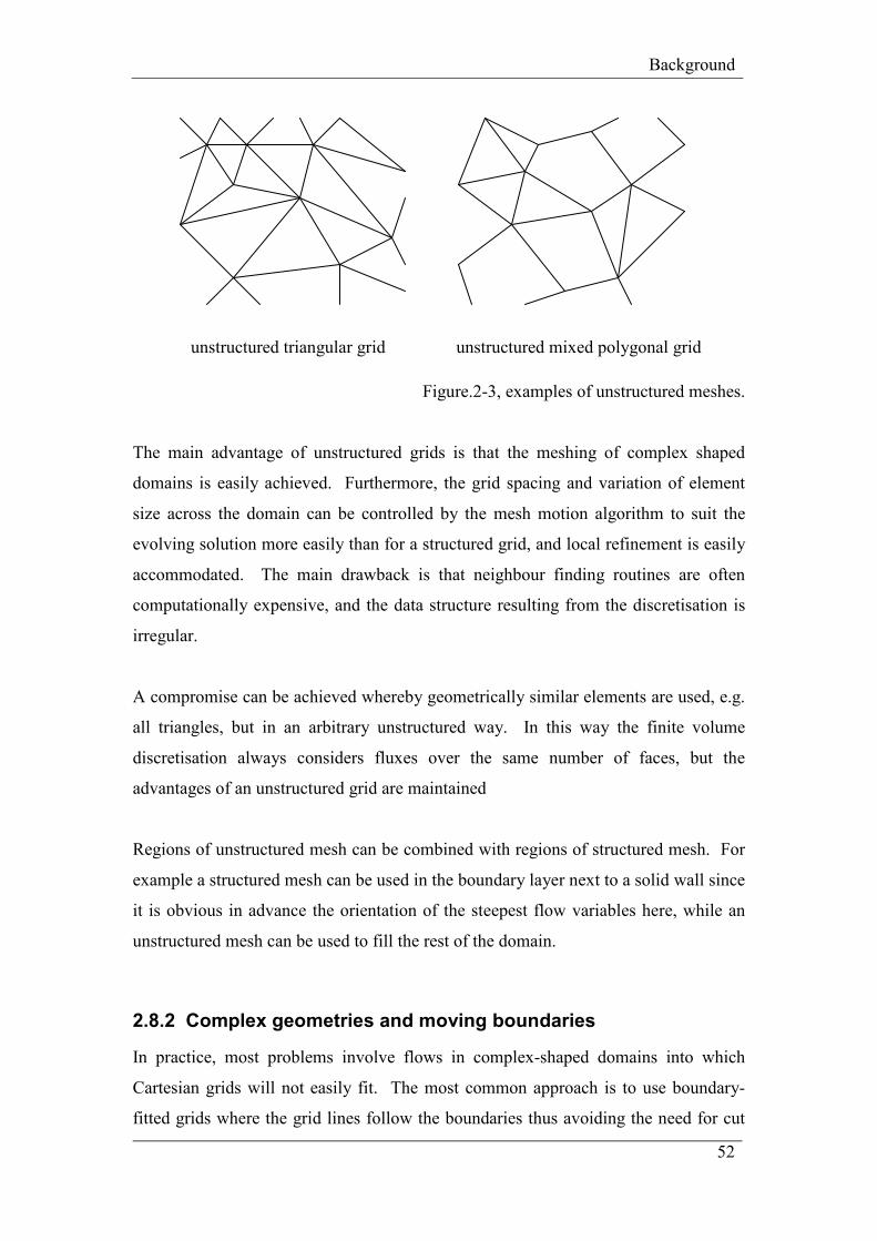
Background
52
Figure.2-3, examples of unstructured meshes.
The main advantage of unstructured grids is that the meshing of complex shaped
domains is easily achieved. Furthermore, the grid spacing and variation of element
size across the domain can be controlled by the mesh motion algorithm to suit the
evolving solution more easily than for a structured grid, and local refinement is easily
accommodated. The main drawback is that neighbour finding routines are often
computationally expensive, and the data structure resulting from the discretisation is
irregular.
A compromise can be achieved whereby geometrically similar elements are used, e.g.
all triangles, but in an arbitrary unstructured way. In this way the finite volume
discretisation always considers fluxes over the same number of faces, but the
advantages of an unstructured grid are maintained
Regions of unstructured mesh can be combined with regions of structured mesh. For
example a structured mesh can be used in the boundary layer next to a solid wall since
it is obvious in advance the orientation of the steepest flow variables here, while an
unstructured mesh can be used to fill the rest of the domain.
2.8.2 Complex geometries and moving boundaries
In practice, most problems involve flows in complex-shaped domains into which
Cartesian grids will not easily fit. The most common approach is to use boundary-
fitted grids where the grid lines follow the boundaries thus avoiding the need for cut
unstructured triangular grid unstructured mixed polygonal grid
Background
53
cells at the boundary or interface. If a structured grid is still maintained then it will in
general be non-orthogonal and have non-uniform spacings. A boundary-fitted
unstructured grid is the most flexible type to apply in this case. It is important, for
accuracy, to limit the non-uniformity of the grid so that adjacent control volumes do
not vary too greatly in size.
2D triangular or 3D tetrahedral unstructured grids are widely used for the analysis of
flow in complex domains. Delaunay triangulation techniques (Delaunay (1934)) are
popular for the initial generation of the mesh geometry and connectivity.
When the boundaries of the domain move with time, a mesh approach must be used
which ensures that the mesh remains over the entire domain. When regular structured
grids are used, the approach can be taken wherein new elements are created or old
ones discounted as the boundary moves across the domain. However, when the
geometry of the boundary is more complex, this can result in irregular shaped cut
elements as described above, or various mesh refinement techniques implemented at
the boundary.
An alternative approach is to use a mesh which maintains its topology but where the
mesh nodes move from one timestep to the next, driven by the motion of the
boundary. The total number of elements, and their topological relationships to each
other, remain constant throughout the simulation. However, the geometry of each
element will change from one timestep to the next. In particular, it is important to
note the change in volume of an element and to keep track of its aspect ratio to avoid
any elements becoming too distorted. Various mesh-moving techniques have been
developed to control the motion of the mesh nodes, and shall be discussed in chapter
6.
Literature of applications
54
3 Literature of applications
3.1 Membrane airfoils & sails
A sail can be considered as a membrane producing mainly lift at low angles of
incidence and mainly drag as a bluff body at high angles of incidence. The sail shape
is a function of the angle of incidence and the Reynolds number (usually related to the
chord length of the membrane) of the flow. The sail shape interacts strongly with the
flow, and is generally governed by the pressure distribution over both sides of the
surface.
Newman (1987) provides a summary of classical sail analysis up to that date.
Considering the two-dimensional case of a membrane held at leading and trailing
edges, static mechanics can be used to write the equations of equilibrium in terms of
pressure difference between upper and lower surfaces, tension and radius of
curvature. i.e. using static mechanics. Further, if steady inviscid and incompressible
flow and small camber and small angle of incidence is assumed the equations are
linearised and can be solved by various techniques. The variation of tension along the
membrane is neglected since skin friction is nonexistent in an inviscid flow.
Neglecting viscosity impacts on the results much more than the linearising
assumptions. Thick boundary layers and separation near leading edge are not
modelled which results in solutions for tension coefficients lower than those found
experimentally.
Further discrepancies occur when considering the modelling of luffing (the oscillation
of the sail between two equilibrium positions of opposite camber when the angle of
attack is reduced to a near zero or slightly negative value). Again this is attributed to
flow separation and thick boundary layers. The linearised model predicts that the sail
should be bistable when angle of attack is zero whereas experimental results shows
real sails can be stable for slightly negative angles of attack.
Newman lists the primary difficulties of modelling three-dimensional sails including;
non-linear elastic deformations of the sail, non-isotropic and/or non-linear material
behaviour because of the woven construction of the fabric (or due to local reinforcing
Literature of applications
55
effects), non-rigid sail boundaries (masts, ropes etc.) with respect to which the sail can
move, variation of the angle of attack with height, boundary layer separation and
reattachment which gives rise to the discrepancies between inviscid linearised models
and experimental results. In the majority of cases noted by Newman, the last two
complications are neglected.
The approach cited by Newman (1987) as the most promising method for the three-
dimensional aerodynamic analysis of membrane sails was that of Jackson & Christie
(1987) based on the fully numerical method of Jackson (1972) combining the vortex
lattice method to find the pressure distribution on the membrane, with the finite
element method of Christie (1982) for the calculation of the membrane deformations.
The authors aimed to consider the complex three-dimensional problem while avoiding
making the common simplifying assumptions of structural behaviour, in order to
capture the fully non-linear response of a flexible membrane under load.
The vortex lattice method uses inviscid flow theory, and replaces the lifting surface by
a vortex sheet lying on the surface of the wing and in its wake. The vortex lattice is
triangular in pattern, and the triangles coincide with the triangular finite elements.
The total velocity at a point is then the combination of the incident flow velocity and
the velocity induced there by the vortex loops.
The Kutta condition is satisfied at the trailing edge by shedding trailing vortices into
the flow forming a trailing vortex wake. Thus separation is assumed only to occur at
the trailing edge. Once the fluid pressure and elastic nodal force equations have been
obtained, the iterative Newton-Raphson method is used to solve for the nodal
displacements. As the method is based on inviscid flow theory, viscous drag forces
on the membrane are not accounted for and separation is not predicted. The authors
suggest that their method could be used to find the external pressure gradient, which
could then be combined with conventional boundary layer calculations for a wing of
known shape.
Having suggested the combination of inviscid flow theory corrected for viscous
effects in the first author’s 1987 paper, Jackson & Fiddes (1995) return to the two-
dimensional model and consider the formulation of a coupled viscous-inviscid
Literature of applications
56
interaction method by combining a new inviscid model with a boundary layer
calculation and coupling the resulting flow to a structural model for the membrane.
The viscous effects are considered as a leading edge separation bubble and a thin
boundary layer. The model is limited to small angles of incidence and small camber
membranes since the boundary layers downstream of the separation bubble are
assumed to remain attached.
The structural model uses a panel discretisation to describe the shape of the
membrane in finite difference form, and relate the pressure difference across the panel
and the surface shear stress to the membrane tension and the local curvature. The
iterative procedure of Jackson (1984) is used to solve for the membrane shape given a
first guess of the slope and tension of the first panel.
The overall method uses the structural iterations to find the membrane shape in
equilibrium with the inviscid flow from an initial first guess shape. The viscous
effects consisting of the leading edge separation bubble and the boundary layer
calculations then give the viscous pressure distribution, which is combined with the
initial inviscid values and the equilibrium shape is again iterated until only small
shape changes in the computed tension and lift coefficients are observed.
Further study of the behaviour of two-dimensional membrane airfoils has been carried
out by Shyy & Smith (1995) where viscous laminar flow is considered. The authors
recognise that disagreement between inviscid potential flow theory and experimental
studies is due to the presence of thick boundary layers or regions of separated flow,
particularly near the trailing edge, and that these viscous effects will be much more
influential than the effects of the assumptions made by linearised thin aerofoil theory.
Thus their aim is to produce a model capable of fully viscous flow analysis.
The Navier-Stokes equations describing unsteady laminar incompressible flow are
formulated in two-dimensional Cartesian coordinates, and then extended to general
curvilinear coordinates. A pressure based flow solver is implemented through a finite
volume formulation over a non-orthogonal body fitted grid. A staggered grid is used
for discretisation, second order upwind differencing is used in the physical
Literature of applications
57
dimensions and first order backward time differencing is implemented for the
prediction of grid velocities. The equilibrium of the membrane structure is
formulated in discrete form using the finite difference method, and relates the
curvature and tension in the membrane to the pressure difference and surface shear
forces. The length of the membrane is calculated with finite sum discretisation.
Central differencing is adopted and the finite difference equations are solved using a
line iteration method with under-relaxation.
A body fitted grid is used which is updated as the wing deforms during the course of
the aeroelastic iterations. A simple function is used which causes the influence of the
membrane motion to decay exponentially with increasing distance from the surface.
The cyclic solution of the membrane and flow equations continues iteratively until
membrane equilibrium is reached. A fully implicit time integration scheme is then
used to advance the solution to the next time step and the aeroelastic iteration is
restarted.
It was found that the algorithm could successfully demonstrate substantial changes in
membrane profile. Viscosity was shown to play a dominant role in the unsteady
membrane dynamics since the acceleration and deceleration of the free-stream
velocity strongly influenced the separation and reattachment of the flow as suggested
by the periodic appearance and collapse of recirculation zones that was observed.
Thus the aeroelastic response of the membrane was shown not to be a simple
harmonic response to the forcing frequency but a complexly coupled aerodynamic
and elastic system.
The previous algorithm is extended in a paper by Smith & Shyy (1996) to the
turbulent flow regime. The Reynolds-averaged Navier-Stokes (RANS) equations are
supplemented with the shear-stress transport (SST) k-ω model. Computations are
carried out under flow conditions similar to those for a typical marine sail and for an
inextensible membrane with no prestress. It was found that the computation time
increased substantially in cases where flow separation occurred or where the
membrane profile became inflected but overall the algorithm was stable and reliable.
Literature of applications
58
It was found that, for angles of attack outside a few degrees from zero, or for
membranes of larger excess lengths, the viscous effects dominate as shown by
observations of separation, recirculation and stagnation regions and therefore inviscid
theory-based models would fail. The RANS-based model was shown to be a viable
alternative to the classical theory but had mixed success when compared to the
experimental data. Discrepancies between the computational results and experimental
observations, and inconsistencies between different experimental reports, are
accredited to a number of physical factors; variations in Reynolds number and excess
length ratio between different authors, effect on the flow of the leading edge support
arrangement, wall effects, and non-negligible bending stiffness of the aerofoil.
Literature of applications
59
3.2 Flexible filaments & flags
The problem of a one-dimensional structure moving in a two-dimensional fluid has
recently been investigated in two papers considering the motion of flexible filaments
in flowing soap films (Farnell, David & Barton (2004a, 2004b)). In the first paper a
single filament is studied and is made to behave in either a stationary or oscillatory
stable mode by varying its length. In the second paper, a pair of filaments is
introduced to the flow, and is made to oscillate either in phase or in anti-phase by
controlling their separation distance. The experimental equivalent of this
computational experiment is presented by Zhang et al (2000).
A finite element formulation is used for the solution of the non-dimensionalised
Navier-Stokes equations, employing four-noded linear quadrilateral elements.
Velocity varies linearly between nodes, but pressure is stored at the element centre as
a piecewise discontinuous function. The code allows moving boundary constraints to
be applied within the domain to represent the position and velocity of the moving
filament. No-slip boundary conditions are applied to the sides of the domain and at
the filament surface, and inlet and outlet pressures are specified to give a satisfactory
maximum velocity.
The filament is approximated as an ‘N-tuple pendulum’ being composed of N equal
length equal mass homogeneous filament elements. Each hinge between elements has
an associated positive spring stiffness and positive damping coefficient. Lagrangian
mechanics formulation is used to assemble equations for the kinetic energy and for
the potential energy of the filament in terms of the hinge rotations. The fluid pressure
is converted into an external force on the pendulum by considering it to be constant
along the length of a given filament element. Solution of the Euler-Lagrange
equations for the angular accelerations is carried out numerically (e.g. LU
decomposition). The angular accelerations and velocities are then used to predict the
angular velocities and displacements at the next time step using Runge-Kutta
integration, from which the next angular accelerations can again be found.
The filament is mapped onto the CFD mesh as follows. The filament is given a finite
width, centred about the filament centre line. CFD nodes lying within this strip are
Literature of applications
60
identified as boundary nodes and are assigned the velocity of the nearest filament
element centre, thus enforcing the no-slip condition. After solution of the Navier-
Stokes equations over the next small time increment, the fluid pressures are mapped
back onto the element as follows. The fluid pressure is sampled at all nodes lying
within a fixed distance (twice the filament thickness) of the filament surface, but not
within the filament. These values are then averaged over the element and the
resulting forces are input into the formulation of the Euler-Lagrange equations. From
this the position of the filament is updated and the process is repeated for a
predetermined number of time steps.
A stable oscillatory state was achieved, with amplitude of oscillation larger than the
initial angles indicating that the filament had drawn energy from the flow. The bluff
body shape of the leading edge was seen to induce boundary layer separation as
expected and two small recirculation zones were created. However, as the filament is
deformable, these were not shed in the normal manner, but were enhanced and grown
by the curvature of the filament as they were convected downstream and subsequently
shed from the trailing edge. The curvature of the filament is a result of the vortex
itself, demonstrating the complex behaviour in this relatively simple system.
Literature of applications
61
3.3 Parachutes and airbags
The modelling of the descent of payloads under parachutes, or of the interaction of
parachutes with the wake of an aircraft presents similar challenges to the modelling of
tensile fabric structures in wind. The primary difference is that the stability of the
parachute surface is imparted only through the aerodynamic effects – i.e. there is no
prestress to be taken into account.
In a series of papers, Stein, Tezduyar and co-workers study various problems
involving the modelling of parachute canopies and the surrounding airflow. In Stein
et al (2001) a model is developed to study the unsteady descent of a round parachute,
including the modelling of turbulent flow effects. Tezduyar & Osawa (2001b)
consider the interactions of a parachute canopy passing through the far wake of an
aircraft, and Stein et al (2004) study the simulation of the ‘soft’ landing of clusters of
cargo parachutes.
All three papers make use of the Deforming-Spatial-Domain / Stabilised-Space-Time
(DSD/SST) finite element approach of Tezduyar (1991) and Tezduyar, Behr & Liou
(1992). This approach makes use of finite element interpolation functions which are
functions of both space and time. The time step is divided into a number of discrete
time slabs, and the method updates the position of the domain boundaries at each
iteration as part of the solution. The movement of the domain boundaries is thus
taken into account automatically. The approach has previously been applied to
problems involving moving cylinders and aerofoils, flow in flexible pipes and two-
phase fluid-structure interaction problems.
Central to the DSD/SST approach is the Streamline Upwind/Petrov-Galerkin (SUPG)
interpolation technique of Brooks & Hughes (1982), and the Pressure-
Stabilising/Petrov-Galerkin (PSPG) technique of Tezduyar (1991), which help to
ensure numerical stability of the scheme while allowing equal order interpolation
functions for both velocity and pressure. The SUPG and PSPG techniques prevent
numerical oscillations occurring in flows of high Reynolds number or in boundary
layers. The DSD/SST approach has been validated against wind tunnel tests for the
Literature of applications
62
steady-state case of a fully inflated parachute in a uniform freestream flow field Stein
et al (1999).
The DSD/SST finite element approach is used to discretise the incompressible
Navier-Stokes equations. Stein et al (2001) also include the Smagorinsky zero-
equation turbulence model. The structural dynamics model makes use of the
momentum balance membrane equations assuming large displacements and rotations
but small strains of a linear elastic Hookean material. The finite element
discretisation makes use of plane stress triangular elements, and follows the virtual
work approach. Cables are modelled as uniaxial tension elements. The canopy mesh
is then used to generate a 3D unstructured tetrahedral fluid mesh.
The prestress shape of the canopy is found by solving the structural system under an
applied uniform pressure differential. This canopy shape is then held fixed whilst a
number of flow calculations are carried out to establish developed flow around the
canopy. The shape of the canopy at this point does not necessarily correspond to the
fluid forces exerted on it. A number of fluid-structure calculations are carried out
with the parachute payload held in place, so that the canopy shape and flow field can
converge on a steady equilibrium position. All nodes on the structure model can then
be freed and the acceleration towards terminal descent proceeds.
When considering the interactions of the parachute with the far wake of an aircraft
(Tezduyar & Osawa (2001b)), the authors make use of the multi-domain method of
Tezduyar & Osawa (1999). The fluid domain is divided into a number of
subdomains, the object creating the wake is placed in the first subdomain, and then a
number of subdomains follow downstream. The inflow conditions on each
subdomain are extracted from the flow solution of the subdomain immediately
upstream. This model was used in Tezduyar & Osawa (2001a) to calculate the wake
data and its interaction with a rigid parachute canopy. A further subdomain surrounds
the parachute canopy and payload, and follows it as it moves across the main fluid
domain. The boundary conditions for the parachute subdomain are extracted from the
flow solution in the main flow domain at the relevant locations at that particular
instant in time.
Literature of applications
63
The aims of the mesh moving algorithm are to minimise frequency of remeshing of
the domain, since this procedure is computationally expensive and introduces errors
into the solution when the flow variables are projected from the old mesh onto the
new mesh. The constraint on the mesh motion algorithm is that, at the interface, the
normal mesh velocity must be equal to the normal fluid velocity. The mesh motion
follows the pseudosolid approach, whereby the displacements of the mesh nodes are
calculated treating the mesh as a linear elastic solid with imposed boundary
deformations given by the canopy shape. Stiffnesses are assigned to the mesh
elements such that the smaller elements deform less and move more like rigid bodies,
whereas larger elements undergo more deformation. Since the parachute movements
are unpredictable, this approach is preferable to a purely algebraic approach which
has been applied in the past. This mesh moving approach, however, is not capable of
handling structure-structure contact, so if this occurs the simulations are halted.
A block iterative coupling approach is used; the fluid, structure and mesh systems are
solved in turn, using the latest available values of all other variables at each stage.
Stein et al (2004) find that it is difficult to converge this loose coupling approach
successfully. They claim that this is due to the high flexibility of the structure which
means that the structural response is very sensitive to changes in the flow solution.
They apply an artificial increase to the inertia terms of the structural dynamics
equations to damp the response of the structure. The applied forces remain
unchanged so the structure system still converges on the correct form. In the cases
where incompatible structure and fluid meshes are used, a least squares projection
method is used to transfer the information.
When considering the inflation behaviour of an airbag, Mestreau & Lohner (1996)
combine commercial fluids and structure finite element codes in a loose coupled
approach. Both codes are widely used and verified for crashworthiness testing, and
the loose coupling approach allows for minimum alteration of the existing modules.
Previous work has studied the inflation behaviour of an airbag under a uniform
pressure differential, but in this paper the authors hope to model the effects of the
airstream jet visible in the early stages of inflation, since experimental investigation
has shown that this jet is responsible for the majority of injuries to drivers seated too
close to the airbag.
Literature of applications
64
The simulation neglects viscous effects so the fluid system is based on the Euler
equations. At the fluid structure interface, normal velocities of fluid and structure are
equal, but tangentially the systems are allowed to slip relative to each other. The fluid
mesh is made up of tetrahedra, and the algorithm monitors mesh quality and carries
out re-meshing, by the advancing front method, as necessary based on element aspect
ratio. Transfer of information at the interface is carried out in a conservative manner
using integral techniques, although no details are given.
Literature of applications
65
3.4 Tensile fabric structures
In order to study a fully three-dimensional fluid structure interaction problem, Glück
et al (2001) undertake the coupling of two highly developed computer analysis codes
through the implementation of a coupling interface to manage the exchange of data
between the two codes.
The CFD code is a finite volume based solver for the incompressible Reynolds-
averaged Navier-Stokes (RANS) equations, operating over a non-staggered block
structured hexahedral grid. The k-ε turbulence model is included for closure. The
space conservation law is fulfilled and the Arbitrary Lagrangian Eulerian (ALE)
formulation for flows over moving grids is implemented. Discretisation in time is by
fully implicit second order accurate methods, while spatial discretisation uses upwind
differencing, central differencing or a combination, based on a deferred correction
approach.
The structural dynamics code considers the equations of motion of the structure as a
thin-walled reduced model. A finite element formulation is carried out over a
quadrilateral mesh. A linear acceleration of the structure is assumed within each
time-step, and non-linear effects such as large displacements or material properties are
taken into account by means of a Newton-Raphson approach within each time-step.
As the CFD domain contains many more grid points than those used for the structure
calculation, multiple processors were employed based on a domain decomposition
approach. A neutral geometric model was used to support the exchange of variables
between the two grids. As not all grid nodes were coincident, some interpolation was
necessary. To transfer pressure and shear onto the structural grid, the conservative
interpolation of Farhat, Lesionne & LeTallec (1998) was used, which ensures that the
load resultants are the same on each grid. To transfer the displacement vectors onto
the fluid mesh, a bilinear interpolation was used which is consistent with the shape
functions used in the finite element formulation.
A predictor-corrector scheme was also used to reduce the number of iterations needed
for convergence. The boundary geometry from the last three time-steps was used to
Literature of applications
66
predict the geometry for the next time step; a scheme which has second order
accuracy in time. Algebraic methods were used for grid adaptation, such as linear
interpolation within blocks, transfinite interpolation and problem-adapted higher-
order polynomials to generate the block faces near the distorted structure.
The final test case is the fully three-dimensional analysis of a membrane roof
structure to find the steady state deformations. The starting geometry of the
membrane is found using form finding after Bellman (1998) based on the prestress
state and mass of the fabric. The structural dynamics computations used membrane
elements unable to resist bending forces. The wind load was a steady inlet velocity of
30 m/s corresponding to a Reynolds number of 6x10⁶ and the wind pressure forces
and structure displacements were produced.
In their second paper Glück et al (2003), the authors use the same coupled fluid-
structure techniques (although without turbulence modelling) to study the dynamic
time-dependent behaviour of the tent roof after the application of a wind gust over the
basic flow. Laminar flow regime was assumed, with a Reynolds number of 120 based
on the leading edge dimension of the roof and the maximum gust velocity of 40m/s.
The gust followed a Gaussian curve in both time and space and was superimposed
over a basic wind speed of 10m/s at a height of 10m above the ground.
An extension of the technique for the study of time-dependent structural motion under
turbulent flow is recommended through the use of Large Eddy Simulation since time-
dependent turbulent flows cannot be solved satisfactorily because of weaknesses of
the k-ε type turbulence models. The modelling of turbulent flow is necessary to study
flows of practical civil engineering interest. In both papers the authors explain that
comparison between their numerical data with experimental observation is not
possible due to a great lack of experiments in the area.
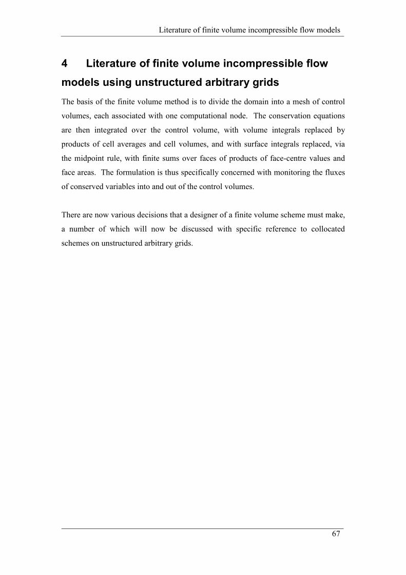
Literature of finite volume incompressible flow models
67
4 Literature of finite volume incompressible flow
models using unstructured arbitrary grids
The basis of the finite volume method is to divide the domain into a mesh of control
volumes, each associated with one computational node. The conservation equations
are then integrated over the control volume, with volume integrals replaced by
products of cell averages and cell volumes, and with surface integrals replaced, via
the midpoint rule, with finite sums over faces of products of face-centre values and
face areas. The formulation is thus specifically concerned with monitoring the fluxes
of conserved variables into and out of the control volumes.
There are now various decisions that a designer of a finite volume scheme must make,
a number of which will now be discussed with specific reference to collocated
schemes on unstructured arbitrary grids.
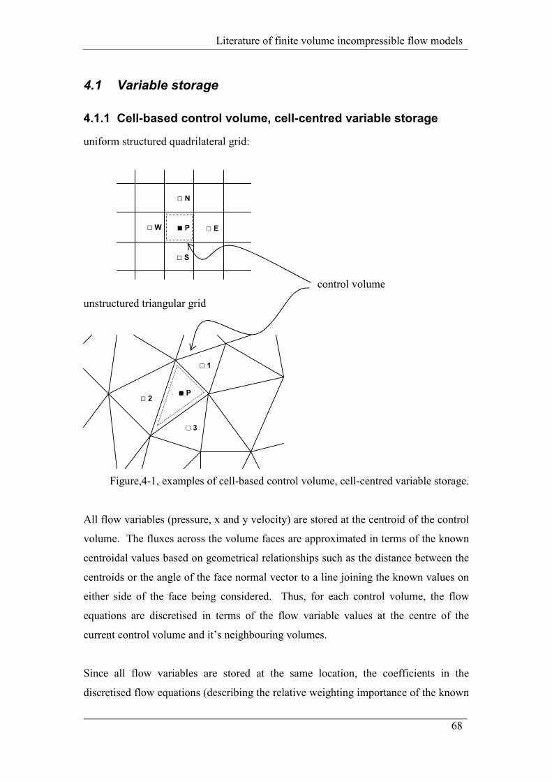
Literature of finite volume incompressible flow models
68
4.1 Variable storage
4.1.1 Cell-based control volume, cell-centred variable storage
uniform structured quadrilateral grid:
control volume
unstructured triangular grid
Figure,4-1, examples of cell-based control volume, cell-centred variable storage.
All flow variables (pressure, x and y velocity) are stored at the centroid of the control
volume. The fluxes across the volume faces are approximated in terms of the known
centroidal values based on geometrical relationships such as the distance between the
centroids or the angle of the face normal vector to a line joining the known values on
either side of the face being considered. Thus, for each control volume, the flow
equations are discretised in terms of the flow variable values at the centre of the
current control volume and it’s neighbouring volumes.
Since all flow variables are stored at the same location, the coefficients in the
discretised flow equations (describing the relative weighting importance of the known
P E
S
W
N
P
1
3
2
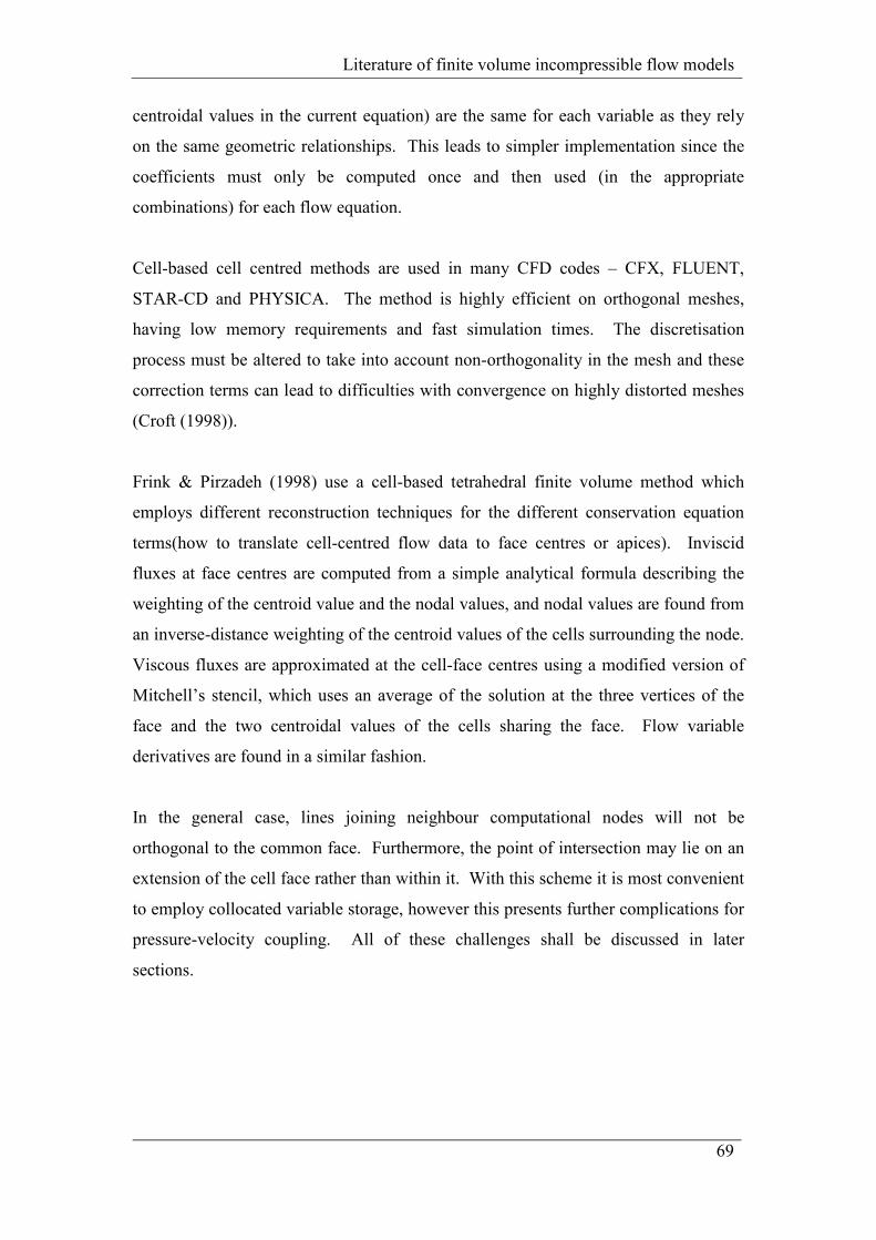
Literature of finite volume incompressible flow models
69
centroidal values in the current equation) are the same for each variable as they rely
on the same geometric relationships. This leads to simpler implementation since the
coefficients must only be computed once and then used (in the appropriate
combinations) for each flow equation.
Cell-based cell centred methods are used in many CFD codes – CFX, FLUENT,
STAR-CD and PHYSICA. The method is highly efficient on orthogonal meshes,
having low memory requirements and fast simulation times. The discretisation
process must be altered to take into account non-orthogonality in the mesh and these
correction terms can lead to difficulties with convergence on highly distorted meshes
(Croft (1998)).
Frink & Pirzadeh (1998) use a cell-based tetrahedral finite volume method which
employs different reconstruction techniques for the different conservation equation
terms(how to translate cell-centred flow data to face centres or apices). Inviscid
fluxes at face centres are computed from a simple analytical formula describing the
weighting of the centroid value and the nodal values, and nodal values are found from
an inverse-distance weighting of the centroid values of the cells surrounding the node.
Viscous fluxes are approximated at the cell-face centres using a modified version of
Mitchell’s stencil, which uses an average of the solution at the three vertices of the
face and the two centroidal values of the cells sharing the face. Flow variable
derivatives are found in a similar fashion.
In the general case, lines joining neighbour computational nodes will not be
orthogonal to the common face. Furthermore, the point of intersection may lie on an
extension of the cell face rather than within it. With this scheme it is most convenient
to employ collocated variable storage, however this presents further complications for
pressure-velocity coupling. All of these challenges shall be discussed in later
sections.
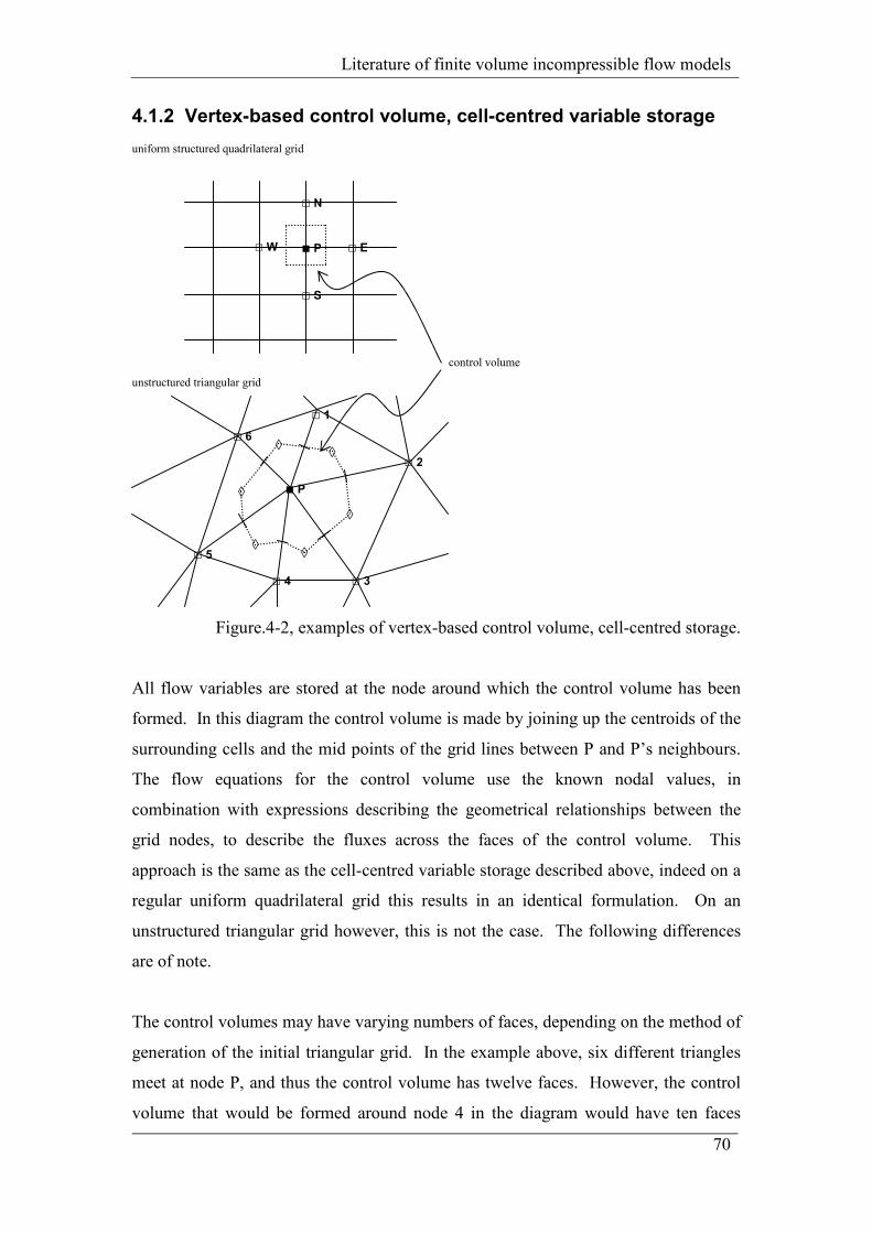
Literature of finite volume incompressible flow models
70
4.1.2 Vertex-based control volume, cell-centred variable storage
uniform structured quadrilateral grid
control volume
unstructured triangular grid
Figure.4-2, examples of vertex-based control volume, cell-centred storage.
All flow variables are stored at the node around which the control volume has been
formed. In this diagram the control volume is made by joining up the centroids of the
surrounding cells and the mid points of the grid lines between P and P’s neighbours.
The flow equations for the control volume use the known nodal values, in
combination with expressions describing the geometrical relationships between the
grid nodes, to describe the fluxes across the faces of the control volume. This
approach is the same as the cell-centred variable storage described above, indeed on a
regular uniform quadrilateral grid this results in an identical formulation. On an
unstructured triangular grid however, this is not the case. The following differences
are of note.
The control volumes may have varying numbers of faces, depending on the method of
generation of the initial triangular grid. In the example above, six different triangles
meet at node P, and thus the control volume has twelve faces. However, the control
volume that would be formed around node 4 in the diagram would have ten faces
P
N
E
S
W
◊
◊ ◊
◊
◊ ◊
1
3 4
5
6
2
P
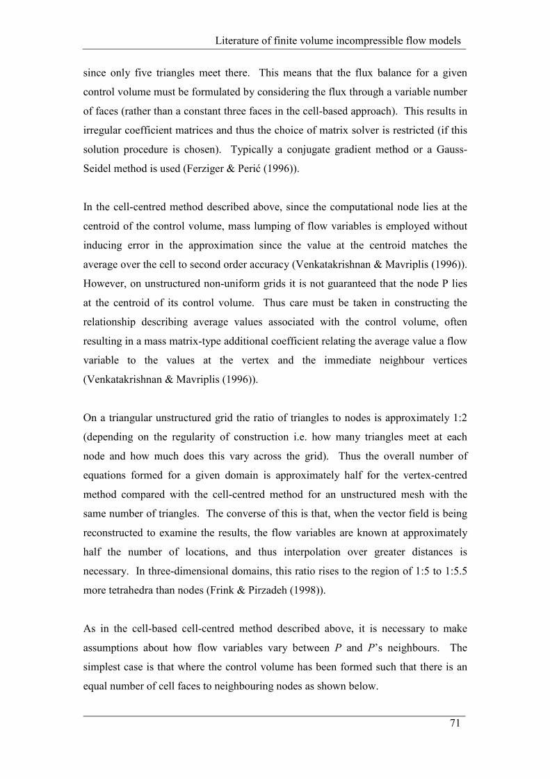
Literature of finite volume incompressible flow models
71
since only five triangles meet there. This means that the flux balance for a given
control volume must be formulated by considering the flux through a variable number
of faces (rather than a constant three faces in the cell-based approach). This results in
irregular coefficient matrices and thus the choice of matrix solver is restricted (if this
solution procedure is chosen). Typically a conjugate gradient method or a Gauss-
Seidel method is used (Ferziger & Perić (1996)).
In the cell-centred method described above, since the computational node lies at the
centroid of the control volume, mass lumping of flow variables is employed without
inducing error in the approximation since the value at the centroid matches the
average over the cell to second order accuracy (Venkatakrishnan & Mavriplis (1996)).
However, on unstructured non-uniform grids it is not guaranteed that the node P lies
at the centroid of its control volume. Thus care must be taken in constructing the
relationship describing average values associated with the control volume, often
resulting in a mass matrix-type additional coefficient relating the average value a flow
variable to the values at the vertex and the immediate neighbour vertices
(Venkatakrishnan & Mavriplis (1996)).
On a triangular unstructured grid the ratio of triangles to nodes is approximately 1:2
(depending on the regularity of construction i.e. how many triangles meet at each
node and how much does this vary across the grid). Thus the overall number of
equations formed for a given domain is approximately half for the vertex-centred
method compared with the cell-centred method for an unstructured mesh with the
same number of triangles. The converse of this is that, when the vector field is being
reconstructed to examine the results, the flow variables are known at approximately
half the number of locations, and thus interpolation over greater distances is
necessary. In three-dimensional domains, this ratio rises to the region of 1:5 to 1:5.5
more tetrahedra than nodes (Frink & Pirzadeh (1998)).
As in the cell-based cell-centred method described above, it is necessary to make
assumptions about how flow variables vary between P and P’s neighbours. The
simplest case is that where the control volume has been formed such that there is an
equal number of cell faces to neighbouring nodes as shown below.
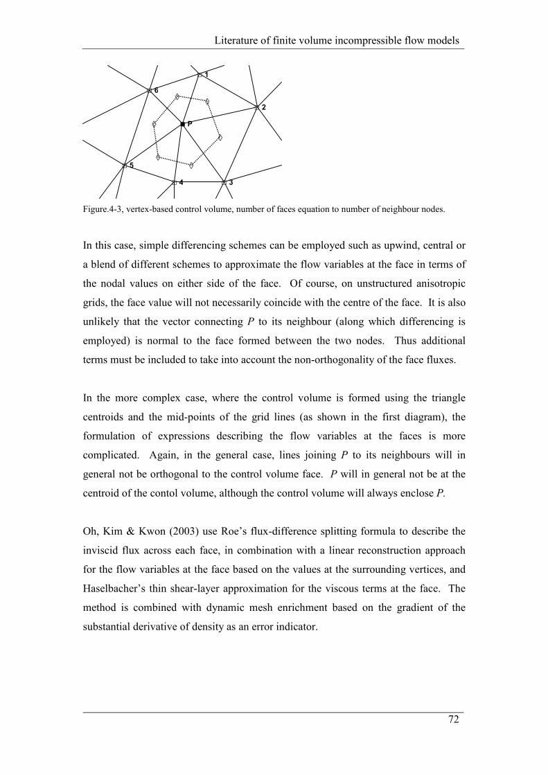
Literature of finite volume incompressible flow models
72
Figure.4-3, vertex-based control volume, number of faces equation to number of neighbour nodes.
In this case, simple differencing schemes can be employed such as upwind, central or
a blend of different schemes to approximate the flow variables at the face in terms of
the nodal values on either side of the face. Of course, on unstructured anisotropic
grids, the face value will not necessarily coincide with the centre of the face. It is also
unlikely that the vector connecting P to its neighbour (along which differencing is
employed) is normal to the face formed between the two nodes. Thus additional
terms must be included to take into account the non-orthogonality of the face fluxes.
In the more complex case, where the control volume is formed using the triangle
centroids and the mid-points of the grid lines (as shown in the first diagram), the
formulation of expressions describing the flow variables at the faces is more
complicated. Again, in the general case, lines joining P to its neighbours will in
general not be orthogonal to the control volume face. P will in general not be at the
centroid of the contol volume, although the control volume will always enclose P.
Oh, Kim & Kwon (2003) use Roe’s flux-difference splitting formula to describe the
inviscid flux across each face, in combination with a linear reconstruction approach
for the flow variables at the face based on the values at the surrounding vertices, and
Haselbacher’s thin shear-layer approximation for the viscous terms at the face. The
method is combined with dynamic mesh enrichment based on the gradient of the
substantial derivative of density as an error indicator.
◊
◊ ◊
◊ ◊
◊
2
3 4
1
6
5
P
Literature of finite volume incompressible flow models
73
Alternatively, the flow variables can be represented by piecewise algebraic
expressions, the simplest being that the variables vary linearly within each triangle
according to:
cbyax ++=φ [4.1],
where a, b and c can be found using the three nodal values of the triangle concerned.
The finite volume formulation for the control volume can then proceed, with the
contributions of each face being evaluated by the contribution of each subvolume,
within which an algebraic expression for the flow variables is known and can thus be
easily differentiated to find variable gradients or integrated over the face area.
subvolume,
φ bilinear between P, 2 and 3.
Figure.4-4, vertex-based control volume with bilinear subvolumes.
This approach, using element piecewise linear shape functions, has been shown to
handle distorted meshes with relative ease but is computationally expensive.
Combinations of cell-based cell-centred and vertex-based cell-centred methods can be
used, for example where the flow solution is found using the vertex-based control
volumes, and other transported variables are solved using cell-based control volumes.
Thus the momentum and continuity equations are discretised over a control volume
assembled around a particular grid node as described in this section, and equations
describing heat transfer and turbulence models are discretised over the mesh elements
themselves. McBride, Croft & Cross (2003) use such an approach to allow flow
solutions on highly distorted meshes while minimising the additional computational
disruption to well established cell-based code. The vertex-based variables are
◊
◊ ◊
◊ ◊
◊
2
3 4
1
6
5
P
Literature of finite volume incompressible flow models
74
approximated using linear element piecewise functions. They find that the time per
iteration per solution point for the vertex-based variables was approximately four
times greater than that for the cell-based variables and the memory requirements
approximately eight times greater, but that it was possible to resolve the flow field on
highly distorted grids which otherwise caused divergence of the solution when using a
purely cell-based approach.
Date (2005) describes the circum-centre approach, where the computational node is
set at the circum-centre of the triangle. The advantage of this approach is that the
lines joining neighbour nodes are always orthogonal to the common cell face,
however there is no guarantee that the circum-centre will lie within the control
volume. This scheme is easily extended to three dimensions by considering the
circum-sphere of a tetrahedral element.
Literature of finite volume incompressible flow models
75
4.2 Interpolation & stability
After discretisation of the conservation equations following the finite volume method,
the equations require the values of the unknown flow variables at the cell faces in
order to evaluate the face fluxes. These face values must be written in terms of the
variable values at the computational nodes.
The simplest approach is to use a linear interpolation between the two nodes
straddling the face based on the distance of the node from the face. However, this can
introduce instabilities in cases where the flow is dominated by convective effects. In
these cases, it is common to introduce a degree of ‘upwinding’ into the differencing
scheme. This is where the computational node on the upwind side of the face being
considered contributes relatively more importantly to the resulting face value than that
on the downwind side.
Hybrid differencing involves a using a choice between central differencing and
upwind differencing according to the cell Peclet number (which describes the ratio
between the cell dimensions and the local fluid velocity). These schemes can take the
form of a deferred correction approach, where a blend is made between implicit
central differencing and explicit upwind differencing, in order to simplify the
resulting equations. Demirdzic & Peric (1990) use this approach, and have found that
the effective added numerical diffusion has the effect of increasing the diagonal
dominance of the equation set which aids stability and helps to damp out oscillations
in the solution. On a structured grid, the quadratic upwind differencing scheme of
Leonard (1979) is often used which involves fitting a quadratic curve to the two
upwind and one downwind computational nodes around the face.
Various other curve fitting or hybrid differencing schemes have been proposed, but
often are not applicable to arbitrary unstructured grids since it cannot always be
guaranteed that the closest nodes to the face exist in the direction required in order to
reconstruct the variable profile.
Davidson (1996) finds that an additional 4th order dissipation term is required for
stability when interpolating convective velocities for the test case of a backward
Literature of finite volume incompressible flow models
76
facing step but not for the case of a diverging channel of a skewed driven cavity.
Oscillations in the pressure field are also found at the interface between regions of the
domain where large differences in cell sizes are found, or where highly distorted cells
are used. He suggests the reconstruction schemes of Pan & Cheng (1993) and Barth
& Jespersen (1989) as useful alternative approaches. A reconstruction scheme is used
to find the variable gradients at the cell centre, and then Taylor series expansions are
used to find the variable values at the faces of the cells. This approach makes no
assumptions about the locations of the nodes used to reconstruct the gradients, and is
therefore particularly applicable to unstructured arbitrary grids.
Literature of finite volume incompressible flow models
77
4.3 Pressure-velocity decoupling
Since it is pressure gradients which drive flow, rather than overall pressure values, it
is possible to arrive at the situation where the interpolation method used to find
pressure values at the cell faces produces a discretised expression for velocity in a cell
which is independent of the value of pressure in the cell. This is effectively a
decoupling of the equations, and has the effect that the pressure is sampled from two
independent coarser grids than the velocity. Effectively the equation for velocity at a
point will feel a uniform pressure field regardless of the values of pressure involved –
a checkerboard pressure field is felt like a uniform pressure field. A number of
approaches have been developed to avoid this decoupling, and it’s destabilising
effects, from occurring.
4.3.1 Staggered grids
In the staggered grid approach, a different control volume is used when considering
the conservation of each independent variable. This has the effect that each velocity
control volume has face centre nodes coincident with the computational node at which
pressure is evaluated, and the pressure control volume faces are coincident with the
velocity computational nodes. Thus the need for interpolation to the cell faces is
avoided.
The main advantage of this approach is that terms can be evaluated to 2nd order
approximation without the need for interpolation, and a strong coupling between
velocity and pressure unknowns is achieved which avoids some types of convergence
problems and oscillations in the solution fields. However, the approach is difficult to
apply to arbitrary unstructured grids, where it is not immediately obvious what the
form and location of the related grids should be, or if the related nodes would fall at
the cell face centres on the other grids. The generation of numerical meshes is also
computationally expensive, and this approach requires the generation and
maintenance of three grids in two-dimensional studies, and four in three.
The alternative to the staggered approach which is most often applied to cases using
arbitrary unstructured grids is the collocated scheme. In this approach, one set of
Literature of finite volume incompressible flow models
78
control volumes is used and all variables are stored at same computational node at the
centre of the control volume. The advantages of the collocated approach is that the
resulting equations for each variable contain many similar terms; the geometrical
relationships of one cell to it’s neighbour are identical regardless of which variable is
being considered. This is a particular advantage where a more complex higher order
differencing scheme is being used. Computational time and storage is thus reduced.
The application of boundary conditions is also simplified, since the control volume
faces will always coincide with the domain boundary, and the condition can be
applied directly when evaluating the flux at that face. In the staggered approach half-
cells occur at the boundary for some flow variables which then require special
treatment. The collocated approach is also more suited to combination with multigrid
techniques since the same restriction and prolongation operations for transfer of
variable values are used for all variables. The main advantage remains the simplicity
of application to arbitrary non-orthogonal grids when compared to the staggered
variable storage schemes.
Peric, Kessler & Scheuerer (1988) provide a comparison of collocated and staggered
approaches on rectilinear orthogonal grids (since the staggered approach is not easily
extended to non-orthogonal grids, such a comparison is not easy). For both
approaches they find that convergence is primarily governed by the relaxation factor
applied to the velocity update, and conclude, therefore that the collocated arrangement
holds no computational disadvantage to the staggered approach, and that it’s main
advantage is it’s ease of application to arbitrary unstructured grids. The main
disadvantage is the need for special interpolation approaches to avoid the velocity-
pressure decoupling described above.
Further authors using staggered grids include Maliska & Raithby (1984), Demirdzic et
al (1987), Karki & Patankar (1989).
Literature of finite volume incompressible flow models
79
4.3.2 Higher accuracy of pressure gradient derivation
An alternative approach to avoid velocity-pressure decoupling is to retain the
colocated variable approach and devise a higher order method for the interpolation of
pressure to the cell faces or of reconstruction of pressure gradients.
Rhie & Chow (1983) present an approach which introduces a pressure smoothing
term, which is like a higher order gradient term considering the variation of the
derivative, used when finding face velocities. The approach uses a combination of
linear interpolation from straddling nodal values, with direct reconstruction of
pressure gradients. The additional pressure derivative term is used when calculating
the face normal velocities.
Melaaen (1992) finds the non-staggered approach superior to the staggered approach
on distorted grids, while other aurthors using a collocated approach include Rhie,
Delaney & McKain (1984), and Majumdar, Rodi & Zhu (1992).
Literature of finite volume incompressible flow models
80
4.4 Unstructured non-orthogonal grids
Arbitrary unstructured grids are the most convenient way to mesh a complex-shaped
domain. It is also simple to implement local grid adaptation or refinement since a cell
can have an arbitrary number of faces. The grid is arbitrary in the sense that each
node defining the mesh is connected to any number of other mesh nodes, and they are
unstructured since they are not made up of intersecting sets of grid lines. In general
the mesh elements can be any polygonal (in two dimensions) or polyhedral (in three
dimensions) shape; triangular meshes are the most common and sometimes a mixture
of triangular and quadrilateral elements is used.
The finite volume method is particularly suited to application over an arbitrary
unstructured grid since the conservation equations are formulated in terms of fluxes
over the control volume faces – there is no need to know in advance the particular
shape of the control volume. This means that the finite volume method does not need
to be restricted to a particular shape of mesh element. The only requirements on the
mesh are that it fills the whole domain with no overlaps or gaps, and that each control
volume is associated with one computational node.
Some authors (Davidson (1996), Holmes & Connel (1989)) describe the combination
of areas of structured grid in the near wall region with areas of unstructured grid in the
rest of the domain. In this way, it can be easier to guarantee that computational nodes
lie in areas of specific interest (e.g. due to high variable gradients).
However, there are a number of geometrical aspects of arbitrary unstructured grids
which require special attention during the formulation of the conservation equations.
The discretisation of the conservation equations involves the approximation of surface
integrals by applying the midpoint rule to each face of the volume. The midpoint rule
is second order accurate when the sampling point is at the centre of the face.
However, the midpoint rule reduces in accuracy to first order accurate as the sampling
point approaches one end of the face. On a general arbitrary unstructured grid there is
no guarantee that the line connecting the nodes either side of a face bisects that face.
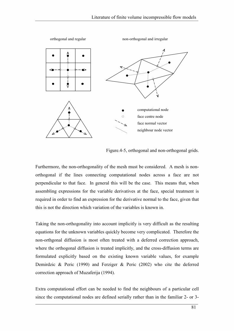
Literature of finite volume incompressible flow models
81
Figure.4-5, orthogonal and non-orthogonal grids.
Furthermore, the non-orthogonality of the mesh must be considered. A mesh is non-
orthogonal if the lines connecting computational nodes across a face are not
perpendicular to that face. In general this will be the case. This means that, when
assembling expressions for the variable derivatives at the face, special treatment is
required in order to find an expression for the derivative normal to the face, given that
this is not the direction which variation of the variables is known in.
Taking the non-orthogonality into account implicitly is very difficult as the resulting
equations for the unknown variables quickly become very complicated. Therefore the
non-orthgonal diffusion is most often treated with a deferred correction approach,
where the orthogonal diffusion is treated implicitly, and the cross-diffusion terms are
formulated explicitly based on the existing known variable values, for example
Demirdzic & Peric (1990) and Ferziger & Peric (2002) who cite the deferred
correction approach of Muzaferija (1994).
Extra computational effort can be needed to find the neighbours of a particular cell
since the computational nodes are defined serially rather than in the familiar 2- or 3-
computational node
face centre node
face normal vector
neighbour node vector
orthogonal and regular non-orthogonal and irregular
Literature of finite volume incompressible flow models
82
dimensional indexing arrangement that occurs with structured (Cartesian or
curvilinear) intersecting grid lines. If the topology of the mesh remains constant
throughout the simulation then the neighbours of one cell will remain the same,
however, if grid refinement is used then further neighbour finding routines will be
required. Indeed Taniguchi & Kobayashi (1991), when using Voronoi meshes claim
that the slower performance experienced when compared to regular structured grid is
due to the time taken to look up values in list-vectors. The advantage of using
Voronoi meshes is that the faces of the control volumes are perpendicular bisectors of
the lines connecting the computational nodes, which avoids the complications of
using arbitrary unstructured grids previously explained.
Perez-Segarra, Oliva & Consul (1996), when considering convergence properties of
various finite volume schemes, find that convergence is strongly influenced by grid
properties. When using significantly non-orthogonal grids a smaller timestep and/or
relaxation factors are required for stability which leads to slower convergence.
A further advantage of using arbitrary polygonal meshes is demonstrated by Chow,
Cross & Pericleous (1996) who compare results for regular triangular, hexagon-based
and octagon-based meshes. They find an improved accuracy using polygonal meshes
over rectangular meshes and explain that this is probably due to the fact that each cell
has a greater connectivity to its neighbour cells. In this way the arbitrary polygonal
mesh could be viewed as a higher order scheme since it uses more neighbouring node
information in the formulation of the conservation equations at a particular node.
Literature of approaches to coupling and interfacing
83
5 Literature of approaches to coupling and
interfacing
The computation of aeroelastic phenomena requires the numerical modelling of both
the fluid flow and the structure motion in order to examine the interactions between
the two systems. Furthermore, the numerical model must provide an effective means
of representing the coupled nature of the problem. A number of issues related to
modelling this coupled interacting system will now be discussed.
Literature of approaches to coupling and interfacing
84
5.1 Comparison of the behaviour of the two systems
When considering the behaviour of elastic structures, St Venant’s principle states that
small local disturbances in the stress state have only local effects on the overall stress
state of the structure. For example, the exact manner in which the tip of a cantilever
is loaded (on the top, from the bottom or distributed over the cross section) does not
influence the global behaviour but only alters the stress state in the region near to the
load point. This does not hold when considering the behaviour of a fluid; in this case
small local disturbances can have far reaching effects and the effects both in time and
space. For example, if an object is temporarily dipped into a flow stream the
behaviour of the fluid, particularly in the downstream direction, will be altered
considerably.
The implications of this difference on the design of a coupled fluid-structure model
must be considered. The effects of approximations in the structural model are quite
localised, disturbances, which could be errors in the model e.g. errors due to
discretisation method, can affect the fluid solution greatly while the structure solution
would be largely unaffected.
The convention in analysis of elastic structures is to use a Lagrangian approach, i.e.
one where a particular element contains the same particles of structure from one
timestep to the next. The numerical grid moves with the structure as it displaces and
deforms. This approach is clearly not appropriate for analysis of fluids except in the
simplest of steady laminar cases. The particle method approach described earlier is a
Lagrangian formulation, but is a mesh-less method hence grid tangling is not a
problem. A Eulerian approach is therefore adopted; in this case the fluid particles
move through the mesh from one timestep to the next. The mesh is not necessarily
stationary; its movement can be governed by other requirements of the model such as
moving boundaries. A result of this is that the two systems of equations of motion
describing the different fields behave very differently. the structure system is stiffer
than the fluids system. This means that if a direct solution technique is to be used i.e.
matrix inversion, then the choice of solvers which can handle the coupled system is
restricted.
Literature of approaches to coupling and interfacing
85
5.2 Timestepping
The choice of timestep size is a critical issue in terms of guaranteeing the stability of
the whole solution. Stable time intervals are closely related to grid size, more
specifically to the cell Courant number, Cr which compares the timestep size to the
characteristic convection timescale of the flow:
x
tuCr ∆
∆= [5-1],
where u is a local flow velocity, t∆ is the timestep interval and x∆ is the local grid
spacing. Numerical dispersion can be minimised if the timestep is chosen such that
the Courant number is less than 1.
In turn, the largest admissible grid size, in terms of stability requirements, is related to
the relative importance of convective and diffusive effects in the flow. The Reynolds
number describes this relationship for the overall fluid domain, but the local cell
Peclet number, Pe, is used when considering each individual cell:
µρ xu
Pe∆
= [5.-2].
If central differencing is used, local numerical oscillations can occur if Pe is greater
than 2. Therefore, the grid size must be manipulated to ensure that this does not
occur, which in turn, via the Courant number constraint, controls the largest
admissible timestep.
The fluid model requires a large range of length scales to be modelled, the smallest
scale governs the choice of timestep, and thus the fluid model generally dictates the
timestep. Furthermore, the rates of change of the variables in the fluid domain are
normally greater than that in the structure domain, both with respect to time and
space. The smallest length scales in the fluid model are much smaller than those of
interest in the structure model, even in such a flexible structure.
In general, therefore, the appropriate timestep for the fluids analysis will be inefficient
for the structure analysis. Depending on the degree of coupling of the fluid and
structure equations (see next section), sub-cycling can be used. In this approach an
Literature of approaches to coupling and interfacing
86
appropriate timestep is chosen for each system, and the transfer of information
between the two systems occurs when the timesteps coincide. Farhat et al (1997)
explain that to increase the degree of coupling, the structure motion (and therefore
also the fluid mesh motion) can be evenly distributed between the fluid sub-cycles,
and the average over the fluid sub-cycles of the interface pressure can be transferred
back to the structure. Overall computing time is reduced since the structure equations
are solved less often than if the same timestep was used for both systems. Further
time savings are made since the model transfers information between the two systems
less often.
The formulation of the equations governs the stability requirements to be placed on
the timestep. A more implicit formulation generally will allow larger timesteps than a
more explicit formulation. Therefore the time integration scheme chosen will
influence the choice of timestep. Only weak stability limits will exist when using a
backward Euler or Newmark scheme, in comparison to a central differencing scheme.
This also applies to the approach taken for solving for pressure; in general both
SIMPLE-type and PISO-type schemes are semi-implicit and will therefore impose
some restrictions on the stable timestep size.
Literature of approaches to coupling and interfacing
87
5.3 Interface grid conditions
If the most appropriate computational meshes are chosen for each system, it is highly
unlikely that, at the interface, the grid points will be coincident. This is particularly
evident in cases investigating flow around semi-rigid wing-bodies where the structure
mesh can be significantly coarser than that for the fluid. This means that an
interfacing system must be devised in order to interpolate or extrapolate loads from
the fluid model onto the structure model, and displacements from the structure model
to the fluid model. The design of the interfacing system is widely recognised as one
of the most significant challenges in the field of computational aeroelasticity.
Simple interface schemes use a geometrical approach such as an area-weighting or
load-lumping. However, most often a finite element type approach is employed using
shape functions or Gauss quadrature-type interpolation to describe the variables at the
surface. Guruswamy (2002) found that the most effective interface scheme depends
on the structural analysis model being used. The more complex the structural model,
the more accurate the interfacing is required to be. For various aerodynamic studies
of aircraft wings, Smith, Hodges & Cesnik (2000) find that the most robust and
accurate schemes are multiquadratic-bihamonic interpolation and thin-plate spline
interpolation. Both methods are well suited to handling finite element data and
unstructured grids. The use of splines is particularly popular since they are invariant
under translation and rotation and are useful for describing moving and flexible
surfaces.
Whichever approach is chosen, it is important that the scheme is consistent, for
example if a finite element approach is chosen for the fluid flow analysis, the same
interpolation functions must be used for interfacing as in the flow computations. The
accuracy of the scheme must be consistent with that of the fluid and structure solvers.
Furthermore, the scheme must be conservative, i.e. not only must the forces and
displacements at the interface balance between the two models, but also the total work
done on the structure must be equal to the total work done by the fluid.
It is not automatically necessary to use the same interpolation scheme when
transferring loads onto the structure as when transferring displacements onto the fluid.
Literature of approaches to coupling and interfacing
88
For example, Kamakoti & Shyy (2004b) use a bilinear interpolation to map fluid
loads onto the structure, and a linear extrapolation to map movements of the rigid
wing body onto the fluids grid.
If the fluid mesh at the interface undergoes refinement or adaptation during the
simulation then the interpolation and extrapolation factors must be recalculated.
Searching algorithms will be needed to identify the relative positions of fluids and
structures nodes. This process can become computationally expensive for cases of
particularly complex geometry or where the geometry changes rapidly. If the mesh
does not undergo any refinement or adaptation then a single pre-processing step can
be used to generate the coefficients.
The computational cost of using a very fine structural mesh (i.e. finer than strictly
necessary) will depend on the complexity of the structure model. If a simple model
(e.g. finite difference approach) is used, then it is likely that no significant
disadvantage will be incurred if the same mesh is used for the structure and the fluid.
Literature of approaches to coupling and interfacing
89
5.4 Coupling
The Navier-Stokes equations, combined with the equations of motion of the structural
system, form an equation set describing the behaviour of the coupled fluid-structure
system. The coupling of the equations occurs through the transfer of pressure and
viscous stresses onto the structure, and displacements and accelerations onto the fluid.
The solution method of this coupled set must decide whether the equations are solved
in an implicit manner, or whether an iterative approach is used where the fluid and
then the structure systems are advanced alternately in time.
5.4.1 Monolithic solution
This approach, also called fully or strongly coupled approach, involves the
simultaneous solution of the entire equation set each timestep using a fully implicit
coupling. This approach seems natural since the interface conditions, which are
internal to the system as a whole, are included implicitly. The equation set can be
extended to include the equations controlling the movement of the fluid mesh
dependent on the movement of the fluid-structure interface. The solution of this
super-set then ensures that each system is solved simultaneously in time.
Difficulties with this approach stem from various characteristics of the equations.
The fluids equations are strongly non-linear, the structure and mesh equations may
also be non-linear depending on the model used and the equation matrices are
generally symmetric for the structure but unsymmetric for the fluid. The equations
describing the structure are much stiffer than those describing the fluid due to their
Lagrangian formulation as previously described. Preconditioning of the equation
system is often required, and iterative rather than direct solutions implemented.
Furthermore, one of the variables coupling the fluid and structure equations, namely
the fluid pressure at the interface, is very difficult to isolate from the Navier-Stokes
equations as previously explained.
Only a monolithic approach is fully conservative and time accurate for all physical
fields, as long as the non-linearities of the system are handled correctly, convergence
is fairly simple due to this accuracy. As described by Le Tallec & Mouro (2001), the
Literature of approaches to coupling and interfacing
90
boundary conditions at the interface are considered implicitly, rather than forming
additional equations to constrain the solution. The application of interface boundary
conditions is instead a consequence of the formulation of the global conservation
equations. However, it does require the development of a completely new solver
which requires validating in its own right, as opposed to coupling together existing
independent fluids and structures analysis codes.
Michler et al (2004) find the monolithic approach more stable than a partitioned
approach due to the superior accuracy of interfacing between the two systems. When
considering the one-dimensional test case of a piston interacting with a column of
liquid, they find the computational cost of a monolithic approach to be three to four
times that of a partitioned procedure, but the solution to be more than ten times more
accurate. They predict that, considering the cost to accuracy ration, a monolithic
solution would be more efficient even for more complex systems.
Stabilised space-time finite elements are used by Hubner, Walhorn & Dinkler (2004)
to produce a single equation system describing the fluid, structure and mesh motion,
whereas Namkoong, Choi & Yoo (2005) update the mesh motion explicitly.
5.4.2 Partitioned solution
When using a partitioned solution approach, the fluid and structure systems are solved
independently, and only exchange information (loads and displacements) at certain
points in time. How often this information exchange takes place determines whether
the equations are closely (strongly) coupled or loosely coupled.
In general the algorithm will take the form of a fluid solver step, transfer loads onto
structure, a structure solver step, transfer displacements back to fluid mesh, update
mesh, perform the next fluid solver step etc. At each step, the current state of the
other systems is used.
The main advantage of this approach is that the most appropriate discretisation and
solution technique can be used for the particular system being considered. A number
of authors present work in which the main computational effort is in managing the
Literature of approaches to coupling and interfacing
91
transfer of information between two independent well established commercial
analysis tools. For example Lohner et al (1995) describe the coupling of two existing
finite element codes. This allows for efficient software modularity, and the
opportunity to make use of well validated codes with the minimum of alteration.
However, this approach will always be less accurate than a monolithic approach, since
each system converges independently of the effect that convergence would have on
the other system. This means that the boundary conditions on each system are out of
phase with the solution at that particular timestep. This non-conservation of energy
transfer at the interface could have the effect of numerically (artificially) stabilising or
destabilising a solution. Furthermore, as described by Farhat, Geuzaine & Brown
(2003) time integration on moving grids and the satisfaction of the geometric
conservation law can present some difficulties if explicit loose coupling is used.
Accuracy and stability can be improved by including predictor/corrector steps and
subcycling. For example, Farhat et al (1997) find that stability of their solution is
governed by the critical timestep of the explicit fluid solver, and apply a technique,
using a predictor/corrector method on the mesh motion, for gradually applying the
structural deformation over the fluid subcycles. They find a limit to subcycle factor
above which the algorithm becomes numerically unstable, and this is due to the fact
that the subcycling amplifies errors in the fluid solution. They also use mixed time
integration – explicit treatment of the fluid solution, and implicit structural solution
since the aeroelastic effects in their test cases are most often dominated by low
frequency dynamics which are better captured by an implicit scheme.
On the other hand, Schuster, Liu & Hussel (2003) explain that there is a fine balance,
in computational expense terms, between being able to take larger timesteps due to
fluid subiterations, being required to do more calculations overall and the loss in
accuracy incurred by larger timestepping. For these reasons, Kamakoty & Shyy
(2004b) recommend that very loosely coupled approaches should be limited to
aeroelastic problems with only moderate non-linearities.
For unsteady problems, the coupling iterations take place within each timestep. For
example, Djayapertapa, Allen & Fiddes (2001) iterate both the fluid and structure
Literature of approaches to coupling and interfacing
92
systems within each timestep until the update on the aerodynamic forces is
sufficiently stable, and then the solution is advanced to the next timestep. They
recommend considering the difference in energy of the structure to work done by the
fluid as a measure of the error in the analysis, and find that, with their algorithm, this
value remains constant which indicates a stable, but slightly inaccurate, approach.
Literature of boundary conforming mesh moving methods
93
6 Literature of boundary conforming mesh moving
methods
When the boundaries of a flow domain change over time, it is necessary for the model
describing the flow, and the computational mesh that it uses, to update also. From a
computational point of view, it is desirable that the topological structure of the mesh
is maintained; that is the relationships between nodes via their connectivity remain
unchanged. In this way it is the metrics of the mesh (coordinates of the nodes, or
elemental mappings) that adapt with time. If the original mesh is one that conforms to
the boundaries of the domain, then the new mesh can be made to conform also by
ensuring that the nodes on the moving boundary remain there. The boundary
movement may be forced upon the domain, or it may be a result of the solution of the
flow. In either case, the relationship between the movements of the boundary nodes
and those of the internal mesh nodes must be defined.
The mesh moving technique must aim to produce an admissible mesh, that is one that
contains no overlapping elements or gaps between elements, and to minimise the need
for re-meshing of the domain. This second condition is desirable since re-meshing is
often computationally expensive, and errors associated with projecting the flow
solution from the old mesh onto the new are introduced. These two points both relate
to the ability of the mesh moving method to preserve mesh quality and thus avoid the
production of inverted or highly distorted elements. The measure that defines a good
quality mesh will depend upon the mathematical models and numerical techniques
that use the mesh.
Increased accuracy of the solution may also be achieved by moving a mesh from one
timestep to the next, even if the boundaries of the flow are fixed. In this way mesh
nodes can move to become more concentrated in areas of particular interest in the
flow in order to capture the physical details of the flow structure. Alternatively mesh
nodes may move so as to minimise the overall errors in the solution that are
associated with the discretisation of the governing equations. In these cases, the
Literature of boundary conforming mesh moving methods
94
motion of the mesh nodes is determined from some property of the flow solution
rather than from the motion of a domain boundary.
Mesh moving methods with moving boundaries have been applied to problems of
rigid bodies moving in flows, and to problems involving fluid-structure interaction
coupling including structural deformation of the body. Mesh moving methods with
stationary boundaries have been applied to problems such as shock capturing or
boundary layer modelling. Indeed a combination of the two (mesh motion created by
moving boundaries and by flow parameters) could also be achieved.
Techniques for describing the movement and behaviour of the mesh can be classified
as follows. Simple algebraic methods are often used where the displacement of the
boundary is primarily in one direction, this direction being known a priori. The
displacement of every internal mesh node is related to the displacement of the
boundary via a simple algebraic expression, including in the extreme the case where
the mesh moves as a rigid body. Transfinite Interpolation (TFI) also relates the
displacement of a given internal node to one or more particular boundary nodes via
mathematical functions but is suited to situations where the motion of the boundary is
more complex. The perturbation method and the master/slave strategy are both
particular cases of TFI. Such methods are mostly restricted to structured meshes in
their formulation, and some have been applied to multiblock schemes.
An alternative approach is to consider the mesh of elements, or grid of lines that
describe the elements, to be a structure in its own right. The pseudo-solid approach
uses the equations of elasticity to describe the behaviour of the solid represented by
the mesh elements under the imposed deformations. Since the structure has no
physical significance, its material parameters can be manipulated to suit the aims of
the mesh-moving algorithm, as can the details of the formulation of the governing
equations. The lineal spring and torsional spring analogies consider the links between
grid nodes to act like springs, the aim being to find the positions of the grid nodes
when the spring system is in equilibrium. Again, the properties of these springs can
be manipulated. In both approaches further techniques, like the introduction of
pseudo-pressures, may be required in order to preserve grid admissibility.
Literature of boundary conforming mesh moving methods
95
6.1 Pseudo-solid approach
A Jacobian-based stiffening technique is demonstrated by Stein, Tezduyar & Benney
(2003) which is based on the approach first introduced by Tezduyar et al (1992). The
original approach demonstrated that, if the Jacobian is removed from the finite
element formulation, then smaller elements are made stiffer than larger elements. The
present paper furthers this approach through the introduction of a stiffening power,
χ , controlling the extent of Jacobian based stiffening and thus the degree to which
small elements are rendered stiffer than larger elements. With the stiffening power set
to zero, the method reduces to an elasticity model with no Jacobian stiffening; with
the stiffening power set to one, the method is identical to the original approach:
[ ] [ ]∑∫∫
=Ω
Ω e E
e
eedE
J
JJd ... ...
0χ
[6-1],
where J0 is an arbitrary scaling parameter.
The test cases are carried out for stiffening power in the range 0.0 to 2.0, with the task
of meshing a domain containing a deforming plate of zero thickness undergoing
translation, rotation or bending. Jacobians (and therefore stiffnesses) are recalculated
each time step based on the current mesh to control the deformation of the element for
the next time step. If a tangled state is approached the element Jacobian approaches
zero and thus its stiffness becomes very large. The quality of the mesh is measured
by the element area change and the element shape change as the mesh progresses
from one time step (subscript 0) to the next defined, respectively, as:
( )2log/log0
=
e
ee
AA
Af ( )2log/log
0
=
e
ee
SAR
ARf [6-2].
The area shape change parameter is dependent on the element aspect ratio defined as
ratio of the square of the maximum edge length of the element divided by its area.
The maximum shape change and the maximum area change are recorded for the
mesh. These quality indicators are based on those of Johnson & Tezduyar (1996).
The tests showed that high stiffening ratios 0.2≈χ are successful in inducing almost
rigid-body motions of small elements (near the moving structure), but that at large
Literature of boundary conforming mesh moving methods
96
displacements this results in significant distortions of the larger elements (near the
boundary of the domain). This is to be expected as this near-rigid body motion has
the effect of concentrating the required deformation (relative motion of structure with
respect to boundary) over a smaller area of mesh.
A comparative study of different pseudo-solid approaches to finite element mesh
generation is presented by Xu & Accorsi (2004). The quality of the meshes produced
is measured through interrogation of the average element aspect ratio for the whole
mesh, and the worst element aspect ratio present. The aspect ratio is defined as the
ratio of the radii of inner-circle and circum-circle of triangular elements in 2D, or the
inner-sphere and circum-sphere of tetrahedral elements in 3D.
The mesh moving schemes tested are:
one-step:
element stiffness based on element size (i.e. Jacobian-based) after Masud
(1993)
two-step predictor-corrector where solid is homogeneous in first step to find strains,
then:
element stiffness based on principal strains after Chiandussi, Bugeda & Onate
(2000)
element stiffness based on difference in principal strains (i.e. element
distortion)
- with modification for relative influence of tension/compression
- with modification for removal of deviatoric stress
- with negative Poisson ratio
the above effects are added cumulatively for each successive scheme.
one-step method completed in two half-steps (to allow computation
comparison)
The first scheme assigns stiffness to the elements according to their size, in order that
smaller elements are thus stiffer than larger elements. The second scheme assigns
stiffness to the elements according to the square norm of element strains after the
initial homogeneous step, in order that elements experiencing larger strains are made
Literature of boundary conforming mesh moving methods
97
stiffer. The modifications to the second scheme are made after the following
arguments.
The stiffness of the element is controlled by the two extreme principal strains, based
on the fact that it is these strains, and not the intermediate principal strain, which will
influence the element distortion, and it is distortion of elements that we are most
concerned with.
The second modification introduces nodal forces to the solid equations in order to
balance the deviatoric stress state produced after the initial homogeneous step. The
elements are thus experiencing pure hydrostatic stress resulting in no distortion, only
changes in overall size.
The third modification causes a contraction (or stretching) along one dimension to
result in contraction (or stretching) along the other two dimensions in order to
preserve good element aspect ratio. This modification must be used in conjunction
with one of the element stiffening techniques described in order to avoid over
contraction (or over elongation) of elements.
The schemes were applied to the test case of Stein (1999) in which a plate (of zero
thickness) within a square domain is translated, rotated or bent to induce the boundary
motions imposed on the mesh. The results showed that, while all schemes performed
similarly well for small displacements, under larger displacements the modified
schemes outperformed the first two strategies. The fifth scheme (stiffness based on
principal strains with all three modifications) was found generally to perform the best
in that it produced the largest minimum aspect ratio at the maximum displacement.
The rotational case tends to induce less volume change in the elements than the
translational case, and so the first scheme, which is based on the aim of preserving
element volume, performed better in this case than it did in the first. The bending
case proved to be the most demanding case for mesh preservation; indeed the second
scheme could not be made to converge, indicating that it lead to poor-conditioning of
the stiffness matrix. Both the first and second scheme could not control the mesh for
the largest displacements and mesh tangling occurred.

Literature of boundary conforming mesh moving methods
98
Literature of boundary conforming mesh moving methods
99
6.2 Lineal and torsional spring models
Robinson, Batina & Yang (1991) demonstrate the application of the lineal-spring
analogy to updating 3D quadrilateral meshes around moving bodies. The method,
based on that of Batina (1989b) relates the stiffness, kij, of the link-spring to the
inverse of a specified power of the link length, lij:
p
ijij lk /1= [6-3],
where, in this study, p=2.0 or 3.0 and allows the smaller elements near the moving
body to be made proportionally stiffer than the far-field elements which are
undergoing less deformation. Further springs are placed across the diagonals of the
elements in order to control cell shearing.
The equations for the mesh motion are solved by a predictor-corrector method using a
linear extrapolation in time of the mesh nodal displacements, followed by a corrector
step using Jacobi iterations of the equilibrium equations describing the equilibrium of
nodal forces in all dimensions.
The test case, in 2D of mesh around a NACA 0012 airfoil undergoing imposed
plunging is used to demonstrate the capability of the mesh moving algorithm,
although no quantitative analysis of success is given.
The application of the spring-analogy model to the 2-D test case of flow over a
NACA 0012 airfoil with 8.0=∞M is presented. Comparison is made with results
from experimental investigation for the steady case, and with the computational
results of Rausch, Batina & Yang (1989) (who employ the spring-analogy of Batina
(1989a) on unstructured meshes) and with results from a rigidly moving mesh in the
unsteady case.
The steady case agrees well with the data indicating that viscous effects are relatively
small and therefore the Euler equations provide a suitable model for the flow. In the
unsteady case, the generalised forces obtained and the aeroelastic results agree well
with the other computational data, as do damping and frequency estimates of the
vibration modes.
Literature of boundary conforming mesh moving methods
100
A 3D test case of flow around an AGARD standard aeroelastic configuration of
NACA 65A004 airfoil section with 9.0=∞M is also presented and compared with
experimental results for the first and second bending and torsion modes of vibration.
The flutter dynamic pressure was interpolated from the dominant damping values
obtained and was found to be 92% of the experimental value.
A method to avoid overlapping elements in lineal-spring models, presented by
Palmerio (1994), extends the spring analogy to include a pseudo-pressure term in the
formulation of the equations for the mesh movement.
The spring approach of Gnoffo (1983) is used, with the spring stiffness set to be
related to the Mach number of the flow, jiij SSk −= , smoothed to include terms
relating to neighbouring links so that kij = mean value of kij of all neighbouring links.
The Mach number is chosen as the flow feature of interest since the aim is to study
shock formation. The pseudo-pressure term, π, is inversely proportional to the
dimensions of the element to enforce the constraint that no element dimension can
become zero. The equations governing the mesh movement are thus:
( )( ) 0=∇+−∑ iijij xxk π [6-4],
where the summation is carried out over all links meeting at node i.
The equation set is solved at each timestep using several non-linear Gauss-Seidel
iterations combined with Newton-like techniques. An Arbitrary Lagrangian-Eulerian
(ALE) scheme is used to transfer the flow variables from the ‘old’ to ‘new’ meshes
while preserving conservation.
Test cases in 2D of a shock tube, flow around a cylinder ( 8=∞M ) and flow over a
NACA airfoil ( 2=∞M ) are used to validate the ALE transfer method, while using
the spring-only analogy. Test cases in 2D of flow over a NACA airfoil
( 8=∞M , 2=∞M ) are used to investigate the mesh moving technique for both
structured and unstructured triangular grids. In both cases large nodal displacements
Literature of boundary conforming mesh moving methods
101
occur but overlapping elements are avoided. 3D test cases of flow past a thick wing
and of interacting jets in a combustion chamber are demonstrated, but the mesh
moving equations do not include the pseudo-pressure term in these cases.
The results show that the adaptive mesh computations require 2 to 5 times the effort
of non-adapted schemes with an explicit flow solver, but the author claims that this is
offset by the increased accuracy of the solution. A number of the test cases combine
the mesh moving technique with mesh enrichment based on the entropy gradient. The
combined spring – pseduo-pressure model seems to be more robust as highly distorted
meshes are produced with no overlapping elements, however a quantitative evaluation
of robustness is not made.
The tension spring-analogy of Singh, Newman & Baysal (1995) is applied to dynamic
hybrid grids by Koomullil & Soni (1999). The spring stiffness is set according to
2/0.1 ijij lk = where lij is the length of the link of the mesh connecting nodes i and j.
The mesh motion equations formed by considering nodal equilibrium under the link
forces, with imposed boundary node displacement, is solved using the Generalised
Minimal Residual technique. Where large relative motions of bodies in the flow
occur then re-meshing must be undertaken, typically every one hundred timesteps.
The solution is then interpolated onto the new grid.
A cell-centred finite volume formulation is used to solve the Navier-Stokes equations
in conjunction with the Spalart-Allmaras one-equation turbulence model. The test
case of a hybrid grid around a cylinder is used to demonstrate the ability of the flow
solver to handle hybrid meshes in which cells have an arbitrary number of sides;
accurate pressure distribution is produced. Flow over a flat plate is used to validate
the turbulence model and produces an accurate representation of the turbulent velocity
profile.
The unsteady 2D case of a NACA 0012 airfoil undergoing imposed pitching (so that
the angle of attack varies with time) with 755.0=∞M is presented and compared
with experimental data. A structured quadrilateral grid is used, the lift history obtains
a periodic profile after one half cycle of oscillation, but no quantitative comparison of
Literature of boundary conforming mesh moving methods
102
results is given. A simplified store separation problem is used to test the mesh
capabilities with bodies in relative motion. The unstructured triangular mesh is
updated following the spring-analogy each timestep, and grid regeneration was
required (due to excessive deformation of elements) on three occasions during the
simulation from t=0.0s to t=243.5s. Again no qualitative comparison is presented.
Degand & Farhat (2002) present a spring-analogy model that replaces linear springs
between mesh nodes with torsional springs at the element apexes. The aim of the
method is to avoid overlapping of mesh elements by preventing vertex-edge (or
vertex-face in 3-D) collision which can occur in the simple lineal spring model.
The stiffness of the torsional spring at node k of triangular element ijk is taken to be:
2
22
4 ijk
kjkiijk
kA
llC = [6-5],
where lki is the length of the link from node k to node i, and Aijk is the area of triangle
ijk.
This 2D formulation of Farhat et al (1998) is extended into 3D tetrahedral meshes
through a pseudo-three-dimensional approach wherein twelve internal triangles of a
tetrahedron are inspected and each contributes to the overall local stiffness matrix for
that element. A Jacobi preconditioned conjugate gradient method is used to solve the
resulting equation set for the global mesh movements at each timestep under
imposition of boundary displacements at the fluid-structure interface.
The method is tested in comparison with the lineal spring method of Farhat & Lin
(1993) in which the stiffness of the links is inversely proportional to the length. A
varying timestep is used, where ∆t=2000 x CFL where CFL is the Courant-Friedrichs-
Levy number which in turn is dependent on the smallest element volume in the mesh.
Thus the timestep history for the simulation is used as an indicator of mesh quality; a
nearly invalid mesh (with very small element volumes) would be indicated by a
timestep approaching zero. The aim of the tests is to prove the robustness of the
torsional spring model compared to the lineal spring model.
Literature of boundary conforming mesh moving methods
103
Both schemes are used to model the flow over an AGARD 445.6 wing and the
aeroelastic response when undergoing forced oscillations about its first bending mode.
The lineal spring model was found to produce a gradually deteriorating mesh,
eventually becoming invalid, whereas the torsional spring model produced meshes at
each timestep of fairly consistent quality.
While the computation of the stiffness matrix in the torsional spring model required
greater computational time than in the lineal spring model (approximately four times
longer), the timestep associated with the flow solver was consistently larger when
using the torsional spring model, allowing more rapid computation of physical time.
For cases where deformations and/or displacements remain small, the lineal spring
model could prove more efficient as the problems associated with mesh quality may
not arise.
Literature of boundary conforming mesh moving methods
104
6.3 Transfinite interpolation methods
The approach of Tsai et al (2001) aims to ally the robustness of the iterative spring-
analogy approach with the speed of multiblock Transfinite Interpolation (TFI)
techniques. The method partitions the domain into a series of blocks that may be
related to each other in an unstructured way, but which contain regions of structured
mesh.
On movement of the fluid-structure boundary, the motion of the corners of the blocks
is determined via the spring-analogy of Batina (1990) where the corners of the blocks
are connected by springs along the block edges and across the block diagonals. The
spring stiffness (after Robinson, Batina & Yang (1991)) is inversely proportional to
the spring length raised to a power, p, but here p is set equal to 1.0. For simplicity the
global distance between block corners is used rather than the combined length of all
the links in the intermediate volume mesh. A predictor-corrector approach of Jacobi
iterations is applied to the system of equations describing the equilibrium of the
spring system to solve for the block corner displacements.
Once the displacements of the corners of the blocks are known, the displacements of
the internal mesh nodes are found using the arc-length based TFI method of Jones &
Samareh-Abolhassani (1995), where the displacement of any one internal node is
interpolated between the displacements of the corner nodes based on its position along
the mesh lines in each structured mesh coordinate direction. In this way the original
structure of the grid is maintained, and automatic matching of grid points on block
interfaces is assured.
Additional operations are used whereby the new grid lines extend away from block-
structure or block-block interfaces at the same angle as the old grid lines in order to
ensure smooth crossing of interfaces between blocks and to improve grid quality near
structures. This approach helps to avoid the need for inter-processor communications
when the TFI computations are being carried out.
The 2D test case of meshing around a NACA 0012 airfoil is used where the airfoil is
moved to a 45˚ downward pitch to demonstrate the maintenance of grid quality and
Literature of boundary conforming mesh moving methods
105
smooth block-block grid line transitions. 3D test cases include 22-block meshing
around a generic store, which is then rotated about its longitudinal axis by 10˚. Again
good quality meshes are produced although no quantitative analysis of mesh quality is
undertaken.
The grid algorithms are combined with a finite volume based Euler / Navier-Stokes
solver to study the solution of flows with moving boundaries.
Unsteady 2D flow over a NACA 64A010 airfoil with 796.0=∞M is computed to test
the flow solver and moving mesh algorithms, and the results compared with
experimental data and with a rigidly moving mesh algorithm. The computational
results are very similar from each technique, and compare well with experimental data
for lift coefficient history and pressure coefficients in the first three Fourier modes.
Unsteady 3D flow around an AGARD 445.6 wing is also studied, with the wing
undergoing structural deformations in addition to rigid body motions. No detail is
given of the structural model used, nor of the fluid-structure coupling algorithm, but a
comparison with experimental data for this case is presented by Liu et al (2001).
Again, inspection of mesh pictures from this analysis demonstrate the ability of the
algorithm to successfully deform the block-structured mesh while maintaining good
quality near the wing surface and smooth transition between blocks without
discontinuity.
Lian et al (2003) present a study of flow around Micro Air Vehicles (MAVs) using
multiblock grids. They adopt a master/slave strategy to govern the displacement of
block interfaces and a perturbation method based on Transfinite Interpolation (TFI)
for the movement of grid points with each block.
The master/slave strategy (after Hartwich & Agrawal (1997)) defines the master
points as those points on the surface of the moving body, and the slave points as the
points on the block-block interfaces. The master to each slave is the nearest point on
the moving body. The movements of the master points are then used to determine the
movements of the slave points based on the distance from master to slave through the
following formula:
Literature of boundary conforming mesh moving methods
106
( )mmss xxxx −+= ~~ θ [6-6],
where ~ indicates the new grid point coordinate and θ is the decay function describing
the influence of the master on the slave:
( )
+−
= dm
ds
eε
β
θ,500min
[6-7],
where ds is the square of the distance from slave to master, dm is the square of the
distance from the old master position to the new master position, and ε is a small
positive constant to avoid division by zero. The parameter β describes the stiffness of
the block – the larger the value of β the more the block behaves as a rigid body. A
value of β=1/64 was taken in this case.
Within each block a three-stage perturbation method, proposed by Reuther et al
(1996), was employed to determine the displacements of the internal mesh nodes
based on the movements of the block face nodes. In one dimension the technique is
described by:
( )bbiii xxSxx −+= ~~ [6-8],
where subscript b refers to a point on the moving face of the block and Si is the
position of node i along the traverse across the block (along the given structured mesh
coordinate concerned) given as a proportion of the total length of the traverse. This
method is similar to the transfinite interpolation method of Eriksson (1982). This
approach preserves the structured nature of the mesh within the block.
The method was applied to a MAV model with a control flap flapping at a frequency
of 500Hz in flow with free stream velocity U=27.5 ft/s giving Reynolds number for
the flow of 78800, and turbulent Reynolds number at the inlet of turbulent flow region
of 500. A finite volume pressure-based solver using combined Cartesian-
contravariant velocity formulation ensures a conservative scheme. Two k-ε
turbulence models are applied; the wall function scheme and the low Reynolds
number model, and the en method is used to determine the point of transition. The
multiblock strategy is controlled such that, when the point of transition has been
located, the blocks are rearranged so that the point lies on a block boundary rather
than within a block.
Literature of boundary conforming mesh moving methods
107
The computed results are compared with experimental data for time averaged pressure
coefficients on the surface of the airfoil, it is found that the computational time for the
low Reynolds number model is shorter in this case in comparison to the wall function
method, but that the wall function method predicts more closely the physical results.
The authors go on to study the details of the flow around the airfoil with respect to
amplitude of flap movement and the presence of gaps between the moving flaps.
Current model and test cases
108
7 Current finite volume model
The current model uses the finite volume method to solve the Navier-Stokes equations
on a triangular mesh. The test case used is the 2-dimensional case of flow in an open
channel. This test case was chosen since there exists an analytical solution for the
velocity and pressure fields, and this provided the opportunity to build up the code
slowly, verifying the results as the algorithm increased in complexity.
This chapter will present the discretisation of the flow equations, the solution for
pressure and the details of the test case with results so far.
Current model and test cases
109
7.1 Development of the discretisation method for the Navier-
Stokes equations
The finite volume discretisation of the flow equations on a regular uniform structured
grid is well established, validated and widely used. In this project the application of
the finite volume method to the solution of flow around flexible structures will take
place on arbitrary unstructured triangular grids. The grid will therefore be, in the
general case, non-orthogonal and have non-uniform spacing of computational nodes.
The adaptations of the finite volume method which have been developed so far in this
project to take into account these aspects will now be described.
Consider the triangular fluid control volume P together with its neighbour control
volumes N0 to N2. The control volume boundaries are stationary:
Figure.7-1, control volume and neighbouring computational nodes.
The centre nodes – the ‘N’ or ‘P’ nodes – are at the centroid of the control volumes.
The face nodes – the ‘f’ nodes – are at the centre of the control volume faces.
Consider the u-momentum (i.e. x-direction-momentum) equation for an infinitesimal
element of incompressible fluid within control volume P (following [2-15]):
f2 P
N0
N1
N2 f0
f1
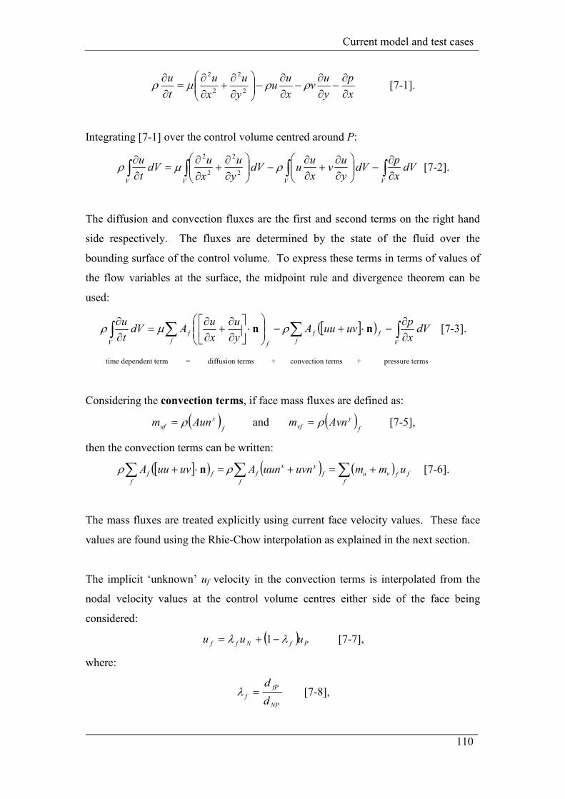
Current model and test cases
110
x
p
y
uv
x
uu
y
u
x
u
t
u
∂∂
−∂∂
−∂∂
−
∂
∂+
∂
∂=
∂∂
ρρµρ2
2
2
2
[7-1].
Integrating [7-1] over the control volume centred around P:
∫∫∫∫ ∂∂
−
∂∂
+∂∂
−
∂
∂+
∂
∂=
∂∂
VVVV
dVx
pdV
y
uv
x
uudV
y
u
x
udV
t
u
2
2
2
2
ρµρ [7-2].
The diffusion and convection fluxes are the first and second terms on the right hand
side respectively. The fluxes are determined by the state of the fluid over the
bounding surface of the control volume. To express these terms in terms of values of
the flow variables at the surface, the midpoint rule and divergence theorem can be
used:
[ ]( ) ∫∑∑∫ ∂∂
−⋅+−
⋅
∂∂
+∂∂
=∂∂
Vf
ff
f f
f
V
dVx
puvuuA
y
u
x
uAdV
t
u nn ρµρ [7-3].
time dependent term = diffusion terms + convection terms + pressure terms
Considering the convection terms, if face mass fluxes are defined as:
( )f
x
uf Aunm ρ= and ( )f
y
vf Avnm ρ= [7-5],
then the convection terms can be written:
[ ]( ) ( ) ( )∑∑∑ +=+=⋅+f
ffvu
f
f
yx
f
f
ff ummuvnuunAuvuuA ρρ n [7-6].
The mass fluxes are treated explicitly using current face velocity values. These face
values are found using the Rhie-Chow interpolation as explained in the next section.
The implicit ‘unknown’ uf velocity in the convection terms is interpolated from the
nodal velocity values at the control volume centres either side of the face being
considered:
( )PfNff uuu λλ −+= 1 [7-7],
where:
NP
fP
fd
d=λ [7-8],
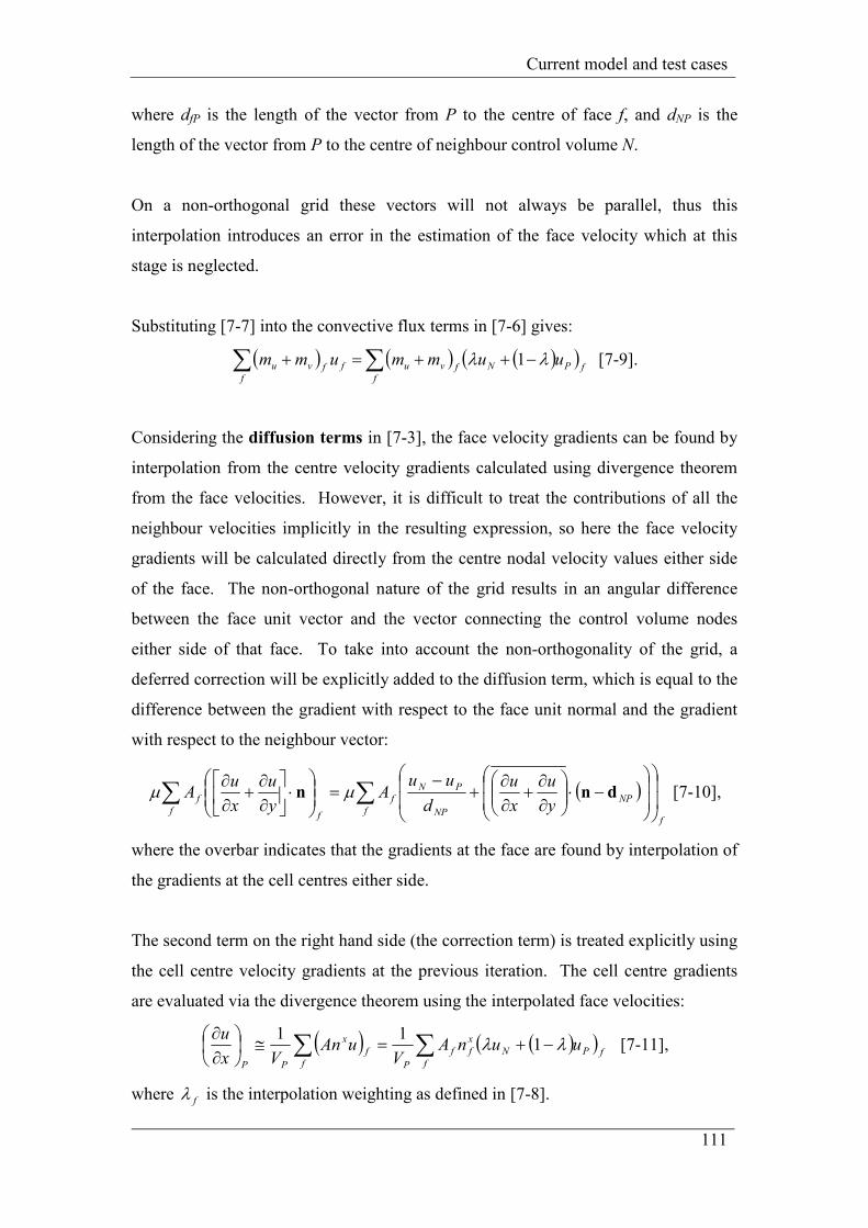
Current model and test cases
111
where dfP is the length of the vector from P to the centre of face f, and dNP is the
length of the vector from P to the centre of neighbour control volume N.
On a non-orthogonal grid these vectors will not always be parallel, thus this
interpolation introduces an error in the estimation of the face velocity which at this
stage is neglected.
Substituting [7-7] into the convective flux terms in [7-6] gives:
( ) ( ) ( )( )∑∑ −++=+f
fPNfvu
f
ffvu uummumm λλ 1 [7-9].
Considering the diffusion terms in [7-3], the face velocity gradients can be found by
interpolation from the centre velocity gradients calculated using divergence theorem
from the face velocities. However, it is difficult to treat the contributions of all the
neighbour velocities implicitly in the resulting expression, so here the face velocity
gradients will be calculated directly from the centre nodal velocity values either side
of the face. The non-orthogonal nature of the grid results in an angular difference
between the face unit vector and the vector connecting the control volume nodes
either side of that face. To take into account the non-orthogonality of the grid, a
deferred correction will be explicitly added to the diffusion term, which is equal to the
difference between the gradient with respect to the face unit normal and the gradient
with respect to the neighbour vector:
( )∑∑
−⋅
∂∂
+∂∂
+−
=
⋅
∂∂
+∂∂
ff
NP
NP
PN
f
f f
fy
u
x
u
d
uuA
y
u
x
uA dnn µµ [7-10],
where the overbar indicates that the gradients at the face are found by interpolation of
the gradients at the cell centres either side.
The second term on the right hand side (the correction term) is treated explicitly using
the cell centre velocity gradients at the previous iteration. The cell centre gradients
are evaluated via the divergence theorem using the interpolated face velocities:
( ) ( )( )∑∑ −+=≅
∂∂
ffPN
x
ff
Pf
f
x
PP
uunAV
uAnVx
uλλ 1
11 [7-11],
where fλ is the interpolation weighting as defined in [7-8].
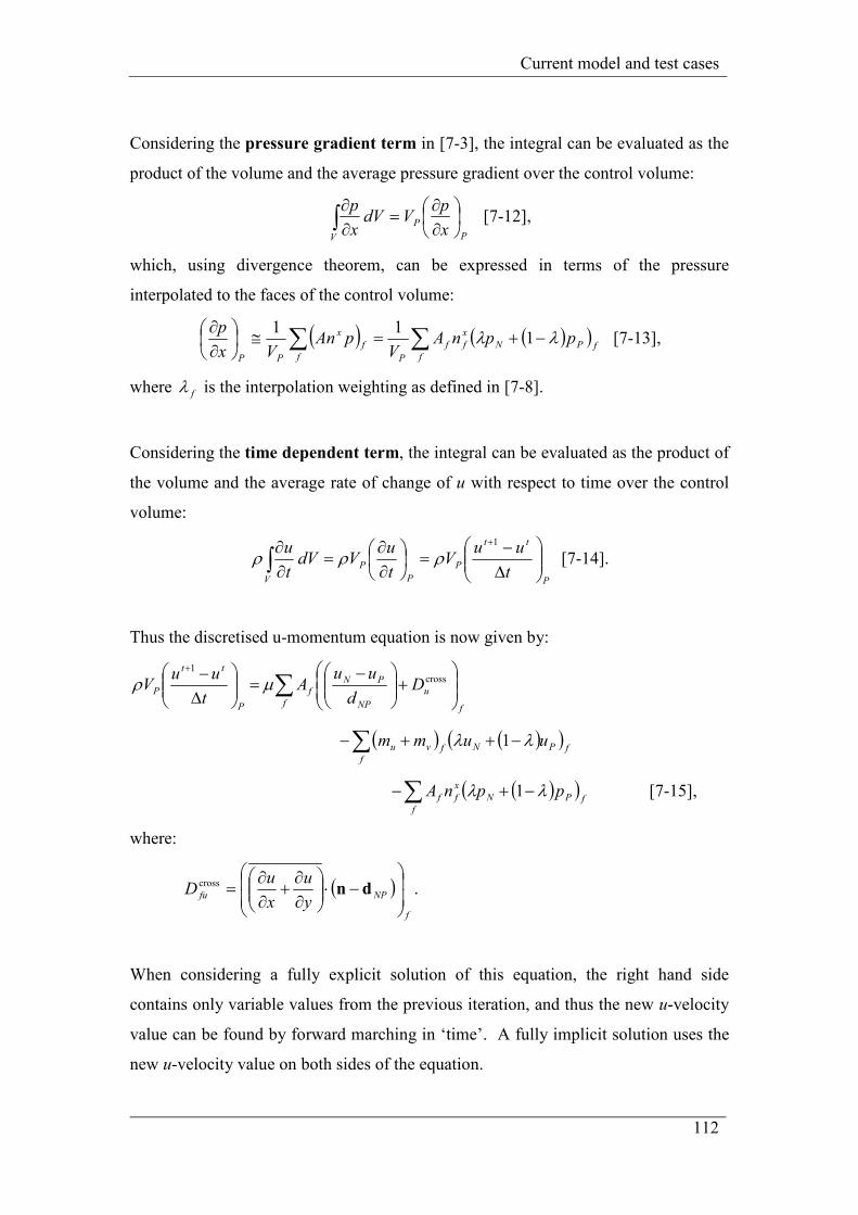
Current model and test cases
112
Considering the pressure gradient term in [7-3], the integral can be evaluated as the
product of the volume and the average pressure gradient over the control volume:
P
P
Vx
pVdV
x
p
∂∂
=∂∂∫ [7-12],
which, using divergence theorem, can be expressed in terms of the pressure
interpolated to the faces of the control volume:
( ) ( )( )∑∑ −+=≅
∂∂
ffPN
x
ff
Pf
f
x
PP
ppnAV
pAnVx
pλλ 1
11 [7-13],
where fλ is the interpolation weighting as defined in [7-8].
Considering the time dependent term, the integral can be evaluated as the product of
the volume and the average rate of change of u with respect to time over the control
volume:
P
tt
P
P
P
Vt
uuV
t
uVdV
t
u
∆−
=
∂∂
=∂∂ +
∫1
ρρρ [7-14].
Thus the discretised u-momentum equation is now given by:
∑
+
−=
∆−+
ff
u
NP
PNf
P
tt
P Dd
uuA
t
uuV cross
1
µρ
( ) ( )( )∑ −++−f
fPNfvu uumm λλ 1
( )( )∑ −+−f
fPN
x
ff ppnA λλ 1 [7-15],
where:
( )f
NPfuy
u
x
uD
−⋅
∂∂
+∂∂
= dncross .
When considering a fully explicit solution of this equation, the right hand side
contains only variable values from the previous iteration, and thus the new u-velocity
value can be found by forward marching in ‘time’. A fully implicit solution uses the
new u-velocity value on both sides of the equation.
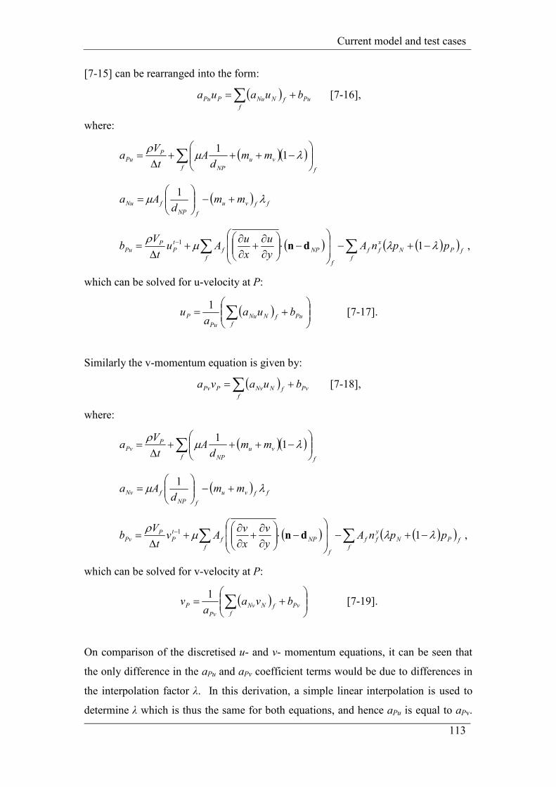
Current model and test cases
113
[7-15] can be rearranged into the form:
( ) Pu
ffNNuPPu buaua +=∑ [7-16],
where:
( )( )∑
−+++
∆=
f f
vu
NP
PPu mm
dA
t
Va λµ
ρ1
1
( ) ffvu
fNP
fNu mmd
Aa λµ +−
=
1
( ) ( )( )∑∑ −+−
−⋅
∂∂
+∂∂
+∆
= −
ffPN
x
ff
ff
NPf
t
PP
Pu ppnAy
u
x
uAu
t
Vb λλµ
ρ11
dn ,
which can be solved for u-velocity at P:
( )
+= ∑
f
PufNNu
Pu
P buaa
u1
[7-17].
Similarly the v-momentum equation is given by:
( ) Pv
ffNNvPPv buava +=∑ [7-18],
where:
( )( )∑
−+++
∆=
f f
vu
NP
PPv mm
dA
t
Va λµ
ρ1
1
( ) ffvu
fNP
fNv mmd
Aa λµ +−
=
1
( ) ( )( )∑∑ −+−
−⋅
∂∂
+∂∂
+∆
= −
ffPN
y
ff
ff
NPf
t
PP
Pv ppnAy
v
x
vAv
t
Vb λλµ
ρ11
dn ,
which can be solved for v-velocity at P:
( )
+= ∑
f
PvfNNv
Pv
P bvaa
v1
[7-19].
On comparison of the discretised u- and v- momentum equations, it can be seen that
the only difference in the aPu and aPv coefficient terms would be due to differences in
the interpolation factor λ. In this derivation, a simple linear interpolation is used to
determine λ which is thus the same for both equations, and hence aPu is equal to aPv.
Current model and test cases
114
If, however, a more complex interpolation scheme were used which used, for
example, up-winding, then a different interpolation factor may result for u and v. By
similar argument aNu is equal to aNv. The source terms, bPu and bPv, are not equal
however, since they contain the term describing the variable u or v at the previous
iteration.
For the solution to a steady state, the u-velocity term, ut-1, in the right-hand source
term, is updated during each iteration, or pseudo-timestep. If the unsteady solution is
being studied, ut-1 is held constant during each iteration and is set equal to the u-
velocity at the previous time-step.
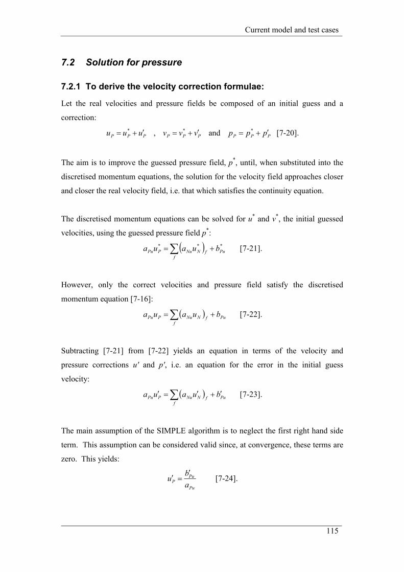
Current model and test cases
115
7.2 Solution for pressure
7.2.1 To derive the velocity correction formulae:
Let the real velocities and pressure fields be composed of an initial guess and a
correction:
PPP uuu ′+= * , PPP vvv ′+= * and PPP ppp ′+= * [7-20].
The aim is to improve the guessed pressure field, p*, until, when substituted into the
discretised momentum equations, the solution for the velocity field approaches closer
and closer the real velocity field, i.e. that which satisfies the continuity equation.
The discretised momentum equations can be solved for u* and v
*, the initial guessed
velocities, using the guessed pressure field p*:
( )∑ +=f
PufNNuPPu buaua *** [7-21].
However, only the correct velocities and pressure field satisfy the discretised
momentum equation [7-16]:
( ) Pu
ffNNuPPu buaua +=∑ [7-22].
Subtracting [7-21] from [7-22] yields an equation in terms of the velocity and
pressure corrections u' and p', i.e. an equation for the error in the initial guess
velocity:
( ) Pu
ffNNuPPu buaua ′+′=′ ∑ [7-23].
The main assumption of the SIMPLE algorithm is to neglect the first right hand side
term. This assumption can be considered valid since, at convergence, these terms are
zero. This yields:
Pu
PuP
a
bu
′=′ [7-24].
Current model and test cases
116
Considering the discretised momentum equation described earlier, the source terms,
bPu in [7-21] – [7-24] are, in the general case, of the form:
source = time dependent
term contribution +
cross-diffusion
term contribution +
pressure gradient
term contribution
Since the time dependent term and the cross-diffusion term use velocity values from
the previous iteration (i.e. are treated explicitly), there is no correction needed to these
velocities, so the only term in the b'Pu term is a function of the pressure correction
needed:
P
PPux
pVb
∂
′∂−=′ [7-25],
in which, by the divergence theorem as in [7-13], the pressure correction gradient can
be expressed in terms of the interpolated control volume face pressure values:
( ) ( )( )∑∑ ′−+′=′≅
∂
′∂
ffPN
x
ff
Pf
f
x
PP
ppnAV
pAnVx
pλλ 1
11 [7-26].
Thus substitution of [7-25] and [7-26] into [7-24] gives an expression describing the
velocity corrections, u'P, in terms of the pressure corrections, p'P:
( )( )
′−+′−=′ ∑
ffPN
x
ff
Pu
P ppnAa
u λλ 11
[7-27].
7.2.2 To derive the equation for pressure correction:
Considering the equation of conservation of mass (the continuity equation) [2-9]:
0=∂∂
+∂∂
y
v
x
u [7-28].
Integrating over the control volume yields:
0 =∂∂
+∂∂
∫∫VV
dVy
vdV
x
u [7-29],
which, following the same procedure as [7-2] – [7-3] using divergence theorem and
midpoint rule to convert the integral to a discrete sum, gives:
[ ]( )( )∑ =⋅+f
fvuA 0n [7-30],
Current model and test cases
117
which is equivalent to:
( )( ) 0=+∑f
f
yx vnunA [7-31].
Let the velocities be composed of an initial guess and the correction as defined by
[7-20], [7-25] and [7-26]:
PPu
PPP
x
p
a
Vuu
∂
′∂−= * and
PPv
PPP
y
p
a
Vvv
∂
′∂−= * [7-32],
which can be interpolated to the faces of the control volume:
ffu
f
ffx
p
a
Vuu
∂
′∂−= * and
ffv
f
ffy
p
a
Vvv
∂
′∂−= * [7-33],
where:
( )Pu
Pf
Nu
Nf
fu
f
a
V
a
V
a
Vλλ −+= 1 and ( )
Pv
Pf
Nv
Nf
fv
f
a
V
a
V
a
Vλλ −+= 1 [7-34],
in which the aP term is the central coefficient of the momentum equation for control
volume P and aN is the central coefficient of the momentum equation for control
volume N (i.e. not the neighbour coefficient).
Substituting into [7-31] yields:
0** =
∂
′∂−+
∂
′∂−∑
f
y
f
ffv
f
f
x
f
ffu
f
ff ny
p
a
Vvn
x
p
a
VuA [7-35].
The pressure correction gradients can be evaluated at the control volume face as
follows:
( )( )( ) ( )22
PNPN
PNPN
f yyxx
xxpp
x
p
−+−
−′−′=
∂
′∂ and
( )( )( ) ( )22
PNPN
PNPN
fyyxx
yypp
y
p
−+−
−′−′=
∂
′∂ [7-36],
which gives:
( )( )( ) ( )
( )( )( ) ( )∑ =
−+−
−′−′−+
−+−
−′−′−
f
y
f
fPNPN
PNPN
fv
f
f
x
f
fPNPN
PNPN
fu
f
ff nyyxx
yypp
a
Vvn
yyxx
xxpp
a
VuA 0
22
*
22
*
[7-37].
Considering the afu term in [7-37]:
Current model and test cases
118
( ) ( )( )PPufNPuffu aaa λλ −+= 1 [7-38],
in which, from [7-16]:
( )( )∑
−+++
∆=
f f
vu
NP
PPu mm
dA
t
Va λµ
ρ1
1 [7-39].
From [7-16] and [7-18] it can be seen that PvPu aa = , and, since the same interpolation
factor, λf is used for the u- and v- interpolation, ffvfu aaa == [7-40].
[7-37] can be rearranged into the form:
( ) Pp
ffNNpPPp bpapa +′=′ ∑ [7-41],
where:
( ) ( )( ) ( )∑
−+−
−+−=
f PNPN
y
fPN
x
fPN
f
f
fPpyyxx
nyynxx
a
VAa
22
( ) ( )( ) ( )
−+−
−+−=
22
PNPN
y
fPN
x
fPN
f
f
fNpyyxx
nyynxx
a
VAa
( )( ) ( )∑ ∑ +−=+−=f f
vuf
yx
Pp mmnvnuAb **** ,
where af is as defined in [7-38] – [7-40], Vf is interpolate as in [7-34].
This equation is solved iteratively for p' at control volume centres.
The mass flux terms in the bPp source term must be carefully evaluated to avoid the
problems associated with pressure and velocity coupling on a collocated grid. The
Rhie-Chow interpolation evaluates the mass fluxes as follows.
Given that:
( ) fx
fu Aunm ρ= and ( ) fy
fv Avnm ρ= [7-42],
after Rhie & Chow (1983), the face velocities are treated explicitly as:
∂∂
−
∂∂
−=
fffP
Pff
x
p
x
p
a
Vuu * and
∂∂
−
∂∂
−=
fffP
Pff
y
p
y
p
a
Vvv * [7-
43],
Current model and test cases
119
where the overbar terms are found by linear interpolation of the values at the centre
nodes either side of face f:
( ) *** 1 PfNff uuu λλ −+= [7-44]
( )PP
Pf
NP
Pf
fP
P
a
V
a
V
a
V
−+
=
λλ 1 [7-45]
( )P
f
N
f
f x
p
x
p
x
p
∂∂
−+
∂∂
=
∂∂
λλ 1 and ( )P
f
N
f
fy
p
y
p
y
p
∂∂
−+
∂∂
=
∂∂
λλ 1 [7-
46].
The first pressure gradient term in [7-43] is found from the pressure values at the
centre nodes:
( )( )( ) ( )
( ) x
f
NP
PN
PNPN
PNPN
f
nd
pp
yyxx
xxpp
x
p −=
−+−
−−=
∂∂
22
and ( )( )
( ) ( )( ) y
f
NP
PN
PNPN
PNPN
f
nd
pp
yyxx
yypp
y
p −=
−+−
−−=
∂∂
22 [7-47].
Using [7-43] the face total mass flux terms in bPp in [7-34] can be defined:
( )
( )
∂∂
+∂∂
−
∂∂
+∂∂
−+=
∂∂
−
∂∂
−+
∂∂
−
∂∂
−=+=
fffP
Pfff
fffP
Pf
fffP
Pff
y
f
x
ff
y
p
x
p
y
p
x
p
a
VvuA
y
p
y
p
a
Vv
x
p
x
p
a
VuAmm
**
**
ρ
ρm
[7-48].
To update the velocities use [7-32] in which the p' gradient terms are evaluated by
considering the average over the control volume, as in [7-12] – [7-13], which, using
divergence theorem, can be expressed in terms of the pressure interpolated to the
faces of the control volume:
( ) ( )( )∑∑ ′−+′=′≅
∂
′∂
ffPN
x
ff
Pf
f
x
PP
ppnAV
pAnVx
pλλ 1
11 [7-49],
where λ is as defined in [7-8].
Current model and test cases
120
Substituting into [7-32]:
( )( )∑ ′−+′+=f
fPN
x
ff
P
PP ppnAa
uu λλ 11*
and ( )( )∑ ′−+′+=f
fPN
y
ff
P
PP ppnAa
vv λλ 11* [7-50].
The pressures can be updated similarly:
PPP ppp ′+= * [7-51].
It is necessary to under-relax both the velocity and pressure updates due to the
simplifying assumptions made in the SIMPLE formulation.
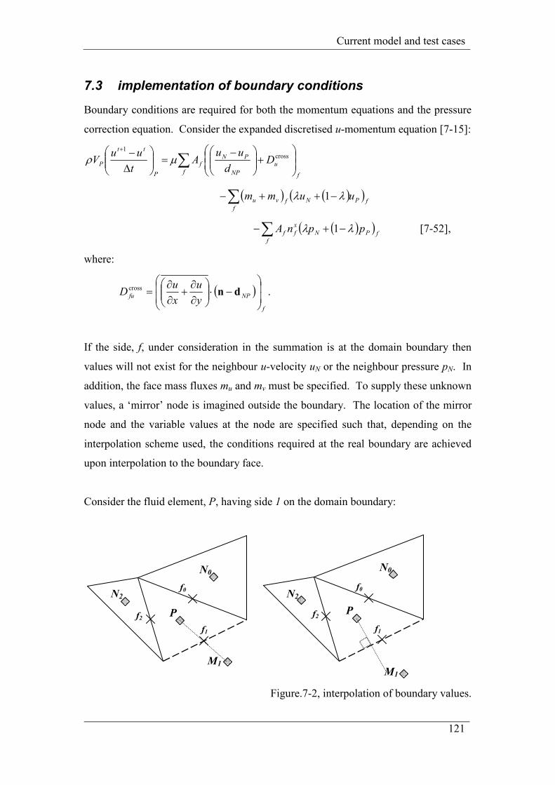
Current model and test cases
121
7.3 implementation of boundary conditions
Boundary conditions are required for both the momentum equations and the pressure
correction equation. Consider the expanded discretised u-momentum equation [7-15]:
∑
+
−=
∆−+
ff
u
NP
PNf
P
tt
P Dd
uuA
t
uuV cross
1
µρ
( ) ( )( )∑ −++−f
fPNfvu uumm λλ 1
( )( )∑ −+−f
fPN
x
ff ppnA λλ 1 [7-52],
where:
( )f
NPfuy
u
x
uD
−⋅
∂∂
+∂∂
= dncross .
If the side, f, under consideration in the summation is at the domain boundary then
values will not exist for the neighbour u-velocity uN or the neighbour pressure pN. In
addition, the face mass fluxes mu and mv must be specified. To supply these unknown
values, a ‘mirror’ node is imagined outside the boundary. The location of the mirror
node and the variable values at the node are specified such that, depending on the
interpolation scheme used, the conditions required at the real boundary are achieved
upon interpolation to the boundary face.
Consider the fluid element, P, having side 1 on the domain boundary:
Figure.7-2, interpolation of boundary values.
M1
N2
N0
P
f0
f2
f1
N0
M1
P
N2
f2
f0
f1
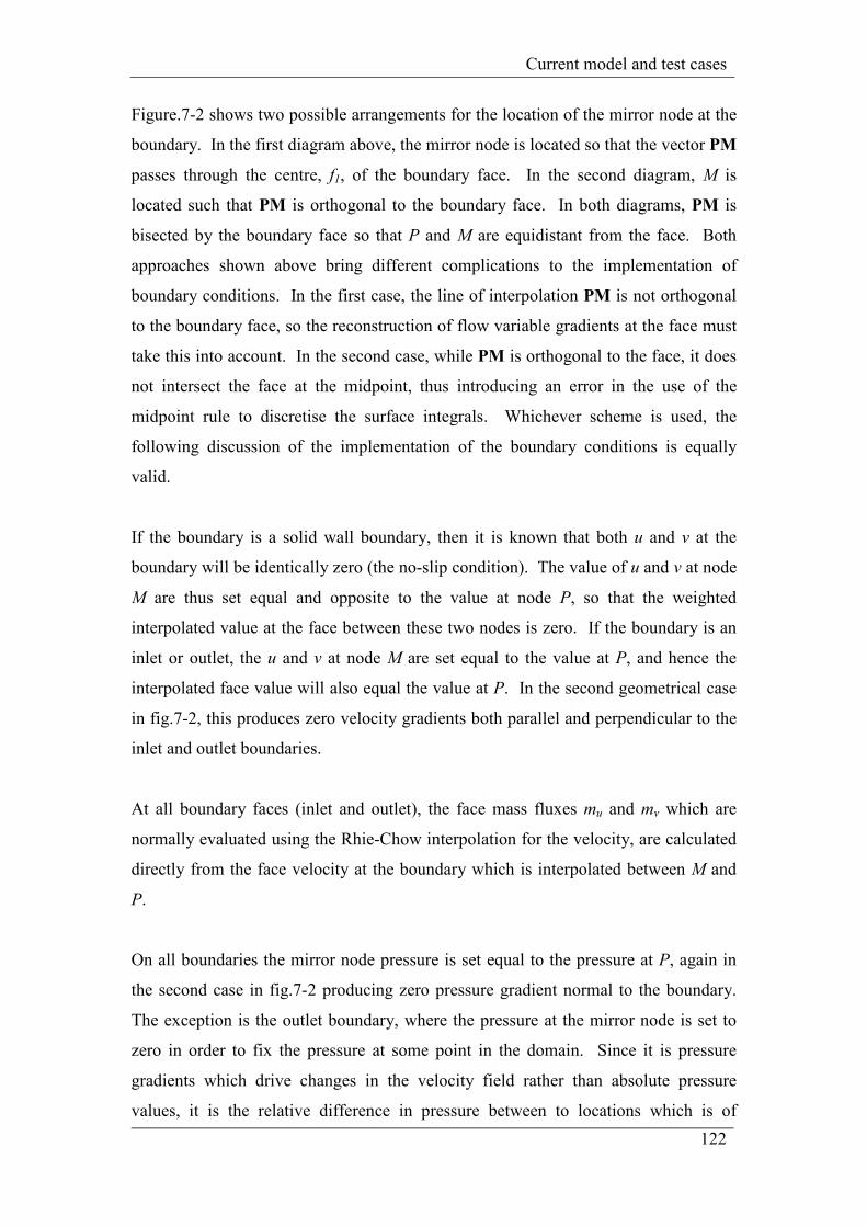
Current model and test cases
122
Figure.7-2 shows two possible arrangements for the location of the mirror node at the
boundary. In the first diagram above, the mirror node is located so that the vector PM
passes through the centre, f1, of the boundary face. In the second diagram, M is
located such that PM is orthogonal to the boundary face. In both diagrams, PM is
bisected by the boundary face so that P and M are equidistant from the face. Both
approaches shown above bring different complications to the implementation of
boundary conditions. In the first case, the line of interpolation PM is not orthogonal
to the boundary face, so the reconstruction of flow variable gradients at the face must
take this into account. In the second case, while PM is orthogonal to the face, it does
not intersect the face at the midpoint, thus introducing an error in the use of the
midpoint rule to discretise the surface integrals. Whichever scheme is used, the
following discussion of the implementation of the boundary conditions is equally
valid.
If the boundary is a solid wall boundary, then it is known that both u and v at the
boundary will be identically zero (the no-slip condition). The value of u and v at node
M are thus set equal and opposite to the value at node P, so that the weighted
interpolated value at the face between these two nodes is zero. If the boundary is an
inlet or outlet, the u and v at node M are set equal to the value at P, and hence the
interpolated face value will also equal the value at P. In the second geometrical case
in fig.7-2, this produces zero velocity gradients both parallel and perpendicular to the
inlet and outlet boundaries.
At all boundary faces (inlet and outlet), the face mass fluxes mu and mv which are
normally evaluated using the Rhie-Chow interpolation for the velocity, are calculated
directly from the face velocity at the boundary which is interpolated between M and
P.
On all boundaries the mirror node pressure is set equal to the pressure at P, again in
the second case in fig.7-2 producing zero pressure gradient normal to the boundary.
The exception is the outlet boundary, where the pressure at the mirror node is set to
zero in order to fix the pressure at some point in the domain. Since it is pressure
gradients which drive changes in the velocity field rather than absolute pressure
values, it is the relative difference in pressure between to locations which is of
Current model and test cases
123
interest, thus the pressure field in the converged solution shall be described relative to
this fixed point.
The mirror node values are included in the bPu source term in the discretised
momentum equations. Since the mirror flow values are functions of the flow values
at the computational node P being considered, they are treated explicitly using values
from the previous iteration.
Boundary conditions are also required for the solution of the pressure correction
equation [7-37]:
( )( )( ) ( )
( )( )( ) ( )∑ =
−+−
−′−′−+
−+−
−′−′−
f
y
f
fPNPN
PNPN
fv
f
f
x
f
fPNPN
PNPN
fu
f
ff nyyxx
yypp
a
Vvn
yyxx
xxpp
a
VuA 0
22
*
22
*
[7-53].
The same boundary conditions are applied to the pressure corrections as to the
pressure in the momentum equations; the mirror node pressure correction is set equal
to the internal node pressure correction, except on the outlet boundary where it is set
to zero. Furthermore, the boundary face velocity is known and therefore requires no
correction. Again, the mirror node contributions are included in the source term and
are treated explicitly using flow values from the previous iteration.
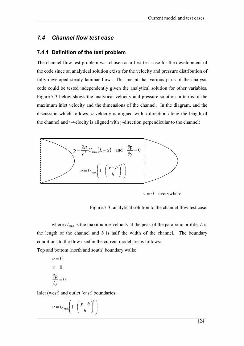
Current model and test cases
124
7.4 Channel flow test case
7.4.1 Definition of the test problem
The channel flow test problem was chosen as a first test case for the development of
the code since an analytical solution exists for the velocity and pressure distribution of
fully developed steady laminar flow. This meant that various parts of the analysis
code could be tested independently given the analytical solution for other variables.
Figure.7-3 below shows the analytical velocity and pressure solution in terms of the
maximum inlet velocity and the dimensions of the channel. In the diagram, and the
discussion which follows, u-velocity is aligned with x-direction along the length of
the channel and v-velocity is aligned with y-direction perpendicular to the channel:
Figure.7-3, analytical solution to the channel flow test case.
where Umax is the maximum u-velocity at the peak of the parabolic profile, L is
the length of the channel and b is half the width of the channel. The boundary
conditions to the flow used in the current model are as follows:
Top and bottom (north and south) boundary walls:
0=u
0=v
0=∂
∂
y
p
Inlet (west) and outlet (east) boundaries:
−−=
2
max 1b
byUu
−−=
2
max 1b
byUu
everywhere 0=v
( ) 0y
p and
2p max2
=∂∂
−= xLUb
µ
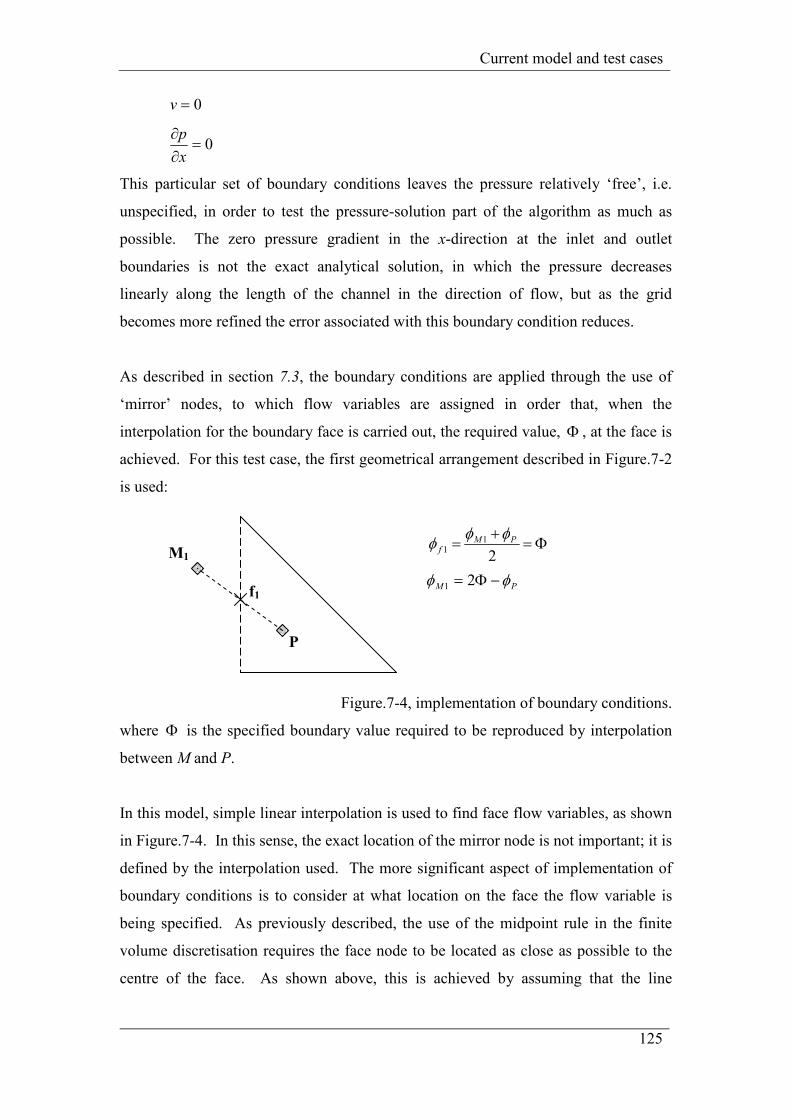
Current model and test cases
125
0=v
0=∂
∂
x
p
This particular set of boundary conditions leaves the pressure relatively ‘free’, i.e.
unspecified, in order to test the pressure-solution part of the algorithm as much as
possible. The zero pressure gradient in the x-direction at the inlet and outlet
boundaries is not the exact analytical solution, in which the pressure decreases
linearly along the length of the channel in the direction of flow, but as the grid
becomes more refined the error associated with this boundary condition reduces.
As described in section 7.3, the boundary conditions are applied through the use of
‘mirror’ nodes, to which flow variables are assigned in order that, when the
interpolation for the boundary face is carried out, the required value, Φ , at the face is
achieved. For this test case, the first geometrical arrangement described in Figure.7-2
is used:
Figure.7-4, implementation of boundary conditions.
where Φ is the specified boundary value required to be reproduced by interpolation
between M and P.
In this model, simple linear interpolation is used to find face flow variables, as shown
in Figure.7-4. In this sense, the exact location of the mirror node is not important; it is
defined by the interpolation used. The more significant aspect of implementation of
boundary conditions is to consider at what location on the face the flow variable is
being specified. As previously described, the use of the midpoint rule in the finite
volume discretisation requires the face node to be located as close as possible to the
centre of the face. As shown above, this is achieved by assuming that the line
M1
f1
P
Φ=+
=2
11
PMf
φφφ
PM φφ −Φ= 21
Current model and test cases
126
connecting the control volume computational node P to the mirror node M passes
through the centre of the boundary face.
However, this is balanced against the requirement that the line connecting P and M
along which the interpolation is carried out be perpendicular to the boundary face.
This introduces an error in cases where the derivative of a variable is specified in the
boundary condition, since the direction along which the values of the variable are
known is not necessarily the direction in which the condition is specified. This is
similar to the issues involved with calculating diffusive fluxes on non-orthogonal
grids. The implications of this will be discussed further in the next chapter.
For this test case, it was found that the location of the face node has a much greater
influence over the accuracy of the solution (due to the loss of accuracy of the
midpoint rule should this node not be at the centre of the face) compared to the impact
of extrapolating along non-orthogonal lines. Therefore the scheme shown in the
diagram above was used.
The parameters of the flow test case are:
channel width 1.0
channel length 2.0
viscosity 0.1
density 1.0
Umax 1.0
grid size 60 cells in x-direction (along the channel) by 30 cells in y-direction (across
the channel) which form 1800 square cells, each then divided into two triangles giving
3600 CVs overall.
Which gives a Reynolds number for the flow (based on the channel width) of 10, and
a cell Peclet number of 0.33.
A steady state solution is used and the velocities are updated each iteration. A
pseudo-timestep iteration is used, defined as:
max
1.0U
xt
∆=∆ [7-54]
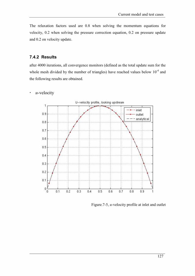
Current model and test cases
127
The relaxation factors used are 0.8 when solving the momentum equations for
velocity, 0.2 when solving the pressure correction equation, 0.2 on pressure update
and 0.2 on velocity update.
7.4.2 Results
after 4000 iterations, all convergence monitors (defined as the total update sum for the
whole mesh divided by the number of triangles) have reached values below 10-4 and
the following results are obtained.
u-velocity
Figure.7-5, u-velocity profile at inlet and outlet
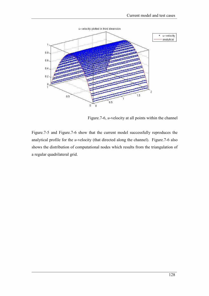
Current model and test cases
128
Figure.7-6, u-velocity at all points within the channel
Figure.7-5 and Figure.7-6 show that the current model successfully reproduces the
analytical profile for the u-velocity (that directed along the channel). Figure.7-6 also
shows the distribution of computational nodes which results from the triangulation of
a regular quadrilateral grid.
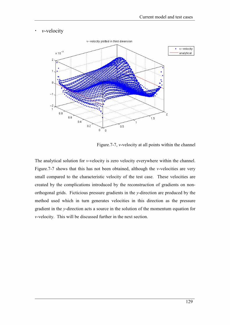
Current model and test cases
129
v-velocity
Figure.7-7, v-velocity at all points within the channel
The analytical solution for v-velocity is zero velocity everywhere within the channel.
Figure.7-7 shows that this has not been obtained, although the v-velocities are very
small compared to the characteristic velocity of the test case. These velocities are
created by the complications introduced by the reconstruction of gradients on non-
orthogonal grids. Ficticious pressure gradients in the y-direction are produced by the
method used which in turn generates velocities in this direction as the pressure
gradient in the y-direction acts a source in the solution of the momentum equation for
v-velocity. This will be discussed further in the next section.
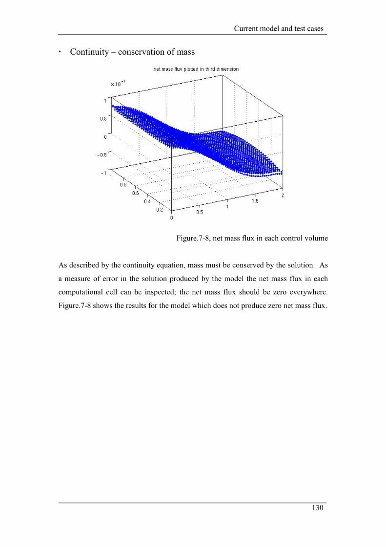
Current model and test cases
130
Continuity – conservation of mass
Figure.7-8, net mass flux in each control volume
As described by the continuity equation, mass must be conserved by the solution. As
a measure of error in the solution produced by the model the net mass flux in each
computational cell can be inspected; the net mass flux should be zero everywhere.
Figure.7-8 shows the results for the model which does not produce zero net mass flux.
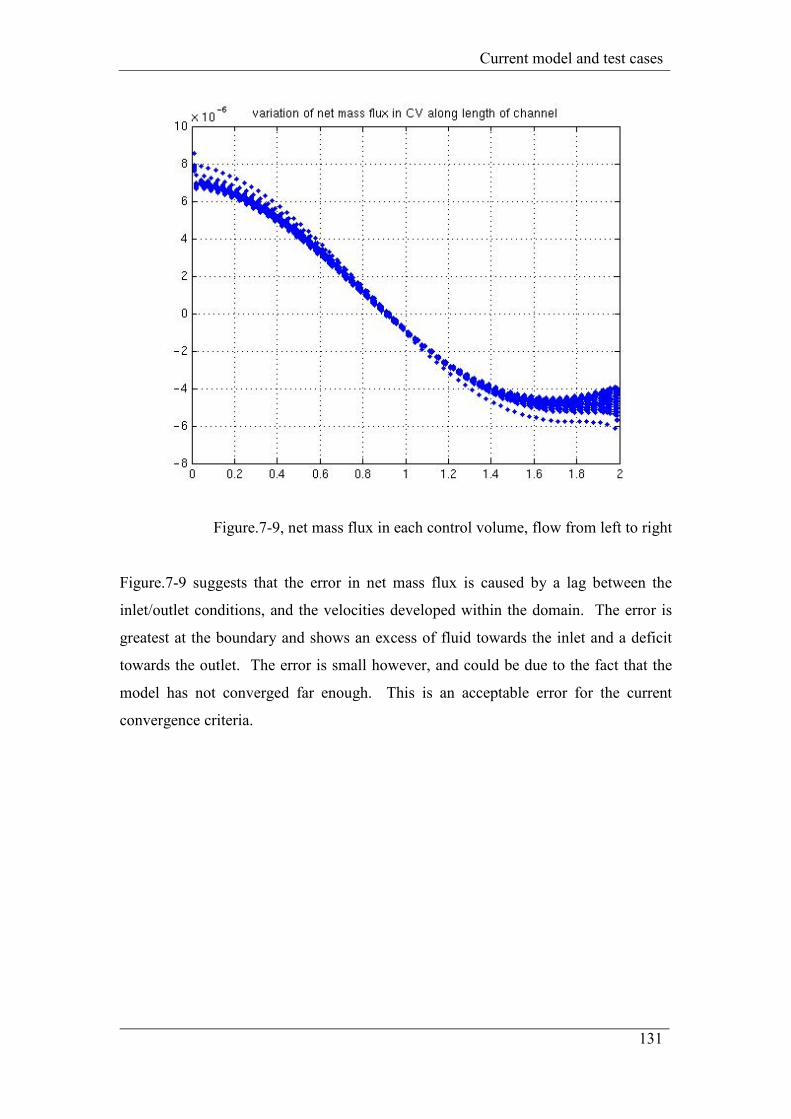
Current model and test cases
131
Figure.7-9, net mass flux in each control volume, flow from left to right
Figure.7-9 suggests that the error in net mass flux is caused by a lag between the
inlet/outlet conditions, and the velocities developed within the domain. The error is
greatest at the boundary and shows an excess of fluid towards the inlet and a deficit
towards the outlet. The error is small however, and could be due to the fact that the
model has not converged far enough. This is an acceptable error for the current
convergence criteria.
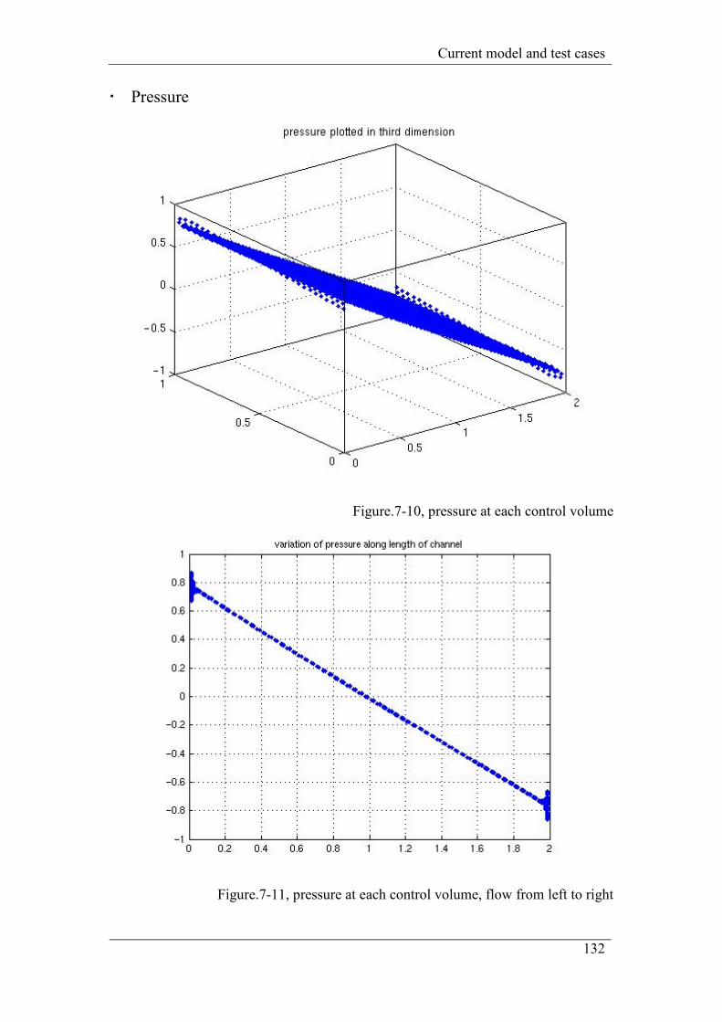
Current model and test cases
132
Pressure
Figure.7-10, pressure at each control volume
Figure.7-11, pressure at each control volume, flow from left to right
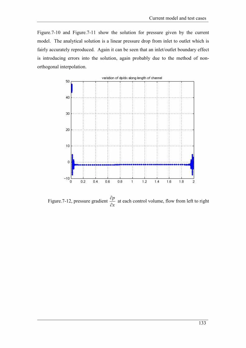
Current model and test cases
133
Figure.7-10 and Figure.7-11 show the solution for pressure given by the current
model. The analytical solution is a linear pressure drop from inlet to outlet which is
fairly accurately reproduced. Again it can be seen that an inlet/outlet boundary effect
is introducing errors into the solution, again probably due to the method of non-
orthogonal interpolation.
Figure.7-12, pressure gradient x
p
∂
∂ at each control volume, flow from left to right
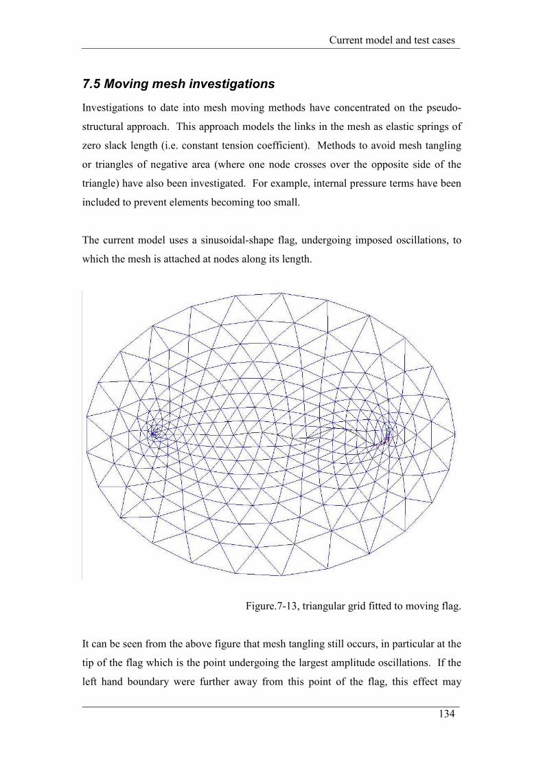
Current model and test cases
134
7.5 Moving mesh investigations
Investigations to date into mesh moving methods have concentrated on the pseudo-
structural approach. This approach models the links in the mesh as elastic springs of
zero slack length (i.e. constant tension coefficient). Methods to avoid mesh tangling
or triangles of negative area (where one node crosses over the opposite side of the
triangle) have also been investigated. For example, internal pressure terms have been
included to prevent elements becoming too small.
The current model uses a sinusoidal-shape flag, undergoing imposed oscillations, to
which the mesh is attached at nodes along its length.
Figure.7-13, triangular grid fitted to moving flag.
It can be seen from the above figure that mesh tangling still occurs, in particular at the
tip of the flag which is the point undergoing the largest amplitude oscillations. If the
left hand boundary were further away from this point of the flag, this effect may
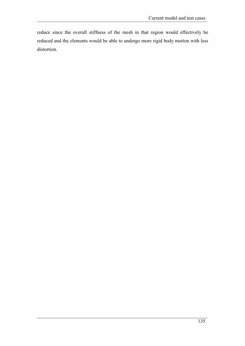
Current model and test cases
135
reduce since the overall stiffness of the mesh in that region would effectively be
reduced and the elements would be able to undergo more rigid body motion with less
distortion.
Proposed developments to the current model
136
8 Proposed development of the current model
The current model calculates the steady flow of an incompressible viscous fluid as
presented in the previous chapter. In order to model the interactions of the fluid with
a flexible structure a number of developments are required which will now be
described.
The model must be able to predict the separation of the flow from the surface of the
structure and the zones of recirculation that form as described in sections 2.1.4 and
2.5.1. The algorithm must be extended to carry out unsteady flow analysis. The
current model uses the time dependent terms in the momentum equation to aid
stability on the progression to a steady solution. In an unsteady analysis these terms
will be updated correctly based on the flow solution at the previous time step. The
timestep size and time integration technique are closely related each other and their
influence on the stability and accuracy of the solution has been described in sections
5.2 and 5.4. Moving domain boundaries present further challenges as the boundary-
conforming computational mesh must be moved and updated under the influence of
the boundary motion. Techniques for controlling mesh movements were presented in
chapter 6. Lastly, the fluid and structure systems must be coupled to produce the
displacements and deformations of the fluid-structure interface as part of the coupled
solution.
A number of different test cases will be used to develop the model in the stages
required as described above.
8.1 Test case with separation
A test case must be developed to validate the capability of the computational fluid
dynamics code to predict boundary layer separation. The test case of flow over a flat
plate normal to the flow direction will be used for this purpose.
Up to a critical (very low) Reynolds number, of the order Re=20, the flow will remain
steady with a symmetrical pair of standing vortices attached to the plate. If the flow
velocity is increased (i.e. Re is increased), the vortex pair will begin to oscillate until,
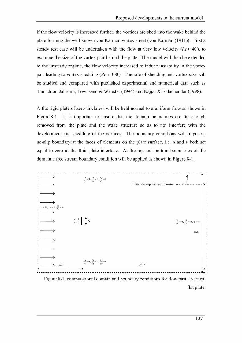
Proposed developments to the current model
137
if the flow velocity is increased further, the vortices are shed into the wake behind the
plate forming the well known von Kármán vortex street (von Kármán (1911)). First a
steady test case will be undertaken with the flow at very low velocity (Re 40≈ ), to
examine the size of the vortex pair behind the plate. The model will then be extended
to the unsteady regime, the flow velocity increased to induce instability in the vortex
pair leading to vortex shedding (Re 300≈ ). The rate of shedding and vortex size will
be studied and compared with published experimental and numerical data such as
Tamaddon-Jahromi, Townsend & Webster (1994) and Najjar & Balachandar (1998).
A flat rigid plate of zero thickness will be held normal to a uniform flow as shown in
Figure.8-1. It is important to ensure that the domain boundaries are far enough
removed from the plate and the wake structure so as to not interfere with the
development and shedding of the vortices. The boundary conditions will impose a
no-slip boundary at the faces of elements on the plate surface, i.e. u and v both set
equal to zero at the fluid-plate interface. At the top and bottom boundaries of the
domain a free stream boundary condition will be applied as shown in Figure.8-1.
Figure.8-1, computational domain and boundary conditions for flow past a vertical
flat plate.
H
limits of computational domain
5H 20H
16H
0
0
=
=
v
u
0 , 0 , 0 =∂∂
=∂∂
=∂∂
y
p
y
v
y
u
0 , 0 , 0 =∂∂
=∂∂
=∂∂
y
p
y
v
y
u
0 , 0 , =∂
∂== ∞
x
pvUu
00 , 0 ==∂
∂=
∂
∂ , p
x
v
x
u
Proposed developments to the current model
138
The steady problem will test the ability of the code to predict the separation and
recirculation of the flow, and leads conveniently into the extension of the code for
unsteady analysis. The unsteady case presents the further challenge of choice of
timestep size and time integration method (i.e. degree of implicit treatment of
unknowns) which must be investigated to ensure the maximum accuracy and stability
of the solution. A further important factor in the development of the model is that this
test case includes a zero thickness wall boundary which will represent the flexible
membrane in the final model. It will be important to develop techniques to include
this type of internal boundary while ensuring that information from the appropriate
control volumes is used when considering the flow near the interface, i.e. that no
cross-over of information occurs from one side of the plate to the other.
8.2 Test case with mesh motion
The project will investigate mesh motion control algorithms, based on the pseudo-
structure spring analogy, including techniques for avoiding mesh tangling and
extremely high aspect ratio cells. Techniques such as nodal torsional springs, or
internal inflation pressures will be investigated, along with methods for increasing or
decreasing mesh density where needed in the solution domain through manipulation
of the pseudo-structural qualities of the mesh.
The fluid equations of motion will be reformulated to take into account the mesh
motion while ensuring preservation of the geometric conservation law. The geometric
conservation law, first formulated by Thomas & Lombard (1979) sates that, in a
computational fluid dynamics model using moving meshes, the interpretation and use
of the data regarding the mesh location and velocities must be such that the change in
volume of a fluid control volume from one time step to the next is equal to the total
volume swept by the faces of the control volume during that timestep.
∫∫ ⋅=SV
ddVdt
dSw [8-1],
where w is the velocity of the control volume boundary face.
This means that there must be an agreement between the cell volumes used in
calculations, and the method of calculation of face fluxes. The implications of the
Proposed developments to the current model
139
geometric conservation law vary between different applications since it is dependent
on the numerical procedures applied in each case.
A good test case would be to recreate the uniform steady flow in a two dimensional
channel using a mesh which is undergoing arbitrary motions. The solution can then
be compared with the analysis already carried out using a stationary mesh. A similar
analysis has been carried out by Kamakoti & Shyy (2004a). This case would
demonstrate the error in the solution associated with the treatment of the geometric
conservation law.
A further moving mesh test case proposed is the analysis of flow around a moving
zero thickness plate as shown in Figure.8-2 below. The plate is forced to oscillate
about the leading edge point which remains pinned and stationary. In this test case
the adaptation of the mesh density according to the flow solution will be investigated.
As previously explained in chapter 6, accuracy of the solution can be improved by
decreasing the spacing between computational nodes in areas of the solution where
the detail of the flow structure is particularly fine or where the flow variables are
varying rapidly. Various methods of controlling this mesh adaptation will be
investigated including forcing mesh concentration in areas of high vorticity.
A further challenge associated with this test case is the implementation of boundary
conditions at boundaries aligned arbitrarily with respect to the velocity components
used. In all previous models the wall boundaries have been aligned with either u or v
which simplifies the boundary conditions at the face since simple extrapolations can
be used. The method of reconstructing the velocity gradients at an arbitrarily oriented
boundary must be investigated. The boundary conditions will have to be reformulated
in local coordinates, perpendicular and parallel to the wall orientation at that point.
The implementation of boundary conditions is closely related to the interfacing
method as will be discussed below.
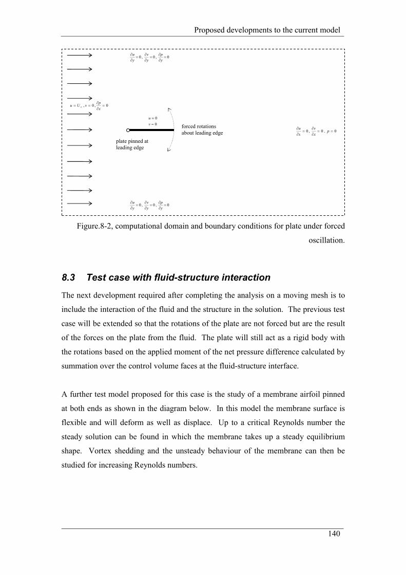
Proposed developments to the current model
140
Figure.8-2, computational domain and boundary conditions for plate under forced
oscillation.
8.3 Test case with fluid-structure interaction
The next development required after completing the analysis on a moving mesh is to
include the interaction of the fluid and the structure in the solution. The previous test
case will be extended so that the rotations of the plate are not forced but are the result
of the forces on the plate from the fluid. The plate will still act as a rigid body with
the rotations based on the applied moment of the net pressure difference calculated by
summation over the control volume faces at the fluid-structure interface.
A further test model proposed for this case is the study of a membrane airfoil pinned
at both ends as shown in the diagram below. In this model the membrane surface is
flexible and will deform as well as displace. Up to a critical Reynolds number the
steady solution can be found in which the membrane takes up a steady equilibrium
shape. Vortex shedding and the unsteady behaviour of the membrane can then be
studied for increasing Reynolds numbers.
plate pinned at
leading edge
forced rotations
about leading edge
0
0
=
=
v
u
0 , 0 , 0 =∂∂
=∂∂
=∂∂
y
p
y
v
y
u
0 , 0 , 0 =∂∂
=∂∂
=∂∂
y
p
y
v
y
u
0 , 0 , =∂
∂== ∞
x
pvUu
00 , 0 ==∂
∂=
∂
∂ , p
x
v
x
u
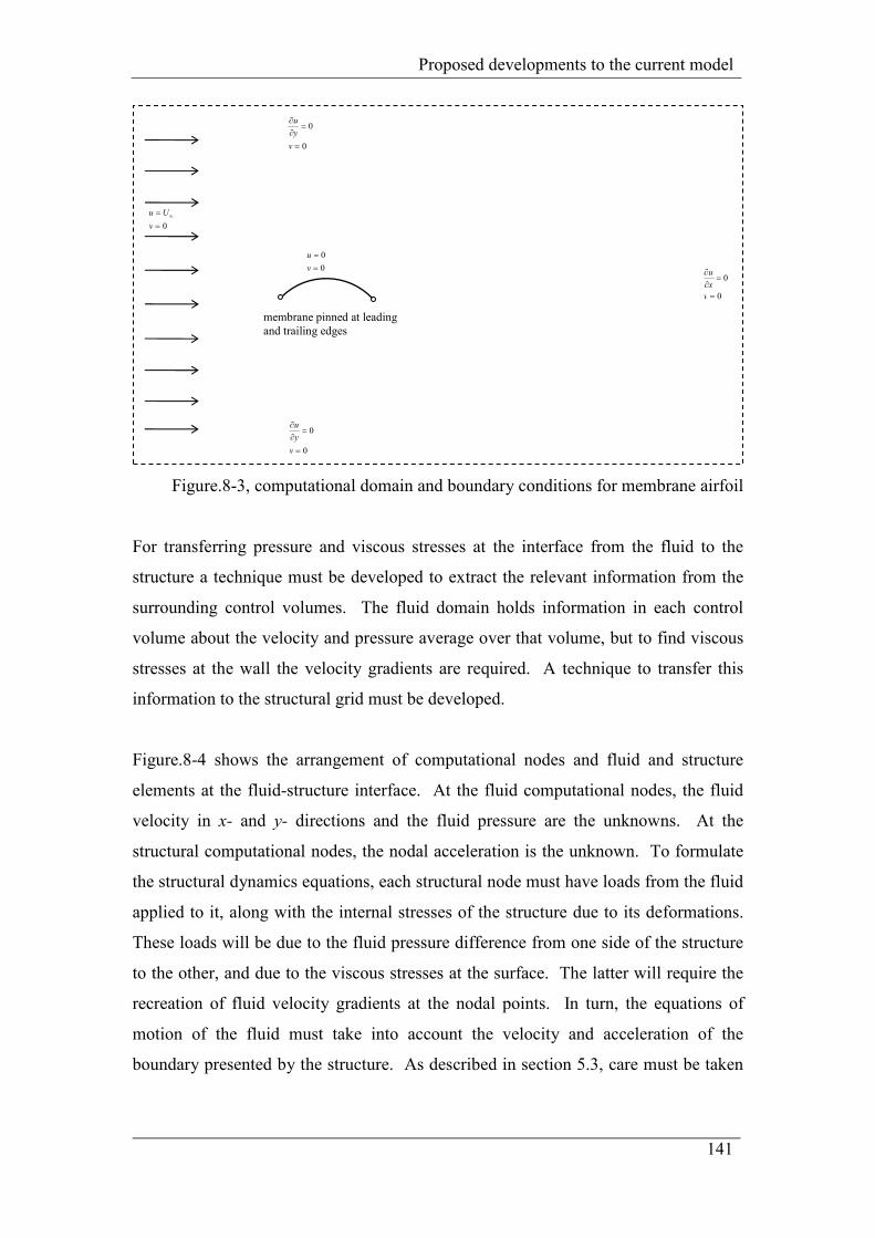
Proposed developments to the current model
141
Figure.8-3, computational domain and boundary conditions for membrane airfoil
For transferring pressure and viscous stresses at the interface from the fluid to the
structure a technique must be developed to extract the relevant information from the
surrounding control volumes. The fluid domain holds information in each control
volume about the velocity and pressure average over that volume, but to find viscous
stresses at the wall the velocity gradients are required. A technique to transfer this
information to the structural grid must be developed.
Figure.8-4 shows the arrangement of computational nodes and fluid and structure
elements at the fluid-structure interface. At the fluid computational nodes, the fluid
velocity in x- and y- directions and the fluid pressure are the unknowns. At the
structural computational nodes, the nodal acceleration is the unknown. To formulate
the structural dynamics equations, each structural node must have loads from the fluid
applied to it, along with the internal stresses of the structure due to its deformations.
These loads will be due to the fluid pressure difference from one side of the structure
to the other, and due to the viscous stresses at the surface. The latter will require the
recreation of fluid velocity gradients at the nodal points. In turn, the equations of
motion of the fluid must take into account the velocity and acceleration of the
boundary presented by the structure. As described in section 5.3, care must be taken
membrane pinned at leading
and trailing edges
0=
= ∞
v
Uu
0
0
=
=
v
u
0
0
=
=∂∂
v
y
u
0
0
=
=∂∂
v
y
u
0
0
=
=∂∂
v
x
u
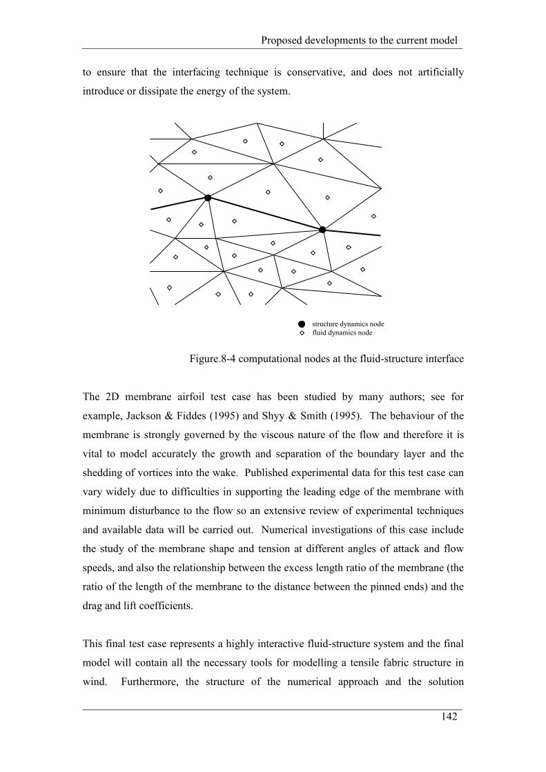
Proposed developments to the current model
142
to ensure that the interfacing technique is conservative, and does not artificially
introduce or dissipate the energy of the system.
Figure.8-4 computational nodes at the fluid-structure interface
The 2D membrane airfoil test case has been studied by many authors; see for
example, Jackson & Fiddes (1995) and Shyy & Smith (1995). The behaviour of the
membrane is strongly governed by the viscous nature of the flow and therefore it is
vital to model accurately the growth and separation of the boundary layer and the
shedding of vortices into the wake. Published experimental data for this test case can
vary widely due to difficulties in supporting the leading edge of the membrane with
minimum disturbance to the flow so an extensive review of experimental techniques
and available data will be carried out. Numerical investigations of this case include
the study of the membrane shape and tension at different angles of attack and flow
speeds, and also the relationship between the excess length ratio of the membrane (the
ratio of the length of the membrane to the distance between the pinned ends) and the
drag and lift coefficients.
This final test case represents a highly interactive fluid-structure system and the final
model will contain all the necessary tools for modelling a tensile fabric structure in
wind. Furthermore, the structure of the numerical approach and the solution
structure dynamics node
fluid dynamics node
Proposed developments to the current model
143
algorithm means that extension of the model to 3D problems would not require
changes in the solution approach as a whole and thus could be achieved with
relatively few alterations to the code. A 3D test case will be attempted if time allows.
A possible additional development would be the extension of the model to turbulent
flow, which again will be investigated if time allows.

References
9 References
Barnes (1977) ‘Form-finding and analysis of tension structures by dynamic
relaxation’, PhD thesis, University of London.
Barnes (1999) ‘Form finding and analysis of tension structures by dynamic
relaxation’, International Journal of Space Structures, v14 n2, pp89-104.
Barth & Jespersen (1989) ‘The design and application of upwind schemes on
unstructured meshes’, 27th Aerospace Sciences Meeting, 9-12 January, Reno, NV,
AIAA paper 89-0366.
Barton (1998) ‘Comparison of SIMPLE- and PISO- type algorithms for transient
flows’, International Journal for Numerical Methods in Fluids, v26 n4, pp459-483.
Batina (1989a) ‘Unsteady Euler airfoil solutions using unstructured dynamic
meshes’, 27th Aerospace Sciences Meeting, 9-12 January, Reno, NV, AIAA paper 89-
0115.
Batina (1989b) ‘Unsteady Euler algorithm with unstructured dynamic mesh for
comple-aircraft aeroelastic analysis’, Technical Papers Part 1, pp275-284, 30th
ASME/ASCE/AHS/ASC Structures, Structural Dynamics and Materials Conference,
3-5 April, Mobile, AL, AIAA paper 89-1189.
Batina (1990) ‘Unsteady Euler airfoil solutions using unstructured dynamic meshes’,
AIAA Journal, v28 n8, pp1381-1388.
Brooks & Hughes (1982) ‘Streamline upwind/Petrov-Galerkin formulations for
convection dominated flows with particular emphasis on the incompressible Navier-
Stokes equations’, Computer Methods in Applied Mechanics and Engineering, v32
n1-3, pp199-259.

References
Bunge, Rung & Thiele (2001) ‘A two-dimensional sail in turbulent flow’, 1st
International Conference on Fluid Structure Interaction, 26-28 September 2001,
Computational Mechanics Inc (pub.).
Chiandussi, Bugeda & Onate (2000) ‘A simple method for automatic update of finite
element meshes’, Communications in Numerical Methods in Engineering, v16 n1,
pp1-19.
Chorin (1967) ‘A numerical method for solving incompressible viscous flow
problems’, Journal of Computational Physics, v2 n1, pp12-26.
Chow, Cross & Pericleous (1996) ‘A natural extension of the conventional finite
volume method into polygonal unstructured meshes for CFD application’, Applied
Mathematical Modelling, v20 n2, pp170-183.
Chung (2002) ‘Computational Fluid Dynamics’ Cambridge University Press,
Cambridge, England.
Clements (1973) ‘An inviscid model of two-dimensional vortex shedding’, Journal of
Fluid Mechanics, v57 n2, pp321-336.
Cottet & Koumoutsakos (2000) ‘Vortex methods: theory and practice’, Cambridge
University Press, Cambridge, MA.
Cyr & Newman (1996) ‘Flow past two-dimensional membrane aerofoils with rear
separation’, Journal of Wind Engineering and Industrial Aerodynamics, v63 n1-3,
pp1-16.
Date (2005) ‘Solution of transport equations on unstructured meshes with cell-
centred colocated variables. Part I: Discretisation’, International Journal of Heat &
Mass Transfer, v48 n6, pp1117-1127.
References
Davidson (1996) ‘A pressure correction method for unstructured meshes with
arbitrary control volumes’, International Journal for Numerical Methods in Fluids,
v22 n4, 265-281.
Day (1965) ‘An introduction to dynamic relaxation’, The Engineer, v219 n5688,
pp218-221.
Degand & Farhat (2002) ‘A three-dimensional torsional spring analogy method for
unstructured dynamic meshes’, Computers & Structures, v80 n3-4, pp305-316.
Delaunay (1934) ‘Sur la sphere vide’, Bulletin of the Academy of Sciences of the
USSR VII, Classe Sci. Mat. Nat. 6 pp793-800.
Demirdzic & Peric (1990) ‘Finite volume method for prediction of fluid flow in
arbitrarily shaped domains with moving boundaries’, International Journal for
Numerical Methods in Fluids, v10 n7, pp771-790.
Djayapertapa, Allen & Fiddes (2001) ‘Two-dimensional transonic aeroservoelastic
computations in the time domain’, International Journal for Numerical Methods in
Engineering, v52 n12, 1355-1377.
Eriksson (1982) ‘Generation of boundary-conforming grids around wing-body
configurations using transfinite interpolation’, AIAA Journal, v20 n10, pp1313-1320.
Farhat, Geuzaine & Brown (2003) ‘Application of a three-field nonlinear fluid-
structure formulation to the prediction of the aeroelastic parameters of an F-16
fighter’, Computers & Fluids, v32 n1, pp3-29.
Farhat, Degand, Koobus & Lesoinne (1998), ‘Torsional springs for two-
dimensional dynamic unstructured fluid meshes’, Computer Methods in Applied
Mechanics and Engineering, v163 n1-4, pp231-245.
Farhat, Lesoinne, Stern & Lanteri (1997) ‘High performance solution of three-
dimensional nonlinear aeroelastic problems via parallel partitioned algorithms:
References
methodology and preliminary results’, Advances in Engineering Software, v28 n1,
pp43-61.
Farhat & Lin (1993) ‘A structure attached corotational fluid grid for transient
aeroelastic computations’, AIAA Journal, v31 n3, pp597-599.
Farnell, David & Barton (2004a) ‘Numerical simulations of a filament in a flowing
soap film’, International Journal for Numerical Methods in Fluids, v44 n3, pp313-330.
Farnell, David & Barton (2004b) ‘Coupled states of flapping flags’, Journal of
Fluids and Structures, v19 n1, pp29-36.
Ferziger & Peric (2002) ‘Computational Methods for Fluid Dynamics, 3rd edition’,
Springer-Verlag, Berlin, Germany.
Frink & Pirzadeh (1998) ‘Tetrahedral finite-volume solutions to the Navier-Stokes
equations on complex configurations’, 10th International Conference on Finite
Elements in Fluids, 5-8 January 1998, v31 n1, pp175-187, John Wiley & Sons.
Gingold & Monaghan (1977) ‘Smoothed particle hydrodynamics: theory and
applications to non-spherical stars’, Monthly Notices of the Royal Astronomical
Society, v181, pp375-389.
Gluck, Breuer, Durst, Halfmann & Rank (2001) ‘Computation of fluid-structure
interaction on lightweight structures’, J of Wind Engineering & Industrial
Aerodynamics, v89 n14-15, pp1351-1368.
Gluck, Breuer, Durst, Halfmann & Rank (2003) ‘Computation of wind-induced
vibrations of flexible shells and membranous structures’, Journal of Fluids and
Structures, v17 n5, pp739-765.
Gnoffo (1983) ‘A finite volume adaptive grid algorithm applied to planetary entry
flowfields’, AIAA Journal, v21 n9, pp1249-1254.
References
Guruswamy (2002) ‘A review of numerical fluids/structures interface methods for
computations using high-fidelity equations’, Computers & Structures, v80 n1, 31-41.
Hartel (1996) ‘Turbulent flows: direct numerical simulation and large-eddy
simulation’ in Peyred (ed.) ‘Handbook of Computational Fluid Dynamics’, Academic
Press, London.
Hartwich & Agrawal (1997) ‘Method for perturbing multiblock patched grids in
aeroelastic and design optimisation applications’, 13th AIAA Computational Fluid
Dynamics Conference, 29 June – 2 July, Snowmass Village, CO, Collection of
Technical Papers, Part 2, AIAA paper 97-2038.
Hodges & Pierce (2002) ‘Introduction to structural dynamics and aeroelasticity’,
Cambridge Aerospace Series, Cambridge University Press, Cambridge.
Holmes & Connel (1989) ‘Solution of the 2D Navier-Stokes equations on
unstructured adaptive grids’, 9th AIAA Computational Fluid Dynamics Conference,
13-15 July, Buffalo, NY, AIAA paper 89-1932.
Hubner, Walhorn & Dinkler (2004) ‘A monolithic approach to fluid-structure
interaction using space-time finite elements’, Computer Methods in Applied
Mehcanics and Engineering, v193 n23-26, pp2087-2104.
Jackson & Christie (1987) ‘Numerical analysis of three-dimensional elastic
membrane wings’, AIAA Journal, v25 n5, pp676-682.
Jackson & Fiddes (1995) ‘Two-Dimensional viscous flow past flexible sail sections
close to ideal incidence’, The Aeronautical Journal, v99 n986, pp217-225.
Johnson & Tezduyar (1996) ‘Simulation of multiple spheres falling in a liquid-filled
tube’, Computer Methods in Applied Mechanics and Engineering, v134 n3-4, pp351-
373.
References
Jones & Samareh-Abolhassani (1995) ‘A grid generation system for multi-
disciplinary design optimization’, Proceedings of the 12th AIAA Computational Fluid
Dynamics Conference, Part 1, pp 474-482, AIAA.
Kamakoti & Shyy (2004a) ‘Evaluation of geometric conservation law using
pressure-based fluid solver and moving grid technique’, International Journal of
Numerical Methods for Heat & Fluid Flow, v14 n7, pp849-863.
Kamakoti & Shyy (2004b) ‘Fluid-Structure interaction for aeroelastic applications’,
Progress in Aerospace Sciences, v40 n8, pp535-558.
von Kármán (1911) ‘Uber den mechanismus des widerstandes, den ein bewegter
Korper in einer Flussigkeit erzeugt’, in ‘Collected Works’, v1, pp339-358,
Butterworth, London, 1956.
Koomullil & Soni (1999) ‘Flow simulation using generalised static and dynamic
grids’, AIAA Journal, v37 n2, pp1551-1557.
Lamb (1993) ‘Hydrodynamics, 6th edition’, Cambridge University Press, Cambridge,
UK.
Le Tallec & Mouro (2001) ‘Fluid structure interaction with large structural
displacements’, Computer Methods in Applied Mechanics and Engineering, v190
n24-25, pp3039-3067.
Lian, Shyy, Ifu & Verron (2002) ‘A computational model for coupled membrane-
fluid dynamics’, 32nd AIAA Fluid Dynamics Conference & Exhibit, 34-36 June 2002,
AIAA paper 2002-2972.
Lian, Steen, Trygg-Wilander & Shyy (2003) ‘Low Reynolds number turbulent flows
around a dynamically shaped airfoil’, Computers & Fluids, v32 n3, pp287-303.
Lin, Vezza & Galbraith (1997) ‘Discrete vortex method for simulating unsteady flow
around pitching aerofoils’, AIAA Journal, v35 n3, 494-499.
References
Liu, Cai, Zhu, Tsai & Wong (2001) ‘Calculation of wing flutter by a coupled fluid-
structure method’, Journal of Aircraft, v38 n2, pp334-342.
Loeb (1934) ‘The Kinetic Theory of Gases, 2nd edition’, The McGraw Hill Book
Company.
Lohner, Yang, Cebral, Baum, Luo, Pelessone & Charman (1995) ‘Fluid-structure
interaction using a loose coupling algorithm and adaptive unstructured grids’, in
Hafez & Oshima (eds.) ‘Computational Fluid Dynamics Review 1995’, John Wiley &
Sons, Chichester, England.
Lucy (1977) ‘A numerical approach to the testing of the fission hypothesis’,
Astronomical Journal, v82 n12, pp 1013-1024.
Masud (1993) ‘A space-time finite element method for fluid-structure interaction’,
PhD dissertation, Stanford University.
McBride, Croft & Cross (2003) ‘Combined vertex-based - cell-centred finite volume
method for flows in complex geometries’, 3rd International conference on CFD in the
Minerals and Process Industries, 10-12 December 2003, CSIRO (pub.).
Mestreau & Lohner (1996) ‘Airbag simulation using fluid/structure coupling’, 34th
Aerospace Sciences Meeting & Exhibit, AIAA paper 96-0798.
Michler, Hulshoff, van Brummelen & de Borst (2004) ‘A monolithic approach to
fluid-structure interaction’, Computers & Fluids, v33 n5-6, pp839-848.
Monaghan (1992) ‘Smoothed particle hydrodynamics’, Annual Review of
Astronomy and Astrophysics, v30, pp543-547.
Morand & Ohayon (1995) ‘Fluid structure interaction, applied numerical methods’,
John Wiley & Sons Ltd, Chichester.
References
Muzaferija (1994) ‘Adaptive finite volume method for flow predictions using
unstructured meshes and multigrid approach’, PhD thesis, University of London
Najjar & Balachandar (1998) ‘Low-frequency unsteadiness in the wake of a normal
flat plate’, Journal of Fluid Mechanics, v370, pp101-147.
Namkoong, Choi & Yoo (2005) ‘Computation of dynamic fluid-structure interaction
in two-dimensional laminar flows using combined formulation’, Journal of Fluids and
Structures, v20 n1, pp51-69.
Newman (1987) ‘Aerodynamic theory for membranes and sails’, Progress in
Aerospace Sciences, v24 n1, pp1-27.
Ng & Siauw (2001) ‘Unsteady viscous flow model on moving the domain through a
stenotic artery’, Proceedings of the Institution of Mechanical Engineers, Part H:
Journal of Engineering in Medicine, v215 n2, pp237-249.
Oh, Kim & Kwon (2003) ‘Time-accurate Navier-Stokes simulation of vortex
convection using an unstructured dynamic mesh proceedure’, Computers & Fluids,
v32 n5, pp727-749.
Otto (1971) ‘Tensile structures’, MIT Press, Cambridge, MA.
Palmerio (1994) ‘An attraction-repulsion mesh adaptation model for flow solution on
unstructured grids’, Computers and Fluids, v23 n3, pp487-506.
Pan & Cheng (1993) ‘Upwind finite-volume Navier-Stokes computations on
unstructured triangular meshes’, AIAA Journal, v31 n9, pp1618-1625.
Patankar & Spalding (1979) ‘A calculation procedure for heat, mass and
momentum transfer in three-dimensional parabolic flows’, International Journal of
Heat & Mass Transfer, v15, pp1787-1806.

References
Perez-Segarra, Oliva & Consul (1996) ‘Analysis of some numerical aspects in the
solution of the Navier-Stokes equations using non-orthogonal colocated finite volume
methods’, Proceedings of the 1996 3rd ECOMAS CFD conference, 9-13 September.
Peric, Kessler & Scheuerer (1998) ‘Comparison of finite-volume numerical methods
with staggered and colocated grids’, Computers & Fluids, v16 n4, 389-403.
Prabhakara & Deshpande (2004) ‘The no-slip boundary condition in fluid
mechanics’, Resonance – Journal of Science Education, v9 n4, pp50-92.
Rausch, Batina & Yang (1989) ‘Euler flutter analysis of airfoils using unstructured
dynamic meshes’, AIAA paper 89-1384.
Reuther, Jameson, Farmer, Martinelli & Saunders (1996) ‘Aerodynamic shape
optimization of complex aircraft configurations via an adjoint formulation’, 34th
Aerospace Sciences Meeting and Exhibit, 15-18 January, Reno, NV, AIAA paper 96-
0094.
Rhie & Chow (1983) ‘Numerical study of the turbulent flow past an airfoil with
trailing edge separation’, AIAA Journal, v21 n11, pp1525-1532.
Robinson, Batina & Yang (1991) ‘Aeroelastic analysis of wings using the Euler
equations with a deforming mesh’, Journal of Aircraft, v28 n10, pp781-788.
Schoop, Besser & Taenzer (1998) ‘On the elastic membrane in a potential flow’,
International Journal for Numerical Methods in Engineering, v41 n2, pp271-291.
Schuster, Liu & Hussel (2003) ‘Computational aeroelasticity: success, progress,
challeng’, Journal of Aircraft, v40 n5, pp843-856.
Shyy & Smith (1995) ‘Computation of Laminar Flow and Flexible Structure
Interaction’, in Hafez & Oshima (eds.) ‘Computational Fluid Dynamics Review
1995’, John Wiley & Sons, Chichester, England.
References
Singh, Newman & Baysal (1995) ‘Dynamic unstructured method for flows past
multiple objects in relative motion’, AIAA Journal, v33 n4, pp641-649.
Smith, Hodges & Cesnik (2000) ‘Evaluation of computational algorithms suitable
for fluid-structure interactions’, Journal of Aircraft, v37 n2, pp282-294.
Smith & Shyy (1996) ‘Computation of aerodynamic coefficients for a flexible
membrane airfoil in turbulent flow: A comparison with classical theory’, Physics of
Fluids, v8 n12, pp3345-3353.
Stein (1999) ‘Simulation and modelling techniques for parachute fluid-structure
interactions’, PhD dissertation, University of Minnesota.
Stein, Benney, Kalro, Tezduyar, Bretl & Potvin (1999) ‘Fluid-structure interaction
simulations of a cross parachute: Comparisons of numerical predictions with wind
tunnel data’, proceedings of the Confederation of European Aerospace
Societies/AIAA 15th Aerodynamic Decelerator Systems Technology Conference,
AIAA paper 99-1725, pp172-181.
Stein, Benney, Tezduyar, Leonard & Accorsi (2001) ‘Fluid-structure interactions
of a round parachute: modelling and simulation techniques’, Journal of Aircraft, v38
n5, pp800-808.
Stein, Tezduyar & Benney (2003) ‘Mesh moving techniques for fluid-structure
interactions with large displacements’, Journal of Applied Mechanics, v70 n1, pp58-
63.
Stein, Tezduyar, Kumar, Sathe, Benney & Charles (2004) ‘Numerical simulation
of soft landing for clusters of cargo parachutes’, in Neittaanmaki, Rossi, Korotov,
Onate, Periaux & Knorzer (ed.s) proceedings of European Congress on
Computational Methods in Applied Sciences and Engineering 2004, Jyvaskyla, 24-28
July.
References
Sweeney & Meshell (2003) ‘Fast numerical simulation of vortex shedding in tube
arrays using a discrete vortex method’, Journal of Fluids and Structures, v18 n5,
pp501-512.
Tamaddon-Jahromi, Townsend & Webster (1994) ‘Unsteady viscous flow past a
flat plate orthogonal to the flow’, Computers and Fluids, v23 n2, pp433-446.
Taniguchi & Kobayashi (1991) ‘Finite volume method on the unstructured grid
system’, Computers & Fluids, v19 n3-4, pp287-295.
Thomas & Lombard (1979) ‘Geometric conservation law and its application to flow
computations on moving grids’, AIAA Journal, v17 n10, pp1030-1037.
Tenekes & Lumley (1972) ‘A first course in turbulence’, The MIT Press, Cambridge,
Massachusetts, USA.
Tezduyar (1991) ‘Stabilised finite element formulations for incompressible flow
computations’, Advances in Applied Mechanics, v28, pp1-44.
Tezduyar, Behr & Liou (1992) ‘A new strategy for finite element computations
involving moving boundaries and interfaces – the deforming-spatial-domain/space-
time procedure: I. The concept and the preliminary tests’, Computer Methods in
Applied Mechanics and Engineering, v94 n6, pp339-351.
Tezduyar, Behr, Mittal & Johnson (1992) ‘Computation of unsteady
incompressible flows with the finite element methods – space-time formulations,
iterative strategies and massively parallel implementations’, in Smolinski, Liu,
Hulbert & Tamma (eds), ‘New Methods in Transient Analysis’, v143, pp7-24, ASME,
New York.
Tezduyar & Osawa (1999) ‘Methods for parallel computation of complex flow
problems’, Parallel Computing, v25 n13-14, pp2039-2066.
References
Tezduyar & Osawa (2001a) ‘The multi-domain method for computation of the
aerodynamics of a parachute crossing the far wake of an aircraft’, Computer
Methods in Applied Mechanics and Engineering, v191 n6-7, pp705-716.
Tezduyar & Osawa (2001b) ‘Fluid-structure interactions of a parachute crossing
the far wake of an aircraft’, Computer Methods in Applied Mechanics and
Engineering, v191 n6-7, pp717-726.
Tsai, Wong, Cai, Zhu & Liu (2001) ‘Unsteady flow calculations with a parallel
multiblock moving mesh algorithm’, AIAA Journal, v39 n6, pp1021-1029.
Venkatakrishnan & Mavriplis (1996) ‘Implicit method for the computation of
unsteady flows on unstructured grids’, Journal of Computational Physics, v127 n2,
pp380-397.
Versteeg & Malalasekera (1995) ‘An introduction to computational fluid dynamics –
the finite volume method’, Prentice Hall, Harlow, England.
Wakefield (1999) ‘Engineering analysis of tension structures: theory and practice’,
Engineering Structures, v21 n8, pp680-690.
Xu & Accorsi (2004) ‘Finite element mesh update methods for fluid-structure
interaction simulations’, Finite Elements in Analysis and Design, v40 n9-10, 1259-
1269.
Zhang, Childress, Libchaber & Shelley (2000) ‘Flexible filaments in a flowing
soap film as a model for one-dimensional flags in a two-dimensional wind’, Nature,
v408 n6814, pp835-839.