Embed Size (px)
Citation preview
HAL Id: tel-00978589https://tel.archives-ouvertes.fr/tel-00978589
Submitted on 14 Apr 2014
HAL is a multi-disciplinary open accessarchive for the deposit and dissemination of sci-entific research documents, whether they are pub-lished or not. The documents may come fromteaching and research institutions in France orabroad, or from public or private research centers.
L’archive ouverte pluridisciplinaire HAL, estdestinée au dépôt et à la diffusion de documentsscientifiques de niveau recherche, publiés ou non,émanant des établissements d’enseignement et derecherche français ou étrangers, des laboratoirespublics ou privés.
NUMERICAL MODELLING OF EROSION OF ACOHESIVE SOIL BY A TURBULENT FLOW
F. Mercier
To cite this version:F. Mercier. NUMERICAL MODELLING OF EROSION OF A COHESIVE SOIL BY A TURBU-LENT FLOW. Fluids mechanics [physics.class-ph]. Aix-Marseille Université, 2013. English. <tel-00978589>
UNIVERSITY OF AIX-MARSEILLE DOCTORAL SCHOOL: ENGINEERING SCIENCES
NUMERICAL MODELLING OF EROSION OF A
COHESIVE SOIL BY A TURBULENT FLOW
PhD Thesis presented to obtain the grade of
DOCTOR OF THE UNIVERSITY OF AIX-MARSEILLE
SPECIALITY: MECHANICS AND PHYSICS OF FLUIDS
by
Fabienne MERCIER
Defended publicly on 11 June 2013
Before a jury composed of Fabien ANSELMET IRPHE Co-thesis supervisor Eric BARTHÉLÉMY LEGI Examiner Stéphane BONELLI IRSTEA Thesis supervisor Roland BORGHI ECM Examiner Jean-Robert COURIVAUD EDF-CIH Guest Jean-Jacques FRY EDF-CIH Guest Frédéric GOLAY IMATH Examiner Philippe GONDRET FAST Reporter Didier MAROT GeM Reporter Marc MÉDALE IUSTI Examiner Patrick PINETTES geophyConsult Guest

MODELLING THE EROSION OF A COHESIVE SOIL BY A TURBULENT FLOW
2
ACKNOWLEDGEMENTS
3
I would first like to thank my thesis supervisors, Stéphane BONELLI and Fabien ANSELMET. Their sceintific expertise and the knowledge they provided allowed me to carry out this complex study at the crossroads of several disciplines in an pleasant atmosphere. I would also like to thank the manager of geophyConsult, the company involved in the CIFRE funding (Industrial Research Convention: PhD conducted with an industrial partnership), Patrick PINETTES, for his technical and scientific competences, and for his constant moral support. The organisation of this CIFRE thesis would certainly never have succeeded without the contribution of Jean-Jacques FRY. Thank you for all the advice that you gave me at the beginning of this adventure and afterwards. I also thank Jean-Robert COURIVAUD, first for the funding given by EDF for this thesis and for his continuous follow-up of my work and his scientific contribution to this study. I would also like to thank Laurent PEYRAS for his active contribution to the organisation of this thesis and his support throughout this study. My thanks also go to Pierre PHILIPPE, Frédéric GOLAY and Roland BORGHI for their availability and encouragement. I thank the members of the jury for the attention they have given to my work and the resulting positive feedback. Your questions and remarks contributed to the subsequent direction taken for work performed in the framework of this thesis. I thank the entire team of the Laboratoire de Mécanique des Sols de l’Unité des Ouvrages hydrauliques et Hydrologie of IRSTEA. I thank Alain BERNARD and Nadia BENAHMED for their perspicacious advice. I thank Faustine BYRON, Yves GREMEAUX and Guillaume NUNES for their technical assistance, their good humour and all the good times we spent together. I thank my fellow PhD students who contributed to the good atmosphere in the team on a daily basis: Caroline ZANETTI, Mohammed ARIS, Félix BONNET, Kien NGUYEN, Jeff NGOMA and Zhenzhen LIU. I am also very grateful to my office colleagues, Damien LACHOUETTE, Marc VUILLET, Ismail FAKHFAKH, Marika BOUTRY and particularly Li-Hua LUU, who was kind enough to read this thesis. My thanks also go to the assistants of the unit and the group: Martine SYLVESTRE, Monique COSTET, Christiane BONNET and Dominique BREIL. I spare a thought for all the other people in the IRSTEA team that I have frequented during different sports and summer activities. I especially thank the members of the computer department of the IRSTEA centre of Aix-en-Provence: Alain GERARD, Mathieu LESTRADE and Etienne BLANC. I would also like to thank Vincent CHEVALLEREAU and Gérard DELANCE as well as the whole team of the IRSTEA calculation unit, for the resources that they implemented for me so I could carry out my scientific calculation projects. I also extend my thanks to the Information Systems Division (DSI) of IRSTEA.

ACKNOWLEDGEMENTS
4
I am grateful to my colleagues of geophyConsult : Cyril GUIDOUX, Rémi BEGIN, Olivier MARIN and above all Clément MORAS, for all the JET tests he performed with me or for my research. I am also grateful to the IRPHE team, especially Muriel AMIELH, and to Pascal CAMPION of ED353 for his availability and efficiency. And above all, I am especially grateful to my family and friends without whom none of this would have been possible.
5
TABLE OF CONTENTS
Figure captions ................................................................................................................... 9 Table captions .................................................................................................................... 15 Nomenclature ..................................................................................................................... 17 Introduction ........................................................................................................................ 23 Chapter 1. State of the art ............................................................................................... 27
1.1 Erosion in hydraulic structures ............................................................................ 27 1.1.1 Context ....................................................................................................... 27
1.1.1.1 Erosion at the scale of the structure................................................ 27 1.1.1.2 Estimation of soil erodibility .......................................................... 29 1.1.1.3 Erosion parameters ......................................................................... 29
1.1.2 HET and JET erosion tests ......................................................................... 30 1.1.2.1 The Hole Erosion Test .................................................................... 30 1.1.2.2 The Jet Erosion Test ....................................................................... 33
1.1.3 Erosion laws ............................................................................................... 35 1.1.3.1 Rate of soil removal ....................................................................... 35 1.1.3.2 Determination of critical shear stress ............................................. 39 1.1.3.3 Correlation of erosion coefficient and critical shear stress ............ 41
1.2 Numerical modelling of erosion .......................................................................... 42 1.2.1 Context ....................................................................................................... 42
1.2.1.1 Erosion of granular soils and cohesive soils .................................. 42 1.2.1.2 Different approaches to model interfaces ....................................... 43
1.2.2 Biphasic and triphasic models .................................................................... 44 1.2.2.1 The approach of Papamichos and Vardoulakis (2005) .................. 44 1.2.2.2 The approach of Ouriemi et al. 2009 .............................................. 45
1.2.3 Singular interface ....................................................................................... 46
1.3 Conclusions on the state of the art ...................................................................... 48 Chapter 2. Modelling method ......................................................................................... 51
2.1 Hypotheses .......................................................................................................... 51 2.1.1 Single phase modelling and slow erosion kinetics ..................................... 51 2.1.2 Analysis of orders of magnitude ................................................................ 52
2.2 Flow modelling ................................................................................................... 53 2.2.1 RANS modelling and the closure problem ................................................. 53
2.2.1.1 Navier-Stokes Equations ................................................................ 53 2.2.1.2 Resolution by DNS or LES ............................................................ 53 2.2.1.3 Choice of RANS models ................................................................ 53
2.2.2 Turbulence models ..................................................................................... 54 2.2.2.1 Eddy viscosity models .................................................................... 54 2.2.2.2 Reynolds Stress Model ................................................................... 55
TABLE OF CONTENTS
6
2.3 Erosion modelling ............................................................................................... 56
2.3.1 Classical erosion law .................................................................................. 56 2.3.1.1 Definition of the eroded mass flux ................................................. 56 2.3.1.2 Shear stress ..................................................................................... 56
2.3.2 The standard erosion law adapted to impinging jets .................................. 57 2.3.2.1 Geometric singularity induced by the erosion law ......................... 57 2.3.2.2 Smoothing of the non eroded soil peak .......................................... 58 2.3.2.3 Adaptation of the erosion law ........................................................ 60
2.4 Numerical model ................................................................................................. 61
2.4.1 Global numerical method ........................................................................... 61 2.4.2 Flow discretization ..................................................................................... 62
2.4.2.1 Solution of Navier-Stokes equations .............................................. 62 2.4.2.2 Wall laws ........................................................................................ 63 2.4.2.3 Taking roughness into account ....................................................... 65
2.4.3 Updating the position of the interface ........................................................ 66 2.4.3.1 Interface displacement code ........................................................... 66 2.4.3.2 Remeshing ...................................................................................... 68
2.5 Conclusions on the modelling method ................................................................ 71
Chapter 3. Results obtained on impinging flows ........................................................... 73
3.1 Independency of results regarding mesh density and turbulence models ........ 73 3.1.1 Independency of results in relation to the meshing .................................... 74 3.1.2 Influence of the turbulence model .............................................................. 77
3.2 Erosion modelling ............................................................................................ 81 3.2.1 Comparison of results of the semi-empirical model ................................... 81 3.2.2 Study of the sensitivity of the model to erosion parameters ...................... 87 3.2.3 Discussion ................................................................................................... 93
3.3 Validation of the JET interpretation model ...................................................... 95 3.3.1 Characterization of the soils tested ............................................................. 95 3.3.2 JET modelling results ................................................................................. 101 3.3.3 Discussion ................................................................................................... 107
3.4 Conclusions on the application to jet flows ...................................................... 108
Chapter 4. Results obtained on tangential flows ........................................................... 111
4.1 Validation of the numerical model in a 2D Poiseuille flow configuration ....... 111 4.1.1 Theoretical solution .................................................................................... 111 4.1.2 Numerical results ........................................................................................ 112
4.2 Concentrated leak erosion in turbulent flow .................................................... 114 4.2.1 Independence from meshing and turbulence models ................................. 115
4.2.1.1 Independence of results from mesh density ................................... 115 4.2.1.2 Influence of the turbulence model .................................................. 117
TABLE OF CONTENTS
7
4.2.2 Results with erosion ................................................................................... 120 4.2.3 Study of the model’s sensitivity to erosion parameters .............................. 126 4.2.4 Discussion ................................................................................................... 129
4.3 Modelling the HETs ......................................................................................... 130 4.3.1 Characterisation of the soils modelled ....................................................... 130 4.3.2 HET modelling results ................................................................................ 134 4.3.3 Discussion ................................................................................................... 142
4.4 Conclusions of the application to piping flows ................................................ 143
Chapter 5. Study of the erosion law ................................................................................ 145
5.1 Differences between JET and HET for erosion parameters ............................. 145 5.1.1 Experimental and literature data ................................................................. 145 5.1.2 Dispersion of results ................................................................................... 149 5.1.3 Influence of flow parameters ...................................................................... 151
5.2 Variables susceptible to influence erosion ....................................................... 153 5.2.1 Possible explanations for JET and HET differences? ................................ 153 5.2.2 Flow signature ............................................................................................ 155
5.2.2.1 Stresses and forces exerted by the flow on the plane ..................... 158 5.2.2.2 Pressure gradient ............................................................................ 160 5.2.2.3 Turbulence variables ...................................................................... 162
5.2.3 Flow variables susceptible to influence erosion ......................................... 164
5.3 Paths for developing the erosion law ................................................................ 166 5.3.1 Flow variables of the JET and HETs .......................................................... 166 5.3.2 Taking fluctuations into account in the stagnation region .......................... 171 5.3.3 Taking into account the pressure gradient in the erosion law .................... 172
5.4 Conclusions on the study of the erosion law .................................................... 173
Conclusion .......................................................................................................................... 175 Outlook for further research ............................................................................................... 179 References .......................................................................................................................... 181

TABLE OF CONTENTS
8
9
FIGURE CAPTIONS
Figure 1.1. Breach caused by flooding of the Virdourle river in 2002 (left) and breach of Teton Dam, 1976 (right). Figure 1.2. Simplified schematic diagram of the Hole Erosion Test. Figure 1.3. Photograph of the Hole Erosion Test experimental device. Figure 1.4. Grouping of HET test results for a flow rate imposed on the master curve defined by equation (1.7) of [Bonelli et al. 2012]. Figure 1.5. Simplified schematic diagram of the Jet Erosion Test. Figure 1.6. Photograph of experimental JET device in the laboratory and in-situ. Figure 1.7. Erosion rate as a function of shear stress, [Benahmed et al. 2012]. Figure 1.8. Influence of the critical shear stress on the erosion coefficient [Fell et al. 2013]. Figure 2.1. Shear stress profile for a normal flow and theoretical shape of the erosion figure for a so-called standard erosion law. Figure 2.2. Illustration of standard erosion figures obtained after Jet Erosion Tests (C. Moras - geophyConsult). Figure 2.3. Illustration of the pulsation of an axisymmetric jet in 3-D geometry [Hadziabdic and Hanjalic 2008]. Figure 2.4. Illustration of the displacement of the jet stagnation point: instantaneous velocities just above the plane of impingement of the jet at different times [Hadziabdic and Hanjalic 2008]. Figure 2.5. Scheme of the sequential uncoupled erosion model. Figure 2.6. Subdivisions of regions located close to the wall [Ansys 2009], with u* noted
τU
the friction velocity and *Py y uρ µ+ = the dimensionless distance from the centre of the first
cell to the wall. Figure 2.7. Shape of the mesh before (left) and after (right) a macro-remeshing. Example taken from the modelling of erosion due to a Poiseuille flow (cf. paragraph 4.1). Figure 2.8. Shape of the mesh at the beginning (left) and at the end of the erosion process (right) for the JET performed on soil C (cf. paragraph 3.3). Figure 2.9. Automation of erosion test models. Figure 3.1. Geometry and meshing developed for modelling the JETs. Figure 3.2. Refinement of the mesh in the JET configuration. Figure 3.3. Independence of the results in relation to mesh density, the shear stress on the water/soil interface before erosion begins, with the k-ω turbulence model. Figure 3.4. Independence of the results in relation to mesh density, pressure field on the water/soil interface before erosion begins, with the k-ω turbulence model. Figure 3.5. Comparison of turbulence models with bibliographical results, velocity field on the jet centreline. Figure 3.6. Comparison of turbulence models with bibliographical results: pressure field on the water/soil interface.
FIGURE CAPTIONS
10
Figure 3.7. Comparison of turbulence models with bibliographical results: shear stress on the water/soil interface. Figure 3.8. Velocity field as a function of time in the case of model k-ω above and in the case of model k-ε below. Figure 3.9. Evolution of the water/soil interface as a function of time, seen in the upper graph in the case of model k-ω and in the lower one for the k-ε model. Figure 3.10. Evolution of scour depth as a function of time. Comparison of numerical results and [Hanson and Cook 2004] model. Figure 3.11. Evolution of maximum shear stress as a function of scour depth at different times for models k-ε and k-ω in comparison to the results of the model of [Hanson and Cook 2004]. Figure 3.12. Evolution of the velocity field on the jet centreline, model k-ω. Figure 3.13. Evolution of shear stress on the water/soil interface as a function of time, model k-ω. Figure 3.14. Evolution of the pressure field on the water/soil interface as a function of time, model k-ω. Figure 3.15. Evolution of the pressure field as a function of time. The results obtained with the k-ω model shown above and with the k-ε model shown below. Only the values lower than 10% of the full spectrum are shown. Figure 3.16. Parametric study of the influence of the critical shear stress on the evolution of scour depth as a function of time for the turbulence model k-ω with kd =10-5 m².s/kg. Figure 3.17. Parametric study of the influence of critical shear stress on the evolution of scour depth as a function of time for the turbulence model k-ω, τc=11 Pa or τc=9 Pa. Figure 3.18. Velocity fields relative to the parametric study at times t = 6 s, t = 200 s, t = 600 s and t = 15000 s, model k-ω. Figure 3.19. Parametric study, evolution of the maximum shear stress as a function of scour depth at different times. Figure 3.20. Maximum scour depth as a function of the critical shear stress , model k-ω, kd
=10-5 m².s/kg. Figure 3.21. Time in which the depth of the cavity has reached half the final depth, plotted as a function of the erosion kinetics coefficient, τc=11 Pa, model k-ω. Figure 3.22. Time for which the depth of the cavity has reached half of the final depth plotted as a function of shear stress, kd =10-5 m².s/kg, model k-ω. Figure 3.23. Granulometric curves of materials A and B. Figure 3.24. Position of soils A, B and C in the classification of [Hanson and Simon 2001]. Figure 3.25. Photographs of soil samples before (left) and after (right) JETs, with from top to bottom images corresponding to soils A, B and C, respectively. Figure 3.26. Evolution of the scour depth for tests performed on soils A, B and C, with the comparison of experimental data and the results of the semi-empirical model. Figure 3.27. Comparison of numerical results for turbulence models k-ω and k-ε, with the experimental and semi-empirical results for the test on soil B. Figure 3.28. Comparison of numerical results for turbulence models k-ω and k-ε, with the experimental and semi-empirical results for the test on soil C.
FIGURE CAPTIONS
11
Figure 3.29. Evolution of the soil/water interface as a function of time with, from top to bottom, graphs corresponding to the tests performed on soils A, B and C, model k-ω. Figure 3.30. Shape of the erosion figures obtained numerically, bounded by the mould (black line) in which the tests were performed on soils A, B and C, model k-ω. Figure 3.31. Comparison of erosion figures found for the test performed on soil A numerically and experimentally. Graph bounded by the outline of the mould (black line), model k-ω. Figure 3.32. Evolution of the shear stress on the soil/water interface as a function of time with, from top to bottom, graphs corresponding to the tests performed on soils A, B and C, model k-ω. Figure 3.33. Shear stresses on the water/soil interface at the initial time and critical shear stresses, for soils A, B and C, model k-ω. Figure 3.34. Shear stress evolution for the three tests as a function of scour depth, model k-ω. Figure 3.35. Velocity fields and profiles of the soil/water interface as a function of time with, from top to bottom, results obtained for materials A, B and C, model k-ω. Figure 4.1. Schematic diagram of modelling the erosion of a channel by laminar flow. Figure 4.2. Velocity profiles at the pipe inlet as a function of time. Figure 4.3. Velocity fields at different times, with a 1 cm length pipe. Figure 4.4. Pipe diameter as a function of dimensionless time. Comparison of numerical and theoretical results. Figure 4.5. Geometry and shape of the mesh used to model the HETs. Figure 4.6. Results independency regarding mesh density, the mean velocity field on the axis of symmetry before erosion begins, for the k-ε turbulence model. Figure 4.7. Independence of the results from the mesh density, with shear stress on the water/soil interface before erosion begins, for the k-ε turbulence model. Figure 4.8. Comparison of the influence of the turbulence model for the velocity field on the axis of symmetry and for the mean velocity according to axis r
.
Figure 4.9. Comparison of the influence of the turbulence model for the pressure inside the pipe at the erodible walls. Figure 4.10. Comparison of the influence of the turbulence model for the shear stress on the water/soil interface. Figure 4.11. Evolution of the velocity field and the erosion figure as a function of time. Figure 4.12. Evolution of the profile of the water/soil interface as a function of time. Figure 4.13. Evolution of the velocity field on the axis of symmetry as a function of time. Figure 4.14. Evolution of shear stress on the water/soil interface as a function of time. Figure 4.15. Evolution of the pressure field on the water/soil interface as a function of time. Figure 4.16. Evolution of the pressure differential along the useful length. Comparison of the numerical results with Bonelli’s model [Bonelli et al. 2006]. Figure 4.17. Evolution of the shear stress in 6 cmx = , comparison of the numerical results with [Bonelli et al. 2006] model. Figure 4.18. Evolution of the radius of the pipe diameter. Comparison of the numerical results and the model of [Bonelli et al. 2006].
FIGURE CAPTIONS
12
Figure 4.19. Evolution of the pressure differential between sections A and B. Comparison of the experimental and numerical results and those given by the model of [Bonelli et al. 2006]. Figure 4.20. Evolution of the pressure differential between sections A and B. Comparison of the results of the parametric study and the experimental data. Figure 4.21. Evolution of the pipe diameter 6 cmx = as a function of time, results of the parametric study. Figure 4.22. Pipe radius 6 cmx = at the end of the erosion process. Comparison of the numerical results given by the model of [Bonelli et al. 2006]. Figure 4.23. Illustration of the erosion kinetics as a function of the erosion coefficient. Comparison of the numerical results and the model of [Bonelli et al. 2006]. Figure 4.24. Illustration of erosion kinetics as a function of critical shear stress, comparison of numerical results and the model of [Bonelli et al. 2006]. Figure 4.25. Granulometric curves of white kaolinite, proclay kaolinite and Hostun sand [Benahmed and Bonelli 2012]. Figure 4.26. Classification of soils tested with the HET in the classification of [Wan and Fell 2004], soil A, ∆ soil D and soil E. Figure 4.27. Evolution of the pressure differential between sections A and B for the tests performed on soils A, D and E, comparison of experimental data with the results of the analytical model. Figure 4.28. Photographs of soil samples before (left) and after (right) the HET tests, with, from top to bottom images corresponding to the soils A, D and E, respectively (F. Byron, IRSTEA). Figure 4.29. Comparison of numerical, experimental and semi-empirical results for the HET on soil A. Figure 4.30. Comparison of numerical, experimental and semi-empirical results for the HET on soil D. Figure 4.31. Comparison of numerical, experimental and semi-empirical results for the HET on soil E. Figure 4.32. Evolution of the water/soil interface as a function of time with, from top to bottom, the graphs corresponding to the tests performed on soils D and E. Figure 4.33. Shape of the scour holes found numerically, comparison of the results obtained for the tests performed on soils A, D and E. Figure 4.34. Illustration of typical profiles of scour holes obtained following the HETs (F. Byron, IRSTEA). Figure 4.35. Evolution of velocity fields and the erosion figure at the end of the erosion process, with, from top to bottom the results obtained for the tests carried out on soils A, D and E. Figure 4.36. Evolution of shear stress at the water/soil interface as a function of time, with from top to bottom the graphs corresponding to the tests carried out on soils D and E. Figure 4.37. Shear stresses on the water/soil interface at the initial time and critical shear stresses for soils A, D and E. Figure 4.38. Evolution of shear stress for the three tests as a function of the radius reached. Values taken in the middle of the erodible pipe.
FIGURE CAPTIONS
13
Figure 4.39. Evolution of shear stress for the test on soil A as a function of the radius reached. Values taken in x = 6 cm. Figure 5.1. Erosion coefficient obtained with the JET as a function of the erosion coefficient obtained with the HET. Figure 5.2. Critical shear stress obtained with the HET as a function of the critical shear stress found with the JET. Figure 5.3. Ratio of the critical shear stresses obtained for the HET and JET as a function of the water content of the materials tested. Figure 5.4. Erosion parameters obtained following the test campaign on soil F. Figure 5.5. Erosion parameters obtained following the tests on the clay/sand mixture. Figure 5.6. Comparison of results obtained for repeatability tests on soil F, experimentally and using the semi-empirical model of [Hanson and Cook 2004]. Figure 5.7. Critical shear stress as a function of the hydraulic head applied, soil F, 0 6 cm=z . Figure 5.8. Critical shear stress as a function of jet nozzle/soil distance, soil F, 172 cm∆ =H . Figure 5.9. Erosion rate as a function of shear stress. Comparison of experimental results and the JET and HET interpretation models for soil A. Figure 5.10. Schematic representation of the flow configuration. Figure 5.11. Velocity field as a function of the inclined plane, for 90°, 135° and 180°. Figure 5.12. Vertical velocity profiles above the fixed plane as a function of the inclined plane angle, for 90°, 135° and 180°. Figure 5.13. Results obtained for the pressure on the horizontal plane as a function of the inclined plane angle. Figure 5.14. Results obtained for the shear stress on the horizontal plane as a function of the inclined plane angle. Figure 5.15. Results obtained for the component in x of the pressure gradient on the horizontal plane as a function of the angle of the inclined plane. Figure 5.16. Results obtained for the component in y of the pressure gradient on the horizontal plane as a function of the inclined plane angle. Figure 5.17. Results obtained for the dissipation rate of turbulent kinetic energy above the horizontal plane as a function of the inclined plane angle. Figure 5.18. Results obtained for the turbulent kinetic energy above the horizontal plane as a function of the angle of the inclined plane angle. Figure 5.19. Results obtained for the flow velocity above the horizontal plane as a function of the angle of the inclined plane angle. Figure 5.20. Velocity fields above the water/soil interface at t = 0 s obtained for modelling the JET performed on soil A, with the k ω− model. Figure 5.21. Velocity fields above the water/soil interface obtained at the end of the erosion process for modelling the JET performed on A, with the k ω− model. Figure 5.22. Velocity fields obtained at t = 0 s and at the end of the erosion process (above and below resp.) for the HET model performed on soil A, with the k ε− model. Figure 5.23. Comparative results of the JET and HET for the shear stress on the water/soil interface.
FIGURE CAPTIONS
14
Figure 5.24. Comparative results of the JET and HET for pressure field on the water/soil interface. Figure 5.25. Comparative results of the JET and HET for the tangential components of the pressure gradient on the water/soil interface. Figure 5.26. The Reynolds number of the turbulent flow as a function of the distance to the water/soil interface for the JET model, with the k ω− model. Figure 5.27. Reynolds number of the turbulent flow as a function of the axis of symmetry of the pipe. HET modelling with the k ε− model. Figure 5.28. Erosion rate as a function of the tangential component of the pressure gradient obtained numerically, for different positions on the water/soil interface and different discretisations of the gradient.
15
TABLE CAPTIONS
Table 3.1. Meshing parameters examined for the study of the independence of the results regarding mesh density, with Nnozzle being the number of cells on the nozzle, NCL the number of cells on the water/soil interface and NT the number of cells of the whole calculation domain. Table 3.2. Comparison of numerical results on a flat plate with results taken from literature. Table 3.3. Identification parameters of soils A, B and C. Table 3.4. Hydraulic and erosion parameters related to the JETs performed on soils A, B and C. Table 3.5. Relative errors on the final scour depth, in comparison to the experimental and semi-empirical results for the k-ω and k-ε models on soils A, B and C. Table 4.1. Cell parameters chosen for the study of the results independency regarding mesh density. Table 4.2. Identification parameters of soils D and E [Benahmed and Bonelli 2012]. Table 4.3. Hydraulic and erosion parameters of the HETs performed on soils A, D and E. Table 4.4. Relative errors on the final pressure differential between sections A and B, compared to the experimental and analytical results for soils A, D and E. Table 5.1. Results obtained with the JET and the HET on the same soils by [Regazzoni et al. 2008], [Wahl et al. 2008] and by IRSTEA and geophyConsult. Table 5.2. Classification of soils subjected to JETs and HETs in the classification of [Wan and Fell 2004] and [Hanson and Simon 2001].

TABLE CAPTION
16
17
NOMENCLATURE
A
normal vector directed to the exterior of the control volume Aµ constant c concentration of solid elements in the fluid phase cΓ celerity of the interface C, 1C ε , 2C ε and *
lC constants
eC Fell’s erosion coefficient Cf friction coefficient Cµ constant or a function of mean deformation
0d nozzle diameter d and dɶ grain diameter and dimensionless diameter
id distance separating the centre of the cell and the interface D symmetrical part of the mean velocity gradient e state variables or flow variables influencing erosion E empirical constant f index attached to magnitudes on surface f fγ , fβ , 1f and 2f functions
if mean value of the resulting force exerted by the fluid on particles f
andF
external volume forces and external surface forces
ijF
force applied on a mesh node
0Fr Froude number related to grain diameters g acceleration of gravity
1g and 2g continuous functions on +ℝ
ph bed height of particles
HETI Fell’s erosion rate index (1)j production term k turbulent kinetic energy
dk erosion kinetics coefficient (m².s.kg-1 or cm3.N-1.s-1)
erk erosion kinetics coefficient (s.m-1)
ijk spring stiffness between nodes i and j
0k meand turbulent kinetic energy between the surface of the material and the free surface kP turbulent kinetic energy of the fluid at node P
soilk gauge of hydraulic permeability of soil near the interface
erkɶ dimensionless erosion number K intrinsic permeability
fsK penalisation coefficient
rK height of asperities
sK penalisation parameter of fluid velocity field in the soil
sK + dimensionless height of asperities L , 1L and 2L length of erodible pipe
NOMENCLATURE
18
l length of potential core of immersed circular jet
wℓ characteristic dimension of the fluid domain
Γℓ characteristic dimension of the zone close to the interface lµ characteristic length of the two-layer model resolving the boundary layer
uL useful length mɺ flux of eroded mass MΓ point of the water/soil interface n number of particles per unit of volume n
unit normal at Γ oriented towards the soil
in number of neighbouring nodes connected to i
mn mass fraction N number of faces composing the control volume Nnozzle, NCL and NT number of mesh cells on the nozzle, interface and total number of cells p pressure p' pressure fluctuations
ip pressure at the scale of the pore
wp pressure in the fluid phase
( )P r distribution of pressure at the water/soil interface
kP (Pε and Pω resp.) source term of production of k (ε and ω resp. )
maxP value of peak pressure on the surface of impact at the jet centreline
RP source term of production of the RSM model
iq filtration velocity
sq eroded flow rate of sediment per unit of length r distance to the axis of symmetry (jet centreline or pipe symmetry axis)
0r averaged intensity of turbulence between the surface of the soil and the freesurface rmax radius of the soil sample for the JET
( )R t and ( )R tɶ
radius of the erodible pipe and dimensionless radius R tensor of turbulent stresses
0R and R∞ initial radii of the pipe and radius at time t∞ Re , pRe and yRe Reynolds number of the flow, particle and turbulence
0Re Reynolds number of the flow at the nozzle outlet orifice
AS and 1S surface of sections A and 1
amontS , avalS surfaces of sections located upstream and downstream of a geometrical singularity
Sφ source term of wφ by unit of volume t , tɶ and ert times, dimensionless and characteristic erosion times
1/ 2t time in which the erosion depth reaches half of 0z z∞ − T Cauchy stress tensor u axial velocity of flow u
axial velocity vector of flow u ′
fluctuations of velocity in relation to the mean velocity *u ,
τU velocity of friction at the water/soil interface
axisu norm of the velocity at the axis of symmetry (HET)
NOMENCLATURE
19
bu axial velocities of the fluid at the interface wiu mean local velocities of fluid piu mean local velocities of particles
inu input velocity of flow
moyu mean velocity of flow between two erodible walls
su and wu values of u on Γ soil side and flow side
0U jet velocity at the nozzle
iU mean velocity of two-phase mixture
mU mean flow velocity between the surface of the material and the free surface UP principle component of the fluid velocity at node P located near wall v radial velocity of the flow
bv radial velocities of the fluid at the interface vΓ velocity of the interface v' fluctuations of velocities V control volume
wV gauge of the flow velocity
erV gauge of the erosion velocity
erVɶ erosion kinetics w' fluctuations of velocities W mechanical work of flow between the inlet and outlet of the system x abscissa in an orthonormed reference point
1x abscissa of section 1 X interface node yP distance separating node P from the wall
*y andy+ dimensionless distance from the centre of the first cell to the wall
kY (Yε and Yω resp.) source term of the dissipation of k (ε and ω resp.)
RY source term of the dissipation of the RSM model refYɶ concentration in solid particles
z distance separating the height of the jet outlet and the interface at the jet centreline
1/2z ordinate of the interface characterised by ( )1/2 0 0 2z z z z∞= + −ɶ ɶ ɶ ɶ
0z distance separating the height of the jet outlet and the interface at 0 st = z∞ distance z at the end of the erosion process, at time t=+∞ zɶ , 0zɶ , z∞ɶ and 1/2zɶ dimensionless distances z , 0z , z∞ and 1/2z Greek letters α coefficient as a function of the Reynolds number
0α , τα , iβ and *β∞ constants Γ water/soil interface γ critical non intrinsic stress at the soil ∆B corrective term of roughness
h∆ head loss H∆ applied hydraulic head
0p∆ pressure drop along wℓ
NOMENCLATURE
20
P∆ pressure differential at t
0P∆ pressure differential at t=0 s t∆ erosion time step
ix∆ and jx
∆ displacements of node i and its neighbour j
ε rate of viscous dissipation of turbulent kinetic energy
Pε rate of viscous dissipation of turbulent kinetic energy at node P
wε void fraction θ slope of plane in relation to the horizontal wall
cθ critical Shields number κ Von Karman constant λ diffusion coefficient
rbλ Borda-Carnot discharge coefficient for a sudden widening
pλ discharge coefficient
φλ diffusion coefficient of wφ by unit of volume
tµ turbulent viscosity
wµ dynamic viscosity of the fluid
wν kinematic viscosity of the fluid ξ non-intrinsic erosion coefficient on the soil ρp density of particles
sρ dry density of the soil
wρ density of the fluid τ shear stress, norm of the tangential component of the stress tensor on Γ *τ mean shear stress that takes into account the fluctuations of instantaneous stress values τc and τcɶ critical shear stress and dimensionless critical stress
maxτ maximum shear stress
wτ shear stresses of the fluid phase τp shear stresses of the particle phase τΓ gauge of shear stress on the interface | bτ | and | gτ | viscous shear stress exerted on the soil and on the fluid
fijσ effective stress tensors linked to the fluid phase pijσ effective stress tensors linked to the particle phase φ porosity
pφ volume fraction of particles
wφ flow variable
fφ flow variable calculated at one surface
fφ weighted average of values of fφ on all the nodes composing the surface ϕ Level-Set function χ characteristic parameter of the sediment bed ψ one variable or the whole variable driving erosion ω specific dissipation rate Ω rotation of mean velocity gradient
wΩ and sΩ fluid and solid domains
stagΩ jet flow stagnation area
NOMENCLATURE
21
Acronyms ARS Agricultural Research Service CFD Computational Fluid Dynamics DNS Direct Numerical Simulation EFA Erosion Function Apparatus JET Jet Erosion Test HET Hole Erosion Test LES Large-Eddy Simulations VOF Volume of Fuid RANS Reynolds Average Navier Stokes RSM Reynolds Stress Model SD Strongly Deflected Regime SIMPLE Semi-Implicit Method for Pressure-Linked Equations WD Weakly Deflected Regime

NOMENCLATURE
22
23
INTRODUCTION
Erosion mechanisms are the main causes for breaches in embankment dikes and dams. That is why it is vital to be able to quantify the resistance to erosion of soils making up embankment structures and their foundations, to prevent any risk of disaster and, if necessary, strengthen them. To do this different systems have been developed: notably jet erosion testers such as the Jet Erosion Test (JET) and piping erosion tests such as the Hole Erosion Test (HET). These two tests were developed by [Hanson and Cook 2004, Lefebvre et al. 1985] respectively. They are designed to grade the sensitivity of soils to erosion in the laboratory or in-situ by performing standardised tests. The HET was developed in Australia at the University of Sydney by the teams of R. Fell, and that of the JET in the United States at the Agricultural Research Service (ARS) by the teams of G. Hanson. A priori, these tests allow to answer the following three questions about the different materials tested: When is the erosion triggered? What is the speed of degradation by erosion? When does the erosion stop? The determination of erosion parameters: the erosion threshold or critical shear stress and the erosion kinetics coefficient, permit answering these questions. Nevertheless, the values of the erosion parameters obtained following these two tests present major differences, as highlighted by [Regazzoni et al. 2008, Wahl et al. 2008]. These differences persist in spite of the improvement of the HET interpretation model by [Bonelli et al. 2006] and several modifications made by [Pinettes et al. 2011] to the JET interpretation model. The equations related to the HET interpretation model developed by [Bonelli et al. 2006] are mechanically proven. On the contrary, the basic equations of the JET model remain empirical. That is why the aim of this thesis is to determine the pertinence of the JET interpretation model. To do this, a numerical model of the test, based on the erosion phenomena that characterise it, was necessary. With the only information being the boundary conditions imposed on the flow during the test and the erosion parameters obtained with the JET interpretation model, is it possible to numerically simulate the evolution of the soil/water interface observed experimentally? To our knowledge the literature does not include any numerical model of the erosion of a cohesive soil by a turbulent flow in a configuration such as that used for erosion tests. The development of such an erosion model brings into play major numerical challenges. The present thesis focuses on the numerical modelling of the erosion of a cohesive soil by a turbulent flow with, initially, its application to the erosion by a jet flow with a stagnation point. The objective of this work is to better understand the phenomena involved during erosion under a normal turbulent flow, and to conclude on the pertinence of the JET interpretation model used at present. The first difficulty that becomes apparent in this context is taking into account the two-phase nature of the flow. The thesis by [Brivois 2005] permits defining the foundations of two-phase modelling: for situations encountered in practice, flow velocity is several orders of magnitude greater than erosion velocity. Consequently, the quantity of mass eroded is small enough to
INTRODUCTION
24
permit considering a diluted flow and single-phase modelling for the turbulent flow [Bonelli et al. 2012]. The second difficulty is the representation of the mobile interface and the precise calculation of the mechanical quantities on it. The solid/fluid interface is considered as singular and not as a third fluidised solid phase. In the case of the numerical simulation of flows in the presence of interfaces, two main approaches can be distinguished: capturing or monitoring the interface. The first, called the Eulerian approach, consists in defining the media (water-soil) in a given domain (fixed mesh) and determining its evolution. The second is known as the Eulerian-Lagrangian approach, which consists in displacing the frontier over time (mobile meshing). [Lachouette et al. 2008] developed an original 2D/3D laminar incompressible viscous flow with erosion for a flow diluted on obstacles. In this framework, the interface is represented by the fictitious domains method and its evolution is described by the Level-Set method within a fixed Cartesian grid. The advantage of the Eulerian approach is that it does not require complex meshing. Fine modelling of the quantities at the interface is nonetheless problematic using this approach. This is not the case with the mixed approach which nonetheless introduces major remeshing problems. The numerical deadlocks inherent to the simulation of erosion processes lead to considerable modelling issues. The third difficulty concerns the erosion law of a fine or granular soil with or without cohesion. Erosion is defined by a flow of mass crossing a solid/fluid interface assumed to be singular and mobile. The erosion law can be assimilated with a constitutive law linking the celerity of the interface and the mechanical magnitude(s) representing the driving force. The system of equations can be simplified by evaluating the orders of magnitude of the phenomena [Bonelli et al. 2012]. The complexity of the phenomena generated by the stagnation point of the turbulent jet flow must also be taken into account in the erosion law. Once the numerical model has been developed, the results obtained will be compared to experimental results and to the results of the semi-empirical model of [Hanson and Cook 2004]. Then, an additional validation of the modelling method will be performed in the piping erosion configuration. The results obtained for modelling the HET tests will be compared to the experimental results and to the results of the analytical model of [Bonelli et al. 2006]. The results obtained will be used to perform an in-depth study of the erosion law and the physical signification of the erosion parameters. This thesis is divided into five chapters. The first chapter provides a description of the state-of-the-art underlying this study. The first part concerns the elements linked to erosion in hydraulic works and its experimental and analytical determination. The second concerns the numerical modelling of erosion. The context related to erosion in hydraulic works is given first after which the consequences of erosion at the scale of the structure are described. Then, the methods used to determine the erodability of soils and the associated erosion meters are presented. Next, we focus on the two most commonly used erosion meters to determine the resistance of soils to erosion: the JET and the HET. This is followed by a discussion on the different empirical models used to determine erosion rates and threshold stresses.
INTRODUCTION
25
In the second part, the context related to the numerical modelling of erosion is described. The most pertinent numerical modelling methods are presented, with, first of all, approaches that consider the water/soil interface as a fluidised solid interface and, secondly, the approach that considers a singular interface. We describe the modelling method we propose in the second chapter. We first establish the hypotheses on which the model is based after which we set out the equations governing the behaviour of the fluid followed by those governing erosion. This is followed by a part on numerical modelling that will permit describing in particular the discretisation and remeshing methods used. In the third chapter, the modelling method is applied to normal flows and more specifically to the configuration of JET tests. Initially, we underline the development and validation of the numerical model. Then, the modelling results of three JETs will be analysed, in comparison to experimental data, making it possible to provide important information on the pertinence of the JET interpretation model. In the fourth chapter, the modelling method is then applied to piping erosion. The method is first validated on the erosion of a channel by a Poiseuille flow. This is followed by numerical modelling of the HET tests. We first develop and validate the numerical modelling in this configuration. Then we study the results of modelling the HETs in comparison to experimental data. Additional elements for validating the modelling method are deduced from these results. The fifth chapter presents an in-depth study of the erosion law and the differences between JET and HET. The first part of this chapter concerns the differences between the erosion parameters found after these two tests and their pertinence. The second part sets out a study of the variables susceptible to drive and influence erosion. We also focus on the signification of the erosion parameters found after the JET and HET tests. Lastly, consideration is given to paths for developing the erosion law.
INTRODUCTION
26
27
Chapter 1.
State of the art
The objective of this chapter is to present how this thesis permits answering an industrial need and a scientific problem in an original way accessible in terms of calculation time. The state of the art described first concerns erosion in hydraulic structures. This part serves to explain why determining the resistance of soils to erosion remains a challenge, the ways in which it can be determined and the physical phenomena that, a priori, govern soil erosion. It also explains why it is necessary to develop a numerical modelling method to simulate the erosion of cohesive soils by turbulent flows. The second part of this chapter presents the state of the art related to the numerical modelling of erosion. The most finalised modelling methods are presented. It also permits determining why existing methods cannot solve the problematic we put forward.
1.1. Erosion in hydraulic structures
1.1.1. Context
1.1.1.1. Erosion at the scale of the structure Erosion, whether internal or surface, is one of the main mechanisms leading to the breaching of embankment dikes and dams. [Fry 2012] performed a complete evaluation of internal erosion in dams and dikes and the main lines are summarised in this paragraph. France has more than 700 large dams, about ten thousand small dams (height lower than 15 m), and nearly 8,000 km of navigation channel dikes and 10,000 km of flood protection dikes. Most of these hydraulic structures were built more than half a century ago using natural materials found on the construction site. Since these structures were built with natural materials without binders, the term embankment structure is used. In 1995, the International Commission of Large Dams drew up a list of the large dams in the world (excluding China). It identified three times more dams built of loose materials than of concrete or masonry. Nearly fifteen times more breaches have been recorded for embankment dams than for other types. Embankment dams are therefore vulnerable structures whose breaching modes can be classed into two
CHAPTER 1. STATE OF THE ART
28
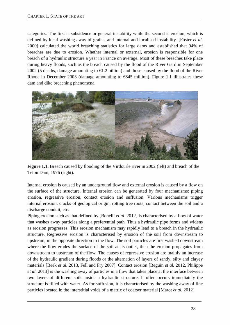
categories. The first is subsidence or general instability while the second is erosion, which is defined by local washing away of grains, and internal and localised instability. [Foster et al. 2000] calculated the world breaching statistics for large dams and established that 94% of breaches are due to erosion. Whether internal or external, erosion is responsible for one breach of a hydraulic structure a year in France on average. Most of these breaches take place during heavy floods, such as the breach caused by the flood of the River Gard in September 2002 (5 deaths, damage amounting to €1.2 billion) and those caused by the flood of the River Rhone in December 2003 (damage amounting to €845 million). Figure 1.1 illustrates these dam and dike breaching phenomena.
Figure 1.1. Breach caused by flooding of the Virdourle river in 2002 (left) and breach of the Teton Dam, 1976 (right). Internal erosion is caused by an underground flow and external erosion is caused by a flow on the surface of the structure. Internal erosion can be generated by four mechanisms: piping erosion, regressive erosion, contact erosion and suffusion. Various mechanisms trigger internal erosion: cracks of geological origin, rotting tree roots, contact between the soil and a discharge conduit, etc. Piping erosion such as that defined by [Bonelli et al. 2012] is characterised by a flow of water that washes away particles along a preferential path. Thus a hydraulic pipe forms and widens as erosion progresses. This erosion mechanism may rapidly lead to a breach in the hydraulic structure. Regressive erosion is characterised by erosion of the soil from downstream to upstream, in the opposite direction to the flow. The soil particles are first washed downstream where the flow erodes the surface of the soil at its outlet, then the erosion propagates from downstream to upstream of the flow. The causes of regressive erosion are mainly an increase of the hydraulic gradient during floods or the alternation of layers of sandy, silty and clayey materials [Beek et al. 2013, Fell and Fry 2007]. Contact erosion [Beguin et al. 2012, Philippe et al. 2013] is the washing away of particles in a flow that takes place at the interface between two layers of different soils inside a hydraulic structure. It often occurs immediately the structure is filled with water. As for suffusion, it is characterised by the washing away of fine particles located in the interstitial voids of a matrix of coarser material [Marot et al. 2012].
CHAPTER 1. STATE OF THE ART
29
1.1.1.2. Estimation of soil erodibility The objective of the decree issued on 11 December 2007 was to improve the safety of hydraulic structures in France. In particular it gives priority to revising the procedures for monitoring and studying the hazards for certain structures. So that the managers of hydraulic structures can assess their reliability, it is necessary to quantify the erosion resistance of the soils that compose them. A certain number of mechanical tests on soils have been developed to estimate their erodibility. Mention can first be made of erosion tests in flumes, used by [Gibbs 1962, Partheniades 1965] among others. The soil samples are placed in a flume on all or part of its surface. The mass eroded is either determined by weighing the samples (Hydraulic Flume Test) or by measuring the particles in the flow at the flume outlet. The Erosion Function Apparatus (EFA) developed by [Briaud 2001] also consists in passing a flow at a controlled velocity over the surface of a soil sample. The erosion rate of the soil is controlled by a piston system located under the sample. These tests aim to be representative of external erosion such as the erosion of river beds and around bridge piers. The Rotating Cylinder Test of [Moore and Mash 1962] is a cylindrical device in which a fixed cylinder of soil is placed. Water is injected between these two parts of the device and it is brought into movement. The Drill Hole Test of [Lefebvre et al. 1985] is inspired by the Rotating Cylinder Test. An initial cylindrical hole of about 6 mm in diameter is made in a soil sample in which a flow under pressure is made to circulate. This test gave rise to the Hole Erosion Test (HET) of [Wan and Fell 2004] with a controlled flow rate. The quantity of mass eroded is calculated on the basis of measurements taken upstream and downstream of the soil sample. The Hole Erosion Test is representative of internal piping erosion. Jet erosion meters have also been the subject of many studies. Their advantage is that they can be used in-situ. The Mobile Jet erodibility meter [Hénensal 1983] consists of the impact of seven mobile jets on the interface of the material. The rate of erosion is calculated from the measurement of the quantity of soil in the flow leaving the device. This device is designed to simulate the impact of rain droplets and runoff. The Jet Erosion Test (JET) developed by [Hanson and Cook 2004] is an erosion test during which a jet with a controlled flow rate impinges on the surface of a soil sample. The entire system is immerged in a tank adapted for the laboratory and the field. Erodibility is calculated by measuring the depth of the cavity formed as a function of the time the jet impinges on the material. This test is representative of external erosion by spillover downstream of the structure.
1.1.1.3. Erosion parameters The Hole Erosion Test and Jet Erosion Test are adapted to characterising the resistance of soils to erosion for embankment dams and dikes. The interpretation models of these two tests are based on an erosion law that considers erodibility as function of shear stress exerted by the soil on the soil sample. This law is governed by two parameters characteristic of soil resistance to erosion. It entails an erosion threshold from which the hydraulic power supplied is sufficient to generate erosion and an erosion coefficient. The erosion threshold is a critical
CHAPTER 1. STATE OF THE ART
30
shear stress that can range from 0 to103 Pa. The erosion coefficient also varies by several orders of magnitude, from 10-2 to 10-6 s/m. It is a coefficient of proportionality between the mass flux of the eroded soil and the shear stress exerted by the fluid on the soil (minus the critical shear stress). It can be considered as the ratio between a characteristic dimension and the surface viscosity of the eroded soil [Bonelli et al. 2012]. The erosion threshold and the erosion coefficient are used to classify the soils on a scale of erodibility. They also provide the bases of models to determine the time to breaching of structures. These parameters are a priori intrinsic to the soil and therefore should be the same whatever the test considered. However, [Regazzoni et al. 2008, Wahl et al. 2008] showed that for the same soil, the erosion parameters obtained with the JET and HET can differ by one or two orders of magnitude.
1.1.2. HET and JET erosion tests
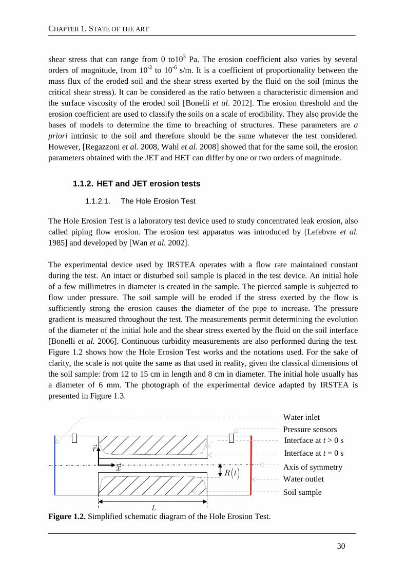
1.1.2.1. The Hole Erosion Test The Hole Erosion Test is a laboratory test device used to study concentrated leak erosion, also called piping flow erosion. The erosion test apparatus was introduced by [Lefebvre et al. 1985] and developed by [Wan et al. 2002]. The experimental device used by IRSTEA operates with a flow rate maintained constant during the test. An intact or disturbed soil sample is placed in the test device. An initial hole of a few millimetres in diameter is created in the sample. The pierced sample is subjected to flow under pressure. The soil sample will be eroded if the stress exerted by the flow is sufficiently strong the erosion causes the diameter of the pipe to increase. The pressure gradient is measured throughout the test. The measurements permit determining the evolution of the diameter of the initial hole and the shear stress exerted by the fluid on the soil interface [Bonelli et al. 2006]. Continuous turbidity measurements are also performed during the test. Figure 1.2 shows how the Hole Erosion Test works and the notations used. For the sake of clarity, the scale is not quite the same as that used in reality, given the classical dimensions of the soil sample: from 12 to 15 cm in length and 8 cm in diameter. The initial hole usually has a diameter of 6 mm. The photograph of the experimental device adapted by IRSTEA is presented in Figure 1.3.
Figure 1.2. Simplified schematic diagram of the Hole Erosion Test.
L
r
x
( )R t
Water inlet
Axis of symmetry
Soil sample
Pressure sensors
Water outlet
Interface at t = 0 s
Interface at t > 0 s
CHAPTER 1. STATE OF THE ART
31
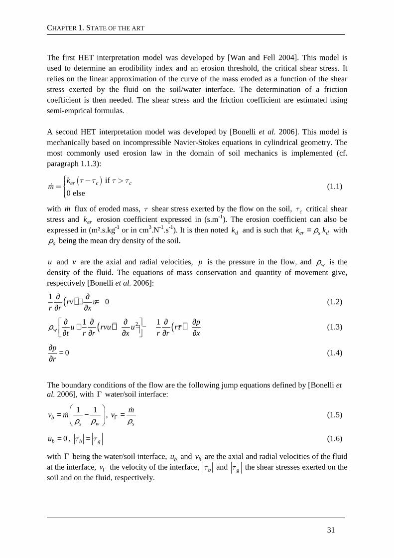
The first HET interpretation model was developed by [Wan and Fell 2004]. This model is used to determine an erodibility index and an erosion threshold, the critical shear stress. It relies on the linear approximation of the curve of the mass eroded as a function of the shear stress exerted by the fluid on the soil/water interface. The determination of a friction coefficient is then needed. The shear stress and the friction coefficient are estimated using semi-emprical formulas. A second HET interpretation model was developed by [Bonelli et al. 2006]. This model is mechanically based on incompressible Navier-Stokes equations in cylindrical geometry. The most commonly used erosion law in the domain of soil mechanics is implemented (cf. paragraph 1.1.3):
( ) if
0 elseer c ck
mɺτ τ τ τ − >=
(1.1)
with mɺ flux of eroded mass, τ shear stress exerted by the flow on the soil, τc critical shear stress and erk erosion coefficient expressed in (s.m-1). The erosion coefficient can also be expressed in (m².s.kg-1 or in cm3.N-1.s-1). It is then noted dk and is such that =er s dk kρ with
sρ being the mean dry density of the soil. u and v are the axial and radial velocities, p is the pressure in the flow, and wρ is the density of the fluid. The equations of mass conservation and quantity of movement give, respectively [Bonelli et al. 2006]:
( )10rv u
r r x
∂ ∂+ =∂ ∂
(1.2)
( ) ( )21 1w
pu rvu u r
t r r x r r x
∂ ∂ ∂ ∂ ∂ + + = − − ∂ ∂ ∂ ∂ ∂ ρ τ (1.3)
0p
r
∂ =∂
(1.4)
The boundary conditions of the flow are the following jump equations defined by [Bonelli et al. 2006], with Γ water/soil interface:
1 1 = −
b
s w
v mρ ρ
ɺ , Γ =s
mv
ρɺ
(1.5)
0bu = , τ τb g= (1.6)
with Γ being the water/soil interface, bu and bv are the axial and radial velocities of the fluid at the interface, vΓ the velocity of the interface, τb and τg the shear stresses exerted on the soil and on the fluid, respectively.
CHAPTER 1. STATE OF THE ART
32
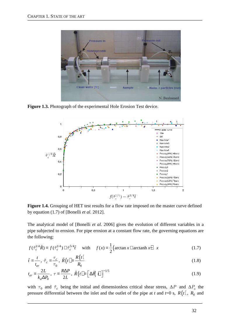
Figure 1.3. Photograph of the experimental Hole Erosion Test device.
Figure 1.4. Grouping of HET test results for a flow rate imposed on the master curve defined by equation (1.7) of [Bonelli et al. 2012]. The analytical model of [Bonelli et al. 2006] gives the evolution of different variables in a pipe subjected to erosion. For pipe erosion at a constant flow rate, the governing equations are the following:
1/4 1/4 5/4( ) ( )τ τ τc c cf R f t= +ɶ ɶɶ ɶ ɶ with ( )1( ) arctan arctanh
2f x x x x= + − (1.7)
er
tt
t=ɶ ,
0
ττ
τ
cc =ɶ , ( ) ( )
0
R tR t
R=ɶ (1.8)
0
2er
d
Lt
k P=
∆,
2τ
R P
L
∆= , ( ) ( ) 1/5R t P t
− = ∆
ɶ ɶ (1.9)
with 0τ and τcɶ being the initial and dimensionless critical shear stress, ∆P and ∆0P the
pressure differential between the inlet and the outlet of the pipe at t and t=0 s, ( )R t , 0R and
CHAPTER 1. STATE OF THE ART
33
( )R tɶ
the radius of the erodible pipe of length L at time t, initially and with a dimensionless radius; t , ert and tɶ time, the characteristic time and the dimensionless time. The validation of this simplified model was performed for different HETs, as can be seen in Figure 1.4.
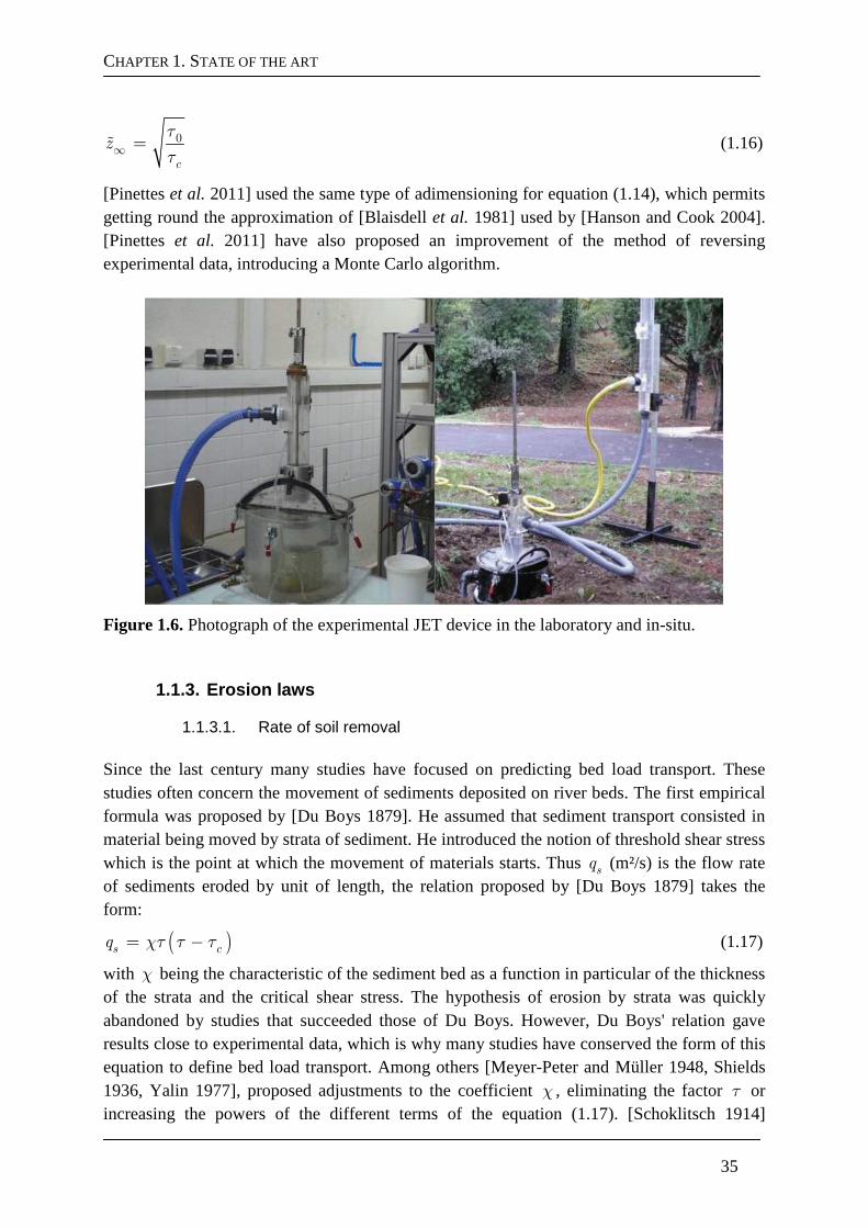
1.1.2.2. The Jet Erosion Test The Jet Erosion Test is an erosion measurement device characterised by an immersed water jet impinging on the soil surface. The test device is used to study the resistance of soils to erosion in the laboratory and in-situ. Many studies have used jets to quantify the characteristic parameters of a soil subject to erosion in the laboratory [Hanson and Robinson 1993, Hollick 1976, Mazurek et al. 2001, Moore and Mash 1962] and in-situ[Allen et al. 1997, Hanson 1991]. The experimental test device developed by [Hanson and Cook 2004] and the associated methodology initiated a large number of experimental studies to determine erodibility, including [Langendoen et al. 2000, Pinettes et al. 2011, Regazzoni et al. 2008, Robinson et al. 2000, Simon and Thomas 2002]. The soil sample can be part of the hydraulic structure in-situ, or intact or disturbed in the laboratory. It is subjected to flow under pressure. The water is set in circulation with a constant pressure drop. The flow is perpendicular to the impinged region. The soil sample will be eroded if the shear stress exerted by the flow is sufficiently strong. Measurements of scouring depth are performed throughout the test. They allow determining the characteristic parameters of the soil subjected to erosion: the erosion coefficient and the critical shear stress. Figure 1.5 shows how the Jet Erosion Test works and the notations used. Figure 1.6 presents two photographs of the experimental test device in the laboratory and in-situ. This apparatus is that used at present by geophyConsult [Pinettes et al. 2011], and it was also used for the study [Regazzoni et al. 2008]. The interpretation model of the Jet Erosion Test was developed by [Hanson and Cook 2004]. It is based on the analytical approach of [Stein and Nett 1997] developed in the case of plane jets. The governing equations of the model of [Hanson and Cook 2004], excluding the erosion law (1.1) are the following:
0 2U g H= ∆ (1.10)
( ) 0
lU z U
z= (1.11)
06.2l d= × (1.12)
( )2
f wC U zτ ρ= (1.13)
with g being gravity, 0U the velocity of the jet at the nozzle, H∆ the hydraulic head applied, l the potential core length, z the distance separating the height of the jet outlet and
CHAPTER 1. STATE OF THE ART
34
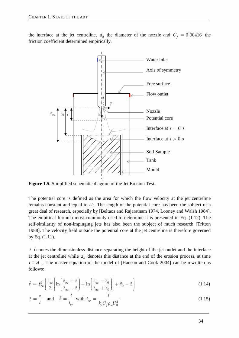
the interface at the jet centreline, 0d the diameter of the nozzle and = 0 00416fC . the friction coefficient determined empirically.
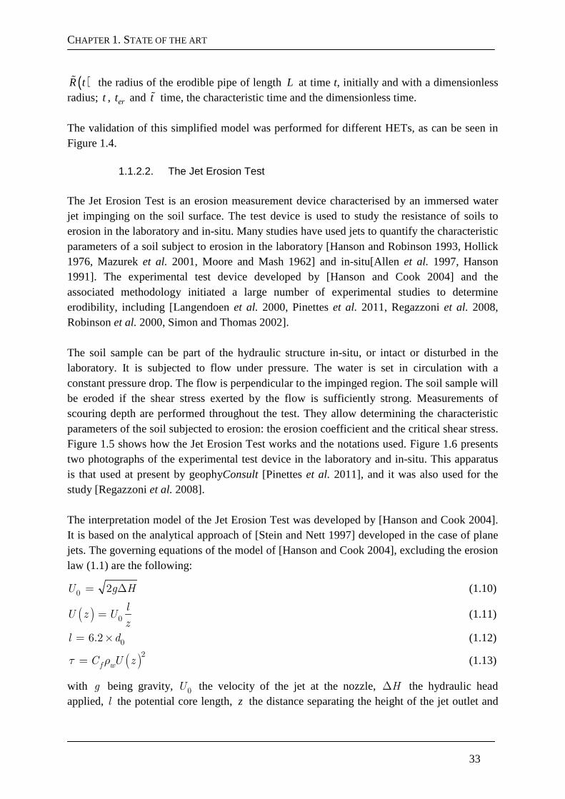
Figure 1.5. Simplified schematic diagram of the Jet Erosion Test.
The potential core is defined as the area for which the flow velocity at the jet centreline remains constant and equal to U0. The length of the potential core has been the subject of a great deal of research, especially by [Beltaos and Rajaratnam 1974, Looney and Walsh 1984]. The empirical formula most commonly used to determine it is presented in Eq. (1.12). The self-similarity of non-impinging jets has also been the subject of much research [Tritton 1988]. The velocity field outside the potential core at the jet centreline is therefore governed by Eq. (1.11). zɶ denotes the dimensionless distance separating the height of the jet outlet and the interface at the jet centreline while z∞ denotes this distance at the end of the erosion process, at time
= +∞t . The master equation of the model of [Hanson and Cook 2004] can be rewritten as follows:
2 00
0
ln ln2
z z z z zt z z z
z z z z∞ ∞ ∞
∞∞ ∞
+ − = + + − − +
ɶ ɶ ɶ ɶ ɶɶ ɶ ɶ ɶ
ɶ ɶ ɶ ɶ (1.14)
zz
l=ɶ and
er
ttt
=ɶ with 20
er
d f w
lt
k C Uρ= (1.15)
Water inlet
Axis of symmetry
Free surface
Flow outlet
Nozzle
Potential core
Interface at 0t = s z Interface at 0 st >
Soil Sample
Mould
Tank
z∞ 0
z l z
r
0 d
CHAPTER 1. STATE OF THE ART
35
0
c
zτ
τ∞ =ɶ (1.16)
[Pinettes et al. 2011] used the same type of adimensioning for equation (1.14), which permits getting round the approximation of [Blaisdell et al. 1981] used by [Hanson and Cook 2004]. [Pinettes et al. 2011] have also proposed an improvement of the method of reversing experimental data, introducing a Monte Carlo algorithm.
Figure 1.6. Photograph of the experimental JET device in the laboratory and in-situ.
1.1.3. Erosion laws
1.1.3.1. Rate of soil removal Since the last century many studies have focused on predicting bed load transport. These studies often concern the movement of sediments deposited on river beds. The first empirical formula was proposed by [Du Boys 1879]. He assumed that sediment transport consisted in material being moved by strata of sediment. He introduced the notion of threshold shear stress which is the point at which the movement of materials starts. Thus sq (m²/s) is the flow rate of sediments eroded by unit of length, the relation proposed by [Du Boys 1879] takes the form:
( )s cq χτ τ τ= − (1.17)
with χ being the characteristic of the sediment bed as a function in particular of the thickness of the strata and the critical shear stress. The hypothesis of erosion by strata was quickly abandoned by studies that succeeded those of Du Boys. However, Du Boys' relation gave results close to experimental data, which is why many studies have conserved the form of this equation to define bed load transport. Among others [Meyer-Peter and Müller 1948, Shields 1936, Yalin 1977], proposed adjustments to the coefficient χ , eliminating the factor τ or increasing the powers of the different terms of the equation (1.17). [Schoklitsch 1914]
CHAPTER 1. STATE OF THE ART
36
proposed considering sq as a linear function of the flow rate rather than considering the influence of the shear stress. Other studies, such as that of [Barekyan 1962] established a relation between the erosion rate, velocity and the flow rate. In the formulation developed by [Einstein 1950], the critical shear stress is no longer taken into account and the erosion rate depends on fluctuations of velocity. The models developed by [Einstein 1950, Meyer-Peter and Müller 1948, Yalin 1977] gave very similar results. Historically, using the correlation of [Meyer-Peter and Müller 1948] became very widespread in Europe whereas that of [Einstein 1950] was commonly used in the United States. Other studies such as those of [Bagnold 1956, Engelund and Hansen 1967] gave total solid transport as volume of grains at saturation. The formulation proposed therefore dealt with bed load and suspension. All these different bed load transport models were formulated empirically in the framework of the erosion of granular soils. Likewise for more recent models stemming from them such as those of [Rickenmann and Recking 2011, Wilcock and Crowe 2003]. That is why these models cannot be adapted to our configurations. Very finalised models relying on biphasic media have been developed. They involve laminar flows on granular media but these models do not, a priori, include erosion laws. [Papamichos and Vardoulakis 2005] developed an erosion model using finite elements. It permits predicting the production of sand by erosion in the oil exploration sector. A fluidised solid phase was introduced. The three phase system is resolved using mass conservation equations, Darcy's law, and by introducing an erosion law based on the diffusion of porosity. As for [Ouriemi et al. 2009, Chauchat and Médale 2010], they focused on the bed load transport of a sediment bed. The mobile medium is considered as a granular medium in which the particles are in contact. The modelling is biphasic, the forces at the interface are calculated by Darcy's law and by the law governing buoyancy [Jackson 2000]. Adapted to laminar flows on granular soils, these models discussed in paragraph 1.2 are ill-suited for modelling a fine cohesive soil by a turbulent flow. Regarding cohesive soils impinged by a turbulent flow, [Ariathurai and Arulanandan 1978] were the first to introduce the erosion law now used most frequently, Eq. (1.1). They based their work on the experimental results obtained by [Partheniades 1965]. These experimental results tended to point to the existence of a linear relation between the erosion rate and the residual shear stress. This is defined as the subtraction of the critical shear stress from the shear stress. It is noteworthy that [Partheniades 1965] opted instead for the development of an erosion law based on the probability of erosion by strata of cohesive sediments. This law is an exponential relation of the cohesion force of particles and shear stress. The concentration of sediments in suspension in the fluid phase is determined experimentally. It is then converted into a flux of eroded mass using an empirical formula that estimates the erosion in a channel about 18 m long. However, depending on the velocity of the flow considered, the erosion process does not necessarily end only with the detachment of particles. Phenomena related to particle transport such as re-deposition may occur. However, the linearity of the relation of erosion rate as a function of critical shear stress has been validated in very different flow configurations. A certain number of experimental studies have since demonstrated this
CHAPTER 1. STATE OF THE ART
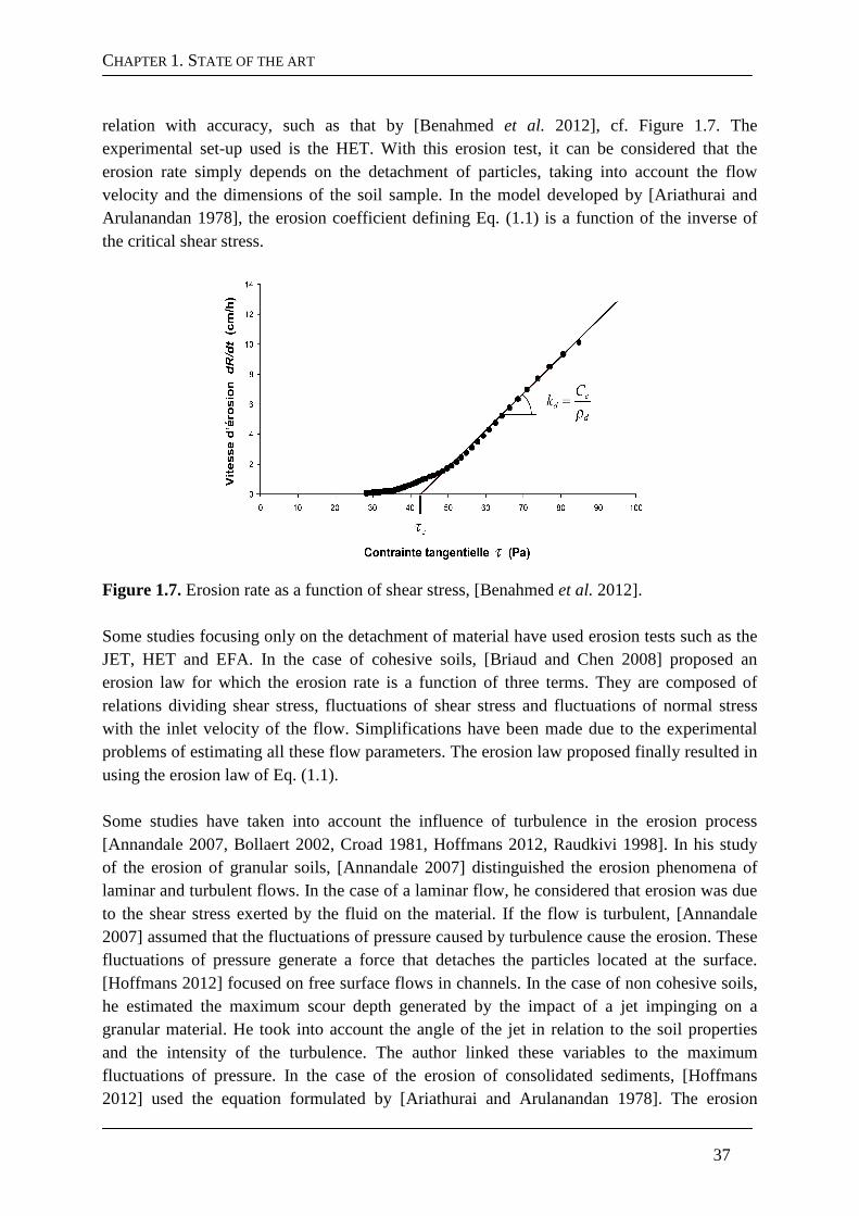
37
relation with accuracy, such as that by [Benahmed et al. 2012], cf. Figure 1.7. The experimental set-up used is the HET. With this erosion test, it can be considered that the erosion rate simply depends on the detachment of particles, taking into account the flow velocity and the dimensions of the soil sample. In the model developed by [Ariathurai and Arulanandan 1978], the erosion coefficient defining Eq. (1.1) is a function of the inverse of the critical shear stress.
Figure 1.7. Erosion rate as a function of shear stress, [Benahmed et al. 2012]. Some studies focusing only on the detachment of material have used erosion tests such as the JET, HET and EFA. In the case of cohesive soils, [Briaud and Chen 2008] proposed an erosion law for which the erosion rate is a function of three terms. They are composed of relations dividing shear stress, fluctuations of shear stress and fluctuations of normal stress with the inlet velocity of the flow. Simplifications have been made due to the experimental problems of estimating all these flow parameters. The erosion law proposed finally resulted in using the erosion law of Eq. (1.1). Some studies have taken into account the influence of turbulence in the erosion process [Annandale 2007, Bollaert 2002, Croad 1981, Hoffmans 2012, Raudkivi 1998]. In his study of the erosion of granular soils, [Annandale 2007] distinguished the erosion phenomena of laminar and turbulent flows. In the case of a laminar flow, he considered that erosion was due to the shear stress exerted by the fluid on the material. If the flow is turbulent, [Annandale 2007] assumed that the fluctuations of pressure caused by turbulence cause the erosion. These fluctuations of pressure generate a force that detaches the particles located at the surface. [Hoffmans 2012] focused on free surface flows in channels. In the case of non cohesive soils, he estimated the maximum scour depth generated by the impact of a jet impinging on a granular material. He took into account the angle of the jet in relation to the soil properties and the intensity of the turbulence. The author linked these variables to the maximum fluctuations of pressure. In the case of the erosion of consolidated sediments, [Hoffmans 2012] used the equation formulated by [Ariathurai and Arulanandan 1978]. The erosion
CHAPTER 1. STATE OF THE ART
38
coefficient here depends on the characteristics of the sediments, a consolidation parameter and the inverse of the critical shear stress. The critical shear stress, defined by the Shields parameter (cf. paragraph 1.1.3.2), is then linked to the maximum of the pressure fluctuations:
00 0
*
m m
k ur
U Uα= = with τ ρ 2*
wu= (1.18)
( )τα τ ρ2
012 6m w mp . rU= = (1.19)
( )c c s w gdτ θ ρ ρ= − , ( )
( )
2
00 7 mw
s w c
rUd .
gρρ ρ θ
=−
(1.20)
with mp being the maximum pressure fluctuations, 0r the intensity of the turbulence averaged between the surface of the soil and the free surface, mU and 0k the velocity of the flow and the turbulent kinetic energy averaged in the same way, *u the friction velocity at the soil/water interface, 0α and τα constants determined empirically of values 1.2 and 18 respectively for uniform flows, and cθ the critical Shields number and d the grain diameter. This empirical model adapted to free surface flows is not directly applicable to our configurations. Nonetheless, this way of taking turbulence into account in an erosion model remains interesting. Furthermore, [Kobus et al. 1979] showed experimentally that pulsating jets lead to deeper erosion figures than stabilised jets. [Cleaver and Yates 1973, Croad 1981, Nearing 1991, Sharif and Atkinson 2012] focused on the detachment of particles under the effect of a shallow free surface flow, similar to that of waves breaking on a beach. These studies highlight the influence of turbulent bursts causing the detachment of grains. [Haehnel and Dade 2008] performed an experimental study of a turbulent air jet impinging on a granular medium. They showed that erosion is governed by the shear stress defined by (cf. paragraph 2.3.1 for the general definition of the shear stress)
wallw v' w'τ ρ
→= (1.21)
0 2v' w' . k= , ( )2 2 21
2k u' v' w'= + + (1.22)
with v' and w' being fluctuations of velocity calculated close to the surface of grains and k the turbulent kinetic energy. The problem of determining the distance to the wall, which is the point at which we place ourselves to calculate the fluctuations of velocities, is a major issue that remains to be solved. The erosion of soils by impinging jets at the surface of the soil has been the subject of many experimental studies [Dunn 1959, Hanson et al. 1990, Hollick 1976, Mazurek and Hossain 2007, Moore and Masch 1962, O'Donoghue et al. 2001, Rajaratnam 1982, Rouse 1939, Stein and Nett 1997]. They permit estimating the dimensions of the cavity formed as a function of time or at the end of the erosion process. In a configuration similar to that of the JET, [Mazurek and Hossain 2007] focused on the erosion of soils, cohesive or not, caused by a
CHAPTER 1. STATE OF THE ART
39
turbulent jet. [Rajaratnam 1982] and [Mazurek et al. 2001] found that the dimensions of the cavity formed for cohesive and non cohesive soils evolve proportionally to a logarithm of time. This validates the relations of [Moore and Mash 1962, Rouse 1939]. The experimental observations of [Rajaratnam 1982] performed at the end of the erosion process showed that the dimensions of the erosion cavities depend on the velocity at the jet nozzle, the size of the grains and the densities of the fluid and the soil. [O'Donoghue et al. 2001] proposed the same type of valid empirical relation for wide ranges of nozzle diameters, grain sizes and distances between the jet nozzle and soil surface. [Mazurek et al. 2001] showed that for a cohesive soil, these dimensions depend on the velocities of the jet at the nozzle outlet, the density of the fluid and the ratio of the nozzle diameter over the scour depth and over the scour depth at the end of the erosion process. Analytical approaches based on energetic analyses have also been developed. These methods permit determining the shape of the erosion figure as a function of several variables, but they do not give any law for the evolution of erodibility. The erosion of soils by jets tangent to the surface of the soil, on a free surface, has also been the subject of several studies in the case of granular media [Dey and Westrich 2003, Hogg et al. 1997, Hopfinger et al. 2004]. [Hopfinger et al. 2004] linked sediment erosion to the eddies defined by [Görtler 1941]. These eddies are induced in laminar or turbulent flow next to a concave wall. In a configuration similar to that of the HET and for cohesive soils, [Indraratna et al. 2009] proposed to estimate the variations of the pipe diameters using the geotechnical properties of the soil and the energy necessary to ensure detachment. A clear distinction is made between the detachment and the transport of particles, although erosion is defined as the result of both of these phenomena. [Regazzoni and Marot 2011] proposed an energetic analysis of the JET and HET in which the transport of eroded particles is omitted. No erosion law is defined, but a new index of resistance of the soil to erosion is introduced. This new index is used to establish a new classification of soils. Thus, despite the erosion laws on bed load transport or on granular media that cannot be adapted to our problem, a large number of empirical laws have been developed in very specific configurations. Many studies do not propose an erosion law but make predictions on the shape of erosion figures. Apart from the classical erosion law which appears to give good results, no other erosion law is directly applicable to our configurations. However, it is interesting to observe that some studies consider that erosion is governed by turbulence variables.
1.1.3.2. Determination of critical shear stress Regarding the detachment of non cohesive particles, [Shields 1936] introduced a stability criterion beyond which the particle considered will be set in motion by the flow. The configuration of Shields' study initially involved the erosion of river beds. The Shields number is defined as the ratio of the forces permitting movement over inertial force. It is the
CHAPTER 1. STATE OF THE ART
40
ratio of shear stress exerted at the surface of the grain over the buoyancy exerted on the grain. The setting in motion of the grains is effective when the Shields number exceeds a critical value. This value is linked experimentally to the particle Reynolds number. Thus cθ is the critical Shields number and fγ a function that can be described graphically:
( )( )c
c ps w
f Regd
γ
τθ
ρ ρ= =
− (1.23)
*.p
w
u dRe
ν= (1.24)
with Rep being the particle Reynolds number and wν the kinematic viscosity of the fluid. It is difficult in practice to determine the critical Shields parameter in any given flow configuration. Indeed, the critical Shields parameter and the particle Reynolds number depend on the shear stress, difficult to determine in practice. In the case of free surface flows, the friction velocity is known and defined as a function of the hydraulic radius of the channel and its slope. [Buffington and Montgomery 1997] carried out an exhaustive synthesis of all the studies aimed at improving or revising the Shields curve since its publication. Considerable dispersion of experimental data can be observed. [Buffington and Montgomery 1997] explained that these differences are due to very different experimental protocols. Detection methods, flow regimes and grain properties vary considerably depending on the study concerned. This has also been observed for the methods used to determine the critical shear stress exerted by the fluid on the grains. [Yalin 1977] proposed defining the Shields number as a function of the dimensionless diameter of the grain dɶ :
( )βθc f d= ɶ with ( )ρ ρ
ρ ν
1/3
2
s w
w w
gd
d
− =
ɶ
(1.25)
where fβ is a function described graphically. An adjustment of the Shields curve was proposed by [Yalin and Ferreira Da Silva 2001]. As for [Cao 2006], who proposed an explicit formula to estimate the critical Shields value. The expression obtained makes it easier to determine the critical Shields number, in agreement with the experimental and bibliographical data. In the case of granular soils, [Hoffmans 2012] and [Annandale 2007] calculated the Shields parameter from the pressure fluctuations due to turbulence. These fluctuations are estimated using the empirical models of [Hinze 1975] and [Emmerling 1973], cf. paragraph 1.1.3.1. In the case of cohesive soils or consolidated sediments, some studies have proposed adaptations of the Shields parameter. They introduce a factor relative to adhesion force. [Dade et al. 1992] considered a ratio between adhesion forces and the deadweight of the particles. [Gargani 2004, Ternat et al. 2008] proposed taking into account a parameter relative to Van der Waals forces. [Claudin and Andreotti 2006] took surface tension into account. The data required for the application of these models are difficult to obtain for real cohesive soils: the
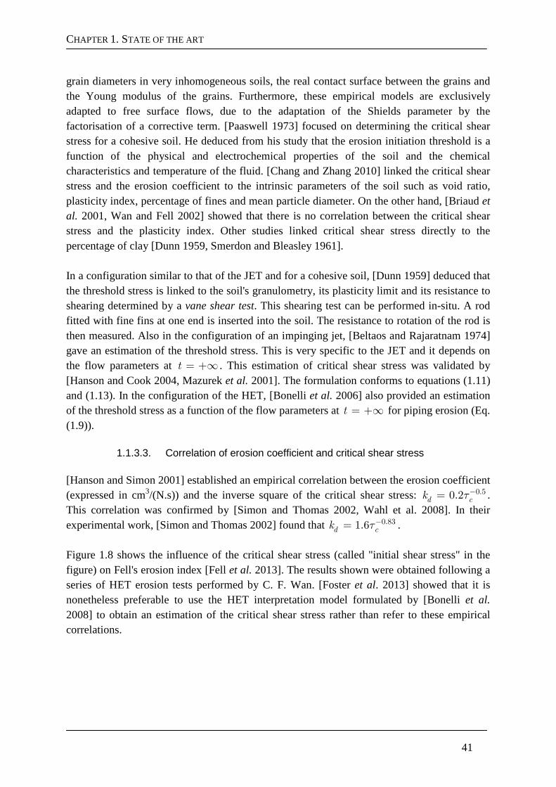
CHAPTER 1. STATE OF THE ART
41
grain diameters in very inhomogeneous soils, the real contact surface between the grains and the Young modulus of the grains. Furthermore, these empirical models are exclusively adapted to free surface flows, due to the adaptation of the Shields parameter by the factorisation of a corrective term. [Paaswell 1973] focused on determining the critical shear stress for a cohesive soil. He deduced from his study that the erosion initiation threshold is a function of the physical and electrochemical properties of the soil and the chemical characteristics and temperature of the fluid. [Chang and Zhang 2010] linked the critical shear stress and the erosion coefficient to the intrinsic parameters of the soil such as void ratio, plasticity index, percentage of fines and mean particle diameter. On the other hand, [Briaud et al. 2001, Wan and Fell 2002] showed that there is no correlation between the critical shear stress and the plasticity index. Other studies linked critical shear stress directly to the percentage of clay [Dunn 1959, Smerdon and Bleasley 1961]. In a configuration similar to that of the JET and for a cohesive soil, [Dunn 1959] deduced that the threshold stress is linked to the soil's granulometry, its plasticity limit and its resistance to shearing determined by a vane shear test. This shearing test can be performed in-situ. A rod fitted with fine fins at one end is inserted into the soil. The resistance to rotation of the rod is then measured. Also in the configuration of an impinging jet, [Beltaos and Rajaratnam 1974] gave an estimation of the threshold stress. This is very specific to the JET and it depends on the flow parameters at t = +∞ . This estimation of critical shear stress was validated by [Hanson and Cook 2004, Mazurek et al. 2001]. The formulation conforms to equations (1.11) and (1.13). In the configuration of the HET, [Bonelli et al. 2006] also provided an estimation of the threshold stress as a function of the flow parameters at t = +∞ for piping erosion (Eq. (1.9)).
1.1.3.3. Correlation of erosion coefficient and critical shear stress [Hanson and Simon 2001] established an empirical correlation between the erosion coefficient (expressed in cm3/(N.s)) and the inverse square of the critical shear stress: 0.50.2d ck −= τ . This correlation was confirmed by [Simon and Thomas 2002, Wahl et al. 2008]. In their experimental work, [Simon and Thomas 2002] found that 0.831.6d ck −= τ . Figure 1.8 shows the influence of the critical shear stress (called "initial shear stress" in the figure) on Fell's erosion index [Fell et al. 2013]. The results shown were obtained following a series of HET erosion tests performed by C. F. Wan. [Foster et al. 2013] showed that it is nonetheless preferable to use the HET interpretation model formulated by [Bonelli et al. 2008] to obtain an estimation of the critical shear stress rather than refer to these empirical correlations.
CHAPTER 1. STATE OF THE ART
42
Figure 1.8. Influence of the critical shear stress on the erosion coefficient [Fell et al. 2013].
1.2. Numerical modelling of erosion
1.2.1. Context
1.2.1.1. Erosion of granular soils and cohesive soils The numerical modelling of erosion has been the subject of many studies over the past twenty years. Two erosion modelling methods have been validated for laminar flows on granular beds. The first empirical formula was proposed by [Vardoulakis et al. 1996]. It introduced a third fluidised solid phase between the fluid and solid phases. This phase is resolved by Darcy-Brinkman equations. The erosion of the solid phase is described by a source term. This term induces exchanges of mass between the soil and fluid phases in the mass conservation equations. The second empirical formula was proposed by [Ouriemi et al. 2009]. The solid and fluid phases interact through quantity of movement exchanges. The equations of biphasic media developed by [Jackson 2000] form the basis of the transport equations used in this model. These two methods and their adaptability to our configurations are discussed in paragraph 1.2.2. In the framework of modelling the erosion of a fine cohesive soil by a turbulent flow, the solid/fluid interface can be considered singular, and not as a third fluidised solid phase. Each phase is biphasic: a compact assembly of particles containing water and water containing particles in dispersed phase. The difficulty therefore lies in representing the mobile interface and precisely calculating the mechanical quantities on the interface. Two approaches can be
CHAPTER 1. STATE OF THE ART
43
distinguished in the framework of the numerical simulation of flows in the presence of interfaces: capturing and monitoring the interface. The first, called the Eulerian approach, consists in defining the media (water-soil) in a given domain (fixed mesh) and determining its evolution. The second, a mixed Eulerian-Lagrangian approach, consists in displacing the frontier through time and adapting the mesh.
1.2.1.2. Different approaches to model interfaces Modelling the interface separating a fluid and a solid is highly complex, since each medium is usually described through very different approaches. Fluid is more naturally described using Eulerian models and the soil by Lagrangian models. The mixed Eulerian-Lagrangian approaches introduced by [Donea et al. 1982] achieve a good compromise between the two descriptions. The two media are defined within a mobile mesh while the Eulerian and Lagrangian resolutions of the solid and fluid behaviours, respectively, are independent. The Eulerian equations of the fluid are first calculated independently of the Lagrangian model of the solid. The equations governing the behaviour of the solid are resolved on the basis of the results found for the fluid. The meshing of the fluid zone is deformed in correspondence with the results obtained for the solid. The equations of the fluid are calculated within the updated mesh, and so forth. The mixed Eulerian-Lagrangian methods ensure great simplicity in the formulation of the equations governing the behaviours of the fluid and the solid and they lead to considerable gains in calculation time. Furthermore, the advantage of the method is that it provides a fine description of the flow variables at the interface. Its disadvantage is that it is limited by the distortion of the mesh, making it necessary to consider remeshing methods. Remeshing can introduce major problems, especially in 3D geometry, and often leads to a huge increase in calculation time. Completely Eulerian methods with immersed boundaries have also been developed [Angot 2005, Peskin 1977]. The equations of the solid are written so that they resemble the fluid equations as much as possible. The main characteristic of these methods is that there are no fixed boundaries between domains, which often introduces complex meshing. The flow presenting an immersed obstacle can, for example, be calculated with a fixed Cartesian mesh independent of changes in the shape of the object. A VOF (Volume of Fluid) [DeBar 1974] or Level-Set [Osher and Sethian 1981] method can be used to localise the different domains and describe their evolution. The advantage of this method compared to mixed Euler-Lagrange models is that it requires considerably less remeshing. Although the meshing of the zones close to the interface must be refined, the extent and frequency of the remeshing required for this method are not so great. The major disadvantage of this method, however, is that it is difficult to obtain a fine resolution of the flow variables at the interface. Interpolations are required to ensure the representativeness of the position of the portion of the interface within the mesh. [Lachouette et al. 2008] developed a numerical erosion model based on this method. It permits resolving a viscous incompressible laminar flow with erosion in 2 and 3-D geometry. The interface is represented by the fictitious domains method and its evolution is described by the Level-Set method within a fixed Cartesian grid (cf. paragraph 1.2.3). The

CHAPTER 1. STATE OF THE ART
44
method is validated in the case of piping erosion in laminar regime. The results of numerical modelling of the HET for a laminar flow agree well with those obtained with the analytical model of [Bonelli et al. 2006].
1.2.2. Biphasic and triphasic models
1.2.2.1. The approach of Papamichos and Vardoulakis (2005) The erosion model of [Papamichos and Vardoulakis 2005] was developed in the framework of sand production in the oil exploration industry. They modelled the erosion of a granular soil by a laminar flow. The method developed relies on modelling the eroded medium as a triphasic medium. A set of mass conservation equations is established for each of the phases: the equation (1.26) for the solid phase, (1.27) for the fluidised solid phase and (1.28) for the fluid phase. Indexes 1, 2 and 3 correspond to the solid, fluid and fluidised solid phases respectively.
( )1
s
j
t
φ
ρ
∂= −
∂ (1.26)
( ) ( )31div i
cq
t
φ∂ −=
∂ with ( ) ( )3 2
i iq c vφ= (1.27)
div 0iq = with ( )2i i i
w
Kq v pφ
µ= = − (1.28)
with φ being the porosity of the solid elements in the fluid phase defined as the ratio of the sum of the volumes of phases (1) and (3) over the total volume of the three phases. The production term ( )1j corresponds to the rate of detachment of soil by erosion. The concentration c of solid elements in the fluid phase is defined as the ratio of the volume of phase (3) over the total volume of the three phases. The velocity of filtration iq is defined by Darcy's law with K as the intrinsic permeability, wµ the dynamic viscosity of the fluid and
ip the pressure at pore scale. This set of equations has four independent unknowns: φ , c , ( )1j and ip . An additional equation is required to resolve this system of equations, which is why a porosity diffusion behaviour law is introduced. The solid particles are driven out of regions of increasing porosity. This diffusion model can be considered as a piping erosion law in which the flow lines of the eroded particles are colinear with the porosity gradient. By assuming that the concentration in particles is low, the equation (1.26) becomes the following porosity diffusion equation, with λ being the diffusion coefficient:
iit
φλφ
∂=
∂ (1.29)
The erosion of the solid matrix is thus described and then coupled with porosity-elasticity equations. These equations allow describing the porosity-mechanical behaviour of the system.
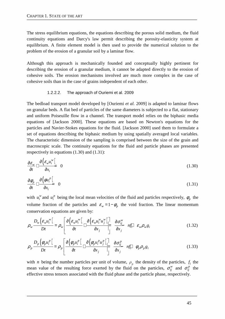
CHAPTER 1. STATE OF THE ART
45
The stress equilibrium equations, the equations describing the porous solid medium, the fluid continuity equations and Darcy's law permit describing the porosity-elasticity system at equilibrium. A finite element model is then used to provide the numerical solution to the problem of the erosion of a granular soil by a laminar flow. Although this approach is mechanically founded and conceptually highly pertinent for describing the erosion of a granular medium, it cannot be adapted directly to the erosion of cohesive soils. The erosion mechanisms involved are much more complex in the case of cohesive soils than in the case of grains independent of each other.
1.2.2.2. The approach of Ouriemi et al. 2009 The bedload transport model developed by [Ouriemi et al. 2009] is adapted to laminar flows on granular beds. A flat bed of particles of the same diameters is subjected to a flat, stationary and uniform Poiseuille flow in a channel. The transport model relies on the biphasic media equations of [Jackson 2000]. These equations are based on Newton's equations for the particles and Navier-Stokes equations for the fluid. [Jackson 2000] used them to formulate a set of equations describing the biphasic medium by using spatially averaged local variables. The characteristic dimension of the sampling is comprised between the size of the grain and macroscopic scale. The continuity equations for the fluid and particle phases are presented respectively in equations (1.30) and (1.31):
( )0
ww iw
i
u
t x
εε ∂∂+ =
∂ ∂ (1.30)
( )0
pip
i
u
t x
φφ ∂∂+ =
∂ ∂ (1.31)
with wiu and p
iu being the local mean velocities of the fluid and particles respectively, pφ the
volume fraction of the particles and 1w pε φ= − the void fraction. The linear momentum
conservation equations are given by:
( ) ( ) ( )w w w w ww w i w i w i j ij
w w i w w ij j
D u u u unf g
Dt t x x
ε ε ε σρ ρ ε ρ
∂ ∂ ∂ = + = − + ∂ ∂ ∂
(1.32)
( ) ( ) ( )p p p p pp p i p i p i j ij
p p i p p ij j
D u u u unf g
Dt t x x
φ φ φ σρ ρ φ ρ
∂ ∂ ∂ = + = − + ∂ ∂ ∂
(1.33)
with n being the number particles per unit of volume, ρp the density of the particles, if the mean value of the resulting force exerted by the fluid on the particles, w
ijσ and pijσ the
effective stress tensors associated with the fluid phase and the particle phase, respectively.
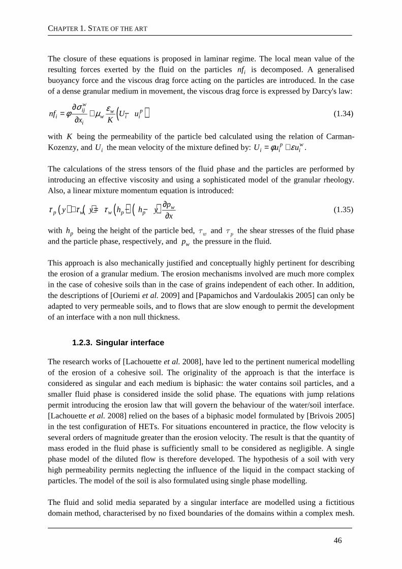
CHAPTER 1. STATE OF THE ART
46
The closure of these equations is proposed in laminar regime. The local mean value of the resulting forces exerted by the fluid on the particles inf is decomposed. A generalised buoyancy force and the viscous drag force acting on the particles are introduced. In the case of a dense granular medium in movement, the viscous drag force is expressed by Darcy's law:
( )wij pw
i w i ii
nf U ux K
σ εφ µ∂
= + −∂
(1.34)
with K being the permeability of the particle bed calculated using the relation of Carman-Kozenzy, and iU the mean velocity of the mixture defined by: p w
i i iU u uφ ε= + . The calculations of the stress tensors of the fluid phase and the particles are performed by introducing an effective viscosity and using a sophisticated model of the granular rheology. Also, a linear mixture momentum equation is introduced:
( ) ( ) ( ) ( ) wp w w p p
py y h h y
xτ τ τ ∂+ = − −
∂ (1.35)
with ph being the height of the particle bed, wτ and τp the shear stresses of the fluid phase and the particle phase, respectively, and wp the pressure in the fluid. This approach is also mechanically justified and conceptually highly pertinent for describing the erosion of a granular medium. The erosion mechanisms involved are much more complex in the case of cohesive soils than in the case of grains independent of each other. In addition, the descriptions of [Ouriemi et al. 2009] and [Papamichos and Vardoulakis 2005] can only be adapted to very permeable soils, and to flows that are slow enough to permit the development of an interface with a non null thickness.
1.2.3. Singular interface
The research works of [Lachouette et al. 2008], have led to the pertinent numerical modelling of the erosion of a cohesive soil. The originality of the approach is that the interface is considered as singular and each medium is biphasic: the water contains soil particles, and a smaller fluid phase is considered inside the solid phase. The equations with jump relations permit introducing the erosion law that will govern the behaviour of the water/soil interface. [Lachouette et al. 2008] relied on the bases of a biphasic model formulated by [Brivois 2005] in the test configuration of HETs. For situations encountered in practice, the flow velocity is several orders of magnitude greater than the erosion velocity. The result is that the quantity of mass eroded in the fluid phase is sufficiently small to be considered as negligible. A single phase model of the diluted flow is therefore developed. The hypothesis of a soil with very high permeability permits neglecting the influence of the liquid in the compact stacking of particles. The model of the soil is also formulated using single phase modelling. The fluid and solid media separated by a singular interface are modelled using a fictitious domain method, characterised by no fixed boundaries of the domains within a complex mesh.
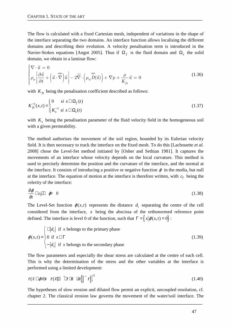
CHAPTER 1. STATE OF THE ART
47
The flow is calculated with a fixed Cartesian mesh, independent of variations in the shape of the interface separating the two domains. An interface function allows localising the different domains and describing their evolution. A velocity penalisation term is introduced in the Navier-Stokes equations [Angot 2005]. Thus if fΩ is the fluid domain and sΩ the solid domain, we obtain in a laminar flow:
( ) ( ) µρ µ
0
2 ( ) 0w wfs
u
uu u D u p u
t K
∇ ⋅ = ∂ + ⋅ ∇ − ∇ ⋅ + ∇ + = ∂
(1.36)
with fsK being the penalisation coefficient described as follows:
11
0 ( )( , )
( )
ffs
s s
si x tK x t
K si x t
−−
∈Ω= ∈Ω
(1.37)
with sK being the penalisation parameter of the fluid velocity field in the homogeneous soil with a given permeability. The method authorises the movement of the soil region, bounded by its Eulerian velocity field. It is then necessary to track the interface on the fixed mesh. To do this [Lachouette et al. 2008] chose the Level-Set method initiated by [Osher and Sethian 1981]. It captures the movements of an interface whose velocity depends on the local curvature. This method is used to precisely determine the position and the curvature of the interface, and the normal at the interface. It consists of introducing a positive or negative function ϕ in the media, but null at the interface. The equation of motion at the interface is therefore written, with cΓ being the celerity of the interface:
0ct
ϕ ϕΓ∂ + ⋅∇ =∂
(1.38)
The Level-Set function ( , )x tϕ represents the distance id separating the centre of the cell
considered from the interface, x being the abscissa of the orthonormed reference point
defined. The interface is level 0 of the function, such that ( , ) 0x x tϕΓ = = :
if belongs to the primary phase
( , ) 0 if
if belongs to the secondary phase
i
i
d x
x t x
d x
ϕ+
= ∈Γ−
(1.39)
The flow parameters and especially the shear stress are calculated at the centre of each cell. This is why the determination of the stress and the other variables at the interface is performed using a limited development:
( )2( ) ( )x n x nτ ϕ τ τ ο τ+ = + ∇ ⋅ + ∇
(1.40)
The hypotheses of slow erosion and diluted flow permit an explicit, uncoupled resolution, cf. chapter 2. The classical erosion law governs the movement of the water/soil interface. The
CHAPTER 1. STATE OF THE ART
48
results given by the modelling method in the case of a plane laminar Poiseuille flow agree well with the known theoretical solution. The model of [Lachouette et al. 2008] is applied to a configuration similar to that of the HET but for a laminar flow. The numerical results are compared with the analytical model of [Bonelli et al. 2006] and good agreement is obtained. Nonetheless, in the framework of the numerical modelling of the erosion of a cohesive soil by a turbulent flow, it is necessary to thoroughly determine the quantities at the water/soil interface. That is why it is preferable to opt for a mixed Eulerian-Lagrangian model.
1.3. Conclusions on the state of the art
Firstly, the general context of the risks related to hydraulic structures was described, and mention was made of the challenges of performing a reliable determination of the erodibility of soils. We then studied the different systems used to determine the behaviour of soils subjected to erosion. The characteristic parameters of soils, i.e. critical shear stress and erosion coefficient were defined. A full description of the JET and HET tests and the interpretation models were then provided. This was followed by a presentation of the state of the art of the erosion law. A large number of studies propose models for determining the erosion rate and for determining the critical shear stress in the case of granular media. However, these models are not adapted to cohesive soils. Other models can be used on cohesive soils but they are often very empirical and adapted to specific configurations or use a set of soil characteristics that are very difficult to determine for real cohesive soils. The erosion law most commonly used is the so-called classical erosion law of [Ariathurai and Arulanandan 1978]. The linearity of the relation between the shear stress and the erosion rate has been the subject of several validations. However, it is interesting to observe that the variables linked to turbulence are sometimes considered as variables governing erosion. Secondly, the state of the art regarding the numerical modelling of erosion was provided. The approaches of [Vardoulakis et al. 1996] and [Ouriemi et al. 2009] were described for the erosion of granular media. They were mechanically based and have been validated. Nonetheless, these models are not adapted to modelling the erosion of cohesive soils. The approach of [Lachouette et al. 2008] is adapted to the erosion of cohesive soils and includes the movement of a singular water/soil interface. Methods of modelling mobile interfaces were described. [Lachouette et al. 2008] developed an entirely Eulerian approach that allows using a fixed mesh but the thorough determination of the flow variables at the interface remained difficult. On the contrary, the development of an Eulerian-Lagrangian approach provides good precision at the interface but leads to remeshing issues.
CHAPTER 1. STATE OF THE ART
49
This PhD thesis follows the works started by [Lachouette et al. 2008]. The innovative modelling of the erosion of cohesive soil using a singular water/soil interface should be conserved. However, it must be applied to a modelling method that comprises monitoring of the interface to obtain a highly precise determination of the mechanical quantities at the surface. Thus adaptive remeshing techniques must be adopted. It is also necessary to introduce turbulence models when modelling JETs and HETs. The following chapter sets out the modelling method we have developed and deals with these key points. It shows how it is now possible to model the erosion of a cohesive soil by a turbulent flow with good accuracy and with reasonable calculation times.

CHAPTER 1. STATE OF THE ART
50
51
Chapter 2
Modelling method
This chapter presents a detailed description of the modelling method developed to solve the problem explained in Chapter 1. Firstly, the hypotheses formulated to simplify the equations of the model are described. These hypotheses are validated experimentally for JET and HET tests. They form the basis of the uncoupled sequential single phase model of the erosion process. The Navier-Stokes equations describing the turbulent flow are described, as is the modelling of erosion by displacing the interface and remeshing. The interface displacement code that we have developed is explained after which the numerical model and the discretisation methods of the flow and the displacement of the interface are presented.
2.1. Hypotheses
2.1.1. Single phase modelling and slow erosion kine tics
This work follows on from the research works of [Lachouette et al. 2008]. The originality of the modelling method developed by [Lachouette et al. 2008] is that only two domains, fluid and solid, are considered. They are separated by a singular interface and not by a 3rd fluidised solid domain. Each phase is biphasic. The soil is a compact assembly of grains containing water. The flow contains grains in dispersed phase. The concentrations in minority phases are inversely proportional to the distance to the interface. The hypothesis of diluted flow permits neglecting from the model the presence of particles in the flow. The configuration of the erosion tests (JET and HET) are such that the hypothesis of a diluted flow can be applied. This implies that the mass of eroded particles in the flow must be less than 1% (up to 10% in the literature). In all the cases that we have treated experimentally with JETs and HETs, the concentrations measured were close to one per thousand. The hypothesis of a soil with very low permeability permits omitting the influence of water particles in the solid phase. The solid phase will be modelled with characteristic parameters of the displacement at the interface governed by the erosion law used.
CHAPTER 2. MODELLING METHOD
52
The hypothesis of slow erosion kinetics as regards flow velocity permits considering a stationary flow. The equations governing the fluid and the interface are uncoupled: the fluid is stationary with regard to the equations of the interface and the interface is immobile for the solution of the flow.
2.1.2. Analysis of orders of magnitude
To justify single phase modelling of a flow with erosion, it is necessary to estimate the orders of magnitude of the dimensionless numbers governing the flow and the erosion. The approach of [Bonelli et al. 2012] is used. wℓ denotes a characteristic dimension of the fluid domain,
0p∆ the pressure drop along wℓ , wV the flow velocity gauge, Γℓ a characteristic dimension of the zone close to the interface, τΓ the gauge of shear stress on the interface, soilk the gauge of soil hydraulic permeability close to the interface. The erosion velocity gauge is
er dV k τΓ= . The characteristic time is /er ert VΓ= ℓ . The three following dimensionless numbers are defined as:
w we
w
VR
ρ
µ
Γ=ℓ
, der
w
kV
V
τΓ=ɶ , er w d wk k Vρ=ɶ (2.1)
The Reynolds number of the flow eR , is the ratio between the inertial forces 2w wVρ and the
visous forces /w wVµ Γℓ . The erosion kinetics erVɶ is the ratio between the erosion velocity
erV and the flow velocity wV . Lastly, the erosion number erkɶ is the ratio between the
tangential force w er wV Vρ due to the mobility of Γ and the shear stress τΓ [Bonelli et al.
2012]. In the case of turbulent flows ( 1eR ≫ ), the orders of magnitude are the following [Bonelli et al. 2012]:
2w wVτ ρΓ = ,
2
0/
w w
w
Vp
ρ
Γ
∆ =ℓ ℓ
, 2er w d wV k Vρ= (2.2)
This is equivalent to assuming a small erosion number ( 1erkɶ ≪ ) and a low erosion kinetics ( 1erVɶ ≪ ). In this case, the flow can be considered as almost stationary, but transient due to erosion. Furthermore, the concentration in particles is very low close to the eroded wall. Indeed, the order of magnitude of the concentration close to the wall refYɶ is defined by [Bonelli et al. 2012]:
(1 )
( )
m soil erref
w w soil soil er
n VY
V k V
ρ
ρ ρ
−=
+ +ɶ close to Γ (2.3)
with mn being the mass concentration. When the erosion kinetics is low, 1ref
erY V≈ɶ ɶ ≪ . It can therefore be assumed that, close to the wall, the flow and the erosion are not influenced by the concentration in solid particles. Lastly, we can consider that the velocity of the water is null on Γ °: this velocity is of the same order of magnitude as the erosion velocity, here assumed to be very small in comparison to the flow velocity. Thus if u is the mean velocity of the flow, the condition on Γ is:
0=u on Γ (2.4)
CHAPTER 2. MODELLING METHOD
53
2.2. Flow modelling
2.2.1. RANS modelling and the closure problem
2.2.1.1. Navier-Stokes Equations We study the surface erosion of a soil subjected to a turbulent flow. The soil particles are detached then transported by the flow. The continuity and linear momentum conservation equations are the following:
( )0
ρw
u
uu u T
t
∇ ⋅ =
∂ + ⋅∇ = ∇ ⋅ ∂
in wΩ (2.5)
where T is the Cauchy stress tensor expressed as follows:
2µwT pI D R= − + + in wΩ (2.6)
1( )
2TD u u = ∇ + ∇
, wR u u′ ′= − ⊗
ρ (2.7)
where I is the identity tensor, D is the symmetrical part of the mean velocity gradient (deformation ratio) and R is the turbulent stress tensor (Reynolds stresses). This tensor is defined from fluctuations of velocity u ′
in relation to mean velocity u
. It corresponds to the
transport of linear momentum by fluctuations of velocity.
2.2.1.2. Resolution by DNS or LES Direct numerical simulations (DNS) or large scale simulations (LES) can lead to better knowledge of the interaction mechanisms between the fluid and the soil, and thus of the process involved in erosion. However, using such solution methods cannot be considered for our application for two reasons. The first concerns the Reynolds numbers of the flows and the dimensions of the JET and the HET. High Reynolds numbers and a large calculation domain would lead, at each time step, to very long calculation times. Therefore an entire erosion study cannot be performed with such a model. The second concerns the modelling of the particle transport. With a model as fine as that provided by a DNS or LES, it is necessary to model the entire process of erosion and grain transport. Besides the fact that the modes of erosion of a cohesive soil remain an open question, DNS and LES use Stokes time steps to model particle transport. This means that the diameter and density of the particles cannot be dissociated.
2.2.1.3. Choice of RANS models It is necessary to choose a simplified flow solution model whose pertinence and calculation time are pertinent and proven. The RANS (Reynolds Average Navier Stokes) method has all the qualities to permit the modelling of a cohesive soil by a turbulent flow. In conformity with the RANS method, the non stationary flow is converted into a stationary one with the main fluctuations averaged statistically. Thus the Reynolds stresses introduce fluctuations of
CHAPTER 2. MODELLING METHOD
54
velocity that cannot be obtained by the RANS method. This introduces the closing problem of RANS equations. This closure problem caused by averaging must be resolved by a turbulence model. A direct solution can be considered by transport equations or eddy viscosity models which introduce a turbulent viscosity. Direct solution by transport equations can be done with an RSM (Reynolds Stress Model) turbulence model. The introduction of a turbulent viscosity concerns in particular two equation models, such as the k ε− and k ω− turbulence models.
2.2.2. Turbulence models
2.2.2.1. Eddy viscosity models In the case of eddy viscosity models, turbulent kinetic energy k is introduced, which is proportional to the trace of the Reynolds tensor. Boussinesq's hypothesis introducing a turbulent or eddy viscosity tµ is written as:
22 ( )
3w t wR u u D u kI′ ′= − ⊗ = −
ρ µ ρ , / 2k u u′ ′= ⋅
(2.8)
The two models most often used to obtain k and eddy viscosity are the models k - ε and k -ω , with ε being the viscous dissipation rate of turbulent kinetic energy and ω the specific dissipation rate. Thus if /w w wν µ ρ= is the molecular kinematic viscosity of water, the viscous dissipation rate is defined by:
w u u′ ′= − ∇ ⋅ ∇
ε ν (2.9)
The model k - ε was introduced by [Launder and Spalding 1972] for the standard version and by [Shih et al. 1995] for the realizable version, while the k -ω standard model was developed by [Wilcox 1998]. The value of the eddy viscosity for the models k - ε and k -ω is, respectively:
2
t wk
Cµµ ρε
= (2.10)
t wk
=µ αρω
(2.11)
where is a constant about equal to 0.09 for the standard model k -ε and a function of the mean deformation and k and ε for the k - ε realizable model. α is a coefficient depending on the Reynolds number [Wilcox 1998]. These two turbulence models are phenomenological turbulence models based on the transport equations of k and ε and of k and ω respectively. In the case of the standard k -ε model, these modelled transport equations give:
tw w k w
k
ku k k P
t
∂ + ⋅ ∇ = ∇ ⋅ + ∇ + − ∂
µρ µ ρ ε
σ (2.12)
2
1 2T
w w k wu C P Ct k k
∂ + ⋅ ∇ = ∇ ⋅ + ∇ + − ∂
ε ε
ε
µε ε ερ ε µ ε ρ
σ (2.13)
Cµ
CHAPTER 2. MODELLING METHOD
55
with kP being the production source term due to the mean velocity gradient, kσ and εσ the
turbulent Prandtl number, 1C ε and 2C ε constants. The last terms of equations (2.12) and
(2.13) are relative to the turbulent dissipation of k and ε . In the case of the realizable model k -ε , the equation giving the eddy viscosity and the transport equation relative to ε are modified:
2
2T
w w w
w
u P Ct k
∂ + ⋅ ∇ = ∇ ⋅ + ∇ + − ∂ +
ε ε
ε
µε ερ ε µ ε ρ
σ ν ε
(2.14)
with Pε being the production source term due to the mean velocity gradient.
The realizable model k - ε makes it possible to avoid obtaining negative values for certain flow variables which, by definition, are positive, such as the squared mean of the principle velocity. The realizable model k -ε predicts with greater precision the spreading rate for planar and circular jets [Shih et al. 1995]. As for the standard model k -ω , k and ω are also obtained by resolving the transport equations, i.e. P
ω the production source term linked to the mean velocity gradient, Y
ωthe
dissipation source term due to turbulence andωσ the turbulent Prandtl number. The transport
equations relative to the standard k -ω model are the following:
tw w k k
k
ku k k P Y
t
∂ + ⋅ ∇ = ∇ ⋅ + ∇ + − ∂
µρ µ
σ (2.15)
tw wu P Yt
∂ + ⋅ ∇ = ∇ ⋅ + ∇ + − ∂
ω ω
ω
µωρ ω µ ω
σ (2.16)
For the standard k - ω model that we use in this study (in the framework of modelling the JET), the classical calculation of the turbulent kinetic energy production term 2
T( )
kP D u=
µ
is replaced by a production term as a function of the rotational (Ω ). This permits correcting the abnormal overproduction of turbulence close to the wall in the case of impinging jets [Wilcox 1998]:
2T
( )kP u= Ω
µ ,
1( )
2Tu u Ω = ∇ − ∇
(2.17)
2.2.2.2. Reynolds Stress Model
The turbulence models k - ε and k -ω only model the isotropic part of the Reynolds tensor and impose co-axiality between the Cauchy and Reynolds tensors. This is expressed by Boussinesq's hypothesis. On the contrary, the direct solution of the Reynolds stress tensor by the transport equations defines the RSM (Reynolds Stress Model). The transport equation takes the form:
( )w R R R RR
u R R P Y Dt
∂+ ⋅ ∇ = ∇ ⋅ ∇ + − + Π +
∂
ν (2.18)
CHAPTER 2. MODELLING METHOD
56
where RP is the production source term linked to the mean velocity gradient, RD the turbulent diffusion, RΠ the pressure-deformation correlation and RY the turbulent dissipation.
2.3. Erosion modelling
2.3.1. Classical erosion law
2.3.1.1. Definition of the eroded mass flux The fluid/solid interface crossed by eroded mass flux mɺ , is a mobile interface of celerity cΓ . Therefore it is not defined by the same material points at two different instants. We assume that it is a singular purely geometric interface with no thickness. Several hypotheses can be used to simplify its modelling: the soil is assumed to be saturated and its permeability is assumed to be very low. This permits neglecting internal flows (all the particles that cross Γ results from the erosion process). Lastly, it is assumed that the soil is homogeneous and of constant density. The mass fluxes through Γ is written as:
water+particuleswater+particules water+particulesthrough leaving the soil joining the flux
( ) ( )s s w wc u m c uρ ρΓ Γ
Γ
− = = −ɺ on Γ (2.19)
where u u n= ⋅
, n
is the unit normal to Γ oriented towards the soil, su the value of u on Γ
soil side wu the value of u flow side.
The deformations of the soil are negligible thus 0su = . This results in an erosion law with a
classical threshold that can be written as follows, cf. Eq. (1.1):
( ) if
0 else
d c ckc
τ τ τ τ
Γ
− >=
on Γ
where ( ) ( )2 2
T n n T nτ= = ⋅ − ⋅ ⋅
τ is the tangential component of the stress tensor on Γ .
2.3.1.2. Shear stress As explained in equation (1.18), the shear stress is equal to τ ρ
2*wu= . The dominant terms
defining the shear stress differ as a function of the position of the interface in the sublayer. This is proved by equations (2.24) and (2.25). Indeed, the generalized averaged Navier-Stokes equation gives:
1' 'i ji
j w ij w i j
u uU PU U
x x xν
ρ∂∂ ∂= − + ∆ −
∂ ∂ ∂ (2.20)
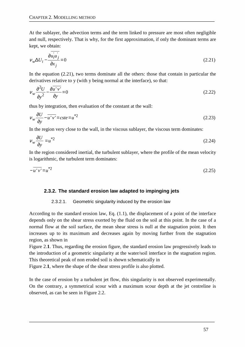
CHAPTER 2. MODELLING METHOD
57
At the sublayer, the advection terms and the term linked to pressure are most often negligible and null, respectively. That is why, for the first approximation, if only the dominant terms are kept, we obtain:
0' 'i j
w ij
u uU
x
∂∆ − =
∂ν (2.21)
In the equation (2.21), two terms dominate all the others: those that contain in particular the derivatives relative to y (with y being normal at the interface), so that:
2
20w
U u' v'
yy
∂ ∂− =∂∂
ν (2.22)
thus by integration, then evaluation of the constant at the wall:
2*w
Uu' v' cste u
y
∂ − = =∂
ν (2.23)
In the region very close to the wall, in the viscous sublayer, the viscous term dominates:
2*w
Uu
y
∂ =∂
ν (2.24)
In the region considered inertial, the turbulent sublayer, where the profile of the mean velocity is logarithmic, the turbulent term dominates:
2*u' v' u− = (2.25)
2.3.2. The standard erosion law adapted to impingin g jets
2.3.2.1. Geometric singularity induced by the erosion law According to the standard erosion law, Eq. (1.1), the displacement of a point of the interface depends only on the shear stress exerted by the fluid on the soil at this point. In the case of a normal flow at the soil surface, the mean shear stress is null at the stagnation point. It then increases up to its maximum and decreases again by moving further from the stagnation region, as shown in Figure 2.1. Thus, regarding the erosion figure, the standard erosion law progressively leads to the introduction of a geometric singularity at the water/soil interface in the stagnation region. This theoretical peak of non eroded soil is shown schematically in Figure 2.1, where the shape of the shear stress profile is also plotted. In the case of erosion by a turbulent jet flow, this singularity is not observed experimentally. On the contrary, a symmetrical scour with a maximum scour depth at the jet centreline is observed, as can be seen in Figure 2.2.
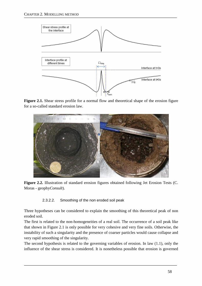
CHAPTER 2. MODELLING METHOD
58
Figure 2.1. Shear stress profile for a normal flow and theoretical shape of the erosion figure for a so-called standard erosion law.
Figure 2.2. Illustration of standard erosion figures obtained following Jet Erosion Tests (C. Moras - geophyConsult).
2.3.2.2. Smoothing of the non eroded soil peak Three hypotheses can be considered to explain the smoothing of this theoretical peak of non eroded soil. The first is related to the non-homogeneities of a real soil. The occurrence of a soil peak like that shown in Figure 2.1 is only possible for very cohesive and very fine soils. Otherwise, the instability of such a singularity and the presence of coarser particles would cause collapse and very rapid smoothing of the singularity. The second hypothesis is related to the governing variables of erosion. In law (1.1), only the influence of the shear stress is considered. It is nonetheless possible that erosion is governed
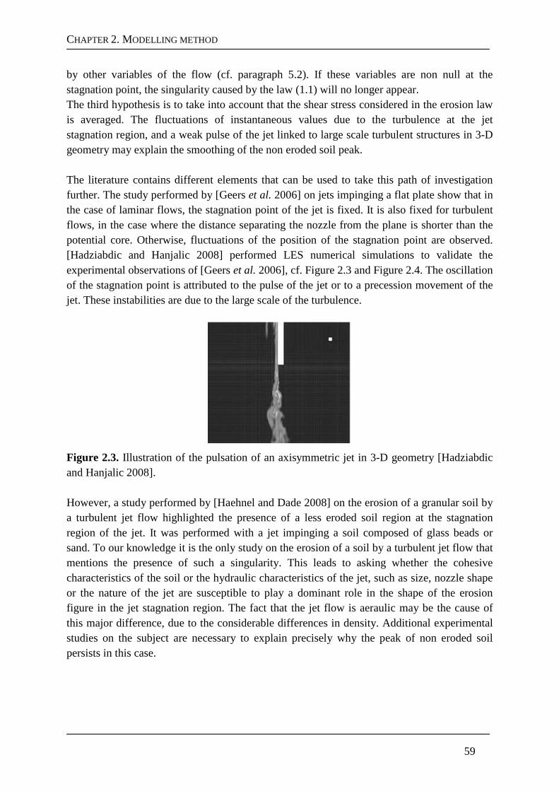
CHAPTER 2. MODELLING METHOD
59
by other variables of the flow (cf. paragraph 5.2). If these variables are non null at the stagnation point, the singularity caused by the law (1.1) will no longer appear. The third hypothesis is to take into account that the shear stress considered in the erosion law is averaged. The fluctuations of instantaneous values due to the turbulence at the jet stagnation region, and a weak pulse of the jet linked to large scale turbulent structures in 3-D geometry may explain the smoothing of the non eroded soil peak. The literature contains different elements that can be used to take this path of investigation further. The study performed by [Geers et al. 2006] on jets impinging a flat plate show that in the case of laminar flows, the stagnation point of the jet is fixed. It is also fixed for turbulent flows, in the case where the distance separating the nozzle from the plane is shorter than the potential core. Otherwise, fluctuations of the position of the stagnation point are observed. [Hadziabdic and Hanjalic 2008] performed LES numerical simulations to validate the experimental observations of [Geers et al. 2006], cf. Figure 2.3 and Figure 2.4. The oscillation of the stagnation point is attributed to the pulse of the jet or to a precession movement of the jet. These instabilities are due to the large scale of the turbulence.
Figure 2.3. Illustration of the pulsation of an axisymmetric jet in 3-D geometry [Hadziabdic and Hanjalic 2008]. However, a study performed by [Haehnel and Dade 2008] on the erosion of a granular soil by a turbulent jet flow highlighted the presence of a less eroded soil region at the stagnation region of the jet. It was performed with a jet impinging a soil composed of glass beads or sand. To our knowledge it is the only study on the erosion of a soil by a turbulent jet flow that mentions the presence of such a singularity. This leads to asking whether the cohesive characteristics of the soil or the hydraulic characteristics of the jet, such as size, nozzle shape or the nature of the jet are susceptible to play a dominant role in the shape of the erosion figure in the jet stagnation region. The fact that the jet flow is aeraulic may be the cause of this major difference, due to the considerable differences in density. Additional experimental studies on the subject are necessary to explain precisely why the peak of non eroded soil persists in this case.
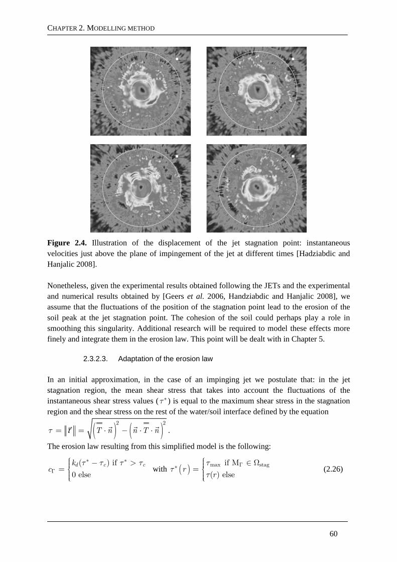
CHAPTER 2. MODELLING METHOD
60
Figure 2.4. Illustration of the displacement of the jet stagnation point: instantaneous velocities just above the plane of impingement of the jet at different times [Hadziabdic and Hanjalic 2008]. Nonetheless, given the experimental results obtained following the JETs and the experimental and numerical results obtained by [Geers et al. 2006, Handziabdic and Hanjalic 2008], we assume that the fluctuations of the position of the stagnation point lead to the erosion of the soil peak at the jet stagnation point. The cohesion of the soil could perhaps play a role in smoothing this singularity. Additional research will be required to model these effects more finely and integrate them in the erosion law. This point will be dealt with in Chapter 5.
2.3.2.3. Adaptation of the erosion law In an initial approximation, in the case of an impinging jet we postulate that: in the jet stagnation region, the mean shear stress that takes into account the fluctuations of the instantaneous shear stress values (*τ ) is equal to the maximum shear stress in the stagnation region and the shear stress on the rest of the water/soil interface defined by the equation
( ) ( )2 2
T n n T nτ= = ⋅ − ⋅ ⋅
τ .
The erosion law resulting from this simplified model is the following:
* *( ) if
0 else
d c ckc
τ τ τ τ
Γ
− >=
with ( )max stag
* if M
( ) elser
r
ττ
τ
Γ ∈ Ω=
(2.26)
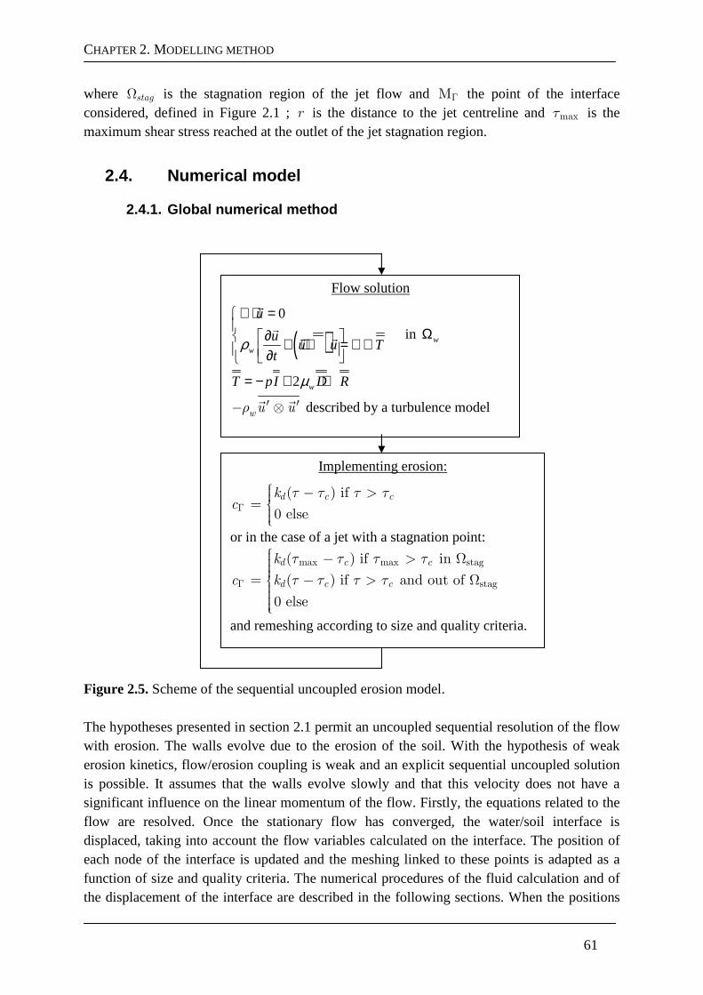
CHAPTER 2. MODELLING METHOD
61
where stagΩ is the stagnation region of the jet flow and MΓ the point of the interface considered, defined in Figure 2.1 ; r is the distance to the jet centreline and maxτ is the maximum shear stress reached at the outlet of the jet stagnation region.
2.4. Numerical model
2.4.1. Global numerical method
Figure 2.5. Scheme of the sequential uncoupled erosion model. The hypotheses presented in section 2.1 permit an uncoupled sequential resolution of the flow with erosion. The walls evolve due to the erosion of the soil. With the hypothesis of weak erosion kinetics, flow/erosion coupling is weak and an explicit sequential uncoupled solution is possible. It assumes that the walls evolve slowly and that this velocity does not have a significant influence on the linear momentum of the flow. Firstly, the equations related to the flow are resolved. Once the stationary flow has converged, the water/soil interface is displaced, taking into account the flow variables calculated on the interface. The position of each node of the interface is updated and the meshing linked to these points is adapted as a function of size and quality criteria. The numerical procedures of the fluid calculation and of the displacement of the interface are described in the following sections. When the positions
Flow solution
( )0
ρw
u
uu u T
t
∇ ⋅ =
∂ + ⋅∇ = ∇ ⋅ ∂
in wΩ
2µwT pI D R= − + +
ρwu u′ ′− ⊗
described by a turbulence model
Implementing erosion:
( ) if
0 else
d c ckc
τ τ τ τ
Γ
− >=
or in the case of a jet with a stagnation point:
max max stag
stag
( ) if in
( ) if and out of
0 else
d c c
d c c
k
c k
τ τ τ τ
τ τ τ τΓ
− > Ω= − > Ω
and remeshing according to size and quality criteria.
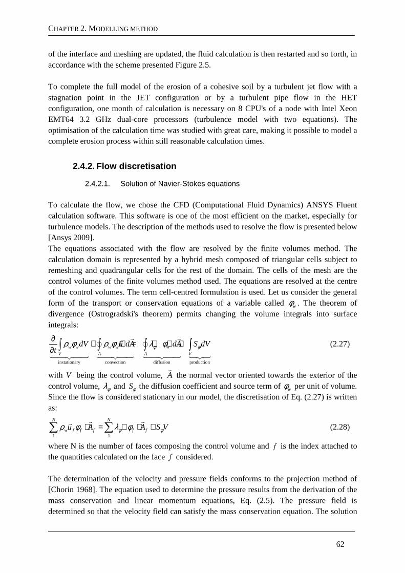
CHAPTER 2. MODELLING METHOD
62
of the interface and meshing are updated, the fluid calculation is then restarted and so forth, in accordance with the scheme presented Figure 2.5. To complete the full model of the erosion of a cohesive soil by a turbulent jet flow with a stagnation point in the JET configuration or by a turbulent pipe flow in the HET configuration, one month of calculation is necessary on 8 CPU's of a node with Intel Xeon EMT64 3.2 GHz dual-core processors (turbulence model with two equations). The optimisation of the calculation time was studied with great care, making it possible to model a complete erosion process within still reasonable calculation times.
2.4.2. Flow discretisation
2.4.2.1. Solution of Navier-Stokes equations To calculate the flow, we chose the CFD (Computational Fluid Dynamics) ANSYS Fluent calculation software. This software is one of the most efficient on the market, especially for turbulence models. The description of the methods used to resolve the flow is presented below [Ansys 2009]. The equations associated with the flow are resolved by the finite volumes method. The calculation domain is represented by a hybrid mesh composed of triangular cells subject to remeshing and quadrangular cells for the rest of the domain. The cells of the mesh are the control volumes of the finite volumes method used. The equations are resolved at the centre of the control volumes. The term cell-centred formulation is used. Let us consider the general form of the transport or conservation equations of a variable called wφ . The theorem of divergence (Ostrogradski's theorem) permits changing the volume integrals into surface integrals:
convection diffusioninstationary production
w w w w w
V A A V
dV u dA dA S dVt φ φρ φ ρ φ λ φ∂ + ⋅ = ∇ ⋅ +
∂ ∫ ∫ ∫ ∫
(2.27)
with V being the control volume, A
the normal vector oriented towards the exterior of the control volume, φλ and Sφ the diffusion coefficient and source term of wφ per unit of volume. Since the flow is considered stationary in our model, the discretisation of Eq. (2.27) is written as:
1 1φ φρ φ λ φ
N N
w f f f f fu A A S V⋅ = ∇ ⋅ +∑ ∑
(2.28)
where N is the number of faces composing the control volume and f is the index attached to the quantities calculated on the face f considered. The determination of the velocity and pressure fields conforms to the projection method of [Chorin 1968]. The equation used to determine the pressure results from the derivation of the mass conservation and linear momentum equations, Eq. (2.5). The pressure field is determined so that the velocity field can satisfy the mass conservation equation. The solution
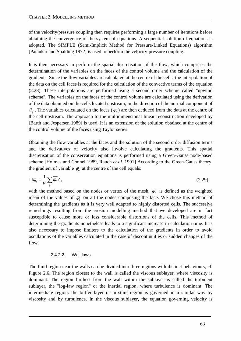
CHAPTER 2. MODELLING METHOD
63
of the velocity/pressure coupling then requires performing a large number of iterations before obtaining the convergence of the system of equations. A sequential solution of equations is adopted. The SIMPLE (Semi-Implicit Method for Pressure-Linked Equations) algorithm [Patankar and Spalding 1972] is used to perform the velocity-pressure coupling. It is then necessary to perform the spatial discretisation of the flow, which comprises the determination of the variables on the faces of the control volume and the calculation of the gradients. Since the flow variables are calculated at the centre of the cells, the interpolation of the data on the cell faces is required for the calculation of the convective terms of the equation (2.28). These interpolations are performed using a second order scheme called "upwind scheme". The variables on the faces of the control volume are calculated using the derivation of the data obtained on the cells located upstream, in the direction of the normal component of
fu
. The variables calculated on the faces (fφ ) are then deduced from the data at the centre of the cell upstream. The approach to the multidimensional linear reconstruction developed by [Barth and Jespersen 1989] is used. It is an extension of the solution obtained at the centre of the control volume of the faces using Taylor series. Obtaining the flow variables at the faces and the solution of the second order diffusion terms and the derivatives of velocity also involve calculating the gradients. This spatial discretisation of the conservation equations is performed using a Green-Gauss node-based scheme [Holmes and Connel 1989, Rauch et al. 1991] According to the Green-Gauss theory, the gradient of variable wφ at the centre of the cell equals:
1φ φw f ff
AV
∇ = ∑
(2.29)
with the method based on the nodes or vertex of the mesh, fφ is defined as the weighted mean of the values of fφ on all the nodes composing the face. We chose this method of determining the gradients as it is very well adapted to highly distorted cells. The successive remeshings resulting from the erosion modelling method that we developed are in fact susceptible to cause more or less considerable distortions of the cells. This method of determining the gradients nonetheless leads to a significant increase in calculation time. It is also necessary to impose limiters to the calculation of the gradients in order to avoid oscillations of the variables calculated in the case of discontinuities or sudden changes of the flow.
2.4.2.2. Wall laws The fluid region near the walls can be divided into three regions with distinct behaviours, cf. Figure 2.6. The region closest to the wall is called the viscous sublayer, where viscosity is dominant. The region furthest from the wall within the sublayer is called the turbulent sublayer, the "log-law region" or the inertial region, where turbulence is dominant. The intermediate region: the buffer layer or mixture region is governed in a similar way by viscosity and by turbulence. In the viscous sublayer, the equation governing velocity is
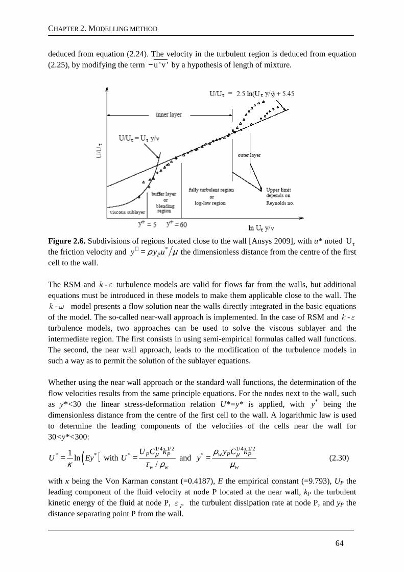
CHAPTER 2. MODELLING METHOD
64
deduced from equation (2.24). The velocity in the turbulent region is deduced from equation (2.25), by modifying the term u 'v '− by a hypothesis of length of mixture.
Figure 2.6. Subdivisions of regions located close to the wall [Ansys 2009], with u* noted
τU
the friction velocity and *Py y uρ µ+ = the dimensionless distance from the centre of the first
cell to the wall. The RSM and k -ε turbulence models are valid for flows far from the walls, but additional equations must be introduced in these models to make them applicable close to the wall. The k -ω model presents a flow solution near the walls directly integrated in the basic equations of the model. The so-called near-wall approach is implemented. In the case of RSM and k - ε turbulence models, two approaches can be used to solve the viscous sublayer and the intermediate region. The first consists in using semi-empirical formulas called wall functions. The second, the near wall approach, leads to the modification of the turbulence models in such a way as to permit the solution of the sublayer equations. Whether using the near wall approach or the standard wall functions, the determination of the flow velocities results from the same principle equations. For the nodes next to the wall, such as y*< 30 the linear stress-deformation relation U*=y* is applied, with *y being the dimensionless distance from the centre of the first cell to the wall. A logarithmic law is used to determine the leading components of the velocities of the cells near the wall for 30<y*< 300:
( )* *1lnU Ey
κ= with
1/4 1/2*
/P P
w w
U C kU µ
τ ρ= and
1/4 1/2* w P P
w
y C ky µρ
µ= (2.30)
with κ being the Von Karman constant (=0.4187), E the empirical constant (=9.793), UP the leading component of the fluid velocity at node P located at the near wall, kP the turbulent kinetic energy of the fluid at node P, Pε the turbulent dissipation rate at node P, and yP the distance separating point P from the wall.
CHAPTER 2. MODELLING METHOD
65
In the case of standard wall functions [Launder and Spalding 1972], the boundary conditions at the wall are the following:
0Pk
n
∂ =∂
,
3/4 3/2P
PP
C k
yµεκ
= (2.31)
In the near wall approach, the boundary conditions are defined differently and smoothing between the viscous and turbulent boundary layers, based on the method of [Kader 1981] is applied. Thus the term bi-layer model is used: the calculation domain is divided into two regions, a fully turbulent region and a region sensitive to viscous effects, whose delimitation is determined by:
w P Py
w
y kRe
ρµ
= (2.32)
with Rey being the turbulent Reynolds number. Standard turbulence models are used in fully turbulent flow for Rey>200. Otherwise, the one–equation approach of [Wolfshtein 1969] is used. The turbulent kinetic energy is determined using transport equations and the eddy viscosity is defined by a characteristic length lµ introduced by [Chen and Patel 1988]:
t w PC l kµ µµ ρ= , ( )Re /* 1 y AP ll y C e µ
µ−= − (2.33)
with * 3/4lC Cµκ −= and Aµ =70 constant. For RSM and k - ε turbulence models, the turbulent
dissipation rate is defined by: 3/2
Pk
l=
εε , ( )*Re /(2 )* 1 y lC
P ll y C eε−= − (2.34)
For the k-ω turbulence model, the specific dissipation rate is written in the viscous sublayer and in the "log-law region", respectively:
2
* 2
*
w i P
u
y=ω
υ β and
*
*P
U
y∞
=ωβ κ
(2.35)
with iβ and *β∞ constant.
2.4.2.3. Taking roughness into account
Taking roughness into account consists in adding a corrective term relative to roughness (∆B ) in the log law equation Eq. (2.30). Equation (2.30) becomes:
( )* *1lnκ
= −∆U Ey B (2.36)
∆B is a function of the dimensionless height of the asperities sK + defined by:
( ) 1/4 1/2s w w r µ PK K C kρ µ+ = (2.37)
with rK defined as the height of asperities expressed in meters.
CHAPTER 2. MODELLING METHOD
66
The roughness in the boundary layer can be classified into three categories. Smooth ( 2.25sK + ≤ ), transient (2.25 90sK +≤ ≤ ) and rough ( 90sK + ≥ ) regimes are considered [Cebeci and Bradshaw 1997]. For the smooth regime, 0B∆ = , otherwise the correlations related to each regime are defined empirically [Cebeci and Bradshaw 1997]. If the first cells of the mesh are located in the viscous sublayer, roughness must be taken into account directly in the geometry of the interface. For the following models, we choose the finest possible modelling of the flow variables at the interface. Given the difficulty of determining the roughness parameters, we considered the water/soil interface as a smooth wall for the first approximation. This point could be reconsidered in a future study. Indeed, according to the approach developed by [Cebeci and Bradshaw 1997], roughness starts having an effect on flow for 2.25sK + ≥ . With the results of the numerical models presented in Chapters 3 and 4 introduced in Eq. (2.37), we can estimate that if the height of the asperities exceeds 10 µmsK = , then 2.25sK + ≥ . As the JETs and HETs are performed on potentially intact real soils, the height of the asperities is effectively susceptible to exceed 10 µm .
2.4.3. Updating the position of the interface
2.4.3.1. Interface displacement code The hypothesis of slow erosion kinetics permits uncoupling resolution the flow from the erosion phenomena and permits a sequential resolution. The flow can be considered as stationary in view of the slowness of the erosion phenomena. Once the transient phase of the flow returns and the stationary regime is established, the erosion of the soil by the turbulent flow is considered. The fluid/soil interface is deformed, the mesh adapts to this deformation, the calculation starts again and so forth. To do this, we developed and implemented an interface displacement code in the ANSYS Fluent calculation software. The code we developed to model the erosion of a cohesive soil can run any erosion law coded in C/C++ language. It has been designed to be adapted to the nomenclature and rules of versions 6 to 14 of the software, for parallel resolutions, for any number of processors, and for a sequential resolution of the flow. The implementation of such a code in the software presented major difficulties linked to interactions between the code developed for the interface displacement and the software permitting the calculation of the fluid domain. These difficulties are all the greater for multiprocessor solutions of the flow and of the displacement of the interface. Nonetheless, it is necessary to parallelize the modelling method to optimise the calculation time. The numerical challenges raised by the implementation of our interface displacement code in CFD software are considerable. The first key point to be solved is to understand the system of communication between the processors, something that is not really documented. The second is the adaptation of the code for a perfect integration in the architecture of the software whose detailed operation and sources are not available. The architecture of the code that we propose is the following: i) extraction of the data obtained by the fluid domain calculation and storage in adapted structures, ii) ordering of the nodes composing the fluid/soil interface according to their position, iii) determination of the
CHAPTER 2. MODELLING METHOD
67
erosion time step, iv) determination of the position linked to each node, v) reordering according to the different processors behaviour, vi) displacement of the nodes. Once the fluid domain resolution is converged, we first extract the results obtained on the different faces of the mesh composing the water/soil interface. Given that the condition imposed is axisymmetric, the faces of the mesh composing the interface are actually edges. The calculation of the shear stress on each face is then performed. The Lagrangian displacement method used requires knowledge of the shear stress at the nodes that will be displaced. An interpolation of the shear stress obtained at the centre of the edge on two adjacent nodes of the mesh is necessary. To do this, all the information required for referencing and characterising the node of the mesh considered is stored in adapted structures. The shear stress data of the adjacent edge downstream of the node are also stored. For solutions processed in parallel, it was necessary to find a way to provide access to the data for each processor performing the flow calculations independently. The water/soil interface data extracted by the software were not gathered in an order that reflected their position on the interface, especially in the case of parallel processing. It was therefore necessary to order the nodes composing the interface. The ordering of the nodes was performed with QuickSort and fast sort algorithms. The method consists in using a pivot to partition the data sorted. An element of the table is placed in its definitive position and all the other elements are permuted so that all those lower than the pivot are placed to its left and all those higher than the pivot are placed to its right. For each sub-tables, we defined a new pivot and repeated the partitioning operation until all the elements had been sorted. It was necessary to perform a 3-D sort in the case of modelling the HET, due to the U-shaped geometry of the interface. Once the nodes are ordered according to their position on the interface, the linear interpolation of the shear stress in a mesh node is performed using the data obtained on the two faces adjacent to this node. It is then possible to determine the displacement of each node X of the interface, provided that the erosion time step has been determined beforehand t∆ . The erosion law is implemented using a first order Euler scheme:
( ) if ( , ) ( , )
0 elsed c ck t n
x t t X x t Xτ τ τ τ ∆ − >+ ∆ = +
(2.38)
Second order Adams-Bashford schemes were also used. No significant difference could be observed in the final result. The calculation time was however significantly increased, in comparison with a solution by a Euler scheme. The solution permitting the optimisation of calculation time was adopted. Initially, we determined the maximum shear stress at the interface to determine the erosion time step. Then the erosion time step was calculated in conformity with a kind of CFL condition (Courant Friedrichs Lewy), which gives the dimensional threshold below which the calculation can be seen to be unstable. If the dimension of the mesh cell is less than the
CHAPTER 2. MODELLING METHOD
68
distance travelled in the interval of the time step by the fastest wave of the equation, the error increases and invades the physical solution. To ensure optimal calculation stability, the time step is chosen so that the maximum displacement of the interface corresponds to a tenth of the size of the cells adjacent to the interface. A limiter was also implemented to ensure that the time step at time n+1 did not exceed the time step determined at time n more than 1,001 times. These values were calibrated in the case of modelling the JET performed on soil A, cf. Chapter 3. These parameters have to be calibrated for each test to maximise the optimisation of the calculation time. The establishment of other criteria can be achieved, for example, by seeking convergence. The displacement of each node of the interface is therefore known and validated to check its pertinence regarding overstepping the limits of the domain calculation. For each processor, the nodes are reordered in the order obtained during the extraction of the shear stress data. The nodes composing the water/soil interface are finally displaced. Thus the geometry of the water/soil interface is updated. Once the position of the walls has been updated, the domain is remeshed near the interface in order to discretise the domain of the calculation for this new configuration.
2.4.3.2. Remeshing The displacement of the nodes composing the interface must be followed by the displacement of all the nodes of the calculation domain near the displaced interface. To do this, the "Spring-Based Smoothing" method is used [Ansys 2009]. All the segments linking two points of the mesh are initialised as networks of interconnected springs. Before the mesh is deformed in any way, the initial spacing of the segments constitutes its state of equilibrium. The displacement of a node of the interface generates a force proportional to this displacement, affecting all the springs connected to it. The result obtained by this method is very homogeneous. According to the Hooke’s law, the force ( ijF
) applied to a node of the mesh
can be written as follows:
( )in
ij ij j ij
F k x x= ∆ − ∆∑
(2.39)
with ix∆
and jx∆
being the displacements of node i and its neighbour j, in the number of neighbouring nodes connected to i, and ijk the stiffness of the spring between nodes i and j. The stiffness between the different springs is written as:
1ij
i j
kx x
=− (2.40)
At equilibrium, the net force exerted on a point of the mesh must be null, implying the following condition:
1i
i
mnij im j
i nijj
k xx
k
+ ∆∆ =
∑
∑
(2.41)
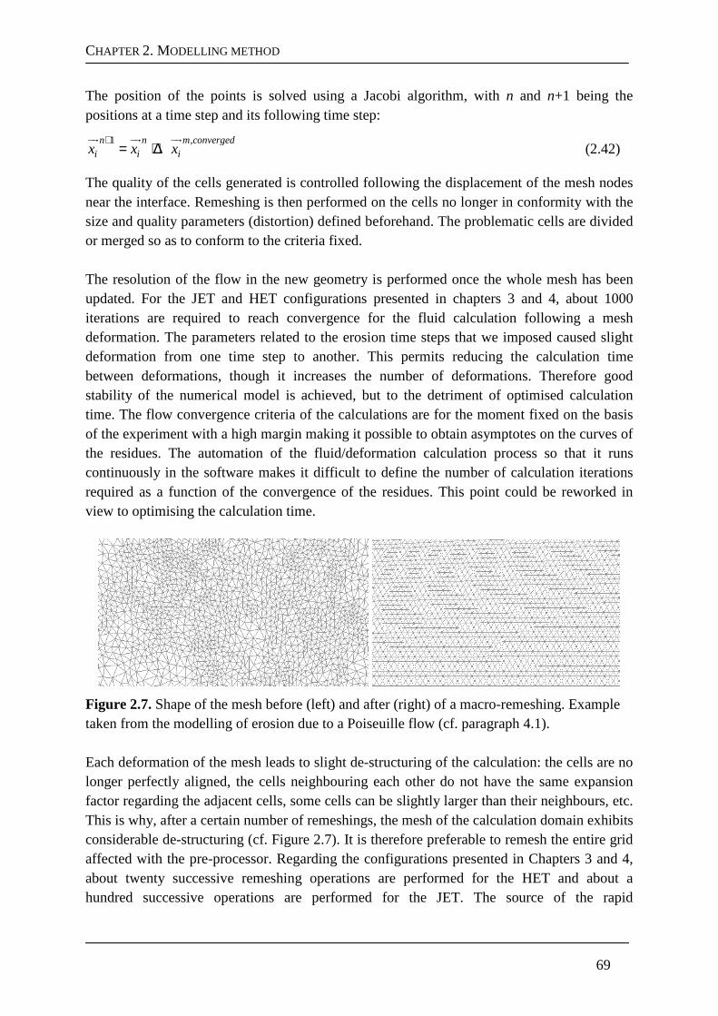
CHAPTER 2. MODELLING METHOD
69
The position of the points is solved using a Jacobi algorithm, with n and n+1 being the positions at a time step and its following time step:
1 ,n n m convergedi i ix x x
+= + ∆
(2.42)
The quality of the cells generated is controlled following the displacement of the mesh nodes near the interface. Remeshing is then performed on the cells no longer in conformity with the size and quality parameters (distortion) defined beforehand. The problematic cells are divided or merged so as to conform to the criteria fixed. The resolution of the flow in the new geometry is performed once the whole mesh has been updated. For the JET and HET configurations presented in chapters 3 and 4, about 1000 iterations are required to reach convergence for the fluid calculation following a mesh deformation. The parameters related to the erosion time steps that we imposed caused slight deformation from one time step to another. This permits reducing the calculation time between deformations, though it increases the number of deformations. Therefore good stability of the numerical model is achieved, but to the detriment of optimised calculation time. The flow convergence criteria of the calculations are for the moment fixed on the basis of the experiment with a high margin making it possible to obtain asymptotes on the curves of the residues. The automation of the fluid/deformation calculation process so that it runs continuously in the software makes it difficult to define the number of calculation iterations required as a function of the convergence of the residues. This point could be reworked in view to optimising the calculation time.
Figure 2.7. Shape of the mesh before (left) and after (right) of a macro-remeshing. Example taken from the modelling of erosion due to a Poiseuille flow (cf. paragraph 4.1). Each deformation of the mesh leads to slight de-structuring of the calculation: the cells are no longer perfectly aligned, the cells neighbouring each other do not have the same expansion factor regarding the adjacent cells, some cells can be slightly larger than their neighbours, etc. This is why, after a certain number of remeshings, the mesh of the calculation domain exhibits considerable de-structuring (cf. Figure 2.7). It is therefore preferable to remesh the entire grid affected with the pre-processor. Regarding the configurations presented in Chapters 3 and 4, about twenty successive remeshing operations are performed for the HET and about a hundred successive operations are performed for the JET. The source of the rapid
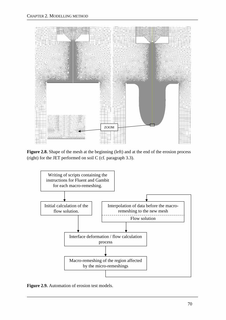
CHAPTER 2. MODELLING METHOD
70
Figure 2.8. Shape of the mesh at the beginning (left) and at the end of the erosion process (right) for the JET performed on soil C (cf. paragraph 3.3). Figure 2.9. Automation of erosion test models.
Writing of scripts containing the instructions for Fluent and Gambit
for each macro-remeshing.
Macro-remeshing of the region affected by the micro-remeshings
Initial calculation of the flow solution.
Interpolation of data before the macro-remeshing to the new mesh
Flow solution
Interface deformation / flow calculation process
ZOOM
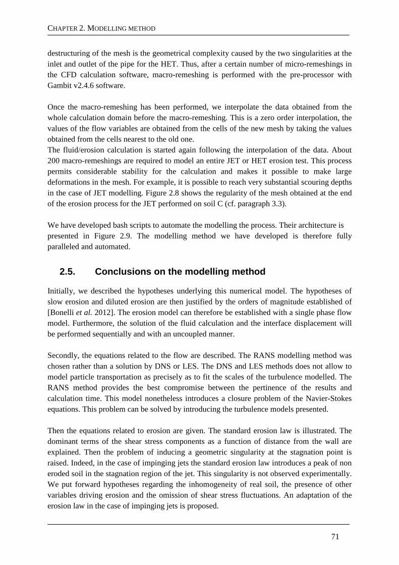
CHAPTER 2. MODELLING METHOD
71
destructuring of the mesh is the geometrical complexity caused by the two singularities at the inlet and outlet of the pipe for the HET. Thus, after a certain number of micro-remeshings in the CFD calculation software, macro-remeshing is performed with the pre-processor with Gambit v2.4.6 software. Once the macro-remeshing has been performed, we interpolate the data obtained from the whole calculation domain before the macro-remeshing. This is a zero order interpolation, the values of the flow variables are obtained from the cells of the new mesh by taking the values obtained from the cells nearest to the old one. The fluid/erosion calculation is started again following the interpolation of the data. About 200 macro-remeshings are required to model an entire JET or HET erosion test. This process permits considerable stability for the calculation and makes it possible to make large deformations in the mesh. For example, it is possible to reach very substantial scouring depths in the case of JET modelling. Figure 2.8 shows the regularity of the mesh obtained at the end of the erosion process for the JET performed on soil C (cf. paragraph 3.3). We have developed bash scripts to automate the modelling the process. Their architecture is presented in Figure 2.9. The modelling method we have developed is therefore fully paralleled and automated.
2.5. Conclusions on the modelling method
Initially, we described the hypotheses underlying this numerical model. The hypotheses of slow erosion and diluted erosion are then justified by the orders of magnitude established of [Bonelli et al. 2012]. The erosion model can therefore be established with a single phase flow model. Furthermore, the solution of the fluid calculation and the interface displacement will be performed sequentially and with an uncoupled manner. Secondly, the equations related to the flow are described. The RANS modelling method was chosen rather than a solution by DNS or LES. The DNS and LES methods does not allow to model particle transportation as precisely as to fit the scales of the turbulence modelled. The RANS method provides the best compromise between the pertinence of the results and calculation time. This model nonetheless introduces a closure problem of the Navier-Stokes equations. This problem can be solved by introducing the turbulence models presented. Then the equations related to erosion are given. The standard erosion law is illustrated. The dominant terms of the shear stress components as a function of distance from the wall are explained. Then the problem of inducing a geometric singularity at the stagnation point is raised. Indeed, in the case of impinging jets the standard erosion law introduces a peak of non eroded soil in the stagnation region of the jet. This singularity is not observed experimentally. We put forward hypotheses regarding the inhomogeneity of real soil, the presence of other variables driving erosion and the omission of shear stress fluctuations. An adaptation of the erosion law in the case of impinging jets is proposed.
CHAPTER 2. MODELLING METHOD
72
Finally, we present the numerical model with the global numerical scheme, the flow discretisation methods and the methods used to update the position of the interface. Particular attention is given to taking the wall laws into account. In addition, the interface displacement code that we have developed is described in detail. The difficulties encountered are also presented. The automation of the models is presented as is the chaining of the micro and macro remeshings and their effects. The modelling method thus formulated will be applied in chapters 3 and 4. In chapter 3, the method is applied to the model of the erosion of a cohesive soil by a jet flow with a stagnation point. The numerical results and the data of the Jet Erosion Test will be compared with the objective of concluding on the pertinence of the modelling method and the JET interpretation model. In chapter 4, the numerical model will be applied to the erosion of a cohesive soil by a laminar and turbulent pipe flow. The numerical results obtained in the case of the laminar flow will be compared to a plane Poiseuille flow. The results obtained in the case of a turbulent flow are compared with the experimental results of the Hole Erosion Test. The objective of adapting the modelling method to pipe flows is to provide additional elements to validate the method and show the method's range of applicability to relatively complex geometries.
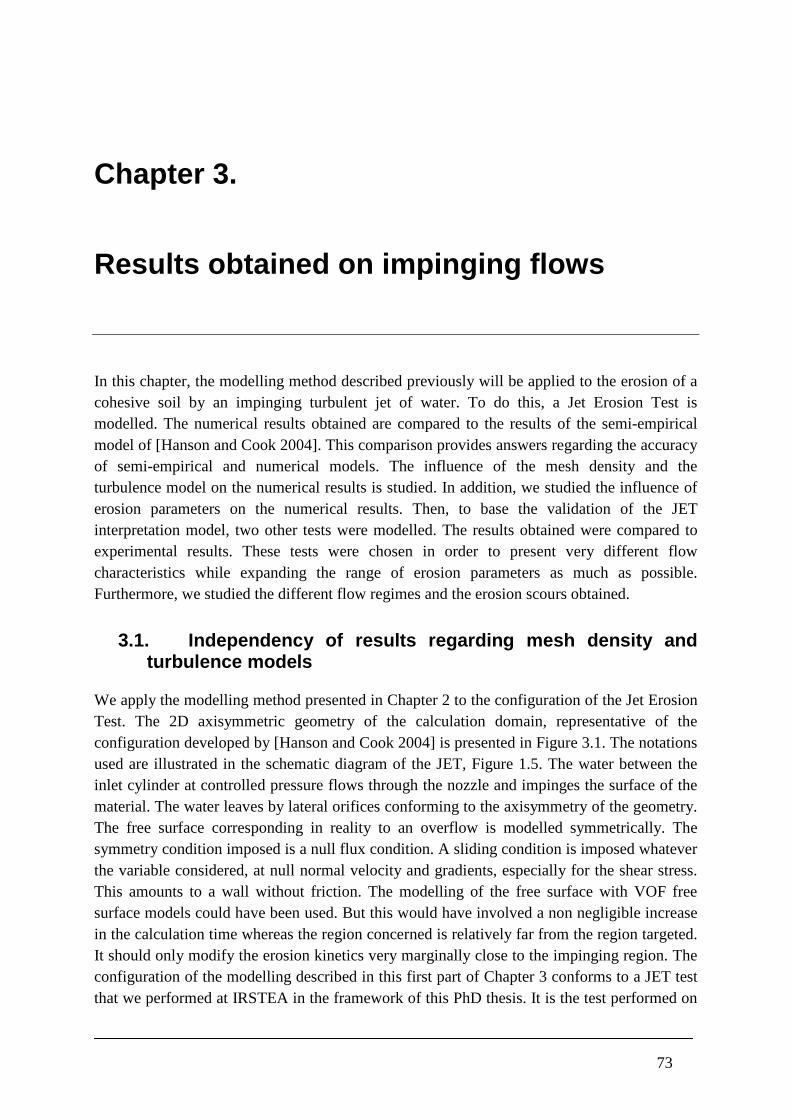
73
Chapter 3.
Results obtained on impinging flows
In this chapter, the modelling method described previously will be applied to the erosion of a cohesive soil by an impinging turbulent jet of water. To do this, a Jet Erosion Test is modelled. The numerical results obtained are compared to the results of the semi-empirical model of [Hanson and Cook 2004]. This comparison provides answers regarding the accuracy of semi-empirical and numerical models. The influence of the mesh density and the turbulence model on the numerical results is studied. In addition, we studied the influence of erosion parameters on the numerical results. Then, to base the validation of the JET interpretation model, two other tests were modelled. The results obtained were compared to experimental results. These tests were chosen in order to present very different flow characteristics while expanding the range of erosion parameters as much as possible. Furthermore, we studied the different flow regimes and the erosion scours obtained.
3.1. Independency of results regarding mesh density and turbulence models
We apply the modelling method presented in Chapter 2 to the configuration of the Jet Erosion Test. The 2D axisymmetric geometry of the calculation domain, representative of the configuration developed by [Hanson and Cook 2004] is presented in Figure 3.1. The notations used are illustrated in the schematic diagram of the JET, Figure 1.5. The water between the inlet cylinder at controlled pressure flows through the nozzle and impinges the surface of the material. The water leaves by lateral orifices conforming to the axisymmetry of the geometry. The free surface corresponding in reality to an overflow is modelled symmetrically. The symmetry condition imposed is a null flux condition. A sliding condition is imposed whatever the variable considered, at null normal velocity and gradients, especially for the shear stress. This amounts to a wall without friction. The modelling of the free surface with VOF free surface models could have been used. But this would have involved a non negligible increase in the calculation time whereas the region concerned is relatively far from the region targeted. It should only modify the erosion kinetics very marginally close to the impinging region. The configuration of the modelling described in this first part of Chapter 3 conforms to a JET test that we performed at IRSTEA in the framework of this PhD thesis. It is the test performed on
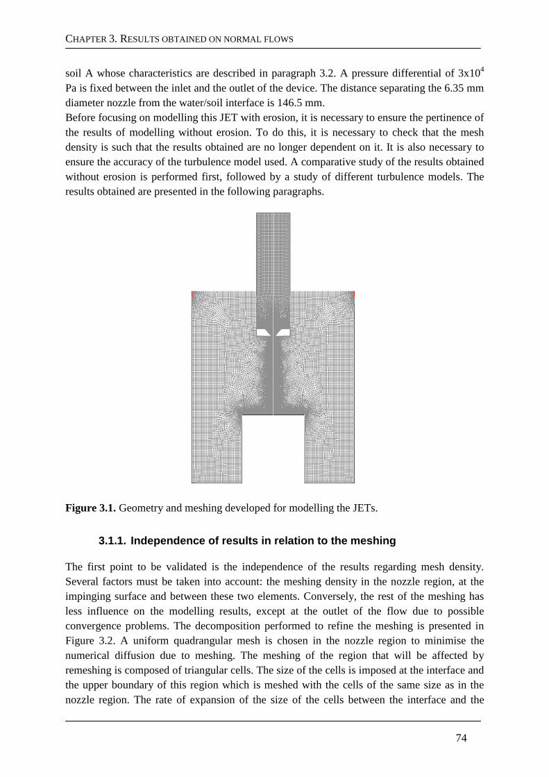
CHAPTER 3. RESULTS OBTAINED ON NORMAL FLOWS
74
soil A whose characteristics are described in paragraph 3.2. A pressure differential of 3x10⁴
Pa is fixed between the inlet and the outlet of the device. The distance separating the 6.35 mm diameter nozzle from the water/soil interface is 146.5 mm. Before focusing on modelling this JET with erosion, it is necessary to ensure the pertinence of the results of modelling without erosion. To do this, it is necessary to check that the mesh density is such that the results obtained are no longer dependent on it. It is also necessary to ensure the accuracy of the turbulence model used. A comparative study of the results obtained without erosion is performed first, followed by a study of different turbulence models. The results obtained are presented in the following paragraphs.
Figure 3.1. Geometry and meshing developed for modelling the JETs.
3.1.1. Independence of results in relation to the m eshing
The first point to be validated is the independence of the results regarding mesh density. Several factors must be taken into account: the meshing density in the nozzle region, at the impinging surface and between these two elements. Conversely, the rest of the meshing has less influence on the modelling results, except at the outlet of the flow due to possible convergence problems. The decomposition performed to refine the meshing is presented in Figure 3.2. A uniform quadrangular mesh is chosen in the nozzle region to minimise the numerical diffusion due to meshing. The meshing of the region that will be affected by remeshing is composed of triangular cells. The size of the cells is imposed at the interface and the upper boundary of this region which is meshed with the cells of the same size as in the nozzle region. The rate of expansion of the size of the cells between the interface and the
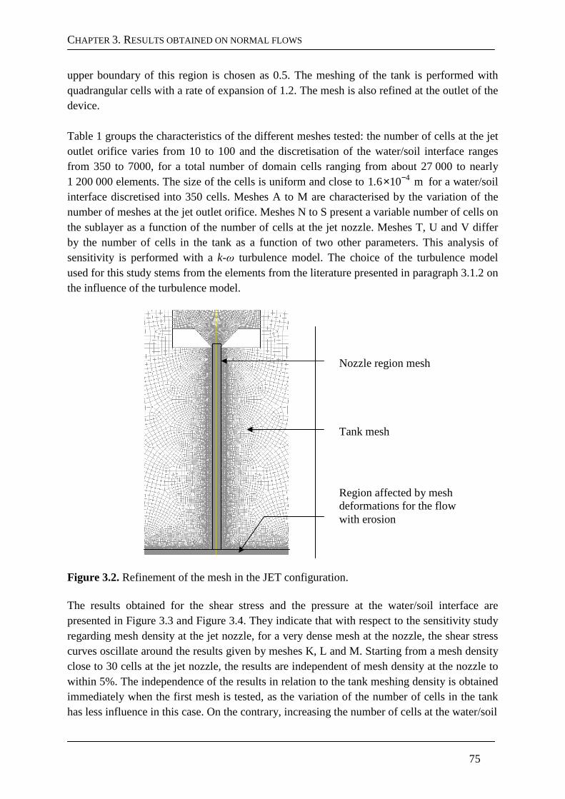
CHAPTER 3. RESULTS OBTAINED ON NORMAL FLOWS
75
upper boundary of this region is chosen as 0.5. The meshing of the tank is performed with quadrangular cells with a rate of expansion of 1.2. The mesh is also refined at the outlet of the device. Table 1 groups the characteristics of the different meshes tested: the number of cells at the jet outlet orifice varies from 10 to 100 and the discretisation of the water/soil interface ranges from 350 to 7000, for a total number of domain cells ranging from about 27 000 to nearly 1 200 000 elements. The size of the cells is uniform and close to 41 6 10 m. −× for a water/soil interface discretised into 350 cells. Meshes A to M are characterised by the variation of the number of meshes at the jet outlet orifice. Meshes N to S present a variable number of cells on the sublayer as a function of the number of cells at the jet nozzle. Meshes T, U and V differ by the number of cells in the tank as a function of two other parameters. This analysis of sensitivity is performed with a k-ω turbulence model. The choice of the turbulence model used for this study stems from the elements from the literature presented in paragraph 3.1.2 on the influence of the turbulence model.
Figure 3.2. Refinement of the mesh in the JET configuration. The results obtained for the shear stress and the pressure at the water/soil interface are presented in Figure 3.3 and Figure 3.4. They indicate that with respect to the sensitivity study regarding mesh density at the jet nozzle, for a very dense mesh at the nozzle, the shear stress curves oscillate around the results given by meshes K, L and M. Starting from a mesh density close to 30 cells at the jet nozzle, the results are independent of mesh density at the nozzle to within 5%. The independence of the results in relation to the tank meshing density is obtained immediately when the first mesh is tested, as the variation of the number of cells in the tank has less influence in this case. On the contrary, increasing the number of cells at the water/soil
Nozzle region mesh
Tank mesh
Region affected by mesh deformations for the flow with erosion
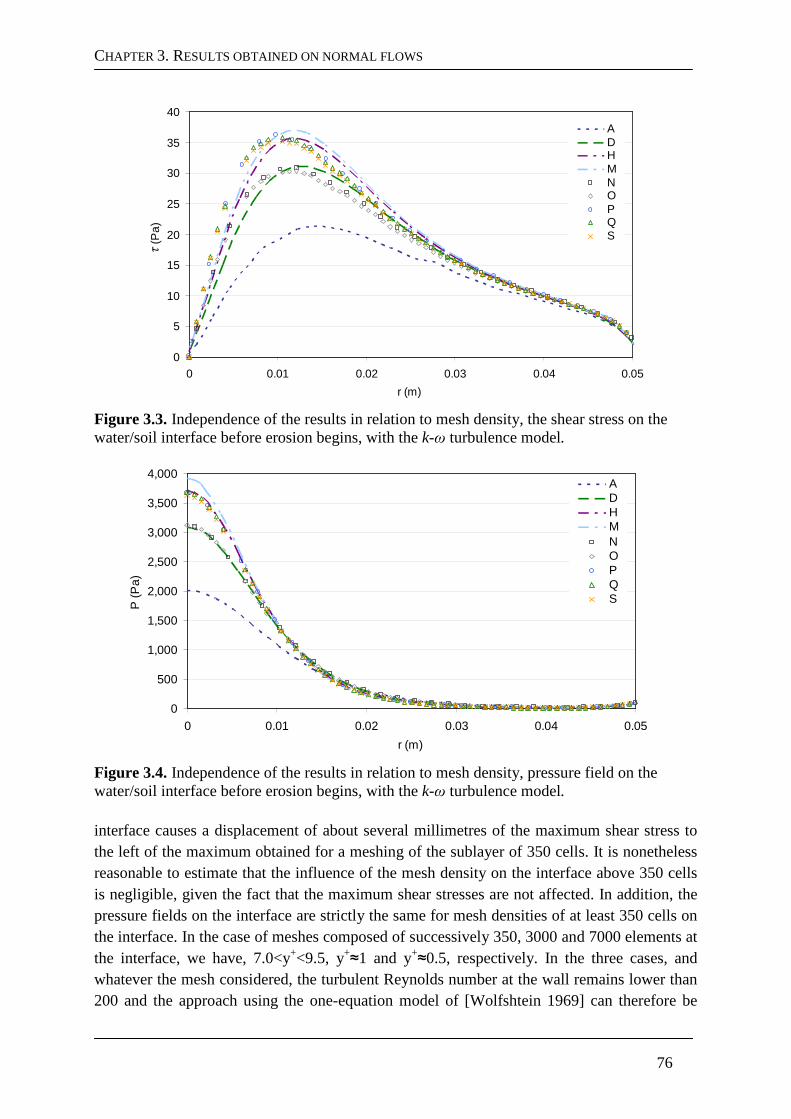
CHAPTER 3. RESULTS OBTAINED ON NORMAL FLOWS
76
0
5
10
15
20
25
30
35
40
0 0.01 0.02 0.03 0.04 0.05
r (m)
τ (P
a)
ADHMNOPQS
Figure 3.3. Independence of the results in relation to mesh density, the shear stress on the water/soil interface before erosion begins, with the k-ω turbulence model.
0
500
1,000
1,500
2,000
2,500
3,000
3,500
4,000
0 0.01 0.02 0.03 0.04 0.05
r (m)
P (P
a)
ADHMNOPQS
Figure 3.4. Independence of the results in relation to mesh density, pressure field on the water/soil interface before erosion begins, with the k-ω turbulence model. interface causes a displacement of about several millimetres of the maximum shear stress to the left of the maximum obtained for a meshing of the sublayer of 350 cells. It is nonetheless reasonable to estimate that the influence of the mesh density on the interface above 350 cells is negligible, given the fact that the maximum shear stresses are not affected. In addition, the pressure fields on the interface are strictly the same for mesh densities of at least 350 cells on the interface. In the case of meshes composed of successively 350, 3000 and 7000 elements at the interface, we have, 7.0<y+<9.5, y+≈1 and y+≈0.5, respectively. In the three cases, and whatever the mesh considered, the turbulent Reynolds number at the wall remains lower than 200 and the approach using the one-equation model of [Wolfshtein 1969] can therefore be
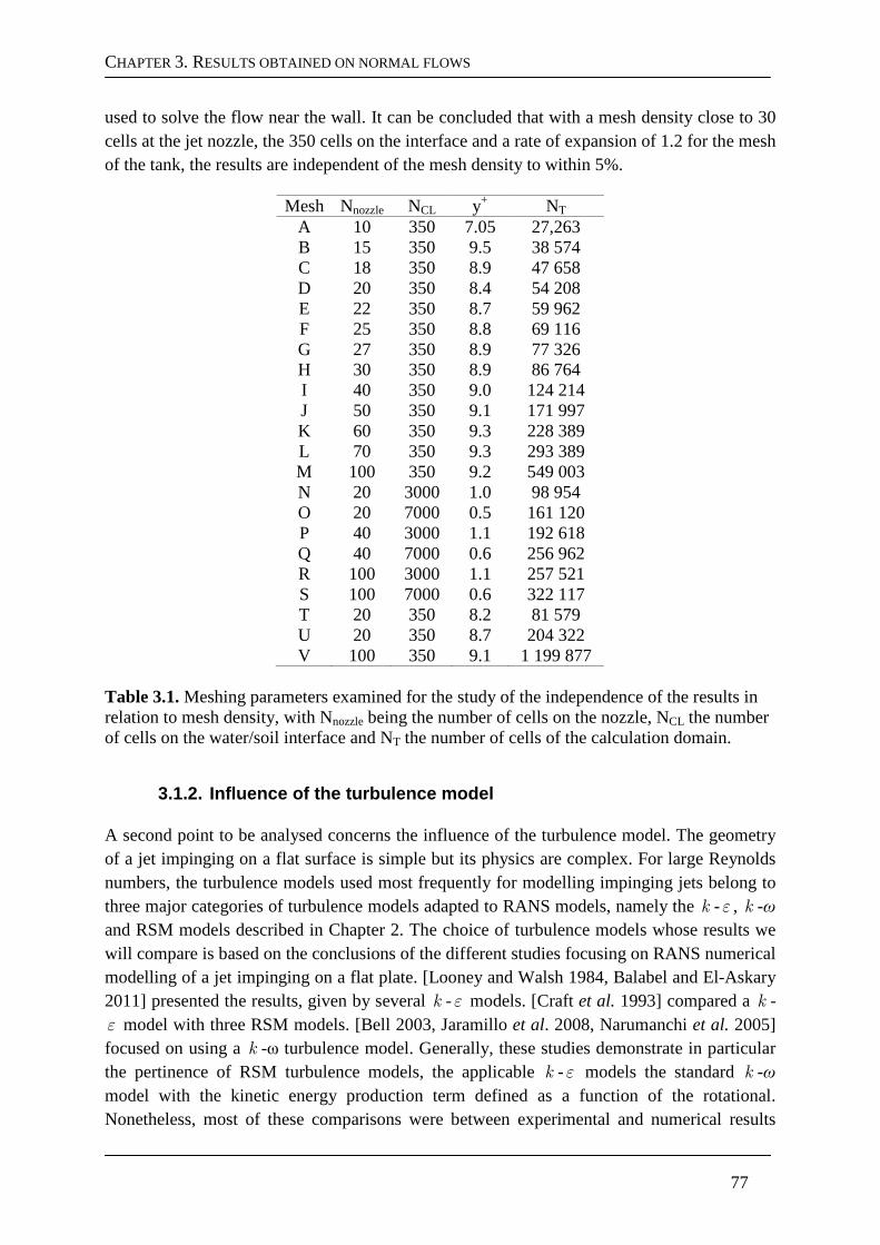
CHAPTER 3. RESULTS OBTAINED ON NORMAL FLOWS
77
used to solve the flow near the wall. It can be concluded that with a mesh density close to 30 cells at the jet nozzle, the 350 cells on the interface and a rate of expansion of 1.2 for the mesh of the tank, the results are independent of the mesh density to within 5%.
Mesh Nnozzle NCL y+ NT A 10 350 7.05 27,263 B 15 350 9.5 38 574 C 18 350 8.9 47 658 D 20 350 8.4 54 208 E 22 350 8.7 59 962 F 25 350 8.8 69 116 G 27 350 8.9 77 326 H 30 350 8.9 86 764 I 40 350 9.0 124 214 J 50 350 9.1 171 997 K 60 350 9.3 228 389 L 70 350 9.3 293 389 M 100 350 9.2 549 003 N 20 3000 1.0 98 954 O 20 7000 0.5 161 120 P 40 3000 1.1 192 618 Q 40 7000 0.6 256 962 R 100 3000 1.1 257 521 S 100 7000 0.6 322 117 T 20 350 8.2 81 579 U 20 350 8.7 204 322 V 100 350 9.1 1 199 877
Table 3.1. Meshing parameters examined for the study of the independence of the results in relation to mesh density, with Nnozzle being the number of cells on the nozzle, NCL the number of cells on the water/soil interface and NT the number of cells of the calculation domain.
3.1.2. Influence of the turbulence model
A second point to be analysed concerns the influence of the turbulence model. The geometry of a jet impinging on a flat surface is simple but its physics are complex. For large Reynolds numbers, the turbulence models used most frequently for modelling impinging jets belong to three major categories of turbulence models adapted to RANS models, namely the k -ε , k -ω and RSM models described in Chapter 2. The choice of turbulence models whose results we will compare is based on the conclusions of the different studies focusing on RANS numerical modelling of a jet impinging on a flat plate. [Looney and Walsh 1984, Balabel and El-Askary 2011] presented the results, given by several k -ε models. [Craft et al. 1993] compared a k -ε model with three RSM models. [Bell 2003, Jaramillo et al. 2008, Narumanchi et al. 2005] focused on using a k -ω turbulence model. Generally, these studies demonstrate in particular the pertinence of RSM turbulence models, the applicable k -ε models the standard k -ω model with the kinetic energy production term defined as a function of the rotational. Nonetheless, most of these comparisons were between experimental and numerical results
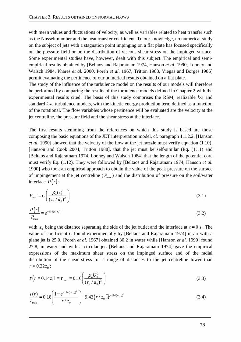
CHAPTER 3. RESULTS OBTAINED ON NORMAL FLOWS
78
with mean values and fluctuations of velocity, as well as variables related to heat transfer such as the Nusselt number and the heat transfer coefficient. To our knowledge, no numerical study on the subject of jets with a stagnation point impinging on a flat plate has focused specifically on the pressure field or on the distribution of viscous shear stress on the impinged surface. Some experimental studies have, however, dealt with this subject. The empirical and semi-empirical results obtained by [Beltaos and Rajaratnam 1974, Hanson et al. 1990, Looney and Walsch 1984, Phares et al. 2000, Poreh et al. 1967, Tritton 1988, Viegas and Borges 1986] permit evaluating the pertinence of our numerical results obtained on a flat plate. The study of the influence of the turbulence model on the results of our models will therefore be performed by comparing the results of the turbulence models defined in Chapter 2 with the experimental results cited. The basis of this study comprises the RSM, realizable k-ε and standard k-ω turbulence models, with the kinetic energy production term defined as a function of the rotational. The flow variables whose pertinence will be evaluated are the velocity at the jet centreline, the pressure field and the shear stress at the interface. The first results stemming from the references on which this study is based are those composing the basic equations of the JET interpretation model, cf. paragraph 1.1.2.2. [Hanson et al. 1990] showed that the velocity of the flow at the jet nozzle must verify equation (1.10), [Hanson and Cook 2004, Tritton 1988], that the jet must be self-similar (Eq. (1.11) and [Beltaos and Rajaratnam 1974, Looney and Walsch 1984] that the length of the potential core must verify Eq. (1.12). They were followed by [Beltaos and Rajaratnam 1974, Hanson et al. 1990] who took an empirical approach to obtain the value of the peak pressure on the surface of impingement at the jet centreline (maxP ) and the distribution of pressure on the soil/water interface ( )P r :
20
max 20 0( / )
wUP Cz d
ρ =
(3.1)
( ) 20114( / )
max
r zP re
P−= (3.2)
with 0z being the distance separating the side of the jet outlet and the interface at 0 st = . The value of coefficient C found experimentally by [Beltaos and Rajaratnam 1974] in air with a plane jet is 25.0. [Poreh et al. 1967] obtained 30.2 in water while [Hanson et al. 1990] found 27.8, in water and with a circular jet. [Beltaos and Rajaratnam 1974] gave the empirical expressions of the maximum shear stress on the impinged surface and of the radial distribution of the shear stress for a range of distances to the jet centreline lower than
00 22r . z< :
( )20
0 max 20 0
0.14 0.16( / )
wUr zz d
= = =
ρτ τ (3.3)
( )2
0 20
114( / )114( / )
0max 0
( ) 10.18 9.43 /
/
r zr zr e
r z er z
ττ
−− −= −
(3.4)
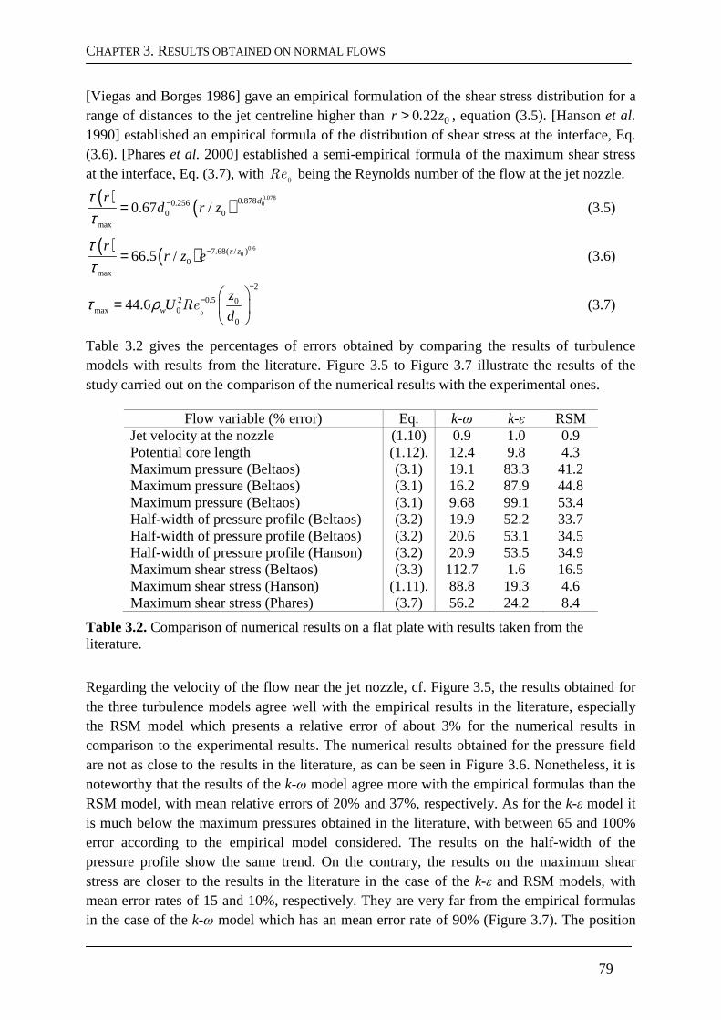
CHAPTER 3. RESULTS OBTAINED ON NORMAL FLOWS
79
[Viegas and Borges 1986] gave an empirical formulation of the shear stress distribution for a range of distances to the jet centreline higher than 00 22r . z> , equation (3.5). [Hanson et al. 1990] established an empirical formula of the distribution of shear stress at the interface, Eq. (3.6). [Phares et al. 2000] established a semi-empirical formula of the maximum shear stress at the interface, Eq. (3.7), with
0Re being the Reynolds number of the flow at the jet nozzle.
( ) ( )0.07800.8780.256
0 0max
0.67 /dr
d r zττ
−−= (3.5)
( ) ( ) 0.607.68( / )
0max
66.5 /ττ
−= r zrr z e (3.6)
0
2
2 0.5 0max 0
0
44.6 w
zU
d
−−
=
Reτ ρ (3.7)
Table 3.2 gives the percentages of errors obtained by comparing the results of turbulence models with results from the literature. Figure 3.5 to Figure 3.7 illustrate the results of the study carried out on the comparison of the numerical results with the experimental ones.
Flow variable (% error) Eq. k-ω k-ε RSM Jet velocity at the nozzle (1.10) 0.9 1.0 0.9 Potential core length (1.12). 12.4 9.8 4.3 Maximum pressure (Beltaos) (3.1) 19.1 83.3 41.2 Maximum pressure (Beltaos) (3.1) 16.2 87.9 44.8 Maximum pressure (Beltaos) (3.1) 9.68 99.1 53.4 Half-width of pressure profile (Beltaos) (3.2) 19.9 52.2 33.7 Half-width of pressure profile (Beltaos) (3.2) 20.6 53.1 34.5 Half-width of pressure profile (Hanson) (3.2) 20.9 53.5 34.9 Maximum shear stress (Beltaos) (3.3) 112.7 1.6 16.5 Maximum shear stress (Hanson) (1.11). 88.8 19.3 4.6 Maximum shear stress (Phares) (3.7) 56.2 24.2 8.4
Table 3.2. Comparison of numerical results on a flat plate with results taken from the literature.
Regarding the velocity of the flow near the jet nozzle, cf. Figure 3.5, the results obtained for the three turbulence models agree well with the empirical results in the literature, especially the RSM model which presents a relative error of about 3% for the numerical results in comparison to the experimental results. The numerical results obtained for the pressure field are not as close to the results in the literature, as can be seen in Figure 3.6. Nonetheless, it is noteworthy that the results of the k-ω model agree more with the empirical formulas than the RSM model, with mean relative errors of 20% and 37%, respectively. As for the k-ε model it is much below the maximum pressures obtained in the literature, with between 65 and 100% error according to the empirical model considered. The results on the half-width of the pressure profile show the same trend. On the contrary, the results on the maximum shear stress are closer to the results in the literature in the case of the k-ε and RSM models, with mean error rates of 15 and 10%, respectively. They are very far from the empirical formulas in the case of the k-ω model which has an mean error rate of 90% (Figure 3.7). The position
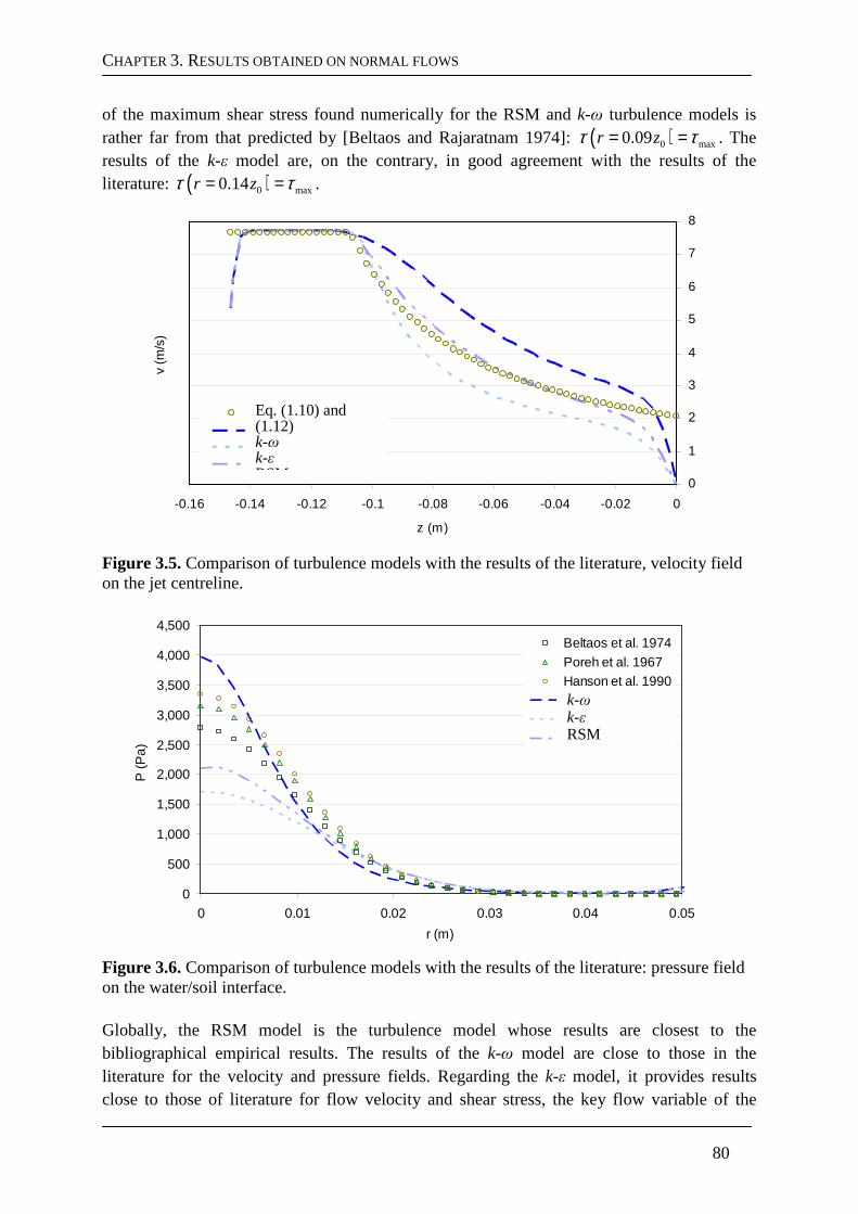
CHAPTER 3. RESULTS OBTAINED ON NORMAL FLOWS
80
of the maximum shear stress found numerically for the RSM and k-ω turbulence models is rather far from that predicted by [Beltaos and Rajaratnam 1974]: ( )0 max0.09r z= =τ τ . The results of the k-ε model are, on the contrary, in good agreement with the results of the literature: ( )0 max0.14r z= =τ τ .
0
1
2
3
4
5
6
7
8
-0.16 -0.14 -0.12 -0.1 -0.08 -0.06 -0.04 -0.02 0
z (m)
v (m
/s)
Eq. (3.2) et (3.2)k-omegak-epsilonRSM
Figure 3.5. Comparison of turbulence models with the results of the literature, velocity field on the jet centreline.
0
500
1,000
1,500
2,000
2,500
3,000
3,500
4,000
4,500
0 0.01 0.02 0.03 0.04 0.05
r (m)
P (P
a)
Beltaos et al. 1974Poreh et al. 1967Hanson et al. 1990k-omegak-epsilonRSM
Figure 3.6. Comparison of turbulence models with the results of the literature: pressure field on the water/soil interface. Globally, the RSM model is the turbulence model whose results are closest to the bibliographical empirical results. The results of the k-ω model are close to those in the literature for the velocity and pressure fields. Regarding the k-ε model, it provides results close to those of literature for flow velocity and shear stress, the key flow variable of the
k-ω k-ε RSM
Eq. (1.10) and (1.12) k-ω k-ε RSM
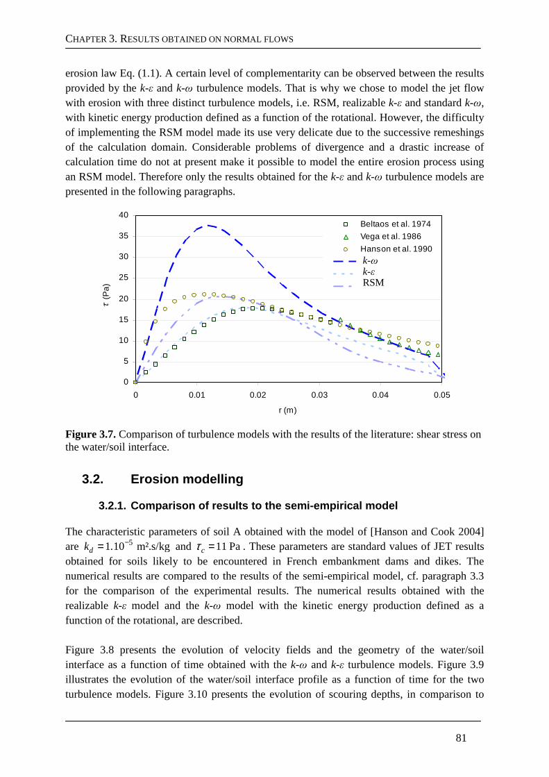
CHAPTER 3. RESULTS OBTAINED ON NORMAL FLOWS
81
erosion law Eq. (1.1). A certain level of complementarity can be observed between the results provided by the k-ε and k-ω turbulence models. That is why we chose to model the jet flow with erosion with three distinct turbulence models, i.e. RSM, realizable k-ε and standard k-ω, with kinetic energy production defined as a function of the rotational. However, the difficulty of implementing the RSM model made its use very delicate due to the successive remeshings of the calculation domain. Considerable problems of divergence and a drastic increase of calculation time do not at present make it possible to model the entire erosion process using an RSM model. Therefore only the results obtained for the k-ε and k-ω turbulence models are presented in the following paragraphs.
0
5
10
15
20
25
30
35
40
0 0.01 0.02 0.03 0.04 0.05
r (m)
τ (
Pa)
Beltaos et al. 1974
Vega et al. 1986
Hanson et al. 1990k-omega
k-epsilon
RSM
Figure 3.7. Comparison of turbulence models with the results of the literature: shear stress on the water/soil interface.
3.2. Erosion modelling
3.2.1. Comparison of results to the semi-empirical model
The characteristic parameters of soil A obtained with the model of [Hanson and Cook 2004] are 51 10 m².s/kgdk . −= and 11 Pacτ = . These parameters are standard values of JET results obtained for soils likely to be encountered in French embankment dams and dikes. The numerical results are compared to the results of the semi-empirical model, cf. paragraph 3.3 for the comparison of the experimental results. The numerical results obtained with the realizable k-ε model and the k-ω model with the kinetic energy production defined as a function of the rotational, are described. Figure 3.8 presents the evolution of velocity fields and the geometry of the water/soil interface as a function of time obtained with the k-ω and k-ε turbulence models. Figure 3.9 illustrates the evolution of the water/soil interface profile as a function of time for the two turbulence models. Figure 3.10 presents the evolution of scouring depths, in comparison to
k-ω k-ε RSM
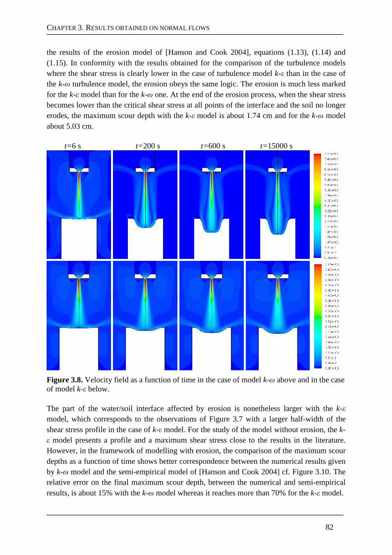
CHAPTER 3. RESULTS OBTAINED ON NORMAL FLOWS
82
the results of the erosion model of [Hanson and Cook 2004], equations (1.13), (1.14) and (1.15). In conformity with the results obtained for the comparison of the turbulence models where the shear stress is clearly lower in the case of turbulence model k-ε than in the case of the k-ω turbulence model, the erosion obeys the same logic. The erosion is much less marked for the k-ε model than for the k-ω one. At the end of the erosion process, when the shear stress becomes lower than the critical shear stress at all points of the interface and the soil no longer erodes, the maximum scour depth with the k-ε model is about 1.74 cm and for the k-ω model about 5.03 cm.
t=6 s t=200 s t=600 s t=15000 s
Figure 3.8. Velocity field as a function of time in the case of model k-ω above and in the case of model k-ε below. The part of the water/soil interface affected by erosion is nonetheless larger with the k-ε model, which corresponds to the observations of Figure 3.7 with a larger half-width of the shear stress profile in the case of k-ε model. For the study of the model without erosion, the k-ε model presents a profile and a maximum shear stress close to the results in the literature. However, in the framework of modelling with erosion, the comparison of the maximum scour depths as a function of time shows better correspondence between the numerical results given by k-ω model and the semi-empirical model of [Hanson and Cook 2004] cf. Figure 3.10. The relative error on the final maximum scour depth, between the numerical and semi-empirical results, is about 15% with the k-ω model whereas it reaches more than 70% for the k-ε model.
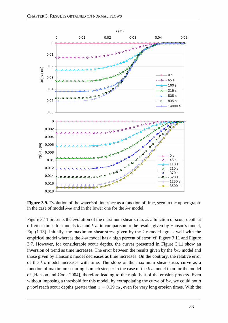
CHAPTER 3. RESULTS OBTAINED ON NORMAL FLOWS
83
0
0.01
0.02
0.03
0.04
0.05
0.06
0 0.01 0.02 0.03 0.04 0.05
r (m)
z(r)
-z0
(m)
0 s
65 s
160 s
315 s
535 s
835 s
14000 s
0
0.002
0.004
0.006
0.008
0.01
0.012
0.014
0.016
0.018
z(r)
-z0
(m)
0 s45 s110 s210 s370 s620 s1250 s8500 s
Figure 3.9. Evolution of the water/soil interface as a function of time, seen in the upper graph in the case of model k-ω and in the lower one for the k-ε model. Figure 3.11 presents the evolution of the maximum shear stress as a function of scour depth at different times for models k-ε and k-ω in comparison to the results given by Hanson's model, Eq. (1.13). Initially, the maximum shear stress given by the k-ε model agrees well with the empirical model whereas the k-ω model has a high percent of error, cf. Figure 3.11 and Figure 3.7. However, for considerable scour depths, the curves presented in Figure 3.11 show an inversion of trend as time increases. The error between the results given by the k-ω model and those given by Hanson's model decreases as time increases. On the contrary, the relative error of the k-ε model increases with time. The slope of the maximum shear stress curve as a function of maximum scouring is much steeper in the case of the k-ε model than for the model of [Hanson and Cook 2004], therefore leading to the rapid halt of the erosion process. Even without imposing a threshold for this model, by extrapolating the curve of k-ε, we could not a priori reach scour depths greater than 0.19 mz = , even for very long erosion times. With the
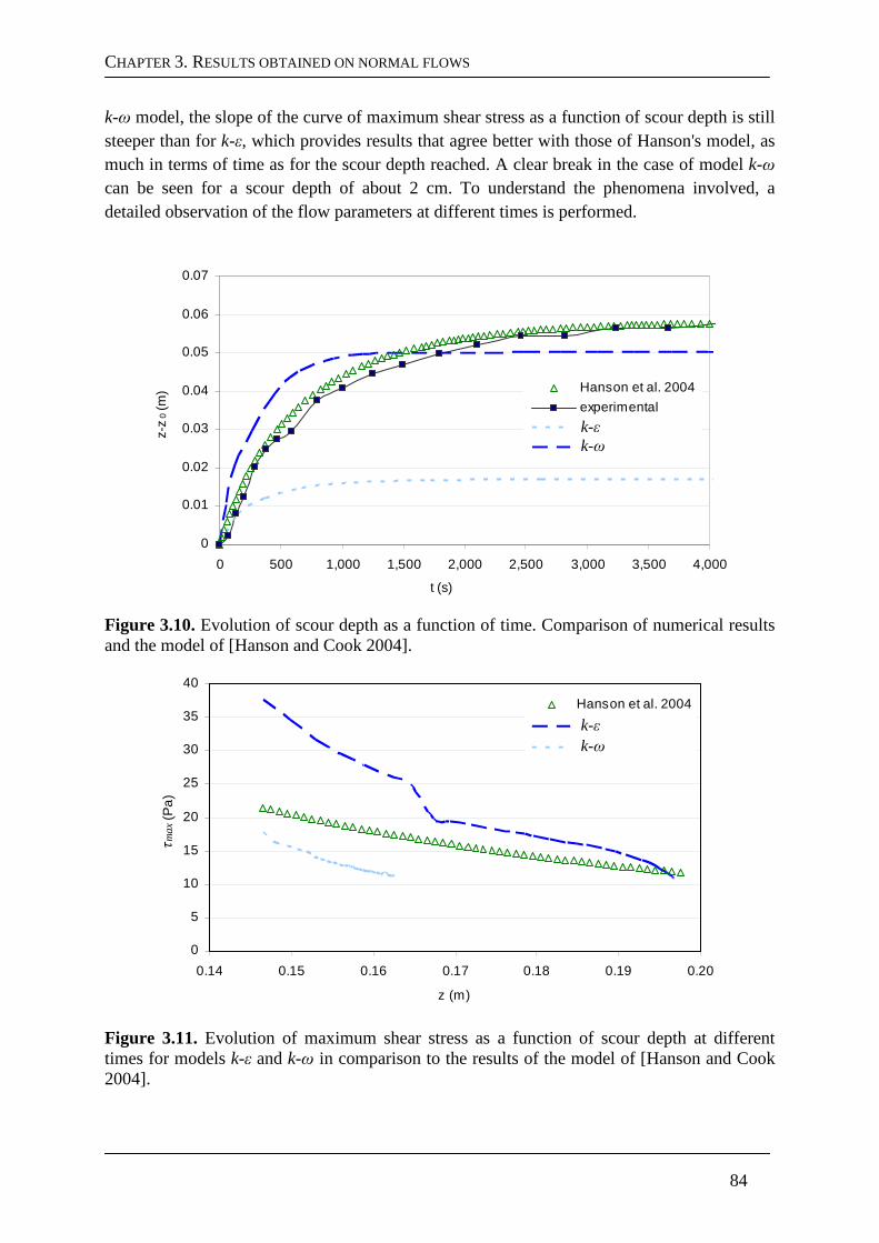
CHAPTER 3. RESULTS OBTAINED ON NORMAL FLOWS
84
k-ω model, the slope of the curve of maximum shear stress as a function of scour depth is still steeper than for k-ε, which provides results that agree better with those of Hanson's model, as much in terms of time as for the scour depth reached. A clear break in the case of model k-ω can be seen for a scour depth of about 2 cm. To understand the phenomena involved, a detailed observation of the flow parameters at different times is performed.
0
0.01
0.02
0.03
0.04
0.05
0.06
0.07
0 500 1,000 1,500 2,000 2,500 3,000 3,500 4,000
t (s)
z-z
0 (m
) Hanson et al. 2004
experimentalk-epsilon
k-omega
Figure 3.10. Evolution of scour depth as a function of time. Comparison of numerical results and the model of [Hanson and Cook 2004].
0
5
10
15
20
25
30
35
40
0.14 0.15 0.16 0.17 0.18 0.19 0.20
z (m)
τm
ax (
Pa
)
Hanson et al. 2004
k-omega
k-epsilon
Figure 3.11. Evolution of maximum shear stress as a function of scour depth at different times for models k-ε and k-ω in comparison to the results of the model of [Hanson and Cook 2004].
k-ε k-ω
k-ε k-ω
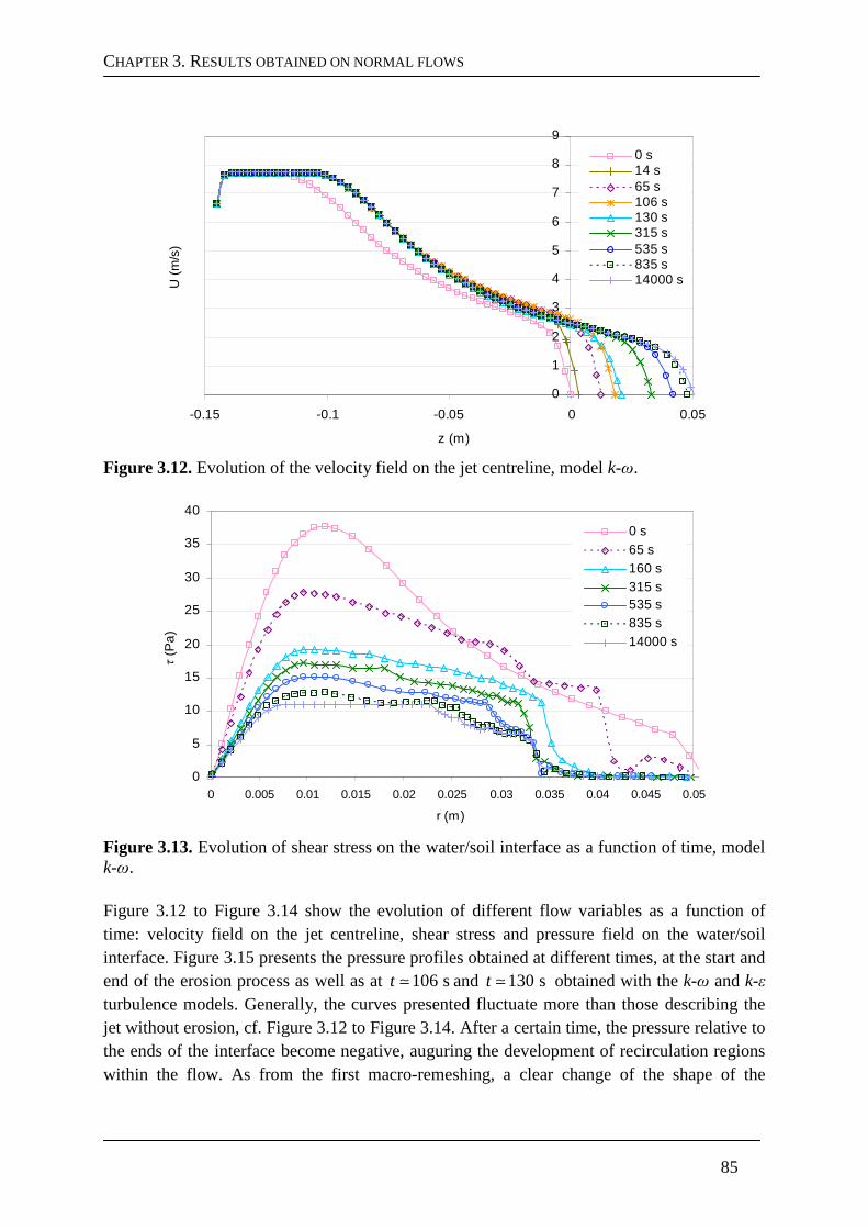
CHAPTER 3. RESULTS OBTAINED ON NORMAL FLOWS
85
0
1
2
3
4
5
6
7
8
9
-0.15 -0.1 -0.05 0 0.05
z (m)
U (
m/s
) 0 s14 s65 s106 s130 s315 s535 s835 s14000 s
Figure 3.12. Evolution of the velocity field on the jet centreline, model k-ω.
0
5
10
15
20
25
30
35
40
0 0.005 0.01 0.015 0.02 0.025 0.03 0.035 0.04 0.045 0.05
r (m)
τ (
Pa)
0 s65 s160 s315 s535 s835 s14000 s
Figure 3.13. Evolution of shear stress on the water/soil interface as a function of time, model k-ω. Figure 3.12 to Figure 3.14 show the evolution of different flow variables as a function of time: velocity field on the jet centreline, shear stress and pressure field on the water/soil interface. Figure 3.15 presents the pressure profiles obtained at different times, at the start and end of the erosion process as well as at 106 st ≃ and 130 st ≃ obtained with the k-ω and k-ε turbulence models. Generally, the curves presented fluctuate more than those describing the jet without erosion, cf. Figure 3.12 to Figure 3.14. After a certain time, the pressure relative to the ends of the interface become negative, auguring the development of recirculation regions within the flow. As from the first macro-remeshing, a clear change of the shape of the
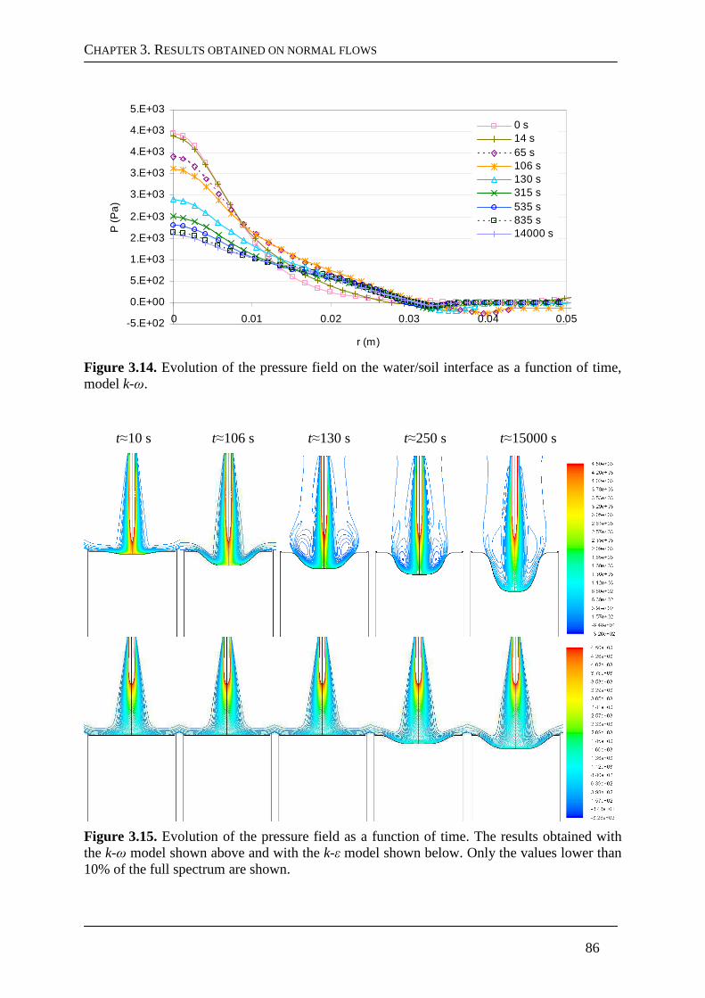
CHAPTER 3. RESULTS OBTAINED ON NORMAL FLOWS
86
-5.E+02
0.E+00
5.E+02
1.E+03
2.E+03
2.E+03
3.E+03
3.E+03
4.E+03
4.E+03
5.E+03
0 0.01 0.02 0.03 0.04 0.05
r (m)
P (
Pa
) 0 s14 s65 s106 s130 s315 s535 s835 s14000 s
Figure 3.14. Evolution of the pressure field on the water/soil interface as a function of time, model k-ω.
t≈10 s t≈106 s t≈130 s t≈250 s t≈15000 s
Figure 3.15. Evolution of the pressure field as a function of time. The results obtained with the k-ω model shown above and with the k-ε model shown below. Only the values lower than 10% of the full spectrum are shown.
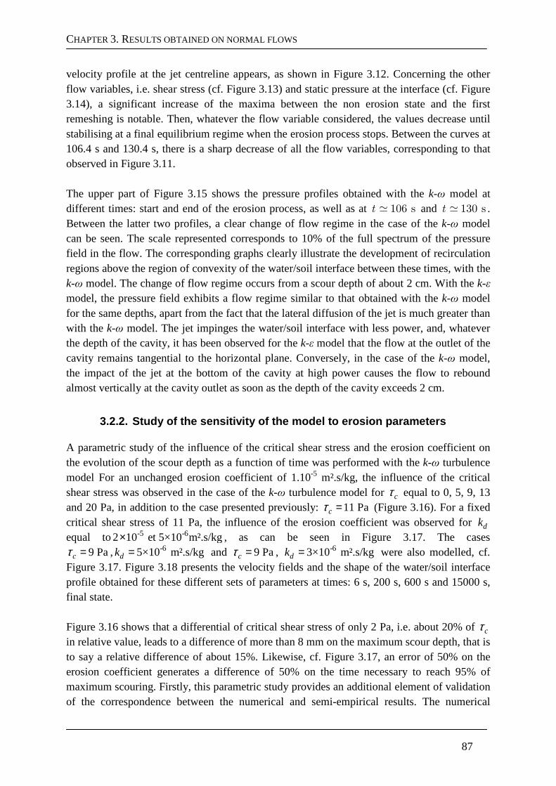
CHAPTER 3. RESULTS OBTAINED ON NORMAL FLOWS
87
velocity profile at the jet centreline appears, as shown in Figure 3.12. Concerning the other flow variables, i.e. shear stress (cf. Figure 3.13) and static pressure at the interface (cf. Figure 3.14), a significant increase of the maxima between the non erosion state and the first remeshing is notable. Then, whatever the flow variable considered, the values decrease until stabilising at a final equilibrium regime when the erosion process stops. Between the curves at 106.4 s and 130.4 s, there is a sharp decrease of all the flow variables, corresponding to that observed in Figure 3.11. The upper part of Figure 3.15 shows the pressure profiles obtained with the k-ω model at different times: start and end of the erosion process, as well as at 106 st ≃ and 130 st ≃ . Between the latter two profiles, a clear change of flow regime in the case of the k-ω model can be seen. The scale represented corresponds to 10% of the full spectrum of the pressure field in the flow. The corresponding graphs clearly illustrate the development of recirculation regions above the region of convexity of the water/soil interface between these times, with the k-ω model. The change of flow regime occurs from a scour depth of about 2 cm. With the k-ε model, the pressure field exhibits a flow regime similar to that obtained with the k-ω model for the same depths, apart from the fact that the lateral diffusion of the jet is much greater than with the k-ω model. The jet impinges the water/soil interface with less power, and, whatever the depth of the cavity, it has been observed for the k-ε model that the flow at the outlet of the cavity remains tangential to the horizontal plane. Conversely, in the case of the k-ω model, the impact of the jet at the bottom of the cavity at high power causes the flow to rebound almost vertically at the cavity outlet as soon as the depth of the cavity exceeds 2 cm.
3.2.2. Study of the sensitivity of the model to ero sion parameters
A parametric study of the influence of the critical shear stress and the erosion coefficient on the evolution of the scour depth as a function of time was performed with the k-ω turbulence model For an unchanged erosion coefficient of 1.10-5 m².s/kg, the influence of the critical shear stress was observed in the case of the k-ω turbulence model for cτ equal to 0, 5, 9, 13 and 20 Pa, in addition to the case presented previously: 11 Pacτ = (Figure 3.16). For a fixed critical shear stress of 11 Pa, the influence of the erosion coefficient was observed for dk equal to -5 -62 10 et 5×10 m².s/kg× , as can be seen in Figure 3.17. The cases
9 Pacτ = , -65×10 m².s/kgdk = and 9 Pacτ = , -63×10 m².s/kgdk = were also modelled, cf. Figure 3.17. Figure 3.18 presents the velocity fields and the shape of the water/soil interface profile obtained for these different sets of parameters at times: 6 s, 200 s, 600 s and 15000 s, final state. Figure 3.16 shows that a differential of critical shear stress of only 2 Pa, i.e. about 20% of cτ in relative value, leads to a difference of more than 8 mm on the maximum scour depth, that is to say a relative difference of about 15%. Likewise, cf. Figure 3.17, an error of 50% on the erosion coefficient generates a difference of 50% on the time necessary to reach 95% of maximum scouring. Firstly, this parametric study provides an additional element of validation of the correspondence between the numerical and semi-empirical results. The numerical
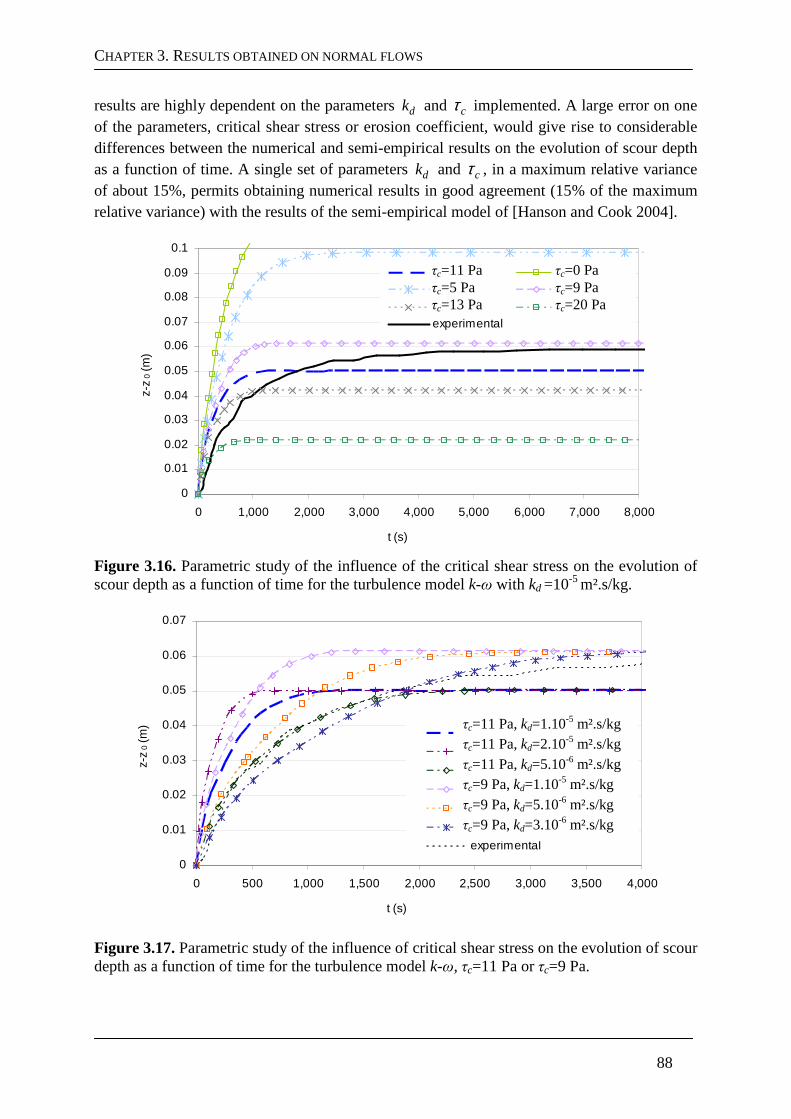
CHAPTER 3. RESULTS OBTAINED ON NORMAL FLOWS
88
results are highly dependent on the parameters dk and cτ implemented. A large error on one of the parameters, critical shear stress or erosion coefficient, would give rise to considerable differences between the numerical and semi-empirical results on the evolution of scour depth as a function of time. A single set of parameters dk and cτ , in a maximum relative variance of about 15%, permits obtaining numerical results in good agreement (15% of the maximum relative variance) with the results of the semi-empirical model of [Hanson and Cook 2004].
0
0.01
0.02
0.03
0.04
0.05
0.06
0.07
0.08
0.09
0.1
0 1,000 2,000 3,000 4,000 5,000 6,000 7,000 8,000
t (s)
z-z
0 (m
)
tauc=11Pa tauc=0Patauc=5Pa tauc=9Pa
tauc=13Pa tauc=20Paexperimental
Figure 3.16. Parametric study of the influence of the critical shear stress on the evolution of scour depth as a function of time for the turbulence model k-ω with kd =10-5 m².s/kg.
0
0.01
0.02
0.03
0.04
0.05
0.06
0.07
0 500 1,000 1,500 2,000 2,500 3,000 3,500 4,000
t (s)
z-z
0 (m
) tauc=11Pa, kd=1e-5 m²s/kg
tauc=11Pa, kd=2e-5 m²s/kg
tauc=11Pa, kd=5e-6 m²s/kg
tauc=9Pa, kd=1e-5 m²s/kg
tauc=9Pa, kd=5e-6 m²s/kg
tauc=9Pa, kd=3e-6 m²s/kg
experimental
Figure 3.17. Parametric study of the influence of critical shear stress on the evolution of scour depth as a function of time for the turbulence model k-ω, τc=11 Pa or τc=9 Pa.
τc=11 Pa τc=5 Pa τc=13 Pa
τc=11 Pa, kd=1.10-5 m².s/kg τc=11 Pa, kd=2.10-5 m².s/kg τc=11 Pa, kd=5.10-6 m².s/kg τc=9 Pa, kd=1.10-5 m².s/kg τc=9 Pa, kd=5.10-6 m².s/kg τc=9 Pa, kd=3.10-6 m².s/kg
τc=0 Pa τc=9 Pa τc=20 Pa
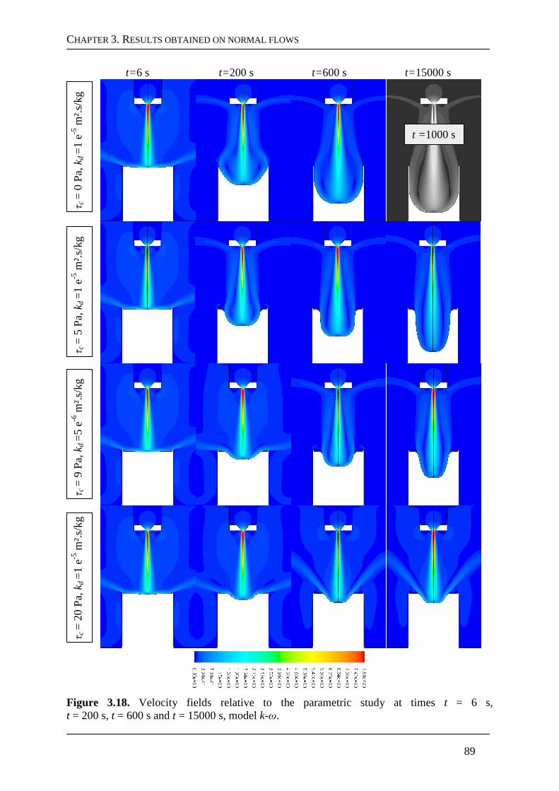
CHAPTER 3. RESULTS OBTAINED ON NORMAL FLOWS
89
t=6 s t=200 s t=600 s t=15000 s
Figure 3.18. Velocity fields relative to the parametric study at times t = 6 s, t = 200 s, t = 600 s and t = 15000 s, model k-ω.
τc =
5 P
a, k d
=1
e-5 m
².s/
kg
τc =
0 P
a, k d
=1
e-5 m
².s/
kg
t =1000 s
τc =
20
Pa,
k d =
1 e-5
m².
s/kg
τc =
9 P
a, k d
=5
e-6 m
².s/
kg
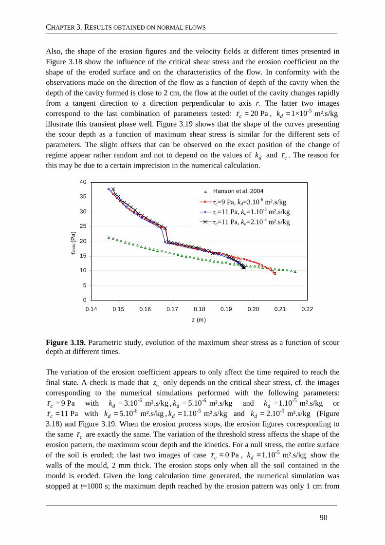
CHAPTER 3. RESULTS OBTAINED ON NORMAL FLOWS
90
Also, the shape of the erosion figures and the velocity fields at different times presented in Figure 3.18 show the influence of the critical shear stress and the erosion coefficient on the shape of the eroded surface and on the characteristics of the flow. In conformity with the observations made on the direction of the flow as a function of depth of the cavity when the depth of the cavity formed is close to 2 cm, the flow at the outlet of the cavity changes rapidly from a tangent direction to a direction perpendicular to axis r. The latter two images correspond to the last combination of parameters tested: 20 Pacτ = , -51×10 m².s/kgdk = illustrate this transient phase well. Figure 3.19 shows that the shape of the curves presenting the scour depth as a function of maximum shear stress is similar for the different sets of parameters. The slight offsets that can be observed on the exact position of the change of regime appear rather random and not to depend on the values of dk and cτ . The reason for this may be due to a certain imprecision in the numerical calculation.
0
5
10
15
20
25
30
35
40
0.14 0.15 0.16 0.17 0.18 0.19 0.20 0.21 0.22
z (m)
τm
ax (
Pa)
Hanson et al. 2004
tc9 kd3
k-omega
kd2
Figure 3.19. Parametric study, evolution of the maximum shear stress as a function of scour depth at different times. The variation of the erosion coefficient appears to only affect the time required to reach the final state. A check is made that z∞ only depends on the critical shear stress, cf. the images corresponding to the numerical simulations performed with the following parameters:
9 Pacτ = with -63.10 m².s/kgdk = , -65.10 m².s/kgdk = and -51.10 m².s/kgdk = or 11 Pacτ = with -65.10 m².s/kgdk = , -51.10 m².s/kgdk = and -52.10 m².s/kgdk = (Figure
3.18) and Figure 3.19. When the erosion process stops, the erosion figures corresponding to the same cτ are exactly the same. The variation of the threshold stress affects the shape of the erosion pattern, the maximum scour depth and the kinetics. For a null stress, the entire surface of the soil is eroded; the last two images of case 0 Pacτ = , -51.10 m².s/kgdk = show the walls of the mould, 2 mm thick. The erosion stops only when all the soil contained in the mould is eroded. Given the long calculation time generated, the numerical simulation was stopped at t=1000 s; the maximum depth reached by the erosion pattern was only 1 cm from
τc=9 Pa, kd=3.10-6 m².s/kg τc=11 Pa, kd=1.10-5 m².s/kg
τc=11 Pa, kd=2.10-5 m².s/kg
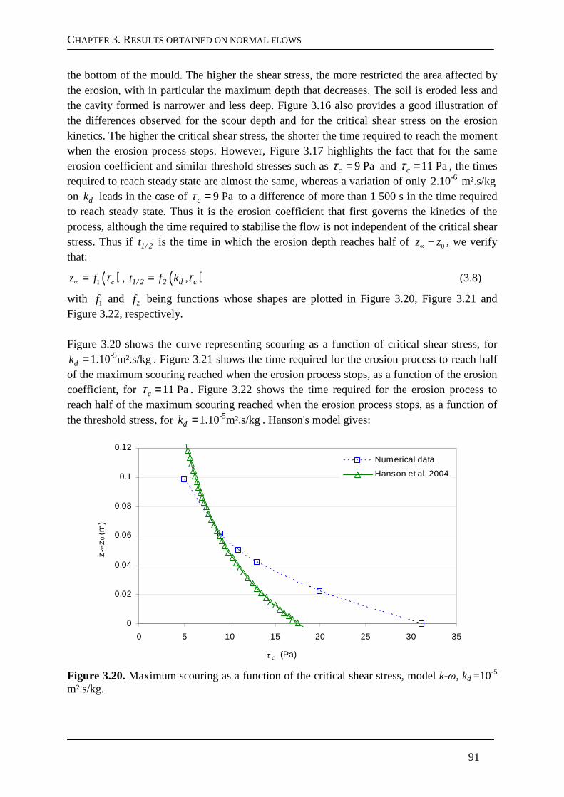
CHAPTER 3. RESULTS OBTAINED ON NORMAL FLOWS
91
the bottom of the mould. The higher the shear stress, the more restricted the area affected by the erosion, with in particular the maximum depth that decreases. The soil is eroded less and the cavity formed is narrower and less deep. Figure 3.16 also provides a good illustration of the differences observed for the scour depth and for the critical shear stress on the erosion kinetics. The higher the critical shear stress, the shorter the time required to reach the moment when the erosion process stops. However, Figure 3.17 highlights the fact that for the same erosion coefficient and similar threshold stresses such as 9 Pacτ = and 11 Pacτ = , the times required to reach steady state are almost the same, whereas a variation of only -62.10 m².s/kg on dk leads in the case of 9 Pacτ = to a difference of more than 1 500 s in the time required to reach steady state. Thus it is the erosion coefficient that first governs the kinetics of the process, although the time required to stabilise the flow is not independent of the critical shear stress. Thus if 1/ 2t is the time in which the erosion depth reaches half of 0z z∞ − , we verify that:
( )1 cz f τ∞ = , ( )1/ 2 2 d ct f k ,τ= (3.8)
with 1f and 2f being functions whose shapes are plotted in Figure 3.20, Figure 3.21 and Figure 3.22, respectively. Figure 3.20 shows the curve representing scouring as a function of critical shear stress, for
-51.10 m².s/kgdk = . Figure 3.21 shows the time required for the erosion process to reach half of the maximum scouring reached when the erosion process stops, as a function of the erosion coefficient, for 11 Pacτ = . Figure 3.22 shows the time required for the erosion process to reach half of the maximum scouring reached when the erosion process stops, as a function of the threshold stress, for -51.10 m².s/kgdk = . Hanson's model gives:
0
0.02
0.04
0.06
0.08
0.1
0.12
0 5 10 15 20 25 30 35
τ c (Pa)
z∞-z
0 (m
)
Numerical data
Hanson et al. 2004
Figure 3.20. Maximum scouring as a function of the critical shear stress, model k-ω, kd =10-5
m².s/kg.
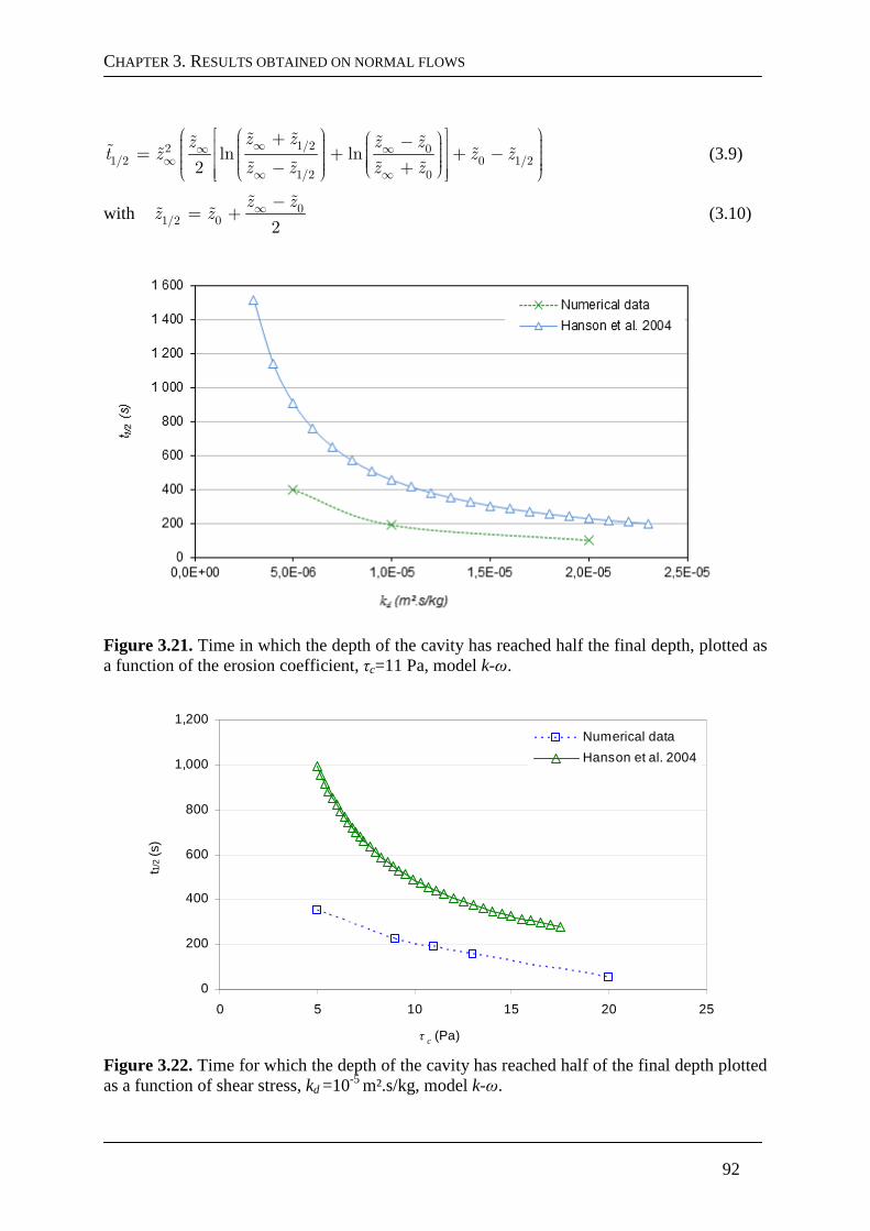
CHAPTER 3. RESULTS OBTAINED ON NORMAL FLOWS
92
1/22 01/2 0 1/2
1/2 0
ln ln2
z zz z zt z z z
z z z z
∞∞ ∞∞
∞ ∞
+ − = + + − − +
ɶ ɶɶ ɶ ɶɶ ɶ ɶ ɶ
ɶ ɶ ɶ ɶ (3.9)
with 01/2 0 2
z zz z
∞ −= +ɶ ɶ
ɶ ɶ (3.10)
Figure 3.21. Time in which the depth of the cavity has reached half the final depth, plotted as a function of the erosion coefficient, τc=11 Pa, model k-ω.
0
200
400
600
800
1,000
1,200
0 5 10 15 20 25
τ c (Pa)
t 1/2 (
s)
Numerical data
Hanson et al. 2004
Figure 3.22. Time for which the depth of the cavity has reached half of the final depth plotted as a function of shear stress, kd =10-5 m².s/kg, model k-ω.
CHAPTER 3. RESULTS OBTAINED ON NORMAL FLOWS
93
Before the beginning of the erosion process, the shear stress exerted by the fluid on the soil is much less considerable in the case of the semi-empirical model than for the numerical model, which is why the semi-empirical curve stops at much lower critical shear stresses than that of the numerical model, cf. Figure 3.20. Despite this the semi-empirical and numerical curves remain fairly close. As for the total duration of the erosion process as a function of the erosion coefficient, cf. Figure 3.21, apart from a quite considerable shift, the shape of the semi-empirical and numerical curves remain similar. The lower the values of dk , the greater the error between the numerical and semi-empirical results. The curve presenting the influence of the critical shear stress on the erosion kinetics, cf. Figure 3.22, is also very close to the results of the semi-empirical model. As with the values of dk , the lower the values of cτ , the greater the error between the numerical results and the semi-empirical results.
3.2.3. Discussion
The first element of discussion regarding the modelling of the test performed on soil A concerns the significant differences obtained for the results given by the k-ε and k-ω turbulence models. Since the k-ε models tend to diffuse too much, it can be expected that the flow variables at the interface would be attenuated for this model. If one of the two turbulence models had presented better results from the beginning to the end of the erosion process, we could have concluded that the other was less pertinent. But this is not the case here. On examining the data from the literature, the k-ε model gives better results for the maximum shear stress at the wall for a flat surface. On the other hand, after only a few macro-remeshings (hardly 5% of t∞ ), the results given by model k-ω for the scour depth (Figure 3.10), are in much better agreement with the semi-empirical and experimental results than those given by model k-ε. Nonetheless, it is well-known that model k-ε is poorly adapted to flows on curved walls [Pope 2000]. The bases for fitting its constants depend on the properties of the boundary layers on flat walls. It is difficult to call into question the results in the references on flat plates obtained by [Beltaos and Rajaratnam 1974, Hanson et al. 1990, Phares et al. 2000, Viegas and Borges 1986]. These are independent studies. The measurement methods of [Hanson 1990] and [Beltaos and Rajaratnam 1974] are distinct. The first uses a hot film probe while the second uses a Preston tube. As for the semi-empirical model of [Phares et al. 2000], it mainly relies on descriptions of the boundary layer made by [Schlichting 1960]. Also, the study performed on the influence of the turbulence model shows that a model such as the Reynolds Stress Model gives results very close to the results in the literature. For all the flow variables considered the results of the RSM fall between the results given by the k-ω model and the k-ε model, that is to say above the former and below the latter. The reliability of the results given by the RSM models is also a validation of the results in the literature whose error margin is difficult to determine. For the results given by model k-ω, when the depth of the cavity was deep enough, we could observe a major change of flow regime. In the case of the k-ε model, even for a final geometry as deep as that found with the k-ω model, no change of regime was observed. The experimental JET device did not permit observing whether such changes of flow regime occur
CHAPTER 3. RESULTS OBTAINED ON NORMAL FLOWS
94
in reality. Nonetheless, some studies carried out on the erosion of granular soils by jet flows have shown that two flow regimes can be observed as a function of the final shape of the cavity formed by the erosion. [Mazurek et al. 2001, Mazurek and Hossain 2007] reported the results of observations made by [Aderibigbe and Rajaratnam 1996, Hollick 1976, Moore and Masch 1962] on the subject of two distinct flow regimes according to the final erosion figure. If the cavity formed following the erosion process is wide and shallow, the flow regime is considered as a weakly deflected regime – WD. If the cavity formed following the erosion process is narrow and deep, the flow regime turns against itself and is considered as a strongly deflected regime – SD. [Kobus et al. 1979, O'Donoghue et al. 2001, Rouse 1939] also mention these two flow regimes. Despite strong evidence tending to validate the results given by the k-ω model, it is difficult to conclude with certainty on the better pertinence of the k-ε or k-ω models. But whatever the case, the orders of magnitude obtained for the two models tested correspond quite well to the semi-empirical model of [Hanson and Cook 2004]. The second element of discussion concerns the comparison of the numerical results with the JET interpretation model of the curves giving the maximum shear stress as a function of scour depth (Figure 3.19). In the JET interpretation model, Eq. (1.13) describes the evolution of the shear stress underlying the erosion law used. This equation is used to determine the maximum shear stress on the interface. The position of the maximum shear stress is in fact located at the outlet of the stagnation region. This value is however used to estimate the erosion at the stagnation point of the jet in both our approach and that of Hanson. Eq. (1.13) does not take account of the shape of the cavity formed by erosion. The error between the numerical and experimental results on the shear stress should therefore increase as erosion progresses. However, Figure 3.19 points to the contrary for the k-ω model. This intuitive reasoning is nonetheless valid for the numerical results obtained with the k-ε model. Also, the set of parameters 9 Pacτ = with -63.10 m².s/kgdk = , and the k-ω model, are the results of the study performed on the modelling of the JET carried out on soil A, which presents the best correspondence with the experimental and semi-empirical results. Despite adequate final kinetics and scouring, the error presented in Figure 3.19 is the same as that obtained with the initial set of parameters. Although the results obtained on the shear stress, the master variable of erosion in law (1.1), only correspond approximately, especially at the beginning of the erosion process, the evolutions of the scour depths obtained are similar. In our numerical model, the erosion law and the erosion parameters of the soil are imposed. The comparison of the results obtained with the experimental data lead to concluding on the pertinence of the erosion law with the erosion parameters obtained with the JET regarding scouring as a function of time. Given the fact that the same law is imposed in Hanson's model, the results obtained in comparison with his model only allow concluding on the pertinence of equations (1.10) to (1.13) and in the adjustment leading to the best possible fit of the erosion parameters with the experimental results. Taking into account the solid validations of the adjustment and the other equations in the literature, it is above all Eq. (1.13) that is validated by the good agreement of the results on the scour depth and the erosion kinetic energy. Despite the variances observed Figure 3.19, it appears that the precision of the shear stresses
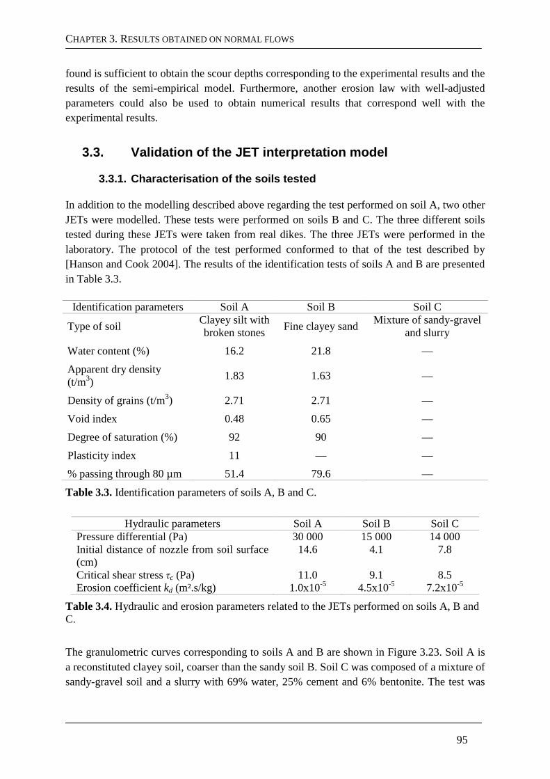
CHAPTER 3. RESULTS OBTAINED ON NORMAL FLOWS
95
found is sufficient to obtain the scour depths corresponding to the experimental results and the results of the semi-empirical model. Furthermore, another erosion law with well-adjusted parameters could also be used to obtain numerical results that correspond well with the experimental results.
3.3. Validation of the JET interpretation model
3.3.1. Characterisation of the soils tested
In addition to the modelling described above regarding the test performed on soil A, two other JETs were modelled. These tests were performed on soils B and C. The three different soils tested during these JETs were taken from real dikes. The three JETs were performed in the laboratory. The protocol of the test performed conformed to that of the test described by [Hanson and Cook 2004]. The results of the identification tests of soils A and B are presented in Table 3.3.
Identification parameters Soil A Soil B Soil C
Type of soil Clayey silt with broken stones
Fine clayey sand Mixture of sandy-gravel
and slurry
Water content (%) 16.2 21.8 —
Apparent dry density (t/m3)
1.83 1.63 —
Density of grains (t/m3) 2.71 2.71 —
Void index 0.48 0.65 —
Degree of saturation (%) 92 90 —
Plasticity index 11 — —
% passing through 80 µm 51.4 79.6 —
Table 3.3. Identification parameters of soils A, B and C.
Hydraulic parameters Soil A Soil B Soil C
Pressure differential (Pa) 30 000 15 000 14 000 Initial distance of nozzle from soil surface (cm)
14.6 4.1 7.8
Critical shear stress τc (Pa) 11.0 9.1 8.5 Erosion coefficient kd (m².s/kg) 1.0x10⁻⁵ 4.5x10⁻⁵ 7.2x10⁻⁵
Table 3.4. Hydraulic and erosion parameters related to the JETs performed on soils A, B and C.
The granulometric curves corresponding to soils A and B are shown in Figure 3.23. Soil A is a reconstituted clayey soil, coarser than the sandy soil B. Soil C was composed of a mixture of sandy-gravel soil and a slurry with 69% water, 25% cement and 6% bentonite. The test was
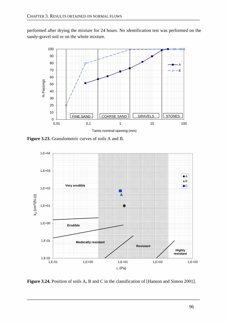
CHAPTER 3. RESULTS OBTAINED ON NORMAL FLOWS
96
performed after drying the mixture for 24 hours. No identification test was performed on the sandy-gravel soil or on the whole mixture.
0
10
20
30
40
50
60
70
80
90
100
0,01 0,1 1 10 100
% P
assi
ngs
Tamis nominal opening (mm)
A
B
FINE SAND COARSE SAND GRAVELS STONES
Figure 3.23. Granulometric curves of soils A and B.
1,E-02
1,E-01
1,E+00
1,E+01
1,E+02
1,E+03
1,E+04
1,E-01 1,E+00 1,E+01 1,E+02 1,E+03
k d(c
m3 /
(N.s
))
τc (Pa)
A
B
C
Moderatly resistantResistant
Highlyresistant
Erodible
Very erodible
Figure 3.24. Position of soils A, B and C in the classification of [Hanson and Simon 2001].
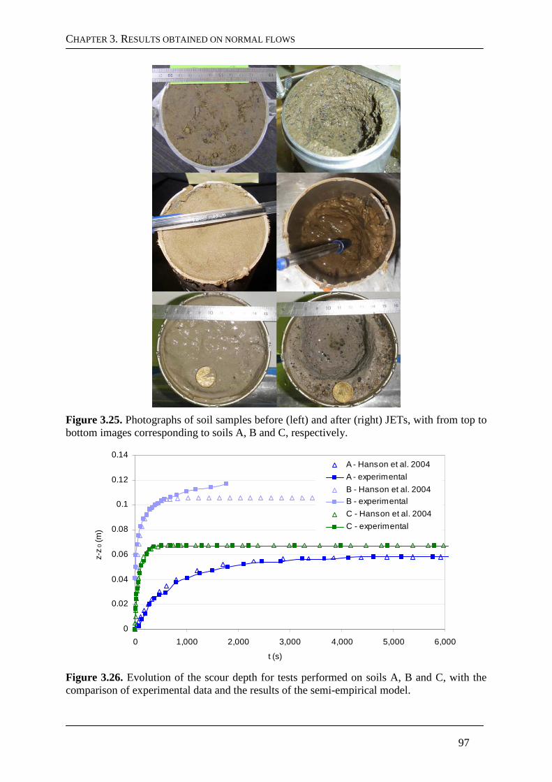
CHAPTER 3. RESULTS OBTAINED ON NORMAL FLOWS
97
Figure 3.25. Photographs of soil samples before (left) and after (right) JETs, with from top to bottom images corresponding to soils A, B and C, respectively.
0
0.02
0.04
0.06
0.08
0.1
0.12
0.14
0 1,000 2,000 3,000 4,000 5,000 6,000
t (s)
z-z
0 (m
)
A - Hanson et al. 2004
A - experimental
B - Hanson et al. 2004B - experimental
C - Hanson et al. 2004
C - experimental
Figure 3.26. Evolution of the scour depth for tests performed on soils A, B and C, with the comparison of experimental data and the results of the semi-empirical model.
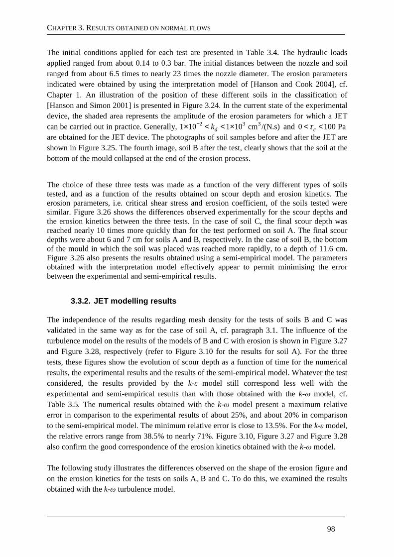
CHAPTER 3. RESULTS OBTAINED ON NORMAL FLOWS
98
The initial conditions applied for each test are presented in Table 3.4. The hydraulic loads applied ranged from about 0.14 to 0.3 bar. The initial distances between the nozzle and soil ranged from about 6.5 times to nearly 23 times the nozzle diameter. The erosion parameters indicated were obtained by using the interpretation model of [Hanson and Cook 2004], cf. Chapter 1. An illustration of the position of these different soils in the classification of [Hanson and Simon 2001] is presented in Figure 3.24. In the current state of the experimental device, the shaded area represents the amplitude of the erosion parameters for which a JET can be carried out in practice. Generally, 2 3 31 10 1 10 cm /(N.s)dk−× < < × and 0 100 Pac< <τ are obtained for the JET device. The photographs of soil samples before and after the JET are shown in Figure 3.25. The fourth image, soil B after the test, clearly shows that the soil at the bottom of the mould collapsed at the end of the erosion process.
The choice of these three tests was made as a function of the very different types of soils tested, and as a function of the results obtained on scour depth and erosion kinetics. The erosion parameters, i.e. critical shear stress and erosion coefficient, of the soils tested were similar. Figure 3.26 shows the differences observed experimentally for the scour depths and the erosion kinetics between the three tests. In the case of soil C, the final scour depth was reached nearly 10 times more quickly than for the test performed on soil A. The final scour depths were about 6 and 7 cm for soils A and B, respectively. In the case of soil B, the bottom of the mould in which the soil was placed was reached more rapidly, to a depth of 11.6 cm. Figure 3.26 also presents the results obtained using a semi-empirical model. The parameters obtained with the interpretation model effectively appear to permit minimising the error between the experimental and semi-empirical results.
3.3.2. JET modelling results
The independence of the results regarding mesh density for the tests of soils B and C was validated in the same way as for the case of soil A, cf. paragraph 3.1. The influence of the turbulence model on the results of the models of B and C with erosion is shown in Figure 3.27 and Figure 3.28, respectively (refer to Figure 3.10 for the results for soil A). For the three tests, these figures show the evolution of scour depth as a function of time for the numerical results, the experimental results and the results of the semi-empirical model. Whatever the test considered, the results provided by the k-ε model still correspond less well with the experimental and semi-empirical results than with those obtained with the k-ω model, cf. Table 3.5. The numerical results obtained with the k-ω model present a maximum relative error in comparison to the experimental results of about 25%, and about 20% in comparison to the semi-empirical model. The minimum relative error is close to 13.5%. For the k-ε model, the relative errors range from 38.5% to nearly 71%. Figure 3.10, Figure 3.27 and Figure 3.28 also confirm the good correspondence of the erosion kinetics obtained with the k-ω model. The following study illustrates the differences observed on the shape of the erosion figure and on the erosion kinetics for the tests on soils A, B and C. To do this, we examined the results obtained with the k-ω turbulence model.
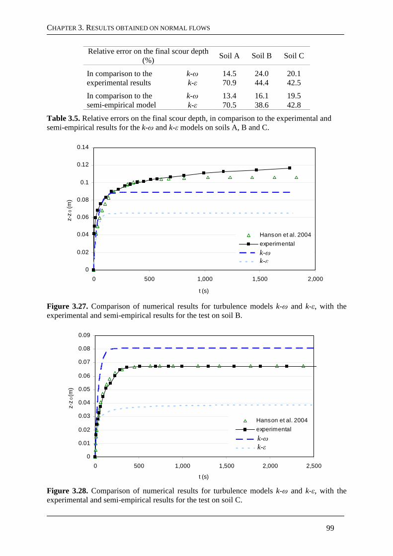
CHAPTER 3. RESULTS OBTAINED ON NORMAL FLOWS
99
Relative error on the final scour depth (%)
Soil A Soil B Soil C
In comparison to the experimental results
k-ω 14.5 24.0 20.1 k-ε 70.9 44.4 42.5
In comparison to the semi-empirical model
k-ω 13.4 16.1 19.5 k-ε 70.5 38.6 42.8
Table 3.5. Relative errors on the final scour depth, in comparison to the experimental and semi-empirical results for the k-ω and k-ε models on soils A, B and C.
0
0.02
0.04
0.06
0.08
0.1
0.12
0.14
0 500 1,000 1,500 2,000
t (s)
z-z
0 (m
)
Hanson et al. 2004
experimentalk-omega
k-epsilon
Figure 3.27. Comparison of numerical results for turbulence models k-ω and k-ε, with the experimental and semi-empirical results for the test on soil B.
0
0.01
0.02
0.03
0.04
0.05
0.06
0.07
0.08
0.09
0 500 1,000 1,500 2,000 2,500
t (s)
z-z
0 (m
)
Hanson et al. 2004
experimental
k-omega
k-epsilon
Figure 3.28. Comparison of numerical results for turbulence models k-ω and k-ε, with the experimental and semi-empirical results for the test on soil C.
k-ω k-ε
k-ω k-ε
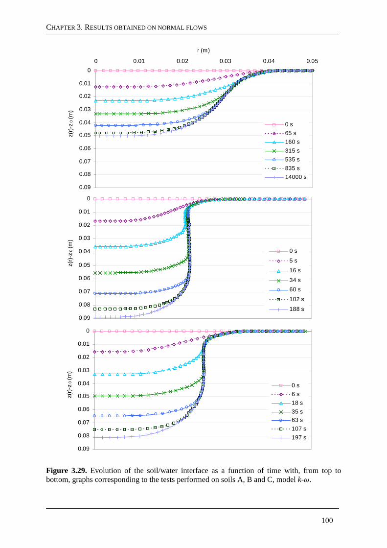
CHAPTER 3. RESULTS OBTAINED ON NORMAL FLOWS
100
0
0.01
0.02
0.03
0.04
0.05
0.06
0.07
0.08
0.09
0 0.01 0.02 0.03 0.04 0.05
r (m)
z(r)
-z0
(m)
0 s
65 s
160 s
315 s
535 s
835 s
14000 s
0
0.01
0.02
0.03
0.04
0.05
0.06
0.07
0.08
0.09
0 0.01 0.02 0.03 0.04 0.05
z(r)
-z0
(m)
0 s
5 s
16 s
34 s
60 s
102 s
188 s
0
0.01
0.02
0.03
0.04
0.05
0.06
0.07
0.08
0.09
z(r)
-z0 (
m)
0 s
6 s
18 s
35 s63 s
107 s
197 s
Figure 3.29. Evolution of the soil/water interface as a function of time with, from top to bottom, graphs corresponding to the tests performed on soils A, B and C, model k-ω.
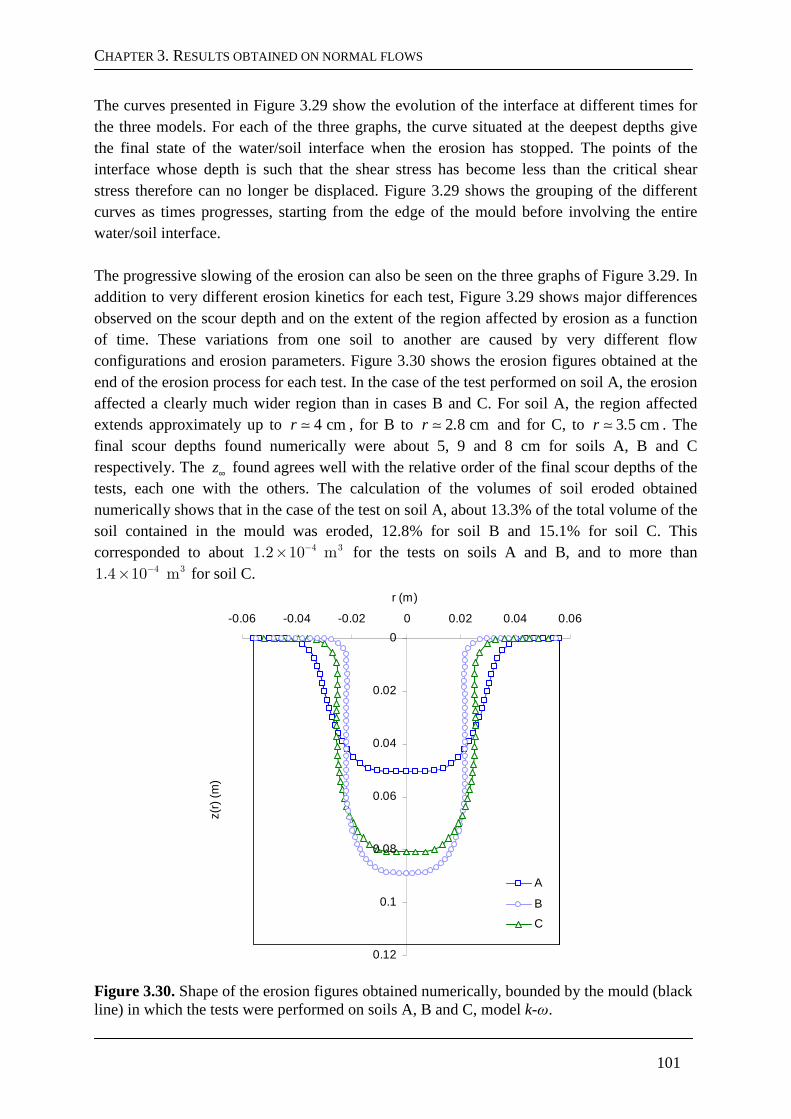
CHAPTER 3. RESULTS OBTAINED ON NORMAL FLOWS
101
The curves presented in Figure 3.29 show the evolution of the interface at different times for the three models. For each of the three graphs, the curve situated at the deepest depths give the final state of the water/soil interface when the erosion has stopped. The points of the interface whose depth is such that the shear stress has become less than the critical shear stress therefore can no longer be displaced. Figure 3.29 shows the grouping of the different curves as times progresses, starting from the edge of the mould before involving the entire water/soil interface. The progressive slowing of the erosion can also be seen on the three graphs of Figure 3.29. In addition to very different erosion kinetics for each test, Figure 3.29 shows major differences observed on the scour depth and on the extent of the region affected by erosion as a function of time. These variations from one soil to another are caused by very different flow configurations and erosion parameters. Figure 3.30 shows the erosion figures obtained at the end of the erosion process for each test. In the case of the test performed on soil A, the erosion affected a clearly much wider region than in cases B and C. For soil A, the region affected extends approximately up to 4 cmr ≃ , for B to 2 8 cmr .≃ and for C, to 3 5 cmr .≃ . The final scour depths found numerically were about 5, 9 and 8 cm for soils A, B and C respectively. The z∞ found agrees well with the relative order of the final scour depths of the tests, each one with the others. The calculation of the volumes of soil eroded obtained numerically shows that in the case of the test on soil A, about 13.3% of the total volume of the soil contained in the mould was eroded, 12.8% for soil B and 15.1% for soil C. This corresponded to about 4 31.2 10 m−× for the tests on soils A and B, and to more than
4 31.4 10 m−× for soil C.
0
0.02
0.04
0.06
0.08
0.1
0.12
-0.06 -0.04 -0.02 0 0.02 0.04 0.06
r (m)
z(r)
(m)
A
B
C
Figure 3.30. Shape of the erosion figures obtained numerically, bounded by the mould (black line) in which the tests were performed on soils A, B and C, model k-ω.
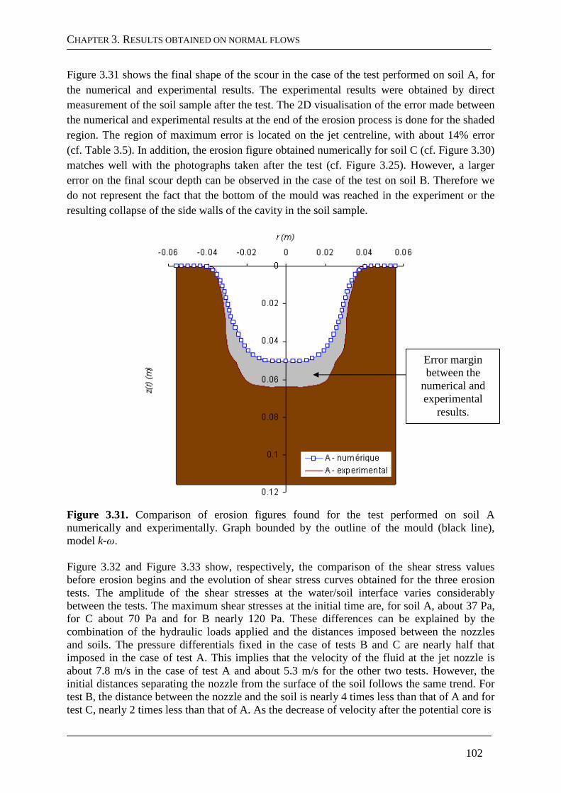
CHAPTER 3. RESULTS OBTAINED ON NORMAL FLOWS
102
Figure 3.31 shows the final shape of the scour in the case of the test performed on soil A, for the numerical and experimental results. The experimental results were obtained by direct measurement of the soil sample after the test. The 2D visualisation of the error made between the numerical and experimental results at the end of the erosion process is done for the shaded region. The region of maximum error is located on the jet centreline, with about 14% error (cf. Table 3.5). In addition, the erosion figure obtained numerically for soil C (cf. Figure 3.30) matches well with the photographs taken after the test (cf. Figure 3.25). However, a larger error on the final scour depth can be observed in the case of the test on soil B. Therefore we do not represent the fact that the bottom of the mould was reached in the experiment or the resulting collapse of the side walls of the cavity in the soil sample.
Figure 3.31. Comparison of erosion figures found for the test performed on soil A numerically and experimentally. Graph bounded by the outline of the mould (black line), model k-ω. Figure 3.32 and Figure 3.33 show, respectively, the comparison of the shear stress values before erosion begins and the evolution of shear stress curves obtained for the three erosion tests. The amplitude of the shear stresses at the water/soil interface varies considerably between the tests. The maximum shear stresses at the initial time are, for soil A, about 37 Pa, for C about 70 Pa and for B nearly 120 Pa. These differences can be explained by the combination of the hydraulic loads applied and the distances imposed between the nozzles and soils. The pressure differentials fixed in the case of tests B and C are nearly half that imposed in the case of test A. This implies that the velocity of the fluid at the jet nozzle is about 7.8 m/s in the case of test A and about 5.3 m/s for the other two tests. However, the initial distances separating the nozzle from the surface of the soil follows the same trend. For test B, the distance between the nozzle and the soil is nearly 4 times less than that of A and for test C, nearly 2 times less than that of A. As the decrease of velocity after the potential core is
Error margin between the
numerical and experimental
results.
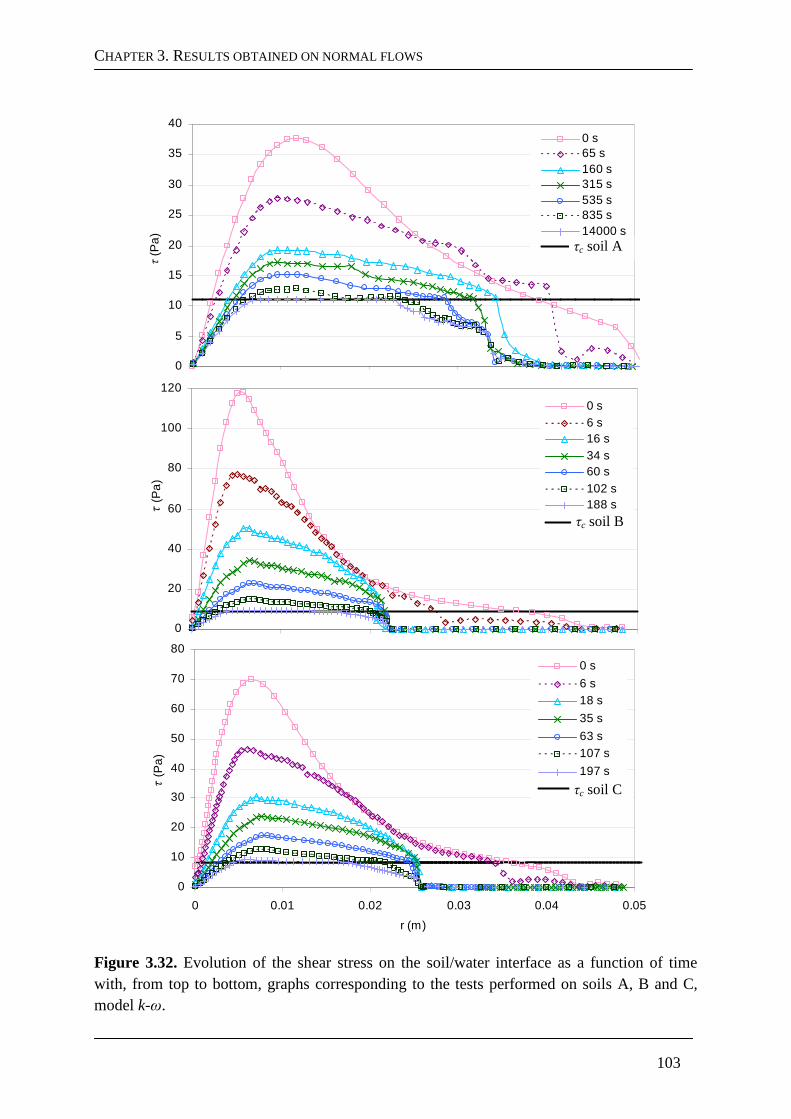
CHAPTER 3. RESULTS OBTAINED ON NORMAL FLOWS
103
0
5
10
15
20
25
30
35
40
τ (
Pa
)0 s65 s160 s315 s535 s835 s14000 stauc SC
0
20
40
60
80
100
120
τ (
Pa
)
0 s6 s16 s34 s60 s102 s188 stauc PR
0
10
20
30
40
50
60
70
80
0 0.01 0.02 0.03 0.04 0.05
r (m)
τ (
Pa
)
0 s
6 s18 s
35 s
63 s107 s
197 stauc KB
Figure 3.32. Evolution of the shear stress on the soil/water interface as a function of time with, from top to bottom, graphs corresponding to the tests performed on soils A, B and C, model k-ω.
τc soil A
τc soil B
τc soil C
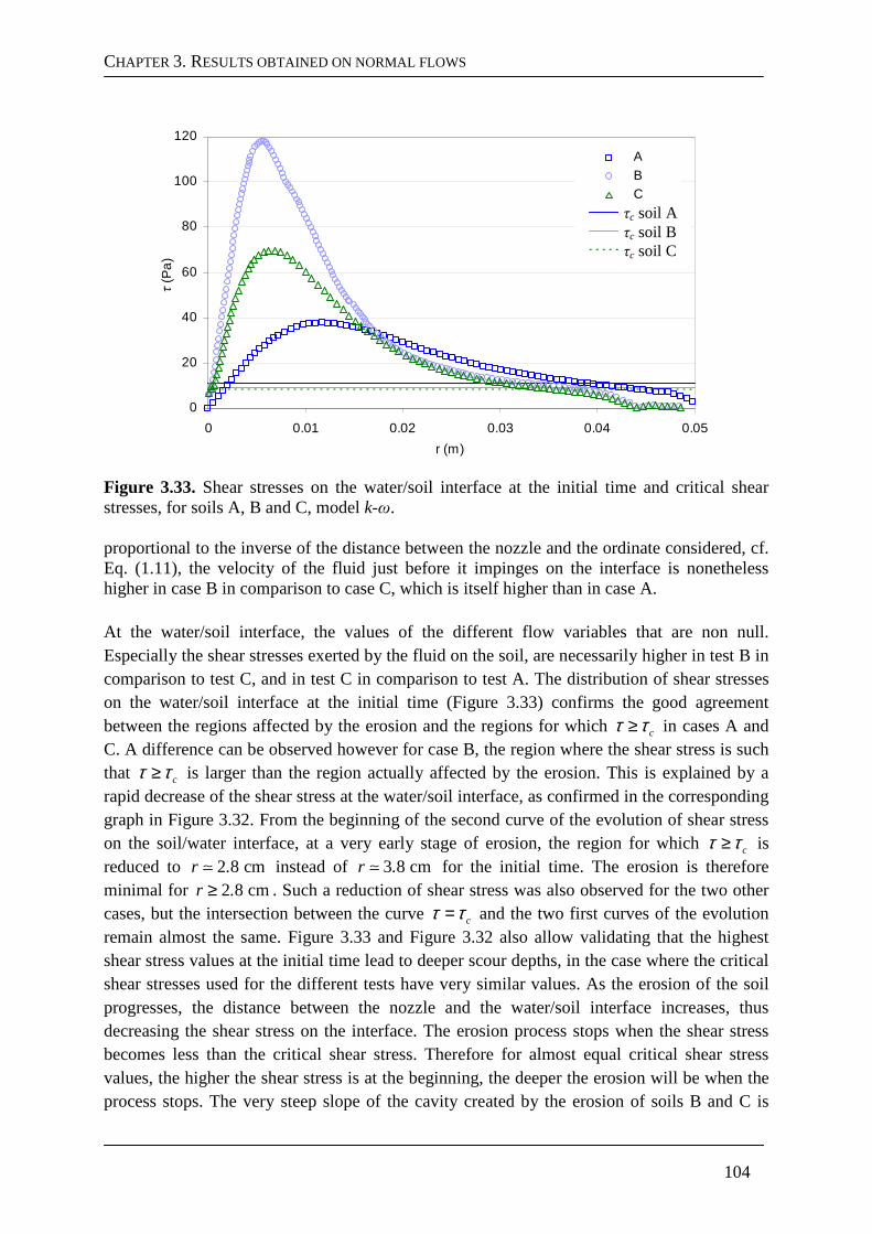
CHAPTER 3. RESULTS OBTAINED ON NORMAL FLOWS
104
0
20
40
60
80
100
120
0 0.01 0.02 0.03 0.04 0.05
r (m)
τ (
Pa
)AB CtaucAtaucBtaucC
Figure 3.33. Shear stresses on the water/soil interface at the initial time and critical shear stresses, for soils A, B and C, model k-ω. proportional to the inverse of the distance between the nozzle and the ordinate considered, cf. Eq. (1.11), the velocity of the fluid just before it impinges on the interface is nonetheless higher in case B in comparison to case C, which is itself higher than in case A. At the water/soil interface, the values of the different flow variables that are non null. Especially the shear stresses exerted by the fluid on the soil, are necessarily higher in test B in comparison to test C, and in test C in comparison to test A. The distribution of shear stresses on the water/soil interface at the initial time (Figure 3.33) confirms the good agreement between the regions affected by the erosion and the regions for which cτ τ≥ in cases A and C. A difference can be observed however for case B, the region where the shear stress is such that cτ τ≥ is larger than the region actually affected by the erosion. This is explained by a rapid decrease of the shear stress at the water/soil interface, as confirmed in the corresponding graph in Figure 3.32. From the beginning of the second curve of the evolution of shear stress on the soil/water interface, at a very early stage of erosion, the region for which cτ τ≥ is reduced to 2 8 cmr .≃ instead of 3 8 cmr .≃ for the initial time. The erosion is therefore minimal for 2 8 cmr .≥ . Such a reduction of shear stress was also observed for the two other cases, but the intersection between the curve cτ τ= and the two first curves of the evolution remain almost the same. Figure 3.33 and Figure 3.32 also allow validating that the highest shear stress values at the initial time lead to deeper scour depths, in the case where the critical shear stresses used for the different tests have very similar values. As the erosion of the soil progresses, the distance between the nozzle and the water/soil interface increases, thus decreasing the shear stress on the interface. The erosion process stops when the shear stress becomes less than the critical shear stress. Therefore for almost equal critical shear stress values, the higher the shear stress is at the beginning, the deeper the erosion will be when the process stops. The very steep slope of the cavity created by the erosion of soils B and C is
τc soil A τc soil B τc soil C
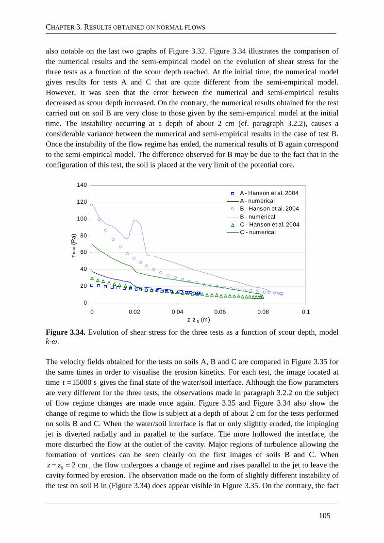
CHAPTER 3. RESULTS OBTAINED ON NORMAL FLOWS
105
also notable on the last two graphs of Figure 3.32. Figure 3.34 illustrates the comparison of the numerical results and the semi-empirical model on the evolution of shear stress for the three tests as a function of the scour depth reached. At the initial time, the numerical model gives results for tests A and C that are quite different from the semi-empirical model. However, it was seen that the error between the numerical and semi-empirical results decreased as scour depth increased. On the contrary, the numerical results obtained for the test carried out on soil B are very close to those given by the semi-empirical model at the initial time. The instability occurring at a depth of about 2 cm (cf. paragraph 3.2.2), causes a considerable variance between the numerical and semi-empirical results in the case of test B. Once the instability of the flow regime has ended, the numerical results of B again correspond to the semi-empirical model. The difference observed for B may be due to the fact that in the configuration of this test, the soil is placed at the very limit of the potential core.
0
20
40
60
80
100
120
140
0 0.02 0.04 0.06 0.08 0.1z-z 0 (m)
τm
ax (
Pa)
A - Hanson et al. 2004A - numericalB - Hanson et al. 2004B - numericalC - Hanson et al. 2004C - numerical
Figure 3.34. Evolution of shear stress for the three tests as a function of scour depth, model k-ω. The velocity fields obtained for the tests on soils A, B and C are compared in Figure 3.35 for the same times in order to visualise the erosion kinetics. For each test, the image located at time 15000 st = gives the final state of the water/soil interface. Although the flow parameters are very different for the three tests, the observations made in paragraph 3.2.2 on the subject of flow regime changes are made once again. Figure 3.35 and Figure 3.34 also show the change of regime to which the flow is subject at a depth of about 2 cm for the tests performed on soils B and C. When the water/soil interface is flat or only slightly eroded, the impinging jet is diverted radially and in parallel to the surface. The more hollowed the interface, the more disturbed the flow at the outlet of the cavity. Major regions of turbulence allowing the formation of vortices can be seen clearly on the first images of soils B and C. When
0 2 cmz z− ≃ , the flow undergoes a change of regime and rises parallel to the jet to leave the cavity formed by erosion. The observation made on the form of slightly different instability of the test on soil B in (Figure 3.34) does appear visible in Figure 3.35. On the contrary, the fact
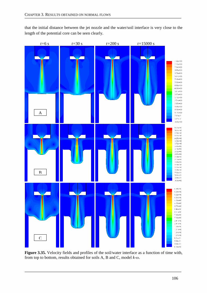
CHAPTER 3. RESULTS OBTAINED ON NORMAL FLOWS
106
that the initial distance between the jet nozzle and the water/soil interface is very close to the length of the potential core can be seen clearly.
t=6 s t=30 s t=200 s t=15000 s
Figure 3.35. Velocity fields and profiles of the soil/water interface as a function of time with, from top to bottom, results obtained for soils A, B and C, model k-ω.
A
B
C
CHAPTER 3. RESULTS OBTAINED ON NORMAL FLOWS
107
3.3.3. Discussion
The first element of discussion concerns the experimental validation of the change of flow regime as a function of cavity depth (cf. paragraph 3.2.3) observed with the numerical results of the k-ω model presented above. Whatever the test considered, the flow is strongly diverted at the end of the erosion process. Some studies carried out on the erosion of granular soils by jet flows propose determining the transition between SD and WD regimes. The formulations obtained all rely on the initial data of the test. From their experimental study [Moore and Masch 1962] deduced that the transition between the SD and WD regimes, between the different final shapes of cavities, depends only on the ratio 0 0z d . 0 0 7z d > the flow regime is SD, if not, for 0 0 7z d < the flow is WD. On the other hand, [Hollick 1976] showed that even in the case of a constant ratio 0 0z d , the two flow regimes can be observed. According to [Aderibigbe and Rajaratnam 1996], the transition between these two flow regimes is a function of the Froude number associated with the relative diameter of the grains ( 0Fr ) and the ratio 0 0z d , with
( )0 0 wFr U gD ρ ρ= ∆ . If ( )0 0 0 0.35Fr z d > , the flow at the end of the erosion process is SD. For the tests performed on soils A, B and C, the ratios 0 0z d are 23.0, 6.4 and 12.3, respectively. However, all the cavities obtained at the end of the erosion process, experimentally (except perhaps for soil B) and numerically present narrow and deep erosion scours. These results agree with the deductions of [Hollick 1976] on the non correspondence of ratio 0 0 7z d > and the flow regime. The diameter of the grains is difficult to determine for a cohesive soil, and even more so for a mixture of soil and cement (sol B). The determination of 0Fr , as defined here, is therefore not pertinent for these erosion tests. For the three models, as different as they are, the change of flow regime always occurs at a depth close to two centimetres. Additional numerical and experimental research on this subject would undoubtedly result in the development of a new law making it possible to predict the flow regime during the erosion process as a function of the soil erosion parameters, dk and τc , of 0U and the ratio 0 0z d . The second element of discussion concerns the pertinence of the numerical results and the pertinence of the JET interpretation model. Given the results of these different models, it is clear that the k-ω turbulence model is that which best models the Jet Erosion Tests. In addition to the elements of validation set out in paragraph 3.2.3, above all regarding the non existence of the SD regimes even in narrow deep cavities, this model made it possible to predict the evolution of the water/soil interface with considerable precision. Although less precision is obtained for the simulations performed with the k-ε model, the results are nonetheless of the same order of magnitude as the experimental and semi-empirical results. The differences observed are of the same order of magnitude as the uncertainties usually found in soil mechanics for geotechnical parameters. The correspondence of the numerical, semi-empirical and experimental results, at least in terms of order of magnitude, is fully validated for these three models. This validation of the numerical modelling method and of the JET interpretation model of [Hanson and Cook 2004] is important. It is now possible to model the erosion of a cohesive soil by a turbulent flow with simplified models and reasonable calculation times. Another result is that we can consider that the interpretation
CHAPTER 3. RESULTS OBTAINED ON NORMAL FLOWS
108
model of the Jet Erosion Test is pertinent in spite of its simplicity. The erosion parameters found with the JET with the erosion law (1.1) used to obtain the evolution of the water/soil interface as a function of time are validated after performing a complex and mechanically based CFD numerical modelling. However, the physical meaning of the erosion parameters remains to be determined. It is also necessary to bear in mind that the erosion law (1.1) was imposed. The implementation of another erosion law with erosion parameters permitting the conservation of the cΓ would perhaps allow obtaining numerical results in good agreement with the experimental results, cf. Chapter 5. Also, determining ranges of erosion parameters for which the interpretation model is valid requires building additional models. The ranges of erosion parameters covered by these three models are about 510− to 6 210 m .s/kg− for the dk and from 8 to 11 Pa for the cτ . Carrying out a complementary study on this subject falls within the perspectives of this PhD thesis.
3.4. Conclusions on the application to jet flows
This chapter concerns the application of the numerical model to jet flows. We first focus on the validation of the numerical model without erosion. The independence of the results from mesh density was verified and the influence of the turbulence models was studied. Three turbulence models were considered: the ε−k , ω−k and RSM models. Globally, the results of the RSM model were closest to the empirical formulations found in the literature. The
ε−k model was in good agreement with the results in the literature for the shear stress on the wall. The ω−k model was in good agreement with the velocity fields and the pressure in the flow. Secondly, the numerical model with erosion was applied to a JET. The results are compared in-depth to the interpretation model of [Hanson et al. 2004]. The difficulties of convergence of the RSM do not permit modelling the full erosion process. The results given by the ω−k model were in good agreement with the semi-empirical and experimental results. The results given by the ε−k model corresponded less well but remained in the same order of magnitude. Furthermore, major phenomena of recirculation and changes of flow regime according to depth were observed with the ω−k model. The study of the sensitivity of the numerical model to the erosion parameters was then described. It showed that a very narrow range of parameters makes it possible to obtain numerical results in good agreement with the semi-empirical and experimental results. A discussion was proposed on the measurement methods of the results in the literature. Apparently, they are reliable and completely independent, although the error margin of the results proposed was not given. The changes of regime observed after a certain scour depth in the case of the ω−k model were also the subject of the discussion. Several experimental validations on the observation of the SD and WD flow regimes were found in the literature. In conclusion, we deduced that this study is an important element for validating the interpretation model of [Hanson and Cook 2004] and the numerical modelling method, at least in terms of magnitude.
CHAPTER 3. RESULTS OBTAINED ON NORMAL FLOWS
109
Thirdly, two other JETs were modelled. The characteristics of different soils were described. The range of erosion parameters covered by these tests, although rather narrow, is fairly representative of the tests that are likely to be carried out on French embankment dams and dikes. However, the magnitude of the hydraulic parameters involved is considerable. The results obtained for the modelling performed with the ω−k are in good agreement with the experimental results and the semi-empirical model. The results obtained with the ε−k model are of the same order of magnitude. The comparison of the different flow characteristics and the shape of erosion figures was performed between the three tests. Then a discussion was proposed on the transition between the SD and WD flow regimes. Deepening this numerical study would undoubtedly lead to the development of a new law making it possible to predict this transition. In addition, the pertinence of the JET interpretation model was discussed with the result that important elements of validation were added to the interpretation method developed by [Hanson and Cook 2004]. Using only the flow and erosion parameters, it was possible in three different cases to obtain, numerically, the evolution of scour depth as a function of time with a precision to within 30% relative error. We deduced that the JET interpretation model was validated, at least in terms of order of magnitude and for the range of erosion parameters modelled. Nonetheless, no element allowed us to conclude on the physical meaning of the erosion parameters obtained. Major elements of validation of the Jet Erosion Test interpretation model and the numerical model were provided in this chapter. The applications presented here were the subject of three publications. [Mercier et al. 2012] is a conference article with proceedings, that sets out the model of the test performed on soil A. The numerical, experimental and semi-empirical results of [Hanson and Cook 2004] are compared. [Mercier et al. submitted] focuses on the modelling method and the validation of its pertinence. The results are compared only with the semi-empirical model. [Mercier et al. submitted-b] described the modelling of three JETs and compared the numerical results with the experimental ones and with those of the semi-empirical model. This article also presents the elements used to validate the JET interpretation model. In the following chapter, additional elements for validating the numerical model are considered. A radically different flow configuration is adopted. In Chapter 4 attention will be given to tangential flows at the water/soil interface. A plane Poiseuille flow configuration is tested and a detailed description of the flow in a Hole Erosion Test device is given. Chapter 4 also describes theoretical, analytical and experimental elements of the numerical model.

CHAPTER 3. RESULTS OBTAINED ON NORMAL FLOWS
110
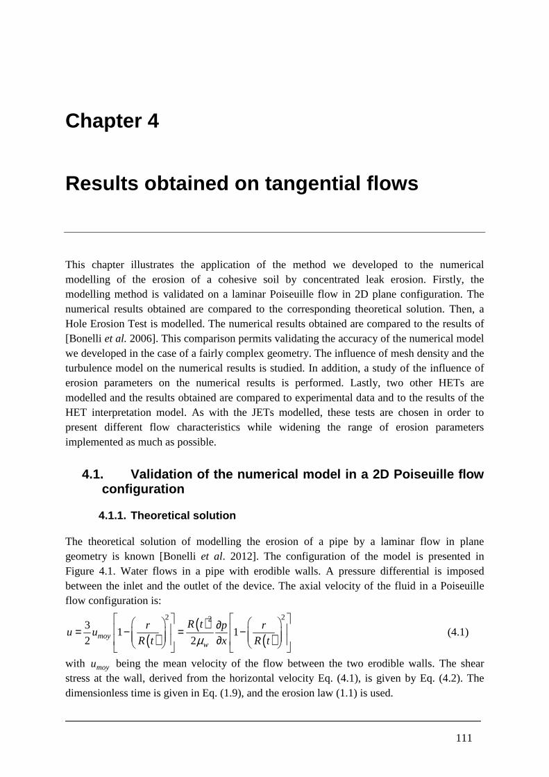
111
Chapter 4
Results obtained on tangential flows
This chapter illustrates the application of the method we developed to the numerical modelling of the erosion of a cohesive soil by concentrated leak erosion. Firstly, the modelling method is validated on a laminar Poiseuille flow in 2D plane configuration. The numerical results obtained are compared to the corresponding theoretical solution. Then, a Hole Erosion Test is modelled. The numerical results obtained are compared to the results of [Bonelli et al. 2006]. This comparison permits validating the accuracy of the numerical model we developed in the case of a fairly complex geometry. The influence of mesh density and the turbulence model on the numerical results is studied. In addition, a study of the influence of erosion parameters on the numerical results is performed. Lastly, two other HETs are modelled and the results obtained are compared to experimental data and to the results of the HET interpretation model. As with the JETs modelled, these tests are chosen in order to present different flow characteristics while widening the range of erosion parameters implemented as much as possible.
4.1. Validation of the numerical model in a 2D Pois euille flow configuration
4.1.1. Theoretical solution
The theoretical solution of modelling the erosion of a pipe by a laminar flow in plane geometry is known [Bonelli et al. 2012]. The configuration of the model is presented in Figure 4.1. Water flows in a pipe with erodible walls. A pressure differential is imposed between the inlet and the outlet of the device. The axial velocity of the fluid in a Poiseuille flow configuration is:
( )( )
( )
2 223
1 12 2moy
w
R tr p ru u
R t x R t
∂ = − = − ∂ µ
(4.1)
with moyu being the mean velocity of the flow between the two erodible walls. The shear stress at the wall, derived from the horizontal velocity Eq. (4.1), is given by Eq. (4.2). The dimensionless time is given in Eq. (1.9), and the erosion law (1.1) is used.
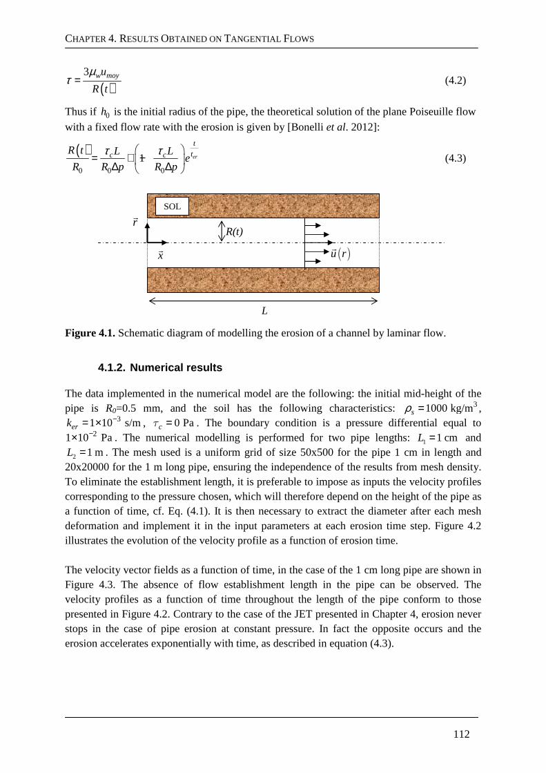
CHAPTER 4. RESULTS OBTAINED ON TANGENTIAL FLOWS
112
( )3 w moyu
R t=
µτ (4.2)
Thus if 0h is the initial radius of the pipe, the theoretical solution of the plane Poiseuille flow
with a fixed flow rate with the erosion is given by [Bonelli et al. 2012]:
( )0 0 0
1 er
t
tc cR t L Le
R R p R p
= + − ∆ ∆
τ τ (4.3)
Figure 4.1. Schematic diagram of modelling the erosion of a channel by laminar flow.
4.1.2. Numerical results
The data implemented in the numerical model are the following: the initial mid-height of the pipe is R0=0.5 mm, and the soil has the following characteristics: 31000 kg/msρ = ,
31 10 s/merk −= × , 0 Paτc = . The boundary condition is a pressure differential equal to 21 10 Pa−× . The numerical modelling is performed for two pipe lengths: 1 1 cmL = and
2 1 mL = . The mesh used is a uniform grid of size 50x500 for the pipe 1 cm in length and 20x20000 for the 1 m long pipe, ensuring the independence of the results from mesh density. To eliminate the establishment length, it is preferable to impose as inputs the velocity profiles corresponding to the pressure chosen, which will therefore depend on the height of the pipe as a function of time, cf. Eq. (4.1). It is then necessary to extract the diameter after each mesh deformation and implement it in the input parameters at each erosion time step. Figure 4.2 illustrates the evolution of the velocity profile as a function of erosion time. The velocity vector fields as a function of time, in the case of the 1 cm long pipe are shown in Figure 4.3. The absence of flow establishment length in the pipe can be observed. The velocity profiles as a function of time throughout the length of the pipe conform to those presented in Figure 4.2. Contrary to the case of the JET presented in Chapter 4, erosion never stops in the case of pipe erosion at constant pressure. In fact the opposite occurs and the erosion accelerates exponentially with time, as described in equation (4.3).
R(t)
L
( )u r
x
r
SOL
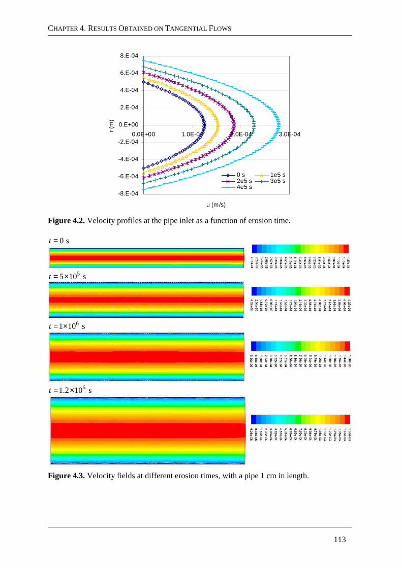
CHAPTER 4. RESULTS OBTAINED ON TANGENTIAL FLOWS
113
-8.E-04
-6.E-04
-4.E-04
-2.E-04
0.E+00
2.E-04
4.E-04
6.E-04
8.E-04
0.0E+00 1.0E-04 2.0E-04 3.0E-04
u (m/s)
r (m
)
0 s 1e5 s2e5 s 3e5 s4e5 s
Figure 4.2. Velocity profiles at the pipe inlet as a function of erosion time.
0 st =
55 10 st = ×
61 10 st = ×
61.2 10 st = ×
Figure 4.3. Velocity fields at different erosion times, with a pipe 1 cm in length.
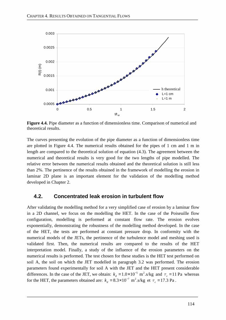
CHAPTER 4. RESULTS OBTAINED ON TANGENTIAL FLOWS
114
0.0005
0.001
0.0015
0.002
0.0025
0.003
0 0.5 1 1.5 2t/t er
R(t
) (m
)
h théoriqueL=1 cmL=1 m
Figure 4.4. Pipe diameter as a function of dimensionless time. Comparison of numerical and theoretical results.
The curves presenting the evolution of the pipe diameter as a function of dimensionless time are plotted in Figure 4.4. The numerical results obtained for the pipes of 1 cm and 1 m in length are compared to the theoretical solution of equation (4.3). The agreement between the numerical and theoretical results is very good for the two lengths of pipe modelled. The relative error between the numerical results obtained and the theoretical solution is still less than 2%. The pertinence of the results obtained in the framework of modelling the erosion in laminar 2D plane is an important element for the validation of the modelling method developed in Chapter 2.
4.2. Concentrated leak erosion in turbulent flow
After validating the modelling method for a very simplified case of erosion by a laminar flow in a 2D channel, we focus on the modelling the HET. In the case of the Poiseuille flow configuration, modelling is performed at constant flow rate. The erosion evolves exponentially, demonstrating the robustness of the modelling method developed. In the case of the HET, the tests are performed at constant pressure drop. In conformity with the numerical models of the JETs, the pertinence of the turbulence model and meshing used is validated first. Then, the numerical results are compared to the results of the HET interpretation model. Finally, a study of the influence of the erosion parameters on the numerical results is performed. The test chosen for these studies is the HET test performed on soil A, the soil on which the JET modelled in paragraph 3.2 was performed. The erosion parameters found experimentally for soil A with the JET and the HET present considerable differences. In the case of the JET, we obtain: 5 21.0 10 m .s/kgdk −= × and 11 Pacτ = whereas for the HET, the parameters obtained are: 7 28.3 10 m .s/kgdk −= × et 17.3 Pacτ = .
h theoretical
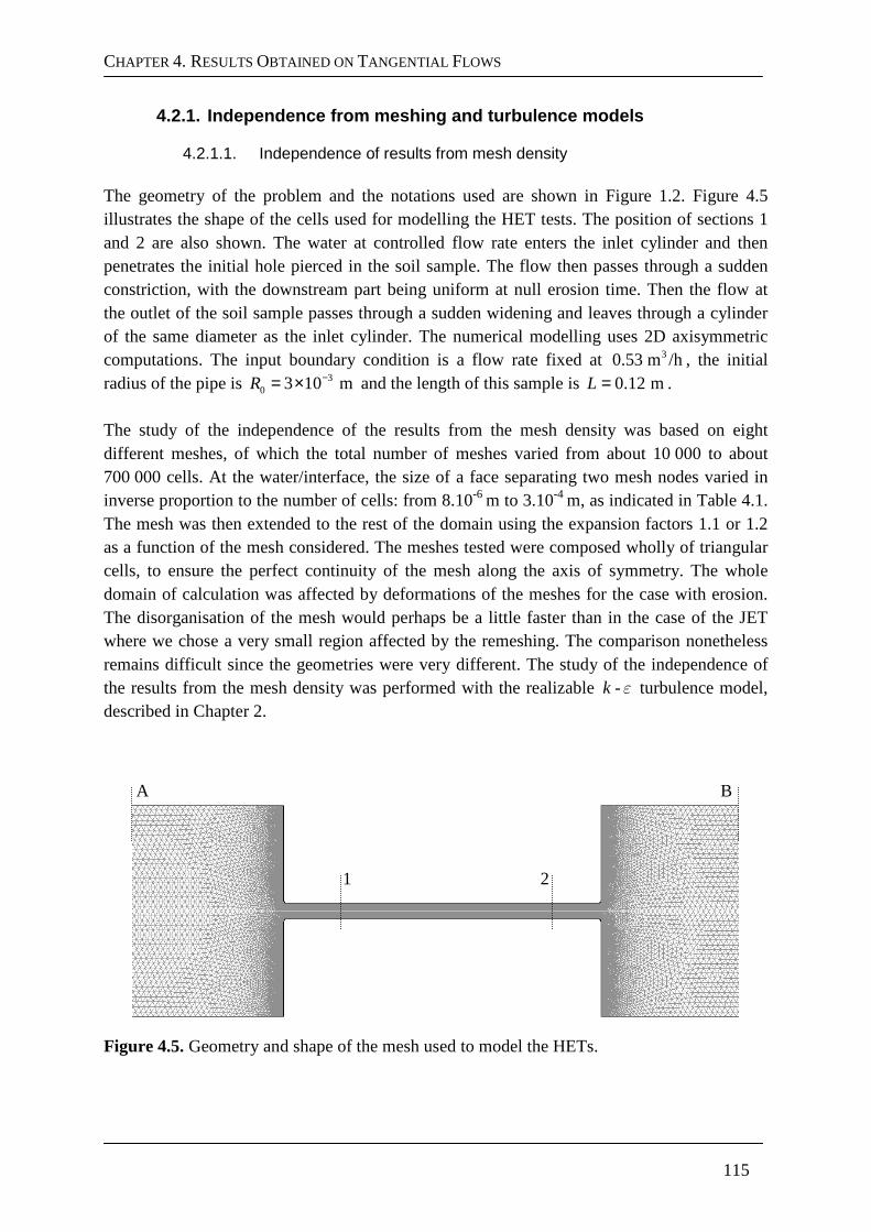
CHAPTER 4. RESULTS OBTAINED ON TANGENTIAL FLOWS
115
4.2.1. Independence from meshing and turbulence mod els
4.2.1.1. Independence of results from mesh density The geometry of the problem and the notations used are shown in Figure 1.2. Figure 4.5 illustrates the shape of the cells used for modelling the HET tests. The position of sections 1 and 2 are also shown. The water at controlled flow rate enters the inlet cylinder and then penetrates the initial hole pierced in the soil sample. The flow then passes through a sudden constriction, with the downstream part being uniform at null erosion time. Then the flow at the outlet of the soil sample passes through a sudden widening and leaves through a cylinder of the same diameter as the inlet cylinder. The numerical modelling uses 2D axisymmetric computations. The input boundary condition is a flow rate fixed at 30.53 m /h, the initial radius of the pipe is 3
0 3 10 mR −= × and the length of this sample is 0.12 mL = . The study of the independence of the results from the mesh density was based on eight different meshes, of which the total number of meshes varied from about 10 000 to about 700 000 cells. At the water/interface, the size of a face separating two mesh nodes varied in inverse proportion to the number of cells: from 8.10-6 m to 3.10-4 m, as indicated in Table 4.1. The mesh was then extended to the rest of the domain using the expansion factors 1.1 or 1.2 as a function of the mesh considered. The meshes tested were composed wholly of triangular cells, to ensure the perfect continuity of the mesh along the axis of symmetry. The whole domain of calculation was affected by deformations of the meshes for the case with erosion. The disorganisation of the mesh would perhaps be a little faster than in the case of the JET where we chose a very small region affected by the remeshing. The comparison nonetheless remains difficult since the geometries were very different. The study of the independence of the results from the mesh density was performed with the realizable k - ε turbulence model, described in Chapter 2.
Figure 4.5. Geometry and shape of the mesh used to model the HETs.
1 2
A B
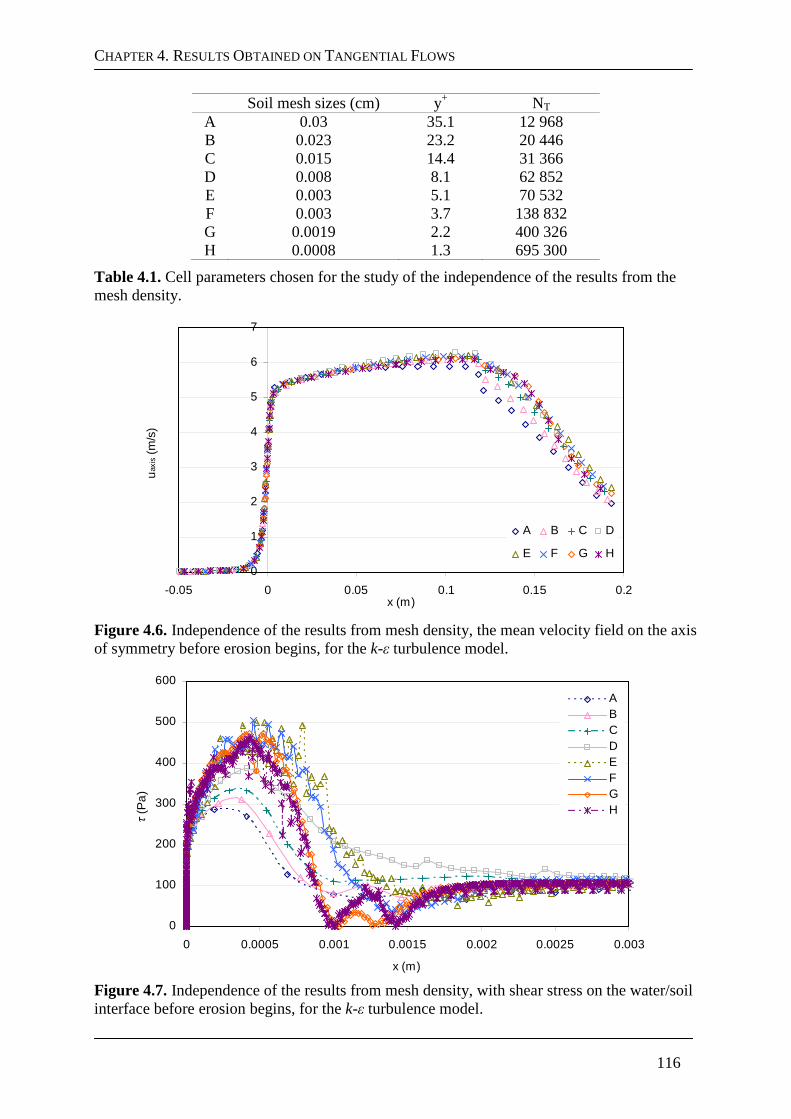
CHAPTER 4. RESULTS OBTAINED ON TANGENTIAL FLOWS
116
Soil mesh sizes (cm) y+ NT A 0.03 35.1 12 968 B 0.023 23.2 20 446 C 0.015 14.4 31 366 D 0.008 8.1 62 852 E 0.003 5.1 70 532 F 0.003 3.7 138 832 G 0.0019 2.2 400 326 H 0.0008 1.3 695 300
Table 4.1. Cell parameters chosen for the study of the independence of the results from the mesh density.
0
1
2
3
4
5
6
7
-0.05 0 0.05 0.1 0.15 0.2x (m)
uax
is (
m/s
)
A B C D
E F G H
Figure 4.6. Independence of the results from mesh density, the mean velocity field on the axis of symmetry before erosion begins, for the k-ε turbulence model.
0
100
200
300
400
500
600
0 0.0005 0.001 0.0015 0.002 0.0025 0.003
x (m)
τ (P
a)
ABCDEFGH
Figure 4.7. Independence of the results from mesh density, with shear stress on the water/soil interface before erosion begins, for the k-ε turbulence model.
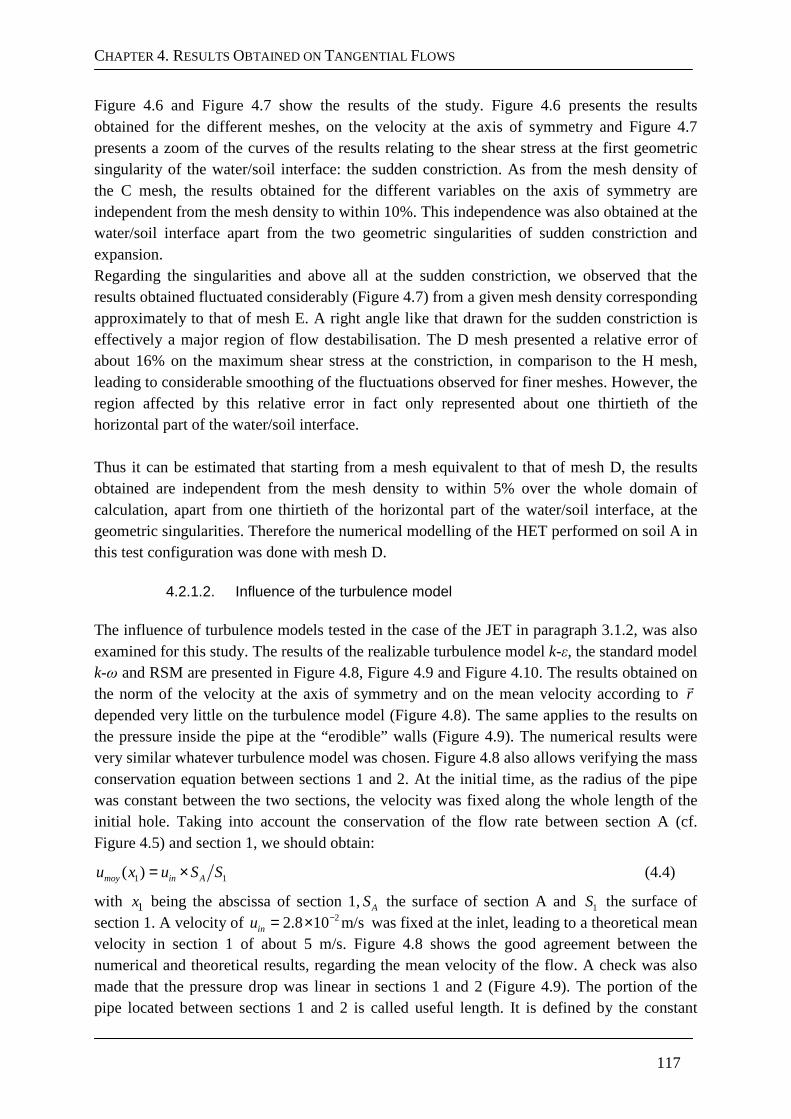
CHAPTER 4. RESULTS OBTAINED ON TANGENTIAL FLOWS
117
Figure 4.6 and Figure 4.7 show the results of the study. Figure 4.6 presents the results obtained for the different meshes, on the velocity at the axis of symmetry and Figure 4.7 presents a zoom of the curves of the results relating to the shear stress at the first geometric singularity of the water/soil interface: the sudden constriction. As from the mesh density of the C mesh, the results obtained for the different variables on the axis of symmetry are independent from the mesh density to within 10%. This independence was also obtained at the water/soil interface apart from the two geometric singularities of sudden constriction and expansion. Regarding the singularities and above all at the sudden constriction, we observed that the results obtained fluctuated considerably (Figure 4.7) from a given mesh density corresponding approximately to that of mesh E. A right angle like that drawn for the sudden constriction is effectively a major region of flow destabilisation. The D mesh presented a relative error of about 16% on the maximum shear stress at the constriction, in comparison to the H mesh, leading to considerable smoothing of the fluctuations observed for finer meshes. However, the region affected by this relative error in fact only represented about one thirtieth of the horizontal part of the water/soil interface. Thus it can be estimated that starting from a mesh equivalent to that of mesh D, the results obtained are independent from the mesh density to within 5% over the whole domain of calculation, apart from one thirtieth of the horizontal part of the water/soil interface, at the geometric singularities. Therefore the numerical modelling of the HET performed on soil A in this test configuration was done with mesh D.
4.2.1.2. Influence of the turbulence model The influence of turbulence models tested in the case of the JET in paragraph 3.1.2, was also examined for this study. The results of the realizable turbulence model k-ε, the standard model k-ω and RSM are presented in Figure 4.8, Figure 4.9 and Figure 4.10. The results obtained on the norm of the velocity at the axis of symmetry and on the mean velocity according to r
depended very little on the turbulence model (Figure 4.8). The same applies to the results on the pressure inside the pipe at the “erodible” walls (Figure 4.9). The numerical results were very similar whatever turbulence model was chosen. Figure 4.8 also allows verifying the mass conservation equation between sections 1 and 2. At the initial time, as the radius of the pipe was constant between the two sections, the velocity was fixed along the whole length of the initial hole. Taking into account the conservation of the flow rate between section A (cf. Figure 4.5) and section 1, we should obtain:
1 1( )moy in Au x u S S= × (4.4)
with 1x being the abscissa of section 1,AS the surface of section A and 1S the surface of section 1. A velocity of 22.8 10 m/sinu −= × was fixed at the inlet, leading to a theoretical mean velocity in section 1 of about 5 m/s. Figure 4.8 shows the good agreement between the numerical and theoretical results, regarding the mean velocity of the flow. A check was also made that the pressure drop was linear in sections 1 and 2 (Figure 4.9). The portion of the pipe located between sections 1 and 2 is called useful length. It is defined by the constant
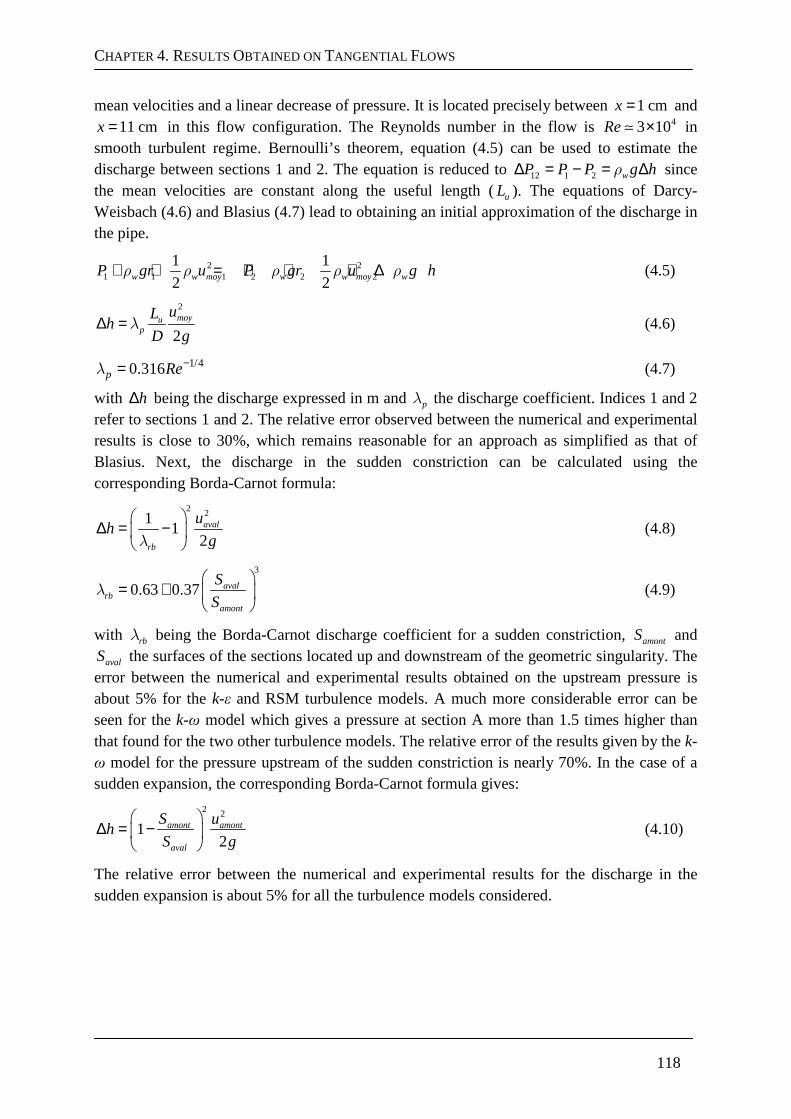
CHAPTER 4. RESULTS OBTAINED ON TANGENTIAL FLOWS
118
mean velocities and a linear decrease of pressure. It is located precisely between 1 cmx = and 11 cmx = in this flow configuration. The Reynolds number in the flow is 43 10Re ×≃ in
smooth turbulent regime. Bernoulli’s theorem, equation (4.5) can be used to estimate the discharge between sections 1 and 2. The equation is reduced to 12 1 2 wP P P g hρ∆ = − = ∆ since the mean velocities are constant along the useful length ( uL ). The equations of Darcy-Weisbach (4.6) and Blasius (4.7) lead to obtaining an initial approximation of the discharge in the pipe.
2 21 1 1 2 2 2
1 1
2 2w w moy w w moy wP gr u P gr u g hρ ρ ρ ρ ρ+ + = + + + ∆ (4.5)
2
2moyu
p
uLh
D gλ∆ = (4.6)
1/40.316p Reλ −= (4.7)
with h∆ being the discharge expressed in m and pλ the discharge coefficient. Indices 1 and 2 refer to sections 1 and 2. The relative error observed between the numerical and experimental results is close to 30%, which remains reasonable for an approach as simplified as that of Blasius. Next, the discharge in the sudden constriction can be calculated using the corresponding Borda-Carnot formula:
2 211
2aval
rb
uh
gλ
∆ = −
(4.8)
3
0.63 0.37 avalrb
amont
S
Sλ
= +
(4.9)
with rbλ being the Borda-Carnot discharge coefficient for a sudden constriction, amontS and
avalS the surfaces of the sections located up and downstream of the geometric singularity. The error between the numerical and experimental results obtained on the upstream pressure is about 5% for the k-ε and RSM turbulence models. A much more considerable error can be seen for the k-ω model which gives a pressure at section A more than 1.5 times higher than that found for the two other turbulence models. The relative error of the results given by the k-ω model for the pressure upstream of the sudden constriction is nearly 70%. In the case of a sudden expansion, the corresponding Borda-Carnot formula gives:
2 2
12
amont amont
aval
S uh
S g
∆ = −
(4.10)
The relative error between the numerical and experimental results for the discharge in the sudden expansion is about 5% for all the turbulence models considered.
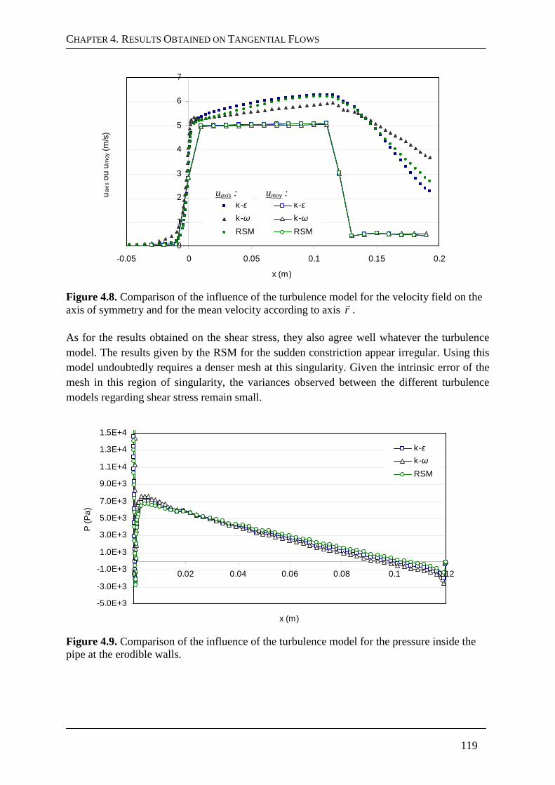
CHAPTER 4. RESULTS OBTAINED ON TANGENTIAL FLOWS
119
0
1
2
3
4
5
6
7
-0.05 0 0.05 0.1 0.15 0.2
x (m)
uax
is o
u u
moy
(m/s
)
k-ε k-ε
k-ω k-ω
RSM RSM
Figure 4.8. Comparison of the influence of the turbulence model for the velocity field on the axis of symmetry and for the mean velocity according to axis r
.
As for the results obtained on the shear stress, they also agree well whatever the turbulence model. The results given by the RSM for the sudden constriction appear irregular. Using this model undoubtedly requires a denser mesh at this singularity. Given the intrinsic error of the mesh in this region of singularity, the variances observed between the different turbulence models regarding shear stress remain small.
-5.0E+3
-3.0E+3
-1.0E+3
1.0E+3
3.0E+3
5.0E+3
7.0E+3
9.0E+3
1.1E+4
1.3E+4
1.5E+4
0 0.02 0.04 0.06 0.08 0.1 0.12
x (m)
P (
Pa
)
k-ε
k-ω
RSM
Figure 4.9. Comparison of the influence of the turbulence model for the pressure inside the pipe at the erodible walls.
uaxis : umoy :
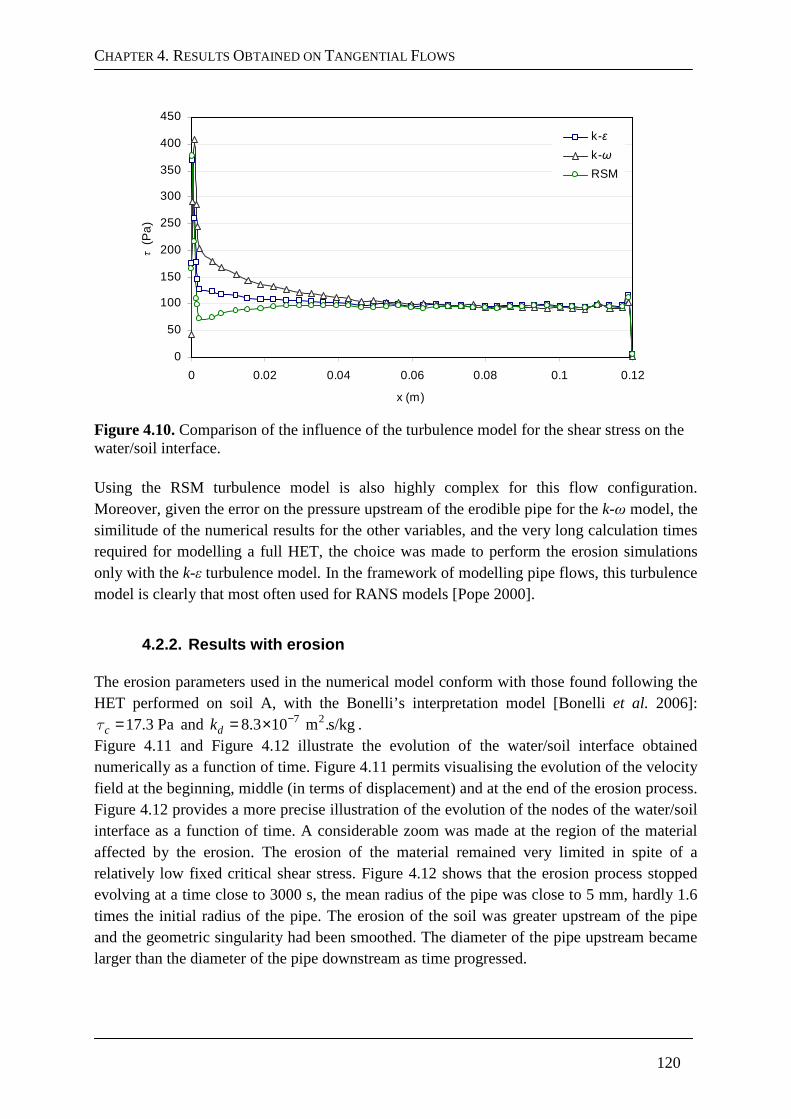
CHAPTER 4. RESULTS OBTAINED ON TANGENTIAL FLOWS
120
0
50
100
150
200
250
300
350
400
450
0 0.02 0.04 0.06 0.08 0.1 0.12
x (m)
τ (
Pa
)k-ε
k-ω
RSM
Figure 4.10. Comparison of the influence of the turbulence model for the shear stress on the water/soil interface. Using the RSM turbulence model is also highly complex for this flow configuration. Moreover, given the error on the pressure upstream of the erodible pipe for the k-ω model, the similitude of the numerical results for the other variables, and the very long calculation times required for modelling a full HET, the choice was made to perform the erosion simulations only with the k-ε turbulence model. In the framework of modelling pipe flows, this turbulence model is clearly that most often used for RANS models [Pope 2000].
4.2.2. Results with erosion
The erosion parameters used in the numerical model conform with those found following the HET performed on soil A, with the Bonelli’s interpretation model [Bonelli et al. 2006]:
17.3 Pacτ = and 7 28.3 10 m .s/kgdk −= × . Figure 4.11 and Figure 4.12 illustrate the evolution of the water/soil interface obtained numerically as a function of time. Figure 4.11 permits visualising the evolution of the velocity field at the beginning, middle (in terms of displacement) and at the end of the erosion process. Figure 4.12 provides a more precise illustration of the evolution of the nodes of the water/soil interface as a function of time. A considerable zoom was made at the region of the material affected by the erosion. The erosion of the material remained very limited in spite of a relatively low fixed critical shear stress. Figure 4.12 shows that the erosion process stopped evolving at a time close to 3000 s, the mean radius of the pipe was close to 5 mm, hardly 1.6 times the initial radius of the pipe. The erosion of the soil was greater upstream of the pipe and the geometric singularity had been smoothed. The diameter of the pipe upstream became larger than the diameter of the pipe downstream as time progressed.
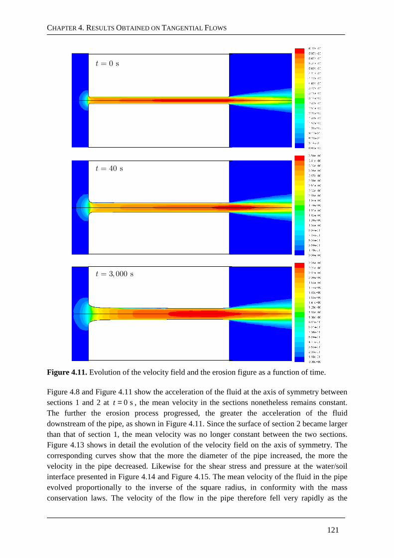
CHAPTER 4. RESULTS OBTAINED ON TANGENTIAL FLOWS
121
Figure 4.11. Evolution of the velocity field and the erosion figure as a function of time. Figure 4.8 and Figure 4.11 show the acceleration of the fluid at the axis of symmetry between sections 1 and 2 at 0 st = , the mean velocity in the sections nonetheless remains constant. The further the erosion process progressed, the greater the acceleration of the fluid downstream of the pipe, as shown in Figure 4.11. Since the surface of section 2 became larger than that of section 1, the mean velocity was no longer constant between the two sections. Figure 4.13 shows in detail the evolution of the velocity field on the axis of symmetry. The corresponding curves show that the more the diameter of the pipe increased, the more the velocity in the pipe decreased. Likewise for the shear stress and pressure at the water/soil interface presented in Figure 4.14 and Figure 4.15. The mean velocity of the fluid in the pipe evolved proportionally to the inverse of the square radius, in conformity with the mass conservation laws. The velocity of the flow in the pipe therefore fell very rapidly as the
0 st =
40 st =
3, 000 st =

CHAPTER 4. RESULTS OBTAINED ON TANGENTIAL FLOWS
122
diameter of the pipe increased. This explains that the shear stress exerted by the fluid on the soil also fell very rapidly as the diameter of the pipe increased. The shear stress rapidly became lower than the critical shear stress and the erosion process stopped after having progressed little. A considerable shear stress peak can be seen at the sudden constriction (cf. Figure 4.14). That is why the erosion is more considerable at the upstream geometrical singularity than in the rest of the pipe. The shear stress peak falls as the erosion process progresses.
0.003
0.0035
0.004
0.0045
0.005
0.0055
0.006
0.0065
0.007
0.0075
0.008
0 0.02 0.04 0.06 0.08 0.1 0.12
x (m)
r (m
)
0 s7 s22 s41 s69 s207 s546 s3310 s
Figure 4.12. Evolution of the profile of the water/soil interface as a function of time.
0
1
2
3
4
5
6
7
-0.05 0 0.05 0.1 0.15 0.2 0.25
x (m)
uax
is (
m/s
)
0 s7 s22 s41 s69 s207 s546 s3310 s
Figure 4.13. Evolution of the velocity field on the axis of symmetry as a function of time.
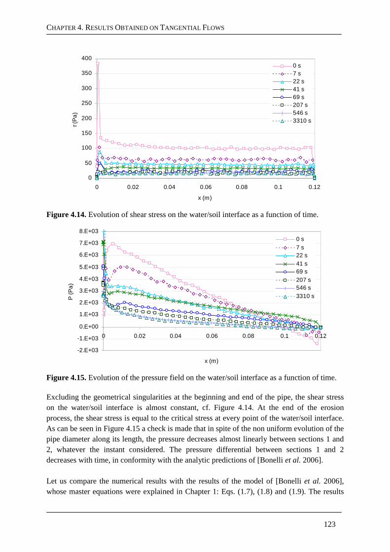
CHAPTER 4. RESULTS OBTAINED ON TANGENTIAL FLOWS
123
0
50
100
150
200
250
300
350
400
0 0.02 0.04 0.06 0.08 0.1 0.12
x (m)
τ (P
a)
0 s7 s22 s 41 s69 s207 s546 s3310 s
Figure 4.14. Evolution of shear stress on the water/soil interface as a function of time.
-2.E+03
-1.E+03
0.E+00
1.E+03
2.E+03
3.E+03
4.E+03
5.E+03
6.E+03
7.E+03
8.E+03
0 0.02 0.04 0.06 0.08 0.1 0.12
x (m)
P (
Pa
)
0 s7 s22 s41 s69 s207 s546 s3310 s
Figure 4.15. Evolution of the pressure field on the water/soil interface as a function of time.
Excluding the geometrical singularities at the beginning and end of the pipe, the shear stress on the water/soil interface is almost constant, cf. Figure 4.14. At the end of the erosion process, the shear stress is equal to the critical stress at every point of the water/soil interface. As can be seen in Figure 4.15 a check is made that in spite of the non uniform evolution of the pipe diameter along its length, the pressure decreases almost linearly between sections 1 and 2, whatever the instant considered. The pressure differential between sections 1 and 2 decreases with time, in conformity with the analytic predictions of [Bonelli et al. 2006]. Let us compare the numerical results with the results of the model of [Bonelli et al. 2006], whose master equations were explained in Chapter 1: Eqs. (1.7), (1.8) and (1.9). The results
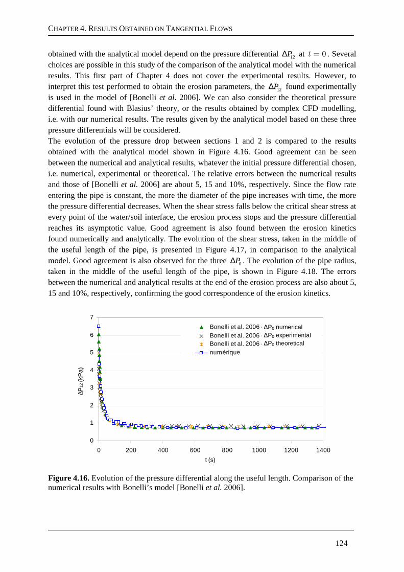
CHAPTER 4. RESULTS OBTAINED ON TANGENTIAL FLOWS
124
obtained with the analytical model depend on the pressure differential 12P∆ at 0t = . Several choices are possible in this study of the comparison of the analytical model with the numerical results. This first part of Chapter 4 does not cover the experimental results. However, to interpret this test performed to obtain the erosion parameters, the 12P∆ found experimentally is used in the model of [Bonelli et al. 2006]. We can also consider the theoretical pressure differential found with Blasius’ theory, or the results obtained by complex CFD modelling, i.e. with our numerical results. The results given by the analytical model based on these three pressure differentials will be considered. The evolution of the pressure drop between sections 1 and 2 is compared to the results obtained with the analytical model shown in Figure 4.16. Good agreement can be seen between the numerical and analytical results, whatever the initial pressure differential chosen, i.e. numerical, experimental or theoretical. The relative errors between the numerical results and those of [Bonelli et al. 2006] are about 5, 15 and 10%, respectively. Since the flow rate entering the pipe is constant, the more the diameter of the pipe increases with time, the more the pressure differential decreases. When the shear stress falls below the critical shear stress at every point of the water/soil interface, the erosion process stops and the pressure differential reaches its asymptotic value. Good agreement is also found between the erosion kinetics found numerically and analytically. The evolution of the shear stress, taken in the middle of the useful length of the pipe, is presented in Figure 4.17, in comparison to the analytical model. Good agreement is also observed for the three 0P∆ . The evolution of the pipe radius, taken in the middle of the useful length of the pipe, is shown in Figure 4.18. The errors between the numerical and analytical results at the end of the erosion process are also about 5, 15 and 10%, respectively, confirming the good correspondence of the erosion kinetics.
0
1
2
3
4
5
6
7
0 200 400 600 800 1000 1200 1400
t (s)
∆P
12 (
kPa)
Bonelli et al. 2006 - ∆PnumériqueBonelli et al. 2006 - ∆PexpérimentalBonelli et al. 2006 - ∆PBlasiusnumérique
Figure 4.16. Evolution of the pressure differential along the useful length. Comparison of the numerical results with Bonelli’s model [Bonelli et al. 2006].
∆P0 numerical ∆P0 experimental ∆P0 theoretical
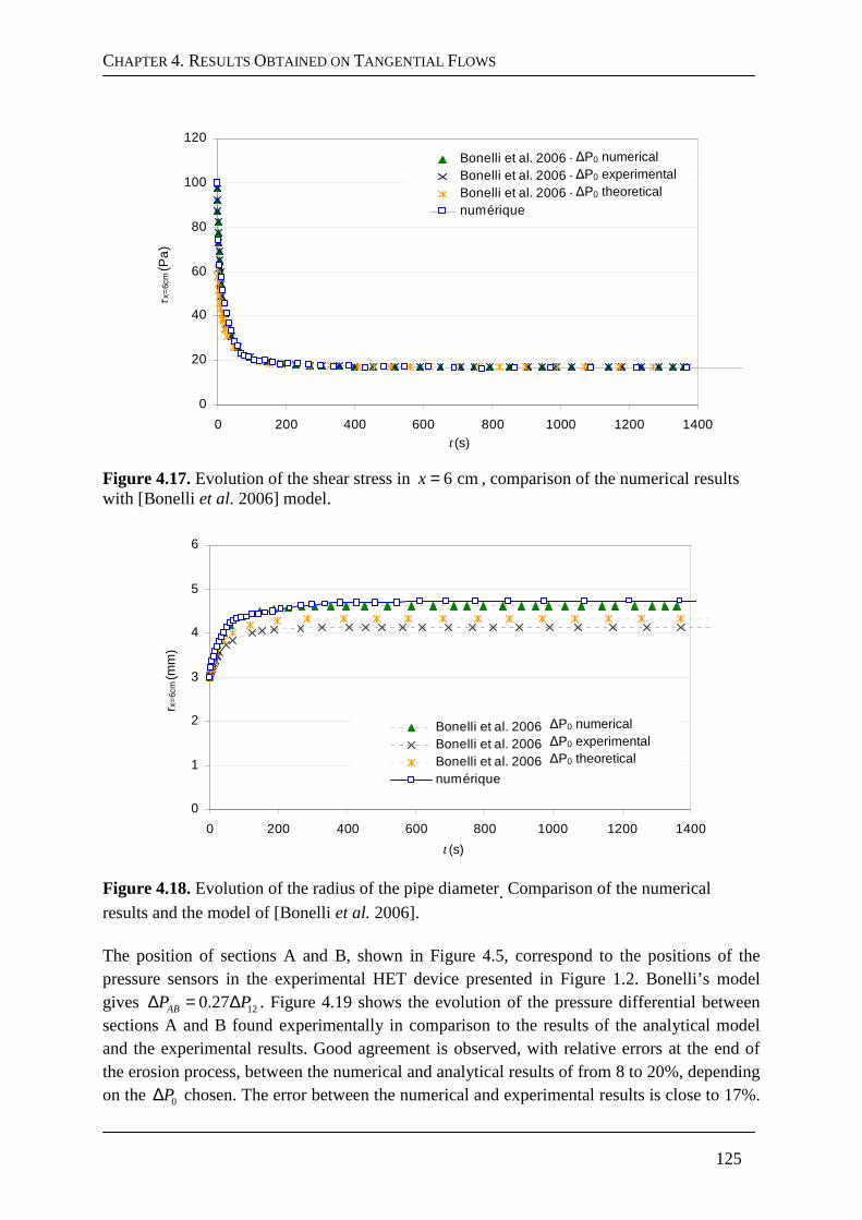
CHAPTER 4. RESULTS OBTAINED ON TANGENTIAL FLOWS
125
0
20
40
60
80
100
120
0 200 400 600 800 1000 1200 1400t (s)
τx=
6cm (
Pa
)Bonelli et al. 2006 - ∆PnumériqueBonelli et al. 2006 - ∆PexpérimentalBonelli et al. 2006 - ∆PBlasiusnumérique
Figure 4.17. Evolution of the shear stress in 6 cmx = , comparison of the numerical results with [Bonelli et al. 2006] model.
0
1
2
3
4
5
6
0 200 400 600 800 1000 1200 1400
t (s)
r x=
6cm (
mm
)
Bonelli et al. 2006 - ∆PnumériqueBonelli et al. 2006 - ∆PexpérimentalBonelli et al. 2006 - ∆PBlasiusnumérique
Figure 4.18. Evolution of the radius of the pipe diameter. Comparison of the numerical
results and the model of [Bonelli et al. 2006]. The position of sections A and B, shown in Figure 4.5, correspond to the positions of the pressure sensors in the experimental HET device presented in Figure 1.2. Bonelli’s model gives 120.27ABP P∆ = ∆ . Figure 4.19 shows the evolution of the pressure differential between sections A and B found experimentally in comparison to the results of the analytical model and the experimental results. Good agreement is observed, with relative errors at the end of the erosion process, between the numerical and analytical results of from 8 to 20%, depending on the 0P∆ chosen. The error between the numerical and experimental results is close to 17%.
∆P0 numerical ∆P0 experimental ∆P0 theoretical
∆P0 numerical ∆P0 experimental ∆P0 theoretical
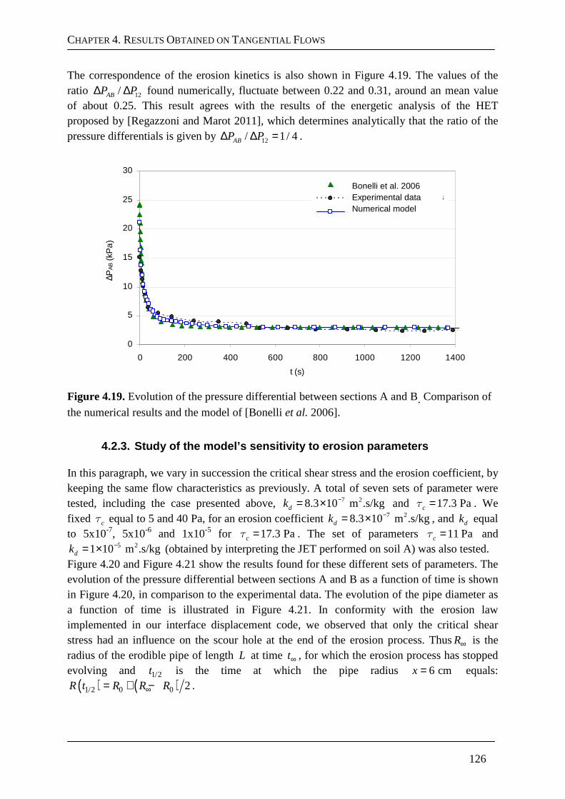
CHAPTER 4. RESULTS OBTAINED ON TANGENTIAL FLOWS
126
The correspondence of the erosion kinetics is also shown in Figure 4.19. The values of the ratio 12/ABP P∆ ∆ found numerically, fluctuate between 0.22 and 0.31, around an mean value of about 0.25. This result agrees with the results of the energetic analysis of the HET proposed by [Regazzoni and Marot 2011], which determines analytically that the ratio of the pressure differentials is given by 12/ 1/ 4ABP P∆ ∆ = .
0
5
10
15
20
25
30
0 200 400 600 800 1000 1200 1400
t (s)
∆P
AB (
kPa
)
Bonelli et al. 2006
données expérimentales
numérique
Figure 4.19. Evolution of the pressure differential between sections A and B. Comparison of
the numerical results and the model of [Bonelli et al. 2006].
4.2.3. Study of the model’s sensitivity to erosion parameters
In this paragraph, we vary in succession the critical shear stress and the erosion coefficient, by keeping the same flow characteristics as previously. A total of seven sets of parameter were tested, including the case presented above, 7 28.3 10 m .s/kgdk −= × and 17.3 Pacτ = . We fixed cτ equal to 5 and 40 Pa, for an erosion coefficient 7 28.3 10 m .s/kgdk −= × , and dk equal to 5x10⁻⁷, 5x10⁻⁶ and 1x10⁻⁵ for 17.3 Pacτ = . The set of parameters 11 Pacτ = and
5 21 10 m .s/kgdk −= × (obtained by interpreting the JET performed on soil A) was also tested. Figure 4.20 and Figure 4.21 show the results found for these different sets of parameters. The evolution of the pressure differential between sections A and B as a function of time is shown in Figure 4.20, in comparison to the experimental data. The evolution of the pipe diameter as a function of time is illustrated in Figure 4.21. In conformity with the erosion law implemented in our interface displacement code, we observed that only the critical shear stress had an influence on the scour hole at the end of the erosion process. ThusR∞ is the radius of the erodible pipe of length L at time t∞ , for which the erosion process has stopped evolving and 1/2t is the time at which the pipe radius 6 cmx = equals:
( ) ( )1/2 0 0 2R t R R R∞= + − .
Bonelli et al. 2006 Experimental data Numerical model
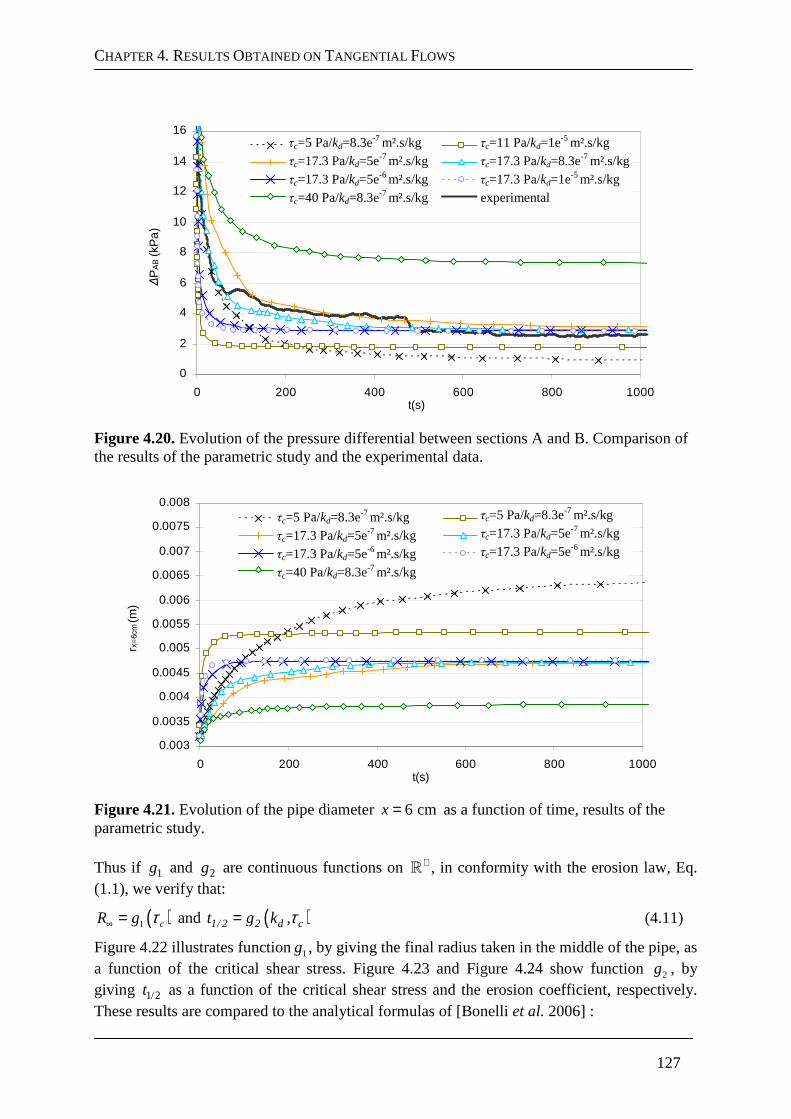
CHAPTER 4. RESULTS OBTAINED ON TANGENTIAL FLOWS
127
0
2
4
6
8
10
12
14
16
0 200 400 600 800 1000t(s)
∆P
AB (
kPa
)tc 5 / kd 8.3e-7 tc 11.0 / kd 1.0e-5 tc 17.3 / kd 5e-7 tc 17.3 / kd 8.3e-7
tc 17.3 / kd 5e-6 tc 17.3 / kd 1e-5 tc 40 / kd 8.3e-7 experimental
Figure 4.20. Evolution of the pressure differential between sections A and B. Comparison of the results of the parametric study and the experimental data.
0.003
0.0035
0.004
0.0045
0.005
0.0055
0.006
0.0065
0.007
0.0075
0.008
0 200 400 600 800 1000t(s)
r x=
6cm (
m)
tc 5 / kd 8.3e-7 tc 11.0 / kd 1.0e-5tc 17.3 / kd 5e-7 tc 17.3 / kd 8.3e-7
tc 17.3 / kd 5e-6 tc 17.3 / kd 1e-5 tc 40 / kd 8.3e-7
Figure 4.21. Evolution of the pipe diameter 6 cmx = as a function of time, results of the parametric study. Thus if 1g and 2g are continuous functions on +ℝ , in conformity with the erosion law, Eq. (1.1), we verify that:
( )1 cR g τ∞ = and ( )1/ 2 2 d ct g k ,τ= (4.11)
Figure 4.22 illustrates function1g , by giving the final radius taken in the middle of the pipe, as a function of the critical shear stress. Figure 4.23 and Figure 4.24 show function 2g , by giving 1/2t as a function of the critical shear stress and the erosion coefficient, respectively. These results are compared to the analytical formulas of [Bonelli et al. 2006] :
τc=5 Pa/kd=8.3e-7 m².s/kg τc=17.3 Pa/kd=5e-7 m².s/kg τc=17.3 Pa/kd=5e-6 m².s/kg τc=40 Pa/kd=8.3e-7 m².s/kg
τc=11 Pa/kd=1e-5 m².s/kg τc=17.3 Pa/kd=8.3e-7 m².s/kg τc=17.3 Pa/kd=1e-5 m².s/kg experimental
τc=5 Pa/kd=8.3e-7 m².s/kg τc=17.3 Pa/kd=5e-7 m².s/kg τc=17.3 Pa/kd=5e-6 m².s/kg τc=40 Pa/kd=8.3e-7 m².s/kg
τc=5 Pa/kd=8.3e-7 m².s/kg τc=17.3 Pa/kd=5e-7 m².s/kg τc=17.3 Pa/kd=5e-6 m².s/kg
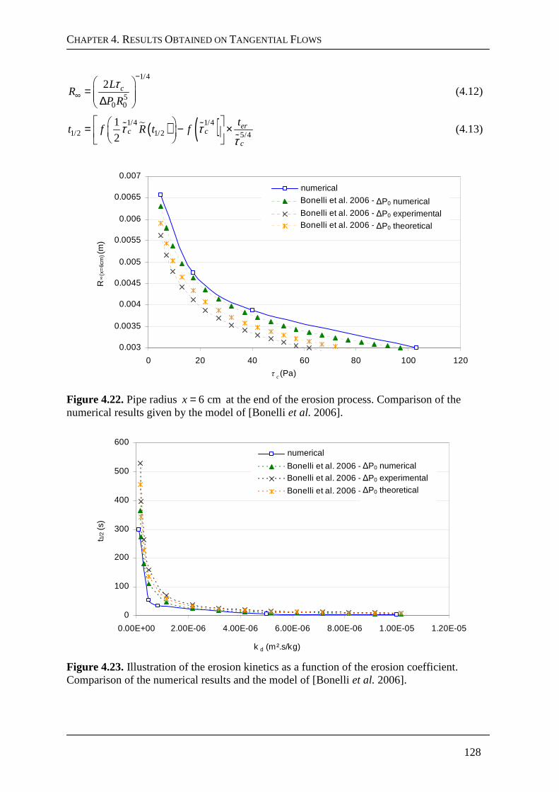
CHAPTER 4. RESULTS OBTAINED ON TANGENTIAL FLOWS
128
1/4
50 0
2 cLR
P R
τ−
∞
= ∆ (4.12)
( ) ( )1/4 1/41/2 1/2 5/4
1
2er
c c
c
tt f R t fτ τ
τ = − ×
ɶ ɶ
ɶ (4.13)
0.003
0.0035
0.004
0.0045
0.005
0.0055
0.006
0.0065
0.007
0 20 40 60 80 100 120
τ c(Pa)
R∞
(x=
6cm
) (m
)
numérique
Bonelli et al. 2006 - ∆Pnum
Bonelli et al. 2006 - ∆PexpBonelli et al. 2006 - ∆PBlasius
Figure 4.22. Pipe radius 6 cmx = at the end of the erosion process. Comparison of the numerical results given by the model of [Bonelli et al. 2006].
0
100
200
300
400
500
600
0.00E+00 2.00E-06 4.00E-06 6.00E-06 8.00E-06 1.00E-05 1.20E-05
k d (m².s/kg)
t 1/2
(s)
numérique
Bonelli et al. 2006 - ∆PnumBonelli et al. 2006 - ∆Pexp
Bonelli et al. 2006 - ∆PBlasius
Figure 4.23. Illustration of the erosion kinetics as a function of the erosion coefficient. Comparison of the numerical results and the model of [Bonelli et al. 2006].
∆P0 numerical ∆P0 experimental
∆P0 theoretical
numerical
∆P0 numerical ∆P0 experimental ∆P0 theoretical
numerical
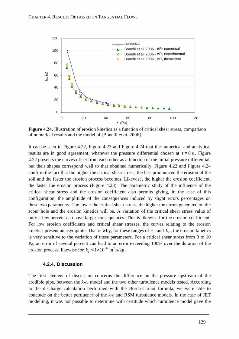
CHAPTER 4. RESULTS OBTAINED ON TANGENTIAL FLOWS
129
0
20
40
60
80
100
120
0 20 40 60 80 100 120τ c(Pa)
t 1/2
(s)
numerical dataBonelli et al. 2006 - ∆PnumBonelli et al. 2006 - ∆PexpBonelli et al. 2006 - ∆PBlasius
Figure 4.24. Illustration of erosion kinetics as a function of critical shear stress, comparison of numerical results and the model of [Bonelli et al. 2006].
It can be seen in Figure 4.22, Figure 4.23 and Figure 4.24 that the numerical and analytical results are in good agreement, whatever the pressure differential chosen at 0 st = . Figure 4.22 presents the curves offset from each other as a function of the initial pressure differential, but their shapes correspond well to that obtained numerically. Figure 4.22 and Figure 4.24 confirm the fact that the higher the critical shear stress, the less pronounced the erosion of the soil and the faster the erosion process becomes. Likewise, the higher the erosion coefficient, the faster the erosion process (Figure 4.23). The parametric study of the influence of the critical shear stress and the erosion coefficient also permits giving, in the case of this configuration, the amplitude of the consequences induced by slight errors percentages on these two parameters. The lower the critical shear stress, the higher the errors generated on the scour hole and the erosion kinetics will be. A variation of the critical shear stress value of only a few percent can have larger consequences. This is likewise for the erosion coefficient. For low erosion coefficients and critical shear stresses, the curves relating to the erosion kinetics present an asymptote. That is why, for these ranges of cτ and dk , the erosion kinetics is very sensitive to the variation of these parameters. For a critical shear stress from 0 to 10 Pa, an error of several percent can lead to an error exceeding 100% over the duration of the erosion process; likewise for 6 21 10 m .s/kgdk −< × .
4.2.4. Discussion
The first element of discussion concerns the difference on the pressure upstream of the erodible pipe, between the k-ω model and the two other turbulence models tested. According to the discharge calculation performed with the Borda-Carnot formula, we were able to conclude on the better pertinence of the k-ε and RSM turbulence models. In the case of JET modelling, it was not possible to determine with certitude which turbulence model gave the
∆P0 numerical ∆P0 experimental ∆P0 theoretical
numerical
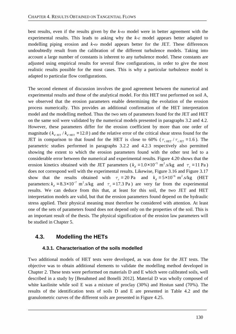
CHAPTER 4. RESULTS OBTAINED ON TANGENTIAL FLOWS
130
best results, even if the results given by the k-ω model were in better agreement with the experimental results. This leads to asking why the k-ε model appears better adapted to modelling piping erosion and k-ω model appears better for the JET. These differences undoubtedly result from the calibration of the different turbulence models. Taking into account a large number of constants is inherent to any turbulence model. These constants are adjusted using empirical results for several flow configurations, in order to give the most realistic results possible for the most cases. This is why a particular turbulence model is adapted to particular flow configurations. The second element of discussion involves the good agreement between the numerical and experimental results and those of the analytical model. For this HET test performed on soil A, we observed that the erosion parameters enable determining the evolution of the erosion process numerically. This provides an additional confirmation of the HET interpretation model and the modelling method. Thus the two sets of parameters found for the JET and HET on the same soil were validated by the numerical models presented in paragraphs 3.2 and 4.2. However, these parameters differ for the erosion coefficient by more than one order of magnitude ( JET HET/ 12.0d dk k = ) and the relative error of the critical shear stress found for the JET in comparison to that found for the HET is close to 60% ( c HET c JET/ 1.6τ τ = ). The parametric studies performed in paragraphs 3.2.2 and 4.2.3 respectively also permitted showing the extent to which the erosion parameters found with the other test led to a considerable error between the numerical and experimental results. Figure 4.20 shows that the erosion kinetics obtained with the JET parameters ( 5 21.0 10 m .s/kgdk −= × and 11 Pacτ = ) does not correspond well with the experimental results. Likewise, Figure 3.16 and Figure 3.17 show that the results obtained with 20 Pacτ = and 6 25 10 m .s/kgdk −= × (HET parameters: 7 28.3 10 m .s/kgdk −= × and 17.3 Pacτ = ) are very far from the experimental results. We can deduce from this that, at least for this soil, the two JET and HET interpretation models are valid, but that the erosion parameters found depend on the hydraulic stress applied. Their physical meaning must therefore be considered with attention. At least one of the sets of parameters found does not depend only on the properties of the soil. This is an important result of the thesis. The physical signification of the erosion law parameters will be studied in Chapter 5.
4.3. Modelling the HETs
4.3.1. Characterisation of the soils modelled
Two additional models of HET tests were developed, as was done for the JET tests. The objective was to obtain additional elements to validate the modelling method developed in Chapter 2. These tests were performed on materials D and E which were calibrated soils, well described in a study by [Benahmed and Bonelli 2012]. Material D was wholly composed of white kaolinite while soil E was a mixture of proclay (30%) and Hostun sand (70%). The results of the identification tests of soils D and E are presented in Table 4.2 and the granulometric curves of the different soils are presented in Figure 4.25.
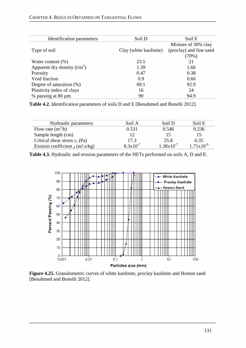
CHAPTER 4. RESULTS OBTAINED ON TANGENTIAL FLOWS
131
Identification parameters Soil D Soil E
Type of soil Clay (white kaolinite) Mixture of 30% clay
(proclay) and fine sand (70%)
Water content (%) 23.5 21 Apparent dry density (t/m3) 1.39 1.66 Porosity 0.47 0.38 Void fraction 0.9 0.60 Degree of saturation (%) 69.1 92.9 Plasticity index of clays 16 24 % passing at 80 µm 90 94.9
Table 4.2. Identification parameters of soils D and E [Benahmed and Bonelli 2012].
Hydraulic parameters Soil A Soil D Soil E Flow rate (m3/h) 0.531 0.546 0.236 Sample length (cm) 12 15 15 Critical shear stress τc (Pa) 17.3 25.8 6.35 Erosion coefficient d (m².s/kg) 8.3x10⁻⁷ 1.38x10⁻⁷ 1.71x10⁻⁶
Table 4.3. Hydraulic and erosion parameters of the HETs performed on soils A, D and E.
Figure 4.25. Granulometric curves of white kaolinite, proclay kaolinite and Hostun sand [Benahmed and Bonelli 2012].
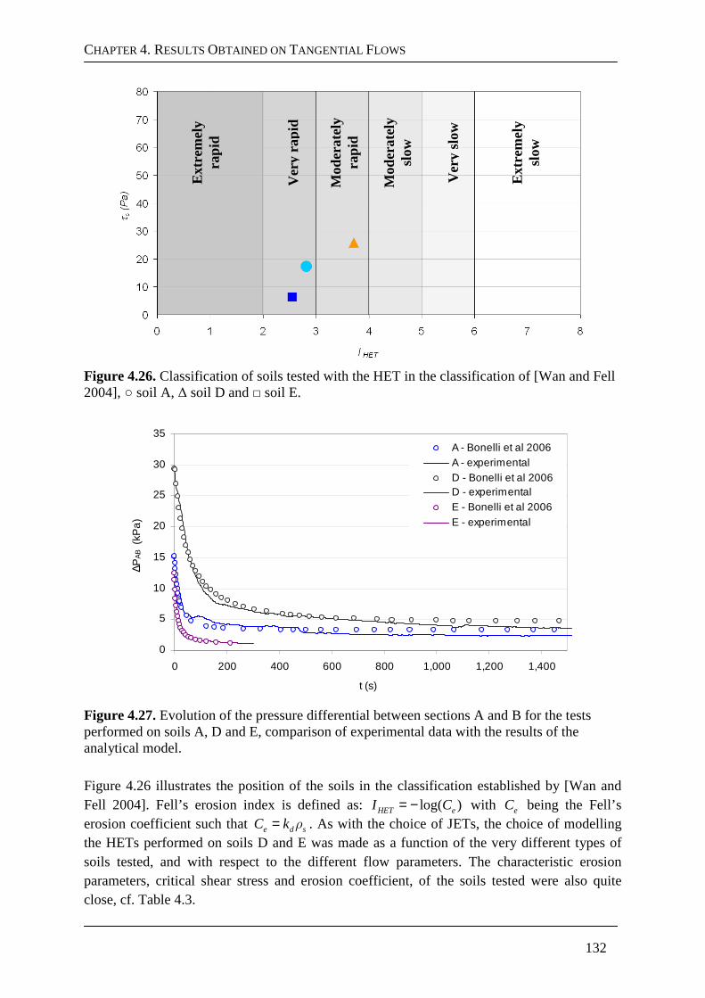
CHAPTER 4. RESULTS OBTAINED ON TANGENTIAL FLOWS
132
Figure 4.26. Classification of soils tested with the HET in the classification of [Wan and Fell 2004], soil A, ∆ soil D and soil E.
0
5
10
15
20
25
30
35
0 200 400 600 800 1,000 1,200 1,400
t (s)
∆P
AB (
kPa
)
A - Bonelli et al 2006A - experimentalD - Bonelli et al 2006D - experimentalE - Bonelli et al 2006E - experimental
Figure 4.27. Evolution of the pressure differential between sections A and B for the tests performed on soils A, D and E, comparison of experimental data with the results of the analytical model. Figure 4.26 illustrates the position of the soils in the classification established by [Wan and Fell 2004]. Fell’s erosion index is defined as: log( )HET eI C= − with eC being the Fell’s erosion coefficient such that e d sC k ρ= . As with the choice of JETs, the choice of modelling the HETs performed on soils D and E was made as a function of the very different types of soils tested, and with respect to the different flow parameters. The characteristic erosion parameters, critical shear stress and erosion coefficient, of the soils tested were also quite close, cf. Table 4.3.
Ext
rem
ely
rapi
d
Ver
y ra
pid
Mod
erat
ely
rapi
d
Mod
erat
ely
slow
Ver
y sl
ow
Ext
rem
ely
slow
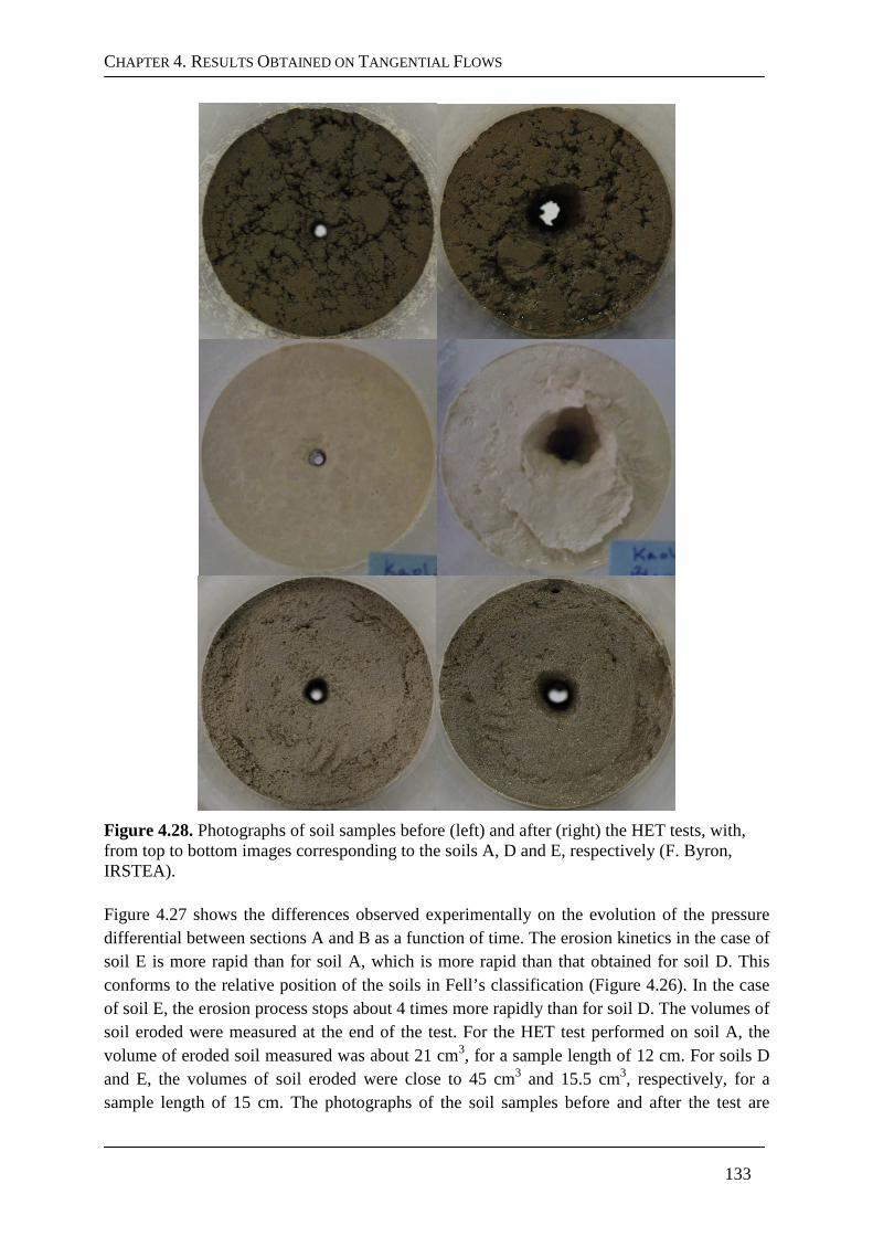
CHAPTER 4. RESULTS OBTAINED ON TANGENTIAL FLOWS
133
Figure 4.28. Photographs of soil samples before (left) and after (right) the HET tests, with, from top to bottom images corresponding to the soils A, D and E, respectively (F. Byron, IRSTEA). Figure 4.27 shows the differences observed experimentally on the evolution of the pressure differential between sections A and B as a function of time. The erosion kinetics in the case of soil E is more rapid than for soil A, which is more rapid than that obtained for soil D. This conforms to the relative position of the soils in Fell’s classification (Figure 4.26). In the case of soil E, the erosion process stops about 4 times more rapidly than for soil D. The volumes of soil eroded were measured at the end of the test. For the HET test performed on soil A, the volume of eroded soil measured was about 21 cm3, for a sample length of 12 cm. For soils D and E, the volumes of soil eroded were close to 45 cm3 and 15.5 cm3, respectively, for a sample length of 15 cm. The photographs of the soil samples before and after the test are
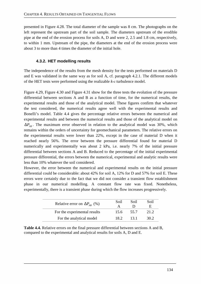
CHAPTER 4. RESULTS OBTAINED ON TANGENTIAL FLOWS
134
presented in Figure 4.28. The total diameter of the sample was 8 cm. The photographs on the left represent the upstream part of the soil sample. The diameters upstream of the erodible pipe at the end of the erosion process for soils A, D and were 2, 2.5 and 1.8 cm, respectively, to within 1 mm. Upstream of the pipe, the diameters at the end of the erosion process were about 3 to more than 4 times the diameter of the initial hole.
4.3.2. HET modelling results
The independence of the results from the mesh density for the tests performed on materials D and E was validated in the same way as for soil A, cf. paragraph 4.2.1. The different models of the HET tests were performed using the realizable k-ε turbulence model. Figure 4.29, Figure 4.30 and Figure 4.31 show for the three tests the evolution of the pressure differential between sections A and B as a function of time, for the numerical results, the experimental results and those of the analytical model. These figures confirm that whatever the test considered, the numerical results agree well with the experimental results and Bonelli’s model. Table 4.4 gives the percentage relative errors between the numerical and experimental results and between the numerical results and those of the analytical model on
ABP∆ . The maximum error observed in relation to the analytical model was 30%, which remains within the orders of uncertainty for geomechanical parameters. The relative errors on the experimental results were lower than 22%, except in the case of material D when it reached nearly 56%. The error between the pressure differential found for material D numerically and experimentally was about 2 kPa, i.e. nearly 7% of the initial pressure differential between sections A and B. Reduced to the percentage of the initial experimental pressure differential, the errors between the numerical, experimental and analytic results were less than 10% whatever the soil considered. However, the error between the numerical and experimental results on the initial pressure differential could be considerable: about 42% for soil A, 12% for D and 57% for soil E. These errors were certainly due to the fact that we did not consider a transient flow establishment phase in our numerical modelling. A constant flow rate was fixed. Nonetheless, experimentally, there is a transient phase during which the flow increases progressively.
Relative error on ABP∆ (%) Soil A
Soil D
Soil E
For the experimental results 15.6 55.7 21.2
For the analytical model 18.2 13.1 30.2
Table 4.4. Relative errors on the final pressure differential between sections A and B, compared to the experimental and analytical results for soils A, D and E.
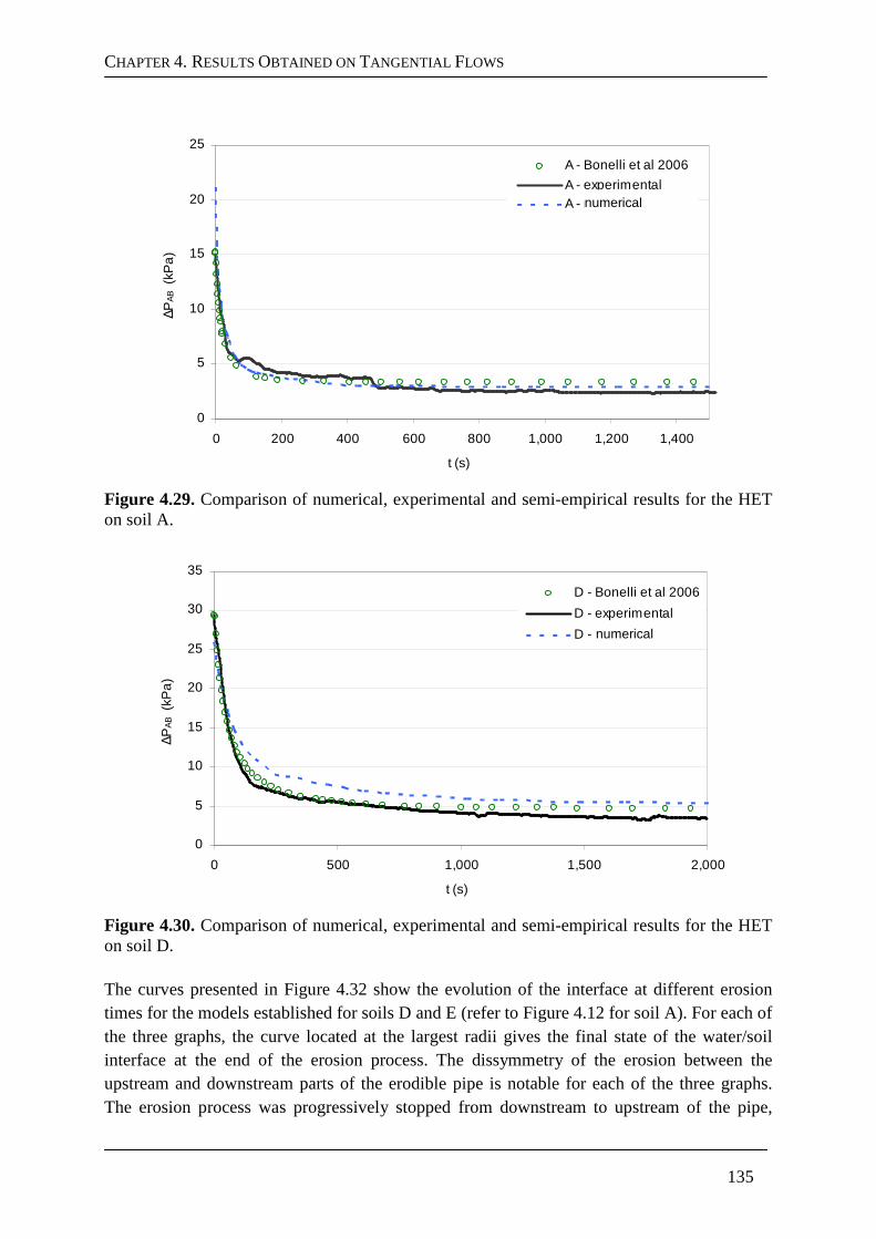
CHAPTER 4. RESULTS OBTAINED ON TANGENTIAL FLOWS
135
0
5
10
15
20
25
0 200 400 600 800 1,000 1,200 1,400
t (s)
∆P
AB (
kPa
)A - Bonelli et al 2006
A - experimentalA - numerique
Figure 4.29. Comparison of numerical, experimental and semi-empirical results for the HET on soil A.
0
5
10
15
20
25
30
35
0 500 1,000 1,500 2,000
t (s)
∆P
AB (
kPa
)
D - Bonelli et al 2006
D - experimental
D - numérique
Figure 4.30. Comparison of numerical, experimental and semi-empirical results for the HET on soil D. The curves presented in Figure 4.32 show the evolution of the interface at different erosion times for the models established for soils D and E (refer to Figure 4.12 for soil A). For each of the three graphs, the curve located at the largest radii gives the final state of the water/soil interface at the end of the erosion process. The dissymmetry of the erosion between the upstream and downstream parts of the erodible pipe is notable for each of the three graphs. The erosion process was progressively stopped from downstream to upstream of the pipe,
numerical
numerical
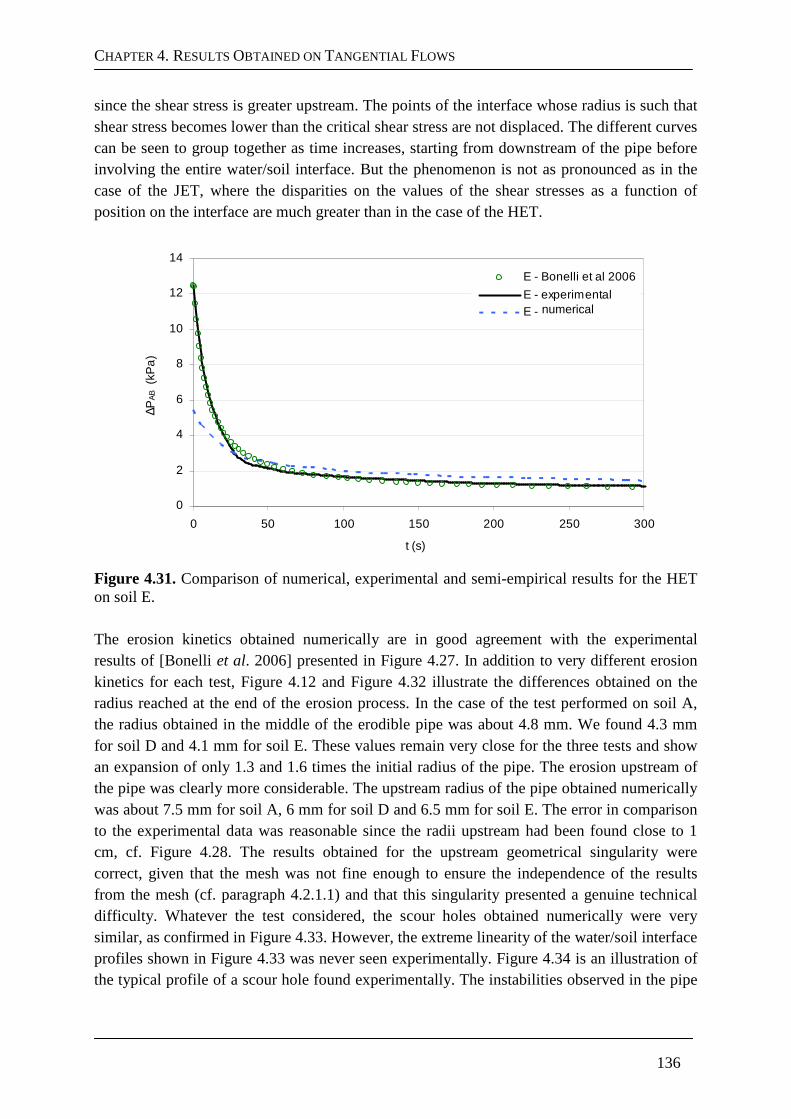
CHAPTER 4. RESULTS OBTAINED ON TANGENTIAL FLOWS
136
since the shear stress is greater upstream. The points of the interface whose radius is such that shear stress becomes lower than the critical shear stress are not displaced. The different curves can be seen to group together as time increases, starting from downstream of the pipe before involving the entire water/soil interface. But the phenomenon is not as pronounced as in the case of the JET, where the disparities on the values of the shear stresses as a function of position on the interface are much greater than in the case of the HET.
0
2
4
6
8
10
12
14
0 50 100 150 200 250 300
t (s)
∆P
AB (
kPa
)
E - Bonelli et al 2006
E - experimentalE - numerique
Figure 4.31. Comparison of numerical, experimental and semi-empirical results for the HET on soil E. The erosion kinetics obtained numerically are in good agreement with the experimental results of [Bonelli et al. 2006] presented in Figure 4.27. In addition to very different erosion kinetics for each test, Figure 4.12 and Figure 4.32 illustrate the differences obtained on the radius reached at the end of the erosion process. In the case of the test performed on soil A, the radius obtained in the middle of the erodible pipe was about 4.8 mm. We found 4.3 mm for soil D and 4.1 mm for soil E. These values remain very close for the three tests and show an expansion of only 1.3 and 1.6 times the initial radius of the pipe. The erosion upstream of the pipe was clearly more considerable. The upstream radius of the pipe obtained numerically was about 7.5 mm for soil A, 6 mm for soil D and 6.5 mm for soil E. The error in comparison to the experimental data was reasonable since the radii upstream had been found close to 1 cm, cf. Figure 4.28. The results obtained for the upstream geometrical singularity were correct, given that the mesh was not fine enough to ensure the independence of the results from the mesh (cf. paragraph 4.2.1.1) and that this singularity presented a genuine technical difficulty. Whatever the test considered, the scour holes obtained numerically were very similar, as confirmed in Figure 4.33. However, the extreme linearity of the water/soil interface profiles shown in Figure 4.33 was never seen experimentally. Figure 4.34 is an illustration of the typical profile of a scour hole found experimentally. The instabilities observed in the pipe
numerical
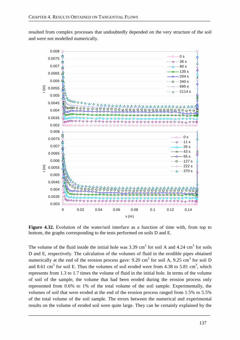
CHAPTER 4. RESULTS OBTAINED ON TANGENTIAL FLOWS
137
resulted from complex processes that undoubtedly depended on the very structure of the soil and were not modelled numerically.
0.003
0.0035
0.004
0.0045
0.005
0.0055
0.006
0.0065
0.007
0.0075
0.008
r (m
)
0 s36 s80 s135 s204 s340 s695 s2114 s
0.003
0.0035
0.004
0.0045
0.005
0.0055
0.006
0.0065
0.007
0.0075
0.008
0 0.02 0.04 0.06 0.08 0.1 0.12 0.14
x (m)
r (m
)
0 s11 s26 s43 s65 s127 s222 s370 s
Figure 4.32. Evolution of the water/soil interface as a function of time with, from top to bottom, the graphs corresponding to the tests performed on soils D and E.
The volume of the fluid inside the initial hole was 3.39 cm3 for soil A and 4.24 cm3 for soils D and E, respectively. The calculation of the volumes of fluid in the erodible pipes obtained numerically at the end of the erosion process gave: 9.20 cm3 for soil A, 9.25 cm3 for soil D and 8.61 cm3 for soil E. Thus the volumes of soil eroded were from 4.38 to 5.81 cm3, which represents from 1.3 to 1.7 times the volume of fluid in the initial hole. In terms of the volume of soil of the sample, the volume that had been eroded during the erosion process only represented from 0.6% to 1% of the total volume of the soil sample. Experimentally, the volumes of soil that were eroded at the end of the erosion process ranged from 1.5% to 5.5% of the total volume of the soil sample. The errors between the numerical and experimental results on the volume of eroded soil were quite large. They can be certainly explained by the
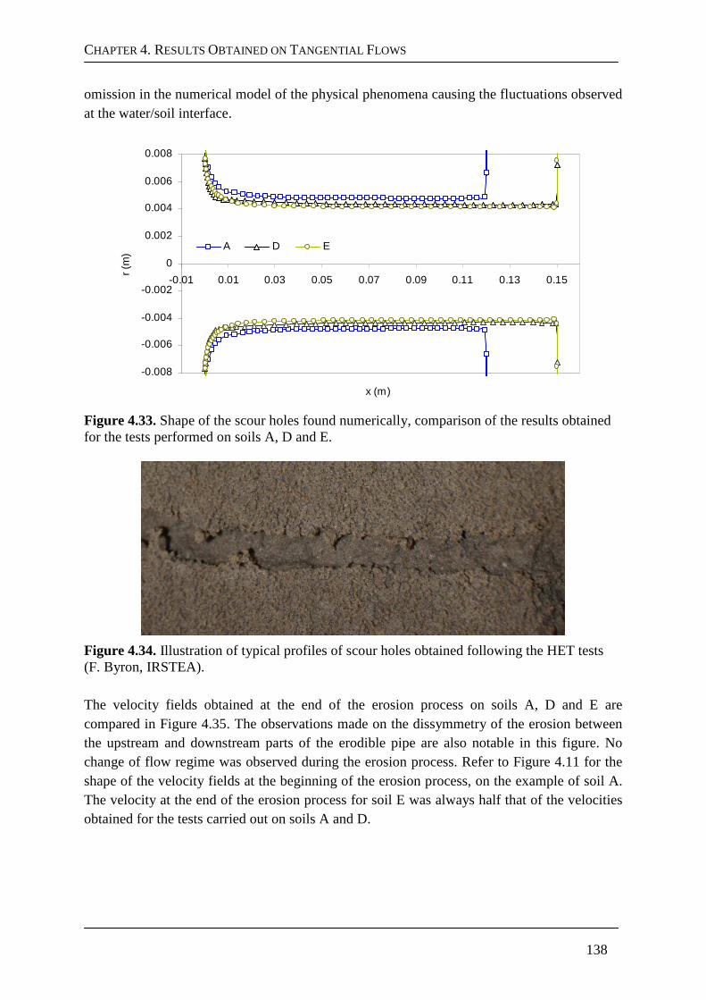
CHAPTER 4. RESULTS OBTAINED ON TANGENTIAL FLOWS
138
omission in the numerical model of the physical phenomena causing the fluctuations observed at the water/soil interface.
-0.008
-0.006
-0.004
-0.002
0
0.002
0.004
0.006
0.008
-0.01 0.01 0.03 0.05 0.07 0.09 0.11 0.13 0.15
x (m)
r (m
)
A D E
Figure 4.33. Shape of the scour holes found numerically, comparison of the results obtained for the tests performed on soils A, D and E.
Figure 4.34. Illustration of typical profiles of scour holes obtained following the HET tests (F. Byron, IRSTEA). The velocity fields obtained at the end of the erosion process on soils A, D and E are compared in Figure 4.35. The observations made on the dissymmetry of the erosion between the upstream and downstream parts of the erodible pipe are also notable in this figure. No change of flow regime was observed during the erosion process. Refer to Figure 4.11 for the shape of the velocity fields at the beginning of the erosion process, on the example of soil A. The velocity at the end of the erosion process for soil E was always half that of the velocities obtained for the tests carried out on soils A and D.
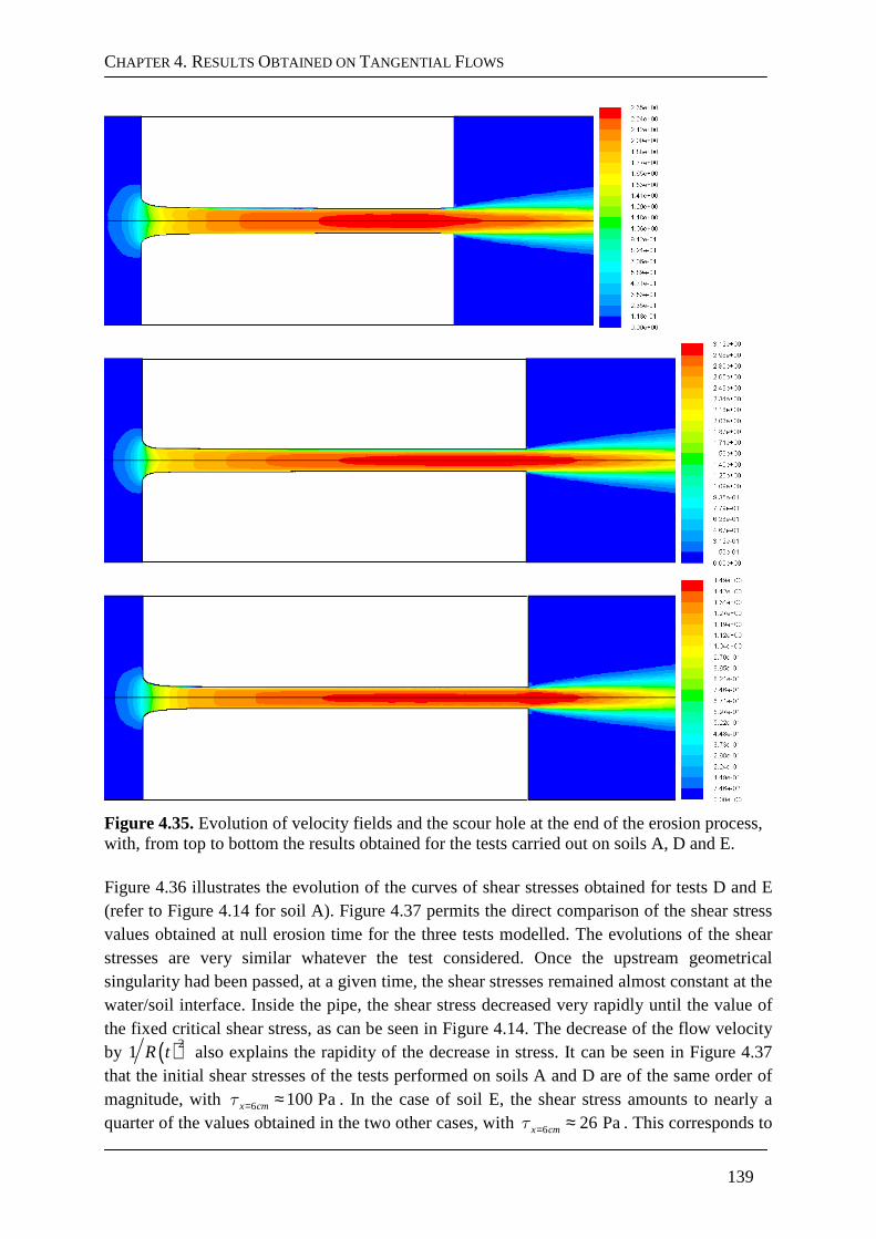
CHAPTER 4. RESULTS OBTAINED ON TANGENTIAL FLOWS
139
Figure 4.35. Evolution of velocity fields and the scour hole at the end of the erosion process, with, from top to bottom the results obtained for the tests carried out on soils A, D and E. Figure 4.36 illustrates the evolution of the curves of shear stresses obtained for tests D and E (refer to Figure 4.14 for soil A). Figure 4.37 permits the direct comparison of the shear stress values obtained at null erosion time for the three tests modelled. The evolutions of the shear stresses are very similar whatever the test considered. Once the upstream geometrical singularity had been passed, at a given time, the shear stresses remained almost constant at the water/soil interface. Inside the pipe, the shear stress decreased very rapidly until the value of the fixed critical shear stress, as can be seen in Figure 4.14. The decrease of the flow velocity by ( )2
1 R t also explains the rapidity of the decrease in stress. It can be seen in Figure 4.37 that the initial shear stresses of the tests performed on soils A and D are of the same order of magnitude, with 6 100 Pax cmτ = ≈ . In the case of soil E, the shear stress amounts to nearly a quarter of the values obtained in the two other cases, with 6 26 Pax cmτ = ≈ . This corresponds to
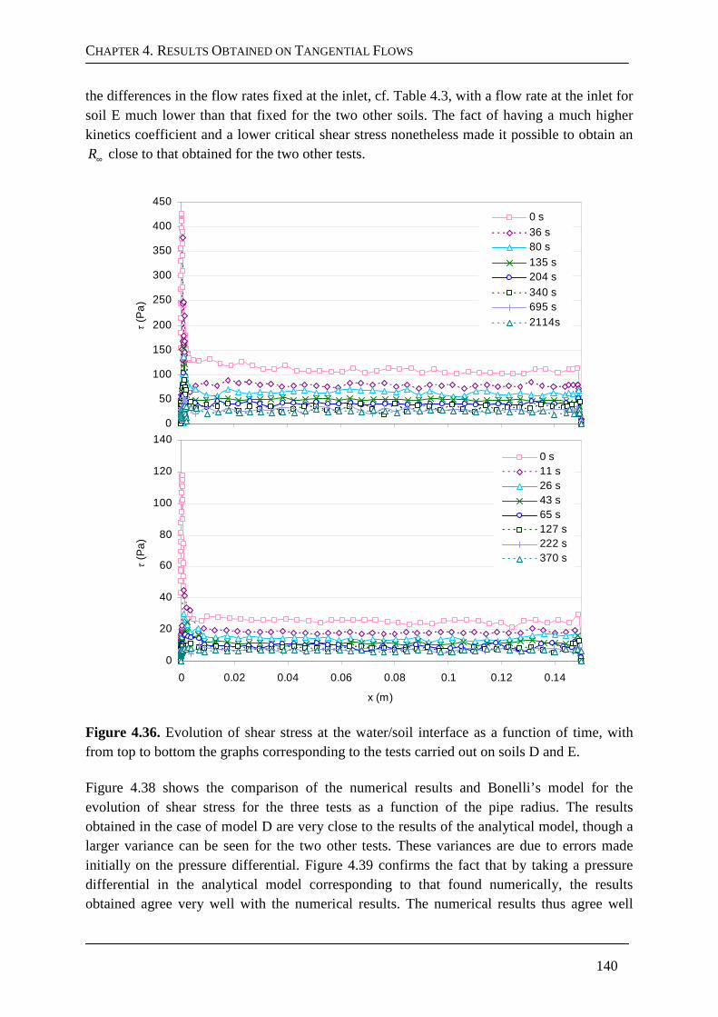
CHAPTER 4. RESULTS OBTAINED ON TANGENTIAL FLOWS
140
the differences in the flow rates fixed at the inlet, cf. Table 4.3, with a flow rate at the inlet for soil E much lower than that fixed for the two other soils. The fact of having a much higher kinetics coefficient and a lower critical shear stress nonetheless made it possible to obtain an R∞ close to that obtained for the two other tests.
0
50
100
150
200
250
300
350
400
450
τ (
Pa
)
0 s36 s80 s135 s204 s340 s695 s2114s
0
20
40
60
80
100
120
140
0 0.02 0.04 0.06 0.08 0.1 0.12 0.14
x (m)
τ (
Pa
)
0 s11 s26 s43 s65 s127 s222 s370 s
Figure 4.36. Evolution of shear stress at the water/soil interface as a function of time, with from top to bottom the graphs corresponding to the tests carried out on soils D and E.
Figure 4.38 shows the comparison of the numerical results and Bonelli’s model for the evolution of shear stress for the three tests as a function of the pipe radius. The results obtained in the case of model D are very close to the results of the analytical model, though a larger variance can be seen for the two other tests. These variances are due to errors made initially on the pressure differential. Figure 4.39 confirms the fact that by taking a pressure differential in the analytical model corresponding to that found numerically, the results obtained agree very well with the numerical results. The numerical results thus agree well
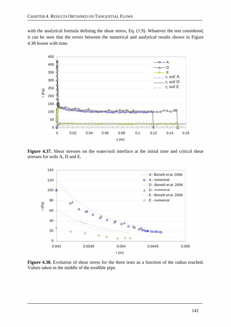
CHAPTER 4. RESULTS OBTAINED ON TANGENTIAL FLOWS
141
with the analytical formula defining the shear stress, Eq. (1.9). Whatever the test considered, it can be seen that the errors between the numerical and analytical results shown in Figure 4.38 lessen with time.
0
50
100
150
200
250
300
350
400
450
0 0.02 0.04 0.06 0.08 0.1 0.12 0.14 0.16
x (m)
τ (P
a)
A
DE
tauc Atauc D
tauc E
Figure 4.37. Shear stresses on the water/soil interface at the initial time and critical shear stresses for soils A, D and E.
0
20
40
60
80
100
120
140
0.003 0.0035 0.004 0.0045 0.005
r (m)
τ (P
a)
A - Bonelli et al. 2006
A - numeriqueD - Bonelli et al. 2006
D - numeriqueE - Bonelli et al. 2006
E - numerique
Figure 4.38. Evolution of shear stress for the three tests as a function of the radius reached. Values taken in the middle of the erodible pipe.
τc soil A τc soil D τc soil E
numerical
numerical
numerical
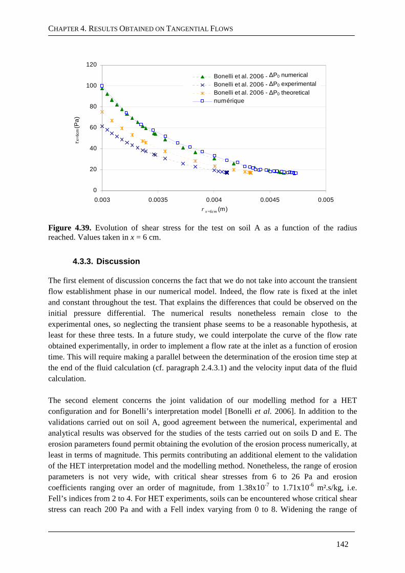
CHAPTER 4. RESULTS OBTAINED ON TANGENTIAL FLOWS
142
0
20
40
60
80
100
120
0.003 0.0035 0.004 0.0045 0.005
r x=6cm(m)
τx=
6cm (
Pa
)Bonelli et al. 2006 - ∆PnumériqueBonelli et al. 2006 - ∆PexpérimentalBonelli et al. 2006 - ∆PBlasiusnumérique
Figure 4.39. Evolution of shear stress for the test on soil A as a function of the radius reached. Values taken in x = 6 cm.
4.3.3. Discussion
The first element of discussion concerns the fact that we do not take into account the transient flow establishment phase in our numerical model. Indeed, the flow rate is fixed at the inlet and constant throughout the test. That explains the differences that could be observed on the initial pressure differential. The numerical results nonetheless remain close to the experimental ones, so neglecting the transient phase seems to be a reasonable hypothesis, at least for these three tests. In a future study, we could interpolate the curve of the flow rate obtained experimentally, in order to implement a flow rate at the inlet as a function of erosion time. This will require making a parallel between the determination of the erosion time step at the end of the fluid calculation (cf. paragraph 2.4.3.1) and the velocity input data of the fluid calculation. The second element concerns the joint validation of our modelling method for a HET configuration and for Bonelli’s interpretation model [Bonelli et al. 2006]. In addition to the validations carried out on soil A, good agreement between the numerical, experimental and analytical results was observed for the studies of the tests carried out on soils D and E. The erosion parameters found permit obtaining the evolution of the erosion process numerically, at least in terms of magnitude. This permits contributing an additional element to the validation of the HET interpretation model and the modelling method. Nonetheless, the range of erosion parameters is not very wide, with critical shear stresses from 6 to 26 Pa and erosion coefficients ranging over an order of magnitude, from 1.38x10⁻⁷ to 1.71x10⁻⁶ m².s/kg, i.e. Fell’s indices from 2 to 4. For HET experiments, soils can be encountered whose critical shear stress can reach 200 Pa and with a Fell index varying from 0 to 8. Widening the range of
∆P0 numerical
∆P0 experimental ∆P0 theoretical
CHAPTER 4. RESULTS OBTAINED ON TANGENTIAL FLOWS
143
erosion parameters of the tests modelled could be included in the perspectives of this Ph.D. thesis work. The third element of discussion concerns the comparison of the results obtained from the JETs and HETs. Indeed, the quantities of soil eroded during a HET test were much lower than the quantities eroded during a JET, in the order of one magnitude in volume. Also, the evolution of flow as a function of time is less complex in the case of HET, since no change of regime was observed. On the contrary, our numerical model could explain the non negligible fluctuations observed experimentally on the water/soil interface. To widen the representativeness of the soils tested as much as possible, and because the initial objective of the thesis was to model the JET, the choice was made to model real soils which, it turned out, had not been tested by the HET, apart from soil A. This explains that the four other tests modelled were not performed on the same soils. One of the perspectives of this thesis work could be to model more tests performed on the same soil by the JET and the HET. However, the orders of magnitude of the erosion parameters found with the JET and the HET were validated by modelling. This provides an additional element to the need to examine the physical signification of the erosion parameters defined in the erosion law (1.1).
4.4. Conclusions of the application to piping flows
In this chapter, the modelling method developed was applied to concentrated leak erosion. Firstly, the numerical model was confronted by a theoretical validation for the case of a Poiseuille flow with erosion. The flow rate of the flow was constant, implying an exponential evolution of the pipe diameter. The numerical results obtained agree very well with the theoretical results, with a relative error of less than 2%. Secondly, a HET test was modelled and the results obtained were compared in-depth with Bonelli’s analytical model [Bonelli et al. 2006]. The independence of the results from mesh density was validated. The influence of the turbulence model was studied and the results obtained for the ε−k , ω−k and RSM models proved to be very similar. The results obtained without erosion were compared to the results in the literature and good agreement was reached, with the exception of the result on the pressure upstream, overestimated by the
ω−k model. The models with erosion were therefore only performed with the ε−k model. The numerical results obtained showed good agreement with the experimental results and the analytical model. The study of the numerical model’s sensitivity to erosion parameters was performed. It showed that the erosion parameters obtained with the HET led to accurate modelling of the evolution of the pressure differential in comparison to experimental and analytical results. Then, the discussion raised the fact that the modelling method can be adapted to very varied flow configurations, provided that the turbulence model chosen is adapted too. Thus this study contributed important elements for the validation of the modelling method and the HET interpretation model. Thus the problem of the physical signification of the erosion parameters was dealt with.
CHAPTER 4. RESULTS OBTAINED ON TANGENTIAL FLOWS
144
Thirdly, two additional HETs were modelled. The description of the soils highlighted that they were of very different types. The range of erosion parameters was quite narrow but remained representative, whereas a wide range of hydraulic parameters was implemented. The results obtained agreed well with the experimental and analytical results. The scour holes and flows were compared with each other and with the experimental results. Good agreement was also obtained. The discussion on these results first concerned the fact that, in our models, we did not take the flow establishment phase into account. The agreement between the numerical and experimental results could perhaps be improved still further by taking this phase into account at the beginning of the erosion process. It can be concluded that additional elements for validating the modelling method and interpretation model were provided. The results obtained in Chapter 4 were the subject of a publication. [Mercier et al. submitted-c] describes the modelling of tangential flows. Following the modelling results presented in Chapters 3 and 4, we were able to deduce the following important results: i) the method of modelling the erosion of a cohesive soil by a turbulent flow developed in Chapter 2 was validated in the jet and piping flow configurations; ii) the JET and HET interpretation models were validated, at least in terms of orders of magnitude and within the range of erosion parameters tested; iii) the erosion parameters defined by the so-called classical law are not intrinsic to soil but dependent at least on the orientation of the flow. Therefore much research still remains necessary to better understand the physics of erosion, and explain in particular why the erosion parameters obtained with the Jet Erosion Test can be different from those obtained with the Hole Erosion Test. Chapter 5 presents reflections on the differences between the JET and the HET, and also on the flow parameters that distinguish a normal flow from a tangential flow. Certain paths for improving the erosion law will be described.
145
Chapter 5.
Study of the erosion law
Major elements for validating the JET and HET interpretation models were contributed in Chapters 3 and 4. It was deduced that the erosion parameters found following the JET and HET tests depended on the flow and its orientation in relation to the water/soil interface. The objective of this chapter is to provide elements of response to the physical signification of the erosion parameters and paths for improving the erosion law which would result in formulating a unified representation of soil erodibility. First, an in-depth study of the differences observed for the erosion parameters obtained experimentally following the JET and HET tests is performed. We seek to know if the trends are significant. Then, a numerical study of the signature of the flows according to the angle of impingement is performed. The aim is to determine the flow variables which will vary considerably as a function of this angle. The last part of this thesis will deal with paths for improving the erosion law. Elements of response to this complex problem will be provided.
5.1. Differences between JET and HET for erosion pa rameters
5.1.1. Experimental and literature data
For the same soil tested, the results obtained on the erosion parameters following the Hole and Jet Erosion Tests can differ by a factor of 100. This has been confirmed by the results obtained by [Regazzoni et al. 2008], and by [Wahl et al. 2008], as well as the test campaigns performed jointly by IRSTEA and geophyConsult, cf. Table 5.1. In addition to the considerable differences regarding the orders of magnitude of erosion parameters, it can be seen in Table 5.2 that the relative position of soils with each other is not the same for the JET and HET tests. For example, the soil labelled R_f was considered as resistant in the classification relating to the JET. Its erosion velocity is, however, considered as extremely rapid in the classification linked to the HET. [Regazzoni et al. 2008] used the model developed by [Hanson and Cook 2004] to interpret their JETs and that of [Wan and Fell 2004] for the HETs. [Wahl et al. 2008] also used the interpretation model of [Hanson and Cook 2004] for the JETs, but that of [Bonelli et al. 2006]
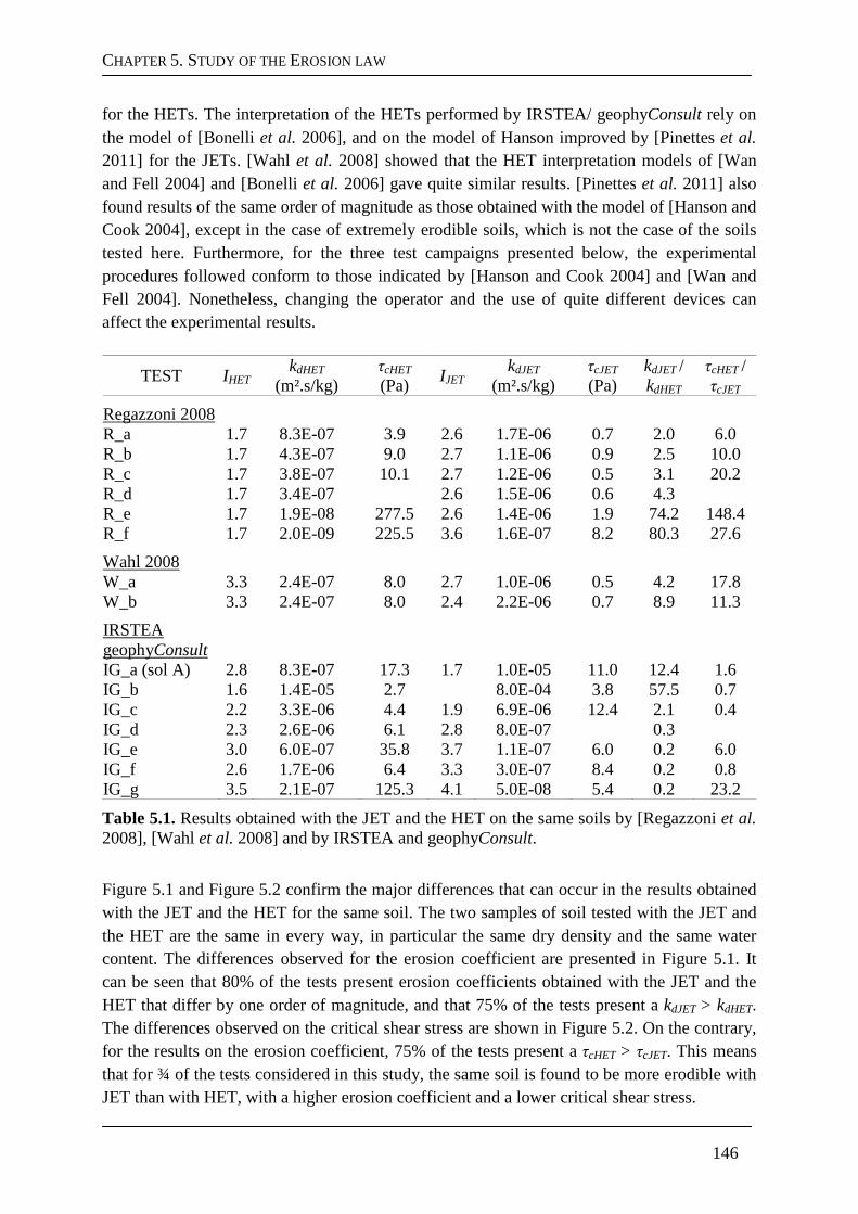
CHAPTER 5. STUDY OF THE EROSION LAW
146
for the HETs. The interpretation of the HETs performed by IRSTEA/ geophyConsult rely on the model of [Bonelli et al. 2006], and on the model of Hanson improved by [Pinettes et al. 2011] for the JETs. [Wahl et al. 2008] showed that the HET interpretation models of [Wan and Fell 2004] and [Bonelli et al. 2006] gave quite similar results. [Pinettes et al. 2011] also found results of the same order of magnitude as those obtained with the model of [Hanson and Cook 2004], except in the case of extremely erodible soils, which is not the case of the soils tested here. Furthermore, for the three test campaigns presented below, the experimental procedures followed conform to those indicated by [Hanson and Cook 2004] and [Wan and Fell 2004]. Nonetheless, changing the operator and the use of quite different devices can affect the experimental results.
TEST IHET kdHET
(m².s/kg) τcHET (Pa)
IJET kdJET
(m².s/kg) τcJET (Pa)
kdJET / kdHET
τcHET / τcJET
Regazzoni 2008 R_a 1.7 8.3E-07 3.9 2.6 1.7E-06 0.7 2.0 6.0 R_b 1.7 4.3E-07 9.0 2.7 1.1E-06 0.9 2.5 10.0 R_c 1.7 3.8E-07 10.1 2.7 1.2E-06 0.5 3.1 20.2 R_d 1.7 3.4E-07 2.6 1.5E-06 0.6 4.3 R_e 1.7 1.9E-08 277.5 2.6 1.4E-06 1.9 74.2 148.4 R_f 1.7 2.0E-09 225.5 3.6 1.6E-07 8.2 80.3 27.6
Wahl 2008 W_a 3.3 2.4E-07 8.0 2.7 1.0E-06 0.5 4.2 17.8 W_b 3.3 2.4E-07 8.0 2.4 2.2E-06 0.7 8.9 11.3
IRSTEA geophyConsult
IG_a (sol A) 2.8 8.3E-07 17.3 1.7 1.0E-05 11.0 12.4 1.6 IG_b 1.6 1.4E-05 2.7 8.0E-04 3.8 57.5 0.7 IG_c 2.2 3.3E-06 4.4 1.9 6.9E-06 12.4 2.1 0.4 IG_d 2.3 2.6E-06 6.1 2.8 8.0E-07 0.3 IG_e 3.0 6.0E-07 35.8 3.7 1.1E-07 6.0 0.2 6.0 IG_f 2.6 1.7E-06 6.4 3.3 3.0E-07 8.4 0.2 0.8 IG_g 3.5 2.1E-07 125.3 4.1 5.0E-08 5.4 0.2 23.2
Table 5.1. Results obtained with the JET and the HET on the same soils by [Regazzoni et al. 2008], [Wahl et al. 2008] and by IRSTEA and geophyConsult.
Figure 5.1 and Figure 5.2 confirm the major differences that can occur in the results obtained with the JET and the HET for the same soil. The two samples of soil tested with the JET and the HET are the same in every way, in particular the same dry density and the same water content. The differences observed for the erosion coefficient are presented in Figure 5.1. It can be seen that 80% of the tests present erosion coefficients obtained with the JET and the HET that differ by one order of magnitude, and that 75% of the tests present a kdJET > kdHET. The differences observed on the critical shear stress are shown in Figure 5.2. On the contrary, for the results on the erosion coefficient, 75% of the tests present a τcHET > τcJET. This means that for ¾ of the tests considered in this study, the same soil is found to be more erodible with JET than with HET, with a higher erosion coefficient and a lower critical shear stress.
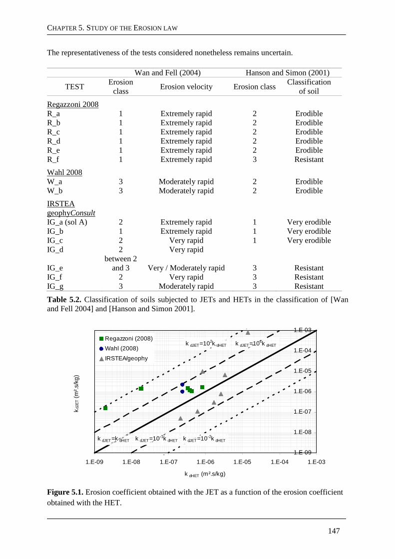
CHAPTER 5. STUDY OF THE EROSION LAW
147
The representativeness of the tests considered nonetheless remains uncertain.
Wan and Fell (2004) Hanson and Simon (2001)
TEST Erosion
class Erosion velocity Erosion class
Classification of soil
Regazzoni 2008 R_a 1 Extremely rapid 2 Erodible R_b 1 Extremely rapid 2 Erodible R_c 1 Extremely rapid 2 Erodible R_d 1 Extremely rapid 2 Erodible R_e 1 Extremely rapid 2 Erodible R_f 1 Extremely rapid 3 Resistant
Wahl 2008 W_a 3 Moderately rapid 2 Erodible W_b 3 Moderately rapid 2 Erodible
IRSTEA geophyConsult IG_a (sol A) 2 Extremely rapid 1 Very erodible IG_b 1 Extremely rapid 1 Very erodible IG_c 2 Very rapid 1 Very erodible IG_d 2 Very rapid
IG_e between 2
and 3 Very / Moderately rapid 3 Resistant IG_f 2 Very rapid 3 Resistant IG_g 3 Moderately rapid 3 Resistant
Table 5.2. Classification of soils subjected to JETs and HETs in the classification of [Wan and Fell 2004] and [Hanson and Simon 2001].
1.E-09
1.E-08
1.E-07
1.E-06
1.E-05
1.E-04
1.E-03
1.E-09 1.E-08 1.E-07 1.E-06 1.E-05 1.E-04 1.E-03
k dHET (m².s/kg)
kdJ
ET (
m².
s/kg
)
Regazzoni (2008)
Wahl (2008)
IRSTEA/geophy
k dJET=k dHET k dJET=10-1k dHET k dJET=10-2k dHET
k dJET=102k dHET k dJET=101k dHET
Figure 5.1. Erosion coefficient obtained with the JET as a function of the erosion coefficient obtained with the HET.
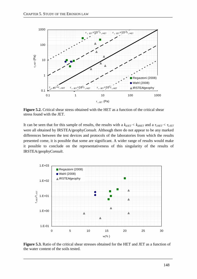
CHAPTER 5. STUDY OF THE EROSION LAW
148
0.1
1
10
100
1000
0.1 1 10 100 1000
τ c JET (Pa)
τcH
ET (
Pa)
Regazzoni (2008)
Wahl (2008)
IRSTEA/geophy
τ c JET=10-2τ cHET
τ c JET=102τ c HETτ c JET=101
τ cHET
τ c JET=10-1τ cHET
τ c JET=τ cHET
Figure 5.2. Critical shear stress obtained with the HET as a function of the critical shear stress found with the JET. It can be seen that for this sample of results, the results with a kdJET < kdHET and a τcHET < τcJET were all obtained by IRSTEA/geophyConsult. Although there do not appear to be any marked differences between the test devices and protocols of the laboratories from which the results presented come, it is possible that some are significant. A wider range of results would make it possible to conclude on the representativeness of this singularity of the results of IRSTEA/geophyConsult.
1.E-01
1.E+00
1.E+01
1.E+02
1.E+03
0 5 10 15 20 25 30
w(% )
τc
HE
T/τc
JE
T
Regazzoni (2008)
Wahl (2008)
IRSTEA/geophy
Figure 5.3. Ratio of the critical shear stresses obtained for the HET and JET as a function of the water content of the soils tested.
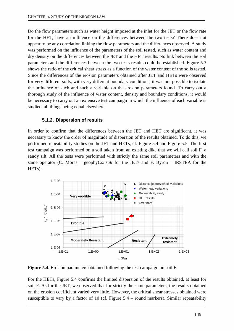
CHAPTER 5. STUDY OF THE EROSION LAW
149
Do the flow parameters such as water height imposed at the inlet for the JET or the flow rate for the HET, have an influence on the differences between the two tests? There does not appear to be any correlation linking the flow parameters and the differences observed. A study was performed on the influence of the parameters of the soil tested, such as water content and dry density on the differences between the JET and the HET results. No link between the soil parameters and the differences between the two tests results could be established. Figure 5.3 shows the ratio of the critical shear stress as a function of the water content of the soils tested. Since the differences of the erosion parameters obtained after JET and HETs were observed for very different soils, with very different boundary conditions, it was not possible to isolate the influence of such and such a variable on the erosion parameters found. To carry out a thorough study of the influence of water content, density and boundary conditions, it would be necessary to carry out an extensive test campaign in which the influence of each variable is studied, all things being equal elsewhere.
5.1.2. Dispersion of results
In order to confirm that the differences between the JET and HET are significant, it was necessary to know the order of magnitude of dispersion of the results obtained. To do this, we performed repeatability studies on the JET and HETs, cf. Figure 5.4 and Figure 5.5. The first test campaign was performed on a soil taken from an existing dike that we will call soil F, a sandy silt. All the tests were performed with strictly the same soil parameters and with the same operator (C. Moras – geophyConsult for the JETs and F. Byron – IRSTEA for the HETs).
1.E-08
1.E-07
1.E-06
1.E-05
1.E-04
1.E-03
1.E-01 1.E+00 1.E+01 1.E+02 1.E+03
k d(m
2 /.s
/kg)
τc (Pa)
Distance jet nozzle/soil variations
Water head variations
Repeatability study
HET results
Error bars
Very erodible
Moderately Resistant ResistantExtremelyresistant
Erodible
Figure 5.4. Erosion parameters obtained following the test campaign on soil F. For the HETs, Figure 5.4 confirms the limited dispersion of the results obtained, at least for soil F. As for the JET, we observed that for strictly the same parameters, the results obtained on the erosion coefficient varied very little. However, the critical shear stresses obtained were susceptible to vary by a factor of 10 (cf. Figure 5.4 – round markers). Similar repeatability
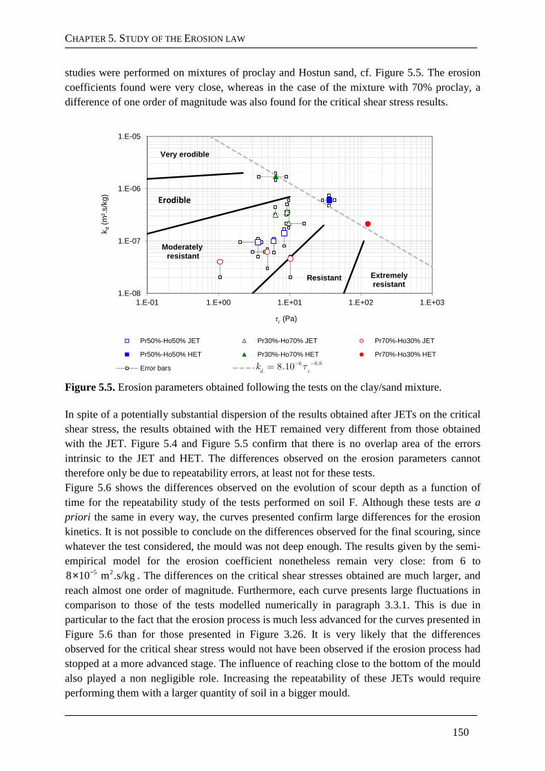
CHAPTER 5. STUDY OF THE EROSION LAW
150
studies were performed on mixtures of proclay and Hostun sand, cf. Figure 5.5. The erosion coefficients found were very close, whereas in the case of the mixture with 70% proclay, a difference of one order of magnitude was also found for the critical shear stress results.
1.E-08
1.E-07
1.E-06
1.E-05
1.E-01 1.E+00 1.E+01 1.E+02 1.E+03
k d(m
².s/
kg)
τc (Pa)
Pr50%-Ho50% JET Pr30%-Ho70% JET Pr70%-Ho30% JET
Pr50%-Ho50% HET Pr30%-Ho70% HET Pr70%-Ho30% HET
Error bars kd=6tauc^-0.8
Very erodible
Moderatelyresistant
Resistant Extremelyresistant
Erodible
6 0 88 10
.
d ck . τ− −
=
Figure 5.5. Erosion parameters obtained following the tests on the clay/sand mixture. In spite of a potentially substantial dispersion of the results obtained after JETs on the critical shear stress, the results obtained with the HET remained very different from those obtained with the JET. Figure 5.4 and Figure 5.5 confirm that there is no overlap area of the errors intrinsic to the JET and HET. The differences observed on the erosion parameters cannot therefore only be due to repeatability errors, at least not for these tests. Figure 5.6 shows the differences observed on the evolution of scour depth as a function of time for the repeatability study of the tests performed on soil F. Although these tests are a priori the same in every way, the curves presented confirm large differences for the erosion kinetics. It is not possible to conclude on the differences observed for the final scouring, since whatever the test considered, the mould was not deep enough. The results given by the semi-empirical model for the erosion coefficient nonetheless remain very close: from 6 to
5 28 10 m .s/kg−× . The differences on the critical shear stresses obtained are much larger, and reach almost one order of magnitude. Furthermore, each curve presents large fluctuations in comparison to those of the tests modelled numerically in paragraph 3.3.1. This is due in particular to the fact that the erosion process is much less advanced for the curves presented in Figure 5.6 than for those presented in Figure 3.26. It is very likely that the differences observed for the critical shear stress would not have been observed if the erosion process had stopped at a more advanced stage. The influence of reaching close to the bottom of the mould also played a non negligible role. Increasing the repeatability of these JETs would require performing them with a larger quantity of soil in a bigger mould.
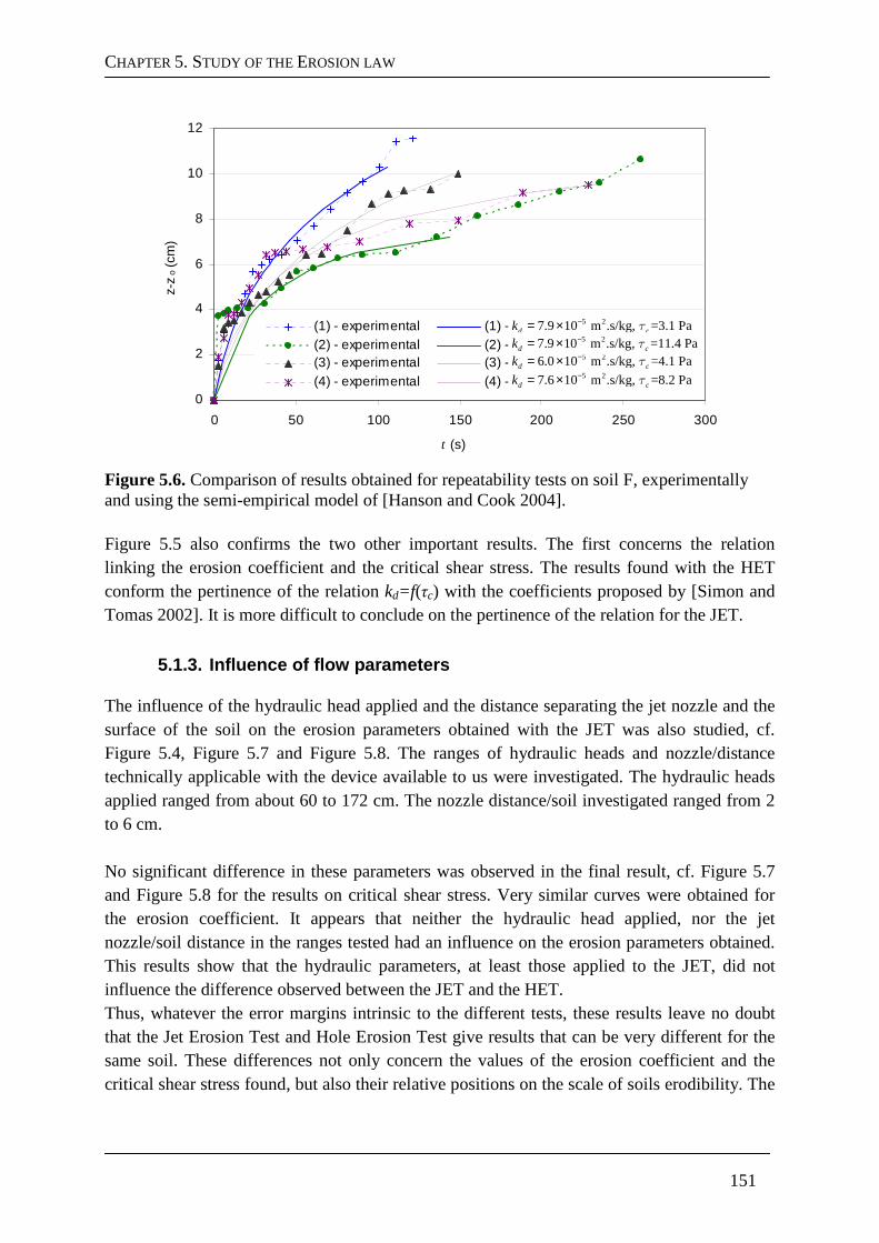
CHAPTER 5. STUDY OF THE EROSION LAW
151
0
2
4
6
8
10
12
0 50 100 150 200 250 300
t (s)
z-z
o (c
m)
(1) - experimental (1) - (2) - experimental (2) - (3) - experimental (3) - (4) - experimental (4) -
5 27.9 10 m .s/kg, =3.1 Pa d ck τ−= ×
5 26.0 10 m .s/kg, =4.1 Pa d ck τ−= ×
5 27.9 10 m .s/kg, =11.4 Pa d ck τ−= ×
5 27.6 10 m .s/kg, =8.2 Pa d ck τ−= ×
Figure 5.6. Comparison of results obtained for repeatability tests on soil F, experimentally and using the semi-empirical model of [Hanson and Cook 2004].
Figure 5.5 also confirms the two other important results. The first concerns the relation linking the erosion coefficient and the critical shear stress. The results found with the HET conform the pertinence of the relation kd=f(τc) with the coefficients proposed by [Simon and Tomas 2002]. It is more difficult to conclude on the pertinence of the relation for the JET.
5.1.3. Influence of flow parameters
The influence of the hydraulic head applied and the distance separating the jet nozzle and the surface of the soil on the erosion parameters obtained with the JET was also studied, cf. Figure 5.4, Figure 5.7 and Figure 5.8. The ranges of hydraulic heads and nozzle/distance technically applicable with the device available to us were investigated. The hydraulic heads applied ranged from about 60 to 172 cm. The nozzle distance/soil investigated ranged from 2 to 6 cm. No significant difference in these parameters was observed in the final result, cf. Figure 5.7 and Figure 5.8 for the results on critical shear stress. Very similar curves were obtained for the erosion coefficient. It appears that neither the hydraulic head applied, nor the jet nozzle/soil distance in the ranges tested had an influence on the erosion parameters obtained. This results show that the hydraulic parameters, at least those applied to the JET, did not influence the difference observed between the JET and the HET. Thus, whatever the error margins intrinsic to the different tests, these results leave no doubt that the Jet Erosion Test and Hole Erosion Test give results that can be very different for the same soil. These differences not only concern the values of the erosion coefficient and the critical shear stress found, but also their relative positions on the scale of soils erodibility. The
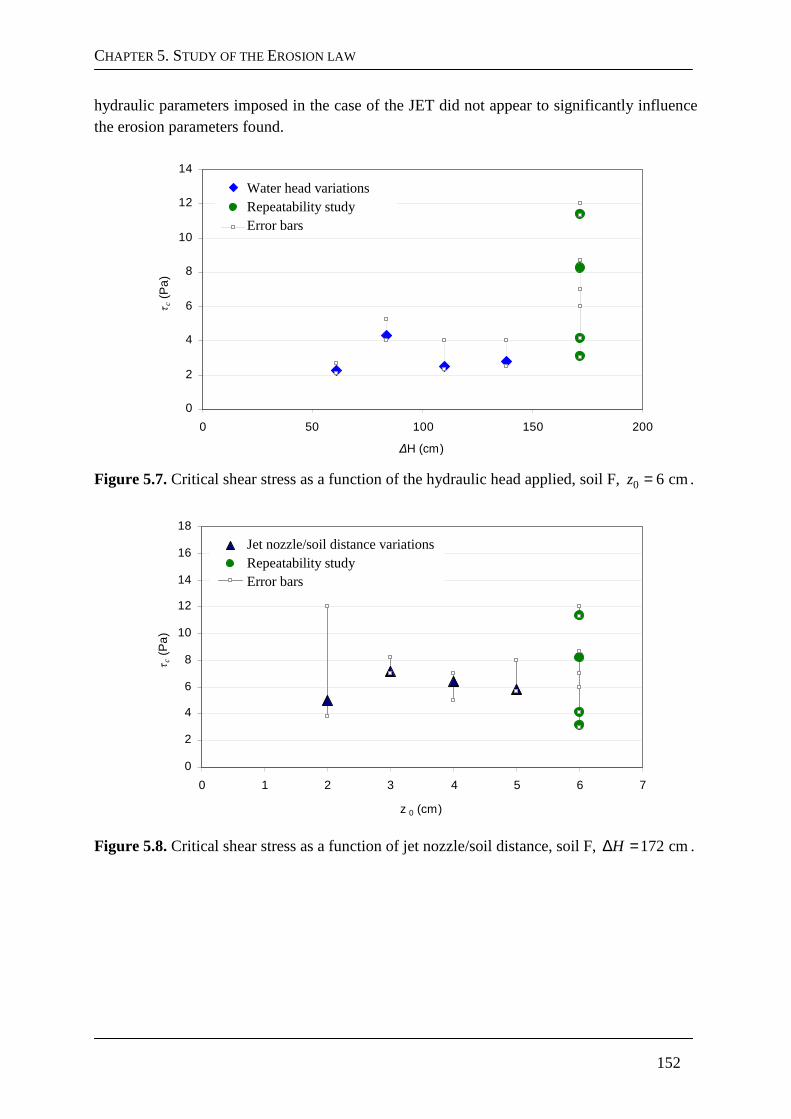
CHAPTER 5. STUDY OF THE EROSION LAW
152
hydraulic parameters imposed in the case of the JET did not appear to significantly influence the erosion parameters found.
0
2
4
6
8
10
12
14
0 50 100 150 200
∆H (cm)
τc
(Pa)
Hauteur d'eau variable
Essais de répétabilité
Barres d'erreur
Figure 5.7. Critical shear stress as a function of the hydraulic head applied, soil F, 0 6 cm=z .
0
2
4
6
8
10
12
14
16
18
0 1 2 3 4 5 6 7
z 0 (cm)
τc
(Pa)
Distance buse matériau variable
Essais de répétabilitéBarres d'erreur
Figure 5.8. Critical shear stress as a function of jet nozzle/soil distance, soil F, 172 cm∆ =H .
Water head variations Repeatability study Error bars
Jet nozzle/soil distance variations Repeatability study Error bars
CHAPTER 5. STUDY OF THE EROSION LAW
153
5.2. Variables susceptible to influence erosion
5.2.1. Possible explanations for JET and HET differences?
The accuracy of the differences on the erosion parameters found for the JET and the HET was validated. How can these differences be explained? The erosion parameters obtained with the interpretation models on the basis of the experimental results, which differ for the JET and the HET, permit obtaining the evolution of the water/soil interface as a function of time following complex CFD modelling. It was deduced that the erosion parameters found did not characterise the same magnitude. Let us try to understand why. The first hypothesis is that the erosion modes governing the detachment of soil particles differ greatly according to the type of hydraulic stress. To our knowledge little research has involved studies of erosion modes. In the framework of a work on the physics of cohesive sediments in a maritime environment, [Winterwerp and Van Kesteren 2004] distinguished three erosion modes: floc erosion, surface erosion and volume erosion. The authors showed that according to the hydraulic head applied, the same soil can be eroded in different modes. The study presented in paragraph 5.1.3 shows that the hydraulic head imposed in the JET had no influence on the erosion parameters. Nonetheless, it is possible that the angle of incidence of the flow led to the solicitation of different erosion modes. This is why a tensoral definition of the erosion law could be a solution. Two couples of
dk and
cτ , relative to erosion under a
tangential and normal flow must be defined. In this hypothesis, the results obtained following the JET and HETs are therefore complementary. An experimental study of erosion modes as a function of angle of incidence would allow concluding as to the validity of this hypothesis. The second hypothesis, which is not incompatible with the first, is that the erosion law is incomplete. We will study this hypothesis in detail in the rest of this chapter. The erosion parameters are adjustment parameters of the erosion law. These parameters are adjusted so that the curve of erosion rate versus the shear stress obtained by the model fits the experimental results as well as possible, cf. Figure 5.9. It is probable that taking other flow variables and parameters into account may allow grouping the erosion rate curves obtained with the JET and HET. The erosion parameters obtained in this way would therefore be intrinsic to the soil. Another possibility would be to develop erosion parameters obtained as a function of soil characteristics and flow parameters. Furthermore, apart from the variables relating to flow in the erosion law, the simplifications relating to the maximum stress in the JET interpretation model remain problematic. The shear stress used in the two interpretation models as a function of erosion time do not depend on the position of the region to be eroded on the water/soil interface. The shear stress is almost constant along the whole interface in the case of the HET, excluding the geometric singularities. However, this is not the case for the JET. It is necessary to adjust the erosion law Eq. (2.20) to obtain results in good agreement with the experimental results. The shape of the erosion figure obtained numerically corresponds well with that obtained experimentally. This means that, at least in terms of orders of magnitude, the erosion parameters are not or
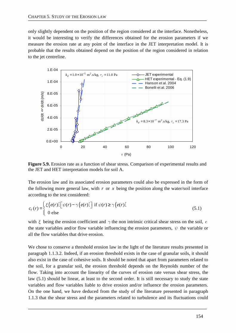
CHAPTER 5. STUDY OF THE EROSION LAW
154
only slightly dependent on the position of the region considered at the interface. Nonetheless, it would be interesting to verify the differences obtained for the erosion parameters if we measure the erosion rate at any point of the interface in the JET interpretation model. It is probable that the results obtained depend on the position of the region considered in relation to the jet centreline.
0.E+00
2.E-05
4.E-05
6.E-05
8.E-05
1.E-04
1.E-04
0 20 40 60 80 100 120
τ (Pa)
dz/
dt o
u d
r/dt (
m/s
)
JET experimentalHET experimental - Eq. (1.9)Hanson et al. 2004Bonelli et al. 2006
5 21.0 10 m .s/kg, 11.0 Pad ck τ−= × =
7 28.3 10 m .s/kg, 17.3 Pad ck τ−= × =
Figure 5.9. Erosion rate as a function of shear stress. Comparison of experimental results and the JET and HET interpretation models for soil A. The erosion law and its associated erosion parameters could also be expressed in the form of the following more general law, with r or x being the position along the water/soil interface according to the test considered:
( ) ( ) ( )( ) ( ) ( ) if ( ) ( )( )
0 else
e r r e r r e rc rΓ
− ≥ =
ξ ψ γ ψ γ (5.1)
with ξ being the erosion coefficient and γ the non intrinsic critical shear stress on the soil, e the state variables and/or flow variable influencing the erosion parameters, ψ the variable or all the flow variables that drive erosion. We chose to conserve a threshold erosion law in the light of the literature results presented in paragraph 1.1.3.2. Indeed, if an erosion threshold exists in the case of granular soils, it should also exist in the case of cohesive soils. It should be noted that apart from parameters related to the soil, for a granular soil, the erosion threshold depends on the Reynolds number of the flow. Taking into account the linearity of the curves of erosion rate versus shear stress, the law (5.1) should be linear, at least to the second order. It is still necessary to study the state variables and flow variables liable to drive erosion and/or influence the erosion parameters. On the one hand, we have deduced from the study of the literature presented in paragraph 1.1.3 that the shear stress and the parameters related to turbulence and its fluctuations could
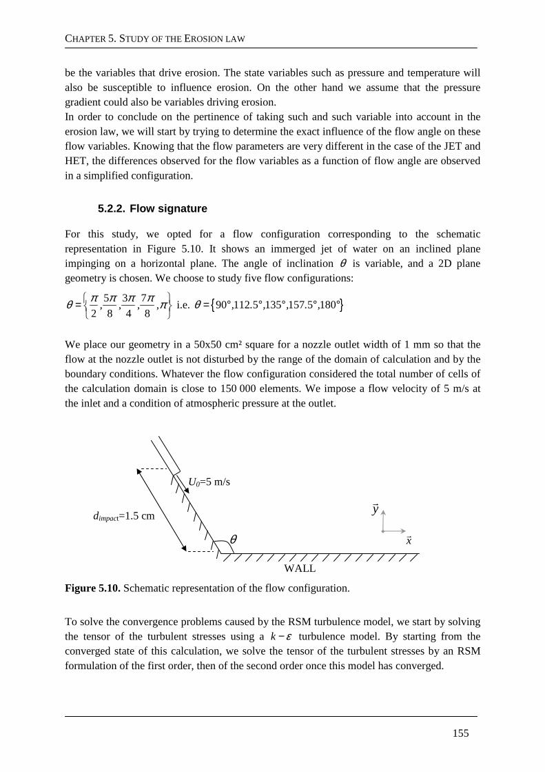
CHAPTER 5. STUDY OF THE EROSION LAW
155
be the variables that drive erosion. The state variables such as pressure and temperature will also be susceptible to influence erosion. On the other hand we assume that the pressure gradient could also be variables driving erosion. In order to conclude on the pertinence of taking such and such variable into account in the erosion law, we will start by trying to determine the exact influence of the flow angle on these flow variables. Knowing that the flow parameters are very different in the case of the JET and HET, the differences observed for the flow variables as a function of flow angle are observed in a simplified configuration.
5.2.2. Flow signature
For this study, we opted for a flow configuration corresponding to the schematic representation in Figure 5.10. It shows an immerged jet of water on an inclined plane impinging on a horizontal plane. The angle of inclination θ is variable, and a 2D plane geometry is chosen. We choose to study five flow configurations:
5 3 7
2 8 4 8, , , ,
π π π πθ π =
i.e. 90 112 5 135 157 5 180, . , , . ,θ = ° ° ° ° °
We place our geometry in a 50x50 cm² square for a nozzle outlet width of 1 mm so that the flow at the nozzle outlet is not disturbed by the range of the domain of calculation and by the boundary conditions. Whatever the flow configuration considered the total number of cells of the calculation domain is close to 150 000 elements. We impose a flow velocity of 5 m/s at the inlet and a condition of atmospheric pressure at the outlet.
Figure 5.10. Schematic representation of the flow configuration.
To solve the convergence problems caused by the RSM turbulence model, we start by solving the tensor of the turbulent stresses using a k ε− turbulence model. By starting from the converged state of this calculation, we solve the tensor of the turbulent stresses by an RSM formulation of the first order, then of the second order once this model has converged.
x
y
WALL
θ
dimpact=1.5 cm
U0=5 m/s
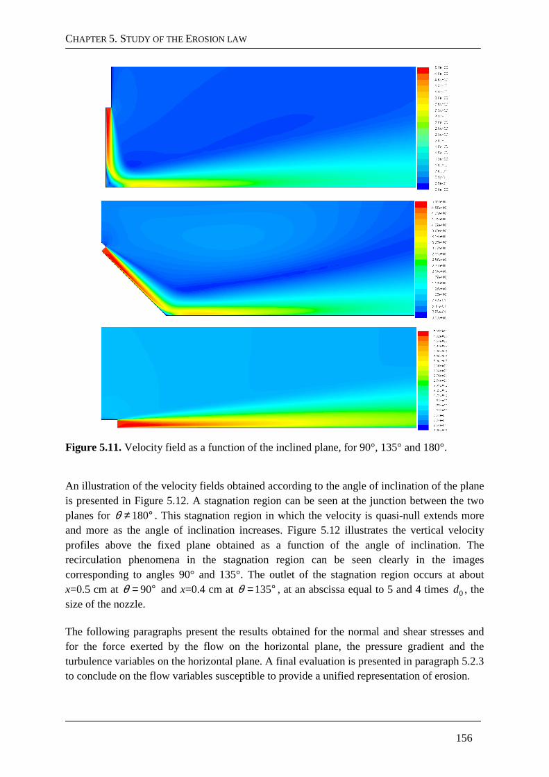
CHAPTER 5. STUDY OF THE EROSION LAW
156
Figure 5.11. Velocity field as a function of the inclined plane, for 90°, 135° and 180°.
An illustration of the velocity fields obtained according to the angle of inclination of the plane is presented in Figure 5.12. A stagnation region can be seen at the junction between the two planes for 180θ ≠ ° . This stagnation region in which the velocity is quasi-null extends more and more as the angle of inclination increases. Figure 5.12 illustrates the vertical velocity profiles above the fixed plane obtained as a function of the angle of inclination. The recirculation phenomena in the stagnation region can be seen clearly in the images corresponding to angles 90° and 135°. The outlet of the stagnation region occurs at about x=0.5 cm at 90θ = ° and x=0.4 cm at 135θ = ° , at an abscissa equal to 5 and 4 times 0d , the size of the nozzle. The following paragraphs present the results obtained for the normal and shear stresses and for the force exerted by the flow on the horizontal plane, the pressure gradient and the turbulence variables on the horizontal plane. A final evaluation is presented in paragraph 5.2.3 to conclude on the flow variables susceptible to provide a unified representation of erosion.
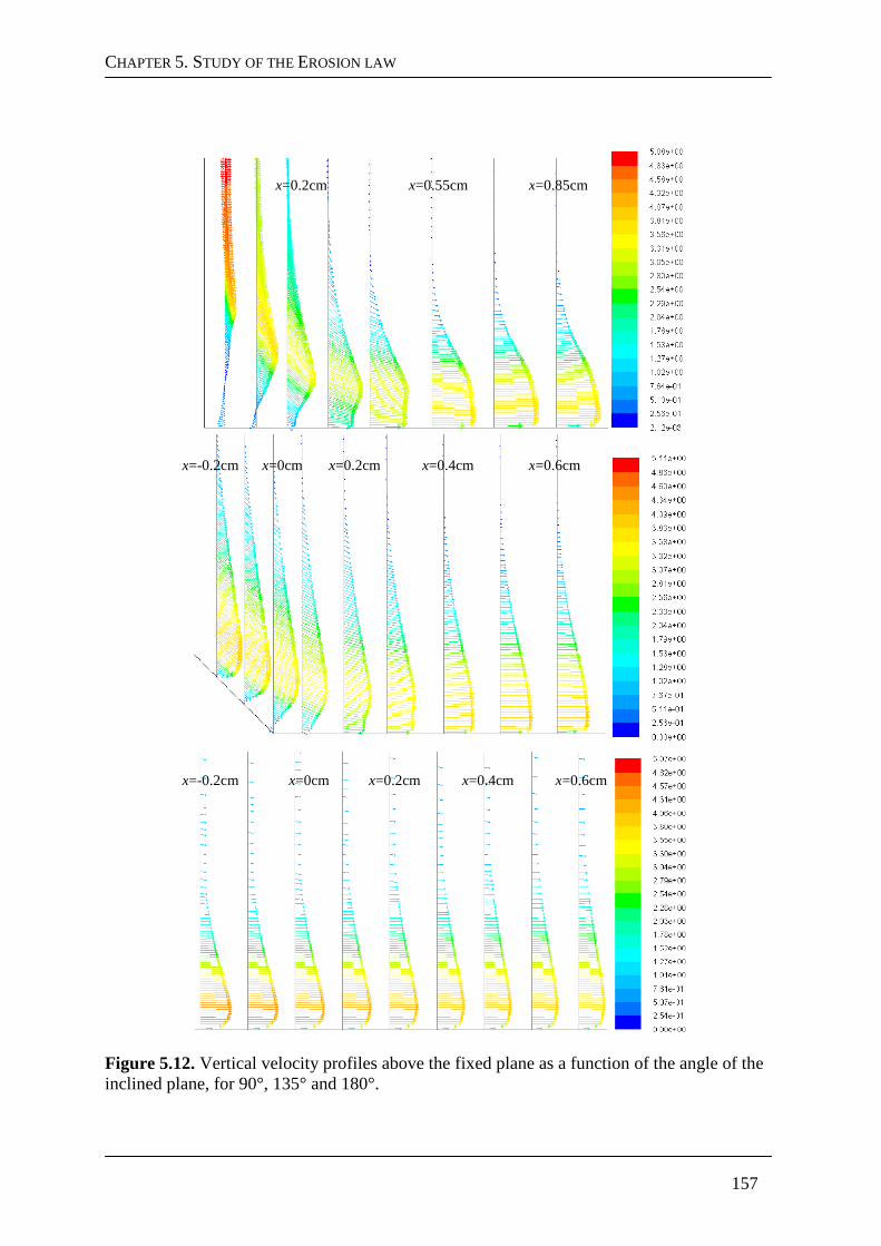
CHAPTER 5. STUDY OF THE EROSION LAW
157
Figure 5.12. Vertical velocity profiles above the fixed plane as a function of the angle of the inclined plane, for 90°, 135° and 180°.
x=0.55cm x=0.85cm x=0.2cm
x=0.4cm x=0.6cm x=0.2cm x=0cm x=-0.2cm
x=0.4cm x=0.6cm x=0.2cm x=0cm x=-0.2cm
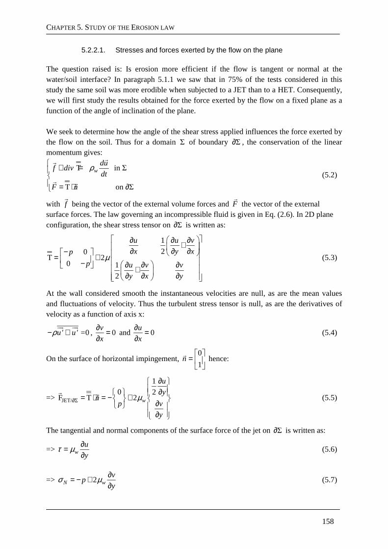
CHAPTER 5. STUDY OF THE EROSION LAW
158
5.2.2.1. Stresses and forces exerted by the flow on the plane The question raised is: Is erosion more efficient if the flow is tangent or normal at the water/soil interface? In paragraph 5.1.1 we saw that in 75% of the tests considered in this study the same soil was more erodible when subjected to a JET than to a HET. Consequently, we will first study the results obtained for the force exerted by the flow on a fixed plane as a function of the angle of inclination of the plane. We seek to determine how the angle of the shear stress applied influences the force exerted by the flow on the soil. Thus for a domain Σ of boundary Σ∂ , the conservation of the linear momentum gives:
T in Σ
T on Σ
wdu
f divdt
F n
ρ + = = ⋅ ∂
(5.2)
with f
being the vector of the external volume forces and F
the vector of the external surface forces. The law governing an incompressible fluid is given in Eq. (2.6). In 2D plane configuration, the shear stress tensor on Σ∂ is written as:
1
20T 2
0 1
2
µ
∂ ∂ ∂+ ∂ ∂ ∂− = + − ∂ ∂ ∂ + ∂ ∂ ∂
u u v
x y xp
p u v v
y x y
(5.3)
At the wall considered smooth the instantaneous velocities are null, as are the mean values and fluctuations of velocity. Thus the turbulent stress tensor is null, as are the derivatives of velocity as a function of axis x:
=0u' u'ρ− ⊗
, 0v
x
∂ =∂
and 0u
x
∂ =∂
(5.4)
On the surface of horizontal impingement, 0
1n
=
hence:
=> JET/ Σ
10 2
F T 2 w
u
yn
p v
y
∂
∂ ∂ = ⋅ = − + ∂ ∂
µ (5.5)
The tangential and normal components of the surface force of the jet on Σ∂ is written as:
=> wu
y
∂=∂
τ µ (5.6)
=> 2N wv
py
∂= − +∂
σ µ (5.7)
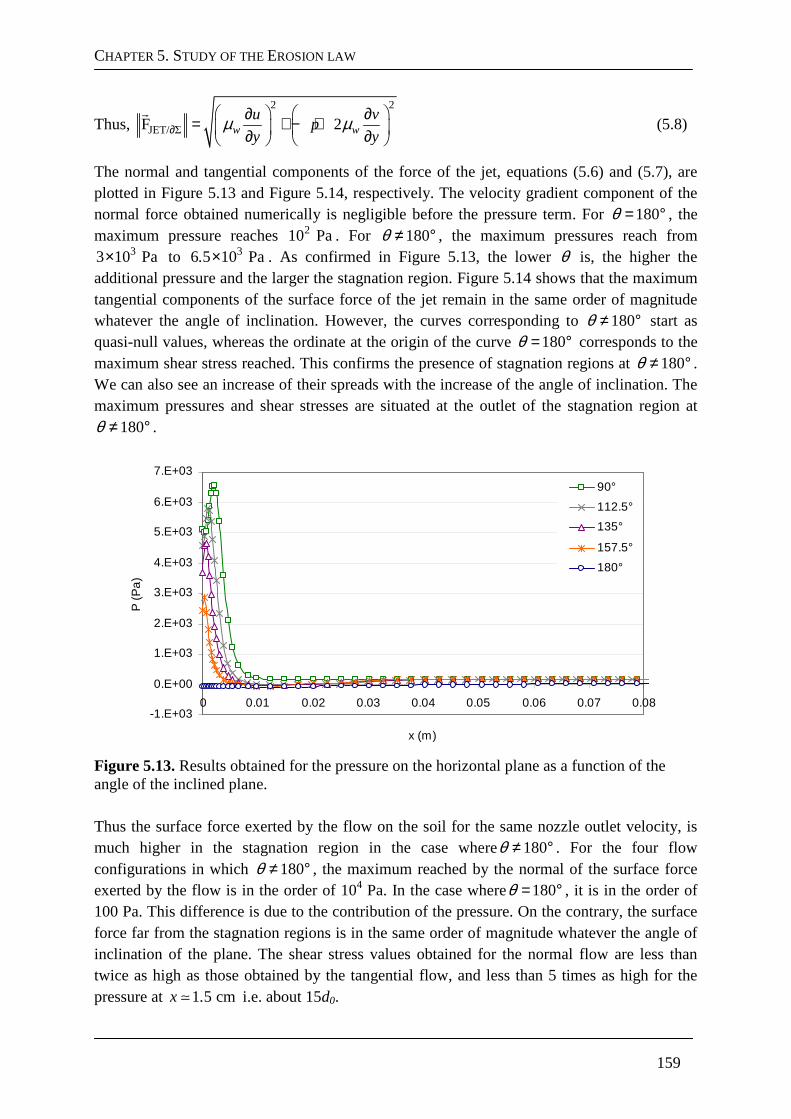
CHAPTER 5. STUDY OF THE EROSION LAW
159
Thus, 2 2
JET/ ΣF 2w wu v
py y∂
∂ ∂= + − + ∂ ∂
µ µ (5.8)
The normal and tangential components of the force of the jet, equations (5.6) and (5.7), are plotted in Figure 5.13 and Figure 5.14, respectively. The velocity gradient component of the normal force obtained numerically is negligible before the pressure term. For 180θ = ° , the maximum pressure reaches 210 Pa. For 180θ ≠ ° , the maximum pressures reach from
33 10 Pa× to 36 5 10 Pa. × . As confirmed in Figure 5.13, the lower θ is, the higher the additional pressure and the larger the stagnation region. Figure 5.14 shows that the maximum tangential components of the surface force of the jet remain in the same order of magnitude whatever the angle of inclination. However, the curves corresponding to 180θ ≠ ° start as quasi-null values, whereas the ordinate at the origin of the curve 180θ = ° corresponds to the maximum shear stress reached. This confirms the presence of stagnation regions at 180θ ≠ ° . We can also see an increase of their spreads with the increase of the angle of inclination. The maximum pressures and shear stresses are situated at the outlet of the stagnation region at
180θ ≠ ° .
-1.E+03
0.E+00
1.E+03
2.E+03
3.E+03
4.E+03
5.E+03
6.E+03
7.E+03
0 0.01 0.02 0.03 0.04 0.05 0.06 0.07 0.08
x (m)
P (P
a)
90°
112.5°
135°
157.5°
180°
Figure 5.13. Results obtained for the pressure on the horizontal plane as a function of the angle of the inclined plane. Thus the surface force exerted by the flow on the soil for the same nozzle outlet velocity, is much higher in the stagnation region in the case where 180θ ≠ ° . For the four flow configurations in which 180θ ≠ ° , the maximum reached by the normal of the surface force exerted by the flow is in the order of 104 Pa. In the case where 180θ = ° , it is in the order of 100 Pa. This difference is due to the contribution of the pressure. On the contrary, the surface force far from the stagnation regions is in the same order of magnitude whatever the angle of inclination of the plane. The shear stress values obtained for the normal flow are less than twice as high as those obtained by the tangential flow, and less than 5 times as high for the pressure at 1 5 cmx .≃ i.e. about 15d0.
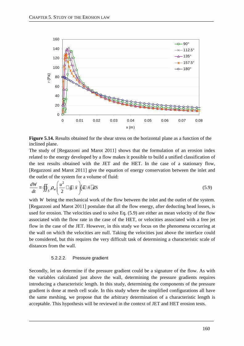
CHAPTER 5. STUDY OF THE EROSION LAW
160
0
20
40
60
80
100
120
140
160
0 0.01 0.02 0.03 0.04 0.05 0.06 0.07 0.08
x (m)
τ (P
a)
90°
112.5°
135°
157.5°
180°
Figure 5.14. Results obtained for the shear stress on the horizontal plane as a function of the inclined plane. The study of [Regazzoni and Marot 2011] shows that the formulation of an erosion index related to the energy developed by a flow makes it possible to build a unified classification of the test results obtained with the JET and the HET. In the case of a stationary flow, [Regazzoni and Marot 2011] give the equation of energy conservation between the inlet and the outlet of the system for a volume of fluid:
( )2
2wS
dW ug x u n dS
dt
= + ⋅ ⋅
∫∫
ρ (5.9)
with W being the mechanical work of the flow between the inlet and the outlet of the system. [Regazzoni and Marot 2011] postulate that all the flow energy, after deducting head losses, is used for erosion. The velocities used to solve Eq. (5.9) are either an mean velocity of the flow associated with the flow rate in the case of the HET, or velocities associated with a free jet flow in the case of the JET. However, in this study we focus on the phenomena occurring at the wall on which the velocities are null. Taking the velocities just above the interface could be considered, but this requires the very difficult task of determining a characteristic scale of distances from the wall.
5.2.2.2. Pressure gradient Secondly, let us determine if the pressure gradient could be a signature of the flow. As with the variables calculated just above the wall, determining the pressure gradients requires introducing a characteristic length. In this study, determining the components of the pressure gradient is done at mesh cell scale. In this study where the simplified configurations all have the same meshing, we propose that the arbitrary determination of a characteristic length is acceptable. This hypothesis will be reviewed in the context of JET and HET erosion tests.
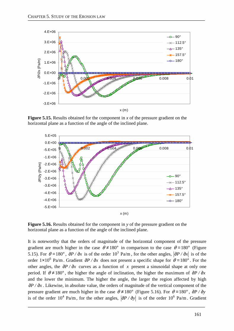
CHAPTER 5. STUDY OF THE EROSION LAW
161
-3.E+06
-2.E+06
-1.E+06
0.E+00
1.E+06
2.E+06
3.E+06
4.E+06
0 0.002 0.004 0.006 0.008 0.01
x (m)
∂P
/∂x
(Pa/
m)
90°
112.5°
135°
157.5°
180°
Figure 5.15. Results obtained for the component in x of the pressure gradient on the horizontal plane as a function of the angle of the inclined plane.
-5.E+06
-4.E+06
-4.E+06
-3.E+06
-3.E+06
-2.E+06
-2.E+06
-1.E+06
-5.E+05
0.E+00
5.E+05
0 0.002 0.004 0.006 0.008 0.01
x (m)
∂P
/∂y
(Pa/
m)
90°
112.5°
135°
157.5°
180°
Figure 5.16. Results obtained for the component in y of the pressure gradient on the horizontal plane as a function of the angle of the inclined plane. It is noteworthy that the orders of magnitude of the horizontal component of the pressure gradient are much higher in the case 180θ ≠ ° in comparison to the case 180θ = ° (Figure 5.15). For 180θ = ° , ∂ ∂P / x is of the order 310 Pa/m, for the other angles, ∂ ∂P / x is of the order 61 10 Pa/m× . Gradient ∂ ∂P / x does not present a specific shape for 180θ = ° . For the other angles, the ∂ ∂P / x curves as a function of x present a sinusoidal shape at only one period. If 180θ ≠ ° , the higher the angle of inclination, the higher the maximum of ∂ ∂P / x and the lower the minimum. The higher the angle, the larger the region affected by high ∂ ∂P / x . Likewise, in absolute value, the orders of magnitude of the vertical component of the pressure gradient are much higher in the case 180θ ≠ ° (Figure 5.16). For 180θ = ° , ∂ ∂P / y is of the order 410 Pa/m, for the other angles, ∂ ∂P / y is of the order 610 Pa/m. Gradient
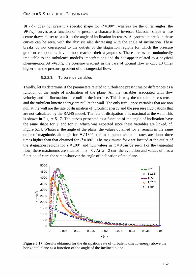
CHAPTER 5. STUDY OF THE EROSION LAW
162
∂ ∂P / y does not present a specific shape for 180θ = ° , whereas for the other angles, the ∂ ∂P / y curves as a function of x present a characteristic inversed Gaussian shape whose centre draws closer to 0=x as the angle of inclination increases. A systematic break in these curves can be seen, with the abscissa also decreasing with the angle of inclination. These breaks do not correspond to the outlets of the stagnation regions for which the pressure gradient components have almost reached their asymptotes. These breaks are undoubtedly imputable to the turbulence model’s imperfections and do not appear related to a physical phenomenon. At x≈20d0, the pressure gradient in the case of normal flow is only 10 times higher than the pressure gradient of the tangential flow.
5.2.2.3. Turbulence variables Thirdly, let us determine if the parameters related to turbulence present major differences as a function of the angle of inclination of the plane. All the variables associated with flow velocity and its fluctuations are null at the interface. This is why the turbulent stress tensor and the turbulent kinetic energy are null at the wall. The only turbulence variables that are non null at the wall are the rate of dissipation of turbulent energy and the pressure fluctuations that are not calculated by the RANS model. The rate of dissipation ε is maximal at the wall. This is shown in Figure 5.17. The curves presented as a function of the angle of inclination have the same shape for ε and for τ , which was expected since these variables are linked, cf. Figure 5.14. Whatever the angle of the plane, the values obtained for ε remain in the same order of magnitude, although for 180θ ≠ ° , the maximum dissipation rates are about three times higher than that obtained for 180= °θ . The maximums for ε are located at the outlet of the stagnation regions for 180θ ≠ ° and null values in 0=x can be seen. For the tangential flow, these maximums are situated in 0=x . At 2 cmx = , the evolution and values of ε as a function of x are the same whatever the angle of inclination of the plane.
0
500
1000
1500
2000
2500
3000
3500
4000
4500
5000
0 0.005 0.01 0.015 0.02 0.025 0.03 0.035 0.04
x (m)
ε (
m²/
s3 )
90°
112.5°
135°157.5°
180°
Figure 5.17. Results obtained for the dissipation rate of turbulent kinetic energy above the horizontal plane as a function of the angle of the inclined plane.
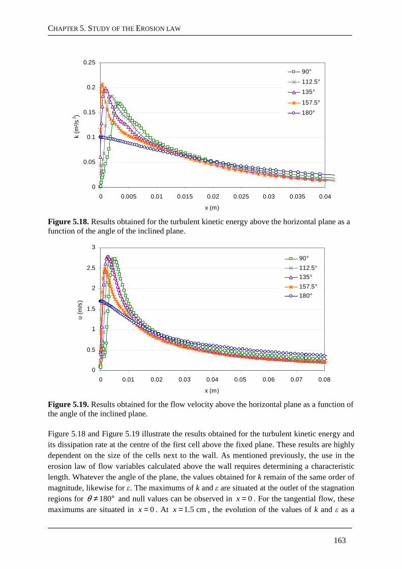
CHAPTER 5. STUDY OF THE EROSION LAW
163
0
0.05
0.1
0.15
0.2
0.25
0 0.005 0.01 0.015 0.02 0.025 0.03 0.035 0.04
x (m)
k (m
²/s
2 )90°
112.5°
135°
157.5°
180°
Figure 5.18. Results obtained for the turbulent kinetic energy above the horizontal plane as a function of the angle of the inclined plane.
0
0.5
1
1.5
2
2.5
3
0 0.01 0.02 0.03 0.04 0.05 0.06 0.07 0.08
x (m)
u (
m/s
)
90°
112.5°
135°
157.5°
180°
Figure 5.19. Results obtained for the flow velocity above the horizontal plane as a function of the angle of the inclined plane. Figure 5.18 and Figure 5.19 illustrate the results obtained for the turbulent kinetic energy and its dissipation rate at the centre of the first cell above the fixed plane. These results are highly dependent on the size of the cells next to the wall. As mentioned previously, the use in the erosion law of flow variables calculated above the wall requires determining a characteristic length. Whatever the angle of the plane, the values obtained for k remain of the same order of magnitude, likewise for ε. The maximums of k and ε are situated at the outlet of the stagnation regions for 180θ ≠ ° and null values can be observed in 0=x . For the tangential flow, these maximums are situated in 0=x . At 1 5 cmx .= , the evolution of the values of k and ε as a
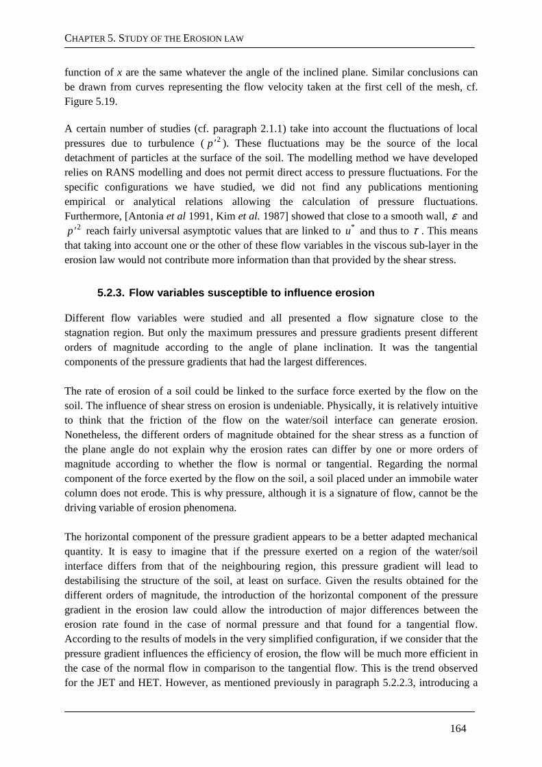
CHAPTER 5. STUDY OF THE EROSION LAW
164
function of x are the same whatever the angle of the inclined plane. Similar conclusions can be drawn from curves representing the flow velocity taken at the first cell of the mesh, cf. Figure 5.19. A certain number of studies (cf. paragraph 2.1.1) take into account the fluctuations of local pressures due to turbulence (2p' ). These fluctuations may be the source of the local detachment of particles at the surface of the soil. The modelling method we have developed relies on RANS modelling and does not permit direct access to pressure fluctuations. For the specific configurations we have studied, we did not find any publications mentioning empirical or analytical relations allowing the calculation of pressure fluctuations. Furthermore, [Antonia et al 1991, Kim et al. 1987] showed that close to a smooth wall, ε and
2p' reach fairly universal asymptotic values that are linked to *u and thus to τ . This means that taking into account one or the other of these flow variables in the viscous sub-layer in the erosion law would not contribute more information than that provided by the shear stress.
5.2.3. Flow variables susceptible to influence eros ion
Different flow variables were studied and all presented a flow signature close to the stagnation region. But only the maximum pressures and pressure gradients present different orders of magnitude according to the angle of plane inclination. It was the tangential components of the pressure gradients that had the largest differences. The rate of erosion of a soil could be linked to the surface force exerted by the flow on the soil. The influence of shear stress on erosion is undeniable. Physically, it is relatively intuitive to think that the friction of the flow on the water/soil interface can generate erosion. Nonetheless, the different orders of magnitude obtained for the shear stress as a function of the plane angle do not explain why the erosion rates can differ by one or more orders of magnitude according to whether the flow is normal or tangential. Regarding the normal component of the force exerted by the flow on the soil, a soil placed under an immobile water column does not erode. This is why pressure, although it is a signature of flow, cannot be the driving variable of erosion phenomena. The horizontal component of the pressure gradient appears to be a better adapted mechanical quantity. It is easy to imagine that if the pressure exerted on a region of the water/soil interface differs from that of the neighbouring region, this pressure gradient will lead to destabilising the structure of the soil, at least on surface. Given the results obtained for the different orders of magnitude, the introduction of the horizontal component of the pressure gradient in the erosion law could allow the introduction of major differences between the erosion rate found in the case of normal pressure and that found for a tangential flow. According to the results of models in the very simplified configuration, if we consider that the pressure gradient influences the efficiency of erosion, the flow will be much more efficient in the case of the normal flow in comparison to the tangential flow. This is the trend observed for the JET and HET. However, as mentioned previously in paragraph 5.2.2.3, introducing a
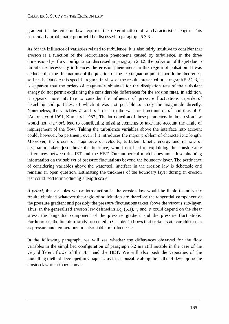
CHAPTER 5. STUDY OF THE EROSION LAW
165
gradient in the erosion law requires the determination of a characteristic length. This particularly problematic point will be discussed in paragraph 5.3.3. As for the influence of variables related to turbulence, it is also fairly intuitive to consider that erosion is a function of the recirculation phenomena caused by turbulence. In the three dimensional jet flow configuration discussed in paragraph 2.3.2, the pulsation of the jet due to turbulence necessarily influences the erosion phenomena in this region of pulsation. It was deduced that the fluctuations of the position of the jet stagnation point smooth the theoretical soil peak. Outside this specific region, in view of the results presented in paragraph 5.2.2.3, it is apparent that the orders of magnitude obtained for the dissipation rate of the turbulent energy do not permit explaining the considerable differences for the erosion rates. In addition, it appears more intuitive to consider the influence of pressure fluctuations capable of detaching soil particles, of which it was not possible to study the magnitude directly. Nonetheless, the variables ε and 2p' close to the wall are functions of *u and thus of τ [Antonia et al 1991, Kim et al. 1987]. The introduction of these parameters in the erosion law would not, a priori, lead to contributing missing elements to take into account the angle of impingement of the flow. Taking the turbulence variables above the interface into account could, however, be pertinent, even if it introduces the major problem of characteristic length. Moreover, the orders of magnitude of velocity, turbulent kinetic energy and its rate of dissipation taken just above the interface, would not lead to explaining the considerable differences between the JET and the HET. Our numerical model does not allow obtaining information on the subject of pressure fluctuations beyond the boundary layer. The pertinence of considering variables above the water/soil interface in the erosion law is debatable and remains an open question. Estimating the thickness of the boundary layer during an erosion test could lead to introducing a length scale. A priori, the variables whose introduction in the erosion law would be liable to unify the results obtained whatever the angle of solicitation are therefore the tangential component of the pressure gradient and possibly the pressure fluctuations taken above the viscous sub-layer. Thus, in the generalised erosion law defined in Eq. (5.1), ψ and e could depend on the shear stress, the tangential component of the pressure gradient and the pressure fluctuations. Furthermore, the literature study presented in Chapter 1 shows that certain state variables such as pressure and temperature are also liable to influence e. In the following paragraph, we will see whether the differences observed for the flow variables in the simplified configuration of paragraph 5.2 are still notable in the case of the very different flows of the JET and the HET. We will also push the capacities of the modelling method developed in Chapter 2 as far as possible along the paths of developing the erosion law mentioned above.
CHAPTER 5. STUDY OF THE EROSION LAW
166
5.3. Paths for developing the erosion law
5.3.1. Flow variables of the JET and HETs
In this study we rely on the case of the JET and HETs carried out on soil A, whose numerical models are presented in Chapters 3 and 4, respectively. In the configuration of the tests carried out on soil A, we have R0=3 mm, L=12 cm, z0=14.6 cm, the radius of the soil sample for the JET rmax=5.6 cm. The pressure differential imposed between the inlet and the outlet of the experimental JET device was 30 000 Pa and the inlet flow rate of the HET was 0.53 m3/h for an output pressure equal to atmospheric pressure.
Figure 5.20. Velocity fields above the water/soil interface at t = 0 s obtained for modelling the JET performed on soil A, with the k ω− model.
Figure 5.20 and Figure 5.21 show the shape of the velocity profiles obtained above the water/soil interface with the models of the JET performed on soil A. In conformity with the graph shown in Figure 3.13, Figure 5.20 illustrates that at t = 0 s, the outlet of the stagnation region of the jet occurs at 1.3 cmr ≃ i.e. at about 02 d× . For more advanced times, the region in which the flow is no longer disturbed by recirculations due to the stagnation point is more difficult to visualise given the curvature of the interface. The outlet of the jet stagnation region nonetheless still appears to correspond well with the minimum radius for which the shear stress appears maximal. In conformity with the results presented in Figure 3.13, at the end of the erosion process, the outlet of the jet stagnation region is close to 9 mmr ≃ . The velocity profiles obtained in the framework of the model of the HET on soil A at the beginning and end of the erosion process are presented in Figure 5.22. The flow establishment length is longer at the end of the erosion process. This is explained by the increase in diameter of the pipe and above all in its upstream part. At t = 0 s, the establishment length is equal to almost 10 times the pipe diameter. At the end of the erosion process it reaches nearly 030 R× . The comparative results of the two tests at 0 st = are presented in Figure 5.23 and Figure 5.24 for the shear stress and the pressure field on the water/soil interface without erosion, respectively. The maximum shear stress is close to max 40 Paτ ≃ for the JET at r/rmax≈0.2. The shear stress remains almost constant for the HET along the water/soil interface, with an
r=2 cm r=3 cm r=4 cm r=1 cm r=0 cm r=5 cm
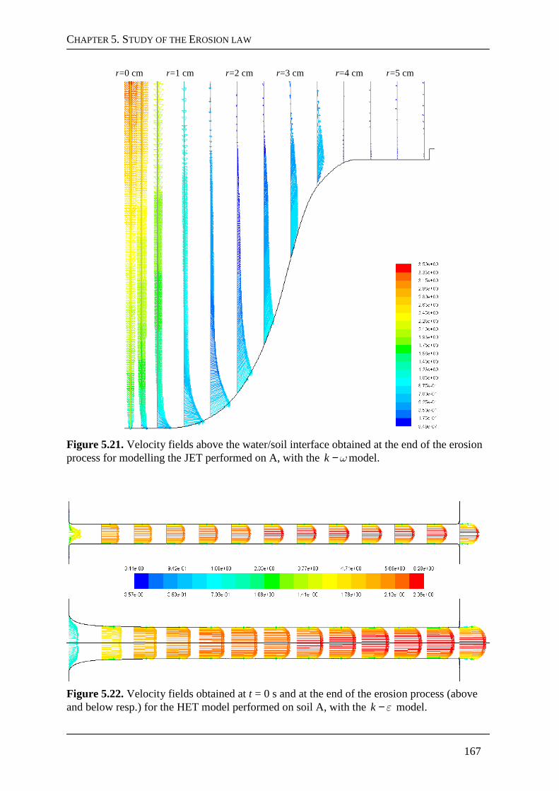
CHAPTER 5. STUDY OF THE EROSION LAW
167
Figure 5.21. Velocity fields above the water/soil interface obtained at the end of the erosion process for modelling the JET performed on A, with the k ω− model.
Figure 5.22. Velocity fields obtained at t = 0 s and at the end of the erosion process (above and below resp.) for the HET model performed on soil A, with the k ε− model.
r=2 cm r=3 cm r=4 cm r=1 cm r=0 cm r=5 cm
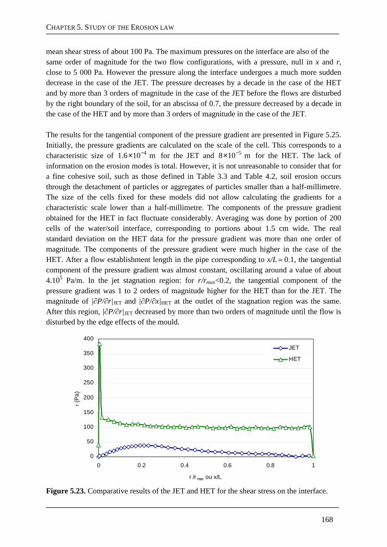
CHAPTER 5. STUDY OF THE EROSION LAW
168
mean shear stress of about 100 Pa. The maximum pressures on the interface are also of the same order of magnitude for the two flow configurations, with a pressure, null in x and r, close to 5 000 Pa. However the pressure along the interface undergoes a much more sudden decrease in the case of the JET. The pressure decreases by a decade in the case of the HET and by more than 3 orders of magnitude in the case of the JET before the flows are disturbed by the right boundary of the soil, for an abscissa of 0.7, the pressure decreased by a decade in the case of the HET and by more than 3 orders of magnitude in the case of the JET. The results for the tangential component of the pressure gradient are presented in Figure 5.25. Initially, the pressure gradients are calculated on the scale of the cell. This corresponds to a characteristic size of 41.6 10 m−× for the JET and 58 10 m−× for the HET. The lack of information on the erosion modes is total. However, it is not unreasonable to consider that for a fine cohesive soil, such as those defined in Table 3.3 and Table 4.2, soil erosion occurs through the detachment of particles or aggregates of particles smaller than a half-millimetre. The size of the cells fixed for these models did not allow calculating the gradients for a characteristic scale lower than a half-millimetre. The components of the pressure gradient obtained for the HET in fact fluctuate considerably. Averaging was done by portion of 200 cells of the water/soil interface, corresponding to portions about 1.5 cm wide. The real standard deviation on the HET data for the pressure gradient was more than one order of magnitude. The components of the pressure gradient were much higher in the case of the HET. After a flow establishment length in the pipe corresponding to x/L≃ 0.1, the tangential component of the pressure gradient was almost constant, oscillating around a value of about 4.105 Pa/m. In the jet stagnation region: for r/rmax<0.2, the tangential component of the pressure gradient was 1 to 2 orders of magnitude higher for the HET than for the JET. The magnitude of |∂P/∂r|JET and |∂P/∂x|HET at the outlet of the stagnation region was the same. After this region, |∂P/∂r|JET decreased by more than two orders of magnitude until the flow is disturbed by the edge effects of the mould.
0
50
100
150
200
250
300
350
400
0 0.2 0.4 0.6 0.8 1
r /r max ou x/L
τ (P
a)
JET
HET
Figure 5.23. Comparative results of the JET and HET for the shear stress on the interface.
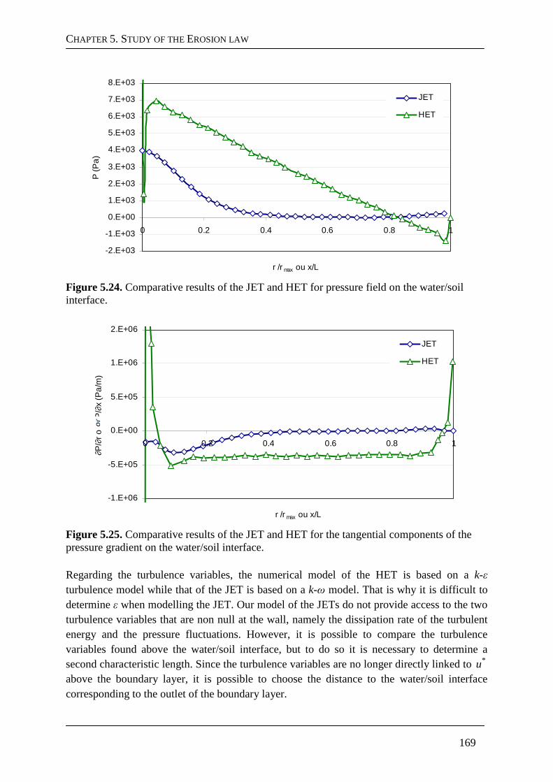
CHAPTER 5. STUDY OF THE EROSION LAW
169
-2.E+03
-1.E+03
0.E+00
1.E+03
2.E+03
3.E+03
4.E+03
5.E+03
6.E+03
7.E+03
8.E+03
0 0.2 0.4 0.6 0.8 1
r /r max ou x/L
P (P
a)
JET
HET
Figure 5.24. Comparative results of the JET and HET for pressure field on the water/soil interface.
-1.E+06
-5.E+05
0.E+00
5.E+05
1.E+06
2.E+06
0 0.2 0.4 0.6 0.8 1
r /r max ou x/L
∂P
/∂r
ou
∂P
/∂x
(Pa
/m)
JET
HET
Figure 5.25. Comparative results of the JET and HET for the tangential components of the pressure gradient on the water/soil interface. Regarding the turbulence variables, the numerical model of the HET is based on a k-ε turbulence model while that of the JET is based on a k-ω model. That is why it is difficult to determine ε when modelling the JET. Our model of the JETs do not provide access to the two turbulence variables that are non null at the wall, namely the dissipation rate of the turbulent energy and the pressure fluctuations. However, it is possible to compare the turbulence variables found above the water/soil interface, but to do so it is necessary to determine a second characteristic length. Since the turbulence variables are no longer directly linked to *u above the boundary layer, it is possible to choose the distance to the water/soil interface corresponding to the outlet of the boundary layer.
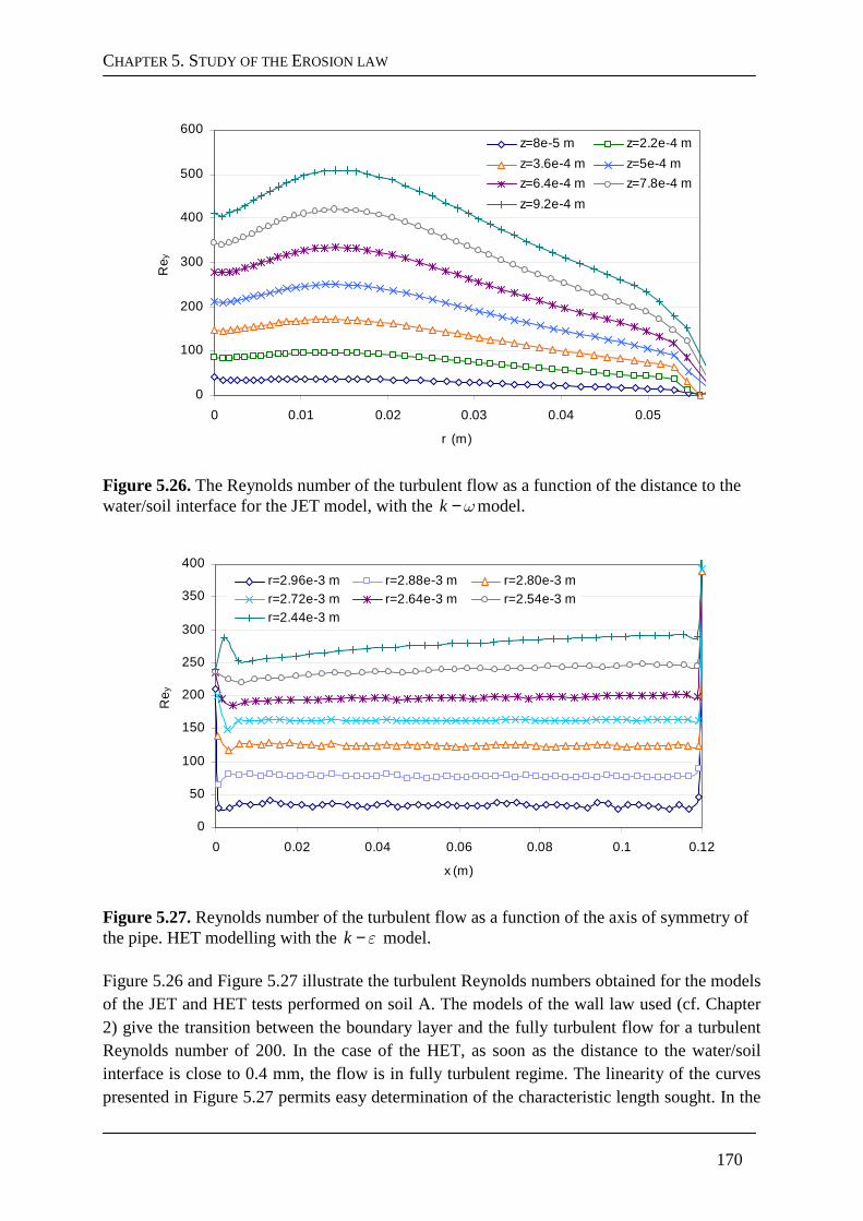
CHAPTER 5. STUDY OF THE EROSION LAW
170
0
100
200
300
400
500
600
0 0.01 0.02 0.03 0.04 0.05
r (m)
Re y
z=8e-5 m z=2.2e-4 m
z=3.6e-4 m z=5e-4 m
z=6.4e-4 m z=7.8e-4 m
z=9.2e-4 m
Figure 5.26. The Reynolds number of the turbulent flow as a function of the distance to the water/soil interface for the JET model, with the k ω− model.
0
50
100
150
200
250
300
350
400
0 0.02 0.04 0.06 0.08 0.1 0.12
x (m)
Re
y
r=2.96e-3 m r=2.88e-3 m r=2.80e-3 mr=2.72e-3 m r=2.64e-3 m r=2.54e-3 mr=2.44e-3 m
Figure 5.27. Reynolds number of the turbulent flow as a function of the axis of symmetry of the pipe. HET modelling with the k ε− model. Figure 5.26 and Figure 5.27 illustrate the turbulent Reynolds numbers obtained for the models of the JET and HET tests performed on soil A. The models of the wall law used (cf. Chapter 2) give the transition between the boundary layer and the fully turbulent flow for a turbulent Reynolds number of 200. In the case of the HET, as soon as the distance to the water/soil interface is close to 0.4 mm, the flow is in fully turbulent regime. The linearity of the curves presented in Figure 5.27 permits easy determination of the characteristic length sought. In the
CHAPTER 5. STUDY OF THE EROSION LAW
171
case of the JET, the characteristic length making it possible to situate the transition between the boundary layer and the fully turbulent flow depends on the distance to the jet centreline. For a distance to the water/soil interface close to 0.5 mm, more than 50% of the mesh cells are located above the transition Re 200y > . Thus, it is necessary to develop a complex analytical or numerical model to obtain an estimation of the pressure fluctuations, a variable identified as being susceptible to influence erosion. This could be one of the future perspectives of this work. In view of the results, it appears that taking into account the pressure gradient or a parameter linked to turbulence in the erosion law could allow us to develop a law for two tests of equivalent erosion parameters. However, major scientific and technical problems must be overcome before taking into account such variables in the erosion law.
5.3.2. Taking fluctuations into account in the stag nation region
The hypothesis of the non uniformity of the water/soil interface in the reality of the JET is one element in explaining the smoothing of the soil peak at the level of the stagnation point. However, improving the erosion law would enable solving this problem set out in paragraph 2.3.2. It is also necessary to take into account the fluctuations of the position of the stagnation point due to the turbulence in the erosion law. This should affect all the shear stress values in the erosion law and certainly all the other flow variables with which, potentially, it could be completed. Taking into account shear stress fluctuations, or any other parameter that could be considered in the erosion law, can be done by the convolution of the flow variable by a Gaussian curve, given the random displacement of the stagnation point around the jet centreline. The standard deviation and the variance could, for example, be calculated as a function of the fluctuations of the shear stress, the pressure or the intensity of the turbulence calculated above the water/soil interface, around the stagnation point. These corrective parameters should depend on the angle of shear stress, so that the model can be adapted to the presence and absence of the stagnation region of the flow. To our knowledge, the literature does not include studies allowing the estimation of these fluctuations in a configuration such as that of the JET. Taking these fluctuations into account is necessary but certainly not enough to obtain a unified erosion law. The numerical modelling of the JET shows that the order of magnitude of the erosion parameters is independent from them since it is related to the maximum shear stress at the outlet of the jet stagnation region. A major study aimed at characterising and estimating these fluctuations could be among the future perspectives of this thesis.
CHAPTER 5. STUDY OF THE EROSION LAW
172
5.3.3. Taking into account the pressure gradient in the erosion law
The addition of a component related to the tangential component of the pressure gradient in the erosion law seems to be a good path towards building one capable of unifying its different elements. As the data required can be obtained using the modelling method developed in Chapter 2, the objective of this final paragraph is to push this theory to the limit of the possibilities provided by our numerical models. The open question of the characteristic length related to the pressure gradient in the case of the JET is decisive. The generalised erosion law defined in equation (5.1) also points to the problem of the position of the eroded region along the water/soil interface in the case of the JET. Figure 5.28 illustrates the results obtained for the erosion rate as a function of the tangential component of the pressure gradient, as in the graph presented in Figure 5.9 which shows the erosion rate as a function of shear stress. The erosion rates obtained during the modelling of the JET and HETs performed on soil A are represented as a function of the gradients obtained numerically. The erosion rates obtained numerically are in good agreement with the experimental results (cf. Chapters 3 and 4). That is why we can estimate the orders of magnitude of the erosion parameters that allow maintaining the evolutions of the water/soil interface similar to those obtained for Eq. (1.1). The angular coefficients of the curves of Figure 5.28 give the order of magnitude of the erosion coefficients that would be obtained with an erosion law as a function only of the tangential component of the pressure gradient. The results obtained for different positions on the water/soil interface are studied at r fixed close to the jet stagnation point at 0.002 m, at the outlet of the stagnation region at 0.01 m and far from the stagnation region at 0.02 m. Two characteristic discretisation lengths of the gradient were tested for the JET, on the scale of the cell (spacing of 0.16 mm) and on the scale of 20 cells (spacing of 3 mm). Figure 5.28 confirms the fact that the orders of magnitude of the results obtained are very close for the two scales tested and for three positions on the interface. The angle coefficients of the curves corresponding to the results of the JET and the HET are of the order of 10-9 and 10-10 m3.s/kg, respectively. The erosion thresholds obtained remain in the same order of magnitude for the JET and the HET, as in the case of Eq. (1.1). They are both close to 5.104 Pa/m. These erosion coefficient and erosion threshold values are not comparable to those obtained in the framework of Eq. (1.1). Thus this study of orders of magnitude shows that the development of an erosion law defined by equation (5.1) with ( )rψ as the tangential component of the pressure gradient does not permit obtaining unified erosion parameters for the JET and HETs performed on soil A. The erosion coefficient obtained for the JET was again at least one order of magnitude higher than that found for the HET, cf. Figure 5.28. Furthermore, if we define ( )rψ as a function dependent on the tangential component of the pressure gradient and the shear stress, the variance obtained for the erosion parameters of the JET and the HET would also be higher.
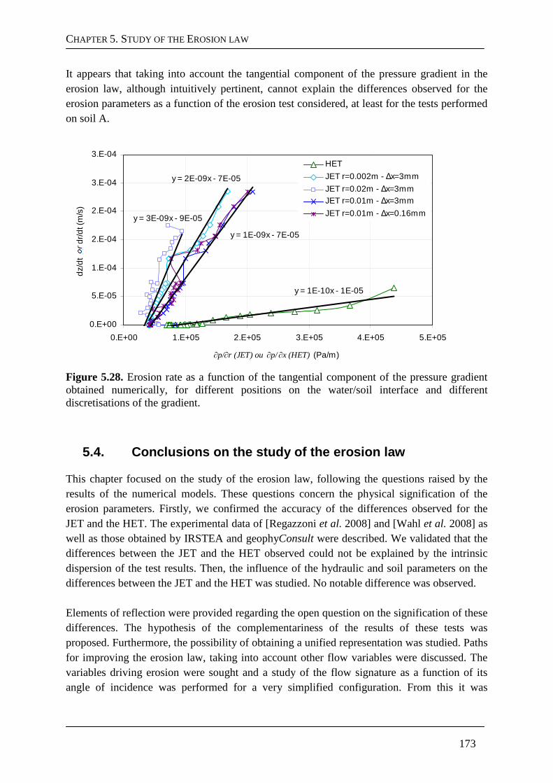
CHAPTER 5. STUDY OF THE EROSION LAW
173
It appears that taking into account the tangential component of the pressure gradient in the erosion law, although intuitively pertinent, cannot explain the differences observed for the erosion parameters as a function of the erosion test considered, at least for the tests performed on soil A.
y = 1E-10x - 1E-05
y = 2E-09x - 7E-05
y = 1E-09x - 7E-05
y = 3E-09x - 9E-05
0.E+00
5.E-05
1.E-04
2.E-04
2.E-04
3.E-04
3.E-04
0.E+00 1.E+05 2.E+05 3.E+05 4.E+05 5.E+05
∂p/∂r (JET) ou ∂p/∂x (HET) (Pa/m)
dz/
dt o
u d
r/d
t (m
/s)
HET
JET r=0.002m - ∆x=3mm
JET r=0.02m - ∆x=3mmJET r=0.01m - ∆x=3mm
JET r=0.01m - ∆x=0.16mm
Figure 5.28. Erosion rate as a function of the tangential component of the pressure gradient obtained numerically, for different positions on the water/soil interface and different discretisations of the gradient.
5.4. Conclusions on the study of the erosion law
This chapter focused on the study of the erosion law, following the questions raised by the results of the numerical models. These questions concern the physical signification of the erosion parameters. Firstly, we confirmed the accuracy of the differences observed for the JET and the HET. The experimental data of [Regazzoni et al. 2008] and [Wahl et al. 2008] as well as those obtained by IRSTEA and geophyConsult were described. We validated that the differences between the JET and the HET observed could not be explained by the intrinsic dispersion of the test results. Then, the influence of the hydraulic and soil parameters on the differences between the JET and the HET was studied. No notable difference was observed. Elements of reflection were provided regarding the open question on the signification of these differences. The hypothesis of the complementariness of the results of these tests was proposed. Furthermore, the possibility of obtaining a unified representation was studied. Paths for improving the erosion law, taking into account other flow variables were discussed. The variables driving erosion were sought and a study of the flow signature as a function of its angle of incidence was performed for a very simplified configuration. From this it was
CHAPTER 5. STUDY OF THE EROSION LAW
174
deduced that the variables driving erosion may be shear stress the pressure gradient or pressure fluctuations. Then, paths for developing the erosion law were explored. It was verified that the flow mechanical quantities determined previously also present significant differences for the JET and HET configurations (except for the pressure fluctuations for which we had no estimation). Two paths for developing the erosion law were then studied. The first concerned taking into account the fluctuations due to the turbulence in the jet stagnation region and the bases of such an improvement were set out. Taking the pressure gradient into account in the erosion law was also proposed though no element was found to validate this theory.
175
CONCLUSION
This thesis was dedicated to the numerical modelling of erosion phenomena in the context of studying the safety of embankment dams and dikes. The objective of this work was to develop a numerical method to model the erosion of a cohesive soil by a turbulent flow. The method developed was then applied to modelling the Jet Erosion Test, in order to conclude on the pertinence of its interpretation model. A comprehensive state of the art on the general context of breaches in hydraulic structures, interpretation models and the devices used for the Jet and Hole Erosion Tests was provided. In addition, the subject of modelling mobile interfaces was dealt with. The interpretation model developed by [Bonelli et al. 2006] for the Hole Erosion Test and the model developed by [Hanson and Cook 2004] for the Jet Erosion Test were described. After this the different erosion laws in the literature were reviewed. Many of the empirical laws could not be adapted efficiently for our flow configurations. Models based on the fundamental equations of biphasic flows were considered as the basis for developing a new erosion model. In addition, the choice of the modelling method relied on elements in the literature covering the modelling of mobile interfaces. Preference was given to choosing a mobile interface model with adaptive meshing rather than one with a fixed mesh. The numerical modelling method developed was then explained with a description given of the main equations of the Navier-Stokes equations for turbulent flows with an adapted mesh. RANS models, turbulence models and the treatment of the wall implemented in the ANSYS Fluent CFD software were then described. The sequential modelling method uncoupled from erosion was described and justified, as was the implementation of the interface displacement laws. The limits of the so-called classical erosion law were described. This erosion law was considerably modified to offset the inconsistencies it presented in the case of normal flows. The non uniformity of the real phenomena and the fluctuations of the position of the jet stagnation point due to turbulence permitted justifying this modification. This was followed by an explanation of the discretisation and remeshing methods used. The major difficulties encountered during the development of this erosion model were described. The results obtained on normal flows were presented and the independence from the meshing and the influence of the model were studied. As from a given mesh density, at different levels of the calculation domain, the results given by the model without erosion were independent from the mesh to within 5%. Regarding the choice of turbulence model, the results obtained were compared with the results from the literature for the flow velocity at the jet centreline, the shear stress and the pressure at the water/soil interface. Globally, the RSM model presented the best fit with the experimental results, however the difficulties encountered when implementing it and its long calculation times prevented us from using it for modelling with erosion. The k-ε and k-ω turbulence models appeared complementary, and in comparison with the other two turbulence
CONCLUSION
176
models tested, the first gave the results closest to those in the literature on shear stress, while the second was closest to the results in the literature on pressure and flow velocity. Finally, we opted to use these two models in parallel to model the JET tests. Three JET tests were performed on three different soils. Whatever the test carried out, the numerical results obtained with the k-ω turbulence model were in good agreement with the experimental results and those given by the semi-empirical model of [Hanson and Cook 2004]. Relative errors lower than 25% were observed for the scour depths. The results given by the k-ε model were less close to the experimental and semi-empirical results but nonetheless presented the same order of magnitude. This study also permitted describing the recirculation phenomena present when the curvature of the water/soil interface became pronounced. A parametric study was performed to estimate the errors on the numerical results in the case of variations of the erosion parameters. It was shown that the range of erosion parameters for which the numerical results remained in good agreement was very limited and strongly dependent on the values of the erosion parameters. The lower the erosion parameters, the more a variance of only a few percent on these parameters was susceptible to lead to errors of more than 100% on the scour depth and the erosion kinetics. This result was important since it permitted validating the pertinence of the modelling method. It also showed that the erosion parameters obtained following the JET tests, apart from a relative error of a few percent, permit obtaining the evolution of the erosion figure obtained experimentally. The erosion coefficient and the critical shear stress obtained with the interpretation model of [Hanson and Cook 2004], following complex numerical modelling, were used to find the evolution of the erosion figure obtained experimentally. This result is an important element for validating the interpretation model of the JET. However, the numerical model could not be used to deduce the physical signification of these parameters. The results obtained for the tangential flows were presented. First, the method was validated in the case of a laminar flow for a theoretical case: the erosion of a channel in laminar regime. The numerical results obtained agreed with the theoretical results to within 2%, and likewise in the case of a pipe 1 m long and in that of a pipe 1 cm long. These results represented a major validation of the modelling method we developed. In the framework of HET modelling, the independence of the results from the mesh density were studied, as was the influence of the turbulence model. Contrary to the jet flow, which is more complex, the results of the three turbulence models gave similar results. The models of the flow with erosion were performed only with the k-ε turbulence model. Then, the HET tests were modelled. The first model concerned the HET test performed on soil A, for which the JET test was also modelled. The two other tests were performed on two other soils. Good agreement between the numerical results and the numerical and experimental results given by the analytical model of [Bonelli et al. 2006] was obtained. The numerical results obtained for the pressure differential between sections A and B differed from the experimental results by a relative error of less than 10% in comparison to the initial pressure differential.
CONCLUSION
177
A parametric study was also performed to evaluate the range of parameters for which the numerical results were in good agreement with the experimental ones. As with the results obtained for the JET, it was deduced from this study that the lower the erosion parameters were, the higher the error generated on the evolution of the pressure would be. Thus only the erosion parameters implemented led to numerical results in good agreement with the experimental results, within a margin of error of only a few percent. This result was an important element for validating the modelling method developed and the interpretation model of [Bonelli et al. 2006]. In view of the results of the numerical models of the JET and HET tests, it was concluded that the erosion parameters found for each test permitted finding the evolution of the erosion scour holes during each of these tests. Nonetheless, for the same soil, such as soil A modelled for the two tests, the erosion parameters differed by one order of magnitude. This meant that: i) these parameters were related to the test and depended on the angle of incidence of the hydraulic stress; and that ii) a complementary study was necessary to determine the physical signification of the erosion parameters found. An analysis of the erosion law and erosion parameters obtained following the JET and HET tests was begun. The differences obtained for the erosion parameters for the different soils and by different laboratories were analysed. No obvious influence of the flow parameters or the soil characteristics on the differences between the JET and the HET could be identified. However, we observed that in the case of ¾ of the tests recorded, the same type of soil was found to be more erodible with the JET that with the HET. The erosion coefficient found was generally higher with the JET by one or two orders of magnitude than that found with the HET. Conversely, the critical shear stress was often lower by one or two orders of magnitude. A test campaign was carried out on mixtures of kaolinite and Hostun sand and consisted in a repeatability study of JET tests. The results were sometimes dispersed over one order of magnitude for the critical shear stress found following the JETs. However, the results obtained with the HET remained very different from those obtained with the JET, error margins included. We deduced that the differences between the JET and the HET were significant and could not be imputed to error margins intrinsic to the tests. Afterwards, an analysis of the variables susceptible to influence erosion was performed. By assuming that the anisotropy of the material was not responsible for these differences, the flow variables on which erosion may depend were identified. An in-depth numerical study of the flow signature without erosion in a very simplified configuration was performed and the results obtained for different flow mechanical quantities as a function of the impinging angle of the flow were presented. It was deduced that the flow variables most susceptible to drive erosion were shear stress, the tangential component of the pressure gradient and the pressure fluctuations due to the turbulence above the boundary layer. We did not have any estimation for the latter. Paths for developing the erosion law were then explored. The flow variables obtained for the JET and HET numerical models on soil A were compared. The problem of improving the erosion law with respect to the stagnation region of the JET, in the case of a unified erosion law whatever the angle of stress exerted by the flow on the soil was discussed. The option of
CONCLUSION
178
improving the erosion law by taking into account the tangential component of the pressure gradient was suggested. The results obtained did not lead to concluding in favour of this possibility of improving the erosion law. Nonetheless, the bases of a study on the influence of the angle of incidence of the flow on the efficiency of erosion were set out.
179
OUTLOOK FOR FURTHER RESEARCH
The outlook for the work done in this thesis could involve, firstly, improving the physical model used in our modelling, by: i) Taking into account the roughness of the water/soil interface. We first considered an approximation of the water/soil interface as a smooth wall. However, the approach developed by [Cebeci and Bradshaw 1997] applied to our flow configurations demonstrated that roughness starts having an influence on the interface if the height of the asperities exceeds 10 µm . It would be interesting to develop a numerical (and experimental) approach to study the influence of roughness on erosion phenomena. ii) Implementing the RSM model. Major problems of divergence in the calculations and enormous increases in calculation time do not at present permit modelling the entire erosion process with an RSM model. The results obtained for this turbulence model are nonetheless reputed to be more reliable than those obtained with two equation models. Additional research could perhaps lead to this more advanced turbulence model for modelling the erosion process. Improving the numerical model and optimising the calculation times could also be included in the outlook for the work of this thesis, by: i) Refining the convergence criteria. Whatever the micro-remeshing considered, the convergence criterion of the fluid calculation is fixed throughout the calculation. Moreover, it was determined more or less arbitrarily. Automating the calculation of the fluid/deformation process in the software effectively makes defining the number of iterations required as a function of the convergence of the residues a complex task. This point could be reworked to optimise the calculation time. ii) Optimising the limiters. Numerical criteria were imposed in the interface displacement code to favour the convergence of the calculation. The first limiter was related to the CFL type condition. The displacement of a node cannot exceed a tenth of the size of the adjacent cell. The second is related to the erosion time step, whose increment cannot exceed 1.001 times the previous time step. The calculation time could be optimised by adjusting these limiters, with the criteria being established on the basis of convergence, for example. In addition, the following proposals could deepen certain issues raised during the work performed in the framework of this thesis: i) Additional numerical and/or experimental research on changes of regime inside a cavity could be performed. The regimes obtained will be studied as a function of the geometric parameters of the cavity and the flow parameters. This would certainly lead to the development of a new law making it possible to predict the flow regime (Strongly Deflected or Weakly Deflected) during the erosion process. ii) The range of erosion parameters for which the interpretation models are verified could also be widened. The tests modelled are quite representative of the materials that are really tested in the JET and HET. However, it could be asked whether the conclusion reached regarding
OUTLOOK FOR FURTHER RESEARCH
180
the pertinence of the interpretation models are still valid for extremely erodible soils or, on the contrary, for extremely resistant ones. iii) In view to improving the repeatability of the JETs, attempts should be made to perform these tests with a larger quantity of soil and a larger test mould. It appeared that the more the final scour depths are close to and greater than the dimensions of the mould, the higher the repeatability errors of the test are. This point must be verified experimentally. iv) The study of the singularities of the differences between the JET and the HET for the tests carried out by IRSTEA/geophyConsult could be deepened. We observed that a large number of erosion tests carried out in our laboratories resulted in more erosion for the HET than for the JET. A wider range of results would permit concluding on the representativeness of this singularity of the results obtained by IRSTEA/geophyConsult. However the main perspectives visible following the works of this thesis above all concern the development of the study on the erosion law, with: i) The determination of the influence of the flow variables and soil parameters on the differences between the JET and the HET. To study the influence of water content, density and boundary conditions in depth, a major test campaign is necessary in which the influence of each variable would be studied, all things being equal elsewhere. ii) The fine modelling of the fluctuation of the position of the stagnation point and the non uniformity of the soil. An experimental study would lead to better understanding of the phenomena involved. If the erosion of a soil is really driven by the shear stress exerted by the water on the soil, it would be interesting to demonstrate the smoothing of the theoretical non eroded soil peak. Even in the case of other variables driving erosion, better understanding erosion mechanisms under a jet flow would be a major step forward. iii) The development of research in view to formulating a unifying erosion law for all types of flow, with as essential elements the determination of erosion modes and the erosion of the variables driving erosion. A very thorough experimental study of the erosion of cohesive soils would certainly provide elements of response to these questions. In particular, it could result in the formulation of a model for pressure and shear stress fluctuations.
181
REFERENCES
Aderibigde O. and Rajaratnam N., Erosion of loose beds by submerged circular impinging vertical turbulent jets, Journal of Hydraulic Research, IAHR, 34(1):19-33, 1996.
Allen P. M., Arnold J. and Jakubowski E., Design and testing of a simple submerged jet device for field determination of soil erodibility, Environmental and Engineering Geoscience, 3(4):579−584, 1997.
Angot P., A unified ficititious domain model for general embedded boundary conditions, Compte-rendus de l’Académie des sciences de Paris, I341:683-688, 2005.
Annandale G., How does water-soil interaction lead to erosion ?, In Geo-Denver 2007: New Peaks in Geotechnics, 2007.
Ansys, Fluent Theory Guide Release 12.0, ANSYS Inc., 2009.
Antonia R. A., Kim J. and Browne L. W. B., Some characteristics of small-scale turbulence in a turbulent duct flow, J. Fluid Mech, 233:369-388, 1991.
Ariathurai R. and Arulanandan K., Erosion rates of cohesive soils, Journal of the Hydraulics Division, 104(2):279-283, 1978.
Balabel A. and El-Askary W. A., On the performance of linear and nonlinear k–ε turbulence models in various jet flow applications, European Journal of Mechanics B/Fluids, 30:325–340, 2011.
Bagnold R. A., The flow of cohesionless grains in fluids, Phil. Trans. of Royal Society of London, 249(964):235-297, 1956.
Barekyan A. S., Discharge of channel forming sediments and elements of sand waves, Soviet Hydrol, Selected Papers (Transactions of AGU n°2), 128-130, 1962.
Barth T. J. and Jespersen D., The design and application of upwind schemes on unstructured meshes, Technical Report AIAA-89-0366, AIAA 27th Aerospace Sciences Meeting, Reno, Nevada, 1989.
Beek V., Bezuijen A. and Sellmeijer H., Backward erosion piping, Erosion in Geomechanics Applied to Dams and Levees, Wiley/ISTE, 193-271, 2013.
Bell B., Turbulent Flow Case Studies, Fluent Inc., Fluent Software Training, 2003.
Beltaos S. and Rajaratnam N., Impinging circular turbulent jets, J. Hydraulic Div., ASCE, 100(HY10):1313–1328, 1974.
Beguin R., Philippe P., Faure Y. H. and Guidoux C., Contact erosion between two soils, in Erosion of Geomaterials, Wiley/ISTE, 115-154, 2012.
Benahmed N., Chevalier C. and Bonelli S., Chapitre 5 - Erosion par écoulement localisé dans un conduit, in Erosion des géomatériaux, Traité MIM série Risques Naturels, Hermès Science Publication, 37 p., 2012.
Benahmed N. and Bonelli S., Investigating concentrated leak erosion behaviour of cohesive soils by performing hole erosion tests, European Journal of Environmental and Civil Engineering, 16(1):43-58, 2012.
Blaisdell F. W., Clayton L. A. and Hebaus G. G., Ultimate dimension of local scour, J. Hydraulics Division, ASCE, 107(HY3):327−337, 1981.
REFERENCES
182
Bollaert E., Transient water pressure in joints and formation of rock scour due to High-Velocity Jet Impact, Communication n°13, Laboratory of Hydraulic Constructions, Ecole Polytechnique Federale de Lausanne, 2002.
Bonelli S. and Brivois O., The scaling law in the hole erosion test with a constant pressure drop, International Journal for Numerical and Analytical Methods in Geomechanics, 32:1573-1595, 2008.
Bonelli S., Brivois O., Borghi R. and Benahmed N., On the modelling of piping erosion, Comptes Rendus de Mécanique, 8-9(334):555-559, 2006.
Bonelli S., Golay F. and Mercier F., Chapter 6 - On the modelling of interface erosion, in Erosion of Geomaterials, Wiley/ISTE, 187-222, 2012.
Briaud J.-L., Ting F. C. K., Chen H. C., Cao Y., Han S. W. and Kwak K. W., Erosion function apparatus for scour rate predictions, Journal of Geotechnical and Geoenvironmental Engineering, 127(2):105-113, 2001.
Briaud J.-L., Chen H. C., Govindasamy A. V. and Storesund R., Levee erosion by overtopping in New Orleans during the Katrina Hurricane, Journal of Geotechnical and Geoenvironmental Engineering, 134(5):618-632, 2008.
Brivois O., Contribution à la modélisation de l'érosion de fortes pentes par un écoulement turbulent diphasique. Thèse de doctorat, Université de la Méditerranée, 2005.
Buffington J. M. and Montgomery D. R., A systematic analysis of eight decades of incipient motion studies, with special reference to gravel-bedded rivers, Water Resources Research, 33(8):1993–2029, 1997.
Cao Z., Explicit formulation of the Shields diagram for incipient motion of sediment, Journal of Hydraulic Engineering, 132(10), 2006.
Cebeci T. and Bradshaw P., Momentum transfers in boundary layers hemisphere, Pub. Corp., 391p, 1977.
Chang D. S. and Zhang L. M., Simulation of the erosion process of landslide dams due to overtopping considering variations in soil erodibility along depth, Nat. Hazards Earth Syst. Sci., 10:933–946, 2010.
Chauchat J. and Médale M., A three-dimensional numerical model for incompressible two-phase flow of a granular bed submitted to a laminar shearing flow, Comput. Method. Appl. M., 199(9-12):439-449, 2010.
Chen H. C. and Patel V. C., Near-Wall Turbulence Models for Complex Flows Including Separation, AIAA Journal, 26(6):641–648, 1988.
Chorin A. J., Numerical solution of Navier-Stokes equations, Mathematics of Computation, 22:745-765 1968.
Claudin P. and Andreotti B., A scaling law for aeolian dunes on Mars, Venus, Earth; and for subaqueous ripples, Earth and Planetary Science Letters, 252:30-44, 2006.
Cleaver J. W. and Yates B., Mechanism of detachment of colloid particles from a flat substrate in turbulent flow, J. Colloid Interface Sci., 44:464-474, 1973.
Craft T., Graham L. and Launder B., Impinging jet studies for turbulence model assessment – II. An examination of the performance of four turbulence models, Int. J. Heat Mass Transfer, 36(10), 1993.
REFERENCES
183
Croad R. N., Physics of erosion of cohesive soils, Phd Thesis, Departement of Civil Engineering, University of Auckland, Auckland, New Zeland., 1981.
Dade W., Nowell A. and Jumars P., Predicting erosion resistance of muds, Marine Geology, 105:285-297, 1992.
DeBar R., A method in two-d eulerian hydrodynamics, Technical Report LA-3425, Los Alamos Scientific Laboratory, University of California, 1974.
Dey S. and Westrich B., Hydraulics of submerged jet subject to change in cohesive bed geometry, Journal of Hydraulic Engineering, 129(1), 2003.
Donea J., Guiliani S. and Halleux J. P., An arbitrary lagrangian eulerian finite element method for transcient dynamics fluid structure interaction, Comp. Meth. Appl. Mech. Eng., 33:689-723, 1982.
Du Boys P., Le Rhône et les Rivières à Lit Affouillable, Annales des Ponts et Chaussées, Série 5, 18:141-195, 1879.
Dunn I. S., Tractive resistance of cohesive channels, J. Soil Mech. and Foundations Div., Proc. Am. Soc. Civil Engrs, 1-24, 1959.
Einstein H. A., The Bed-Load function for sediment transportation in open channel flows, Technical Bulletin No. 1026, U.S. Departement of Agriculture, Soil Conservation Service, Washington D.C., 1950.
Engelund F. and Hansen E., A monograph on sediment transport in alluvial streams, Teknisk Forlag, Copenhagen, Denmark, 65p, 1967.
Emmerling R., The instantaneous of the wall pressure under a turbulent boundary layer flow, Max-Planck-Institut fur Stromungsforschung, Rep. No. 9, 1973.
Fell R. and Fry J.-J., International erosion and dams and their foundations, Taylor & Francis, Oxon, Royaume-Uni, 2007.
Fell R., Hanson G., Herrier G., Marot D. and Wahl T., Relationship between the erosion properties of soils and other parameters, In Erosion in Geomechanics Applied to Dams and Levees, Wiley/ISTE, 343-382, 2013.
Foster M., Fell R. and M. S., The statistics of embankment dam failures and accidents, Canadian Geotechical Journal, 37:1000-1024, 2000.
Fry J.-J., Chapitre 1 - Introduction à l'érosion interne dans les barrages et les digues, Erosion des géomatériaux, Traité MIM série Risques Naturels, Hermès Science Publication, 36 p., 2012.
Gargani J., Contribution à l'étude de la vitesse critique d'érosion des sols cohésifs, C. R. Geosciences, 336:561-566, 2004.
Geers L. F. G., Hanjalic K. and Tummers M. J., Wall imprint of turbulent structures and heat transfer in multiple impinging jet arrays, J. Fluid Mech., 546:255–284, 2006.
Gibbs H. J., A study of erosion and tractive force characteristics in relation to soil mechanics properties, Soils Engineering Rep. No. EM-643, United States Dept. of the Interior, Bureau of Reclamation, Division of Engineering Laboratories, Denver, 1962.
Görtler H., Über eine dreidimensionale Instabilität laminarer Grenzschichten an konkaven Wändern, Nachr. Wiss. Ges. Göttingen, Math. Phys. Klasse, Neue Folge 2, No. 1, 1941.
REFERENCES
184
Hadziabdic M. and Hanjalic K., Vortical structures and heat transfer in a round impinging jet, J. Fluid Mech., 596:221–260, 2008.
Haehnel R. and Dade W., Physics of particle entrainment under the influence of an impinging jet, U.S. Army Engineer Research and Development Center Cold Regions Research and Engineering Laboratory Hanover, NH 03755, 2008.
Hanson G. J., Development of a jet index to characterize erosion resistance of soils in earthen spillways, Transactions of the ASAE, 34(5):2015−2020, 1991.
Hanson G. J. and Cook K. R., Apparatus, Test Procedures and Analytical Methods to Measure Soil Erodibility In Situ, Engineering in Agriculture, ASAE, 20(4):455-462, 2004.
Hanson G. J. and Robinson K. M., The influence of soil moisture and compaction on spillway erosion, Transactions of the ASAE, 36(5):1349−1352, 1993.
Hanson G. J., Robinson K. M. and Temple D. M., Pressure and Stress Distributions Due to a Submerged Impinging Jet, Res. Hydr. Engr. USDA, 1990.
Hanson G. J. and Simon A., Erodibility of cohesive streambeds in the loess area of the Midwestern USA, Hydrological processes, 15(1):23-38, 2001.
Hénensal P., Recherches qui pourraient être entreprises en génie civil dans le domaine de l’érosion et de l’érodabilité hydrique des sols, Rapport interne LCPC, FAER 1.04.03.3, 21 p., 1983.
Hinze J. D., Turbulence, 2nd Edition Mcgraw-Hill, New York, 1975.
Hoffmans G., The influence of turbulence on soil erosion, Eburon Academic Publishers, 2012.
Hogg A. J., Huppert H. E. and Dade W. B., Erosion by planar turbulent wall jets, Jounal of Fluid Mechanics, 338:317-340, 1997.
Hollick M., Towards a routine test for the assessment of critical tractive forces of cohesive soils, Transactions of the ASAE, 19(6):1076−1081, 1976.
Holmes D. G. and Connell S. D., Solution of the 2D Navier-Stokes Equations on Unstructured Adaptive Grids, Presented at the AIAA 9th Computational Fluid Dynamics Conference, 1989.
Hopfinger E. J., Kurniawan A., Graf W. H. and Lemmin U., Sediment erosion by Görtler vortices: the scour-hole problem, Journal of Fluid Mechanics, 520:327-342, 2004.
Indraratna B., Muttuvel T. and Khabbaz H., Modelling the erosion rate of chemically stabilized soil incorporating tensile force - deformation characteristics, Canadian Geotechical Journal, 46:57-68, 2009.
Jackson R., The dynamics of fluidized particles, Cambridge University Press, 2000.
Jaramillo J. E., Pérez-Segarra C. D., Rodriguez I. and Olivia A., Numerical Study of Plane and Round Impinging Jets Using RANS Models, Numerical Heat Transfer, 213-237, 2008.
Kader B., Temperature and Concentration Profiles in Fully Turbulent Boundary Layers, Int. J. Heat Mass Transfer, 24(9):1541–1544, 1981.
Kim J., Moin P. and Moser R., Turbulence statistics in fully developed channel flow at low Reynolds number, J. Fluid Mech, 177:133-166, 1987.
REFERENCES
185
Kobus H., Liester P. and Westrich B., Flow field and scouring effects of steady and pulsating jets impinging on movable bed, Journal of Hydraulic Research, IAHR, 17(3):175-192, 1979.
Lachouette D., Golay F. and Bonelli S., One-dimensional modelling of piping flow erosion, Comptes Rendus de Mécanique, 336:731-736, 2008.
Langendoen E. J., Simon A. and Alonso C. V., Modelling channel instabilities and mitigation strategies in Eastern Nebraska, Proc. of the 2000 Joint Conference on Water Resources Engineering and Water Resource Planning and Management, (CD−ROM). New York: ASCE, 2000.
Launder B. E. and Spalding D. B., Lectures in Mathematical Models of turbulence Academic Press London, 1972.
Lefebvre G., Rohan K. and Douville S., Erosivity of natural intact structured clay: evaluation, Canadian Geotechical Journal 22:508-517, 1985.
Looney M. K. and Walsh J. J., Mean-flow and Turbulent Characteristics of Free and Impinging Jet Flow, J. Fluid Mech, 147:397-429, 1984.
Marot D. and Benamar A., Suffusion, transport and filtration of fine particles in granular soil, In Erosion of Geomaterials, Wiley/ISTE, 39-80, 2012.
Mazurek K. A., Rajaratnam N. and Sego D. C., Scour of cohesive soil by submerged circular turbulent impinging jets, J. Hydraulic Engineering, 127(7):598−606, 2001.
Mazurek K. A. and Hossain T., Scour by jets in cohesionless and cohesive soils, Canadian Journal of Civil Engineering, Special Issue on Hydrotechnical Engineering, 34:744-751, 2007.
Mercier F., Bonelli S., Anselmet F., Pinettes P., Courivaud J.-R. and Fry J.-J., On the numerical modelling of the Jet Erosion Test, ICSE6, Paris, 2012.
Mercier F., Golay F., Bonelli S., Anselmet F., Borghi R. and Philippe P., Numerical modelling of the erosion of a cohesive soil by a turbulent impinging jet, soumis-a.
Mercier F., Bonelli S., Pinettes P., Golay F., Anselmet F. and Philippe P., Comparison of CFD simulations with experimental Jet Erosion Tests results, soumis-b.
Mercier F., Bonelli S., Golay F., Anselmet F., Philippe P. and Borghi R., Numerical modelling of concentrated leak erosion during Hole Erosion Tests, soumis-c.
Meyer-Peter E. and Müller R., Formulas for bed-load transport, Proceedings of the Second Meeting of IAHR, 39-64, 1948.
Moore W. L. and Masch F. D., Experiments on the scour resistance of cohesive sediments, J. Geophysical Research, 67(4):1437−1446, 1962.
Narumanchi S. V. J., Hassani V. and Bharathan D., Modelling Single-Phase and Boiling Liquid Jet Impingement Cooling in Power Electronics, Technical Report NREL, TP-540-38787, 2005.
Nearing M. A., A probabilistic model of soil detachment by shallow turbulent flow, Trans. ASCE, 34:81-85, 1991.
O'Donoghue T., Trajkovic B. and Piggins J., Sand bed response to submerged water jet, Proc. 11th International Offshore and Polar Engineering Conference, Norway, 2001.
Osher S. and Sethian J., Fronts propagating with curvature dependent speed: algorithm for tracking material interface, Journal of Computational Physics, 39:201-225, 1981.
REFERENCES
186
Ouriemi M., Aussillous P. and Guazzelli E., Sediment dynamics. Part1. Bedload transport by laminar shearing flows, Journal of Fluid Mechanics, 636:295-319, 2009.
Paaswell R. E., Causes and mechanisms of cohesive soil erosion: state of art, Special report 135, Highway Research Board, National Research Council, D.C., 52-74, 1973.
Papamichos E. and Vardoulakis I., Sand erosion with a porosity diffusion law, Computers and Geotechnics, 32:47–58, 2005.
Partheniades E., Erosion and Deposition of Cohesive Soils, Journal of Hydraulic Division, 91:105-139, 1965.
Patankar S. V. and Spalding D. B., A calculation procedure for heat, mass ant momentum transfers in three-dimensional parabolic flows, Int. J. Heat Mass Transfer, 15, 1972.
Peskin C. S., The immersed boundary method, Acta numerica, 1-39, 1977.
Phares D. J., Smedley G. T. and Flagan R. C., The wall shear stress produced by the normal impingement of a jet on a flat surface, J. Fluid Mech., 418:351-375, 2000.
Philippe P., Beguin R. and Faure Y. H., Contact erosion, in Erosion in Geomechanics Applied to Dams and Levees, Wiley/ISTE, 101-192, 2013.
Pinettes P., Courivaud J.-R., Fry J.-J., Mercier F. and Bonelli S., First introduction of Greg Hanson’s « Jet Erosion Test » in Europe: return on experience after 2 years of testing, USSD annual meeting, 2011.
Pope S. B., Turbulent Flows, Cambridge University Press, 2000.
Poreh M., Tsuei Y. G. and Cermak J. E., Investigation of a turbulent radial wall jet, Trans. ASME: J. Appl. Mech., 34:457-463, 1967.
Rajaratnam N., Erosion by submerged circular jets, Journal of Hydraulic Division, 108(HY2):262-267, 1982.
Rauch R. D., Batira J. T. and Yang N. T. Y., Spatial Adaption Procedures on Unstructured Meshes for Accurate Unsteady Aerodynamic Flow Computations, Technical Report AIAA-91-1106, 1991.
Raudkivi A. J., Loose Boundary hydraulics, Balkeman/Rotterdam/Brookfield, 1998.
Regazzoni P.-L. and Marot D., Investigation of interface erosion rate by Jet Erosion Test and statistical analysis, European Journal of Environmental and Civil Engineering, 15(8):1167-1185, 2011.
Regazzoni P.-L., Marot D., Wahl T., Hanson G. J. and Courivaud J.-R., Soils erodibility: a comparison between the Jet Erosion Test and the Hole Erosion Test, Proc. Inaugural International Mechanics Institute (EM08), Conference (A.S.C.E.), Minneapolis, USA, 2008.
Rickenmann D. and Recking A., Evaluation of flow resistance in gravel-bed rivers through a large field dataset, Water Resources Research, 47:1-23, 2011.
Robinson K. M., Bennett S. J., Hanson G. J. and Kadavy K. C., The influence of weathering on headcut erosion, ASAE Paper No. 002066. St. Joseph, Mich.: ASAE, 2000.
Rouse H., An analysis of sediment transportation in the light of fluid turbulence, Soil Conservation Services Report No. SCS-TP-25, USDA, Washington D.C., 1939.
Schlichting H., Boundary Layer theory, Springer, 1960.
Schoklitsch A., Uber Schleppkraft Und Geschiebebewegung, KESSINGER PUB LLC, 1914.
REFERENCES
187
Sharif A. R. and Atkinson J. F., Model for surface erosion of cohesive soils, Journal of hydraulic Engineering, 138(7):581-590, 2012.
Shields A., Anwendung der aenlichkeitsmechanik und der turbulenzforschung auf die geschiebebewegung, Mitteilungen der Preussischen Versuchsanstalt fur Wasserbau und Schiffbau, Berlin, Germany, translated to English by CalTech, Pasadena, CA, 1936.
Shih T.-H., Liou W. W., Shabbir A., Yang Z. and Zhu J., A New k-epsilon Eddy-Viscosity Model for High Reynolds Number Turbulent Flows - Model Development and Validation, Computers Fluids, 24(3):227–238, 1995.
Simon A. and Thomas R. E., Processes and forms of an unstable system with resistant, cohesive streambeds, J. Earth Surface Processes and Landforms, 27(7):699−718, 2002.
Smerdon E. T. and Beasley R. P., Critical tractive forces in cohesive soils, Agric. Eng., 26-29, 1961.
Stein O. R. and Nett D. D., Impinging jet calibration of excess shear sediment detachment parameters, Transactions of the ASAE, 40(6):1573−1580, 1997.
Ternat F., Boyer P., Anselmet F. and Amielh M., Erosion threshold of saturated natural cohesive sediments: Modelling and experiments, Water Resources Research, 44, W11434, 2008.
Tritton D. J., Physical Fluid Dynamics - 2nd edition, Oxford Science Publications, 1988.
Vardoulakis I., Stavropoulou M. and Papanastasiou P., Hydromechanical aspects of sand production problem, Transport in Porous Media, 22:225-244, 1996.
Viegas D. X. and Borges A. R. J., An Erosion Technique for the Measurement of the Shear Stress Field on a Flat Plat, Journal of Physics E: Scientific Instruments, 19(8):625-63, 1986.
Wahl T. L., Regazzoni P.-L. and Erdogan Z., Determining Erosion Indices of Cohesive Soils with the Hole Erosion Test and Jet Erosion Test, Dam Safety Office Report DSO-08-05, U.S. Dept. of the Interior, Bureau of Reclamation, Denver, CO, 2008.
Wan C. F. and Fell R., Investigation of internal erosion and piping of soils in embankment dams by the slot erosion test and the hole erosion test, UNICIV Report, no. R-412, 3-18, 2002.
Wan C. F. and Fell R., Laboratory Tests on the Rate of Piping Erosion of Soils in Embankment Dams, Journal of Geotechnical Testing Journal, 27(3):295-303, 2004.
Winterwerp J. C. and Van Kesteren W. G. M., Introduction to the Physics of Cohesive Sediment in the Marine Environment, Developments in Sedimentology Series no. 56. xiii + 466 pp. Amsterdam: Elsevier, 2004.
Wilcock P. R. and Crowe J. C., Surface-based transport model for mixed-size sediment, Journal of Hydraulic Engineering, 129(2):120-128, 2003.
Wilcox D. C., Turbulence Modelling for CFD, DCW Industries, California, 1998.
Wolfshtein M., The Velocity and Temperature Distribution of One-Dimensional Flow with Turbulence Augmentation and Pressure Gradient, Int. J. Heat Mass Transfer, 12:301–318, 1969.
Yalin M., Mechanics of sediment transport. 3rd Ed. McGraw-Hill, 1977.
Yalin M. S. and Ferreira Da Silva A. M., Fluvial Processes, IAHR Monograph, Delft, The Netherlands, 2001.

REFERENCES
188