Embed Size (px)
Citation preview

Numerical Modelling of Electrodeposition Processfor Printed Circuit Boards Manufacturing
Nadezhda Strusevich
Supervisors: Professor M.K. Patel, Professor C. Bailey
A thesis submitted in partial fulfilment of the requirements of the
University of Greenwich for the degree of Doctor of Philosophy
July 2013
School of Computing and Mathematical Sciences,
University of Greenwich,
London, U.K.

DECLARATION
I certify that this work has not been accepted in substance for any degree, and is not concur-
rently being submitted for any degree other than that of Doctor of Philosophy being studied at
the University of Greenwich. I also declare that this work is the result of my own investigations
except where otherwise identified by references and that I have not plagiarised the work of
others.
Nadezhda Strusevich Professor M.K. Patel
(Student) (1st Supervisor)
i

ACKNOWLEDGEMENTS
This thesis was written as part of the research activities on the project supported by the
Engineering and Physical Sciences Research Council (EPSRC) through the grant ASPECT,
which also involved teams from Heriot-Watt University and Merlin Circuit Technology Ltd.
I am grateful to my supervisors, Professors Mayur Patel and Chris Bailey for their guidance
and support.
Mr Dennis Price from Merlin Circuit Technology Ltd, an industrial partner on the project,
provided a valuable insight into the mass transfer process in plating cells, and always cheered
me up with his enthusiasm.
Professor Marc Desmulliez and Dr Suzanne Costello fromHeriot-Watt University performed
experiments that served as a basis of validation of the Explicit Interface Tracking method that
was developed in this thesis.
I was fortunate to work in an active research environment of the CMS School, with many
people ready to help me with advice and recommendations. I benefited from vast knowledge
of Dr Georgy Djambazov. On several occasions Drs Stoyan Stoyanov and Andrew Kao share
their experience with me.
This thesis would never have been written without permanent encouragement by my family.
I thank them for their positive attitude, belief and patience.
ii

ABSTRACT
Printed circuit boards (PCBs) are used extensively in electronic products to connect assembled
components within a system. The so-called vertical interconnect access (via) is a vertical hole
or cavity in the PCB filled with metal to facilitate conductivity. The current trend, particularly
for high technology products (e.g., 3D packaging), is to manufacture PCBs with high aspect
ratio (AR) vias. Typically, the size of such a via is at the micrometer scale (this is why they
are termed micro-vias).
The most widely used technique for manufacturing micro-vias is electrodeposition of metal
(e.g., copper), where the PCB is immersed into a plating cell filled with an electrolyte solution.
Using standard conditions, electrodeposition usually does not produce micro-vias with the
required quality. This is due to a lack of copper ion transport into the via. This has lead
to studies of various ways of enhancing the ion transport. This thesis documents the results
from a modelling study into the electrodeposition processes for fabricating high aspect ratio
micro-vias. This includes basic electrodeposition and techniques that enhance ion transport
such as forced convection (using a pump) and acoustic streaming (using transducers).
In this work, a novel numerical method for explicitly tracking the interface between the
deposited metal and the electrolyte is implemented and validated under the conditions of basic
electrodeposition using experimental data. Results from a parametric study have established
a set of design rules for micro-vias fabrication.
When ion transport is enhanced by forced convection (e.g., pumping) in the plating cell,
we apply a multi-scale modelling methodology that provides interaction between models at the
macro level (the plating cell) and the micro level (the interior of a via). Numerical simulations
can then be used to verify how ion transport into the micro-via is improved. These results can
then be used to identify process conditions for the plating cell which will result in the required
iii

iv
flow behaviour at the micro-via.
Megasonic agitation can also be used to enhance electrolyte convection in the plating cell.
This is achieved by placing megasonic transducers into the plating cell. This leads to several
phenomena, one of which is known as the acoustic streaming. Models have been developed for
predicting megasonic agitation both at the macro and micro-scales, and a number of designs
have been investigated for both open and blind micro-vias.
Keywords: microelectronics, microvias, electrodeposition, enhanced ion transport, megasonic
agitation, acoustic streaming

Contents
1 Introduction 1
1.1 Aims and Objectives . . . . . . . . . . . . . . . . . . . . . . . . . . . . . . . . 3
1.2 Overview of the Thesis . . . . . . . . . . . . . . . . . . . . . . . . . . . . . . . 5
1.3 Contributions . . . . . . . . . . . . . . . . . . . . . . . . . . . . . . . . . . . . 6
2 Electrodeposition in Electronics 9
2.1 Copper Electrodeposition in Manufacturing of Electronic Devices . . . . . . . 9
2.2 Electrochemistry of Electrodeposition . . . . . . . . . . . . . . . . . . . . . . . 14
2.3 Mass Transfer During Electrodeposition . . . . . . . . . . . . . . . . . . . . . 17
2.4 Current Density Regimes . . . . . . . . . . . . . . . . . . . . . . . . . . . . . . 19
2.5 Challenges of Electrodeposition in Small Vias . . . . . . . . . . . . . . . . . . 21
2.5.1 Qualitative Characteristics of Electrodeposition . . . . . . . . . . . . . 21
2.5.2 Quantitative Characteristics of Electrodeposition . . . . . . . . . . . . 22
2.5.3 Achieving Good Quality of Deposition . . . . . . . . . . . . . . . . . . 24
3 Acoustic Streaming and Its Classification 28
3.1 Phenomenon of Acoustic Streaming . . . . . . . . . . . . . . . . . . . . . . . . 28
3.2 General Governing Equations . . . . . . . . . . . . . . . . . . . . . . . . . . . 32
3.3 Plane Travelling Wave in Unbounded Medium . . . . . . . . . . . . . . . . . . 36
3.3.1 Open Ends . . . . . . . . . . . . . . . . . . . . . . . . . . . . . . . . . 38
3.3.2 Closed Ends . . . . . . . . . . . . . . . . . . . . . . . . . . . . . . . . . 38
3.4 Beam Filling the Tube: Standing Waves . . . . . . . . . . . . . . . . . . . . . 39
3.5 Beam Filling the Tube: Traveling Waves . . . . . . . . . . . . . . . . . . . . . 43
v

CONTENTS vi
3.5.1 Parallel non-slip walls . . . . . . . . . . . . . . . . . . . . . . . . . . . 44
3.5.2 Cylindrical tube, non-slip walls . . . . . . . . . . . . . . . . . . . . . . 47
3.6 Applications of Acoustic Streaming . . . . . . . . . . . . . . . . . . . . . . . . 49
3.6.1 Cleaning . . . . . . . . . . . . . . . . . . . . . . . . . . . . . . . . . . . 50
3.6.2 Enhancement of transport . . . . . . . . . . . . . . . . . . . . . . . . . 51
3.6.3 Enhancement of heat transfer . . . . . . . . . . . . . . . . . . . . . . . 52
3.6.4 Applications to biology and medicine . . . . . . . . . . . . . . . . . . . 54
3.6.5 Micro-mixing of Materials . . . . . . . . . . . . . . . . . . . . . . . . . 55
3.6.6 Levitation Effects . . . . . . . . . . . . . . . . . . . . . . . . . . . . . . 56
4 Tools for Numerical Modelling 57
4.1 General Principles of Numerical Modelling . . . . . . . . . . . . . . . . . . . . 57
4.2 Multi-Physics Package PHYSICA . . . . . . . . . . . . . . . . . . . . . . . . . 61
4.3 CFD Software Package PHOENICS . . . . . . . . . . . . . . . . . . . . . . . . 62
4.4 Multi-Physics Package COMSOL . . . . . . . . . . . . . . . . . . . . . . . . . 63
4.5 Design Optimisation Software VisualDOC . . . . . . . . . . . . . . . . . . . . 65
5 Numerical Modelling of Basic ED 68
5.1 Literature Review . . . . . . . . . . . . . . . . . . . . . . . . . . . . . . . . . . 68
5.2 Assumptions and Governing Equations . . . . . . . . . . . . . . . . . . . . . . 77
5.3 The Choice of Software and Methodology . . . . . . . . . . . . . . . . . . . . . 79
5.4 Validation of the EITM: Deposition on the Plane . . . . . . . . . . . . . . . . 84
5.4.1 Real-Life Experiment . . . . . . . . . . . . . . . . . . . . . . . . . . . . 85
5.4.2 Description of the EITM . . . . . . . . . . . . . . . . . . . . . . . . . . 86
5.4.3 Comparison of Results . . . . . . . . . . . . . . . . . . . . . . . . . . . 89
5.5 Validation of the EITM: Deposition in a Trench . . . . . . . . . . . . . . . . . 91
5.6 Impact of Aspect Ratio . . . . . . . . . . . . . . . . . . . . . . . . . . . . . . . 96
5.7 Parametric Study . . . . . . . . . . . . . . . . . . . . . . . . . . . . . . . . . . 99
6 Micro and Macro Models of Flow Phenomena 104
6.1 Governing Equations and Principles of Flow Modelling . . . . . . . . . . . . . 105

CONTENTS vii
6.2 A Methodology of Multi-Scale Flow Modelling . . . . . . . . . . . . . . . . . . 107
6.3 Macro Models of Flow in a Standard Plating Cell . . . . . . . . . . . . . . . . 110
6.4 Comparing Macro Models for Different Cell Designs . . . . . . . . . . . . . . . 117
6.5 Micro-Scale Models of Vias: Tangential Flow . . . . . . . . . . . . . . . . . . . 123
6.6 Micro-Scale Models of Flow in Through Vias . . . . . . . . . . . . . . . . . . . 129
6.6.1 Experiments with a 10:1 AR through via . . . . . . . . . . . . . . . . . 130
6.6.2 Experiments with a 1:1 AR through via . . . . . . . . . . . . . . . . . 133
6.7 Parametric Study on Micro-Scale Flow Models in Trenches . . . . . . . . . . . 134
7 Micro and Macro Models of Acoustic Agitation 142
7.1 Review of Approaches to Modelling of Acoustic Phenomena . . . . . . . . . . 142
7.2 A Methodology of Multi-Scale Acoustic Streaming Modelling . . . . . . . . . . 148
7.3 Macro-Scale Models of Acoustic Streaming . . . . . . . . . . . . . . . . . . . . 150
7.3.1 Second Order Phenomena . . . . . . . . . . . . . . . . . . . . . . . . . 151
7.3.2 First Order Phenomena . . . . . . . . . . . . . . . . . . . . . . . . . . 153
7.3.3 Linking Macro and Micro Models . . . . . . . . . . . . . . . . . . . . . 157
7.4 Micro Models of ED: Study of Factor 1 Impact . . . . . . . . . . . . . . . . . . 158
7.4.1 The Role of Factor 1 in Trenches . . . . . . . . . . . . . . . . . . . . . 159
7.4.2 The Role of Factor 1 in Through Vias . . . . . . . . . . . . . . . . . . . 161
7.5 Micro Model of ED: Study of Factor 2 Impact in Trenches . . . . . . . . . . . 163
7.6 Micro-Scale Models of Acoustic Streaming in Through Vias . . . . . . . . . . . 166
7.6.1 Modelling of Streaming Velocity in Through Vias . . . . . . . . . . . . 166
7.6.2 Behaviour of Streaming Velocity in Microvias . . . . . . . . . . . . . . 168
7.7 Micro Models of ED: Study of Factor 2 Impact in Through Vias . . . . . . . . 172
8 Conclusions and Future Work 176
8.1 Conclusions . . . . . . . . . . . . . . . . . . . . . . . . . . . . . . . . . . . . . 176
8.2 Future Work . . . . . . . . . . . . . . . . . . . . . . . . . . . . . . . . . . . . . 181

List of Tables
1 Electrodeposition variables . . . . . . . . . . . . . . . . . . . . . . . . . . . . . xiv
2 Acoustic streaming variables . . . . . . . . . . . . . . . . . . . . . . . . . . . . xv
2.1 Performance metrics for ED in vias . . . . . . . . . . . . . . . . . . . . . . . . 23
4.1 Comparative characteristics of modelling software . . . . . . . . . . . . . . . . 65
5.1 The results of Experiment 5.2 . . . . . . . . . . . . . . . . . . . . . . . . . . . 94
5.2 The values of the response variables for the chosen design parameters . . . . . 101
5.3 Experiment 5.5: optimal design variables and predicted time for fillings of a 2:1
AR trench with a given V F values . . . . . . . . . . . . . . . . . . . . . . . . 103
6.1 24 subpanels, front and back views . . . . . . . . . . . . . . . . . . . . . . . . 113
6.2 Experiment 6.1: Results of statistical analysis, all values are in m/s . . . . . . 117
6.3 Results of statistical analysis for Design 2, all values are in m/s . . . . . . . . 120
6.4 Confidence intervals for the differences of average velocities (in m/s) . . . . . . 121
6.5 Experiment 6.3: Average velocity values (um /s) . . . . . . . . . . . . . . . . . 131
6.6 Numerical results of Experiment 6.4 . . . . . . . . . . . . . . . . . . . . . . . . 138
6.7 Experiment 6.4: Coeffi cients of response surfaces . . . . . . . . . . . . . . . . . 139
6.8 Experiment 6.4: Predicted and computed values for a specific trench . . . . . . 139
7.1 Numerical results for Experiment 7.3 . . . . . . . . . . . . . . . . . . . . . . . 160
7.2 Numerical results for Experiment 7.4 . . . . . . . . . . . . . . . . . . . . . . . 162
7.3 Attenuation values for various frequency regimes . . . . . . . . . . . . . . . . . 171
7.4 Numerical results for Experiment 7.5 . . . . . . . . . . . . . . . . . . . . . . . 174
7.5 Experiment 7.5: comparison convective and diffusion terms . . . . . . . . . . . 175
viii

List of Figures
1.1 A principal scheme of electrodeposition in a plating cell . . . . . . . . . . . . . 2
1.2 Photos of blind 100µm×100µmvias: (a) completely filled with copper; (b) with
a closed mouth and a void inside (Courtesy of MISEC, School of Engineering
and Physical Sciences, Heriot-Watt University, Edinburgh) . . . . . . . . . . . 2
1.3 The structure of the thesis . . . . . . . . . . . . . . . . . . . . . . . . . . . . . 6
2.1 Printed Circuit Boards . . . . . . . . . . . . . . . . . . . . . . . . . . . . . . . 10
2.2 Types of vias: (1) - through, (2) - blind (trench), (3) - buried . . . . . . . . . . 11
2.3 A principal scheme of an electroplating cell . . . . . . . . . . . . . . . . . . . . 15
2.4 Electroplating baths: (a) an empty 25 l bath for laboratory experiments, cour-
tesy of The Heriot-Watt University; (b) a filled industrial bath, courtesy of
Merlin Circuit Technology Ltd. . . . . . . . . . . . . . . . . . . . . . . . . . . 15
2.5 Unwanted effects during ED in vias (overplating at the mouth and underplating
at the bottom) . . . . . . . . . . . . . . . . . . . . . . . . . . . . . . . . . . . 22
2.6 Types of deposition: (a) subconformal leading to void formation; (b) conformal
leading to seam formation; (c) superconformal leading to a defect-free filling . 23
2.7 Via filling measurements . . . . . . . . . . . . . . . . . . . . . . . . . . . . . . 24
3.1 First and second order phenomena that accompany megasonic agitaiton . . . . 33
3.2 Geometry of the bath with the driving force inside the beam . . . . . . . . . . 37
3.3 Streaming velocity profile with direct flow inside the beam and return flow
outside the beam . . . . . . . . . . . . . . . . . . . . . . . . . . . . . . . . . . 39
3.4 Function f(n) used in (3.19) . . . . . . . . . . . . . . . . . . . . . . . . . . . . 40
3.5 Distribution of the components of the driving force . . . . . . . . . . . . . . . 41
ix

LIST OF FIGURES x
3.6 Velocity patterns for outer and inner streaming . . . . . . . . . . . . . . . . . 43
3.7 Graphs of the normalized acoustic velocity Uax/A as a function of y/w . . . . 45
3.8 The driving force distribution inside the channel and along the boundary . . . 46
3.9 Streaming velocity distribution for a closed end channel with non-slip walls . . 48
5.1 Setup for Exprement 5.1 . . . . . . . . . . . . . . . . . . . . . . . . . . . . . . 84
5.2 Copper electroplating bath used in Experiment 5.1 . . . . . . . . . . . . . . . 85
5.3 The plate in Experiment 5.1 . . . . . . . . . . . . . . . . . . . . . . . . . . . . 86
5.4 Measurements of the electrodeposition level after 1 hour . . . . . . . . . . . . 86
5.5 Illustration to Algorithm EITM for electrodeposition on the plain . . . . . . . 89
5.6 Numerical results for Experiment 5.1 after 1 hour: (a) COMSOL Multi-
physics 4.2a; (b) the EITM by PHYSICA . . . . . . . . . . . . . . . . . . . 90
5.7 The results on deposition level of numerical simulations done by PHYSICA and
COMSOL . . . . . . . . . . . . . . . . . . . . . . . . . . . . . . . . . . . . . . 90
5.8 Domain and boundary conditions for Experiment 5.2 (half of geometry) . . . . 92
5.9 Illustration to Algorithm EITM for electrodeposition in the trench . . . . . . . 92
5.10 Numerical results for Experiment 5.2 after 15 s: (a) Algorithm EITM, the depo-
sition level (in red); (b) Algorithm EITM, ion concentration distribution (µmol
/µm3); (c) COMSOL simulation, the deposition level as the position of the
moving mesh in white and ion concentration distribution ( mol /m3) . . . . . . 95
5.11 Numerical results for Experiment 5.2 by Algorithm EITM: (a) ion concentration
values (µmol /µm3) in the region of the outer corner after 2 s of the transient
run; (b) the total volume of metal to be deposited (the “sink”) at the termination
step (µmol) . . . . . . . . . . . . . . . . . . . . . . . . . . . . . . . . . . . . . 97
5.12 Deposition level in: (a) Experiment 5.3 after 13 s; (b) Experiment 5.4 after 12 s 98
5.13 The changes of the deposition levels (in µm) in time: (a) Experiment 5.2; (b)
Experiment 5.3; (c) Experiment 5.4 . . . . . . . . . . . . . . . . . . . . . . . 98
5.14 Experiment 5.3: measured values of completion time (red dots) and the response
surface (blue line) . . . . . . . . . . . . . . . . . . . . . . . . . . . . . . . . . . 102
5.15 Experiment 5.5: The V F response surface for a 2:1 AR trench . . . . . . . . . 103

LIST OF FIGURES xi
6.1 A photo of a plating cell used at Merlin Circuit Technology Ltd. . . . . . . . . 108
6.2 A principal scheme of methodology of multi-scale flow modelling in a plating cell109
6.3 A photograph of a 3:1 AR blind via filled with copper (Courtesy of MISEC,
School of Engineering and Physical Sciences, Heriot-Watt University, Edinburgh)111
6.4 Standard plating cell with two 0.61 m×0.46 m immersed panels: (a) front view,
(b) side view, (c) top view, (d) 3D view . . . . . . . . . . . . . . . . . . . . . . 112
6.5 Experiment 6.1: Average velocities on subpanels (left) and velocity distribution
on full panels (right); Panel 1 front (a, b), Panel 1 back (c, d), Panel 2 front (e,
f), Panel 2 back (g, h) . . . . . . . . . . . . . . . . . . . . . . . . . . . . . . . 115
6.6 Experiment 6.1: Frequency distributions of average velocities . . . . . . . . . . 116
6.7 Alternative cell design: (a) front view; (b) 3D view . . . . . . . . . . . . . . . 118
6.8 Velocity distributions for Design 2: (a) Panel 1 front; (b) Panel 2 front; (c)
Panel 1 back; (d) Panel 2 back . . . . . . . . . . . . . . . . . . . . . . . . . . . 119
6.9 Frequency distributions of average velocities for Cell 2 . . . . . . . . . . . . . . 120
6.10 Residence time for Design 1 and Design 2 . . . . . . . . . . . . . . . . . . . . . 122
6.11 Top views of concentration distributions at the central vertical cross-section for
Design 1 (left column) and Design 2 (right column): (a, b) after 15 min; (c, d)
after 30 min; (e, f) after 60 min . . . . . . . . . . . . . . . . . . . . . . . . . . 123
6.12 A scheme of the computational domain (a large channel and a trench, not in
scale) . . . . . . . . . . . . . . . . . . . . . . . . . . . . . . . . . . . . . . . . . 124
6.13 Experiment 6.2, the results for Via A: (a) velocity vectors, (b) concentration
distribution . . . . . . . . . . . . . . . . . . . . . . . . . . . . . . . . . . . . . 126
6.14 Experiment 6.2: (a, c) velocity vectors for Vias B and C, respectively; (b,d)
velocity distribution and concentration flux streamlines for Vias B and C, re-
spectively . . . . . . . . . . . . . . . . . . . . . . . . . . . . . . . . . . . . . . 126
6.15 Experiment 6.2: Velocities at the vertical central cross-section of Vias B and C 127
6.16 The microfluidic chip used for micro-PIV analysis. The position of the large
channel is shown by the dashed line . . . . . . . . . . . . . . . . . . . . . . . . 128

LIST OF FIGURES xii
6.17 Experiment 6.2: Numerical results and measured values for velocities at the
vertical central cross-section of Via C . . . . . . . . . . . . . . . . . . . . . . . 129
6.18 Computational domains: (a) co-directional flows; (b) counter-directional flows 130
6.19 Experiment 6.3: (a) regions of the via; values and vectors of velocity: (b) V2 = 0,
(c) V2 = ±200µm/ s, (d) V2 = ±330µm/ s . . . . . . . . . . . . . . . . . . . . 131
6.20 Results for the same directions of external flows: (a) velocity vectors delivered
by the PIV imaging system (b) velocity vectors found by COMSOL, (c) velocity
distributions and streamlines found by COMSOL . . . . . . . . . . . . . . . . 133
6.21 Numerical results for the opposite directions of external flows found by COM-
SOL: (a) velocity vectors, (b) velocity distributions and streamlines . . . . . . 134
6.22 Configuration of the trenches in the parametric study . . . . . . . . . . . . . . 135
6.23 Computational domain for the parametric study . . . . . . . . . . . . . . . . . 136
6.24 Computing response parameters for Experiment 6.4: (a) penetration depth;
(b) the mouth of the trench; (c) the top/middle part of the trench; (d) the
middle/middle part of the trench . . . . . . . . . . . . . . . . . . . . . . . . . 137
6.25 Experiment 6.4: Velocity distribution and streamlines for the trench with h =
100µm and d = 80µm . . . . . . . . . . . . . . . . . . . . . . . . . . . . . . . 138
6.26 Response surfaces for response parameters: (a) penetration depth; (b) average
velocity at the mouth; (c) average velocity at the top/middle area; (d) average
velocity at the middle/middle area . . . . . . . . . . . . . . . . . . . . . . . . 140
7.1 A principal scheme of methodology of multi-scale modelling of acoustic phe-
nomena in a plating cell . . . . . . . . . . . . . . . . . . . . . . . . . . . . . . 149
7.2 Computational domain for Experment 7.1 . . . . . . . . . . . . . . . . . . . . 151
7.3 Experiment 7.1: velocity contours and vectors: (a) acoustic streaming only, (b)
AS combined with ordinary flow through the inlet . . . . . . . . . . . . . . . . 152
7.4 Experiment 7.2: (a) the main part of the computational domain; (b) enlarged
fragment of the computational domain with the mesh . . . . . . . . . . . . . . 154

7.5 Experiment 7.2, d = 1.5 cm: (a) acoustic pressure distribution in the domain
and in the region between the transducer and the panel; (b) pressure distribution
on the panel surface . . . . . . . . . . . . . . . . . . . . . . . . . . . . . . . . . 156
7.6 Experiment 7.2, d = 2.5 cm: (a) acoustic pressure distribution in the domain
and in the region between the transducer and the panel; (b) pressure distribution
on the panel surface . . . . . . . . . . . . . . . . . . . . . . . . . . . . . . . . . 157
7.7 Computational domain for Experiment 7.3: (a) Partial model; (b) Basic model 160
7.8 Experiment 7.3, deposition level for the 1:1 AR via: (a) the basic model; (b)
the partial model, and for the 2:1 AR via: (c) the basic model; (d) the partial
model . . . . . . . . . . . . . . . . . . . . . . . . . . . . . . . . . . . . . . . . 161
7.9 Experiment 7.4: computational domain (a) bulk concentration in the whole area
above the via, (b) bulk concentration at the far field . . . . . . . . . . . . . . . 162
7.10 Experiment 7.4, numerical results for the 200µm × 100µm through via after
310 s of deposition: (a) and (b) deposition level for the basic and the partial
models, respectively; (c) and (d) corresponding ion concentration distributions 163
7.11 Acoustic streaming velocities in the channel of a radius of 60µm (left half) . . 167
7.12 Acoustic streaming velocities for different radii of the channel (left half) . . . . 169
7.13 Additional viscous attenuation for frequency of 1 MHz. . . . . . . . . . . . . . 170
7.14 Additional viscous attenuation for via’s width 100µm . . . . . . . . . . . . . . 171
7.15 Attenuation of streaming velocity in vias . . . . . . . . . . . . . . . . . . . . . 172
7.16 Experiment 7.5, the 8µm × 4µm via: (a) concentration distribution with the
cells along the vertical centre encircled; (b) the data with the fitted function . 175
xiii

NOMENCLATURE
The variables, their notation, physical meaning, units and, in some cases, values related to
electrodeposition and to acoustic streaming are collected in Tables 1 and 2, respectively.
Notation Meaning Units Valuei current density A m−2
k electrolyte electrical conductivity A2 s3 kg−1 m−3 5.1n unit outward normal vectorr aspect ratio of a viav metal deposition level rate m s−1
z ion valence (charge number) 2 for CuC molar concentration of Cu in electrolyte mol m−3
D diffusion coeffi cient m2 s−1 5.6× 10⁻¹⁰
F Faraday’s constant C mol−1 96485.309
R universal gas constant J mol−1 K−1 8.314510T temperature Kα transfer coeffi cient 0.5η overpotential Vσ copper electrical conductivity V 5.8× 10⁷
φ electrical potential V
Ω molar volume m3 mol−1 7.1× 10⁻⁶ for Cu
Table 1: Electrodeposition variables
xiv

Notation Meaning Units Valuec sound velocity m s−1 1500f frequency Hzk wave number rad m−1
A source acoustic velocity m s−1
I intensity W m−2
P pressure PaS surface area m2
U velocity vector m s−1
α attenuation coeffi cient m−1
δ boundary layer thickness mλ wave length mµ electrolyte dynamic viscosity Pa s 10−3
µb bulk viscosity Pa sρ electrolyte density kg m−3 1000ω angular frequency rad s−1
Table 2: Acoustic streaming variables
xv

Chapter 1
Introduction
Electrodeposition is a complex process and a widely used technique for the fabrication of
microstructure components. Its nature is multi-physical, since it involves fluid flow, ionic
concentration, electric current and other physical phenomena.
An electronic device may consist of many components interconnected on a substrate, called
the Printed Circuit Board (PCB). Production of high density interconnected PCBs requires
special treatment of microvias, which are cavities primarily formed in a PCB either by me-
chanical drilling or laser ablation. Electroplating is then used to fill in these cavities to make
them electrically conductive. Typically, the size of such a via is at the micrometer scale, and
it may have a high aspect ratio , i.e., the ratio of the height of the via to its diameter. The
study of electrodeposition in microvias is motivated by the necessity of manufacturing high
quality miniaturised electronic components.
Without going into technical details, a typical electroplating process used in microelectron-
ics industry can be roughly described as follows. Panels, i.e., PCBs with formed microvias,
are immersed into a plating cell, which is a bath filled with an electrolyte solution that con-
tains ions of a metal, e.g., copper. In the presence of direct electric current, the metal ions
are attracted to the panel and are deposited on the sides and/or bottom of the microvias.
Schematically this process is shown in Figure 1.1. The figure also zooms into a small part of
the PCB showing a via.
Ideally, the vias should be completely filled with metal to guarantee stable connection of the
electronic components to be mounted on the PCB; see Figure 1.2(a). In order to achieve the
high quality of electrodeposition, the parameters of an electroplating process should provide a
1
CHAPTER 1. INTRODUCTION
Figure 1.1: A principal scheme of electrodeposition in a plating cell
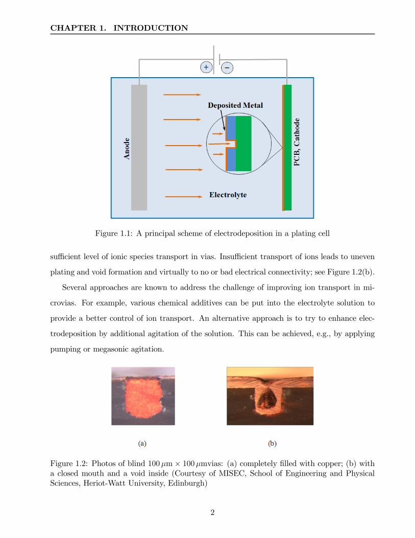
suffi cient level of ionic species transport in vias. Insuffi cient transport of ions leads to uneven
plating and void formation and virtually to no or bad electrical connectivity; see Figure 1.2(b).
Several approaches are known to address the challenge of improving ion transport in mi-
crovias. For example, various chemical additives can be put into the electrolyte solution to
provide a better control of ion transport. An alternative approach is to try to enhance elec-
trodeposition by additional agitation of the solution. This can be achieved, e.g., by applying
pumping or megasonic agitation.
Figure 1.2: Photos of blind 100µm× 100µmvias: (a) completely filled with copper; (b) witha closed mouth and a void inside (Courtesy of MISEC, School of Engineering and PhysicalSciences, Heriot-Watt University, Edinburgh)
2

CHAPTER 1. INTRODUCTION
This thesis is devoted to the study of possible enhancement of electrodeposition in microvias
by an additional ordinary flow and/or by an acoustically induced flow, in particular, by acoustic
streaming, which is understood as stream-like non-periodic movements in a liquid media due
to megasonic agitation.
Methodologically, the thesis is focused on numerical modelling of the relevant physical
processes. The problem area and the methodology determine the main features of the thesis:
Multi-Physics: we deal with at least three physical processes: electrodeposition, fluid flow
and acoustic streaming and their interactions;
Multi-Scale: we distinguish between the phenomena that occur in the whole plating cell (the
macro level) and in a microvias (the micro level) and present general methodologies that
link the macro and micro models together;
Multi-Tool: in our numerical experiments we rely on several pieces of software that are
capable of handling numerical models for various physical processes; the used software
includes PHYSICA, COMSOL Multiphysics and PHOENICS.
For analysis and interpretation of the numerical results we use various techniques, including
statistical methods and Design of Experiments; the latter methods use the software called
Visual DOC.
This project has been conducted in collaboration with Heriot-Watt University and Merlin
Circuit Technology Ltd. Colleagues from these establishments have suppled the results of
practical experiments and other real-life data needed for verification of the computational
models.
1.1 Aims and Objectives
The goals of this research are:
Goal 1: Develop numerical models for ion transport and electrodeposition in microvias, under
basic and enhanced conditions;
3

CHAPTER 1. INTRODUCTION
Goal 2: Use results from modelling to determine whether better quality fillings of microvias
can be achieved under enhanced forms of electrodeposition.
The following objectives form the pathway to achieving these goals:
Objective 1: Review and document state of the art in modelling electrodeposition processes
for microvia fabrications.
This objective is addressed in Chapter 2 and 5.
Objective 2: Develop a numerical model for basic electrodeposition, driven by diffusion and
electromigration. Identify an approach to predicting evolution of the electrodeposition
interface.
This objective is addressed in Chapter 5.
Objective 3: Use the developed model and established metrics to predict an impact of dif-
ferent process parameters on the filling quality in microvias for basic electrodeposition.
This objective is addressed in Chapter 5.
Objective 4: Develop a multi-scale approach to model the influence of fluid flow on quality
of electrodeposition. This involves coupling macro models (the plating cell level) with
micro models (the microvia level) for flow behaviour. Demonstrate the approach with
industry examples for standard plating cells equipped with pumps.
This objective is addressed in Chapter 6.
Objective 5: Review and document mathematical models for acoustic streaming. Identify a
suitable approach to combine with above multi-scale models.
This objective is addressed in Chapters 3 and 7.
Objective 6: Assess the impact of acoustic streaming (due to megasonic agitation from trans-
ducers placed in the plating cell) on the quality of a fabricated microvia.
This objective is addressed in Chapter 7.
4

CHAPTER 1. INTRODUCTION
1.2 Overview of the Thesis
The remainder of the thesis is organised as follows. Chapters 2—4 provide the reviews of
mathematical models of electrodeposition, of acoustic streaming, and of the associated software
tools. Notice that the literature reviews on numerical modelling of electrodeposition, fluid
flow and acoustic streaming are included as sections into the corresponding chapters; see
Sections 5.1, 6.2 and 7.1, respectively.
Chapter 2 describes the process of electrodeposition and its role in the manufacturing
of microelectronic devices. We present the corresponding mathematical models, challenges of
basic electrodeposition, quantitative measures of its quality and discuss possible ways of its
enhancement. The material of this chapter is related to Objective 1.
Chapter 3 gives a detailed review of existing literature on mathematical models of acoustic
streaming, including the classification of acoustic streaming, the method of successive approx-
imation for computing components of the field variables, and solutions for various geometric
configurations. Applications of acoustic streaming to various areas are also surveyed. This
section addresses Objective 5.
The main software tools used in this research are briefly discussed in Chapter 4.
Numerical modelling of basic electrodeposition is studied in Chapter 5. It gives an
overview of the existing approaches and presents a detailed description the Explicit Interface
Tracking Method (EITM), which plays the crucial role in reaching the goals of the project. The
method is validated against real-life measurements and known benchmarks. The experiments
show that in general under the conditions of basic electrodeposition it is unlikely to achieve a
good quality filling. The material of this chapter is related to Objectives 1, 2 and 3.
Chapter 6 addresses the flow phenomena that occur in a plating cell, at both macro and
micro levels. A general multi-scale methodology for numerical modelling of these phenomena
is developed. It is shown how a cell’s design affects ion transport in the whole bath and in
a via. Based on the results of numerical experiments and parametric studies, the conditions
that guarantee a better ion transport are derived. This chapter addresses Objective 4.
Numerical modelling of acoustically induced phenomena, such as acoustic streaming, is
the topic of Chapter 7. A general multi-scale methodology for numerical modelling of
5

CHAPTER 1. INTRODUCTION
Figure 1.3: The structure of the thesis
these phenomena is presented, the factors that may affect electrodeposition are analysed. For
the through vias, a combined numerical model that integrates electrodeposition and acoustic
streaming in the via is described. In accordance with Objective 6, the chapter gives clear
answers to which extend acoustic streaming can be useful for enhancing electrodeposition.
Chapter 8 gives an overview of made contributions and derived conclusions, as well as
outlines topics for future research.
The connections between the chapters, other than the introduction and conclusion, are
shown in Figure 1.3.
1.3 Contributions
In this section, we list what can be seen as major achievements of the project and their possible
implications.
• The development and implementation of the EITM, as well as numerical experiments
with the method, have contributed to a better understanding of electrodeposition in
microvias, in the basic and enhanced forms.
• The designed methodology of handling flow phenomena in a plating cell not only allows
us to assess ion transport at both macro and micro levels, but also results into recom-
6

CHAPTER 1. INTRODUCTION
mendations regarding a possible design of the cell that provides conditions favourable
for electrodeposition in microstructures.
• The designed methodology of handling acoustic streaming in a plating cell shows that at
the macro level acoustic streaming provides better ion transport than an ordinary flow.
• At the micro level, it has been demonstrated that acoustic streaming inside microstruc-
tures has an negligible effect on the quality of electrodeposition. Thus, if megasonic
agitation enhances electrodeposition, this is achieved not due to acoustic streaming in
microvias but due to other accompanying phenomena.
The material of this thesis has been disseminated in the following publications:
1. Kaufmann J., Desmulliez M. P.Y., Tian Y., Price D., Hughes M., Strusevitch N., Bailey
C., Liu C. and Hutt D. Megasonic agitation for enhanced electrodeposition of copper.
Microsystem Technologies, 2009, 15 (8), 1245—1254.
2. Strusevich N., Hughes M., Bailey C. and Djambazov G. Numerical modelling of elec-
trodeposition phenomena. Proceedings of 2nd Electronics System-Integration Technology
Conference, ESTC 2008, Greenwich, UK, 2008, 281—286.
3. Kaufmann J., Desmulliez M.P.Y., Price D., Hughes M., Strusevich N. and Bailey C.
Influence of megasonic agitation on the electrodeposition of high aspect ratio blind vias.
Proceedings of 2nd Electronics System-Integration Technology Conference, ESTC 2008,
Greenwich, UK, 2008, 1235—1240.
4. Hughes M., Strusevich N., Bailey C., McManus K., Kaufmann J., Flynn D. and Desmul-
liez M.P.Y. Numerical algorithms for modelling electrodeposition: tracking the deposi-
tion front under forced convection from megasonic agitation. International Journal for
Numerical Methods in Fluids, 2010: 64(3), 237—268.
5. Costello S., Flynn D., Kay R.W., Desmulliez M.P.Y., Strusevich N., Patel M.K., Bailey
C., Jones A.C., Bennet M., Price D., Habeshaw R., Demore C. and Cochran S. Elec-
trodeposition of copper into PCB vias under megasonic agitation. Proceedings of 22nd
7

CHAPTER 1. INTRODUCTION
Micromechanics and Microsystems Technology Europe Workshop, MME 2011, Toens-
berg, Norway, 2011.
6. Costello S., Strusevich N., Patel M.K., Bailey C., Flynn D., Kay R.W., Price D., Bennett
M., Jones A.C., Habeshaw R., Demore C., Cochran S. and Desmulliez M.P.Y. Charac-
terisation of ion transportation during electroplating of high aspect ratio microvias using
megasonic agitation. Proceedings of EMPC-2011 - 18th European Microelectronics and
Packaging Conference, 2011, 233—239.
7. Costello S., Strusevich N., Flynn D., Kay R.W., Patel M.K., Bailey C., Price D., Bennet
M., Jones A.C. and Desmulliez M.P.Y. Electrodeposition of copper into high aspect
ratio PCB micro-via using megasonic agitation, Proceedings of DTIP 2012, Symposium
on Design, Test, Integration & Packaging of MEMS/MOEMS, Cannes, France, April
2012.
8. Costello S., Strusevich N., Flynn D., Kay R.W., Patel M.K., Bailey C., Price D., Bennet
M., Jones A.C. and Desmulliez M.P.Y. Electrodeposition of copper into high aspect
ratio PCB micro-via using megasonic agitation, Microsystem Technologies, 2013: 19(6),
783—790.
9. Strusevich N., Patel M. and Bailey C. Parametric modeling study of basic electrodepo-
sition in microvias, Proceedings of EMAP 2012, Hong Kong, December 2012, 145—149.
10. Strusevich N., Bailey C., Costello S., Patel M. and Desmulliez M.P.Y. Numerical mod-
eling of electroplating process for microvia fabrication, Proceedings of EuroSimE 2013,
Wroclaw, Poland, April 2013.
8

Chapter 2
Electrodeposition in Electronics:Theory and Practice
In this chapter, we overview the process of electrodeposition and its role in the manufacturing
of microelectronic devices. The mathematical models of electrodeposition are presented by
formulating the corresponding governing equations. We demonstrate drawbacks of electrode-
position, if implemented in a basic form, and discuss possible ways of its enhancement with
a purpose of improving the quality of the resulting filling in small vias. The material of this
chapter is related to Objective 1.
2.1 Copper Electrodeposition in Manufacturing of Elec-tronic Devices
Microelectronics has major influence on many aspects of the modern life. Computers and
mobile phones, cars and airplanes, games and medical devices all contain sophisticated micro-
processors responsible for their control. Microelectronics can be defined as a part of electronic
technology that deals with miniaturised electronic components assembled in an extremely
small and compact form. Various semiconductor components, including resistors, capacitors,
transistors, integrated circuits, etc. allow fabrication of numerous microelectronic products
of any sizes and forms. There is a need for fast and reliable design and development of new
microelectronic products that are smaller, more useful, more user friendly, faster, and cheaper
for the consumer. Microelectronic industry and associated research and development activi-
ties have become one of the main sectors of the world economy. On February 6, 2012, The
9

CHAPTER 2. ELECTRODEPOSITION IN ELECTRONICS
Figure 2.1: Printed Circuit Boards
Semiconductor Industry Association (SIA), announced that worldwide semiconductor sales
for 2011 reached a record $299.5 billion, an increase of 0.4 percent compared to 2010; see
http://www.sia-online.org.
Without going into details of the manufacturing processes in microelectronic industry,
below we briefly overview those aspects that are essential for this project.
Semiconductor devices are electronic components that exploit the electronic properties of
semiconductor materials, such as silicon, germanium, and gallium arsenide. Most modern
semiconductor devices are integrated circuits (ICs) and packages that combine ICs with other
electronic components. When making a device, its electronic parts must be assembled and
appropriately connected. A device may consist of many components interconnected on a single
substrate (a PCB) that mechanically supports and electrically connects electronic components.
As a rule, a PCB’s substrate is made of glass fiber reinforced with epoxy resin, with a copper
foil bonded on to one or both sides. Only desired copper traces are left, by removing unwanted
copper, e.g., by photoetching. Double-sided boards or multi-layer boards use through holes
to connect traces on the opposite sides of the substrate. See Figure 2.1 for images of typical
PCBs.
One of the recognised trends of modern microelectronics is multi-layer (or 3D) packaging
of the components placed on several PCBs. This leads to miniaturised devices with a high-
speed performance, mainly due to short interconnects and reduced signal delays. The research
and development in the area of interconnection and packaging is motivated by increasing
requirements on performance and reliability of electronic devices and systems.
10

CHAPTER 2. ELECTRODEPOSITION IN ELECTRONICS
1 2
3
Figure 2.2: Types of vias: (1) - through, (2) - blind (trench), (3) - buried
The connection between different layers is provided by the so-called vertical interconnect
access (via), which is a vertical hole filled with metal to facilitate conductivity. We will
distinguish between
• open vias (also known as through vias);
• blind vias (known as trenches) exposed on one side of the board only;
• buried vias that connects internal layers but are not exposed on either side of the board.
See Figure 2.2.
There are several ways to provide interconnection in a multi-layer device. In this study, we
mainly address the most commonly used approach based on filling vias with metal (copper) by
electrodeposition. An alternative approach is to fill vias with a conductive paste. In the case
of the buried vias, conductive bumps are formed following by stacking the layers together.
According to Kondo et al. [85] and Beika et al. [13], a typical 3D packaging process that
involves deposition of copper as a filling metal into a via may include the following steps:
1. formation of vias by etching or drilling;
2. formation of a silicon insulating layer;
3. deposition of a barrier layer and a copper seed layer;
4. electrodeposition of copper inside the via;
5. formation of bumps followed by polishing;
6. multi-layer stacking of chips connected through the vias.
11

CHAPTER 2. ELECTRODEPOSITION IN ELECTRONICS
Steps 2-4 listed above are responsible for providing electrical interconnection. To make sure
that parts of the electronic device are properly connected by vias, the vias have to be filled
with a conductive metal, e.g., copper. A copper layer cannot be deposited directly onto the
substrate, since diffusion of copper onto surrounding materials would degrade their properties.
A thin barrier layer, consisting of tantalum, titanium or their nitrides is applied first; see
Step 3. Since electroplated copper does not adhere to the barrier materials, a thin copper seed
is deposited first on top of the barrier layer, typically by physical vapor deposition. After that
electrodeposition of copper can start, as stated in Step 4.
Deposition is one of the steps of the production activity, and is usually understood as any
process that grows, coats, or otherwise transfers a material onto the substrate. The techniques
of deposition known in industry include:
• physical vapor deposition
• chemical vapor deposition
• atomic layer deposition
• molecular beam epitaxy
• electrochemical deposition (ED).
In this study, we are mainly concerned with the last type of deposition, ED, and its applica-
tion to making conductive interconnects. Compared to other approaches, ED offers significant
cost, reliability and environmental advantages over the previously used evaporation technology
and is applicable to a wide range of sizes of vias of rather small diameter, even less that 1µm.
In accordance with modern manufacturing trends, in our models the metal to be deposited
into vias will be copper. An alternative to copper could be aluminium and its alloys, which
have had certain advantages, especially in manufacturing earlier devices in which the issue
of miniaturisation has been less essential. Aluminium alloys possess a low electric resistivity
and can be etched or patterned. They admit a low-cost fabrication process, and would easily
adhered to most dielectrics used as substrates.
12

CHAPTER 2. ELECTRODEPOSITION IN ELECTRONICS
According to Merchant et al. [105] and Suni et al. [156], the wide replacement of aluminium
with copper has become since 1997. With the growth of the number of layers in the 3D
packages, to guarantee their fast and reliable performance, a transition from aluminium to
copper has taken place. Copper makes a better choice since it is a better conductor than
aluminium, and therefore the ICs will have smaller metal components, and use less energy to
let the current flow through. Less metal also means a reduction in size of the device. As a
result, the time delays are reduced.
Another advantage of copper is its better resistance to electromigration; as estimated by
Pratt [130], copper has up to 100 times more resistance to electromigration failures than
aluminium. Recall that electromigration is the process of a metal conductor changing its shape
under the influence of an electric current. Small resistance to electromigration eventually leads
to the breaking of the conductor. The improvement in electromigration resistance allows higher
currents to flow through a copper conductor compared to an aluminium conductor of the same
size. Furthermore, copper has excellent thermal conductivity, twice than that of aluminium,
which improves cooling of circuit boards.
It is worth noticing, that ED can be performed near room temperature from water-based
electrolytes in a standard plating cell.
Still, using copper is not fully free from drawbacks, and the transition from aluminium
to copper has required significant developments in fabrication techniques, including entirely
different methods for patterning the metal. Copper diffuses very rapidly in silicon and conven-
tional dielectrics and that leads to inter-level and intra-level shorts. To reduce this undesirable
effect, encapsulated barrier layers are introduced; see Step 3 of the 3D packaging process above.
Unlike aluminium alloys, copper lines can not be easily patterned or etched, and a so-called
Damascene and a dual Damascene fabrication technique must be used [9], [165]. Besides, un-
like aluminum, copper does not form a selfpassivating oxide, so copper exposed at the top of
vias or trenches needs to be protected.
Electrodeposition in recessed microcavities and microtrenches forms the electroforming
part of the LIGA process, widely used in microelectronics. LIGA is the accepted acronym
for the German words for lithography, electroforming and molding. In a LIGA process, a
13

CHAPTER 2. ELECTRODEPOSITION IN ELECTRONICS
layer of photoresist is spread over a thin conducting seed layer and is then patterned by
lithographic techniques. Usually patterns are of micron or submicron dimensions and they act
as electroforming molds with a conducting base and insulating walls. A metal is deposited
on the patterned surface to produce a metallic microstructure that is negative in feature with
respect to the micromold. A LIGA process allows for the replication of the primary structure
in large quantities and low cost. See [65] for more details.
Further in this chapter, we formally explain the phenomenon of electrodeposition, describe
the factors that may affect its quality, and derive the main governing equations. The cor-
responding variables, their notation, physical meaning, units and, in some cases, values are
collected in Table 1.
2.2 Electrochemistry of Electrodeposition
Deposition or plating has been known as a technological process for many centuries; however,
before Alessandro Volta invented electrolytic deposition in 1800, the main form of deposition
had been electroless deposition also known as chemical or auto-catalytic plating. The latter
technique uses no external current flows and is based on several simultaneous reactions in an
aqueous solution.
Electrolytic deposition or simply electrodeposition (ED) is a process of producing a coating,
usually metallic, on a surface of a conductive object by the action of electric current. Below
we give necessarily technological details of the processes used in copper ED. A comprehensive
exposition of various aspects of metal ED can be found in [60].
The deposition of a metallic layer onto an object is achieved by putting a negative charge
on that object and immersing it into an electroplating cell (or a plating bath) filled with an
electrolyte solution. An illustration of an electroplating cell is shown in Figure 2.3.
The main components of the bath are:
• the negatively charged electrode, the cathode;
• the positively charged electrode, the anode;
• the power source;
14

CHAPTER 2. ELECTRODEPOSITION IN ELECTRONICS
Figure 2.3: A principal scheme of an electroplating cell
Figure 2.4: Electroplating baths: (a) an empty 25 l bath for laboratory experiments, courtesy ofThe Heriot-Watt University; (b) a filled industrial bath, courtesy of Merlin Circuit TechnologyLtd.
• a tank with an electrolyte solution.
Figure 2.4 shows the photographs of two electroplating cells used by the ASPECT project
partners.
The direction of current is defined as a movement of a positive charge, i.e., from plus to
minus. The electrodes are externally connected by wires via the electric power source. The
circuit is closed via the electrolysis bath filled with a conducting solution. The object to be
plated is the cathode of the circuit. The anode material can either be the metal to be deposited
or can be an inert material; however, in the latter case the solution is eventually depleted of
metal ions. A power source is either a battery or a rectifier that supplies a low voltage direct
current (DC).
15

CHAPTER 2. ELECTRODEPOSITION IN ELECTRONICS
An electrolyte is a liquid that contains mobile ions and can be produced either by melting
an ionic compound or by solvation or reaction of the compound with a solvent (such as water).
There are several electrolytes used for electrolytic copper deposition, but sulfate based systems
are most commonly used in PCB manufacturing due to their low cost, convenient operation
and safety. The electrolyte usually contains one or more dissolved metal salts. As described by
Lefebvre et al. [92], a widely used acid copper sulfate system consists of copper sulfate, sulfuric
acid, chloride ions and appropriate organic additives. Copper sulfate is the initial source of
copper ions in solution.
A popular electroplating technique begins from dissociation of a salt in water to positively
charged metal cations and negatively charged anions. A wire has to be attached to the object
(cathode) to be plated and to connect it with the negative pole of an external supply of direct
current. The anode is connected to the positive terminal of the power source. When the power
supply is switched on, electrons are directed into a path from the power supply to the cathode.
In the bath the electric current is carried by the positively charged copper ions towards the
cathode. This movement makes the metal ions in the bath to migrate towards extra electrons
that are located at or near the cathode surface. Finally, ions (cations) are removed from the
electrolyte and are reduced at the cathode to deposit in the metallic, zero charge state, by
gaining electrons. The reaction on the cathode can be written in the form
M+z + ze− => M,
where M+z is a metal ion with the positive charge of z units, e− is an electron and M is a
neutral, zero charge atom. In the case of copper deposition, the cathode reaction becomes
Cu+2 + 2e− => Cu.
During this reaction, the metallic copper is being deposited on the cathode, and the ions
of copper are being lost from the electrolyte. To overcome this depletion of ions, the copper
ions must be continuously provided to the electrolyte. There are two ways of doing this:
• via solid copper anodes;
• by replenishing the electrolyte with a solution containing dissolved ions.
16

CHAPTER 2. ELECTRODEPOSITION IN ELECTRONICS
The roles of other components of the electrolyte solution are as follows. Sulfuric acid serves
to improve the overall solution conductivity and to reduce anode and cathode polarisation.
Chloride ions also reduce polarization and additionally refine the deposit structure. When
copper anodes are used, chloride ions aid their corrosion, creating a uniform and adherent
film.
Various additives that are present in the electrolyte system are used to further refine deposit
characteristics. The copper sulfate system operated without additives typically yields deposit
of poor physical properties. Organic additives are employed to improve grain refinement,
throwing power, leveling of deposit. Generally there are three basic types of additives used
in acid copper plating: suppressors, accelerators and levelers. We discuss the roles of the
additives in more detail in Section 2.5.
2.3 Mass Transfer During Electrodeposition
Presenting the material of this section, we mainly follow the monographs [84] and [133].
Two processes are mainly responsible for ion transfer during electrodeposition:
• diffusion which is caused by the difference in concentration of cupric ions, i.e., the ions
move from the areas with a larger concentration towards regions with a lower concentra-
tion;
• migration which is caused by the electric field, i.e., positively charged cupric ions move
towards the negatively charged cathode.
Electrodeposition is multiphysical in nature, since it involves ionic concentration changes,
deposited layer evolution, electric current, fluid flow, heat transfer and other physical phenom-
ena. In microelectronic applications, ED is also multyscale, because the chemical reactions at
the metal (copper) surface represent a length scale of nanometers (surface roughness) and a
time scale of nanoseconds to microseconds, while the diffusion and migration processes in the
electrolyte solution occur at the micrometer to millimeter length scale.
Speed of diffusive mass transfer is determined by the diffusivity of cupric ions in the elec-
trolyte. Diffusivity of cupric ions in the electrolyte solution is denoted by D, see Table 1, which
17

CHAPTER 2. ELECTRODEPOSITION IN ELECTRONICS
is considered homogenous, i.e., the same in every direction. The amount of ions travelling over
a certain domain in a certain time determines the diffusion-dependent behavior of the species
in question. This amount, known as the diffusive material flux , is denoted by NDiff and is
given by Fick’s First Law of Diffusion
NDiff = −D ∇C. (2.1)
Due to the potential difference between the cathode and the anode, the whole electrolyte
bath is under the influence of an electric field. The field induces a force on the electrically
charged particles in the bath, causing them to start migrating towards the direction of less
potential difference between the particles charge and the field.
The speed of migrative mass transfer of cupric ions is determined by their mobility or ionic
mobility defined by the Einstein relation as DRT, where R is the universal gas constant and T
is temperature, see Table 1. Electrolysis always includes charge transfer; in our case, charge
is transferred by the Cu2+ ions. The material flux of the charge carriers (i.e., of cupric ions)
is denoted NMigr and is given by the relation
NMigr = −zFDRT
C ∇φ, (2.2)
The two factors that affect the mass transfer can be combined together to determine the
mass flux by the equation
N = NDiff +NMigr = −D ∇C − zFDRT
C ∇φ, (2.3)
known as the Nerst-Planck equation.
Differentiating the right-hand side of (2.3) with respect to the spacial variables will deter-
mine the rate of change of concentration, i.e.,
∂C
∂t= ∇ · (−D ∇C)−∇ ·
(zFD
RTC ∇φ
)(2.4)
= −D∇2C − zFDRT∇ · (C ∇φ) .
The latter equation serves as the basis of the numerical models described later in this
chapter.
18

CHAPTER 2. ELECTRODEPOSITION IN ELECTRONICS
2.4 Current Density Regimes
Current density i is the amperage of the electrodeposition current divided by the area of the
deposition surface. The value of the current density strongly effects the deposition rate and
plating quality. As the deposition process evolves in time, the deposition rate, that evaluates
how much metal, is deposited during each time step is described by Faraday’s Law given below
v =Ωi
zF· n, (2.5)
where v is the deposition rate (growth velocity) and Ω is the atomic volume of copper. The
higher the current density, the faster the deposition rate will be, although plating quality and
adhesion of a metallic layer may become lower when the deposition rate is too high.
Dukovic [45], Low et al. [101] and Byrne et al. [23] consider three types of current distrib-
ution models depending on the characteristics of the cathode boundary.
For a primary current distribution , the surface potential of the electrode is usually set
equal to the potential of the solution adjacent to the electrode. In this case, the electrolyte
resistance is much higher than the resistance of the interface due to the electrode kinetics.
The primary current distribution assumes that both the charge transfer and mass transport
conditions are negligible. The main aspect that determines the current distribution is the
ohmic resistance and the current density i at the electrolyte-electrode interface determined
from Ohm’s Law
i = k∇φ · n. (2.6)
For a secondary current distribution, the concentration of ions is very high and the con-
centration gradient is negligible. In this case, the electrochemical reaction is dependent on the
charge transfer only. The concentration of ions may be assumed similar at the cathode surface
and in electrolyte. Under these conditions, the current density can be related to the overpo-
tential that is denoted by η and is defined as the potential difference between the electrode
and the electrolyte adjacent to the electrode, i.e.
η = φelectrode − φelectrolyte.
19

CHAPTER 2. ELECTRODEPOSITION IN ELECTRONICS
The magnitude of the current density can be calculated using Tafel approximation
i = −i0 exp
(η
bc
), (2.7)
where bc is the Tafel slope that provides information about the mechanism of the reaction and
measured experimentally. The boundary conditions for the secondary current distribution are
given by (2.6).
The tertiary current distribution regime is considered when the concentration gradient is
significant and the electrochemical reaction depends on both the charge transfer and mass
transport. The current density is a function of the surface overpotential and ion concentration
and can be found using the Butler-Volmer equation for the cathodic reaction, which in the
general form can be written as
i = i0
[exp
(αanzFη
RT
)− C int
C∞exp
(−αcathzFη
RT
)], (2.8)
where i0 is the exchange current density, C int is the molar concentration at the metal-
lic/electrolyte interface, i.e., in the vicinity of the cathode, and C∞ is the concentration in
the far field. Here αan and αcath are the (dimensionless) transfer coeffi cients for the anode and
for the cathode, respectively. In this study, we, as most of the authors, assume that αan = 1.5
and αcath = 0.5.
Mass and charge concentration requires that the following flux conditions should be satisfied
at the interface
i = −k ∇φ · n = σ∇φ · n = zFD ∇C · n.
The secondary current distribution regime can be seen as a simplified version of the tertiary
regime if the ion concentration variation is ignored.
Malyshev et al. [103] stress that under the primary current distribution the electrolyte
ohmic resistance acts as the main controlling parameter, while the secondary current dis-
tribution deals with the mixed ohmic and electrode kinetics control. The tertiary current
distribution additionally allows the mass transport control.
Other types of current distribution are also known. For example, Chivilikhin et al. [27]
along with the Tafel approximation (2.7) study simpler linear and linearised models of the
20

CHAPTER 2. ELECTRODEPOSITION IN ELECTRONICS
current distribution. Ritter et al.[143] include in their classification also the case of diffusion-
limited current distribution. The metal deposition rate is determined directly from the flux of
ions to the electrode surface. A limiting current can be observed as the ion concentration at
the surface approaches zero and electric field effects are ignored. At the interface, the metal
ion concentration C int is set to zero and the current density in this case is calculated as
iDL = zFD (∇C · n) |Cint=0.
In this work, we mainly focus on the ED models under the tertiary current distribution,
with exact relations given in Section 5.2.
2.5 Challenges of Electrodeposition in Small Vias
In this section, we discuss the issues of obtaining good quality fillings of vias and point out
several approaches that might improve that quality.
As stated earlier, one of the current trends of modern microelectronics is achieving further
miniaturisation of devices. This can be done by increasing the density of vias on the board,
thereby reducing their diameters and increasing the aspect ratio, to become higher than 10:1.
However, filling high aspect ratio (HAR) microvias presents considerable technological prob-
lems.
2.5.1 Qualitative Characteristics of Electrodeposition
A microvia can be seen as electroplated successfully if it is completely full (leaving no internal
voids) but not excessively full (leaving a fairly smooth surface for the next layer to be staked).
Such a via will guarantee optimal electric conductivity.
Thus, to produce a high quality filling of a via, actions should be taken to avoid two
undesirable effects:
• overplating, i.e., crowding formed at the mouth of the via, and
• underplating, i.e., unacceptably thin layers at the bottom of the via.
21

CHAPTER 2. ELECTRODEPOSITION IN ELECTRONICS
Figure 2.5: Unwanted effects during ED in vias (overplating at the mouth and underplatingat the bottom)
These unwanted phenomena are shown in Figure 2.5. If not properly avoided, these defects
will create various reliability problems. For example, the presence of a void may totally
interrupt the circuit.
To a very large extend, the quality of filling is determined by the relative deposition rates in
various parts of the via. Figure 2.6 illustrates the three types of deposition for a small trench.
In the case of superconformal deposition, higher deposition rates are achieved at the bottom of
vias than on their sides. For subconformal deposition the relation between the two rates is the
opposite and for conformal deposition the rates are essentially equal. For copper, a natural
way is to be deposited subconformally; however, in this case both overplating and underplating
are likely to occur. Indeed, the protrusive parts of the region (e.g., sharp corners) will attract
higher cupric ion concentration, and therefore a larger current density and a thicker deposited
layer than the hidden parts of the region.
Thus, an effort should be made to achieve a superconformal filling, or at least conformal
filling. If the filling is conformal, the via is fully filled, but a seam is formed in the middle of
the via. The most preferable is superformal deposition that produces a void-free and seamless
filling.
2.5.2 Quantitative Characteristics of Electrodeposition
To provide the quantitative metrics of the ED quality, several measures are known [92, 93, 50].
Suppose that the measurement of the (partially) filled via are taken as shown in Figure 2.7,
where
22

CHAPTER 2. ELECTRODEPOSITION IN ELECTRONICS
Figure 2.6: Types of deposition: (a) subconformal leading to void formation; (b) conformalleading to seam formation; (c) superconformal leading to a defect-free filling
• H is the via height;
• d is the radius (i.e., H2dis the aspect ratio);
• h1 is the thickness of the deposited layer on the board;
• h2 is the thickness of the deposited layer in the middle of the via height;
• h3 is the thickness of the deposited layer at the centre of the bottom of the via.
Table 2.1 shows several metrics for measuring the quality of ED in vias.
Name Notation FormulaDimple Depth DD H − h3
Relative Deposition Thickness RDT h3/h1
Via Fill V F 1− (d−h2)2
d2(H−h3)
H
Table 2.1: Performance metrics for ED in vias
The introduced metrics admit the following meaningful interpretations:
• Dimple Depth DD measures the height of the unfilled part of the trench;
23

CHAPTER 2. ELECTRODEPOSITION IN ELECTRONICS
Figure 2.7: Via filling measurements
• Relative Deposition Thickness RDT compares the growth of the deposition levels in the
bottom part of the trench (h3) and at the mouth, on the PCB surface (h1);
• Via Fill V F is the fraction of the via volume filled with metal.
For good quality fillings, DD approaches 0, while V F approaches 1 and RDT takes values
larger than or equal to 1.
We use these metrics in Sections 5.5 and 5.7 for a purpose of validation of our approach to
numerical modelling of ED.
2.5.3 Achieving Good Quality of Deposition
To achieve a superconformal filling, the techniques are needed to control the deposition rates
in various parts of the via. The deposition rate in vias depends on both
• ion transport, and
• surface reaction kinetics.
We call electrodeposition basic, if the electrolyte is just a water solution of copper sulfate.
Basic electrodeposition allows a clear understanding of the phenomena and is therefore a useful
model for theoretical studies; in fact, the whole chapter of this thesis is devoted to numerical
modelling of basic electrodeposition. However, basic electrodeposition is known not to be able
to guarantee high quality fillings of HAR vias. The reason of this underperformance is that
the ion transport is mainly provided by ion diffusion and migration in the electrolyte solution.
24

CHAPTER 2. ELECTRODEPOSITION IN ELECTRONICS
Deposition rates are therefore limited to the speed of diffusion and migration processes. With
increasing via depth, the path length for diffusion becomes longer, reducing the rate of trans-
port relative to the deposition rate. The deposition rates become slower in lower parts of the
via which results into an undesired subconformal filling.
There are several ways of achieving a better deposition performance by controlling the
reaction kinetics and/or enhancing the ion transport.
• Choosing the via profile
• Controlling a current density regime
• Finding an optimal composition of the electrolyte
• Using double anodes
• Electrolyte solution agitation
Choosing the via profile is a fairly straightforward but effective approach. As demon-
strated by numerous experiments, vias of a barrel shape are harder to fill compared to those
of rectangular profile, and the best results are observed for the tapered vias [92].
Increasing current density will improve the ion transport; however, this does not neces-
sarily lead to better values of the quality metrics (see Table 2.1). As pointed out by Tsai et al.
[162], the increase of current density leads to a growth of the consumption rate of the ions in
the via. This produces a discontinuity of the metal ion transportation in the bulk electrolyte
and non-uniform structure of the deposited metal, which also may contain gas bubbles. On
the other hand, reducing the current density would increase the time required to complete
the electroforming process. The influence of the current density regime becomes more evident
as via depth increases, i.e., the aspect ratio grows. In Section 5.7, we report on a numerical
experiments that use the current density as one of the design parameters.
As stated in Section 2.1, in practice a solution used as the electrolyte is a rather complex
mix of salts, acids and various additives. Studies of the composition of the electrolyte is
one of the most active directions of research in the area. Generally there are three basic types
25

CHAPTER 2. ELECTRODEPOSITION IN ELECTRONICS
of additives used in acid copper plating: suppressors, accelerators and levelers. Following [92],
[165] and [130], we briefly describe the functioning of these additives.
Suppressors/inhibitors are large-sized polymers such as polyethylene glycol. These mole-
cules with high molecular weight diffuse relatively slowly, but they are very rapidly adsorbed
into the surface of the cathode. They work along with chloride ions contained in the solution
to suppress the plating rate due to formation of an organic film that blocks the copper ions
access to the surface. The result is strong inhibition of the deposition reaction.
Accelerators are sulphur molecules. Due to their small size they diffuse fast, but are ad-
sorbed slowly in the copper. Accelerators on their own do not increase the deposition rate.
They provide a localised increase in deposition rate, typically at the bottom of the via, and
reduce the effect of the inhibitors on slowing down the deposition process.
Levelers are typically nitrogen-based aromatic compounds. They are used to make the
surface of the deposited metal smoother. Their molecules are smaller than those of suppressors
and their presence leads to preferential metal deposition into valleys of the surface, rather than
onto peaks.
A fairly high concentration of suppressors and levellers at the mouth decreases the depo-
sition rate in that area, thereby preventing a crowding effect [169]. According to the experi-
mental results on electrodeposition of copper in microvias presented by Lühn et al. [102], the
use of levelers increases the overpotential either at the mouth of the via or at protrusions on
the surface to prevent overplating. On the other hand, due to a lower concentration of these
additives inside the via, the local deposition rate is mainly affected by the accelerators and is
higher than at the mouth. As a result a more uniform, superconformal filling is produced. See
[9], [86] and [173] for discussion and experimental results.
Even from this concise description it can be seen that the interaction between different types
of additives is a complex process, so that the monitoring, control and replenishment of additives
in the electrolyte is a diffi cult task. Besides, the use of additives has additional drawbacks.
Suni et al. [156] mention that additives may remain in the copper deposit and that may
cause defects. Moreover, accelerators continue acting after the vias are filled, allowing bumps
to form, so that the subsequent planarisation may become diffi cult. Hence, electrodeposition
26

CHAPTER 2. ELECTRODEPOSITION IN ELECTRONICS
techniques that operate with additive-free electrolyte are highly desirable.
Jang et al. [74] propose to insert double anodes and a penetrating jig between them
into the electrolyte. They report that their method improves the deposition rate and allows a
void-free filling micro-vias of a diameter of 40µm and aspect ratios of 6.25:1 and 10:1.
Electrolyte solution agitation (ESA) provides methods that guarantee accelerated
movement of the ions by generating a flow at the approach to and inside of the via. In this
thesis, the ED techniques based on ESA are called enhanced electrodeposition.
This project is aimed at making a further contribution in namely this direction by study-
ing generalised numerical models of enhanced electrodeposition. We focus on two types of
enhancement that lead to an improved ion transport and eventually to a better quality plat-
ing:
Forced Flow: This approach is based on generating an additional flow of the electrolyte in
the plating cell;
Acoustic Streaming: This approach is based on the use of high frequency sound waves that
generate electrolytic flow deep into the vias and thereby replenish the supply of ionic
species.
We have chosen these two approaches, since due to a relatively large longitudinal dimension
of high AR vias, traditional methods for enhancing ion transportation in the electrolyte bath,
such as stirring, appear to be useless as shown by Tsai et al. [162]. The forced flow enhancement
can be achieved, by pumping, i.e., equipping the plating cell with a flow inlet; see Chapter 6.
Another way is to rotate the cathode, which generates an additional flow [63, 89]. A review
of the theory of acoustic steaming is presented in Chapter 3, and possibilities of its use for
electrodeposition are discussed in Chapter 7.
27

Chapter 3
Acoustic Streaming and ItsClassification
In this chapter, we discuss various theoretical aspects of acoustic streaming, present a classi-
fication of various types of that phenomena and illustrate it under different conditions. The
material of this chapter corresponds to Objective 5 of the thesis set in Section 1.1.
3.1 Phenomenon of Acoustic Streaming
Propagation of high-power sound waves in gas and liquid media often leads to stream-like non-
periodic movements. According to Lord Rayleigh [137], the term “acoustic streaming”(AS) is
used to describe the steady time-averaged unidirectional fluid flow that is induced in a liquid
or gas medium and is dominated by its fluctuating components. Less formally, Frampton
et al. [56] define AS as the creation of steady fluid velocity from acoustic, or oscillating,
velocities. This phenomenon has been extensively studied; still, as admitted in one of the
most recent surveys on this topic [15], “...despite a century of study initiated by Rayleigh,
acoustic streaming is far from understood”.
Propagation of sound can be viewed as flow of wave energy. When this flow is interrupted
either by the medium in which sound propagates or by an object in the medium, the sound
generates a force to push it in the direction of propagation. The study of AS belongs to the
area of Nonlinear Acoustics; this is because the vibrating amplitude dependence is due to the
nonlinear response of the medium in which the sound propagates, and not to the nonlinear
behavior of the sound source itself.
28

CHAPTER 3. ACOUSTIC STREAMING AND ITS CLASSIFICATION
The main reason for AS is the attenuation of the acoustic wave. The dominant attenuation
effects include viscous losses and rigid boundary interaction. Part of the wave energy lost
through attenuation is converted into energy for steady medium motion in the process of
sound propagation. The attenuation reduces the vibrating amplitude of the wave and hence
generates Reynolds stress distribution and drives the medium to form the AS [96]. Thus, the
motion generated in the medium due to vibration is essentially the sum of an oscillatory part
and a non-oscillatory time-independent steaming [145].
Different authors give various classifications of types of AS. However, most of the authors
accept the classification that is based on the scale of the medium motion and on the different
mechanisms by which it is generated [15, 72, 96, 100]. According to this classification, the
two types of AS are (i) streaming due to viscous losses and (ii) streaming due to boundary
interaction. See [106] and [142] for a comparative analysis of both types of AS.
The first type is often called Eckart type and is known as the “Quartz Wind”. It is
generated by the absorption of the sound wave in a viscous medium; in other words, it can be
attributed to the spatial attenuation of a wave in free space. Lee and Wang [91] provide the
following intuitive explanation of this phenomenon. Suppose that a medium particle vibrates
somewhat stronger when it is at the back rather than at the front of its equilibrium position
during an oscillation cycle because of the attenuation. Then on average the particle moves
forward a little bit over each cycle. These small displacements accumulated over many cycles
form AS. The scale of this motion is of a much larger order of magnitude compared to the
acoustic wavelength. The Eckart type of AS is associated with a high Reynolds number flow.
Although Eckart was not the first to observe the Quartz Wind, he was the first one who in
1948 analysed it mathematically in [46].
Boundary layer driven streaming occurs when the sound wave propagates close to a solid
surface. In this case, the non-slip boundary conditions lead to a considerable reduction of the
amplitude of the sound wave within a very thin layer next to the boundary, that is called
the acoustic boundary layer. This reduction of the amplitude is much larger than that in the
Eckart type streaming, and the associated Reynolds stresses and the magnitude of AS is also
much larger.
29

CHAPTER 3. ACOUSTIC STREAMING AND ITS CLASSIFICATION
Two kinds of boundary-layer streaming are distinguished: outer and inner. These two
types of streaming always occur together.
The study of boundary-layer outer streaming started with the theoretical work of Lord
Rayleigh [137]. Rayleigh analysed AS due to a standing wave present between parallel plates
and explained that the air motion was caused by a nonlinear second order effect. Rayleigh
focused his investigations on mean flows outside the boundary layer. The scale of boundary-
layer outer streaming, or the Rayleigh streaming, is comparable to the wavelength. It should
be noticed that the work of Rayleigh [137] was done in the XIX century. The phenomenon of
Quartz Wind was first observed in the 1920s, with the arrival of ultrasonic transducers, and
Eckart’s solution appeared in the 1940’s.
The study of inner boundary layer streaming was developed by Schlichting, who investi-
gated an incompressible oscillating flow over a flat plate, that moved through a liquid medium,
and calculated the two-dimensional streaming field inside the boundary layer [147]. Schlicht-
ing described how the boundary layer thickness depends on viscosity, density, wave length and
the outer flow velocity. His approach helps to describe vortex motion generated in a viscous
boundary layer on the surface of an object placed in a sound field. The scale of the Schlichting
streaming is much smaller than the wavelength.
Acoustic streaming is a nonlinear effect and is commonly treated as a second-order quantity
mathematically. One reason of being second-order is that the flow speed at any point in a sound
field is proportional to the square of the sound wave amplitude. While the medium outside
the layer vibrates irrotationally, the medium inside the layer is forced to vibrate rotationally
in order to conform to the non-slip condition on the wall. This second order rotational motion
forms a nonzero steady motion [91].
The classical work by Nyborg [122] is the most quoted in the area. He reviewed the theories
for calculating steady streaming associated with sound fields. He showed that acoustic steam-
ing can be understood by recognizing that the governing equations are similar to those for
incompressible flow of a fluid produced by an external force field. The theoretical approaches
are mainly based on successive approximations to solutions of nonlinear hydrodynamic equa-
tions, where the first and the second order solutions in each approximation must satisfy the
30

CHAPTER 3. ACOUSTIC STREAMING AND ITS CLASSIFICATION
boundary conditions. Accurate solutions exist only for the cases where the boundaries are
simple and where the specified velocity distributions on these boundaries are also simple.
Nyborg [122] provides a historic account on the developments in this direction. Frampton
et al. [56] study the Rayleigh acoustic streaming and demonstrate that the acoustic boundary
layer in a cylindrical tube filled with water is less than 1µm for a 1 MHz acoustic wave. Due
to the small thickness of the layer, its impact on the overall motion is more noticeable for a
channel of a smaller diameter.
Rudenko and Soluyan [145] use an analogy between AS and classical hydrodynamics and
come up with a classification of AS based on Reynolds number Re, which is known to char-
acterise a contribution of the non-linear terms into the streaming behavior. For small values
of Re, streaming can be viewed as slow and its parameters can be found by solving linear
or linearised equations. For large values of Re, non-linear hydrodynamic effects are essential
(except one-dimensional Eckart streaming due to the geometry of the problem). The types of
AS can be also distinguished e.g., by ratios of streaming velocity to oscillation velocity, or by
sound intensity. In particular, a possible classification presented in [145] is based on the rela-
tive values of heterogeneity of AS. In the case of this heterogeneity mainly affected by the size
L of the area in which streaming takes place, the streaming is called large-scale. Alternatively,
the most influential parameter can be either the wave length λ (for medium-scale streaming)
or the boundary layer thickness δ (for small-scale steaming). Since normally δ λ L, for
the corresponding Reynolds numbers we have that Reδ Reλ ReL, so that as the size of
heterogeneity decreases the non-linear effects tend to vanish, and to handle these streaming
types the linear equations become applicable.
Andres and Ingard [7] and [8] point out that the two types of flow associated with different
values of Reynolds numbers correspond to the two types of circulations, that are qualitatively
similar but reversed in direction. Their model includes a cylindrical obstacle, and the flow
pattern observed around this cylinder appears rotational, but for the case of a low Re its
direction is opposite to the direction of the flow that corresponds to a highRe.More specifically,
in the case with a low Re the steady streaming is directed towards the cylinder along the line
of sound propagation, while in the case of high Re the flow is directed away from the cylinder
31

CHAPTER 3. ACOUSTIC STREAMING AND ITS CLASSIFICATION
along this line.
In his review, Lighthill [96] also describes the theory of AS in both low and high Reynolds
number regimes.
In the remainder of this section, we discuss various features of AS as a physical phenomenon.
The corresponding variables, their notation, physical meaning, units and, in some cases, values
are collected in Table 2.
3.2 General Governing Equations
In this section, we present a brief development of the streaming equations. We mainly follow
Nyborg [122].
For sound waves in an unbounded fluid medium, equations of mass and momentum con-
servation can be written as
(i) Continuity equation∂ρ
∂t+∇ · (ρU) = 0. (3.1)
(ii) Equation of motion
∂(ρU)
∂t+U∇ · (ρU) + ρ(U · ∇)U = −∇P +
(4
3µ+ µb
)∇∇ ·U − µ∇×∇×U . (3.2)
According to Nyborg [120], the dynamic viscosity µ and kinematic viscosity µ/ρ can not
be treated as constants for gases in presence of sound waves, but for liquids they are usually
assumed to be constants. The terms on the right-hand side of equation (3.2) represent the
normal and tangential (shear) forces acting on the fluid element. The left-hand side terms
represent the force
f = ρ
(∂(U)
∂t+U · ∇)U
)that acts on the same fluid element due to stresses. It is easily checked that the left-hand
side(3.2) together with (3.1) yields the above expression for f.
It should be noted that the linearized form of equations (3.1) and (3.2), i.e. ignoring all
the second order small terms, collapses to give the wave equation.
32

CHAPTER 3. ACOUSTIC STREAMING AND ITS CLASSIFICATION
Figure 3.1: First and second order phenomena that accompany megasonic agitaiton
To derive the governing equations of acoustic streaming Nyborg [122] employs the method
of successive approximations. According to this method, the field variables (excess pressure,
density and velocity) are expressed as the sum of the first order small terms and the second
order small terms.
ρ− ρ0 = ρa + ρs + ... (3.3)
P − P0 = Pa + Ps + ...
U = U a +U s + ...
Here ρ0 and P0 are ambient values, they are assumed to be constant and uniform. The
first-order variables ρa, Pa and U a depend periodically on time with the angular frequency
ω. These variables describe the oscillating group of variables and represent sound field in the
linear approximation. The second-order variables ρs, Ps and U s include both the terms that
periodically depend on time with the doubled frequency 2ω and the terms which are time-
independent. The latter variables describe time independent contributions to excess pressure,
density and velocity. The second-order term U s is the streaming velocity we are looking for.
The first and second order phenomena are graphically illustrated in Figure 3.1, presented in
[145].
To determine the order of an expression that involves various components of ρ, P and U
it is convenient to put the subscript “a”to correspondence to 1 and the subscript “s”to 2.
Then for a triple (i, j, k), where i, j, k ∈ 0, 1, 2, the order of an expression that involves a
product of ρi, Pj and U k is equal to i+ j + k.
33

CHAPTER 3. ACOUSTIC STREAMING AND ITS CLASSIFICATION
To develop a method for finding U s, we start with substituting equations (3.3) into the
continuity equation (3.1) and the momentum equation (3.2), grouping the terms of the same
order and discarding the terms of an order greater than two. For instance, in the continuity
equation with respect to the variables of the first order we replace ρ by ρ1 and ρU by ρ0U a,
while in the case of the second order variables we replace ρ by ρs and ρU by ρ0U s + ρaU a.
The other equations are transformed similarly, and we obtain:
(i) Continuity equation
(a) first order terms:∂ρa∂t
+ ρ0∇ ·U a = 0 (3.4)
(b) second order terms:∂ρs∂t
+ ρ0∇ ·U s +∇ · (ρaU a) = 0. (3.5)
(ii) Equations of motion
(a) first order terms:
ρ0
∂U a
∂t= −∇Pa +
(4
3µ+ µb
)∇∇ ·U a − µ∇×∇×U a (3.6)
(b) second order terms:
ρ0
∂U s
∂t+∂(ρaU a)
∂t+U a∇ · (ρ0U a) + ρ0(U a∇) ·U a (3.7)
= −∇Ps +
(4
3µ+ µb
)∇∇ ·U s − µ∇×∇×U s.
Notice that in the case under consideration the streaming velocity will be much less than
the sound velocity in the medium, so that the medium can be treated as an incompressible
liquid, i.e., the density is constant, ρ = ρ0 = const, as in [145]. This implies that in (3.4) and
(3.5) all derivatives of ρ are zero. This results in
∇ ·U a = 0
and, therefore, in
∇ ·U s = 0. (3.8)
34

CHAPTER 3. ACOUSTIC STREAMING AND ITS CLASSIFICATION
The equations that govern the AS flow are deduced by taking the time average of (3.6) and
(3.7) of all first-order variables. Here and throughout time averaging is denoted by 〈〉. The
time averages of the first-order variables are equal to zero, because of their periodic nature,
i.e.,
〈Pa〉 =1
T
∫ T
0
Padt = 0, 〈U a〉 =1
T
∫ T
0
U adt = 0.
The averaging process eliminates all simple harmonic terms. The equation for the first-
order variables vanishes, while equation (3.7) reduces to
〈U a∇ · (ρ0U a) + ρ0(U a∇) ·U a〉 = −∇Ps + (4
3µ+ µb)∇∇ ·U s − µ∇×∇×U s, (3.9)
due to the fact that U s is time-independent.
The left-hand side of (3.9) is usually denoted by −F , i.e.,
−F = 〈U a∇ · (ρ0U a) + ρ0(U a∇) ·U a〉 (3.10)
and is called the driving force that accounts for the transfer of momentum from sound wave to
the fluid. Mathematically, F can be seen as the time average of the products of the harmonic
functions.
Recall that for a vector field V , the gradient of the divergence is equal to the divergence
of the gradient plus the curl of the curl, i.e.,
∇(∇ · V ) = ∇(∇V ) +∇× (∇× V ),
which implies that
∇× (∇× V ) = ∇(∇ · V )−∇(∇V ) = ∇(∇ · V )−∇2V .
Applying the latter formula to ∇×∇×U s from the right-hand side of (3.9), we obtain
∇×∇×U s = ∇(∇ ·U s)−∇2U s.
Substituting this and (3.8) into the right-hand side of (3.9), we obtain a stationary Stokes
equation of the form
∇Ps − µ∇2U s = F. (3.11)
35

CHAPTER 3. ACOUSTIC STREAMING AND ITS CLASSIFICATION
Therefore, the steady streaming motion of an incompressible viscous fluid subjected to
driving force F is governed by the pair of equations (3.8) and (3.11) with F defined by (3.10).
As pointed out by Nyborg [122], equation (3.11) does not contain the inertial terms and
resembles the equations of motion for forced slow viscous flows.
Thus, the following method can be used for finding the values of the second-order variables,
given the acoustic velocity U a.
Algorithm UPs (for computing U s and Ps)
Step 1: Given U a, compute F by (3.10).
Step 2: With the found value F and an appropriate boundary, solve (3.8) and (3.11) for U s
and Ps.
Algorithm UPs is generic, and captures the logic of computation of U s and Ps for various
types of acoustic waves and different boundary conditions, as demonstrated in the forthcoming
sections of this chapter.
3.3 Plane Travelling Wave in Unbounded Medium
Suppose the sound field is created as a result of vibration of an ultrasonic transducer in a
bath of a width H. An attenuated plane wave travels in the positive x− direction in a fluid
medium. The transducer of a radius R is placed at one end of the bath along its central line,
where H > 2R. The sound field can be approximated as a beam of width 2R that moves along
the central line towards the opposite end of the bath, see Figure 3.2. The distance between
the beam and a wall of the bath is denoted by y1 = (H − 2R) /2.
The first order velocity in this case has only x−component and is given by
Ua = Ae−αx cos(ωt− kx) (3.12)
for all points in the beam and Ua = 0 outside the beam [122].
Here
36

CHAPTER 3. ACOUSTIC STREAMING AND ITS CLASSIFICATION
Figure 3.2: Geometry of the bath with the driving force inside the beam
A is the source acoustic velocity,
A =
√I
ρ0c; (3.13)
ω is the angular frequency of the sound wave, ω = 2πf ;
α is the attenuation coeffi cient [122]
α =2µω2
3ρ0c3; (3.14)
k is the wave number, k = ωc.
The driving force F has also only an x− component that we will denote by Fx. Equation
(3.10) becomes
Fx = −2ρ0〈Ua∂Ua∂x〉.
Notice that∂Ua∂x
= Ae−αx (k sin (ωt− kx)− α cos (ωt− kx))
and
Ua∂Ua∂x
= A2e−2αx
(k
2sin 2 (ωt− kx)− α cos2 (ωt− kx)
).
Since 〈sin 2 (ωt− kx)〉 = 0 and 〈cos2 (ωt− kx)〉 = 12, we deduce
Fx = A2αρ0e−2αx. (3.15)
This constant force acts in the positive x−direction on all fluid in the region occupied by
the beam. Outside the beam Fx = 0.
37

CHAPTER 3. ACOUSTIC STREAMING AND ITS CLASSIFICATION
If αx 1 in the region of observation, then Fx is nearly constant and can be written as
Fx = A2αρ0. (3.16)
3.3.1 Open Ends
If the ends of the channel are open (or, equivalently, the boundary x = L represents the ideal
sound absorption), we assume that the pressure term∇P s is zero and equation (3.11) becomes
µ
(∂2Us∂y2
)= −Fx
A solution of this equation for the lower part of the channel for which 0 ≤ y ≤ H/2 is given
by
Us =
ρ0αA
2
2µ(H − 2y1) y for 0 < y ≤ y1,
ρ0αA2
2µ(Hy − y2 − y2
1) for y1 ≤ y < H/2.(3.17)
The solution for H/2 ≤ y ≤ H is obtained by substituting (H − y) for y.
3.3.2 Closed Ends
If the ends of the channel are closed, we have to solve equation (3.11), where pressure gradient
is nonzero. The solution Us is just the sum of the solution for the case with open ends and that
for ∇P s 6= 0 and Fx = 0. Hence, we add to the solution Us given in (3.17) a complementary
term Ucompl that is valid for 0 ≤ y ≤ H and given by
Ucompl =ρ0αA
2
2µ
[1− 6
(y1
H
)2
+ 4(y1
H
)3]y (y −H) .
The final solution becomes
Us =
ρ0αA
2
µRy + Ucompl for 0 < y ≤ y1,
ρ0αA2
2µ(Hy − y2 − y2
1) + Ucompl for y1 ≤ y < H/2.
When 0 < 2R/H < 1, a flow pattern is expected to be as shown in Figure 3.3. Flow along
the centre of the bath is in the direction of propagation of the sound beam. Due to the mass
conservation, return flow occurs in the outer part of the bath. Since the driving force Fx is
expressed in terms of the attenuation coeffi cient α, we can find the streaming velocity Us at
any given point in the bath as a function of α.
38

CHAPTER 3. ACOUSTIC STREAMING AND ITS CLASSIFICATION
Figure 3.3: Streaming velocity profile with direct flow inside the beam and return flow outsidethe beam
3.4 Beam Filling the Tube: Standing Waves
In this section, we consider the situation that 2R = H, i.e., when the beam fills the entire
cross-section of the bath, between two parallel walls (plates). It is assumed that a standing
wave is generated.
Rayleigh [137] was the first who provided an analysis of motion of a medium in the interior
and close to the wall considering the flow induced by standing waves between parallel walls. He
used a successive approximation technique which has become the dominant analytical tool since
then for studying the AS. Rayleigh treated the flow on the wall as incompressible. However, as
noted by Westervelt [174], the Rayleigh analysis assumes that the first order motion is nearly
solenoidal.
Rayleigh’s solution [138] for the first order velocities in axial (x−axis) and transverse
(y−axis) directions are given by
Uax = A cos kx[cosωt− e−βy cos(ωt− βy)]
Uay = −(
k√2β
)(A sin kx)
[cos(ωt− π
4
)− e−βy cos
(ωt− βy − π
4
)],
where it is assumed that k β.
It can be seen that the boundary condition at the wall is satisfied since Uax and Uay are
each equal to zero for y = 0.
Substituting these values into (3.10) we obtain that the y−component of F is negligible
39

CHAPTER 3. ACOUSTIC STREAMING AND ITS CLASSIFICATION
Figure 3.4: Function f(n) used in (3.19)
and that the x−component of the driving force is given by
Fx = F (v)x + F (b)
x ,
F (v)x = A2kρ0 sin (2kx) ,
F (b)x =
1
4A2kρ0 sin(2kx)(e−2βy − 3e−n cosn+ e−n sinn).
In this chapter, it is convenient to use the following notation
C = e−βy cos(βy), S = e−βy sin(βy). (3.18)
Following Nyborg [122], denote n = βy and
f(n) = e−2n − 3e−n cosn+ e−n sinn = e−2n − 3C + S.
Then F (b)x can be rewritten as
F (b)x =
1
4A2kρ0 sin(2kx)f(n). (3.19)
The behavior of f as a function of n is shown in Figure 3.4. The extreme values of f(n)
are −2 for n = 0 and 0.33 for n = 2. When n ≥ 5, the value of f(n) is essentially zero, and
the component F (b)x can be ignored.
Let us split the x−axis by the points N (node) and A (anti-node); see Figure 3.5. As x
changes from A to N the value of sin(2kx) remains non-negative, while as x changes from N
to A the value of sin(2kx) remains non-positive. Since k = 2πλ, we can conclude that the length
of each A−N segment and each N − A segment is λ/4. See [121] and [145] for details.
40

CHAPTER 3. ACOUSTIC STREAMING AND ITS CLASSIFICATION
Figure 3.5: Distribution of the components of the driving force
This implies that the component F (v)x does not lead to streaming. We derive that in the
layer that is closest to a wall (n < 1) the values of F (b)x are large in magnitude due to the value
of f(n) for n < 1. In each A−N segment the sign of F (b)x is negative (the positive sin(2kx) is
multiplied by the negative f(n)), and in each N − A segment the sign of F (b)x is positive (the
negative sin(2kx) is multiplied by the negative f(n)). On the other hand, as we move away
from the wall, the values of f(n) become fairly small positive numbers, and in those layers the
values of F (b)x are smaller in magnitude compared to the value in the closest layer, and also
have the opposite sign. See Figure 3.5.
Still, as mentioned by Nyborg [122], the effectiveness of forces applied at distance y from
the wall increases as y increases. This implies that the forces of a larger magnitude in the
closest layer will be suppressed collectively by the forces in more remote layers. As a result, in
each segment close to the wall a vortex will occur, in the direction that is determined by the
direction of F (b)x in the dominating remote layers.
Nyborg [121] stresses that this phenomenon is experimentally observed in the Kundt’s tube
and concludes that for the standing waves between parallel walls the net flow must be zero,
although in the case of the travelling wave, AS may result in a non-zero net mass transport.
The resulting solution for the axial and transverse components of the streaming velocity,
assuming that the y−coordinate is measured from the wall, is given by [122] as
Usx =A2
4csin(2kx)
[−e−2βy − 2C − 6S − 18
y
H
(1− y
H
)+ 3], (3.20)
Usy = −1
4
A2k
cβcos(2kx)
[1
2e−2βy + 4C + 2S + 3βy
(1− y
H
)(1− 2y
H
)− 9
2
]. (3.21)
In the case of outer streaming, the solution above can be simplified taking into account
41

CHAPTER 3. ACOUSTIC STREAMING AND ITS CLASSIFICATION
that for the region far enough from the boundary layer the inequality βy 1 holds, and the
corresponding components can be written as in [15] and [122]
Usx =3
8
A2
csin(2kx)
[1− 6
y
H
(1− y
H
)]Usy = −3
2
A2kH
ccos(2kx)
y
H
(1− y
H
)(1− 2y
H
).
The study of streaming inside the boundary layer, or inner streaming, was first developed
by Schlichting [147]. He assumed an incompressible oscillatory flow over a flat plate and calcu-
lated the two-dimensional streaming field inside the boundary layer. Based on the assumption
that for the streaming inside the boundary layer yH 1, the streaming velocity components
in (3.20) and (3.21) become
Usx =1
4
A2
csin(2kx)
[−1
2e−2βy − C − 3S +
3
2
]Usy = −1
4
A2k
cβcos(2kx)
[1
2e−2βy + 4C + 2S + 3βy − 9
2
].
Boluriaan and Morris [15] following Rudenko and Soluyan [145] give even simpler expression
for the velocity components for the inner streaming
Usx =1
4
A2
cβy (1− βy) sin(2kx)
Usy = −1
4
A2k
cβy2 cos(2kx).
The velocity patterns for outer and inner streaming are shown in Figure 3.6 (the bottom
half of the geometry is presented).
In order to determine the outer flow caused by the standing waves between parallel plates
Rayleigh [138] used the concept of limiting velocity as a boundary slip velocity at the edge of
the boundary layer. The fact that the streaming velocity has a nonzero limiting value outside
the layer is due to Schlichting [147].
Lee and Wang [91], Lei et al.[94] use the limiting velocity from Nyborg’s theory as a slip
boundary condition at the edge of the inner streaming to determine the velocity of outer
streaming for different geometries. The authors use the fact that the steady second order
velocity is tangential to the surface of the wall and approaches a constant value called the
limiting velocity as a normal distance from the wall exceeds the boundary layer thickness δ.
42

CHAPTER 3. ACOUSTIC STREAMING AND ITS CLASSIFICATION
Figure 3.6: Velocity patterns for outer and inner streaming
The authors used the limiting velocity at the edge of the inner streaming for the different
geometries.
Nyborg [122] gives the general expression for the limiting velocity
UL = −(
3
8ω
)∂(Ua0)2
∂x,
where Ua0 = A cos kx. In the case of two parallel plates
UL =3
8ωkA2 sin 2kx =
3
8cA2 sin 2kx. (3.22)
Nyborg also introduces the term limiting region for that part of the channel where both
inequalities βy 1 and yH 1 hold. Under these conditions (3.22) can be derived directly
from (3.20).
This equation can be used as a boundary condition and includes the effect of compressibility
of the medium.
3.5 Beam Filling the Tube: Traveling Waves
In this section, we continue considering the situation when the beam fills the entire cross-
section of the bath, between two parallel walls (plates). Unlike in Section 3.4, it is assumed
that a travelling wave is generated.
First, we rule out the case that so-called “free slip”walls are assumed. If the beam fills the
entire cross-section of the bath between two plates, equation (3.12) gives an accurate expression
for the first-order velocity Ua at all points of the region. This implies that there is no flow, as
43

CHAPTER 3. ACOUSTIC STREAMING AND ITS CLASSIFICATION
the forward stream is annihilated by the return stream, i.e., Us = 0. In this case, we can use
equation (3.11) to find the pressure Ps as a function of x. Indeed, (3.11) becomes
∂Ps∂x
= Fx,
so that
Ps =
∫ x
0
Fxdx = A2αρ0
∫ x
0
e−2αxdx =1
2A2ρ0
(1− e−2αx
).
Further in this section, we assume the more realistic non-slip boundary conditions of the
walls.
3.5.1 Parallel non-slip walls
The non-slip boundary conditions imply that Ua = 0 at the wall. Assume that the distance
between the plates is H = 2w and y is measured inward from the wall, so that at the wall y = 0.
The acoustic velocities in the horizontal and vertical directions are known to be described by
Uax ≈ Ae−(α+ik)x(1− e−(1+i)βy)eiωt
Uay ≈ −Uax(α + ik)
β(1 + i),
where i =√−1, Uax is the first-order or acoustic velocity in the axial direction, and
β2 =ωρ0
2µ; (3.23)
This relation is presented in [122], as well as in [115] and [56]. The real part of each function
is derived as follows
Uax = ARe(e−(α+ik)x)(1− Re(e−(1+i)βy
)Re(eiωt)
= A(e−xα cos kx
) (1− e−βy cos βy
)cosωt; (3.24)
Uay = −k + α
2βUax. (3.25)
It is clear that the boundary condition Ua = 0 is satisfied at the wall, since for y = 0 we
have that Uax = Uay = 0.
As stated by Nyborg [122], at all points whose distance from the wall is of the order of 5β−1
or more, the velocity Uax essentially reduces to the irrotational first-order expression (3.12).
44

CHAPTER 3. ACOUSTIC STREAMING AND ITS CLASSIFICATION
Figure 3.7: Graphs of the normalized acoustic velocity Uax/A as a function of y/w
The distance δ = β−1 is called the acoustic boundary layer thickness. The expression for Uay
is valid only in the boundary layer region.
Let us consider the behaviour of the x−component of the function Ua; the y−component
Uay is a multiple of Uax. Start at the initial point of the process, i.e., t = 0, x = 0, and assume
that the attenuation coeffi cient α = 0. The equations (3.24) and (3.25) after normalization by
A become
UaxA
= 1− e−βy cos (βy) ,
UayA
= −UaxA
k
2β.
Figure 3.7 plots the normalized acoustic velocity UaxAas a function of the normalized position
ywfor the several values of the inverse normalized boundary layer thickness: w
δ∈ 1, 2, 10, 100.
Substitute the expressions (3.24) and (3.25) for Uax and Uay into the first-order body force
expression (3.10). It follows that the formula (3.15) remains valid in the entire region, except
the boundary layer of width δ along the walls, so that the boundary layer leads to a significant
modification of the values of Fx. Thus, Fx is written as the sum of two parts: F (v)x that
represents the body force due to viscous losses (for y > δ), and F (b)x which is due to an acoustic
wave grazing a rigid boundary (for 0 < y < δ).
Assuming the open end channel with no reflection, the corresponding expressions for the
45

CHAPTER 3. ACOUSTIC STREAMING AND ITS CLASSIFICATION
Figure 3.8: The driving force distribution inside the channel and along the boundary
force components are given by Nyborg [122], p. 275 and by Frampton et al. [56]:
Fx = F (v)x + F (b)
x ,
F (v)x = A2αρ0e
−2αx, (3.26)
F (b)x =
1
2A2ρ0e
−2αx[k(C + S − e−2βy) + α(e−2βy − 3C + S)],
where C and S are defined in (3.18).
It should be noted that in [56], the factor α is missing in the right-hand side of F (v)x , which
is obviously a typo.
Thus, the situation that occurs when an ultrasonic beam fills the entire channel, with a
non-slip condition at the wall, is the following:
(a) a constant force F (v)x in the x− direction acts over all the interior of the channel, except
for a thin boundary layer of thickness δ near the wall;
(b) a much larger force F (b)x acts over the boundary layer.
See Figure 3.8 for an illustration of the values F (v)x and F (b)
x .
The expressions for the body force (3.26) are used together with appropriate boundary
conditions to solve equation (3.11) for the streaming velocity, Us. The resulting solution for
46

CHAPTER 3. ACOUSTIC STREAMING AND ITS CLASSIFICATION
the streaming velocity is given in [56]:
Us = U (v)s + U (b)
s ,
U (v)s =
αρ0A2
2µy (H − y) , (3.27)
U (b)s =
A2
4c[1 + 2(S − C) + e−2βy],
where U (v)s and U (b)
s are the streaming velocities due to viscous effects and boundary layer
effects, respectively. Frampton et al. [56] show that while the viscous streaming velocity
depends on the channel width, the streaming velocity due to the boundary layer is independent
of the channel size. Therefore, when the width of the channel becomes smaller, the relative
contribution to the total streaming velocity from the boundary layer interactions becomes
quite significant.
The authors also notice that the frequency of acoustic agitation has an important impact
on streaming. Acoustic streaming when wavelength is small in comparison to the channel
diameter increases in proportion to the square of the frequency. But when the wavelength is
of the order or greater than the channel diameter the streaming velocity scales exponentially
with frequency. Fluid properties have an essential effect on AS. While for larger scale channels
the value of αρµhas the main influence, for the small-scale channels the value of the absorption
coeffi cient α plays an important role.
In the case of a closed tube, comparing the values F (v)x and F (b)
x , we expect that direct flow
moves along the x− direction in the outer part of the channel (close to its boundaries) and
return flow moves in the interior. See Figure 3.9.
The closed tube structure is studied by Nilson and Griffi ths [115] who assume no refec-
tion for the first-order velocity components and a weak reflection for the streaming velocity
components. They present an analytical solution and a simplified formula for computing the
function Us.
3.5.2 Cylindrical tube, non-slip walls
Frampton et al. [56, 57] extend the theory of boundary layer induced AS and build a model
for streaming in a cylindrical channel by a method of successive approximations.
47
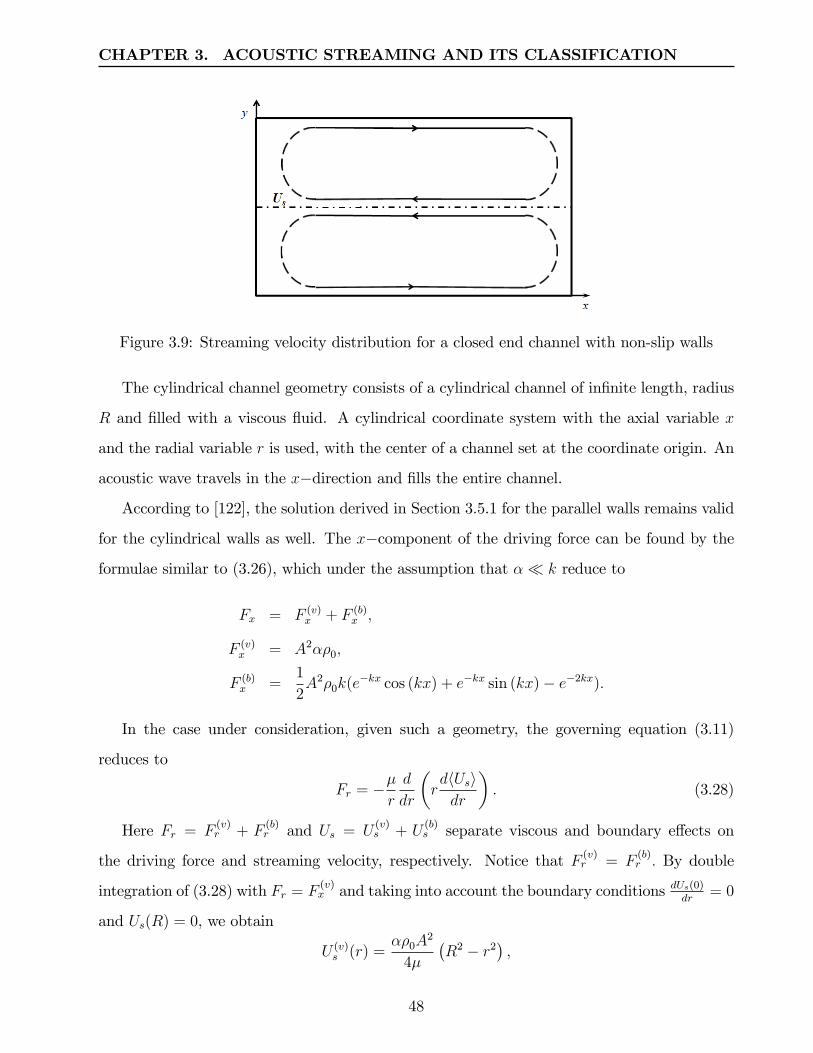
CHAPTER 3. ACOUSTIC STREAMING AND ITS CLASSIFICATION
Figure 3.9: Streaming velocity distribution for a closed end channel with non-slip walls
The cylindrical channel geometry consists of a cylindrical channel of infinite length, radius
R and filled with a viscous fluid. A cylindrical coordinate system with the axial variable x
and the radial variable r is used, with the center of a channel set at the coordinate origin. An
acoustic wave travels in the x−direction and fills the entire channel.
According to [122], the solution derived in Section 3.5.1 for the parallel walls remains valid
for the cylindrical walls as well. The x−component of the driving force can be found by the
formulae similar to (3.26), which under the assumption that α k reduce to
Fx = F (v)x + F (b)
x ,
F (v)x = A2αρ0,
F (b)x =
1
2A2ρ0k(e−kx cos (kx) + e−kx sin (kx)− e−2kx).
In the case under consideration, given such a geometry, the governing equation (3.11)
reduces to
Fr = −µr
d
dr
(rd〈Us〉dr
). (3.28)
Here Fr = F(v)r + F
(b)r and Us = U
(v)s + U
(b)s separate viscous and boundary effects on
the driving force and streaming velocity, respectively. Notice that F (v)r = F
(b)r . By double
integration of (3.28) with Fr = F(v)x and taking into account the boundary conditions dUs(0)
dr= 0
and Us(R) = 0, we obtain
U (v)s (r) =
αρ0A2
4µ
(R2 − r2
),
48

CHAPTER 3. ACOUSTIC STREAMING AND ITS CLASSIFICATION
which gives the streaming velocity profile resulting from viscous affects.
For the boundary steaming velocity U (b)s the authors used the numerical integration of
the differential equation obtained from (3.26) with Fr = F(v)z accompanied by the coordinate
substitution z = R− r.
The validity of this model is established by comparing it with a model for streaming between
parallel plates of infinite extent. The first difference noted between Nyborg’s solution for
parallel plates and cylindrical solution is that Nyborg’s solution is twice the magnitude of
the cylindrical solution for large-scale channels (e.g., R = 0.01 m). This happens because the
viscous force acting on a cross section within the cylindrical field is twice that acting on a
cross section between parallel plates [37]. For small-scale channels (e.g., R = 10−4 m) the two
solutions differ only slightly.
It is noted that, when channel diameters become very small the boundary layer induced
streaming dominates the flow. Therefore, it is important to obtain an accurate representation
of boundary layer streaming, and in particular to use a solution based on cylindrical coordi-
nates. While the main conclusions are proved to be in good agreement with Nyborg’s solution,
the use of Nyborg’s parallel plate theory will be incorrect for larger scale channels and the spe-
cific behavior in the acoustic boundary layer will be significantly different from that predicted
by parallel plate theory.
3.6 Applications of Acoustic Streaming
Acoustic steaming may be effective in accelerating certain kinds of rate processes and has
applications in localised micro-mixing, acoustic compressors, micro-fluidic devices, acoustic
levitation, ultrasonic medical diagnostic devices and ultrasonic cleaning of contaminant sur-
faces. Acoustic steaming has also attracted a lot of attention because it enhances heat transfer.
Recent interest in MEMS devices and especially in micro-fluidic devices involves a consid-
erable amount of research on the behavior of fluids in very small scale devices. In particular,
a focus has been on the impact of boundary layer induced streaming in micro-channels.
Thermal-acoustic interactions are found in many natural phenomena and industrial appli-
cations, such as pulse tube refrigerators, thermoacoustic refrigerators and engines. All of these
49

CHAPTER 3. ACOUSTIC STREAMING AND ITS CLASSIFICATION
applications involve mechanically driven acoustic fields in chambers with various media.
Acoustic steaming produced by sound wave near an interface boundary is characterized by
a relatively high-velocity gradient in the boundary layer. It is understandable that variety of
physical or chemical changes may be activated near such surfaces.
3.6.1 Cleaning
Acoustic streaming is viewed as the main technology in the non-contact cleaning of solid objects
from loosely adhering surface layers. If such an object is placed into a bath in which a sound
field exists, large acoustic streaming velocity gradients occur in the boundary layer, causing
high viscous stresses. These stresses are suffi cient to overcome the particle-to-object adhesion
forces and can aid in the removal of surface contaminants. The acoustic streaming velocity
increases with increasing frequency and power and with decreasing kinematic viscosity. The
acoustic boundary layer is very small compared to a typical hydrodynamic boundary layer at
the same velocity. This exposes small particles on the surface to much larger velocities and
increases the particle removal effi ciency.
Apart from AS, there is another effect, namely cavitation, that is observed in the sound
fields in a liquid medium. Cavitation is formation and collapse of bubbles that creates highly
localised streaming, or microstreaming, and finds its use in the cleaning processes. Nyborg
[121] was the first to analyze the microstreaming in the vicinity of the liquid-solid interface with
the presence of bubbles and small particles of comparable sizes. Microscopic contaminants are
best removed by lower frequency ultrasound in the range of 16—70 kHz, while submicroscopic
contaminants are often best removed by ultrasound at higher frequencies, on the order 400—
1000 kHz. Nyborg [122] describes the cleaning of vibrating membranes from viscous coatings
of paint or thin metallic coatings and observes that the removal of the coatings dominantly
happens in the areas of high streaming speeds.
However, as late as 1999, the physics of megasonic particle removal remained “largely
unexplained”, as stated in [59]. The theoretical and experimental investigations of the roles
that AS and cavitation play in cleaning process has been a subject of considerable interest. It
has been demonstrated that cavitation provides energy to detach undesired particles from the
50

CHAPTER 3. ACOUSTIC STREAMING AND ITS CLASSIFICATION
surface, while AS accelerates transport of the detached particles away from the surface. The
works by Deymeir and his colleagues [40, 41, 42, 83] have played crucial role in understanding
of AS and cavitation for the purpose of cleaning. A challenging aspect of using megasonic
agitation for cleaning purposes is to determine a regime that successfully removes the unwanted
particles without damaging the main substrate.
In modern microelectronics, the key issue is reducing the size of the devices. Applications
of AS to the removal of ionic contamination layers from silicon wafers are analysed, numerically
modelled and experimentally verified in [97]. In [21] Busnaina et al. present the experimental
results that show the effects of power, temperature and time on the removal effi ciency of silica
particles from silicon wafers. The experiments described in [22] demonstrate advantages of
megasonic non-contact cleaning and polishing of wafers, compared to contact techniques, such
as brush cleaning.
Brereton and Bruno [18] describe the experimental investigation of micron particle removal
by focused ultrasound. Their results are combined with analytical and numerical modelling.
The experimental results indicate that successful removal of particles depends not only on fre-
quency and amplitude of acoustic excitation but also on acoustic energy density and exposure
time.
The experimental research of Lamminen et al. [88] shows that ceramic membranes can be
effectively cleaned using ultrasound without damage to the membranes. The authors notice
that AS alone in their experiments did not have significant effect on cleaning.
3.6.2 Enhancement of transport
It is well known that the presence of AS increases the chemical reaction rate over a surface.
First, it can be connected with the removal action of streaming, when inhibitory layers are
removed and they don’t accumulate on near reaction surfaces and don’t slow down the devel-
opment processes. On the other hand, the action can be associated with enhanced convection
of reactant spices when AS provides more even transport of spices across the electrode and de-
creases the depletion of those. The use of AS in electrochemistry suggests significant benefits:
decrease the process time and increase the deposition rate.
51
CHAPTER 3. ACOUSTIC STREAMING AND ITS CLASSIFICATION
Analytical and numerical models by Nilson and Griffi ths [115] and Nilson et al. [116]
address LIGA development, which includes the removal of the exposed material by chemical
dissolution in a development bath. They demonstrate that the enhancement of LIGA devel-
opment rates results from AS flow that circulates most of the fluid within HAR vias, thereby
significantly increasing ion transport.
There are a number of occasions within industry where substances need to be permeated
through a porous material, for example, dying leather or adding flavours to food. One of the
methods that helps to enhance significantly the diffusion process in these industrial applications
is AS. Haydock and Yeomans [69] describe the effects of Eckart streaming on diffusion into
a porous material. According to their simulations the force inducing AS acts throughout the
material which leads to a higher internal flow rate and to higher rate of diffusion. The authors
find that streaming can enhance diffusion by a factor of up to 10.
3.6.3 Enhancement of heat transfer
Westervelt [174] studies the increase in heat transfer due to AS and concludes that the effect
of sound waves on heat transfer is dominantly a result of modification of the convective flow
in the inner boundary layer. According to Westervelt, especially effective heat transfer occurs
when the vibration amplitude exceeds the boundary layer thickness δ by a significant ratio
and Reynolds number for streaming velocity is the critical parameter which determines the
increase of heat transfer rate.
Vainshtein et al. [164] analyse heat transfer between the parallel plates in the presence of
Rayleigh streaming. In their experiments, the two plates are kept at different temperatures.
Their analysis shows that the heat transfer could be enhanced by approximately one order of
magnitude if a high-amplitude, high-frequency sound field is used.
Huyn et al. [72] and Loh et al. [100] investigate experimentally and numerically the
momentum and heat transfer due to AS induced by ultrasonic vibrations and observe a sub-
stantial decrease in the hot plate temperature. Lee et al. [91] consider the streaming outside
the boundary layer, which is relevant to heat and mass transfer.
Lei et al. [94] investigate numerically the natural convection in differentially heated rec-
52

CHAPTER 3. ACOUSTIC STREAMING AND ITS CLASSIFICATION
tangular enclosure under various acoustic fields. Their work is connected to the technologies
of materials processing such as semiconductors, GaAs, In-Sb, etc. by directional solidification
from their melt.
Parker and Welsh [126] and Copper et al. [29] investigate experimentally the effect of a
sound field on a heat transfer from the horizontal flat plates. Engelbrecht and Pretorius [47]
carry out the experimental study on the influence of the sound field on the transition from
laminar to turbulent flow in the boundary layer associated with natural convection from a
vertical flat plane.
One of the examples of using AS properties is the cooling of electronic devices. The size of
the conventional motor-driven fans that are normally used to provide an effective heat transfer
cannot come up with the process of the constant miniaturization of the electronic components.
Acoustic streaming offers an alternative way to extent heat transfer. As Boluriaan and Morris
mention [15], in the case of standing waves, AS carries heat from a hot surface to a cold
surface. In the case of traveling waves, it carries heat away. These authors also emphasize
that enhancement in heat transfer achieved by AS becomes particularly important when other
means of heat transfer enhancement are diffi cult to apply. For example, in a microgravity
environment relevant to aerospace applications, natural convection is eliminated. In this case,
a sound field can be used to generate AS and provide the required heat transfer.
Acoustic streaming offers some obvious advantages for applications in the cooling of elec-
tronic devices. As Lasance and Aarts point out [90], the following improvements are expected
when comparing AS with fans: a much lower noise level, better thermodynamic effi ciency,
intrinsic higher reliability, miniaturisation easier than with fans.
In some practical situations, solid-liquid phase change occurs, e.g., melting or solidification.
For example, this happens in casting and welding, crystal growth, melting of edible oil. Oh et
al. [123] experimentally compare two types of melting process: natural melting and melting
with ultrasonic vibrations. The acceleration of the melting process the authors attribute to
ultrasonic effects including AS.
53

CHAPTER 3. ACOUSTIC STREAMING AND ITS CLASSIFICATION
3.6.4 Applications to biology and medicine
Many theoretical and experimental studies have been done on the possible bioeffects due to
AS in diagnostic or therapy ultrasound applications, especially when applied to humans.
As pointed out by Starritt et al. [152], streaming may be set up in any path of a reasonable
length in the biological fluids such as blood, urine within bladder, etc. These authors inves-
tigate the enhancement of streaming in high amplitude diagnostic pulses in water. Zauhar et
al. [178] extended the previous results by investigating AS in biological fluids, for which the
absorption is significantly higher than for water.
Most diagnostic systems use focused and finite-amplitude pulsed ultrasound. Wu and Du
[175] develop a theoretical model that allows them to calculate the streaming velocity along
the beam axis generated by a continuous acoustic wave. The results of calculations are useful
in clinical ultrasound applications.
Nightingale et al. [114] report the results of clinical studies in which AS was successfully
used to differentiate fluid-field leasions (cysts) from solid leasions in the breast. They take
into account the fact that AS cannot be induced in a solid lesions and its presence indicates a
cyst. Jonsson et al. [75] describe their experiments which help to distinguish between various
stages of a sinus infection. In their studies they confirm the hypothesis that AS is not induced
at clinically acceptable intensity levels in infectious fluid because of its high viscosity, but
detected AS means a strong indication that the sinus content is noninfectious fluid.
It has been observed in early experiments that an ultrasonic field will produce vortex and
other movements in biological cells. If cells are not free to move but fixed, they may experience
shear viscous forces due to nearby streaming fluid flow. Sonic techniques are widely used in
biochemistry for disrupting cells. Sakharov et al. [146] show that high-frequency ultrasound
accelerate clot reduction. One of the mechanisms of this effect is the enhancement of mass
transport by AS, i.e., ultrasound-induced macroscopic flow or stirring around the clot. Devcic-
Kuhar et al. [39] in their in vitro study examine and compare the effects of standing and
traveling acoustic waves on enhancement of thrombolysis. The authors conclude that the
enhancement of clot dissolution is much more essential in traveling than in standing acoustic
waves. Acoustic streaming and accompanying shear stress are the main effects of ultrasound
54

CHAPTER 3. ACOUSTIC STREAMING AND ITS CLASSIFICATION
that dominantly appear in traveling acoustic fields, but they are negligible in standing acoustic
fields.
In their review Vaezy et al. [163] show that high intensity focused ultrasound (HIFU) is
very effective method of hemostasis for blood vessels and for solid organs. Acoustic streaming,
as one of the effects of ultrasound, is the most important and practical since it helps to push
away the blood from a bleeding site, either back into a bleeding vessel, or just out of the way.
This action provides two advantages: the pool of blood does not obstruct the view during
surgery and the absence of blood allows a better deposition of the thermal energy of HIFU
and thus an enhanced hemostasis.
In their resent study, Ehlers and Koiller [48] show that AS produced by nanoscale membrane
vibrations can be widely used in cell biology. According to their calculations, a traveling surface
acoustic wave produces a non-negligible boundary layer surrounding the cell. Therefore, AS
leads to the enhancing of localised diffusion processes and chemical reactions.
3.6.5 Micro-mixing of Materials
Detailed regulation on transport of fluids as well as of various immersed objects as large
molecules and whole cells is very useful for obtaining materials with the fine structures and new
functions. The advantage of utilizing AS is that a specific part of the material can be selectively
stirred without any mechanical stirrer. This allows to control the mixing of the samples
from outside of the cell. Murata et al. [110] describe the use of acoustic mixing to polymer
processing in order to improve the quality of molded objects. By mixing polymeric materials
in the mold, the number of defective objects can be reduced because the degree of orientation
in the materials is lowered. Suri et al. [157] study experimentally the possibility of developing
a mixer based on the transport properties of AS. The advantage is clearly demonstrated: it is
possible to spin a water solution inside a closed bottle without any mechanical contact, even
if streaming is generated outside the bottle. The most influential parameters affecting the
mixing effi ciency are a position of the container in the acoustic field and the wave amplitude,
while the frequency and the size of the transducers have a little effect.
55

CHAPTER 3. ACOUSTIC STREAMING AND ITS CLASSIFICATION
3.6.6 Levitation Effects
Noncontact manipulation of particles, droplets and bubbles using energy of acoustic waves as
the levitation force is an active area of investigation. It is possible to use near-boundary AS to
levitate these various objects, i.e., to provide noncontact transport of different planar objects.
Nomura et al. [117] show how traveling waves can be used for noncontact transport technology
and report studies related to streaming velocity as a function of water height.
The drying of droplets of liquid mixtures and solids solutions is of significant interest in
many industrial applications, for example, where the liquid vapor is a fuel for combustion
process or when powders are produced by spray drying process. Yarin et al. [177] investi-
gate experimentally and theoretically the evaporation of solution droplets levitated in strong
acoustic fields. The authors show that droplets of liquids in acoustic levitators evaporate
mostly due to the convective effect of AS arising near the free droplet surface.
56

Chapter 4
Tools for Numerical Modelling
In this chapter, we briefly describe the software tools used in the thesis for the purpose of
numerical modelling: PHYSICA, PHOENICS and COMSOL. Additionally, we present the
main features of VisualDOC, a software system for design optimisation.
4.1 General Principles of Numerical Modelling
Physical processes are normally described by mathematical equations with partial derivatives
that are applied to a specific geometric domain and are subject to the initial and/or boundary
conditions. Such equations do not normally admit analytical solutions in close forms, except
for very simple cases, and have to be solved approximately by various numerical techniques.
The area of developing numerical methods, their software implementation and application
is known as Computational Modelling. The application areas that are handled by means of
computational modelling include but not are limited to
• Computational Fluid Dynamics (CFD), that handles fluid flow, heat transfer, combus-
tion, solidification and other related phenomena;
• Computational Solid Mechanics (CSM ), that studies deformation, dynamics, stress and
failures in solid structures;
• Computational Electromagnetics (CEM ), used to solve the problems that arise in elec-
tromagnetics, electrostatics and magneto-statics.
57

CHAPTER 4. TOOLS FOR NUMERICAL MODELLING
The requirements of modern manufacturing calls for the development ofmulti-physics or co-
disciplinary numerical tools that are capable to capture possible interactions between various
physical phenomena (e.g., fluid, thermal, mechanical and electrical).
In this thesis, we study the phenomena of electrodeposition, acoustics, fluid flow and their
interactions. For our purpose, the most suitable equation is the so-called general transport
equation. It can be written for a dependent variable ψ in the form
∂(ρψ)
∂t︸ ︷︷ ︸transient term
+ ∇ · (ρUψ)︸ ︷︷ ︸convection term
= ∇ · (Γ∇ψ)︸ ︷︷ ︸diffusion term
+ Sψ︸︷︷︸source term
. (4.1)
Its four terms are called due to the main area of its application, the CFD. Here t is time,
and under the CFD interpretation, U is understood as a velocity, while Γ is the diffusion
coeffi cient. As far as the variable ψ is concerned, we may set
• ψ = 1 for the continuity equation;
• ψ = C for concentration equation;
• ψ = U for the momentum equation.
Notice that many physical processes that are studied in fluid mechanics are described by a
pair of equations, one of which is (4.1) and the other is
∂ρ
∂t+∇ · (ρU ) = 0, (4.2)
which is known as the continuity equation and is derived from (4.1) if ψ = 1.
To solve an equation similar to (4.1) numerically, the domain is split into fairly small
non-overlaping fragments, and for each fragment the derivatives are replaced by their discrete
analogues. This reduces the original problem described by partial differential equations to a
system of algebraic equations. Such a process is known as discretisation.
The process of splitting the domain into the fragments (cells) is known as meshing. Tradi-
tionally, there is a distinction between structured meshes and unstructured meshes. A struc-
tured mesh possesses regular connectivity. The cells of a structured mesh are either quadrilat-
erals in 2D and information on their connectivity can be stored in a 2D array (matrix), or the
58

CHAPTER 4. TOOLS FOR NUMERICAL MODELLING
cells are 3D hexahedra with the relevant information to be organised as a 3D array. Connec-
tivity of an unstructured mesh can be irregular. The storage requirement for an unstructured
mesh can be substantially larger than a matrix representation of a structured mesh, since for
each cell the information on its neighbours must be explicitly stored.
One of the simplest, yet effective forms of discretisation is the Finite Difference Method
(FDM), which replaces the derivatives (with respect to space and time) by the finite differences
computed at selected points (e.g., nodes of a mesh and time steps). FDM is restricted to simple
geometries and regular meshes. See [141] and [159].
A different approach to discretisation is implemented in the form of the Finite Element
Method (FEM ). This is a variation of a more general Galerkin method with the polynomial
approximation functions. Without going into technical details, here we only mention that the
FEM reduces partial differential equations either to systems of algebraic equations (for the
steady state problems) or to systems of ordinary differential equations (for transient prob-
lems). In the latter case, the obtained ordinary differential equations need further numerical
integration. See [12] and [127].
A mesh that is used in the Finite Volume Method (FVM ) creates polyhedral Control
Volumes (CV ). This method can be seen an advanced variation of the FDM. In this section,
we discuss the cell-centered modification of the FVM, as opposed to the cell-vertex variant.
The centre of each CV is associated with the values of independent and dependent variables
computed as the average value across the whole CV. FVM is currently the most popular
method in numerical modelling. See [127] and [166].
Below we illustrate the principles of discretisation used in the FVM. A good comparison
of discretisation in the FVM and FEM is presented in [49].
The goal is to reduce the pair of equations (4.1) and (4.2) to a set of linear algebraic
equations, which can then be solved to obtain the value of the dependent variable at each CV
centre. Discretisation starts with numerical integration of an equation over a control volume,
followed by appropriate approximations for fluxes across the boundary of each CV.
We explain how this approach works for each of the four terms in (4.1), without presenting
all technical details. In the case of the convection and the diffusion terms, the volume integral
59

CHAPTER 4. TOOLS FOR NUMERICAL MODELLING
is expressed in terms of the area integrals over the surface of the CV in accordance with Di-
vergence theorem, also known as the Gauss-Ostrogradsky theorem. Recall that the Divergence
theorem states that the outward flux of a continuously differentiable vector field F through a
closed surface S is equal to the volume integral of the divergence of the region V inside the
surface. Formally, it can be written as∫∫∫V
(∇ · F )dV =
∫∫S
(F · n) dS, (4.3)
and can be understood as a conservation law which states that the total volume of all sinks
and sources (the left-hand side), is equal to the net flow across the volume’s boundary (the
right-hand side). For each variable in our descretised terms, we use the subscript “P”to refer
to its updated value in a point P , and additionally the superscript “0” for the previously
available value.
• For the transient term we discretise the time derivative to achieve∫V
∂(ρψ)
∂tdV ≈
(ρPψPVP − ρ0
Pψ0PV
0P
)∆t
.
• For the convection term, we use (4.3) with F = U to deduce∫V
∇ · (ρUψ)dV =
∫S
ρψ (U · n) dS ≈∑f
ρf (U · n)f ψfAf ,
where∑
f denotes the summation over the faces of a CV, Af is the area of each face and
n is the normal vector pointing out of the CV’s face. For each face, the face density ρf
and ψf can be appropriately found [127].
• For the diffusion term, a similar approach will result in∫V
∇ · (Γ∇ψ)dV =
∫S
Γ (∇ψ · n) dS ≈∑f
Γf (∇ψ · n)f Af ,
where again the summation is taken over all faces of a CV, and the diffusion coeffi cient
Γf is appropriately estimated [127].
• Finally, for the source term, ∫V
SψdV ≈ SψVP.
60

CHAPTER 4. TOOLS FOR NUMERICAL MODELLING
If Sψ depends on ψ, then this dependence can be included to increase stability. Usually,
in this case the source term is linearised as Sψ = SC − SPψP , so that∫V
SψdV ≈ VP (SC − SPψP ). (4.4)
The descretisation scheme for the transient and the convection terms can be used to de-
scretise equation (4.2).
As a result, we obtain a system of linear algebraic equations for finding the value of ψ in
the next iteration.
These and similar principles are implemented in various pieces of numerical modelling
software, including those discussed in the remainder of this chapter.
4.2 Multi-Physics Package PHYSICA
In this work, we mainly use the package PHYSICA, which is a modular suite of software
components for the simulation of coupled physical phenomena in 3D and time. PHYSICA
was developed at the University of Greenwich, U.K. in 1990s and is distributed by Physica
Ltd, Oxon, U.K. See [35, 36, 129].
In release 2.10, PHYSICA contains modules to solve problems by running steady-state or
transient simulations. PHYSICA is programmed in Fortran 77 and is based on finite volume
techniques on 3D structured and unstructured meshes.
The package can be linked with a pre-processor such as FEMGV [53]. At the pre-processing
stage the following actions are taken:
• define the geometry;
• generate the mesh of the domain;
• define boundary patches and apply boundary conditions;
• define material and physical properties of the elements.
In the solving stage, a variety of modules and interacting routines available within PHYS-
ICA are engaged, e.g., Fluid Flow, Heat Transfer, Scalar Variable, Solidification, Turbulence,
61

CHAPTER 4. TOOLS FOR NUMERICAL MODELLING
Free Surface, Visco-Elastic etc. The relevant mathematical equations, such as (4.1) and (4.2)
are discretised and solved using finite volume techniques and the input specifications. In
PHYSICA the numerical modelling of multi-physics phenomena engages all relevant software
components into a single numerical scheme.
PHYSICA is an open framework that allows the users to write and implement their own
code. For an experienced user this provides the required level of flexibility. To run a problem
PHYSICA an INFORM text file should be prepared. In this file all modules which solve
the problems under consideration are defined and the initial/boundary conditions, material
properties etc. are specified.
At the post-processing stage PHYSICA can be linked with post-processing software pack-
ages such as FEMGV or TECPLOT [158] for visualisation of the results. The resulting data
may be presented in the form of vector plots, contour plots, animations, etc.
In this thesis, we use PHYSICA to implement our approach to modelling of electrodepo-
sition based on the Explicit Interface Tracking Method. The flexibility of PHYSICA allows
us to use it for handling the numerical models of enhanced electrodeposition.
4.3 CFD Software Package PHOENICS
PHOENICS is the principal product of an engineering-software company CHAM (Concentra-
tion Heat and Momentum Ltd), located in Wimbledon, England; see http://www.cham.co.uk.
The name is an abbreviation of Parabolic, HyperbolicOr E llipticNumerical IntegrationCode
Series. The first version of PHOENICS was launched in 1981, and since then it remains one
of the most popular software packages in the area of CFD. There is chain of international
conferences of PHOENICS users and a specialized The PHOENICS Journal, run since 1988.
UnlikePHYSICA which is essentially a solver, thePHOENICS code is fully self-contained,
i.e., it provides a tool for creating a geometry of objects, grid generation of the computational
domain, solution of the relevant equations, and post processing done in a 3-D virtual real-
ity interface. It is written in Fortran, and has a flexible interface for introducing arbitrary
equations. See the reference manual [128].
PHOENICS is a finite volume CFD package. The computational domain is covered by
62

CHAPTER 4. TOOLS FOR NUMERICAL MODELLING
control volumes of finite size (cells). The mesh is structured, but it need not to be uniformly
spaced. The cells are “topologically Cartesian”, i.e., in the 2D case a cell is a quadrilateral,
while in the general 3D case a cell is a polyhedron with six sides and eight corners. The
finite-volume equations are derived by integration of the differential equations over a cell.
Scalar values, such as pressure, are stored at the cell centre and are assumed to be repre-
sentative of the whole cell. By contrast, vector quantities, such as velocity, are generally stored
at the cell faces and define the value of the variable over the area of the face only.
The method of storing scalars at the cell centre and vectors at the cell faces is known as
the staggered grid arrangement. The reason for introducing the staggered grid arrangement
for velocity components is to suppress pressure oscillations known as checkerboard effects; see
[127]. If the checkerboard pressure distributions are not suppressed, the resulting velocity
fields will appear physically unrealistic.
In the staggered grid, the pressure gradient terms will act at the face of the CV and
therefore will give the driving force for velocity where it is required, at the velocity storage
points. Another benefit of this grid arrangement is that it will be no need to interpolate the
value of velocity components at the main grid cell faces for the calculation of fluxes, since there
are already available.
However one serious drawback of the staggered grid arrangement is that it cannot be
easily extended to unstructured meshes. An alternative is provided by the Rhie and Chow
algorithm [140], which approximates mass fluxes at cell faces. This has proved invaluable in
the development of unstructured codes and is used, e.g., in PHYSICA.
In this thesis, the use of PHOENICS is limited to the numerical modelling of flow phe-
nomena in a plating cell; see Chapter 6.
4.4 Multi-Physics Package COMSOL
COMSOL Multiphysics [28] is a software product by COMSOL Group. The company
was founded in 1986 in Stockholm, Sweden, and launched the first version of COMSOL
Multiphysics in 1988; see http://www.comsol.com. The package is capable of numerical
modelling of various physics phenomena and of combining multiple physical effects. More
63

CHAPTER 4. TOOLS FOR NUMERICAL MODELLING
than 100,000 users perform their numerical modelling by COMSOL Multiphysics. The
conferences of users are held regularly; only in 2011 three such conferences took place in
different parts of the world.
Unlike PHYSICA or PHOENICS that use the Finite Volume method, COMSOL Multi-
physics is based on a Finite Element Modelling platform. It is linked with many established
pieces of software, such as MATLAB, Inventor and Pro/Engineer.
Similarly to PHOENICS, all steps in the modelling process are facilitated by COMSOL
Multiphysics: defining a geometry, meshing, specifying the physics, solving and then visu-
alizing the results.
The built-in drawing tool or files from a CAD package can be used to create geometries.
The computational domain is covered by an unstructured mesh of tetrahedral cells.
Recall that one of the flexible features of PHYSICA allows users to write and include their
own simulation code. The COMSOL Multiphysics user interface offers an alternative by
giving the option to specify user-own partial or ordinary differential equations and link them
with other physics interfaces.
COMSOL Multiphysics has a modular structure, with modules responsible for solving
various physical problems. Most recent advanced versions include, among others, the following
modules: CFD, Heat Transfer, Acoustic, Chemical Reaction Engineering, Electrodeposition,
MEMS, Structural Mechanics, Microfluidics, Particle Tracing etc. The programing tool for
parametric analysis and optimization is provided.
In general, the modules are mutually compatible. In COMSOL Multiphysics the use
of the modules is sequential, e.g., a solution by the CFD module becomes the input for, e.g.,
the Heat Transfer Module and further on. This is achieved by specialised coupling variables.
Recall that in PHYSICA, all relevant modules are made active simultaneously, in a single
numerical scheme.
In this thesis, we use COMSOL Multiphysics for solving the CFD problems. We also
rely on the Acoustic module, which, however, allows the user to observe only the first order os-
cillations and not the second order phenomena, such as acoustic streaming; see Chapter 7. The
most recent version of COMSOL Multiphysics 4.2a includes the Electrodeposition module
64

CHAPTER 4. TOOLS FOR NUMERICAL MODELLING
Software Area Discretisation Method Mesh Self-ContainedPHYSICA Multi-physics Finite Volume Structured/ No
UnstructuredPHOENICS CFD Finite Volume Structured YesCOMSOL Multi-physics Finite Element Unstructured Yes
Table 4.1: Comparative characteristics of modelling software
which we use in Sections 5.4 and 5.5 to validate our approach to the numerical modelling of
electrodeposition. Still, the structure of the COMSOL module prevents us from using it for
modelling electrodeposition enhanced by the forced flow or acoustic streaming; see Section 5.3
for a discussion.
The properties of the software packages discussed in this chapter are summarised in Ta-
ble 4.1.
4.5 Design Optimisation Software VisualDOC
VisualDOC is a software product by Vanderplaats Research & Development (VR&D), Inc.;
see \\http:www.vrand.com. The company was founded in 1984 by G.N. Vanderplaats and is
based in Colorado Springs, USA. The company’s main product is an optimiser package DOT
(Design Optimization Tools) that is capable of solving nonlinear constrained or unconstrained
optimization problems. VisualDOC is another popular product, launched in 1998, which
allows the user to add optimisation to various design tasks. VisualDOC (Visual Design
Optimisation Control) is a general purpose optimisation tool with modules for numerical non-
linear optimisation and statistical analysis.
VisualDOC includes modules that are capable of handling the problems of:
• Design of Experiments (DoE);
• Gradient and Non-gradient optimisation;
• Response surface optimisation;
• Probabilistic and Robust optimisation.
65

CHAPTER 4. TOOLS FOR NUMERICAL MODELLING
The components of VisualDOC are the database, the design modules, the Graphical
User Interface (GUI), post-processing visualization tools and the response program interface.
Design modules encapsulate the optimisation, approximation and statistical algorithms.
In the preliminary stage of design of a system or process, the developer starts with a
definition of the design project, formulates all aspects of the design, sets major objectives of
the project and identifies the design parameters that can be controlled. The resulting design
project specification can be entered in VisualDOC in terms of definitions of the design
variables, the objective function(s) and constraints. The resulting problem can be solved by a
particular optimisation module from the VisualDOC optimisation library. The optimisation
results can be used for post-processing activities.
The purpose of running experiments is to characterise unknown relations and dependencies
that exist in the process under consideration. Based on a rather small number of observations,
the user wants to deduce how the process is influenced by a set of chosen design variables and
how it will respond to variations in the values of those variables. VisualDOC allows the user
to establish variable-objective relationships, to identify most influential design parameters and
its optimal numerical values.
VisualDOC has a functional module to perform the DoE analysis. The DoE can be used
either as a separate program for statistical analysis of the design or as a tool to perform DoE-
based Response Surface (RS) optimisation . The latter approach is effective for relatively small
number of design variables and is based on polynomial approximation.
Let us illustrate how VisualDOC can be used to analyse numerical experiments on basic
electrodeposition; see Section 5.7 for a detailed discussion. Recall that the quality of an ED
process in small vias is characterised by various metrics, see Section 2.5.2. It is important
to know how the filling metrics and the completion time are influenced by various regime
parameters of ED. Let X1, X2, . . . , Xn be the design variables. Ideally, we would want to know
the response of the process to any particular set of values of the design variables. However,
due to the complexity of the process such a link is hard to establish explicitly, in a form a
function y = F (X1, X2, . . . , Xn). The DoE technique allows us to find a good approximation
f(X1, X2, . . . , Xn) of an unknown function F in form of the RS. Suppose we fix q arrays of
66

CHAPTER 4. TOOLS FOR NUMERICAL MODELLING
values of the design variables, so that the values in the i−th array are X(i)1 , X
(i)2 , ..., X
(i)n ,
where i = 1, 2, · · · , q. For each set of values X(i)1 , X
(i)2 , ..., X
(i)n , the process respond Yi can be
found. Based on these values, VisualDOC will find the RS as a polynomial approximation
f(X1, X2, . . . , Xn) of the desired function F . Once the RS formula, as a polynomial function
of the design variables is obtained, the user can perform various post-processing tasks:
• to identify the most influential parameter;
• to determine the optimal numerical values of the design variables that deliver the required
response;
• to predict the response for a given range of values of the design variables.
67

Chapter 5
Numerical Modelling of BasicElectrodeposition
In this chapter, we describe our approach to numerical modelling of basic electrodeposition.
A concise literature review of the relevant issues is presented. The main assumptions are
stated. The governing equations are presented and their discretisation is discussed. We review
suitable software tools and justify the chosen piece of software. A novel explicit interface
tracking technique is presented, that monitors the interface between the electrolyte and the
deposited metal over time. For this method, we report the validation results and perform
a parametric study. See Table 1 for notation. The material of this chapter corresponds to
Objectives 1, 2 and 3 of the thesis set in Section 1.1. The results related to this chapter are
published in [71, 153, 154, 155].
5.1 Literature Review
In this section, we overview known approaches to numerical modelling of electrodeposition.
The complexity of electrodeposition as a multi-physics process does not allow us to obtain the
analytical solutions even for fairly simple models. Therefore, research on modelling of ED is
mainly aimed at obtaining numerical solutions with an aid of a software package.
In this section we focus on several issues related to numerical modelling:
• mathematical modelling, i.e., the use of equations that govern the process if they differ
from the classical ones, discussed in Chapter 2;
• approaches to numerical solutions of the governing equations;
68

CHAPTER 5. NUMERICAL MODELLING OF BASIC ED
• software tools used for numerical modelling.
Recall that, as mentioned in Section 2.5, a possible way of improving the quality of elec-
trodeposition is to affect its kinetics by various additives. A large part of the publications
reviewed in this section is devoted to modelling of ED in the presence of additives. These pub-
lications are less relevant to this thesis but contain useful modelling ideas. As in Chapter 4, we
use abbreviations FDM, FEM and FVM for the Finite Difference, Finite Element and Finite
Volume methods, respectively.
As follows from the consideration in Section 2.4, the knowledge of the current distribution
is essential for ED modelling. Georgiadou [62] develops a numerical method for determining
the current density distribution in the parallel-plate electrochemical reactors with multi-ion
electrolytes, assuming steady-state, 2D rectangular geometry and constant properties. The
model is based on the transport partial differential equation that consists of linear terms
of diffusion and laminar convection, as well as of nonlinear terms of ionic migration. The
boundary conditions include flux conditions and nonlinear terms associated with exponential
kinetics of electrode reaction in the Butler-Volmer form. The diffusion and migration terms in
the governing equation are discretised by means of the centered analogue of the FDM. On the
other hand, the convective term is discretised using an upwind differencing scheme. To specify
the flux boundary conditions the method of “false boundaries”is employed. In this method,
a fictitious point outside the domain and corresponding value of the unknown variable are
introduced for a purpose of derivative approximation. A nonuniform rectangular mesh of fine
size near the electrode surface is used. The method is effective at high velocities; however, it
is only valid for rather simple geometries.
To determine the current density and concentration distribution along the cathode,
Boovaragavan and Basha [16] develop a semi-analytical method with a minimum number
of iterative procedures and assumptions regarding the simplified tertiary current distribution.
The assumptions include: (i) only a cathodic reaction is considered; (ii) the overpotential of
the anode is zero; (iii) the transport and kinetic parameters do not vary in space and time,
and (iv) the physical properties of the electrolyte are constant.
69

CHAPTER 5. NUMERICAL MODELLING OF BASIC ED
The authors attempt to solve the steady-state laminar convective diffusion equation
V (∇C) = D ∇2C (5.1)
for ionic concentration together with the Laplace equation ∇2φ = 0 for the electrical potential.
The analytical solution of equation (5.1) is obtained using the Laplace transformation. As a
result, the surface concentration and the local current density are found. Then the surface
concentration is represented as a power series, with the coeffi cients computed by a simplified
Butler-Volmer equation. The technique is reported to work well for finding current distribu-
tions, provided that either electrolyte flows between parallel electrodes or the electrodes move
in a stationary electrolyte. The method is computationally effi cient, since it iterates for only
one variable (concentration). It can be further extended to handle irregular geometry, unusual
boundary conditions or multi-ion electrodeposition. However, the semi-analytical method com-
putes simplified tertiary current density and surface concentration distribution, ignoring the
migration contribution, and this makes it hardly applicable to modelling of ED in trenches and
through vias. For these vias, the migration term in the transport equation cannot be neglected
and, due its strong non-linearity, only a numerical method is possible.
The principal diffi culty of modelling of ED is the need for monitoring the position of the
deposited layer, which leads to models with variable geometry. Such models allow us to track
the position of the interface between the electrolyte and the deposited metal.
Georgiadou et al. [61] present a quasi-steady-state numerical model for copper ED in
trenches. The model takes the highly nonlinear boundary conditions for multiple reactions;
laminar fluid flow, diffusion and migration; multiple species transient behavior; 2D and 3D
capability; moving boundaries for simulation of shape evolution during deposition. The current
of copper electrodeposition is expressed by Butler-Volmer equation. A single additive that
suppresses metal deposition is included, and its effect is expressed by an empirical function.
The primary objective of the paper is to develop numerical methods with moving boundary
capabilities for simulating evolution of the deposited layer. Two numerical methods are used
for the simulations: (i) a version of the FDM with curvilinear coordinates, and (ii) a FEM
based on a standard Galerkin discretisation scheme. In both methods, in each time step, the
70

CHAPTER 5. NUMERICAL MODELLING OF BASIC ED
following actions are taken:
• a solid boundary is moved along the local normal to the surface undergoing electrode-
position by a distance corresponding to the volume of the metal deposited according to
the local current density;
• the current density is obtained by computation of the boundary flux of copper ions;
• the geometry is remeshed after the boundary has been redefined by moving and redis-
tributing the boundary nodes in the previous time step.
This model demonstrates superconformal filling, however, no detailed comparison with
experimental data is provided and the model is not extended to handle multi-additives systems.
In computational mathematics, a popular technique to track moving interfaces in complex
situations is the Level Set Method (LSM) jointly developed in the 1980s by S.J. Osher and J.A.
Sethian [124]; see also subsequent books [125] and [148]. For handling models of electrodepo-
sition, the LSM is adapted in a three-part paper by Adalsteinsson and Sethian [3]-[5]; see also
[2].
The LSM is used to track implicitly the motion of the metal/electrolyte interface. The
LSM is highly robust, accurate and is applicable to rather complex motions. It can easily
handle sharp corners and topological changes, such as interface splitting and merging. In a
typical version of the LSM, a time-dependent Ψ level-set function is defined over the entire
region, which measures distance to the interface. In the ED applications, we define Ψ = 0 on
the interfaces, Ψ < 0 for the solid copper region and Ψ > 0 for the electrolyte domain. The
level-set equation describing the interface evolution is given by
∂Ψ
∂t+ v |∇Ψ| = 0, (5.2)
where v is the velocity of interface in its normal direction. In the LSM, v is defined not only on
the zero level set, but on all level sets throughout the computational domain. On the zero level
set, v is naturally defined by the deposition rate. For other parts of the region, the values of
v known as extended velocity, vExt, have to be computed. As suggested by Sethian [149], this
71

CHAPTER 5. NUMERICAL MODELLING OF BASIC ED
can be done by the Fast Marching Method (FMM). This method uses a temporary distance
function ΨTemp that matches Ψ at their zero level sets and finds vExt by solving the equation
∇ΨTemp · ∇vExt = 0,
where vExt matches v on the interface. As a result, the general level-set equation can be written
as∂Ψ
∂t+ vExt |∇Ψ| = 0.
Josell, Moffat, Wheeler and their co-authors [76, 78, 79, 108, 109, 172], as well as West
et al. [173] use the LSM for tracking the interface position in an ED process along with a
Curvature Enhanced Accelerator Coverage (CEAC) model. The CEAC technique involves
• enhancement of local metal deposition rate with increasing coverage of accelerating
species on the metal/electrolyte interface, and
• significant change of local coverage of catalyst in vias due to the decreasing of the interface
area, which is reduced during growth of the deposition level.
As a rule, in the quoted papers the equation for concentration does not contain the mi-
gration term. The source term describes the flux loss from the electrolyte at the interface.
The current distribution is defined by the Butler-Volmer equation, with the cathode reaction
alone taken into consideration. Dependence of this equation on accelerator coverage adsorbed
at the interface is determined experimentally. The finite difference equations are derived for a
nonuniform cell centered unstructured mesh using the finite volume method.
The authors assert that this combined method effectively predicts superconformal depo-
sition in trenches and vias for various metals (copper, silver, nickel and gold). On the other
hand, Sethian and Shan [150] with the references to [171] and [172] point out that the described
techniques may fail to accurately predict the experimental results, since the exact relations
between the deposition rate and the curvature of the interface are not clear enough.
Bouni and Petzold [19] present a novel methodology for solving governing equations of
electrochemistry under conditions of dilute electrolyte solution for systems with irregular and
72

CHAPTER 5. NUMERICAL MODELLING OF BASIC ED
moving boundaries. They use a version of the LSM to track the interface. In their numerical
solution, the authors split the governing equation for concentration into three terms, respon-
sible for reaction, diffusion and migration, respectively, and then numerically integrate the
chemical concentration fields corresponding to each set by the FVM. The resulting algorithm
is effi cient, scales well with grid refinement, and is easy to parallelise. This approach is further
extended in [20] to handle the 3D case. A new feature of the extended model is that it handles
electroneutrality of the solution in their formulation, which is usually neglected by others due
to the computational diffi culty it presents.
Among the models studied by Chivilichin, Landau, Malyshev and their co-authors [89, 103]
is a rather complex system, which incorporates also non-linear electrode kinetics and fluid-
flow due to both forced convection and wafer rotation. Recall that deposition on rotating
surfaces generates an additional flow which may enhance the deposition rate; see Section 2.5.
Under several simplifying assumptions, the authors claim that they reduce the ionic transport
equation to the much simpler Laplace equation for the copper ion concentration
∇2C = 0;
however, no detailed explanation of such reduction is provided.
The equation is solved by the electrochemical computer aided-design software Cell-
Design. This approach takes advantage of the moving boundaries capability of Cell-Design,
which recalculates the deposit profile after each time step and thereby defines a new electrode
boundary for the subsequent time step. Cell-Design provides, among other parameters, the
current and current density, deposit thickness, and potential distribution. The software also
takes into account the resistive substrate and flow effects.
The authors report on various effects on the quality of deposition due to different cell
configurations, seed layer thickness, different electrolyte properties, various flow conditions
and current densities.
Additionally, in [27] the same core team of authors derive analytical results for various
simplified current distributions and compare those with numerical results obtained by using
Cell-Design based on the complete Butler-Volmer model.
The electrodeposition of copper on a series of microvias in a rotating disc electrode is
73

CHAPTER 5. NUMERICAL MODELLING OF BASIC ED
studied by Goldbach et al. [63]. Electrodeposition process is governed by the complete Butler-
Volmer equation, i.e., includes the effects of diffusion, migration and convection. The system
of PDEs is solved numerically using the FVM. To take into account the changes of the position
of the deposition layer, a quasi-steady state approach is applied. In each time step, the fluid
profile is first solved and then used in the current distribution calculation. Once the current
distribution profile is obtained, a new geometry is generated by applying Faraday’s law (2.5).
This procedure is then repeated in the next time step in order to predict the profile of the
deposited metal.
Chan and Chen [24, 25] report a quantitative investigation of the effect of electrical migra-
tion, flow on the current distribution in through-hole electrodeposition.
Experimental results are compared with the numerical results obtained for a simplified
model, in which the electric field within the diffusion layer is neglected. The model includes
the complete Butler-Volmer kinetic equation. Its detailed 2D discretisation using the FVM
is presented in [24]. An algebraic solver is used to provide a numerical solution. The devel-
oped numerical model is validated against the experimental real-life measurements [25]. For
a purpose of comparison, the following simplifying assumption is made: the concentration at
the inlet (or the mouth of the via) is equal to the bulk value. Another simplifying assumption
is employed by Chan and Chen [26] in their study of the through-hole electrodeposition with
a circular tube geometry. Here, they compute the current distribution for the hypothetical
condition of total mass transfer.
Traditionally, electrodeposition is described by mathematical continuum models based on
systems of partial differential equations related to the Nerst-Planck equation (2.4). While quite
adequate on the macroscopic level, such models are not able to capture the subtle aspects that
take place on the molecular scale. This drawback is especially important for modelling of ED
in the presence of additives. A possible way to address this important multi-scale issue is to
design an integrated numerical model that consists of kinetic Monte Carlo (KMC) simulation
linked to a discretised continuum model.
For instance, Pricer et al. [131] consider copper ED on an initially flat surface with additive-
free solution. They use the Monte Carlo simulator to provide a concentration distribution
74

CHAPTER 5. NUMERICAL MODELLING OF BASIC ED
near the surface of the deposited layer, which is then taken as an input for the continuum
finite difference model. In turn, the continuum model provides a flux at the interface to the
Monte Carlo simulator. This approach delivers not only the deposition layer thickness and the
current distribution with respect to time, but also surface morphology. A similar study has
been conducted by Drews et al. [44].
Species in the simulation domain are associated with blocks in the cubic lattice. Particles
can represent species in solution (Cu+2), adsorbed species (Cu+1) and solid species (Cu). A
particle may perform the following actions: adsorption, desorption, diffusion, lattice incorpo-
ration, reaction and dissolution. These actions are modeled by a random walk mechanism.
Monte Carlo simulations involve random numbers to determine when and if a particle makes
a certain move. Each move for each species has a certain probability associated with it, which
may depend on the time step. In [132], the authors extend this model to include the effect of
a simple additive species and to predict a shape evolution in additional geometries associated
with filling of submicrometer trenches.
Li et al. ([95]) consider ED in trenches in the presence of additives and design a model that
combines a KMC model for surface chemistry and roughness evolution with a finite volume
model for transport and chemical reactions in the electrolyte and a level-set code for tracking
macroscopic movement of the metal/electrolyte interface. The FVM code and the level-set code
are coupled to form the moving-boundary continuum code for the simulation of the transport
phenomena with a moving metal/electrolyte interface. The authors use the full mass balance
equation, but do not include the convection term, which can be neglected in submicrometer
scale trenches.
Numerical results include predictions of the surface concentration distributions as a func-
tion of time and distance for each reactant, product, and intermediate species. The approach
has been found to deliver stable, dynamic behavior during macroscopic shape evolution over
extended periods of time, while simultaneously tracking microscopic roughness evolution as-
sociated with nearly molecular scale events at the surface.
Bouni and Petzold [19] criticise the methods that include the Monte Carlo simulation as
computationally ineffi cient. They are hard to parallelise, they may take days of the CPU
75

CHAPTER 5. NUMERICAL MODELLING OF BASIC ED
time, even for simulations of modest resolution, and their performance gets considerably worse
with the grid’s refinement. This is especially problematic for the simulation in the electrolyte
region.
Haghdoost and Pitchumani [65], Tsai et al. [162] and Yang et al. [176] study factors that
might affect the quality of ED in the LIGA process, assuming that the walls of the microvias
are insulated, while the base is conductive.
Haghdoost and Pitchumani [65] conduct a systematic investigation of the effects of the
applied voltage and microtrench geometry on the electrodeposition rate and on the amount
of overplated metal (nickel). They assume that the convection effects are insignificant com-
pared to diffusion, migration and the electrode kinetic effects. A complete model for ED in
microcavities is developed by considering ohmic and mass transfer effects, using a repeated
re-meshing and re-mapping technique to track the entire transient deposition process. The
diffusion coeffi cient and electrode kinetic parameters considered to be constant, the anodic
reactions are neglected, the current density is calculated by the Butler-Volmer equation. The
numerical solutions are found by COMSOL Multiphysics 3.5a that supports the moving
mesh concept. The new position of the deposition layer at the bottom of a trench is calculated
by Faraday’s law.
The theoretical model that predicts the metal ion concentration distribution during ED in
HAR microstructures in the LIGA process is developed by Yang et al. [176], provided that
the ion transport due to electrical migration is neglected. As a result, a simplified equation
for concentration is considered, with the transient and diffusion terms only. As a boundary
condition, the constant concentration on the trench mouth is assumed. The authors choose
the current density and the aspect ratio as the design parameters. They observe that because
of high aspect ratios of the vias the traditional methods, such as stirring, do not improve the
ion transport. Besides, for higher values of the current density, the structure of the deposited
layer becomes non-uniform, due to hydrogen bubbles that are generated because of water
electrolysis. Lower values of the current density slow down the metal consumption rate and
prevent bubble formation; however, the time required for completing electroforming would be
extended. The analytical result is verified against the experimental observations for the 10:1
76

CHAPTER 5. NUMERICAL MODELLING OF BASIC ED
aspect ratio.
Tsai et al. [162] extend the study in [176] by performing numerical simulations using
COMSOL Multiphysics 3.3a. They conclude that, as the aspect ratio increases, the ion
concentration becomes more sensitive to the value of the applied current density. In general,
a small current density should be employed in high aspect ratio ED, while a larger current
density can be used for smaller aspect ratios.
5.2 Assumptions and Governing Equations
In our study of basic electrodeposition, we consider the process that satisfies the following
assumptions:
• at the cathode, only cupric ions are deposited;
• the anode does not change shape during electrodeposition and the cathode is of primary
interest,
• the physical properties of the electrolyte remain constant;
• the activation overpotential at the cathode is constant;
• only basic electrodeposition is considered with no use of additives or other forms of
enhancement.
Recall that in the electrodeposition process concentration of ionic species is governed by
equation (2.4). For the purpose of numerical modelling, we use the equation in the following
form, which we present below in the case of a single ionic species (Cu2+)
∂C
∂t= −D∇2C − zFD
RT∇ · (C ∇φ) +RC , (5.3)
where RC is a source term, that we call the sink , that represents the amount of deposited
moles of copper.
To express ∇φ in the right-hand side of (5.3) we use another equation that governs the
process, namely the Laplace equation for the electric potential
∇2φ = 0. (5.4)
77

CHAPTER 5. NUMERICAL MODELLING OF BASIC ED
The latter equation implies that ∇φ = φ = const, which allows the following form of (5.3):
∂C
∂t= −D∇2C − φ zFD
RT∇C +RC . (5.5)
The value of φ can be computed in advance, for given initial potentials at the electrodes
and the distance between them. Indeed, it follows from (5.4) that φ(y) = Ay + B, where y
is the vertical variable that measures the distance between the anode and the cathode. Let L
be the initial distance between the electrodes, and φcath and φan be the original values of the
potential at the cathode and at the anode, respectively. Assuming the boundary conditions
φ(0) = φcath and φ(L) = φan, we deduce that
φ =φan − φcath
L. (5.6)
Another standard assumption is that in each time step of our numerical experiments we
keep φ constant, as defined by (5.6). This can be justified by the fact that the distance
between the electrodes can be permanently assumed equal to L. Although the distance between
the electrodes is decreasing during electrodeposition, that change is very small and can be
neglected. For instance, the distance between the anode and the cathode in the plating cell
used in Merlin Circuit Technology Ltd is approximately 25 cm, which is several orders of
magnitude larger compared to the growth of deposited level in a small via.
In all subsequent simulations, the current distribution is assumed to be tertiary. Recall that
the tertiary distribution is described by the Butler-Volmer equation (2.8), which captures the
dependence of current density on concentration. This distribution allows all types of control:
ohmic, electrode kinetics and mass transport.
It should be noted that in the Butler-Volmer equation in its general form (2.8) the contri-
bution of exp(αanzFηRT
)is considerably smaller than that of exp
(−αcathzFη
RT
). For example, for
η = −0.3 V and T = 298 K we compute exp(αanzFηRT
)= 6. 003 4×10⁻¹⁶, while exp
(−αcathzFη
RT
)=
1. 185 4×10⁵.We follow a recommendation in [101] and [172] and throughout this thesis apply
the following simplified formula:
i = −i0C int
C∞exp
(−αcathzFη
RT
). (5.7)
78

CHAPTER 5. NUMERICAL MODELLING OF BASIC ED
Equation (5.5) is a form of the general transport equation (4.1) stated in Section 4.1, in
which
• the dependent variable is C measured in mol m−3;
• the transient term coeffi cient is equal to 1;
• the convective term coeffi cient is equal to 1 and the velocity U is equal to −φ z FDRT;
• the diffusion term coeffi cient is equal to D.
Thus, the discretisation principles outlined in Section 4.1 can be used to solve equation
(5.5) numerically by the FVM.
Discretisation of the source term RC needs a special attention. For each cell P of the
mesh, the source term depends on concentration and therefore should be linearised according
to (4.4), i.e., we need to determine the constant term SC and the coeffi cient SP . In our case,
this is rather straightforward, since the source term, interpreted as the amount of deposited
copper for a particular cell linearly depends on the concentration anyway.
Moreover, for all cells we may assume that SC = 0. To see this, observe that for each cell
the source term is the product of the deposition rate v and the surface area Af of the cell. In
turn, due to (2.5), the deposition rate v is the current density i times a constant K ′, while
the current density itself as defined by (5.7) is the product of concentration C and some other
constant K ′′. Thus, we deduce that in (4.4) SP = (AfK′K ′′) /VP and SC = 0.
5.3 The Choice of Software and Methodology
In this section, we justify our methodology for performing numerical modelling of ED in
microvias.
In the case of ED, we are interested in monitoring the change in the deposition level in
time. Thus, in our experiments we numerically solve equation (5.5) by performing transient
simulations. For each particular situation, we also need to know the current density regime
and the boundary conditions associated with the geometry that defines the situation under
consideration. In each time step, the sink RC is updated.
79

CHAPTER 5. NUMERICAL MODELLING OF BASIC ED
Our choice for a piece of software and an appropriate methodology is driven not only by a
possibility of an approach to handle numerical modelling of basic electrodeposition, but also
to be a satisfactory tool for modelling enhanced electrodeposition. Thus, we need a technique
that not only allows the user to be permanently aware of the position of the interface between
the electrolyte and the deposited metal, but also makes the user able to dynamically prescribe
and change additional parameters (such as additional flow, acoustic streaming, etc.) to various
parts of the changing computational domain.
In order to solve the governing equations numerically, we employ the FVM; see Section 4.1.
Our goal poses several challenges summarised below:
1. Electrodeposition is a dynamic process, and in each time step we have to determine
concentration of cupric ions in each element of the mesh. Three types of the elements can
be distinguished: (i) representing the interface between the electrolyte and solid metal,
(ii) representing solid copper, and (iii) representing the electrolyte. During a transient
run, the elements change their status, so that we need the corresponding monitoring
mechanism.
2. In each time step, for every interface element we determine the amount of solid copper
to be added, and this essentially defines the sink RC . To avoid overflow of an element,
we need a mechanism for redistributing the excess metal.
3. Designing such a mechanism is especially challenging for complex geometry of the do-
main, since the inadequate treatment of vulnerable parts of the domain, e.g., corners,
will result in distorting information on some undesirable effects (void formation, over-
crowding, etc.).
4. Another diffi culty of electrodeposition in small trenches is related to the micro scale of
the domain, which leads to very small elements of the mesh. For example, in order to
follow the deposition level during a transient run carefully, the side of a mesh element is
chosen in the range of 10−7 m. In the Finite Volume method, the volumes of the elements
take part in computation, and even if high precision arithmetic is employed, the loss of
accuracy is inevitable. Thus, in our models, scaling is applied. Typically, we convert
80

CHAPTER 5. NUMERICAL MODELLING OF BASIC ED
microns into meters, i.e., use a 106 scale. This, of course, affects the values of other
parameters and constants that have to be appropriately rescaled.
To overcome all these diffi culties, we have designed and implemented a special method that
we call Explicit Interface Tracking Method (EITM). We present a detailed description of this
novel method in Sections 5.4 and 5.5. Here, we only outline its main features. Informally, in
the EITM, in each time step we distinguish between three groups of the mesh elements by the
use a special variable ψ that shows a portion of a cell filled with solid copper:
• Patch 1 represents the interface between solid copper and the electrolyte, with 0 < ψk < 1
for each element k;
• Patch 2 represents the cells filled with solid copper, with ψk = 1 for each element k;
• All remaining elements represent the liquid electrolyte, with ψk = 0 for each element k.
In each time step, the method determines how much metal is deposited into the interface
elements and makes appropriate alterations to Patch 1 and Patch 2. As a result, in each time
step we know the exact position of the interface; this is why we call this method Explicit
Interface Tracking. The current position of the interface is seen as a one-cell-wide chain of the
partially filled elements.
To implement the EITM, we have selected PHYSICA to be our main computational tool;
see Section 4.2 for a description and discussion. The main reason for our choice is that
PHYSICA provides suffi cient flexibility that allows the user to include a purpose built code,
in our case the implementation of the EITM. Using PHYSICA in conjunction with the EITM
appears quite suitable for developing numerical models of basic ED as well as for enhanced ED,
the latter including dynamic additional effects such as flow or acoustic steaming; see Chapter
7.
An alternative approach to tracking the interface is the LSM, widely used in numerical
modelling of ED, see multiple references in Section 5.1. At an early stage of this research,
we have evaluated the usefulness of both the LSM and the EITM, bearing in mind not only
modelling of basic electrodeposition, but also its possible enhancements. A large part of [71] is
81

CHAPTER 5. NUMERICAL MODELLING OF BASIC ED
devoted to comparison of the LSM and the EITM applied to both the basic and the enhanced
forms of electrodeposition.
The essence of the LSM is that the motion of the deposition interface is not defined ex-
plicitly, but comes from the solution of an equation of the form (5.2), in which the driving
velocity is the current distribution. An accurate current distribution is required in the deposit
and across the interface to give a time step independent motion of the front. This is not a
trivial task, partly because of the large differences in electrical conductivity of solid copper
and electrolyte, but also because the calculation of current should be mesh-independent. The
summary of our comparisons is given below:
• the EITM represents a fast, relatively simple way to implement the interface tracking
procedure, while the LSM is significantly more complex in terms of development and
application;
• in the LSM the current density has to be updated throughout the whole domain, while in
the EITM, the current density is only calculated in the interface region and the deposit
growth is then smoothed by appropriately finding the new position of the interface;
• the EITM gives the exact position of the interface in each time step and therefore allows
us to change dynamically additional parameters of the interface elements, as required for
numerical modelling of enhanced electrodeposition;
• the LSM delivers the interface as a solution of an equation of the form (5.2), which
will make the introduction and changes of the additional parameters along the interface
diffi cult, if at all possible.
All these considerations justify our choice of the EITM as a procedure for monitoring the
interface position in numerical modelling of basic and enhanced electrodeposition.
Our numerical model calls two PHYSICA modules: (i) the scalar module that for each
time step finds the concentration distribution, (ii) the fluid flow module that supplies the value
φ z FDRT
as the constant velocity in the convection term in (5.5). The fluid flow module must
be made aware of the new position of the interface. This is done by introducing a so-called
82

CHAPTER 5. NUMERICAL MODELLING OF BASIC ED
Darcy term DT . This term is normally used in the CFD applications to model retardation of
the flow as the liquid fraction is in the process of changing its state into solid. Several forms
of Darcy term are known, in our case we use
DT =µV
ef3solfliq2
+ ε, (5.8)
where
fsol = max ψ, ε , fliq = max 1− ψ, ε ,
µ is dynamic viscosity, V is the element volume, ε = 10−10 and e is a permeability coeffi cient,
ψ is a variable used in the EITM method to indicate a proportion of the element’s volume
which is filled by solid copper.
Apart from PHYSICA, a piece of software that allows numerical simulations of various
multi-physics phenomena is COMSOL Multiphysics, discussed in Section 4.4. The most
recent version, COMSOL Multiphysics 4.2a comes with a specialised module capable of
solving problems of basic electrodeposition. The implemented approach is based on solving
the Nerst-Planck equation (2.4) with an aid of the moving mesh technique that is responsible
for the interface tracking problem. Unlike PHYSICA, COMSOL Multiphysics allows the
user to input user-defined equations, but not to insert a special code. Although well capable
of modelling basic ED in small vias, COMSOL Multiphysics 4.2a is hardly suitable for
handling enhanced ED models due to its limitations on the input of a user-defined code, which
might be required for initialising and dynamically redefining the additional parameters.
In our study, we do use COMSOL Multiphysics 4.2a, but only as a means of verifica-
tion of our approach to basic ED (based on PHYSICA in conjunction with the EITM), see
Sections 5.4 and 5.5. Besides, we have found the modules of COMSOL Multiphysics useful
for simulation of various flow problems, for both micro and macro models; see Chapter 6.
Thus, the main tool for numerical modelling of basic and enhanced electrodeposition em-
ployed in this study is PHYSICA with the included EITM code. In each time step of a
numerical simulation, in accordance with the EITM, PHYSICA finds copper concentration in
each mesh element. Based on these data, the current density i and the deposition rate v are
computed, and that determines a new position of the interface. All deposited metal is removed
83

CHAPTER 5. NUMERICAL MODELLING OF BASIC ED
from the solution and a new distribution of concentration is found. If during the run of the
method the concentration is depleted, i.e., becomes insuffi cient for the computed deposition
rate, the time step is reduced. The method terminates when both the concentration and the
time step become less than established threshold values.
5.4 Validation of the EITM: Deposition on the Plane
In this section, we give a detailed description of the EITM in a simple form, and present the
results of its validation for numerical modelling of basic ED. We consider the situation, in
which copper is deposited on the plain. Schematically, the setup of the experiments is shown
in Figure 5.1 and its formal description is given below.
Figure 5.1: Setup for Exprement 5.1
Experiment 5.1
Purpose: To validate Algorithm EITM implemented in PHYSICA against the real-life mea-
surements and the numerical results obtained by COMSOL Multiphysics 4.2a
Description: Basic electrodeposition on the plain during 1 h = 3600 s
Domain: The distance between the electrodes is L = 0.135 m; see Figure 5.1
Input Parameters:
Copper ion concentration, C 300 g l−1 = 1875 mol m−3
Temperature, T 303KInitial current density, i0 100 A m−2
Diffusivity, D 5.6 · 10−10 m2 s−1
Anode potential, φan 1.26 · 10−4 VCathode potential, φcath −1.26 · 10−4 VOverpotential, η −1.0 · 10−4 V
84

CHAPTER 5. NUMERICAL MODELLING OF BASIC ED
Figure 5.2: Copper electroplating bath used in Experiment 5.1
Tracking Parameter: Deposition level at each 10 min = 600 s (for numerical modelling).
In the case of its positive outcome, Experiment 5.1 would allow us to conclude that the
EITM implemented in PHYSICA delivers realistic values of the speed of deposition.
Within Experiment 5.1 we compare three sets of results:
1. The real-life measurements;
2. Numerical experiments in PHYSICA using the EITM method;
3. Numerical experiments in COMSOL Multiphysics 4.2a using the standard electrode-
position module.
5.4.1 Real-Life Experiment
The real-life experiments have been conducted at the Heriot-Watt University, the electroplating
cell of 25 l capacity is shown in Figure 5.2; the bath is not yet filled with the electrolyte, the
solution of Cu2SO4.
Copper is deposited onto a 5 cm× 5 cm plate used as the cathode, shown in Figure 5.3.
The height of the deposited layer achieved after 1 hour of the electrodeposition process was
measured in nine selected points on the plate. These measurements are shown in Figure 5.4.
For the obtained array of nine measurements, the mean is 13.33µm with a standard devi-
ation of 2.54µm.
85

CHAPTER 5. NUMERICAL MODELLING OF BASIC ED
Figure 5.3: The plate in Experiment 5.1
Figure 5.4: Measurements of the electrodeposition level after 1 hour
5.4.2 Description of the EITM
As far as numerical modelling part is concerned, Experiment 5.1. due to its relative simplicity
allows us to give an easy-to-follow exposition of the details of the EITM. In more complicated
situations, e.g., those that involve small vias, the method can be appropriately adjusted; see
Section 5.5.
Suppose we have created a mesh of the computational domain that contains H elements or
cells. In each time step j, each cell k, 1 ≤ k ≤ H, is associated with a value ψ(j)k , 0 ≤ ψ
(j)k ≤ 1,
that represents a proportion of the element’s volume which is filled by solid copper. Thus, for
an element k filled with the electrolyte only we have ψ(j)k = 0, while for an element completely
filled with the deposited metal we have ψ(j)k = 1. The elements k for which 0 < ψ
(j)k < 1 form
the copper-electrolyte interface and are called the interface elements. For an element k, its
face area is denoted Ak, and its volume Vk is defined as the product of Ak by the width of one
cell.
86

CHAPTER 5. NUMERICAL MODELLING OF BASIC ED
Algorithm EITM
Initialisation: Define j as the time step counter and set j := 0. For all H elements of
the computational domain form the array with elements ψ(0)k , k = 1, 2, . . . , H, where
0 ≤ ψ(0)k ≤ 1. Identify the elements adjacent to the cathode, and for each such cell define
ψ(0)k to be a small positive number, e.g., ψ(0)
k = 0.01. Update j := j + 1. Set ∆t, the size
of the time step.
Time Step j : Perform the following:
(a) Check the value of minimal concentration in the vicinity of the interface. If this
value is less than a given limit ε (that depends on the chosen scale of a model),
then redefine the size of time step by ∆t := ∆t/2. If ∆t ≥ 10−2 sec, go to Step (b);
otherwise, stop and send a message that depletion has occurred.
(b) Using the array ψ(j−1)k , k = 1, 2, . . . , H, for each interface element k determine the
number nk of its “free”neighbours, that are completely filled with the electrolyte,
and calculate the deposition velocity vk by (2.5) with the current density i defined
by (5.7).
(c) For each interface element k, calculate the deposition volume V depk = (vk∆t)Ak and
update
ψ(j)k := ψ
(j−1)k +
V depk
Vk.
(d) While ψ(j)k > 1 for at least one interface element k, do the following:
(i) Since in the case of deposition on a plane, for each element ψ(j)k > 1 the value
nk of its free neighbours is always 1, find the free neighbour k′ of element k;
(ii) transfer the excess ψ(j)k − 1 to cell k′ by updating
ψ(j)k′ = ψ
(j)k − 1, ψ
(j)k := 1.
(e) As a result of this redistribution, some elements will become treated as filled with
solid copper, ψ(j)k = 1, while some with 0 < ψ
(j)k < 1 will form the new interface.
87

CHAPTER 5. NUMERICAL MODELLING OF BASIC ED
For each element of the domain, calculate “sink”term, i.e., the source term in the
governing equation (5.5). The value of the sink term computed as
Nk =V depk
Ω,
i.e., it is equal to the number of copper ions Nk deposited in the current time step
into element k, and is therefore deleted from the electrolyte.
(f) The governing equation (5.5) is solved numerically, with the updated diffusion coef-
ficient, that is calculated for each element of the domain as
D(j)k =
ψ(j)k D
W+ (1− ψ(j)
k )D, (5.9)
where D is the diffusion coeffi cient of the electrolyte and W is a suffi ciently large
number. This way of finding the diffusion coeffi cient makes it equal toD for elements
entirely filled with the electrolyte, almost 0 for elements representing solid copper,
and approximately equal to the corresponding fraction 1−ψ(j)k of D for the interface
elements.
(g) Update j := j + 1 and start the next time step. Stop when the established time
limit is achieved.
Notice that choosing the coeffi ceint W is part of the tuning of the method. We consider
W as a scaling factor for calculation of fictitious diffusion coeffi cient, which should be made as
close as possible to zero for the layer of deposited metal and equal toD for the electrolyte. This
can be achieved by making the value of D(j)k given by (5.9) approximately equal to (1−ψ(j)
k )D.
Thus, in order to reduce the contribution of the component ψ(j)k D
Wto the right-hand side of
(5.9), we take W = 106 in Step (f) of Algorithm EITM. The value 106 is chosen, since the
diffusion coeffi cient D is of order 10−10, so that the first term right-hand side of (5.9) becomes
of order 10−16. It should be noted that the method becomes unstable if the term ψ(j)k D
Wis set
equal to zero.
Figure 5.5 illustrates how Algorithm EITM works. The bottom layer of cells represents the
solid copper, the top layer corresponds to the liquid electrolyte, and the middle layer is the
interface. Assuming the height of each cell is one unit, the height of the copper colour bar in
88

CHAPTER 5. NUMERICAL MODELLING OF BASIC ED
Figure 5.5: Illustration to Algorithm EITM for electrodeposition on the plain
each cell corresponds to the value of variable ψ. For each interface cell, there is exactly one
free neighbour, the cell strictly above it in the top layer. The arrows show the direction in
which the deposition level grows.
5.4.3 Comparison of Results
Apart from the use of the EITM implemented in PHYSICA, the numerical part of Experi-
ment 5.1 includes the use of the electrodeposition module of COMSOL Multiphysics 4.2a.
Figure 5.6 provides visual representations of the numerical results obtained by both pieces of
software.
Recall that COMSOL Multiphysics 4.2a uses the moving mesh approach and all com-
putation is done in the domain above the deposition layer, which is shown as the bottom
white bar in Figure 5.6(a). The coloured contours in the top part of Figure 5.6(a) show the
distribution of the ion concentration in the electrolyte above the deposition layer.
Figure 5.6(b) shows the results of application of the EITM and shows the distribution of
the variable ψ, described in Section 5.4.2:
• the bottom red bar represents the deposition layer with ψ = 1;
• the top blue bar represents the electrolyte with ψ = 0;
• the cells of other colours correspond to the interface with 0 < ψ < 1.
The final height of the deposited metal is 13.2µm and 12.9µm inPHYSICA andCOMSOL
Multiphysics 4.2a, respectively. They well agree with each other and with the value of
13.3µm obtained as the mean height in the real-life experiments.
89

CHAPTER 5. NUMERICAL MODELLING OF BASIC ED
Figure 5.6: Numerical results for Experiment 5.1 after 1 hour: (a) COMSOL Multiphysics4.2a; (b) the EITM by PHYSICA
Figure 5.7: The results on deposition level of numerical simulations done by PHYSICA andCOMSOL
90

CHAPTER 5. NUMERICAL MODELLING OF BASIC ED
Figure 5.7 illustrates the dynamics of growth of the deposition level as found by PHYSICA
and COMSOL Multiphysics 4.2a. The corresponding graphs are based on the data stored
after each 10 min of simulated deposition time. They appear to be straight lines with the
gradients (i.e., deposition rates) of 0.2223µm/min and of 0.2144µm/min for PHYSICA and
COMSOLMultiphysics 4.2a, respectively. Minor differences in the numerical results can be
explained by the fact that different assumptions are made inPHYSICA andCOMSOL. Unlike
in our method implemented in PHYSICA, in the COMSOL module both the deposition at
the cathode and dissociation at the anode are simulated, and the value of overpotencial for
the cathode and the anode are updated on each time step.
We can conclude that for a simple setup of Experiment 5.1 the EITM demonstrates a good
agreement with both practical measurements and with the performance of an established piece
of software.
5.5 Validation of the EITM: Deposition in a Trench
The electrodeposition module of COMSOL Multiphysics 4.2a comes with a benchmark ex-
ample of basic electrodeposition in a small trench of an aspect ratio of 5:2, based on [104]. The
example has been properly validated by the developers of COMSOL and therefore presents
a reliable set of data. In our experiment, we have taken the input data of that example
and solved it by COMSOL Multiphysics 4.2a and by PHYSICA. The 2-D geometry of
the computational domain with the boundary conditions is presented in Figure 5.8; due to
symmetry, only the left half is shown.
To handle this geometry, Algorithm EITM from Section 5.4 needs a certain adjustment.
Indeed, in the case of electrodeposition on the plain, each interface cell k has exactly nk = 1
free neighbour. In the case of geometry, presented in Figure 5.8, we need to take special care
of the elements k in corner positions with nk ∈ 0, 2 free neighbours.
Figure 5.9 schematically illustrates how Algorithm EITM works in the case of electrodepo-
sition in a trench. The cells that represent solid copper, the liquid electrolyte and the interface
are shown similarly to Figure 5.5. Again, for each cell its part painted in the copper colour
corresponds to the value of variable ψ, ranging from 0 to 1. The interface cells along the
91

CHAPTER 5. NUMERICAL MODELLING OF BASIC ED
Figure 5.8: Domain and boundary conditions for Experiment 5.2 (half of geometry)
horizontal surfaces, as well as the interface cells along the vertical wall have exactly one free
neighbour each. The exceptions are: the inner corner marked by “1”, and the outer corner
marked by “2” in Figure 5.9. The inner corner cell has no free neighbours; i.e., for this cell
Algorithm EITM in Step (b) will find nk = 0. The outer corner cell has two free neighbours;
i.e., for this cell nk = 2: one neighbour is located strictly above, the other is strictly to the
right.
Figure 5.9: Illustration to Algorithm EITM for electrodeposition in the trench
92

CHAPTER 5. NUMERICAL MODELLING OF BASIC ED
In Step (b) of each iteration of the modified Algorithm EITM, the deposition velocity vk
for an interface element k is computed based on the concentration in its free neighbour (if
either nk = 1 or nk = 2). If nk = 0, a specially chosen reference element is used as the source
of ion concentration.
Below we formally describe how Step (d) of Algorithm EITM is modified to handle these
special corner interface cells. Thus, Step (d) will become:
(d) While ψ(j)k > 1 for at least one interface element k, do the following:
(i) If for an interface element k with ψ(j)k > 1 the value nk = 1, find the free neighbour
k′ of element k and transfer the excess ψ(j)k − 1 to cell k′ by updating
ψ(j)k′ = ψ
(j)k − 1, ψ
(j)k := 1.
(ii) If for an interface element k with ψ(j)k > 1 the value nk = 0 (the inner corner),
identify the interface cells k′ and k′′ immediately above and immediately to the right
of cell k, respectively, transfer the excess ψ(j)k − 1 to cells k′ and k′′ by updating
ψ(j)k′ = ψ
(j−1)k′ +
1
2
(ψ
(j)k − 1
), ψ
(j)k′′ = ψ
(j−1)k′′ +
1
2
(ψ
(j)k − 1
), ψ
(j)k := 1.
(iii) If for an interface element k with ψ(j)k > 1 the value nk = 2 (the outer corner),
identify the free neighbours, cells k′ and k′′, immediately above and immediately
to the right of cell k, respectively, transfer the excess ψ(j)k − 1 to cells k′ and k′′ by
updating
ψ(j)k′ = ψ
(j−1)k′ +
1
2
(ψ
(j)k − 1
), ψ
(j)k′′ = ψ
(j−1)k′′ +
1
2
(ψ
(j)k − 1
), ψ
(j)k := 1.
In what follows, we usually consider electrodeposition in small vias; therefore, when we
refer to Algorithm EITM, we mean its modified version that handles the inner and the outer
corners.
The remaining part of this subsection describes computational experiments with Algo-
rithm EITM with a purpose of its validation. We compare the results achieved by Algo-
rithm EITM and by COMSOLMultiphysics 4.2a regarding the filling time and the metrics
introduced in Section 2.5.2.
93

CHAPTER 5. NUMERICAL MODELLING OF BASIC ED
Experiment 5.2
Purpose: To validate Algorithm EITM implemented in PHYSICA against the benchmark
example supplied by COMSOL Multiphysics 4.2a
Description: Basic electrodeposition in a small trench of 5:2 Aspect ratio (AR)
Domain: The distance between the electrodes is L = 0.135 m; height of the trench is 10µm,
the radius of the trench is 2µm; see Figure 5.8
Input Parameters:
Copper ion concentration, C 500 mol m−3
Temperature, T 298KInitial current density, i0 150 A m−2
Diffusivity, D 2 · 10−9 m2 s−1
Anode potential, φan 0.135 VCathode potential, φcath −0.135 VOverpotential, η −0.09 V
Tracking Parameters: DD metric, RDT metric, V F metric, filling time (till either the
trench is filled or depletion is reported).
In our experiments with PHYSICA, the left half of the full geometry is used. The COM-
SOL Multiphysics model implements the moving mesh approach and works with the com-
plete geometry. In both simulations, the mouth of the trench is closed after 15 s of the transient
run, and a void inside the trench is formed.
Method DD (µm) RDT V F Filling Time (s)Algorithm EITM in PHYSICA 9.087 0.375 0.827 15COMSOL Multiphysics 4.2a 9.101 0.375 0.826 15
Table 5.1: The results of Experiment 5.2
Table 5.1 shows that the values of all tracking parameters achieved in Experiment 5.2 are
essentially the same for both implementations. Notice that fairly low values of RDT are due
to the fact that the deposited level in the bottom area of the trench is rather thin with respect
to the height of the trench. On the other hand, the values of V F indicate that despite of the
formed void, a significant part of the trench is filled.
Figures 5.10(a) and (b) show the numerical results obtained by running Algorithm EITM
implemented in PHYSICA. The deposition level in Figure 5.10(a) is represented by the values
94

CHAPTER 5. NUMERICAL MODELLING OF BASIC ED
Figure 5.10: Numerical results for Experiment 5.2 after 15 s: (a) Algorithm EITM, the depo-sition level (in red); (b) Algorithm EITM, ion concentration distribution (µmol /µm3); (c)COMSOL simulation, the deposition level as the position of the moving mesh in white and ionconcentration distribution ( mol /m3)
95

CHAPTER 5. NUMERICAL MODELLING OF BASIC ED
of the variable ψ. The mouth of the trench is closed due to a crowding effect in the region of
the outer corner. A void is formed with lower values of ion concentration, which corresponds
to depletion. The program recognises this situation and terminates after reducing the size of
the time step appropriately.
The visual output of COMSOL Multiphysics in Figure 5.10(c) allows viewing both the
deposition level (in the form of the final position of the moving mesh) and the concentration
distribution. The same range of concentration values is observed in both simulations, and
the achieved time of closure is the same as well. Since the setup of the experiment has been
taken from COMSOL Multiphysics and is essentially one of its benchmarks, the fact that
our methods delivers the results in a good agreement with COMSOL Multiphysics can be
taken as evidence of the correctness of our approach.
Numerical results obtained by Algorithm EITM not only may serve for its validation,
but also can be used to observe and explain various undesired effects that may arise during
electrodeposition in small HAR vias.
Figure 5.11(a) reports the ion concentration values in the cell in the region of the outer
corner. It can be seen that even after 2 seconds of the run, the concentration is higher at
the mouth of the trench. Since the deposition velocity is proportional to concentration in the
interface elements, it follows that the level of deposited metal will grow faster at the mouth,
rather than inside the trench, eventually forming a void.
Figure 5.11(b) shows that there are fairly high values of the metal to be deposited above
the trench, but inside the trench there are not enough ions left in the electrolyte. The closure
of the trench stops any supply of ions; thus, depletion is observed.
5.6 Impact of Aspect Ratio
In this section, we use Algorithm EITM to study a possible impact that the aspect ratio of
a trench may have on the quality of electrodeposition. For this purpose we have extended
Experiment 5.2 from Section 5.5, which involves the trench of the radius of 2µm and 5:2 AR.
We run two more experiments, keeping all parameters, including the radius of the trench
exactly as in Experiment 5.2, but changing the height of the trench, and thereby its aspect
96

CHAPTER 5. NUMERICAL MODELLING OF BASIC ED
Figure 5.11: Numerical results for Experiment 5.2 by Algorithm EITM: (a) ion concentrationvalues (µmol /µm3) in the region of the outer corner after 2 s of the transient run; (b) thetotal volume of metal to be deposited (the “sink”) at the termination step (µmol)
97

CHAPTER 5. NUMERICAL MODELLING OF BASIC ED
Figure 5.12: Deposition level in: (a) Experiment 5.3 after 13 s; (b) Experiment 5.4 after 12 s
Figure 5.13: The changes of the deposition levels (in µm) in time: (a) Experiment 5.2; (b)Experiment 5.3; (c) Experiment 5.4
ratio. We refer to these additional experiments as Experiment 5.3 (the trench with 1:1 AR)
and Experiment 5.4 (the trench with 1:2 AR).
In Experiment 5.3, Algorithm EITM stops after 13 s, the mouth of the trench is closed, a
void is formed and depletion is reported. For a shallow trench with 1:2 AR in Experiment 5.4.
the filling of a good quality is achieved after 12 s, with a fully closed trench.
Recall that a void formation is observed in Experiment 5.2, with a trench of 5:2 AR.
As seen from Figure 5.12(a), even for a trench of a fairly low aspect ratio, e.g., 1:1, basic
electrodeposition still does not guarantee a good quality filling. Only when the height of the
trench is less than its radius, as in Experiment 5.4, the trench is entirely filled. The outcome
of Experiment 5.4. demonstrates that the EITM recognizes the situation of a fully filled via,
which has not occurred in Experiment 5.2.
98

CHAPTER 5. NUMERICAL MODELLING OF BASIC ED
In order to monitor the deposition process in our experiments, we have recorded the depo-
sition level at each second of the run in two areas: (i) at the mouth of the trench, and (ii) at
the vertical centre of the trench. Figures 5.13(a) and (b) clearly show that for aspect ratios
1:1 and higher the deposition level at the mouth of the trench grows faster than inside the
trench. As a result, the mouth of the trench closes earlier than its interior is filled, leaving a
void. It should be stressed that as time passes, the difference between the rates of growth in
the two areas gets larger for a larger aspect ratio. This complies with a known diffi culty of
filling HAR vias.
Figure 5.13(c) exhibits a completely different behaviour. Here, for a shallow trench, the
middle part of the trench is essentially filled by the 8−th second of the run, and the filling of
the remaining part is done mainly due to a high speed of deposition from the bottom, rather
from the sides of the trench.
5.7 Parametric Study
In this section, we present a study on the influence of the several parameters on the quality
of basic electrodeposition in small trenches, by using EITM for evaluating the filling time and
the metrics RDT and V F introduced in Section 2.5.2. The results of this section are reported
in [155].
Experiment 5.5
Purpose: To find the influence of the aspect ratio of the via, the initial current density and
copper ion concentration on quality and time of filling
Domain: The distance between the electrodes is L = 0.135 m; the radius of the trench is
2µm; see Figure 5.8
Fixed Input Parameters:
Temperature, T 298KDiffusivity, D 2 · 10−9 m2 s−1
Anode potential, φan 0.135 VCathode potential, φcath −0.135 VOverpotential, η −0.09 V
Design Parameters:
99

CHAPTER 5. NUMERICAL MODELLING OF BASIC ED
Aspect ratio 1 : 1, 2 : 1, 3 : 1Initial current density, i0 50, 100, 150 A m−2
Copper ion concentration, C 100, 200, 300 g l−1
Response Parameters: RDT metric, V F metric and filling time.
The following methodology has been used. For each combination of the design parameters, a
numerical simulation has been performed using the EITMmethod implemented in PHYSICA;
the total number of runs is 27. For each run, the completion time has been recorded as either
the time till full filling of the trench or till depletion. Besides, for each run appropriate
measurements have been taken and the quality metrics RDT and V F have been computed as
described in Section 2.5.2. Table 5.2 summarises the collected information.
The data of this table has become an input for the DoE module of VisualDOC, see
Section 4.5, and for each of the response parameters the response surface has been found, as
a quadratic approximation function of three design variables:
• x - the aspect ratio, 1 ≤ x ≤ 3;
• y - concentration, 100 ≤ y ≤ 300, and
• z - current density, 50 ≤ z ≤ 150.
The expressions for the response surfaces are given below (the terms with the coeffi cients
with absolute values less than 10−5 are omitted):
RDT : 0.017742x2 − 0.00032xy − 0.00064xz − 0.19744x+ 0.0013339y − 0.0013071z + 1.0398
V F : −0.0061724x2 + 0.000173xy − 0.000329xz − 0.0049487x− 0.00017845z + 1.0236
Time: 0.001833z2 − 0.0011667xy + 0.633x− 0.028778y − 0.55611z + 56.244
The obtained response surfaces fit very well to the observations listed in Table 5.2. For
example, for the completion time, VisualDOC outputs the coeffi cient of multiple determina-
tion R2 equal to 0.9997179; see Figure 5.14, also supplied by VisualDOC. The values of R2
for RDT and V F are equal to 0.985911 and 0.972213, respectively.
100
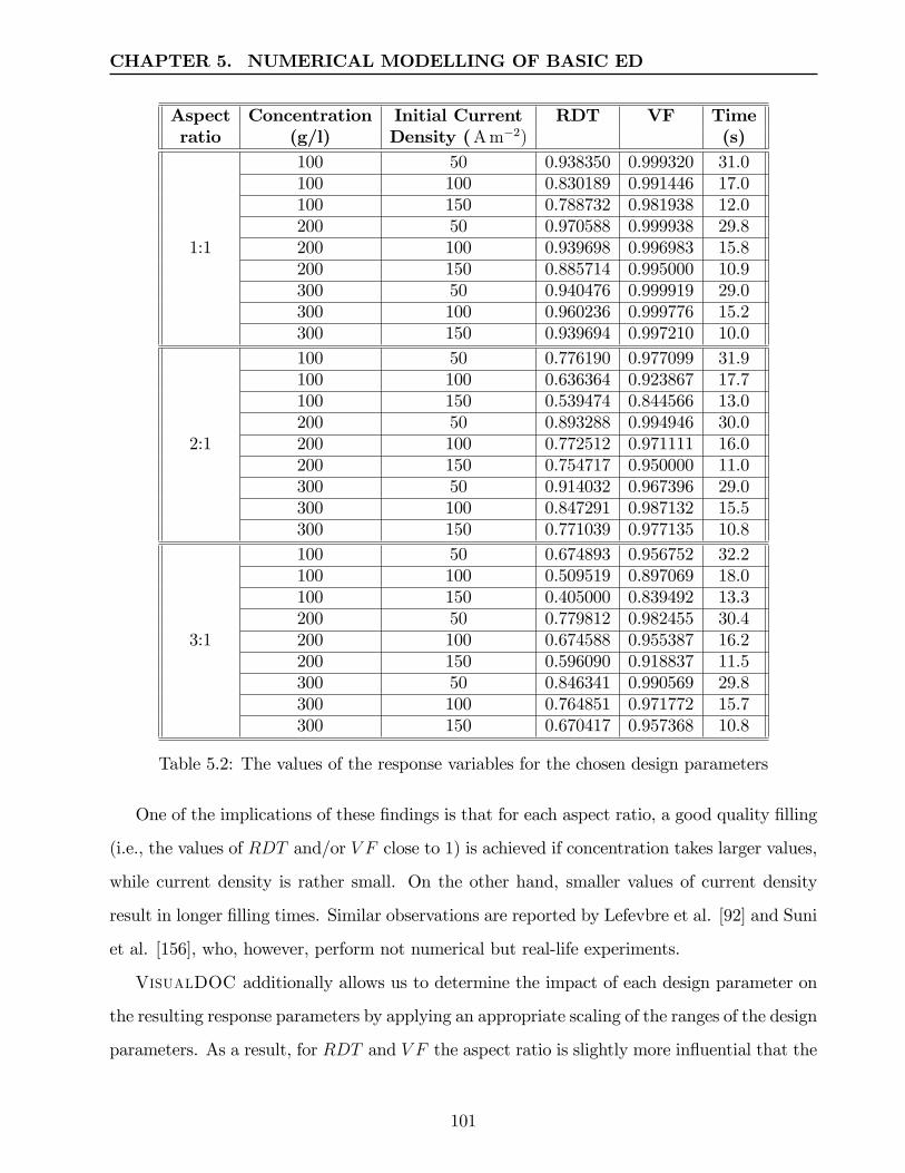
CHAPTER 5. NUMERICAL MODELLING OF BASIC ED
Aspect Concentration Initial Current RDT VF Timeratio (g/l) Density (A m−2) (s)
100 50 0.938350 0.999320 31.0100 100 0.830189 0.991446 17.0100 150 0.788732 0.981938 12.0200 50 0.970588 0.999938 29.8
1:1 200 100 0.939698 0.996983 15.8200 150 0.885714 0.995000 10.9300 50 0.940476 0.999919 29.0300 100 0.960236 0.999776 15.2300 150 0.939694 0.997210 10.0100 50 0.776190 0.977099 31.9100 100 0.636364 0.923867 17.7100 150 0.539474 0.844566 13.0200 50 0.893288 0.994946 30.0
2:1 200 100 0.772512 0.971111 16.0200 150 0.754717 0.950000 11.0300 50 0.914032 0.967396 29.0300 100 0.847291 0.987132 15.5300 150 0.771039 0.977135 10.8100 50 0.674893 0.956752 32.2100 100 0.509519 0.897069 18.0100 150 0.405000 0.839492 13.3200 50 0.779812 0.982455 30.4
3:1 200 100 0.674588 0.955387 16.2200 150 0.596090 0.918837 11.5300 50 0.846341 0.990569 29.8300 100 0.764851 0.971772 15.7300 150 0.670417 0.957368 10.8
Table 5.2: The values of the response variables for the chosen design parameters
One of the implications of these findings is that for each aspect ratio, a good quality filling
(i.e., the values of RDT and/or V F close to 1) is achieved if concentration takes larger values,
while current density is rather small. On the other hand, smaller values of current density
result in longer filling times. Similar observations are reported by Lefevbre et al. [92] and Suni
et al. [156], who, however, perform not numerical but real-life experiments.
VisualDOC additionally allows us to determine the impact of each design parameter on
the resulting response parameters by applying an appropriate scaling of the ranges of the design
parameters. As a result, for RDT and V F the aspect ratio is slightly more influential that the
101

CHAPTER 5. NUMERICAL MODELLING OF BASIC ED
Figure 5.14: Experiment 5.3: measured values of completion time (red dots) and the responsesurface (blue line)
other two design parameters, and the metric decreases as the AR increases. Concentration and
current density have almost equal quantitative impact, but the directions of their influence are
opposite: the metric grows as concentration increases and the current density decreases. As
far as the filling time is concerned, current density is clearly most influential and as it increases
the time decreases.
Our modelling results demonstrate that increasing the initial current density reduces the
electrodeposition time, but results in a greater spatial nonuniformity of the current density
which, in turn, leads to a lower quality of deposition. A similar effect has been observed in
[65], where a parametric study of ED in trenches with a conducting base (LIGA process) is
performed using the electrodeposition module of COMSOL Multiphysics 3.5a. The design
parameters have been the applied voltage, the trench geometry and trench spacing, while the
response parameters have been the overplating amount and the filling time.
The results of Experiment 5.5 can be used to develop a design optimisation and prediction
tool. Below, we give a brief description of a possible approach to creating such a tool.
Suppose that the user wants to determine the optimal values of concentration and current
density to achieve the desired values of the V F metric, between 0.9 and 1, for a 2:1 AR trench.
See Figure 5.15 for the corresponding response surface.
For each chosen value of the metric V F , it is possible to determine the optimal values of
102
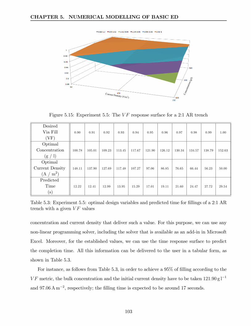
CHAPTER 5. NUMERICAL MODELLING OF BASIC ED
Figure 5.15: Experiment 5.5: The V F response surface for a 2:1 AR trench
DesiredVia Fill 0.90 0.91 0.92 0.93 0.94 0.95 0.96 0.97 0.98 0.99 1.00
(VF)Optimal
Concentration 100.78 105.01 109.23 113.45 117.67 121.90 126.12 130.34 134.57 138.79 152.63
(g / l)Optimal
Current Density 148.11 137.90 127.69 117.48 107.27 97.06 86.85 76.65 66.44 56.23 50.00
(A / m2)PredictedTime 12.22 12.41 12.99 13.95 15.29 17.01 19.11 21.60 24.47 27.72 29.54
(s)
Table 5.3: Experiment 5.5: optimal design variables and predicted time for fillings of a 2:1 ARtrench with a given V F values
concentration and current density that deliver such a value. For this purpose, we can use any
non-linear programming solver, including the solver that is available as an add-in in Microsoft
Excel. Moreover, for the established values, we can use the time response surface to predict
the completion time. All this information can be delivered to the user in a tabular form, as
shown in Table 5.3.
For instance, as follows from Table 5.3, in order to achieve a 95% of filling according to the
V F metric, the bulk concentration and the initial current density have to be taken 121.90 g l−1
and 97.06 A m−2, respectively; the filling time is expected to be around 17 seconds.
103

Chapter 6
Micro and Macro Models of FlowPhenomena in a Plating Cell
As pointed in Chapters 2 and 5, basic electrodeposition that uses no additives or any other
form of enhancement does not guarantee acceptable quality of filling of microvias. The crucial
reason of this underperformance is that basic ED does not provide a suffi cient level of ion
transport in vias. In the remaining part of this thesis, we study a possibility of enhancing the
ED process by applying a forced flow in the electrolyte.
We distinguish between flow that is induced by certain mechanical means, such as pumping,
and flow that results from megasonic agitation. This chapter focuses on numerical modelling
of relevant flow phenomena of non-acoustic nature. The material of this chapter corresponds
to Objective 4 of the thesis set in Section 1.1. The models that involve acoustically induced
flow, i.e., acoustic streaming, are considered in Chapter 7.
In this chapter, we do not consider the process of electrodeposition as such, but study the
flow phenomena that may affect the quality of electrodeposition. We have to deal with models
of several scales: on the macro level (a plating cell, with the distances measured in metres)
and on the micro level (the interior of the via, with the distances measured in microns).
Below we present a two-stage methodology for handling multi-scale flow phenomena in a
plating cell. The macro models are used to determine concentration, velocity and/or pressure
distributions in the relevant regions of the plating cell. These characteristics are taken as an
input for the micro models that study the flow characteristics inside the microvias. If the
micro model reports unsatisfactory ion transport, this produces a recommendation of looking
104

CHAPTER 6. MICRO AND MACRO MODELS OF FLOW PHENOMENA
for an alternative design of the cell.
6.1 Governing Equations and Principles of Flow Mod-elling
The mathematical and numerical models of flow phenomena belong to the most studied areas
of applied mathematics. In this section, we mainly follow the monographs [37] and [54] to
review the relevant concepts and equations.
The purpose of numerical modelling of flow is to determine a velocity distribution, rep-
resented by a function U(x, y, z, t), and/or pressure distribution, represented by a function
P (x, y, z, t), based on given initial parameters, material properties and boundary conditions,
In this chapter, we are mainly concerned with finding the velocity distribution of flow in an
incompressible liquid of a constant density ρ.
Based on the value of Reynolds number Re, two types of flow are distinguished: laminar
(if Re < 2300) and turbulent (if Re > 4000) .
The governing equations for flow can be derived from the general transport equation (4.1)
and the continuity equation (4.2) presented in Section 4.1. Replacing the abstract variable ψ
by U and taking into account that ρ is constant, we obtain the required governing equations
as
ρ∂(U)
∂t+ ρ (U · ∇)U = SU ; (6.1)
∇ ·U = 0. (6.2)
We refer to equations (6.1) and (6.2) as the momentum conservation equation and the
mass conservation equation, respectively.
For the turbulent flow the momentum conservation equation (6.1) takes the form of
ρ∂U
∂t−∇ ·
[(µ+ ρ
Cµk2
σkε
)· (∇U + (∇U)T )∇k
]+ ρU · ∇U +∇P = 0,
where µ is the dynamic viscosity, k is the turbulent energy, ε represents the dissipation rate
of turbulence energy, and Cµ is a model constant.
In order to find a solution in the case of the turbulent flow, the two main equations are
supplemented with a turbulence model. The most commonly model used for this purpose
105

CHAPTER 6. MICRO AND MACRO MODELS OF FLOW PHENOMENA
is the k − ε model, which belongs to the class of two-equation model. The k − ε model is
known to provide robustness and reasonable accuracy for a wide range of turbulent flows. It
is implemented in most popular pieces of CFD software, including PHYSICA, PHOENICS
and COMSOL.
In the k − ε model, turbulent energy k and dissipation rate ε are defined by the following
equations
ρ∂k
∂t+ ρU · ∇k = ∇ ·
[(µ+ ρCµ
k2
εσk
)∇k]
+1
2ρCµ
k2
ε
[∇U + (∇U)T
]2
− ρε
ρ∂ε
∂t+ ρU · ∇ε = ∇ ·
[(µ+ ρCµ
k2
εσε
)∇ε]
+1
2ρCε1k
[∇U + (∇U )T
]2
− Cε2ρε2
k,
The model constants in the above equations are empirical and are defined from the exper-
imental data as
Cµ = 0.09, C1ε = 1.44, Cε2 = 1.92, σk = 1.0, σε = 1.3.
The turbulent viscosity is then defined as
νt = Cµk2
ε.
Boundary conditions are introduced as the velocity at the inlet and a zero constant pressure
at the outlet. For the laminar flow, the non-slip wall boundary conditions are applied. In
the case of the turbulent flow, logarithmic wall functions at the solid walls are introduced.
The latter conditions state that the average velocity of a turbulent flow at a certain point is
proportional to the logarithm of the distance from that point to the wall, or to the boundary
of the fluid region.
For a flow along a surface, let U0 denote the mainstream velocity generated by the inlet.
According to [43], the thickness of a hydrodynamic boundary layer δFlow is defined as the
distance from the wall at which the flow velocity U becomes 99% of U0. For a laminar flow,
an estimation
δFlow = 4.91
√νx
U0
,
is accepted, where ν is the kinematic viscosity and x is the distance downstream from the start
of the boundary layer. For a turbulent flow,
δFlow ≈0.382x
Re1/5.
106

CHAPTER 6. MICRO AND MACRO MODELS OF FLOW PHENOMENA
Since the ultimate goal of this chapter is to study a possible enhancement of ion transport
in microstructures, we are not only interested in finding traditional flow characteristics such
as velocity and/or pressure distribution, but also want to determine, where possible, a distri-
bution of concentration of the metal (copper) ions carried by the flow. This can be achieved
in two steps: (i) finding the velocity/pressure field as a result of a steady state simulation of a
flow model, and (ii) taking the found distributions as boundary conditions, perform transient
simulations to solve numerically equation (4.1) with ψ representing concentration C. Moni-
toring the concentration values in all time steps at the outlet, we may also find the residence
time, which is the time the particle remains in the cell from its arrival until it leaves through
the outlet. In other words, the residence time is an indicator of how long a particle remains in
the plating cell and therefore becomes an important pointer toward the effectiveness of design
of the cell.
Finding numerical solutions to the equations for laminar and turbulent flow is the main
topic of Computational Fluid Dynamics (CFD), which we have briefly discussed in Chapter 4.
Recall that for solving the CFD problems numerous pieces of software are available, including
PHYSICA, COMSOL Multiphysics and PHOENICS. In this thesis, in our numerical
experiments with flow we mainly use the two latter packages.
6.2 A Methodology of Multi-Scale Flow Modelling
In this section, we outline a methodology that can be used for studying flow phenomena that
take place at different levels in the plating cell. Recall that here we do not consider the ED
process, but study the conditions created by flow phenomena which may favourably affect ion
transport.
A typical plating cell suitable for our purposes is shown in Figure 6.1. This particular cell
is used by our industrial project partners at Merlin Circuit Technology Ltd. Without giving
its exact specifications, here just notice that a cell is a rather large bath filled with electrolyte.
The two rails at its top are used to support panels, i.e., PCBs with predrilled microvias. A cell
is equipped with an inlet and an outlet for pumping the electrolyte. A plating cell is such a
piece of hardware that allows a limited number of alternative designs. For example, we cannot
107

CHAPTER 6. MICRO AND MACRO MODELS OF FLOW PHENOMENA
Figure 6.1: A photo of a plating cell used at Merlin Circuit Technology Ltd.
change neither the dimensions of the bath, nor the position of an outlet, which is essentially a
hole in the bottom part of the cell. What can be changed, are the number of the inlets, their
positions and/or their characteristics such as the flow rate.
One of the tasks of our methodology is to study possible designs of the plating cells/baths
with a purpose of determining their characteristics that would create conditions favourable for
electrodeposition processes enhanced by the forced flow. The use of numerical modelling at this
level allows us to test various setups and engineering ideas before their actual implementation
and to come up with the most recommended configuration of the cell. A principal scheme of
the methodology is shown in Figure 6.2.
The macro-scale model finds numerically flow characteristics in the whole cell. Because of
the scale difference, at this stage the inserted PCBs are seen as solid panels, with any predrilled
vias disregarded. The output parameters of the macro model that are of interest within the
methodology include:
• velocity/pressure distribution either at the entire inserted panel or at its predefined
region;
• concentration distribution either at the entire inserted panel or at its predefined region;
108

CHAPTER 6. MICRO AND MACRO MODELS OF FLOW PHENOMENA
Figure 6.2: A principal scheme of methodology of multi-scale flow modelling in a plating cell
• residence time.
For the macro model, as a rule we are faced with the turbulent flow, therefore for the pur-
pose of numerical modelling the turbulent flow module of the corresponding pieces of software
(COMSOL Multiphysics or PHOENICS) is engaged.
The micro-scale model takes the output of the preceding macro model as the input, e.g.,
as boundary conditions. At this stage, we perform numerical modelling of flow inside a micro
via, therefore we need the macro model to supply the relevant values in the vicinity of the via
(flow velocity at neighbourhood of the via’s mouth, bulk concentration above the via, etc.)
The output parameters of the micro model that are of interest include velocity/pressure
distribution and ion concentration distribution inside the via. Due to the size of the via, the
flow inside it is laminar. The simulations of micro models allow us to establish a flow pattern (a
through flow, single vortex, several vortices, etc.). Undesirable features that may be observed
at the micro level include insuffi cient flow penetration depths, a non-uniform concentration in
the via. Under these conditions, a subsequent electrodeposition process is unlikely to result
into a high quality filling. If any of these undesirable effects are reported, it makes sense to
109

CHAPTER 6. MICRO AND MACRO MODELS OF FLOW PHENOMENA
consider an alternative design of a cell.
Among the advantages of the outlined methodology are the following:
• it decomposes the overall problem into stages in accordance with their scale
• there is an interaction between different stages in the form of input/output and feedback
• the methodology is pure numerical.
The latter advantage is of special importance. First, numerical modelling is highly cost
effective and allows to verify various designs of the cell without making expensive real-life
prototypes. On a micro level, it allows us to monitor variations of the ion concentration on the
cathode surface (the walls and, possibly, the bottom of the via), which may heavily influence the
electroforming process. In practical application of electroforming in HAR microstructures no
monitoring instrument is able to detect the ion concentration variation in such small volumes,
thus handling this problem numerically is the only available approach.
Although the main area of application of the described methodology is related to deter-
mining conditions that are favourable for ED, it is also applicable to the initial stages of the
electroforming process, namely during the forming of a continuous conductive seed layer. Re-
call that a seed layer is normally deposited by electroless means to be used in the main stage
of ED as a cathode; see Section 2.1. Vias without a suffi cient seed layer cannot be filled fully,
as shown in Figure 6.3, where the red arrow points at the non-filled area at the bottom of the
trench with no seed layer. A study of the flow circulation of the electrolyte and/or the seed
conductive material, prior to electroplating would therefore be useful to understand the limits
of full via filling. A discussion of the use of flow techniques for creating a seed layer can be
found in [32].
In the remaining sections of this chapter, we give details of implementation and analysis of
macro-scale and micro-scale models.
6.3 Macro Models of Flow in a Standard Plating Cell
In this section, we report the results of numerical experiments with a macro-scale flow model
for a plating cell of a standard configuration that is used by our project partners at Merlin
110

CHAPTER 6. MICRO AND MACRO MODELS OF FLOW PHENOMENA
Figure 6.3: A photograph of a 3:1 AR blind via filled with copper (Courtesy of MISEC, Schoolof Engineering and Physical Sciences, Heriot-Watt University, Edinburgh)
Circuit Technology Ltd; see Figure 6.1.
Schematically, the standard plating cell is shown in Figure 6.4. The bath is a rectangular
parallelepiped of dimensions L×W ×H = 1.12 m× 0.51 m× 0.66 m. Two rectangular panels
of 0.61 m × 0.46 m are inserted in the middle of the cell. These panels are essentially PCBs,
where the micro vias are drilled. For the purpose of macro-scale numerical modelling, these
vias are ignored and the thickness of the each panel is taken to be 5 mm. Figure 6.4 also
shows the positions of the inlet and the outlet, each of size 2.54 cm× 2.54 cm. The electrolyte
is pumped through the inlet into the cell. It is known that four bath volumes are changed
during 1 hour, which corresponds to the mass flow rate on the inlet of 0.417 kg s−1 and the
inlet velocity V = 0.645 m s−1. This allows us to compute Reynolds number Re = 16383, i.e.,
the resulting flow in the cell is turbulent and can be modelled using the k− ε model described
in Section 6.1.
As mentioned in [54], the k − ε model for numerical simulations of a turbulent flow is
applicable if small gradients of velocity/pressure are observed. It appears to be suitable for
the flow modelling in plating cells, where a fairly large pressure difference occurs only in a
small region, in the vicinity of the inlet.
In accordance with the methodology outlined in Section 6.2, we need to determine the
distributions of flow velocity/pressure on the sides of the panels. We are also interested in
determining whether these distributions are suffi ciently homogeneous, i.e., how well the av-
111

CHAPTER 6. MICRO AND MACRO MODELS OF FLOW PHENOMENA
Figure 6.4: Standard plating cell with two 0.61 m × 0.46 m immersed panels: (a) front view,(b) side view, (c) top view, (d) 3D view
112

CHAPTER 6. MICRO AND MACRO MODELS OF FLOW PHENOMENA
Front view Back viewCol 1 Col 2 Col 3 Col 4 Col 1 Col 2 Col 3 Col 4
Row 1 1 2 3 4 Row 1 4 3 2 1Row 2 5 6 7 8 Row 2 8 7 6 5Row 3 9 10 11 12 Row 3 12 11 10 9Row 4 13 14 15 16 Row 4 16 15 14 13Row 5 17 18 19 20 Row 5 20 19 18 17Row 6 21 22 23 24 Row 6 24 23 22 21
Table 6.1: 24 subpanels, front and back views
erage velocity and/or pressure measured over the whole side of a panel represents similar
characteristics of selected smaller regions of the panel.
To determine these values we have performed numerical 3D simulations using COMSOL
Multiphysics based on the turbulent flow module. The mesh used for the computational
domain in Figure 6.4 consists of 3D elements with a maximum side that varies from 7 mm (for
the inlet and outlet regions) to 30 mm.
In this section, we mainly discuss the velocity distribution found by the macro model for
each side of a panel; the distribution of pressure or concentration can be treated similarly. The
output of the macro model contains an array that for each mesh element gives the velocity
value. Using a statistical terminology, such an array can be viewed as a population, that is
characterised by a mean µ (the average velocity) and a standard deviation σ. See [14] for
definitions and background of statistical techniques. A standard deviation is good measure of
variability for data, and we are interested in its estimation.
For this purpose, we split each panel into 24 identical rectangular subpanels, as schemat-
ically shown in Table 6.1. Notice that we number the subpanels row-wise from the top-left
corner of the front side, thus for the back view the numbers in each row appear in the reverse
order.
For each side, we find the average velocities on all subpanels and use these values to
estimate the population standard deviation σ and to predict the population mean µ. The
latter value can be compared to the average velocity on the whole side, which can be found
numerically. We may interpret the 24 velocity values as a sample drawn from the corresponding
population, since using the technique similar to that outlined below we can prove that with
113

CHAPTER 6. MICRO AND MACRO MODELS OF FLOW PHENOMENA
a high probability each subpanel contains an element with the velocity virtually equal to the
average velocity on that subpanel.
A formal statement of our experiments is as follows.
Experiment 6.1
Purpose: To determine velocity distribution on each side of the 24 subpanels, estimate the
standard deviation and to determine the average velocity values on each side of both panels
Domain: See Figure 6.4 with subpanels as in Table 6.1
Input Parameter: Inlet flow rate 0.417 kg s−1
Output Parameters: velocity distributions and the results of statistical analysis.
Having run a steady state simulation in COMSOL Multiphysics, we have performed
numerical integration of velocities over each side of all subpanels, as well as over the sides of
the two entire panels. Figure 6.5 shows the visual representation of the computed values. The
bar charts in the left column of Figure 6.5 are drawn in the same scale, giving a true impression
of the quantitative characteristics of velocity. In general, the profile of average velocities on
subpanels is in good agreement with the velocity distribution over the corresponding surface
(in the right column of Figure 6.5). The only noticeable exception is Row 6 of Figures 6.5(c)
and (g). This row refers to the bottom areas of the back sides of Panels 1 and 2, respectively.
As seen from Figures 6.5(d) and (h), the velocity reaches its maximum close to the bottom
of the panels, and immediately higher it takes the smallest values across the whole field. The
average velocities computed over fairly large areas fail to capture this diffi cult pattern. This
is only to be expected, given the nature of average velocity.
For each side of Panels 1 and 2 Figure 6.6 shows a histogram that indicates how many
subpanels have average velocities in a certain interval. It can be seen that in each case for at
least two thirds of subpanels the average velocities fall into a rather small interval:
• Panel 1 front: 16 subpanels in [0, 0.02] ;
• Panel 1 back: 17 subpanels in [0.09, 0.012] ;
• Panel 2 front: 16 subpanels in [0, 0.02] ;
114

CHAPTER 6. MICRO AND MACRO MODELS OF FLOW PHENOMENA
Figure 6.5: Experiment 6.1: Average velocities on subpanels (left) and velocity distributionon full panels (right); Panel 1 front (a, b), Panel 1 back (c, d), Panel 2 front (e, f), Panel 2back (g, h)
115

CHAPTER 6. MICRO AND MACRO MODELS OF FLOW PHENOMENA
Figure 6.6: Experiment 6.1: Frequency distributions of average velocities
• Panel 2 back: 19 subpanels in [0.006, 0.012] .
We have subjected the collected data to a standard statistical analysis [14]. The derived
results are tabulated in Table 6.2. The population standard deviation σ is estimated as S/√
24.
Since the size of the sample is 24 < 30, to find the confidence intervals for the population mean
µ, we use the t−test with t0.005,23 = 2.808, which allows to determine the intervals with a high
probability of 99.5%. With the significance level of α = 1% we cannot reject a hypothesis that
the population mean and the sample mean coincide.
Observe that we make a very good prediction of the population mean µ, which is close
to the sample mean X. Considering the population standard deviation σ as a measure of
diversity of velocities on each side, it can be seen that the velocity field on the back of both
panels is fairly uniform, with σ = 0.4 mm s−1 and σ = 0.7 mm s−1, which is in good agreement
with Figure 6.5(d) and (h) and the histograms in Figure 6.6.
For the front side of Panel 2 the value of σ is the largest, and the mean velocity
116

CHAPTER 6. MICRO AND MACRO MODELS OF FLOW PHENOMENA
Panel 1 Panel 1 Panel 2 Panel 2Front Back Front Back
Average velocity, 0.0181 0.0109 0.0228 0.0102sample mean XSample standard 0.0104 0.0020 0.0180 0.0032deviation SEstimated population 0.0021 0.0004 0.0037 0.0007standard deviation σConfidence interval [0.0122, 0.0241] [0.0097, 0.0120] [0.0124, 0.0331] [0.0084, 0.0121]for population mean µNumerically found 0.0180 0.0107 0.0232 0.0103average velocity µ
Table 6.2: Experiment 6.1: Results of statistical analysis, all values are in m/s
X = 0.0228 m s−1 or µ = 0.0232 m s−1 does not belong to the interval [0, 0.02] of the high-
est frequency, see Figure 6.6. From these observations we derive that the velocity field over
this surface is highly non-uniform, which also is confirmed by Figure 6.5. This lack of homo-
geneity can be explained by the proximity of the panel to the inlet and/or outlet. To achieve
a more uniform velocity field, changes to the cell’s setup can be recommended.
6.4 Comparing Macro Models for Different Cell Designs
In this section, we compare the macro model based on the cell design described in Section 6.3
and the model for the cell of an alternative design. We refer to these two designs of a cell as
Design 1 and Design 2. The difference between the two designs is in the position of the inlet:
for Design 2 the inlet is moved from the left front corner (see Figure 6.4) to the top middle at
the front wall of the cell (see Figure 6.7).
In accordance with the general methodology shown in Figure 6.2, we perform comparisons
of the two design, so that the decision-makers can select the design that is most suitable
for their purposes, or if none of the designs suits well enough, an additional design can be
introduced and analysed.
The feature of a design that should be seen as positive is homogeneity of veloc-
ity/pressure/concentration distribution on the surfaces of the panels. Recall that an ultimate
goal of a good cell design is to guarantee a good ion transport to and inside micro vias. There-
117

CHAPTER 6. MICRO AND MACRO MODELS OF FLOW PHENOMENA
Figure 6.7: Alternative cell design: (a) front view; (b) 3D view
fore, the influence of other characteristics of the design obtained at the macro level strongly
depends on the type of microstructures involved at the micro level. Some of these factors are
listed below.
Through vias: As will be shown in Section 6.6, good ion transport is provided if there is a
considerable difference in velocity or pressure (velocity or pressure drop) on the sides of
a panel.
Blind Vias: As will be shown in Section 6.5, the larger velocity at the mouth region of the
via, the better ion transport inside the via is observed.
Below, comparing macro models for Design 1 and Design 2, we pay attention to all men-
tioned characteristics, and additionally we compare the residence times and the dynamics of
concentration distributions.
Figure 6.8 shows the velocity distributions over the surfaces of the panels in a cell of Design 2
found by running simulations using COMSOL Multiphysics. By visual comparison of this
figure with Figure 6.5 we notice that
• For Design 2 the distributions over the back surfaces are more uniform than for Design 1;
• For Design 2, the distributions over the front surfaces follow a pattern that is almost
symmetric with respect to the central position of the inlet;
• For Design 2, the distribution over the front surface of Panel 1 is less uniform than for
118

CHAPTER 6. MICRO AND MACRO MODELS OF FLOW PHENOMENA
Figure 6.8: Velocity distributions for Design 2: (a) Panel 1 front; (b) Panel 2 front; (c) Panel1 back; (d) Panel 2 back
Design 1, but that is compensated by a more even distribution over the front surface of
Panel 2.
These observations can be verified statistically. For this purpose, we determine character-
istics of the macro model for Design 2 by the same technique as described in Section 6.3, i.e.,
splitting each side of each panel into 24 subpanels, as shown in Table 6.1.
For each side of Panels 1 and 2 Figure 6.9 shows a histogram that indicates how many sub-
panels have average velocities in a certain interval. As expected, the histograms in Figures 6.6
and 6.9 show different profiles. However, as in the case of Design 1, for at least two thirds of
subpanels in the cell of Design 2 the average velocities fall into a rather small interval:
• Panel 1 front: 17 subpanels in [0, 0.03] ;
• Panel 1 back: 17 subpanels in [0.08, 0.012] ;
• Panel 2 front: 18 subpanels in [0, 0.02] ;
• Panel 2 back: 17 subpanels in [0.003, 0.012] .
119

CHAPTER 6. MICRO AND MACRO MODELS OF FLOW PHENOMENA
Figure 6.9: Frequency distributions of average velocities for Cell 2
Table 6.2 shows the results of standard statistical analysis for the data collected for Design 2.
As for Design 1 (see Table 6.2), here again we see that the numerically found average veloc-
ities are very close to the sample mean values. Comparing the estimated standard deviations,
we see that for Design 2 the velocity distributions for both back surfaces of the panels are
rather uniform. The front surface of Panel 2 is considerably more homogeneous than that of
Design 1, with a considerable drop in standard deviation from 0.0037 m s−1 to 0.0024 m s−1.
On the other hand, we deduce that for Design 2 the velocity distribution over the front surface
Panel 1 Panel 1 Panel 2 Panel 2Front Back Front Back
Average velocity, 0.0236 0.0094 0.0203 0.0087sample mean XSample standard 0.0128 0.0021 0.0117 0.0038deviation SEstimated population 0.0026 0.0004 0.0024 0.0006standard deviation σNumerically found 0.0237 0.0095 0.0199 0.0087average velocity µ
Table 6.3: Results of statistical analysis for Design 2, all values are in m/s
120

CHAPTER 6. MICRO AND MACRO MODELS OF FLOW PHENOMENA
Confidence interval for µ2 − µ1 Confidence interval for µ2 − µ1
(front surfaces) (back surfaces)Design 1 −0.0067 ≤ µ2 − µ1 ≤ 0.0161 −0.0027 ≤ µ2 − µ1 ≤ 0.0014Design 2 −0.0128 ≤ µ2 − µ1 ≤ 0.0062 −0.0031 ≤ µ2 − µ1 ≤ 0.0017
Table 6.4: Confidence intervals for the differences of average velocities (in m/s)
of Panel 1 is slightly more uneven than in the case of Design 1.
For a particular design, let µ1 and µ2 denote the average velocities over the corresponding
surfaces of Panel 1 and Panel 2 (either two front surfaces or two back surfaces). Another
statistical measure that also allows us to judge the uniformity of the velocity distributions is
to statistically estimate the difference µ2−µ1 over the two front surfaces and two back surfaces.
Using the method of estimating the difference of population means in the case of small samples
[14], with probability 99.5% we have found the confidence intervals presented in Table 6.4.
It can be seen that for the front surfaces the range of values for µ2 − µ1 is 22.8 mm s−1
for Design 1 and 19.0 mm s−1 for Design 2, i.e., with a high probability we expect a larger
non-uniformity between the front surfaces of the panels in Design 1. For the back surfaces, the
ranges are 4.1 mm s−1 and 4.8 mm s−1, which means for both designs there is no big difference
between velocities over the back surfaces of the panels.
Another characteristics of effectiveness of a cell design that can be derived from the macro
model are the residence time and the concentration distribution. As described in Section 6.1,
for determining these parameters we run two-step 3D simulations. In the first step, as a result
of a steady state simulation we obtain the velocity field. In the second step, using this field as
a boundary condition, we perform a transient simulation to solve numerically equation (4.1)
with ψ representing concentration C. We are interested in relative values of concentration,
i.e., its initial value is immaterial and we nominally set it as CInlet = 1. The residence time is
determined by monitoring the concentration at the outlet. In our experiments the transient
simulations cover the period of 1 h, with a time step of 1 s.
In order to achieve a required accuracy, especially for finding the residence time, we need
to use a rather fine 3D mesh. In principle, it is possible to use COMSOL Multiphysics
for these purposes, which gives an additional advantage of an extensive postprocessing toolkit
(integrating the decision variables over prescribed domains and boundaries). However, due
121

CHAPTER 6. MICRO AND MACRO MODELS OF FLOW PHENOMENA
Figure 6.10: Residence time for Design 1 and Design 2
to its rather universal nature, the 3D transient simulation in COMSOL Multiphysics for
computing the residence time may take several days of the CPU time. Thus, we have given
preference to PHOENICS as a specialised CFD software, which is capable to deliver the
required solution in a reasonable time.
In Figure 6.10, the vertical axis C/CInlet represents the proportion of particles at the outlet
compared to the number of particles that enter the cells through the inlet. The actual residence
time is the time at which C/CInlet = 1, i.e., all arrived particles have left the cell. Instead of
computing the actual residence time, we present the dynamic change of C/CInlet during 1 h. It
can be seen that in the case of Design 1, 80% of particles leave the domain in 15 min, and 90%
leave in half an hour. On the other hand, for Design 2, only 60% of particles leave the domain
in 15 min, and 83% leave in half an hour. This can be attributed to the fact that in Design 1
the outlet is closer to the inlet than in Design 2. Also observe that, for Design 1, the rate of
change of C/CInlet grows rapidly in the first half an hour, and then considerably slows down.
For Design 2, there is a steady growth of the rate, and after 3000 s, C/CInlet grows faster for
Design 2 than for Design 1.
The patterns of concentration distributions for Designs 1 and 2 are shown in Figure 6.11.
We see that for Design 2 the concentration remains fairly uniform at all times, and after 1 h
122

CHAPTER 6. MICRO AND MACRO MODELS OF FLOW PHENOMENA
Figure 6.11: Top views of concentration distributions at the central vertical cross-section forDesign 1 (left column) and Design 2 (right column): (a, b) after 15 min; (c, d) after 30 min;(e, f) after 60 min
achieves a high level of 0.95 across the whole cross-section. For Design 1, already after 15 min
the concentration achieves the values close to 1 in the area that is close to the inlet and the
outlet. The area with high concentration grows as time passes by; however, in the opposite
part of the cross-section even after 1 h the concentration does not reach 0.15.
This complies well with our earlier observations that in Design 1 the two panels due to the
difference in their distances from the inlet are not in similar conditions.
6.5 Micro-Scale Models of Vias: Tangential Flow
In this section, we study the influence of the flow that is directed tangentially with respect
to the mouth of a via on the flow characteristics and ion concentration distribution inside the
via. The results of this section have been reported in [32, 33, 34].
Among the motivations for these series of experiments are the following:
• To test whether the tangential flow is capable of enhancing the ion transport in small
123
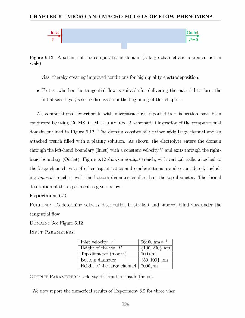
CHAPTER 6. MICRO AND MACRO MODELS OF FLOW PHENOMENA
Figure 6.12: A scheme of the computational domain (a large channel and a trench, not inscale)
vias, thereby creating improved conditions for high quality electrodeposition;
• To test whether the tangential flow is suitable for delivering the material to form the
initial seed layer; see the discussion in the beginning of this chapter.
All computational experiments with microstructures reported in this section have been
conducted by using COMSOL Multiphysics. A schematic illustration of the computational
domain outlined in Figure 6.12. The domain consists of a rather wide large channel and an
attached trench filled with a plating solution. As shown, the electrolyte enters the domain
through the left-hand boundary (Inlet) with a constant velocity V and exits through the right-
hand boundary (Outlet). Figure 6.12 shows a straight trench, with vertical walls, attached to
the large channel; vias of other aspect ratios and configurations are also considered, includ-
ing tapered trenches, with the bottom diameter smaller than the top diameter. The formal
description of the experiment is given below.
Experiment 6.2
Purpose: To determine velocity distribution in straight and tapered blind vias under the
tangential flow
Domain: See Figure 6.12
Input Parameters:
Inlet velocity, V 26400µm s−1
Height of the via, H 100, 200 µmTop diameter (mouth) 100µmBottom diameter 50, 100 µmHeight of the large channel 2000µm
Output Parameters: velocity distribution inside the via.
We now report the numerical results of Experiment 6.2 for three vias:
124

CHAPTER 6. MICRO AND MACRO MODELS OF FLOW PHENOMENA
Via A: a 2:1 AR tapered via of height 200µm with the bottom diameter 50µm;
Via B: a 1:1 AR tapered via of height 100µm with the bottom diameter 50µm;
Via C: a 1:1 AR straight via of height 100µm.
In each case, we run a steady-state simulation as a two-stage process that uses the chemical
engineering module of COMSOL Multiphysics. In the first stage, the Navier-Stokes sub-
module for incompressible fluid delivers the velocity distribution in the computational domain.
In the second phase, we rely on multiphysics capabilities of COMSOL and run the convection
and diffusion submodule, which finds the concentration distribution, taking into account the
previously found velocity field. Since we are interested in the behaviour of the concentration
distribution rather in specific actual values, for the second stage we set the initial nominal
concentration on the inlet of the large channel equal to 100 mol m−3.
Figure 6.13 shows the results obtained for Via A: the velocity vectors after the first stage
of the simulation and the concentration contours found in the second stage. It can be seen
that as the flow hits the right wall of the trench, a single vortex is formed, while the fluid in
the lower part of the trench is almost static. The vortex circulates in the clockwise direction,
i.e., the electrolyte flows over the cathode surface from the downstream to the upstream side.
The concentration distribution in Figure 6.13(b) reflects how the ions are carried by the flow
in Figure 6.13(a). We observe high concentration values in the vicinity of the top-right corner
of the trench, lower values in the top-left part of the trench and very low values at its bottom.
This implies that if an electrodeposition process was performed under the conditions of the
tangential flow, high quality filling for such a trench would not be achieved, since an asymmetric
crowding effect would be observed at the mouth of the trench and the electrolyte would get
depleted at the bottom.
Figure 6.14 shows the results obtained for Vias B and C: the velocity vectors after the first
stage of the simulations and the concentration flux streamlines drawn in red on top of the
velocity contours. Similar patterns are observed, with a vortex formed, which would affect
electrodeposition under these conditions by producing a rather asymmetric filling.
Comparing the results for Vias B and C is of interest in its own right. The two vias have
125

CHAPTER 6. MICRO AND MACRO MODELS OF FLOW PHENOMENA
Figure 6.13: Experiment 6.2, the results for Via A: (a) velocity vectors, (b) concentrationdistribution
Figure 6.14: Experiment 6.2: (a, c) velocity vectors for Vias B and C, respectively; (b,d)velocity distribution and concentration flux streamlines for Vias B and C, respectively
126

CHAPTER 6. MICRO AND MACRO MODELS OF FLOW PHENOMENA
Figure 6.15: Experiment 6.2: Velocities at the vertical central cross-section of Vias B and C
the same mouth diameter, the height and essentially the aspect ratio. Choosing the profile of a
via may have a strong impact on the quality of ED; see Section 2.1. Lefebvre et al. [92] report
on better quality filling achieved for tapered trenches, rather then for straight or barrel-shape
trenches of the same AR. However, in the case of the tangential flow above the trench a better
ion transport is observed for the straight trench, not tapered. Figure 6.15 plots the graphs
of velocities computed along the vertical central cross-section of Vias B and C. We observe
that the values are essentially the same in the top regions of both vias, rapidly decreasing
to 0 at about 30µm from the top, which corresponds to the centre of the vortex. After this
position, for each via velocity increases, which corresponds to the lower part of the vortex.
However, for the straight Via C the velocity takes larger values and penetrates deeper: for
Via B the maximum velocity of 60µm s−1 is achieved at 43µm from the top, while for Via C
the maximum velocity of 83µm s−1 is achieved at 54µm from the top. Having reached these
maximum values, the velocity decreases to zero at the bottom of the trenches, but for any
depth the velocity values for Via C are higher than those for Via B. This behaviour can be
explained by the fact that in the case of a tapered trench the incoming tangential flow hits the
reflective wall earlier than in the straight trench.
The obtained numerical results have been compared with the real-life measurements taken
by our project partners from MISEC, School of Engineering and Physical Sciences, Heriot-
Watt University, Edinburgh, who used Particle Image Velocimetry (PIV) method to analyse
127

CHAPTER 6. MICRO AND MACRO MODELS OF FLOW PHENOMENA
Figure 6.16: The microfluidic chip used for micro-PIV analysis. The position of the largechannel is shown by the dashed line
fluid flow. An optically transparent microfluidic sample has been designed to mimic the cross-
section of a PCB containing vias of various aspect ratios, as shown in Figure 6.16. The dashed
line marks the large channel, 2 mm× 60 mm, that represents the cross section of a top surface
of the PCB where the electroplating solution is placed. Cross sections of the vertical sidewalls
and various blind vias are replicated along the length of the channel. The microfluidic samples
have been fabricated by the Company Epigem Ltd, which specialises in the manufacturing of
microfluidic components based on PMMA. A fluid representing the electrolyte solution and
containing polystyrene beads of 0.4µm diameter has been passed through the microfluidic
sample and measurements have been taken using a DantecTM system that coordinates the
illumination set-up, the capturing of the images and the processing of the data.
For illustration, we compare the velocity measurements taken along the vertical cross-
section of the straight Via C and the values numerically found in Experiment 6.2; see Fig-
ure 6.17.
It can be seen, that the modelled speed of flow is fairly similar to that of the measured
micro-PIV analysis with a correlation coeffi cient of around 0.907. The speed of flow drops off
considerably as the penetration depth increases.
Both numerical and real-life experiments demonstrate that tangential flow does not enhance
the ion transport significantly. The electroplating solution is not readily refreshed at the
bottom of blind vias and the ions are depleted in this area, potentially causing electrodeposition
defects, such as void formation.
128

CHAPTER 6. MICRO AND MACRO MODELS OF FLOW PHENOMENA
Figure 6.17: Experiment 6.2: Numerical results and measured values for velocities at thevertical central cross-section of Via C
6.6 Micro-Scale Models of Flow in Through Vias
In this section, we present the results of numerical simulations of a flow in through vias, drilled
in a board. The purpose of this study is to determine the impact of a flow that is tangential to
the board on the velocity and pressure distribution inside the via. As in the previous section,
all computational experiments have been conducted by using COMSOL Multiphysics.
In the series of conducted numerical experiments, we look at the flows in the upper and
lower channels connected by the via and distinguish between two situations: (i) the flows
in both channels are of the same direction, and (ii) the flows in the upper and in the lower
channels are of the opposite directions. The computational domains for these two situations
are shown schematically in Figure 6.18. Here, the red arrows show the directions of inlet flows,
while the outlets are marked by blue lines where pressure is zero, i.e., P = 0.
These experiments have been initiated by the projects partners. The knowledge of the flow
properties inside the via would allow us to analyse the ion replenishment due to that flow. We
report the results of two series of numerical experiments, one with a HAR via, and the other
with a 1:1 AR via.
129

CHAPTER 6. MICRO AND MACRO MODELS OF FLOW PHENOMENA
Figure 6.18: Computational domains: (a) co-directional flows; (b) counter-directional flows
6.6.1 Experiments with a 10:1 AR through via
In principle, to analyse the flow inside a through via the required real-life measurements could
have been taken by using the micro-PIV technology. However, such measurements appear to
be hard to perform for HAR vias (AR 10:1 or higher) and this increases the importance of the
numerical modelling approach.
The formal statement of the experiments conducted with a HAR via is given below.
Experiment 6.3
Purpose: To determine velocity and pressure distribution in a through via of a 10:1 aspect
ratio
Domain: See Figure 6.18
Input Parameters:
Upper inlet velocity, V1 330µm s−1
Lower inlet velocity, V2 0, ± 200, ± 330 µm s−1
Height of the via, H 1000µmRadius of the via, d 50µmHeight of the upper and lower channels 2000µm
Tracking Parameters: velocity and pressure distribution inside the via
For each value of velocity V2, numerical steady state simulations have been conducted.
To report the results of these simulations, we split the interior of the via into three regions,
A, B and C, that represent the top third, the middle third and the bottom third of the via,
respectively; see Figure 6.19(a).
First, we present the values of the average velocity in the three regions, along with the
visual representations of corresponding vectors; see Table 6.5 and Figure 6.19.
130

CHAPTER 6. MICRO AND MACRO MODELS OF FLOW PHENOMENA
V2 Average Values Average Values Average Values Visualin Region A in Region B in Region C Representation
0 21.91 21.89 21.90 Figure 6.19(b)±200 8.79 8.74 8.76 Figure 6.19(c)±330 0.37 2.4× 10⁻⁴ 0.37 Figure 6.19(d)
Table 6.5: Experiment 6.3: Average velocity values (um /s)
Figure 6.19: Experiment 6.3: (a) regions of the via; values and vectors of velocity: (b) V2 = 0,(c) V2 = ±200µm/ s, (d) V2 = ±330µm/ s
131

CHAPTER 6. MICRO AND MACRO MODELS OF FLOW PHENOMENA
Below we list several observations regarding the behaviour of the average velocity inside
the via.
• In each region A, B and C, the average velocity depends on the absolute value of V2 of
the flow velocity in the lower channel, and is independent of its direction;
• If there is no flow in the lower channel, i.e., V2 = 0, the velocity reaches its maximum
and is uniform along the vertical sections of the via, see Figure 6.19(b);
• If the flow in the lower channel is slower than in the upper channel, i.e., |V2| < V1, the
flow goes through the via downwards, and at the bottom mouth the direction of the flow
is determined by the direction of the flow in the lower channel, see Figure 6.19(c);
• If |V2| = V1 then a small circulation is observed in the area close to each mouth, and the
flow is essentially absent in areas close to Region B, see Figure 6.19(d).
Consider now the pressure drop ∆P along the centre cross section of the via, which exhibits
a similar behaviour.
• The pressure drop depends on the absolute value of V2, and is independent of its direction;
• The largest pressure drop of ∆P = 0.0265 Pa is observed for the case of V2 = 0;
• For the case |V2| < V1, the pressure drop is ∆P = 0.01 Pa;
• For the case |V2| = V1, pressure remains constant P = 0.0286 Pa, no pressure drop is
observed.
The main conclusion of these series of experiments is that in order to guarantee higher
velocity values (or, equivalently, a large pressure drop) in a HAR through via, the bath design
should provide the largest possible difference between the absolute values of the flow velocities
at the two sides of the board, above and below the via.
132

CHAPTER 6. MICRO AND MACRO MODELS OF FLOW PHENOMENA
Figure 6.20: Results for the same directions of external flows: (a) velocity vectors deliveredby the PIV imaging system (b) velocity vectors found by COMSOL, (c) velocity distributionsand streamlines found by COMSOL
6.6.2 Experiments with a 1:1 AR through via
Additionally, we have conducted a similar experiment with a 1:1 AR through via, 100µm ×
100µm. Two versions of the tangential external flow of the same magnitude have been studied:
(i) the same direction in the upper and lower channels, and (ii) the opposite directions, as shown
in Figure 6.18(a) and (b), respectfully. If in Experiment 6.3 with a HAR through via the inner
flow patterns mainly depend on the magnitudes of the external flows but not on their direction,
here we have observed that the flow behaviour in the via essentially depends on the directions
of the external flows. We have conducted numerical simulations with a 1:1 AR through via
based on a similar model as in Experiment 6.3.
The numerical results in the case of the same direction in the upper and lower channels
are shown in Figure 6.20. Besides, for this case we have been able to compare our findings
with the PIV measurements performed by our partners from MISEC, School of Engineering
and Physical Sciences, Heriot-Watt University, Edinburgh; see Section 6.5 for more details.
Unlike in Experiment 6.3 with a HAR through via, here the flow inside the via forms two
fairly symmetric vortices that rotate in the opposite directions. Thus, the flow in the upper
channel will provide the ion transport in the top part of the via, while the flow in the lower
channel will be responsible for the ion supply in the bottom part. The lowest velocity is
observed in the vicinity of the walls, at the half depth of the via.
133

CHAPTER 6. MICRO AND MACRO MODELS OF FLOW PHENOMENA
Figure 6.21: Numerical results for the opposite directions of external flows found byCOMSOL:(a) velocity vectors, (b) velocity distributions and streamlines
If the flows in the upper and lower channels run in the opposite directions, the flow inside
the via exhibits a completely deferent behaviour, as can be seen in Figure 6.21.
Here, the flow inside the via forms a single vortex that rotates clockwise. This will provide
a good circulation and a more uniform ion supply to the walls’region.
One of the implications of the numerical study presented in this section is that in order to
guarantee higher velocity values in a through via, the bath design should provide the largest
possible difference between the absolute values of the flow velocities at the two sides of the
board. This provides a feedback to the macro model discussed in Section 6.3, which in turn
may lead to redesign recommendations.
6.7 Parametric Study on Micro-Scale Flow Models inTrenches
In this section, we present the results of a parametric study of micro-scale models with trenches
of various geometric configurations. The purpose of this study is to characterise flow perfor-
mance under direct flow, with the vertical velocity penetration depth and the average velocity
as the performance metrics.
In the series of conducted numerical experiments, it is assumed that a trench has the
structure as shown in Figure 6.22, where
134

CHAPTER 6. MICRO AND MACRO MODELS OF FLOW PHENOMENA
Figure 6.22: Configuration of the trenches in the parametric study
• D is the fixed top diameter;
• h is a variable height;
• d is a variable bottom diameter.
It is assumed that a two-dimensional laminar flow is applied, directed perpendicularly to
the board. The perpendicular flow orientation is known to enhance the transport of chemical
species, as observed in real-life experiments [51].
Figure 6.23 outlines the corresponding computational domain. Formally, the setup of the
study can be described as follows.
Experiment 6.4
Purpose: To characterise flow performance in trenches under direct flow
Domain: See Figure 6.23
Fixed Input Parameters:
Top diameter, D 120µmInlet flow velocity, VInlet 10−3 m s−1
Distance from the inlet to the board 100µm
135

CHAPTER 6. MICRO AND MACRO MODELS OF FLOW PHENOMENA
Figure 6.23: Computational domain for the parametric study
136

CHAPTER 6. MICRO AND MACRO MODELS OF FLOW PHENOMENA
Design Parameters:
Height of a trench, h 80, 100, 120 µmBottom diameter of a trench, d 60, 80, 100, 120 µm
Response Parameters: vertical velocity penetration depth, average velocity values in var-
ious parts of the trench (at the mouth of the trench, at the top/middle part and at the
middle/middle part); see Figure 6.24.
For each combination of the design parameters, numerical steady state simulations have
been conducted by running the Navier-Stokes module for incompressible fluid within COM-
SOL Multiphysics.
For the direct flow along the vertical symmetry axis of a trench, a similar pattern of velocity
distribution has been observed for all trenches; for illustration, see Figure 6.25 that shows the
velocity field and velocity streamlines (in red) for one of the trenches. Notice that the direct
flow initiates two symmetric vortices, with the opposite directions of rotation. Thus, the direct
flow supplies the ions to the side walls at the same rate, and therefore we may expect an even
side-wise filling of the via at the electrodeposition stage. This is in contrast with the case of
the tangential flow above the trench studied in Section 6.5, where a single asymmetric vortex
is formed, which may result into a non-uniform filling of the via during electrodeposition.
In Experiment 6.4, in order to compute the penetration depth of the flow velocity, we
consider the velocity distribution along the vertical cross-section of the trench and determine
point Q, at which the vertical component of the velocity becomes less than 10−8 m s−1; we
may assume that below Q only chaotic Brownian movement takes place; see Figure 6.24(a).
The penetration depth is reported as a ratio of the depth of Q (the distance between Q and
Figure 6.24: Computing response parameters for Experiment 6.4: (a) penetration depth; (b)the mouth of the trench; (c) the top/middle part of the trench; (d) the middle/middle part ofthe trench
137

CHAPTER 6. MICRO AND MACRO MODELS OF FLOW PHENOMENA
Figure 6.25: Experiment 6.4: Velocity distribution and streamlines for the trench with h =100µm and d = 80µm
the mouth of the trench) to the height of the trench. The average velocity is computed by
numerical integration over the relevant area; see Figure 6.24(b)-(d).
The obtained results are reported in Table 6.6.
Penetration Average Velocity Average Velocity Average Velocity ath d Depth at the Mouth at the Top/Middle the Middle/Middle
(µm) (µm) (%) (µm /s) (µm /s) (µm /s)
60 90.9 877.1 147.1 9.880 80 93.5 879.6 151.3 15.8
100 95.0 882.3 157.0 23.2120 95.5 885.6 164.0 31.3
60 83.4 878.6 149.5 13.5100 80 89.5 880.7 153.6 19.7
100 92.5 883.0 158.9 27.5120 94.0 885.7 165.4 36.6
60 74.3 879.6 152.0 16.4120 80 80.9 881.7 155.0 21.8
100 86.7 883.6 159.0 28.2120 90.8 885.8 165.6 37.2
Table 6.6: Numerical results of Experiment 6.4
The data of this table has become an input for the DoE module of VisualDOC, see
Section 4.5, and for each of the response parameters the response surface has been found, as a
quadratic approximation function of two design variables, h and d; see Table 6.7 for the found
138

CHAPTER 6. MICRO AND MACRO MODELS OF FLOW PHENOMENA
Response Response Surface Coeffi cientsParameter h2 d2 hd h d Const
Penetration depth (a) −0.0035 −0.0019 0.0050 −0.0259 0.0122 96.8040Av. velocity at mouth (b) 0 0.0003 −0.0010 0.1243 0.1591 861.0500Av. velocity at top/middle (c) −0.0012 0.0018 −0.0015 0.4443 0.0720 115.100Av. velocity at middle/middle (d) −0.0034 0.0018 0 0.8281 0.0405 −43.4780
Table 6.7: Experiment 6.4: Coeffi cients of response surfaces
Response Response DirectParameter Surface Simulation
Penetration depth (%) 77.84 77.40Av. velocity at mouth (µm/ s) 880.65 889.70Av. velocity at top/middle (µm/ s) 153.15 153.50Av. velocity at middle/middle (µm/ s) 18.60 19.50
Table 6.8: Experiment 6.4: Predicted and computed values for a specific trench
coeffi cients, rounded to 4 decimal places. The corresponding response surfaces are shown in
Figure 6.26
The obtained response surfaces fit very well to the observations listed in Table 6.6. For
example, for the penetration depth, VisualDOC outputs the coeffi cient of multiple determi-
nation R2 equal to 0.9978; the values of R2 for the average velocities for the mentioned three
areas are equal to 0.9935 (mouth), 0.9988 (top/middle) and 0.9975 (middle/middle).
VisualDOC additionally allows us to determine the impact of each design parameter
on the resulting response parameters. For the average velocities in the top/middle and mid-
dle/middle areas, h is reported to be more significant than d, while for the other two response
parameters related to average velocity we may treat h and d as equally important.
The results of Experiment 6.4 can be used to develop a prediction tool. For example,
our partners at Merlin Circuit Technology Ltd are in particular interested in a trench with
D = 120µm, h = 120µm and d = 70µm. For this trench, Table 6.8 shows the values of the
four response parameters found by substitution into the analytical expressions from Table 6.7,
as well as those computed as a result of a direct numerical simulation.
The predicted and computed values fit extremely well, with R2 = 0.999998.
Briefly, the results of Experiment 6.4 with the direct flow in the trenches of the fixed top
diameter D can be stated as follows.
139

CHAPTER 6. MICRO AND MACRO MODELS OF FLOW PHENOMENA
Figure 6.26: Response surfaces for response parameters: (a) penetration depth; (b) averagevelocity at the mouth; (c) average velocity at the top/middle area; (d) average velocity at themiddle/middle area
140

CHAPTER 6. MICRO AND MACRO MODELS OF FLOW PHENOMENA
• For a fixed height h, the decrease in the bottom diameter d results into a decrease of the
values of all four response parameters.
• For a fixed bottom diameter d, the decrease in height h results into a decrease of all three
response parameters related to average velocity, while the penetration depth increases.
Thus, in the presence of the direct flow, the straight vias are preferable, as far as the ion
transport is concerned. Notice that a similar conclusion is derived in Section 6.5, for the case
of the tangential flow.
141

Chapter 7
Micro and Macro Models of AcousticAgitation
Megasonic agitation is accepted as a possible mechanism of enhancing basic electrodeposition
with a purpose of producing high quality fillings of microvias.
Similar to Chapter 6, here we also face with both macro and micro models of the acoustically
induced phenomena, and we develop the corresponding two-stage methodology. The macro
models are used to determine a possible additional flow in the plating cell. Besides, for the
region of the mouth of a microvia, macro models supply the amplitude of the acoustic velocity
and guarantee a high level of ion concentration. At the micro level, we determine that the
latter factor has the most significant influence on ion transport. On the other hand, taking
into account acoustic streaming inside the via is demonstrated to lead to no improvements
for blind vias and to a minor improvement for through vias. The experiments with numerical
models that combine both basic ED and AS are reported and analysed. The material of this
chapter corresponds to Objective 6 of the thesis set in Section 1.1.
7.1 Review of Approaches to Modelling of AcousticPhenomena
In Chapter 3, we have described the general principles of mathematical modelling of acoustic
streaming based on the method of successive approximations. This general technique has been
illustrated for various situations, including standing/traveling waves, open/closed channels,
slip/non-slip wall boundary conditions, etc. In this section, we review more recent develop-
142

CHAPTER 7. MICRO AND MACRO MODELS OF ACOUSTIC AGITATION
ments in this area, paying attention not only to the mathematical side of modelling, but also to
possible approaches to finding numerical solutions of relevant problems. Recall that notation
and definitions of the variables related to acoustic streaming (AS) are given in Table 2.
Multiple attempts have been made to find a general solution for the relationship between
the intensity field and the acoustic velocity, taking into account streaming effects.
Tjotta [160] introduces a simple formula for the streaming velocity
Us =8αIR2
µc. (7.1)
Starritt et al. [152] calculate the velocities using this formula for typical beams applied in
Doppler sonography. However, as shown in [152], the experimentally measured velocities may
considerably differ from those computed by (7.1).
Wu and Du [175] develop an approximate solution for the on-axis AS velocity generated
by a flat and weakly focused transducer. They use the method of successive approximations
and time averaging to derive the governing stream equation that is accurate up to the second
order. Applying the parabolic approximation method by Aanonsen et al. [1], the authors
obtain that Ua ' Paρ0c, and further they derive the Poisson equation for the axial streaming
velocity ∇2Us = −2αµcIx, where Ix is the acoustic intensity of the beam propagating along the
x axis.
Nowicki et al. [118] and [119] modify the approximate solution of Wu and Du to the
Poisson equation by directly applying the well-known general solution for the relevant Dirichlet
boundary problem used for this type of equation.
Kamakura et al. [80] examine theoretically and experimentally Eckart acoustic streaming
induced by a piston source in water. They solve the axisymmetric flow equations numerically
by the stream-function vorticity method. The authors show the evolution of streaming veloc-
ity with time and point out that diffraction of sound beams plays an important role in the
generation of streaming.
Lee and Wang [91] investigate the effect of compressibility on the streaming flow. The
authors agree with Raney et al. [136] that compressibility can affect the inner flow but not the
outer flow for the streaming between parallel plates, but for cylinders or spheres compressibility
additionally affects the outer streaming flow.
143
CHAPTER 7. MICRO AND MACRO MODELS OF ACOUSTIC AGITATION
The effect of compressibility on AS near a rigid boundary has also been investigated by
Qi [134]. He tries to resolve an existing inconsistency: while compressibility is the necessary
condition for the propagation of acoustic waves, previous analysis of AS was limited to incom-
pressible fluids. This inconsistent description has appeared due to the use of the incompressible
boundary layer solutions, obtained by Schlichting [147], to determine AS near rigid boundaries.
The results presented in [134] show that the adaptation of compressibility leads to a larger
streaming velocity outside the boundary layer. The effect was found to be significant in gases,
but not in liquids. Later Qi et al. [135] extended the study to investigating AS in a circular
tube. The authors made corrections to earlier solutions including the effects of compressibility
and heat conduction.
Bossart et al. [17] describe the procedure for solving the boundary acoustic problems.
They use either the existing boundary element software or the finite element acoustic software,
neither of which handles the viscous and thermal phenomena for the inner and outer streaming.
The authors use the hybrid method that includes a global numerical solution and a local high-
resolution analytical solution inside the boundary layer. These solutions are combined formally
by matching at the boundary layer interfaces with the medium and an accurate combined
solution is constructed. The domain may be either open or closed and may have, or not,
dimensions of the order of magnitude of the boundary layer thickness. The described hybrid
method is used to calculate the acoustic pressure field in a thermo-viscous fluid-filled large
tube.
Wan and Kuznetsov [168] investigate fluid flow in a rectangular cavity whose lid vibrates
in a standing wave form. The sinusoidal acoustic streaming driving velocity is generated at
the edge of the viscous boundary layer near the lid. When the vibrating Reynolds number
is suffi ciently large and hence the boundary layer thickness is small, this streaming velocity
acts as a driving slip velocity for the flow in the cavity. Numerical results are obtained for the
cavities of three different aspect ratios.
Atkas and Farouk [6] simulate AS in a compressible gas-filled two-dimensional rectangular
enclosure and numerically investigate the effect of the sound field intensity on the formation
of AS structures. They find that up to a certain value of the ratio of the enclosure height
144

CHAPTER 7. MICRO AND MACRO MODELS OF ACOUSTIC AGITATION
to the wavelength, the vibration motion causes regular and steady streaming flows. However,
when the enclosure height is increased beyond that limit, the streaming flow becomes irregular
and complex. The authors use the time-step splitting technique and a Finite Volume Method
based on the flux-corrected transport algorithm for discretising the governing equations. This
scheme has the fourth-order phase accuracy.
Frommelt et al. [58] present an approach to determining the streaming flow that is gen-
erated by Rayleigh surface acoustic waves in microfluidic systems of an arbitrary shape using
numerical finite element simulations. Ranges of the time and length scales relevant for flows
that are driven by surface acoustic waves are extremely wide. Surface acoustic waves act on
very short length and time scales. But they induce the flow of large length and the time
scales. To avoid these inconsistency the total problem is broken down into three subproblems
or modules. In the first subproblem, the authors obtain the effective force using the raytracing
algorithm. In the second module, the effective force is used to determine the fluid motion on a
time scale that is much larger than the period of the acoustic wave. On this large time scale,
the fluid is considered as incompressible. Finally, in the third subproblem, motion of small
particles in the velocity field is described.
Rott [144] advances the Rayleigh theory of standing acoustic waves in tubes by taking into
account the influence of thermal conductivity of the fluid on AS. He considers the general
case with external heat sources and sinks when the temperature along the tube is a given
function. The author derives the analytical formula for the axial component of the streaming
velocity which among usual characteristics of the fluid includes also the coeffi cient of thermal
conductivity and the specific heat of the fluid. Fedorov and Tsoi [52] determine AS in a
boundary layer in a viscous heat-conducting medium for arbitrary grazing angles.
The theoretical analysis of the inner streaming generated by a standing wave grazing the
plane boundary is discussed by Rudenko and Soluyan [145]. The effective channel width
can be infinite, and the narrow channels are excluded from consideration. Further, Waxler
[170] presents a method for calculating the streaming velocity in thermo-viscous gas between
two parallel plates with arbitrary distance between them. Bailliet et al. [11] add thermal
conductivity and temperature dependence of the viscosity for the case of two parallel plates
145

CHAPTER 7. MICRO AND MACRO MODELS OF ACOUSTIC AGITATION
as well as for the case of cylindrical tubes. In both cases, numerical integration is required to
calculate the streaming velocity.
Hamilton et al. [66] derive a completely analytical solution for the streaming velocity gen-
erated by standing waves. They consider a purely viscous fluid in a two-dimensional channel.
Their results are in good agreement with the classical solution of Rayleigh [138] for wide chan-
nels and for outer streaming. The authors notice that when the channel width is reduced, the
inner vortices increase in size relatively to the outer vortices. For very narrow channels, the
outer streaming disappears and only the inner streaming exists. The same team of authors
also extend their analysis to a gas and include two thermal effects: heat conduction and de-
pendence of the viscosity on temperature [67]. They consider a gas in cylindrical tubes and in
two-dimensional channels and conclude that the streaming for these two cases is qualitatively
the same. In channels that are very wide comparing to the viscous penetration depth, as well
as for very narrow channels, the influence of the two thermal effects is small. In channels that
have a width that is 10—20 times the viscous penetration depth, the effect of heat conduction
can be essential.
Trujillo and Knoerzer [161] develop a CFDmodel for predicting AS induced by an ultrasonic
horn reactor. For high power regimes, a high attenuation coeffi cient is valid and the total
acoustic momentum rate is converted into hydrodynamic momentum rate in close vicinity of
the source. On the other hand, for low power regimes, sound beams take longer distances
to complete absorption and to convert its acoustic energy into rate of momentum producing
streaming. In the former case, the horn tip is considered as an inlet, while in the latter case
an alternative approach is offered.
Nabavi et al. [112, 113] report the results of the experimental investigation of the formation
of acoustic streaming velocity fields in an air-filled square channel with standing waves. The
authors use synchronized PIV method in their experiments. In [113] the authors distinguish
two patterns of AS: regular and irregular, and show how frequency and velocity amplitude affect
the pattern. The regular pattern appears as two streaming vortices per quarter-wavelength of
the acoustic wave which are symmetric about the center line of the channel. For the irregular
pattern, the shape and the number of the streaming vortices are different from those observed
146

CHAPTER 7. MICRO AND MACRO MODELS OF ACOUSTIC AGITATION
in the regular case. Consgrove et al. [30] use the PIV method to study Eckart streaming in
medical applications.
In their paper, Wada et al. report the results of FEM simulations for calculating the AS
in the air gap of the pump. These numerical results can be helpful for design optimization
of the pump. The authors suggest several methods to analyze acoustic pressure distribu-
tion and acoustic velocity distribution in the air gap. However, only the method based on
the two-dimensional representation of geometry produces results that comply well with the
experiments.
In many applications it is required to determine the parameters of the transducer in order
to reach the required performance. For example, in therapeutic ultrasound procedures, the
ability of high intensity ultrasound to rapidly elevate tissue temperatures is used. To maximize
the effectiveness of the procedure, as well as to avoid tissue damage, it is desirable to predict
the intensity distribution of the ultrasound beam within the medium.
In [68] and [111], the authors consider the ultrasound beam that is propagated in a liquid
medium in the axial direction z and has the radius r =√x2 + y2. The method that is employed
for finding the distribution of intensity I combines analytical, numerical and experimental
techniques.
In [68], the authors describe a procedure that starts from a trial value of power and itera-
tively improves it trying to reach a close fit of the numerical velocity values to those observed
experimentally. For the current value of power, the acoustic averaged pressure P is obtained
as a numerical solution to the so-called Khokhlov-Zabolotskaya-Kuznetsov (KZK) equation.
This allows to find the z−component of driving force by
Fz =2α
ρ0cI =
2α
(ρ0c)2P
2.
This value is used to find the averaged streaming velocity components by numerically
solving the system of equations similar to those discussed in Section 3.2. Disadvantages of the
outlined approach include high computation time for repetitive numerical solution of various
equations and a possibly low accuracy of the sound propagation code used to solve the KZK
equation in each iteration.
147

CHAPTER 7. MICRO AND MACRO MODELS OF ACOUSTIC AGITATION
A similar problem is considered in [111], where the axial component of the beam inten-
sity Iz is found by a direct method. The authors observe that the second derivative of the
z−component of velocity U z can be approximated by a Gaussian function. Relative to the iter-
ative approach described above, the direct techniques are much faster and require no software
for simulating beam propagation or fluid flow. However, the direct method maybe unstable
due to the difference approximation of derivatives.
7.2 A Methodology of Multi-Scale Acoustic StreamingModelling
In this section, we outline a methodology that can be used for studying acoustic streaming
phenomena that take place at different levels in the plating cell. Our approach also handles
combined numerical models, which integrate AS and ordinary flow. In the most complete case,
the methodology brings us to the ultimate goal of the whole project, i.e., allows us to derive
conclusions on possible enhancement of electrodeposition in small vias in the presence of AS
and/or ordinary flow.
For the models that do not include ED explicitly, we focus on possible favourably effects
that AS may have on ion transport.
As in Chapter 6, we consider processes in a typical plating cell, similar to that shown
in Figure 6.1. This is a rather large bath filled with electrolyte, with inserted panels with
predrilled microvias. A cell is equipped with an inlet and an outlet for creating an ordinary
flow of the electrolyte. Additionally, the cell contains an megasonic transducer.
By analogy with the methodology presented in Section 6.2, here we also deal with physical
processes of different scales, and that naturally breaks up our consideration into two stages.
In the first stage, we study the macro-scale models of processes in the whole cell. The results
of the numerical experiments at the macro-scale level are taken as part of the input for the
micro-scale models , which concentrate on numerical simulations in small vias.
Our interest in macro models is two-fold, which reflects the dual nature of flows created by
megasonic agitation. Recall from Chapter 3, that we distinguish between the first-order and
second-order phenomena induced by the high-frequency agitation:
148

CHAPTER 7. MICRO AND MACRO MODELS OF ACOUSTIC AGITATION
Figure 7.1: A principal scheme of methodology of multi-scale modelling of acoustic phenomenain a plating cell
• the first-order harmonic component, associated with acoustic velocity Ua and pressure
Pa, and
• the second-order component (which is actually acoustic streaming as such), associated
with streaming velocity Us and pressure Ps.
Figure 7.1 outlines the main features of the proposed methodology.
One of the outputs of the macro model is a distribution of streaming velocity Us, i.e., the
second order velocity component. Since AS behaves essentially as an ordinary flow, it can
be modelled using standard CFD tools. Moreover, for further investigation of the streaming
velocity field we can use our flow methodology from Chapter 6. Notice that this also allows us
to study combined macro models, with streaming induced by the transducer and an ordinary
flow pumped through the inlet, taking into account that AS and ordinary flow are weakly
coupled.
149

CHAPTER 7. MICRO AND MACRO MODELS OF ACOUSTIC AGITATION
Besides, AS generates a thin boundary layer along the panel with a rather strong flow. For
the micro model, this implies that the bulk concentration will be maintained at a high level
at the mouth of the via. This will affect the boundary conditions in the micro models of ED
in the presence of AS; see Sections 7.3.1 and 7.4 for details.
Another output of the macro model is a distribution of either acoustic velocity Ua or
pressure Pa over the surface of an entire panel or its region. Typically, Ua is a harmonic
function of an amplitude A; see (3.12). The found value of A can be used to establish links
with the micro model. The micro modelling stage takes the found value of amplitude A as an
input and determines the distribution of the streaming velocity inside a via.
The main reason of placing a transducer into a plating cell is to try to improve ion transport.
As demonstrated in Section 7.3, AS in the cell generates a fairly powerful flow. The advantages
or disadvantages of this additional flow can be analysed by the methodology of flow phenomena
from Chapter 6, which may involve consideration of concentration distribution. This may
include recommendations for redesign. If in the case of the ordinary flow the options for
redesign are limited by changing a position and/or characteristics of the inlet, here we also
look at different positions (distances and angles) or parameters (frequency, intensity, etc.) of
the transducer. The increased number of redesign options increases the chances of finding a
good cell design.
At the micro level, we may observe that the acoustic streaming does not improve the ion
transport considerably or the streaming velocity distribution is highly irregular. In this case,
a redesign can be recommended that should affect positions/characteristics of the transducer.
On other hand, as a result of this study we derive a conclusion that AS inside the via does not
improve the ion transport considerably, so that other types of enhancement must be sought
for.
7.3 Macro-Scale Models of Acoustic Streaming
In this section, we report the numerical results of computational experiments with a macro
model that is based on a plating cell equipped with a transducer for generating acoustic
streaming. In accordance with the scheme in Figure 7.1, our consideration is split into parts
150

CHAPTER 7. MICRO AND MACRO MODELS OF ACOUSTIC AGITATION
Figure 7.2: Computational domain for Experment 7.1
that address the second order and the first order acoustic phenomena, respectively.
7.3.1 Second Order Phenomena
We start with considering a combined model for a plating cell that is equipped with both a
transducer and an inlet/outlet pair for generating an ordinary flow. We look at a 2D cell of a
simplified structure with no inserted panels, schematically shown in Figure 7.2.
A formal description of our experiment is given below.
Experiment 7.1
Purpose: To determine velocity distribution in a plating cell in presence of a traveling wave
induced by the megasonic transducer and, possibly, of forced steady flow from the inlet.
Domain: See Figure 7.2
Input Parameters:
Inlet velocity, V 0.6 m s−1
Intensity of agitation, I 50000 W m−2
Frequency, f 106 HzAttenuation coeffi cient, α 0.0078 m−1
The computational experiments have been conducted by the use the fluid-flow module and
the turbulence module in PHYSICA.
First, assume that the ordinary flow is ignored. As follows from Section 3.2, the distribution
of streaming velocity Us and pressure Ps can be found by solving equation (3.11), where F
is an appropriately determined stationary driving force that acts in the y−direction. In the
case under consideration, the transducer generates a wave that travels in a wide channel, so
151

CHAPTER 7. MICRO AND MACRO MODELS OF ACOUSTIC AGITATION
Figure 7.3: Experiment 7.1: velocity contours and vectors: (a) acoustic streaming only, (b)AS combined with ordinary flow through the inlet
that the driving force can be found as described in Section 3.3, i.e., by formula (3.15), where
A is computed by (3.13) with the given intensity I. Equation (3.11) is a special case of the
steady-state form of the general transport equation (4.1) with F as the source term.
To incorporate the ordinary flow into the model, we add the inlet and the outlet, both 4 cm
wide, and prescribe the corresponding boundary conditions, the inlet velocity V and the zero
pressure at the outlet.
It is clear from Figure 7.3 that the influence of the ordinary flow is insignificant and the
AS component of the combined flow dominates.
The value we have found numerically (for AS only) is 5 m s−1. Using Tjotta’s formula (7.1),
for the maximum streaming velocity Us is computed as 5.2 m s−1. Notice that Tjotta’s formula
is widely accepted in acoustic streaming research and has been experimentally validated in
[55] and [178]. The graph of experimental measurements of streaming velocity as a function
of intensity presented in [10] gives velocity 4.8 m s−1 for 50000 W m−2 and f = 1 MHz.
Another aspect of the second order phenomena associated with AS appears to have the
most noticeable effect on ion transport and ion concentration distribution at the micro level.
In particular, this is important for the micro models that combine ED and AS. Recall that
in ED, we use the tertiary current distribution, which is governed by a version of the Butler-
Volmer law (5.7), that includes a ratio of CInt to C∞, where CInt is the ion concentration at
the electrolyte/copper interface , i.e., in the vicinity of the cathode, while C∞ represents the
so-called bulk, or far-field, concentration. In our experiments with basic electrodeposition in
152

CHAPTER 7. MICRO AND MACRO MODELS OF ACOUSTIC AGITATION
Chapter 5, the value C∞ has been used as a boundary condition at a certain distance from the
mouth of the via; see Figure 5.8. A similar principle should be employed in micro models that
simulate ED in small vias in the presence of an ordinary flow. Recall that an ordinary flow
generates the hydrodynamic boundary layer along the board; see Section 6.1. As estimated in
[59], with a flow velocity of 4 m s−1, the thickness δFlow of this layer reaches 1500µm, which
prevents us from assigning the bulk concentration at smaller distances from the surface of
the board. On the other hand, the acoustic boundary layer generated by megasonic agitation
is extremely thin. For example, as follows from Section 3.5.1, its thickness δ = β−1 with
β computed by formula (3.23) for a transducer’s frequency 1 MHz is less than 0.6µm. The
velocity Us in the acoustic boundary layer is high and is responsible for fast replenishment of
ions along the panel. Thus, without loss of accuracy, in micro models that study ion transport
in the presence of megasonic agitation, the bulk concentration C∞ can be prescribed to the
area immediately close to the mouth of a microvia.
7.3.2 First Order Phenomena
In this subsection, we describe a numerical approach to computing the amplitude A of the
acoustic velocity Ua at the mouth of a via drilled in a panel inserted into a plating cell.
To illustrate the modelling technique, below we describe experiments with a rather simpli-
fied 2D macro model of the following general setup. A plating cell filled with an electrolyte
contains a transducer and a panel placed d cm away from the transducer, parallel to its vibrat-
ing surface. The computational domain is outlined in Figure 7.4.
A formal description of our experiment is given below.
Experiment 7.2
Purpose: To determine acoustic velocity amplitude A at the surface of the panel
Domain: See Figure 7.4(a)
Input Parameters:
Distance, d 1.5, 2.5 cmIntensity of agitation, I 50000 W m−2
Frequency, f 106 HzAttenuation coeffi cient, α 0.0078 m−1
153

CHAPTER 7. MICRO AND MACRO MODELS OF ACOUSTIC AGITATION
Figure 7.4: Experiment 7.2: (a) the main part of the computational domain; (b) enlargedfragment of the computational domain with the mesh
For numerical experiments with this macro model we use the acoustic pressure module of
COMSOL Multiphysics. In order to achieve a good accuracy of the numerical solution,
we use a fine mesh in the area between the transducer and the panel, with the maximum
element side of λ/5 = 0.3 mm. Larger elements are used in the remaing part of the domain.
Figure 7.4(b) zooms into the part of the domain encircled in Figure 7.4(a) and shows the
irregular structure of the mesh.
The equation governing the wave propagation to be solved by COMSOL is a Helmholtz
equation
∇·(−1
ρ∇P + q
)− ω2P
ρc2= 0,
where q (m s−2) is a source term. The sound-hard boundary condition ∂P∂n
= 0 is applied as
the wall boundary condition for all walls, except the vibrating wall of the transducer and the
surface of the panel, where special radiation conditions are set up, as described below.
For a material m, the specific acoustic impedance Zm is defined as
Zm = ρmcm,
where ρm and cm are the density and the speed of sound for the material, respectively. In par-
154

CHAPTER 7. MICRO AND MACRO MODELS OF ACOUSTIC AGITATION
ticular, for the electrolyte, we assume the water characteristics, so that ZEl = 1.5 ·106 Pa s m−1.
The latter unit is also known as Rayl, named after Lord Rayleigh.
As a boundary condition on the vibrating surface of the transducer, we prescribe the
radiation condition with the pressure amplitude of 273800 Pa. This latter value is computed
by the formula
P =√IZEl.
As the sound wave generated by the transducer travels through the electrolyte, it will hit
the panel that possesses acoustic properties different from those of the electrolyte. As a result,
the wave will be partially reflected, in proportion to the so-called sound reflection coeffi cient
r. According to [38] and [87], the reflection coeffi cient depends on the specific impedances of
the two materials, and in our case can be written as
r =ZP − ZEl
ZP + ZEl
, (7.2)
where ZP denotes the specific impedance of the panel.
Without loss of generality, assume that the panel is made of FR-4, the most popular polymer
used in manufacturing of the PCBs. Thus, we may take ρP = 1850 kg m−3 and cP = 3750 m s−1,
i.e., ZP = 7 · 106 Pa s m−1, which yields r = 0.647 06. We use the computed coeffi cient r to set
up the radiation condition on the surface of the panel by specifying the pressure amplitude as
273800 Pa× r = 177170 Pa.
For each value of d, a simulation has been run. Notice that d1 = 1.5 cm is a multiple of
the wave length λ = c/f = 1.5 mm. This is why in Figure 7.5(a) we see 10 picks of a standing
wave formed between the panel and the transducer. For d2 = 2.5 cm, the pattern is different
and the surface panel meets a different phase of the incident wave; see Figure 7.6(a).
For each run, we have found the average pressure P over the surface of the panel by
performing numerical integration. The oscillating curves of the pressure distribution over the
part of the panel surface opposite the transducer for both runs are shown in Figures 7.5(b)
and 7.6(b).
As illustrated in Figure 7.4, the domain consists of several parts with the mesh of different
density. In Figures 7.5(a) and 7.6(a), we observe a pressure variation in the regions of the
155

CHAPTER 7. MICRO AND MACRO MODELS OF ACOUSTIC AGITATION
Figure 7.5: Experiment 7.2, d = 1.5 cm: (a) acoustic pressure distribution in the domain andin the region between the transducer and the panel; (b) pressure distribution on the panelsurface
internal boundary, mainly at the mesh transition lines. This leads to oscillations of higher
amplitude, especially noticible at the left and right ends of the graphs in Figures 7.5(b) and
7.6(b). Thus, these oscillations can be attributed to computational noise, which is reported
in several COMSOL applications [179]. For further purpose, we accept the average pressure
values, marked by the horizontal red lines in Figures 7.5(b) and 7.6(b).
The desired values of the velocity amplitude are found according to [115], based on the
average pressure values by the formula
A =P
ZEl
.
The numerical values of the average pressure and the velocity amplitude are shown below.
d1 = 1.5 cm; P 1 = 241051 Pa; A1 = 0.160 70 m s−1
d2 = 2.5 cm; P 2 = 228921 Pa; A2 = 0.152 67 m s−1
The found value of the velocity amplitude A on the surface of the panel is understood
as the velocity amplitude at the mouth of a via, and will be used at the micro-scale level to
156

CHAPTER 7. MICRO AND MACRO MODELS OF ACOUSTIC AGITATION
Panel Surface
Transducer
abs(P) (Pa)
Length (m)
(a)
(b)
Figure 7.6: Experiment 7.2, d = 2.5 cm: (a) acoustic pressure distribution in the domain andin the region between the transducer and the panel; (b) pressure distribution on the panelsurface
determine the distribution of AS velocity inside the via.
7.3.3 Linking Macro and Micro Models
The purpose of the remaining part of this chapter is to determine whether AS at the micro
level has any influence on the quality of electrodeposition in small vias.
In accordance with the developed methodology presented in Figure 7.1, the micro model
receives two pieces of information from the macro model:
• the knowledge that the bulk ion concentration can be kept constant in the whole area
above the via, as discussed in Section 7.3.1;
• the amplitude A of acoustic velocity Ua, which is needed for finding numerically the
distribution of the streaming velocity Us inside the via, see Section 7.3.2.
This means that we can focus on two factors of AS that may have impact on the ion
transport
157

CHAPTER 7. MICRO AND MACRO MODELS OF ACOUSTIC AGITATION
Factor 1: A high level of ion concentration maintained at the mouth of the via;
Factor 2: Acoustic streaming inside the via.
In order to estimate which role each of these two factors plays in a possible enhancing effect
of AS on the quality of ED, in the subsequent sections we analyse various numerical micro
models of ED that take into account none of these factors, one of them or both. Thus, we will
be dealing with three types of ED models:
Basic Model: This is a basic ED model, that does not take into account AS, with the bulk
concentration prescribed to the far field elements, as in Chapter 5;
Partial Model: This model differs from the basic model by incorporating Factor 1 of AS,
i.e., by prescribing the bulk concentration to all elements above the via;
Full Model: This model extends the partial model by additionally including Factor 2.
In what follows, we first determine the influence of Factor 1 by comparing the basic and
partial models for both through and blind vias. A conclusion that Factor 2 has an insignificant
influence on ion transport inside a blind via can be derived based on the nature of AS in the
closed channels as well as on observations made by other researchers. In the case of through
vias, we describe approaches to integrating AS with the ED model that implements the EITM
method, and compare the performance for the partial and full models.
7.4 Micro Models of ED: Study of Factor 1 Impact
In this section, we analyse a possible impact of Factor 1 on ion transport. For this purpose
we compare the quality of electrodeposition achieved in the basic ED model and in the partial
model. The principle difference between this models is the way the boundary condition on
bulk concentration is applied. We split our consideration into two parts that depend on the
type of a microvia, blind vias or through vias. We conduct numerical experiments using the
EITM method implemented in PHYSICA, the only action that is required for its adaptation
to handle the partial model is a modified bulk concentration boundary condition.
158

CHAPTER 7. MICRO AND MACRO MODELS OF ACOUSTIC AGITATION
7.4.1 The Role of Factor 1 in Trenches
In the case of trenches, we consider the models that use the computational domain outlined
in Figure 7.7; due to symmetry the left half of the domain is shown. We have conducted
numerical experiments with two trenches, both of width w = 4µm and of height h = 4µm
(1:1 AR) and h = 8µm (2:1 AR).
We conduct numerical experiments using the EITM method with the partial models for
these two trenches and compare the results obtained for the corresponding basic models. Recall
that these trenches have been part of the parametric study of the basic models reported in
Section 5.7.
As in our ED experiments in Chapter 5, we apply performance measures: (i) the filling
time (measured either till depletion occurs or the trench is fully filled) and (ii) via fill metric
V F defined as in Table 2.1 of Section 2.5.2.
A formal description of our experiment is given below.
Experiment 7.3
Purpose: To find the influence of Factor 1 on the quality of ED in trenches
Domain: See Figure 7.7
Fixed Input Parameters:
Temperature, T 298KDiffusivity, D 2 · 10−9 m2 s−1
Anode potential, φan 0.135 VCathode potential, φcath −0.135 VOverpotential, η −0.09 VInitial current density, i0 50 A m−2
Response Parameters: V F metric and filling time.
For a 1:1 AR trench, the bulk concentration is chosen to be 100 g l−1, while for the 2:1 AR
trench the concentration is 200 g l−1.
Table 7.1 summarises the numerical results of Experiment 7.3, where the data for the basic
model are taken from Table 5.2 of Section 5.7.
For each trench, the filling times for both models are similar. Figure 7.8 shows the differ-
ences between the deposition level achieved in each trench for the basic and the partial models.
159

CHAPTER 7. MICRO AND MACRO MODELS OF ACOUSTIC AGITATION
Figure 7.7: Computational domain for Experiment 7.3: (a) Partial model; (b) Basic model
h = 4µm, w = 4µm h = 8µm, w = 4µmModel Filling Time ( s) V F Filling Time (s) V FBasic 31.0 0.99932 30.0 0.99495Partial 30.0 1.0 31.0 1.0
Table 7.1: Numerical results for Experiment 7.3
160

CHAPTER 7. MICRO AND MACRO MODELS OF ACOUSTIC AGITATION
Figure 7.8: Experiment 7.3, deposition level for the 1:1 AR via: (a) the basic model; (b) thepartial model, and for the 2:1 AR via: (c) the basic model; (d) the partial model
The main difference is that under the conditions of the basic model none of the trenches is
completely filled. By contrast, in the case of the partial model the filling of both trenches is
complete, leaving no void.
Thus, for the blind vias, Factor 1 has an essential effect on ion transport and eventually
on the quality of filling. This is due to a permanent supply of copper ions at the mouth area,
which created by AS along the board.
7.4.2 The Role of Factor 1 in Through Vias
We have conducted numerical experiments with two through vias, both of 2:1 aspect ratio, with
the width w of either 4µm or 100µm and the height h = 2w. Schematically, the computational
domains are shown in Figure 7.9; due to symmetry, the top-left quarter of the geometry is
considered.
As in Experiment 7.3 we apply the filling time and via fill V F as the performance metrics
to measure the quality of electrodeposition. Notice that in the case of a through via V F is
redefined as 1− (d−h2)2
d2in terms of notation adopted in Figure 2.7.
A formal description of our experiments is given below.
161
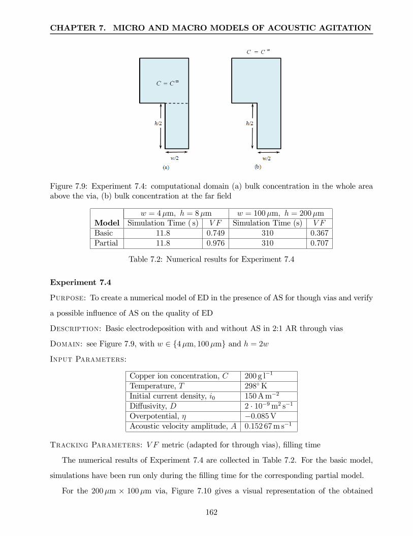
CHAPTER 7. MICRO AND MACRO MODELS OF ACOUSTIC AGITATION
Figure 7.9: Experiment 7.4: computational domain (a) bulk concentration in the whole areaabove the via, (b) bulk concentration at the far field
w = 4µm, h = 8µm w = 100µm, h = 200µmModel Simulation Time ( s) V F Simulation Time (s) V FBasic 11.8 0.749 310 0.367Partial 11.8 0.976 310 0.707
Table 7.2: Numerical results for Experiment 7.4
Experiment 7.4
Purpose: To create a numerical model of ED in the presence of AS for though vias and verify
a possible influence of AS on the quality of ED
Description: Basic electrodeposition with and without AS in 2:1 AR through vias
Domain: see Figure 7.9, with w ∈ 4µm, 100µm and h = 2w
Input Parameters:
Copper ion concentration, C 200 g l−1
Temperature, T 298KInitial current density, i0 150 A m−2
Diffusivity, D 2 · 10−9 m2 s−1
Overpotential, η −0.085 VAcoustic velocity amplitude, A 0.152 67 m s−1
Tracking Parameters: V F metric (adapted for through vias), filling time
The numerical results of Experiment 7.4 are collected in Table 7.2. For the basic model,
simulations have been run only during the filling time for the corresponding partial model.
For the 200µm × 100µm via, Figure 7.10 gives a visual representation of the obtained
162

CHAPTER 7. MICRO AND MACRO MODELS OF ACOUSTIC AGITATION
Figure 7.10: Experiment 7.4, numerical results for the 200µm×100µm through via after 310 sof deposition: (a) and (b) deposition level for the basic and the partial models, respectively;(c) and (d) corresponding ion concentration distributions
results. For the partial model, a high concentration is maintained in the area above the via,
but as the mouth of the via closes, the simulation stops due to a low concentration in the void
area; Figures 7.10(b) and (d). For a basic model, the via is far from being filled during the
same 310 s. On the other hand, due to a faster deposition rate in the case of the partial model,
a considerable crowding effect is observed in the corner regions.
Based on the results of Experiment 7.4, we deduce that, for the through vias Factor 1
improves ion transport and thereby speeds up electrodeposition. Still that does not guarantee
a good quality of filling.
7.5 Micro Model of ED: Study of Factor 2 Impact inTrenches
In this section, we present arguments that show that for trenches Factor 2, i.e., acoustic
streaming inside the via, is unlikely to improve ion transport. Still, megasonic agitation is
helpful for enhancing electrodeposition in blind microvias, due to at least two reasons: (i)
Factor 1 studied in Section 7.4.1 and (ii) resonant bubbles, briefly discussed in this section.
In the case of AS in small trenches, we deal with the model discussed in Section 3.4, with
163

CHAPTER 7. MICRO AND MACRO MODELS OF ACOUSTIC AGITATION
the sound beam filling the via. Mathematically, the first order axial velocity Uax is given by
Rayleigh solution that contains harmonics in both time and space variables. Such a wave
travels inside the via until it hits its bottom, which is essentially a copper cathode. The
incident wave will be superposed by the reflection. Similarly to Section 7.3.2, we can compute
the reflection coeffi cient r by formula (7.2), in which ZP is replaced by the specific acoustic
impedance ZCu of copper. Using copper density and speed of sound in copper, we obtain that
ZCu = 3. 413 8× 10⁷ Pa s m−1, so that
r =34.13 8− 1.5
34.13 8 + 1.5= 0.915 82.
Thus, in the case of electrodeposition of copper, the trench has a highly reflective bottom,
so that more than 90% of energy of the incident wave will be reflected and a standing wave
will be formed, and the ions will not be carried by that wave.
The formation of the standing wave will strongly influence the velocity field in the via.
As far as the second order (streaming) velocity Us is concerned, recall that in the case under
consideration both outer streaming and inner streaming will be observed. The patterns of the
streaming velocity are shown in Figure 3.6, with vortices between nodes and antinodes, which
are only λ/4 apart. This means that in some places motion will be increased, while in other
locations it will be reduced. As Nilson and Griffi ths [115] have put it: “...patterns of acoustic
streaming ... become cellular in character”.
It should not be forgotten that AS, or what we call Factor 2, is not the only effect of mega-
sonic agitation. In the literature, there are multiple pieces of evidence that megasonic agitation
offers a promising approach to enhancing mass transport rates for small vias, including those
of a high aspect ratio. However, we have found no reports that such an improvement takes
place in metal electrodeposition in blind vias due to acoustic streaming.
Whenever examples of positive performance of megasonic agitation are provided, one of
the following happens:
• application is not to electrodeposition, but either to development (see Section 3.6.2) or
cleaning (see Section 3.6.1);
164

CHAPTER 7. MICRO AND MACRO MODELS OF ACOUSTIC AGITATION
• megasonic agitation does provide an improvement, but not necessarily due to acoustic
streaming in a microvia.
For example, Nilson and Griffi ths [115] provide mathematical and numerical models of
development processes in small HAR trenches in the presence of acoustic streaming. They
explicitly insist that their approach is not applicable to ED, since in development the bottom
of a via is made of polymer that is not highly reflective, i.e., there is a rather small impedance
mismatch between that polymer and the liquid. Moreover, in their mathematical models they
completely disregard the reflected wave.
As discussed in Section 3.6.1, megasonic and ultrasonic agitation creates another effect,
different fromAS, known as cavitation, which is formation and collapse of bubbles that generate
so-called microstreaming. The works by Gale and Busnaina [59] as well as by Deymeir and
his colleagues [40, 41, 42, 83] demonstrate that cavitation provides energy to detach undesired
particles from the surface, while AS improves transport of the detached particles away from
the surface. On the other hand, Lamminen et al. [88] point out that in their experiments AS
alone does not have significant effect on cleaning.
In the case of ED combined with megasonic agitation, it is necessarily to separate the
influence of various processes that take place: diffusion controlled ion transport, charge con-
trolled ion transport, acoustic streaming and cavitation. As shown in [73], the dominance of
diffusion controlled ion transport over charge controlled ion transport depends on both ion
concentration in the electrolyte and the frequency of the sound source.
An important study has been carried out by Liu et al. [98]. While admitting that megasonic
agitation may improve the quality of electrodeposition, the authors question whether the
improvement is achieved due to AS. To resolve this issue, they have conducted two series of
experiments of filling HAR microstructures under megasonic agitation. In the first series, no
preprocessing of the electrolyte was done, so that both AS and cavitation affected the quality
of filling. In the second series, the solution was degassed, and that would reduce the chances
of forming cavitation bubbles, so that ED would be affected by AS alone. The experiments
clearly show that the first series have produced filling of a better quality. This implies that
the improvement is mainly achieved due to cavitation, not AS. As stated in [98], cavitation
165

CHAPTER 7. MICRO AND MACRO MODELS OF ACOUSTIC AGITATION
improves ion transport due to microstreaming that occurs near resonant bubbles and also due
to additional buoyancy-driven flows created by these bubbles.
Thus, we conclude that for electrodeposition in blind vias, Factor 2 will not improve ion
transport and there is no need to perform numerical modelling of AS in blind vias. Still, the
arguments given in this section are not fully applicable to through vias. A possible influence
of Factor 2 on ED in through vias is studied in the subsequent sections.
7.6 Micro-Scale Models of Acoustic Streaming inThrough Vias
In order to be able to analyse an impact of AS at the micro level, we need to determine
the distribution of streaming velocity Us inside the via. As follows from Section 7.5, we may
restrict our consideration to through vias only. First, we describe and validate a numerical
approach to computing Us based on the amplitude A delivered by running the macro model
and the so-called driving force that can be prescribed to the elements of the computational
domain. Second, we provide evidence that Us changes insignificantly as the radius of the via
changes. Besides we consider the influence that additional viscous attenuation may have on
Us with respect to the depth of the via.
7.6.1 Modelling of Streaming Velocity in Through Vias
Considering AS in through vias, we deal with a situation of the sound beam filling an open-
end channel. A travelling wave is generated and the channel walls can be seen to satisfy the
non-slip conditions. Such a situation is described in details in Section 3.5.1, where exposition
is based on the works by Nyborg [122] and Frampton et al. [56].
Recall that for the situation under consideration, the driving force F along the channel
walls is split into two components, F (v) that is attributed to viscous effects and a larger force
F (b) that acts in the vicinity of a boundary layer of width δ. These two force components are
responsible for the corresponding components of the streaming velocity Us, with U(b)s taking
large values in the boundary layer and negligible in the remaining part of the channel, where
the component U (v)s dominates. The analytical solutions for the driving force and the AS
166

CHAPTER 7. MICRO AND MACRO MODELS OF ACOUSTIC AGITATION
Figure 7.11: Acoustic streaming velocities in the channel of a radius of 60µm (left half)
velocity are given by (3.26) and (3.27), respectively. Notice in all these formulae the relevant
quantities are expressed in terms of A, the amplitude of the acoustic velocity Ua. As we know
from Section 7.3.2, the value of A is supplied by the corresponding macro model.
Our ultimate goal is to develop an enhanced numerical model of electrodeposition that
includes the streaming effects, and possibly additional flow effects. We are planning to use
PHYSICA to handle these models. Although in principle it is possible to prescribe the AS
velocity field given by the analytical solution in (3.27) directly to the elements of the mesh,
such an approach would prevent us from incorporating further extensions, e.g., to combine ED
with AS and with an additional ordinary flow.
Thus, in order to guarantee suffi cient flexibility of our numerical model, we recommend to
compute the AS velocity numerically, with the driving force given by (3.26) as a flow source
term.
Such an approach needs verification, i.e., demonstration that no accuracy is lost if Us
computed numerically using the driving force, rather than analytically. For a purpose of
verification, the following experiments have been conducted using PHYSICA. We consider a
through via as a channel of a radius of 60µm. Due to symmetry, a half of the channel is taken
as the two-dimensional computational domain with the non-slip wall boundary condition. A
rectangular irregular mesh has been used, with smaller elements in the proximity of the wall;
167

CHAPTER 7. MICRO AND MACRO MODELS OF ACOUSTIC AGITATION
that has been done in order to achieve a higher accuracy of the velocity field in a rather narrow
boundary layer.
Suppose that megasonic agitation is created by a transducer with the parameters
I = 50 kW m−2, f = 1 MHz,
and the macro model supplies the value of amplitude A equal to 0.18 m s−1.
As a result, using (3.14) and (3.23) we obtain
α = 0.0078 m−1, δ = β−1 = 0.6µm.
Each element of the mesh has been associated with the value of Fx computed by (3.26) using
a special subroutine with respect to the element center. As a boundary condition, pressure has
been set to zero at the ends of the channel. Our model uses the flow module of PHYSICA and
numerically solves equation (3.11) to deliver a distribution of the streaming velocity values Us.
The found numerical values have been compared with those computed analytically by
(3.27); see Figure 7.11. It can be seen that the curves that correspond to the numerical AS
velocity found based on the driving force (the blue line) and to the analytically found velocity
(the red line) have the same shape. A good fit is observed with R2 = 0.9897.
7.6.2 Behaviour of Streaming Velocity in Microvias
The approach to computing the AS velocity based on the driving force will become a part of
our combined model of ED in the presence of AS. As we know, during the ED process the
geometry of the channel changes, which poses the question how those changes may affect the
AS velocity.
In a through via, copper is deposited on the walls, thereby reducing the radius r of the
channel.
Figure 7.12 demonstrates that for various radii of the channel the AS velocity Us (i) in the
boundary layer remains the same (all curves are indistiguishable) and (ii) differs insignificantly
in the remaining part of the channel.
When sound travels through a medium, its intensity and amplitude gradually decrease
with the distance. This effect is called attenuation and it is caused by scattering of the sound
168

CHAPTER 7. MICRO AND MACRO MODELS OF ACOUSTIC AGITATION
Figure 7.12: Acoustic streaming velocities for different radii of the channel (left half)
wave and its absorption. Attenuation due to absorption is important when the volume of the
material is large, while attenuation due to scattering has an essential impact either when the
volume is small or in the cases of porous materials. Below, we demonstrate that in microvias
the acoustic streaming velocity Us is subject to insignificant attenuation and can be seen as
independent of the via’s depth.
For a plane wave, let M be a generic variable with amplitude M0, which may correspond
to velocity, pressure, etc. The decrease in amplitude can be expressed using the attenuation
coeffi cient α as
M = M0e−αx,
where x is the direction of the wave propagation.
There are several types of attenuation that can be observed:
1. Viscous attenuation of a one dimensional wave in a free space. The coeffi cient for this
type of attenuation is usually defined in accordance with [115, 122] as
α =1
3δ2(2π/λ)3,
where λ is the wave length and δ is the width of the acoustic boundary layer.
2. When a sound wave travels over a boundary, nonslip boundary conditions are used at
the via’s walls and so-called boundary layer attenuation (also known boundary layer
169

CHAPTER 7. MICRO AND MACRO MODELS OF ACOUSTIC AGITATION
dumping) occurs. In this case, the medium in immediate contact with the surface must
be at rest, but as the distance from the wall increases, layers of medium have a velocity
that increases with the distance as shown in Figure 3.7.
3. Additional viscous attenuation of the amplitude of acoustic pressure Pa or acoustic ve-
locity Ua between the top and the bottom of the via. According to [138], the ratio of the
bottom to the top amplitude is equal to exp(−πhδ/λw), where w and h are the width
and the depth of a via, respectively.
For our purposes, we are interested in additional viscous attenuation. First, we consider its
influence on acoustic velocity Ua, and then discuss attenuation of streaming velocity Us. As
a result, we deduce that the effect of additional viscous attenuation on the streaming velocity
Us can be disregarded.
Figure 7.13: Additional viscous attenuation for frequency of 1 MHz.
For a fixed frequency of agitation of 1 MHz, Figure 7.13 shows amplitude ratios
exp(−πhδ/λw) for various values of via’s width. The vias depth are logarithmically scaled.
It can be seen that for this frequency, attenuation is insignificant for vias with a width
greater than 20µm (top plotted curves) and also for vias of a small depth (less than 10µm).
The plot in Figure 7.14 shows amplitude ratios for vias with the fixed width of 100µm for
different values of frequency.
170

CHAPTER 7. MICRO AND MACRO MODELS OF ACOUSTIC AGITATION
Figure 7.14: Additional viscous attenuation for via’s width 100µm
Attenuation increases at higher frequencies, but still the loss of amplitude is insignificant;
e.g., for f = 1 MHz and an aspect ratio of 10 : 1 the attenuation of amplitude is less than
1.5%.
Table 7.3 shows that for frequency regimes varying from 500 kHz to 2 MHz as the aspect
ratio of the via grows, up to 8 : 1, the amplitude ratio decreases, but insignificantly. Thus, the
additional viscous attenuation for these frequency regimes can be considered AR-independent.
Frequency AR 1:1 AR 8:1 Difference500 kHz 0.999163 0.993324 0.00581 MHz 0.998745 0.990002 0.00872 MHz 0.998327 0.986692 0.0164
Table 7.3: Attenuation values for various frequency regimes
We now pass to the AS velocity Us. Recall that in all formulae presented in Chapter 3,
Us depends on A2, i.e., on the square of the amplitude of Ua. Since for Ua, additional viscous
attenuation is defined as exp(−πhδ/λw), we deduce that for the streaming component of
velocity Us, the ratio between the values at the top and at the bottom of a via will be given
by exp2(−πhδ/λw).
As shown in Figure 7.15, the smallest attenuation of AS speed is observed for w = 100µm
(the top curve). Therefore, for vias of width larger than 100µm attenuation is not essential.
171

CHAPTER 7. MICRO AND MACRO MODELS OF ACOUSTIC AGITATION
Figure 7.15: Attenuation of streaming velocity in vias
The demonstrated characteristics of attenuation in vias are especially important for our
industrial partners, who mainly use a 1 MHz transducer and look at the vias that are 100 −
120µm wide. As shown in this section, for the parameters within these ranges the AS velocity
profile can be considered constant along the via. Thus, in the subsequent sections we can
accurately and effi ciently calculate the ion transport by assuming a constant velocity profile
along the entire depth of a via.
7.7 Micro Models of ED: Study of Factor 2 Impact inThrough Vias
In this section, we analyse whether Factor 2 may have a substantial impact on ion transport
in through vias, and eventually on the quality of ED. For this purpose, we have conducted
numerical experiments with two through vias, identical to those considered in Section 7.4.2
and compare the performance of the full ED model against the partial ED model.
Recall that in the full model, we take into account both Factors 1 and 2. Thus, if we notice
a difference between the performance measures for the full model and the partial model, that
difference can be attributed to Factor 2. On the other hand, if such a difference is insignificant,
we deduce that Factor 2 plays a minor role. As in Section 7.4.2, we use the filling time and
the modified metric V F to judge the quality of filling.
172

CHAPTER 7. MICRO AND MACRO MODELS OF ACOUSTIC AGITATION
A formal description of our experiments is given below.
Experiment 7.5
Purpose: To create a full numerical model of ED for through vias and verify a possible
influence of Factor 2 on the quality of ED
Description: Full and partial ED models for 2:1 AR through vias
Domain: see Figure 7.7, with w ∈ 4µm, 100µm and h = 2w
Input Parameters:
Copper ion concentration, C 80 g l−1 (for w = 4µm); 200 g l−1 (for w = 100µm)Temperature, T 298KInitial current density, i0 150 A m−2
Diffusivity, D 2 · 10−9 m2 s−1
Overpotential, η −0.085 VAcoustic velocity amplitude, A 0.152 67 m s−1
Tracking Parameters: V F metric (adapted for through vias), filling time
Notice that in Experiment 7.5 the value of A has been taken from the output of the macro
model in Experiment 7.2; see Section 7.3.2.
To conduct the experiment for the full model, we have adapted the PHYSICA code for
basic ED, described in Chapter 5. The modified numerical model still calls two PHYSICA
modules: the scalar module and the fluid flow module; however, now the fluid flow module
finds the distribution of the streaming velocity based on the driving force, as described in
Section 7.6.1. The fluid flow module uses the Darcy term given by (5.8).
The numerical results of Experiment 7.5 are collected in Table 7.4, where the data for the
partial model have been found by running Experiment 7.4. The following observations can be
made:
• In both models, the time for filling the vias is the same, i.e., 11.8 s for the 8µm× 4µm
via and 310 s for the 200µm × 100µm via; in all cases the electrodeposition processes
stops due to depletion and a void is formed.
• For the 8µm× 4µm via, the results for both models are virtually indistinguishable.
• For the 200µm× 100µm via, the full model provides a slightly better value of V F than
that achieved in the partial model.
173

CHAPTER 7. MICRO AND MACRO MODELS OF ACOUSTIC AGITATION
w = 4µm, h = 8µm w = 100µm, h = 200µmModel Simulation Time ( s) V F Simulation Time (s) V FPartial 11.8 0.976 310 0.707Full 11.8 0.977 310 0.721
Table 7.4: Numerical results for Experiment 7.5
Having compared the results of Experiment 7.5, we deduce that an impact of Factor 2 can
be seen as insignificant.
Below we give another evidence that Factor 2 indeed has a minor impact. This is done by
comparing the diffusion and convective terms in the concentration equation for through vias
that is derived from (5.3) by replacing the migration term by the convective term, which yields
∂C
∂t= −D∇2C − Us ∇C +RC . (7.3)
Based on the results of Experiment 7.5, we perform an estimation of the diffusion and the
convection terms. For each via we fix a certain time t0 since the beginning of simulation and
then take records of the concentration values along the central vertical cross section of the
via. For the obtained array of data, we use regression to find a polynomial function C(y) that
approximates the concentration distribution along this cross section, where y is the distance
from the geometric centre of the via.
We have taken Us = 6µm s−1, which corresponds to the AS velocity in the middle part of
a via for the given input amplitude A. For the 8µm× 4µm via, our approach is illustrated in
Figure 7.16.
The results of the corresponding computation are shown in Table 7.5. The diffusion and
convective terms are computed by finding the relevant derivatives of the functions C(y); the
diffusion terms being computed for y = 0.
Size of t0 C(y) R2 Diffusion Convectivethe via ( s) (µmolµm−3) term term
8µm× 4µm 4 3 · 10−12y2 + 10−12y + 4 · 10−10 0.9998 1. 2 · 10−8 6 · 10−12
200µm× 100µm 60 6 · 10−14y2 + 10−13y + 7 · 10−10 0.9999 2. 4 · 10−10 6 · 10−13
Table 7.5: Experiment 7.5: comparison convective and diffusion terms
Both found functions C(y) demonstrate a very good fit. It follows that the contribution
of the convective term is much smaller than that of the diffusion term: 2000 times for the
174

CHAPTER 7. MICRO AND MACRO MODELS OF ACOUSTIC AGITATION
Figure 7.16: Experiment 7.5, the 8µm×4µm via: (a) concentration distribution with the cellsalong the vertical centre encircled; (b) the data with the fitted function
8µm× 4µm via and 400 times for the 200µm× 100µm via. Since the convective term reflects
the influence of the AS inside the via, the fact that it is strongly dominated by the diffusion
term explains that the impact of Factor 2 on ion transport inside the via is negligible.
175

Chapter 8
Conclusions and Future Work
In this chapter, we summarise the conclusions that can be derived from the conducted research
and also outline several topics for future research on enhanced electrodeposition and related
areas.
8.1 Conclusions
We list the derived conditions separately for each problem area studied in the thesis, starting
from basic electrodeposition to the enhanced models of electrodeposition.
1. Numerical Modelling of Basic Electrodeposition
(a) A new numerical method (EITM) that allows the explicit tracking the
metal/electrolyte interface has been developed and implemented in PHYSICA; see
Sections 5.3—5.5. The EITM has been validated against real-life measurements (for
ED on a plate, see Experiment 5.1 in Section 5.4) and against known benchmarks
(ED in trenches, see Experiment 5.2 in Section 5.5).
(b) With the aid of the EITM, it has been demonstrated that under the conditions of
basic ED a trench can only be fully filled for fairly low aspect ratios, e.g., 1:2; see
Section 5.6.
(c) The EITM has been the core of a parametric study on the influence of three de-
sign parameters (aspect ratio, bulk ion concentration and initial current density) on
three response parameters (filling time and performance metrics RDT and V F ) for
176

CHAPTER 8. CONCLUSIONS AND FUTURE WORK
a trench with a fixed width; see Experiment 5.3 in Section 5.7. For each response
parameter, a response surface has been determined and the design parameters have
been graded with respect to their influence. For filling time, the most influential
parameter is the initial current density (the higher its value, the shorter the time),
while the other design parameters are of insignificant importance. For RDT and
V F , the aspect ratio is slightly more influential than the other two design parame-
ters, and each of these metrics decreases as the AR increases. Concentration and
current density have almost equal quantitative impact, but the directions of their
influence are opposite: the metric grows as concentration increases and the current
density decreases. Based on the parametric study, an optimisation and prediction
tool has been set up, which allows (i) to find an optimal values of the design para-
meters to achieve a required level of performance, and (ii) to predict the value of a
response parameter for a given choice of values of the design parameters.
(d) The EITM possesses considerable flexibility and allows us to extend the numerical
models of basic ED to their versions enhanced by acoustic streaming and/or ordinary
flow; see Experiment 7.5 in Section 7.7.
(e) The main conclusion derived from all conducted numerical experiments that the
conditions of basic ED normally do not provide good quality via filling, due to a
premature closure of the mouth of the via and formation of a void. The main reason
of this underperformance is insuffi cient ion transport, and enhancement is required
in order to improve the ion supply into vias.
2. Ordinary Flow in a Plating Cell
(a) A general methodology which links the flow phenomena that affect ion transport
at the macro level and the micro level in a plating cell has been developed; see
Section 6.2. The methodology not only captures the interaction between the macro
and micro models, but also allows to deduce recommendations on the design of a
plating cell with a purpose of improving ion transport.
(b) At the macro level, the developed numerical models allow us to find distributions
177

CHAPTER 8. CONCLUSIONS AND FUTURE WORK
of pressure, velocity and ion concentration in any part of the plating cell, including
the surfaces of the panels, which serve as input for the relevant micro models.
Statistically justified conclusions regarding performance for various cell designs have
been drawn. In particular, it has been demonstrated that to achieve a more uniform
distribution of pressure and velocities on the surfaces of the two panels inserted into
the cell, the inlet has to be moved from the corner of the cell (Design 1) to the middle
of the side of the cell (Design 2). See Sections 6.3 and 6.4.
(c) Experiments with numerical micro models in Section 6.5 demonstrate that ei-
ther tangential or direct flow improves the ion transport more significantly for the
straight trenches rather than for the tapered trenches of the same aspect ratio.
(d) Experiments with numerical micro models in Section 6.6 demonstrate that a bet-
ter ion transport in through vias under tangential flow is achieved due to a large
pressure/velocity drop at the sides of the board. This generates a recommendation
on a possible cell design, e.g., regarding the location of the inlet or its flow rate
characteristics.
(e) The parametric study in Section 6.7 regarding the direct flow in tapered trenches
with a fixed diameter of the top mouth supports a conclusion that ion transport in
the straight trenches overperforms that in the tapered trenches.
(f) Conclusions in Items 2(c) and 2(e) above do not contradict the real-life observations
that the quality of filling for tapered trenches is better than for the straight trenches
of the same aspect ratio. A better quality of ED that is observed in practice for
the tapered trenches should be attributed to factors other than ion transport by a
forced flow, most likely to the reduction in the volume of deposition. This issue still
needs further, more systematic studies.
3. Numerical Modelling of Acoustically Induced Flows
(a) A general methodology which links the phenomena that are induced by megasonic
agitation and affect ion transport at the macro level and the micro level in a plating
cell has been developed; see Section 7.2. As in the case of the ordinary flow, the
178

CHAPTER 8. CONCLUSIONS AND FUTURE WORK
methodology links the macro and micro models, and supplies redesign recommen-
dations of a plating cell, e.g., possible changes to a position and acoustic parameters
of the transducer.
(b) At the macro level, the first and the second order acoustic phenomena induced by
megasonic agitation have been started separately.
i. The second order phenomena, i.e., acoustic streaming in the cell, have been
modelled based on the driving force for the travelling wave in an open space;
see Section 7.3.1. For the model that combines AS and ordinary flow, it has been
observed that for the used parameters AS is more powerful, and thereby con-
tributes more considerably to improving the mixing in the bath and eventually
ion transport. Besides, AS generates a thin boundary layer along the surfaces
of the panels. This justifies the fact that in the micro model a high level of
bulk ion concentration can be maintained immediately above the mouth of a
microstructure; in our study we call this Factor 1 and it is taken into account
in micro models of enhanced ED.
ii. The numerical macro models with the first order phenomena, i.e., the harmonic
component of the acoustic wave, output the amplitude of the acoustic velocity
on the surface of a panel; see Section 7.3.2. This amplitude acts as part of the
input for the micro model for computing the AS velocity inside the via, which
we call Factor 2 in our study of micro models of enhanced ED.
(c) For the micro models in through vias, a method for computing the AS velocity
distribution has been developed based on
• the acoustic velocity amplitude supplied by the macro model;
• analytical solution for the streaming driving force in narrow open channels by
Frampton et al. [56];
• our study that shows that amplitude attenuation along the depth of the via
can be ignored.
See Section 7.6.
179

CHAPTER 8. CONCLUSIONS AND FUTURE WORK
4. Numerical Modelling of Electrodeposition Enhanced by Acoustic Streaming
(a) Numerical experiments aimed at comparing basic ED models with partial ED mod-
els that take into account Factor 1 (see Item 3(b)i above) have been conducted. For
the latter model, a modified boundary condition assumes the same bulk concen-
tration in the whole area above the mouth of the via, rather than at the far field.
We deduce that for partial models a higher deposition rate is observed for both
blind and through vias. The same vias under the conditions of the partial model
appear to be more filled than under the conditions of basic ED; for smaller trenches
a complete filling has been achieved. Still, overall quality of filling for the partial
models is dubious, with a considerable crowding effect at the mouth.
(b) For trenches, acoustic streaming, i.e., Factor 2 (see Item 3(b)ii above) has no major
influence, which follows from both theoretical considerations regarding AS in narrow
closed channels with a reflective bottom and real-life experiments, e.g., by Liu et
al. [98]; see Section 7.5.
(c) For through vias Factor 2 has no major influence either. This is demonstrated by
the numerical experiments with a partial model and the full model, the latter model
additionally takes into account Factor 2. For implementation of the full model, an
appropriate adaptation of the EITM has been done. It has also been demonstrated
that the concentration flux due to AS is several orders smaller than that due to
diffusion.
(d) Thus, we deduce that AS in small vias cannot be seen as an enhancing factor. This
does not mean that megasonic agitation has no positive influence. For example, AS
at the macro level improves the mixing in the plating cell, see Item 3(b)i above.
Besides, there are other phenomena that accompany megasonic agitation, e.g., reso-
nant bubbles and thermal effects. These phenomena are not a subject of this study
and require further research.
180

CHAPTER 8. CONCLUSIONS AND FUTURE WORK
8.2 Future Work
In this section, we outline several directions of possible future work that follow from this thesis.
• In this thesis, the EITM has been applied to straight trenches and straight through
vias. In its current form, the EITM uses a regular rectangular mesh, with identical
elements inside the microvia. To make the method applicable for handling tapered vias
the modification is required that would involve other than rectangular mesh elements.
• The EITM has been proved to be a useful tool that allows us not only to handle numerical
models of basic ED, but also their extensions, such as models that combine ED with AS.
Including AS into a numerical model requires a very accurate computation of velocity for
the elements of the boundary layer. The thickness of the boundary layer is very small,
e.g., less than 0.6µm for megasonic agitation with frequency of 1 MHz. For accurate
definition of the boundary layer, it has to be at least several cells thick, which causes a
problem, especially for vias of 100µm or wider, since with the growth of the elements
a simulation run becomes time consuming. An interesting research topic is to develop
an implementation of the EITM that allows a finer mesh cells in the vicinity of the
copper/electrolyte interface, with dynamic remeshing to reflect the moving interface.
• The EITM has been developed under the assumption that overpotential remains constant
during the simulation, see Section 5.2. To improve the accuracy of the model, the changes
of overpotential in each time step should be taken into account.
• Using additives is the most common way of controlling electrodeposition rate in mi-
crovias. The approaches to numerical modelling of ED in the presence of additives are
described in Section 5.1. It is an attractive goal to modify the EITM in order to study
the impact of additives on the quality of ED.
• In order to further understand better the role of ordinary flow in enhancing ED, it is
an interesting research goal to experiment with the numerical models that integrate ED
and ordinary flow at the micro level. A combined model of this type can be designed
similarly to the models that combine ED and AS, see Section 7.7.
181

CHAPTER 8. CONCLUSIONS AND FUTURE WORK
• Many practitioners report that higher quality of ED is achieved for tapered trenches,
as compared to straight trenches of the same aspect ratio. We think this is due to
smaller volume of the tapered trench. Besides, due to its shape the bottom-up filling
may naturally occur, leading to a superconformal filling. A separate additional study of
all aspects of ED in tapered trenches is required.
• In this work, the numerical models that combine AS and ordinary flow in a plating cell
has been studied in 2D only. It is desirable to extend these models to 3D.
• We have demonstrated that deposition rates increase if bulk concentration is maintained
high due to megasonic agitation; see Section 7.4 on the impact of Factor 1. Further study
is required on the overall filling quality under these conditions.
• We have identified one aspect of megasonic agitation, namely Factor 1, that considerably
affects ion transport in microvias. It will be interesting to determine the influence of other
phenomena that accompany megasonic agitation (e.g., resonant bubbles, thermal effect)
on ion transport and quality of ED.
• Further testing and validation of numerical simulation results against real-life experi-
mental measurements is to be performed.
182

Index
acoustic boundary layer, 29
Acoustic streaming, 28
continuity equation, 32
driving force, 35
Eckart type, 29
equation of motion, 32
Quartz Wind, 29
Rayleigh type, 30
Schlichting type, 30
Additive, 26
accelerator, 26
inhibitor, 26
leveler, 26
suppressor, 26
anode, 14
Aspect ratio (AR), 1
high (HAR), 21
Attenuation, 168
Additional viscous, 170
boundary layer, 169
coeffi cient, 169
viscous, 169
cathode, 14
Computational
electromagnetics, 57
fluid dynamics, 57, 107
modelling, 57
solid mechanics, 57
control volume, 59
current density, 19
Current distribution
primary, 19
secondary, 19
tertiary, 20
diffusion, 17
diffusive material flux, 18
diffusivity, 17
discretisation, 58
Einstein relation, 18
Electrodeposition, 14
basic, 24
conformal, 22
enhanced, 27
LIGA, 13
performance metrics
dimple depth, 23
relative deposition thickness, 23
via fill, 23
183

INDEX
subconformal, 22
superconformal , 22
electrolyte, 16
Equation
Butler-Volmer, 20
continuity, 58
general transport, 58
Laplace, 77
mass conservation, 105
momentum conservation, 105
Nerst-Planck, 18
Flow
Darcy term, 83
hydrodynamic boundary layer, 106
inlet, 106
laminar, 105
outlet, 106
residence time, 107
turbulent, 105
integrated circuit, 10
interface, 86
ionic mobility, 18
Law
Faraday, 19
Ohm, 19
mass flux, 18
Mesh
structured, 58
unstructured, 59
meshing, 58
Method
Explicit Interface Tracking (EITM), 81
Fast Marching (FMM), 71
Finite Difference (FDM), 59
Finite Element (FEM), 59
Finite Volume (FVM), 59
Level Set (LSM), 71
Monte Carlo, 74
Particle Image Velocimetry (PIV), 127
successive approximations, 33
microelectronics, 9
migration, 17
Model
macro-scale, 108, 148
micro-scale, 109, 148
multi-physics, 58
overpotential, 19
printed circuit board (PCB), 1
Reynolds number, 29, 105
scaling, 80
sink, 77
Software
COMSOL Multiphysics, 63
PHOENICS, 62
PHYSICA, 61
VisualDOC, 65
184

INDEX
Design of Experiments (DoE), 65
Response Surface (RS) optimisation, 66
sound reflection coeffi cient, 155
specific acoustic impedance, 154
Tafel slope, 20
Theorem
divergence, 60
Gauss-Ostrgradsky, 60
time averaging, 35
Trench, 11
straight, 124
tapered, 124
Via, 11
blind, 11
buried, 11
open, 11
through, 11
185

Bibliography
[1] Aanonsen S.I., Barkve T., Tjotta J.N. and Tjotta S. Distortion and harmonic genera-
tion in the nearfield of a finite amplitude sound beam. Journal of Acoustical Society of
America, 1984: 75(3), 749—768.
[2] Adalsteinsson D., Sethian J. A fast level set method for propagating interfaces. Journal
of Computational Physics, 1995: 118, 269—277.
[3] Adalsteinsson D., Sethian J. A level set approach to unified model for etching, deposition,
and lithography, I: Algorithms and two-dimentional simulations. Journal of Computa-
tional Physics, 1995: 120, 128—144.
[4] Adalsteinsson D., Sethian J. A level set approach to unified model for etching, deposition,
and lithography, II: Tree-dimensional simulations. Journal of Computational Physics,
1995: 122, 348—366.
[5] Adalsteinsson D., Sethian J. A level set approach to unified model for etching, depo-
sition, and lithography, III: Redeposition, Reemission, surface diffusion, and complex
simulations. Journal of Computational Physics, 1997: 138, 193—223.
[6] Aktas M.K. and Farouk B. Numerical simulations of acoustic streaming generated by
finite-amplitude resonant oscillations in an enclosure. Journal of Acoustical Society of
America, 2004: 116(5), 2822—2831.
[7] Andres J.M. and Ingard U. Acoustic streaming at high Reynolds numbers. Journal of
Acoustical Society of America, 1953: 25(5), 928—932.
186

BIBLIOGRAPHY
[8] Andres J.M. and Ingard U. Acoustic streaming at low Reynolds numbers. Journal of
Acoustical Society of America, 1953: 25(5), 932—938.
[9] Andricacos P.C., Uzoh C., Dukovic J.O., Horkans J. and Deligianni H. Damascene copper
electroplating for chip interconnects. IBM Journal of Research and Development, 1998:
42(5), 567—574.
[10] Bakhtari K., Guldiken R.O., Makaram P., Busnaina A.A. and Park J.-G. Experimental
and numerical investgation of nanoparticle removal using acoustic streaming and the
effect of time. Journal of the Electrochemical Society, 2006: 153 (9), G846—G850.
[11] Bailliet H., Gusev V., Raspet R. and Hiller R.A. Acoustic streaming in closed thermoa-
coustic devices.. Journal of Acoustical Society of America, 2001: 110(4), 1808—1821.
[12] Bathe K.J. Finite Element Procedures, Prentice-Hall: New York, 1996.
[13] Beica R., Sharbono C. and Ritzdorf T. Through Silicon Via Copper Electrodeposition
for 3D Integration. The 58-th Electronic Components and Technology Conference, 2008,
577-583.
[14] Black K. Business Statistics. An Introductory Course. West Publishing Company: St
Paul, 1992.
[15] Boluriaan S. and Morris P.J. Acoustic streaming: from Rayleigh to today. International
Journal of Aeroacoustics, 2003: 2(3/4), 255—292.
[16] Boovaragaran V. and Basha C.A. A novel approach for computing tertiary current dis-
tributions based on simplifying assumptions. Journal of Applied Electrochemistry, 2006:
36, 745—757.
[17] Bossart R., Joly N. and Bruneau M. Hybrid numerical and analytical solutions for
acoustic boundary problems in thermo-viscous fluids. Journal of Sound and Vibration.
2003: 263, 69—84.
187

BIBLIOGRAPHY
[18] Brereton G.J. and Bruno B.A. Partical removal by focused ultrasound. Journal of Soud
and Vibration. 1994: 173(5), 683—698.
[19] Buoni M. and Petzold L. A effi cient, scalable numerical algorothm for the simulation of
electrochemical systems on irregular domains. Journal of Computational Physics, 2007:
225, 2320—2332.
[20] Buoni M. and Petzold L.A. An algorithm for simulation of electrochemical systems with
surface-bulk coupling strategies. Journal of Computational Physics, 2010: 229, 379—398.
[21] Busnaina A.A. and Gale G.W. Removal of silica particles from silicon substrates using
megasonic cleaning. Particulate Science and Technology, 1997: 15, 361—369.
[22] Busnaina A.A. and Elsawy T.M. Post-CMP cleaning using acoustic streaming. Journal
of Electronic Materials, 1998: 127(10), 1095—1098.
[23] Byrne P., Bosander P., Parhammar O. and Fontes E. A primary, secondary and pseudo-
tertiary mathematical modal of a chlor-alkali membrane cell. Journal of Applied Elec-
trochemistry, 2000: 30, 1361—1367.
[24] Chan S.H. and Chen H.Y. Modelling of through-hole electrodeposition. Part I: Effect of
electrical migration. Journal of Applied Electrochemistry, 2001: 31, 605—616.
[25] Chan S.H. and Chen H.Y. Modelling of through-hole electrodeposition. Part II: Experi-
mental study. Journal of Applied Electrochemistry, 2001: 31, 617—622.
[26] Chan S.H. and Chen H.Y. The current distribution in through-hole electrodeposition. I:
Mass stransfer. Chemical Engineering Communications, 2004: 191, 861—880.
[27] Chivilikhin S., Landau U. and Malyshev E. Current distribution on a resistive wafer un-
der copper deposition kinetics. Proceedings of the AIChE Annual Meeting, SanFrancisco,
CA, 2003: Paper 190b, Section TK.
[28] COMSOL Multiphysics Modelling Guide, AB Comsol - Comsol Ltd, 2006.
188

BIBLIOGRAPHY
[29] Cooper P.I., Sheridan J.C. and Flood G.J. The effect of sound on forced convection over
a flat plate. International Journal of Heat and Fluid Flow, 1986: 7, 61—68.
[30] Cosgrove J.A., Buick J.M., Pye S.D. and Greated C.A. PIV applied to Eckart streaming
produced by a medical ultrasound transducer, Ultrasonics, 2001: 39, 461—464.
[31] Costello S., Flynn D., Kay R.W., Desmulliez M.P.Y., Strusevich N., Patel M.K., Bai-
ley C., Jones A.C., Bennet M., Price D., Habeshaw R., Demore C. and Cochran S. Elec-
trodeposition of copper into PCB vias under megasonic agitation, Proceedings of 22nd
Micromechanics and Microsystems Technology Europe Workshop, MME 2011, Toens-
berg, Norway, 2011.
[32] Costello S., Strusevich N., Patel M.K., Bailey C., Flynn D., Kay R.W., Price D., Ben-
nett M., Jone A.C., Habeshaw R., Demore C., Cochran S. and Desmulliez M.P.Y. Char-
acterisation of ion transportation during electroplating of high aspect ratio microvias
using megasonic agitation. Proceedings of EMPC-2011 - 18th European Microelectronics
and Packaging Conference, Brighton, 2011, pp. 233—239.
[33] Costello S., Strusevich N., Flynn D., Kay R.W., Patel M.K., Bailey C., Price D., Ben-
net M., Jones A.C. and Desmulliez M.P.Y. Electrodeposition of copper into high aspect
ratio PCB micro-via using megasonic agitation. Proceedings of DTIP 2012, Symposium
on Design, Test, Integration & Packaging of MEMS/MOEMS, Cannes, France, 2012.
[34] Costello S., Strusevich N., Flynn D., Kay R.W., Patel M.K., Bailey C., Price D., Bennet
M., Jones A.C. and Desmulliez M.P.Y. Electrodeposition of copper into PCB vias using
megasonic agitation, Microsistem Technologies, 2012, In Press, doi: 10.1007/s00542-013-
1746-7.
[35] Croft N., Pericleous K. and Cross M. Physica: A multiphysics enviroment for complex
flow processes. Numerical Methods in Laminar and Turbulent Flow, 1995: 9 (Part 2),
1269-1280.
[36] Cross M., Chow P., Bailey C., Croft N., Eweer J., Leggett P., McManus K., Pericleous K.
and Patel M. PHYSICA — a software environment for the modeling of multi-physics
189

BIBLIOGRAPHY
phenomena, ZAMM - Journal of Applied Mathematics and Mechanics, 1996: 76, 105-
108.
[37] Currie I.G. Fundamental Mechanics of Fluid, 3d edition, M. Dekker: New York, 2003.
[38] Delany M.E., Bazley E.N. Acoustical properties of fibrous absorbent materials. Applied
Acoustics, 1970: 3, 105—116.
[39] Devcic-Kuhar B., Pfaffenberger S., Groschl M., Kollmann K., Benes E. and Gottsauner-
Wolf M. In vitro thrombolysis enhanced by standing and travelling ulrtasound wave
fields. Ulstasound in Medicine and Biology, 2002: 28(9), 1181—1187.
[40] Deymier P.A., Khelif A., Djafari-Rouhani B., Vasseur J.O. and Raghavan S. Theoretical
calculation of the acoustic force on a patterned silicon wafer during megasonic cleaning.
Journal of Applied Physics, 2000, 88: 2423—2429.
[41] Deymier P.A., Vasseur J.O., Khelif A. Second-order sound field during megasonic clean-
ing of patterned silicon wafers: Application to ridges and trenches. Journal of Applied
Physics, 2001: 90, 4211—4218.
[42] Deymier P.A., Vasseur J.O., Khelif A.,Djafari-Rouhani B., Dobrzynski L. and Ragha-
van S. Streaming and removal forces due to second-order sound field during megasonic
cleaning of silicon wafers. Journal of Applied Physics, 2000: 88, 6821—6835.
[43] Douglas J.F., Gasiorek J.M. and Swaffi eld J.A. Fluid Mechanics, 3rd Edition, Longman
Group Ltd: Larlow, UK, 1995, pp. 339—346.
[44] Drews T.O, Webb E.G., Ma D.L., Alameda J., Braatz R.D. and Alkire R.C. Coupled
mesoscale—continuum simulations of copper electrodeposition in a trench. Materials, In-
terfaces, and Electrochemical Phenomena, 2004: 50(1), 226—240.
[45] Dukovic J.O. Computation of current distribution in electrodeposition, a review. IBM
Journal of Research and development, 1990: 34(5), 693—705.
190

BIBLIOGRAPHY
[46] Eckart K. Vortices and streams caused by sound waves. Physical Review, 1948: 73(4),
68—76.
[47] Engelbrecht H. and Pretorius L. The effect of sound on natural convection from a vertical
flat plate. Journal of Sound and Vibration, 1992: 158(2), 213—218.
[48] Ehlers K.M and Koiller J., Could cell membranes produce acoustic streaming? Making
the case for synechocossus self-propulsion. Mathematical and Computer Modelling, 2011:
53(7-8), 1489—1504.
[49] Fallah N.A, Bailey C., Cross M. and Taylor G.A. Comparison of finite element and
finite volume methods application in geometrically nonlinear stress analysis. Applied
Mathematical Modelling, 2000, 24, 439-455.
[50] Fang C. Croissance electrolytique du cuivre appliquee a la technologie System in Package,
PhD Thesis, University of Rennes, France, 2011.
[51] Fang C., Le Corre A. and Yon D. Copper electroplating into deep microvias for the “SiP”
application, Microelectronic Engineering, 2011: 88, 749—753.
[52] Fedorov A.Y. and Tsoi P.I. Acoustic streaming in a boundary layer. Journal of Ap-
plied Mechanics and Technical Physics, 1978: 19(3), 348—351 Translated from Zhurnal
Prikladnoi Mekhaniki i Tekhnicheskoi Fiziki. 1978: 3, 84—87.
[53] FEMGV, Femsys Ltd, http://www.femsys.co.uk.
[54] Ferziger J.H. and Reric M. Computational Methods for Fluid Dynamics, Springer—Verlag
Berlin Heidelberg, Germany, 1996.
[55] Frenkel V., Gurka R., Liberzon A., Shavitt U. and Kimmel E. Preliminary investigations
of ultrasound induced acoustic streaming using particle image velocimetry. Ultrasound,
2001: 39, 153—156.
[56] Frampton K.D., Martin S.E. and Minor K. The scaling of acoustic streaming for appli-
cation in micro-fluidic devices. Applied Acoustics, 2003: 64, 681—692.
191

BIBLIOGRAPHY
[57] Frampton K.D., Minor K. and Martin Sh. Acoustic streaming in micro-scale cylindrical
channels. Applied Acoustics, 2004: 65, 1121—1129.
[58] Frommelt T., Gogel D., Kostur M., Talkner P., Hanggi P. and Wixforth A. Flow patterns
and transport in Rayleigh surface acoustic wave streaming: combined finite element
method and raytracing numerics versus experiments. IEEE Transactions on Ultrasonics,
Ferroelectrics, and Frequency Control, 2008: 55(10), 2298—2305.
[59] Gale G.W and Busnaina A.A. Roles of cavitation and acoustic streaming in megasonic
cleaning. Particulate Science and Technology, 1999: 17, 229—238.
[60] Gamburg Y.D. and Zangari G. Theory and Practice of Metal Electrodeposition, Springer:
Berlin, 2011.
[61] Georgiadou M., Veyret D., Sani R.L. and Alkire R.C. Simulation of shape evolution dur-
ing electrodeposition of copper in the presence of additive. Journal of the Electrochemical
Society, 2001: 148 (1), C54—C58.
[62] Georgiadou M. Modeling current density distribution in electrochemical systems. Elec-
trochimica Acta, 2003: 48, 4089—4095.
[63] Goldbach S., Van Den Bossche B., Daenen T., Deconinck J and Lapicque F. Copper
deposition on micropatterned electrodes from an industrial asid copper plating bath.
Journal of Applied Electrochemistry, 2000: 30, 1—12.
[64] Griffi ths S.K., Nilson R.H., Ting A., Bradshaw R.W., Bonivert W.D. and Hruby J.M.
Modeling electrodeposition for LIGA micridevice fabrication. Microsystem Technologies,
1998: 4, 98—101.
[65] Haghdoost A., Pitchumani R. Numerical Analysis of electrodeposition in microcavities.
Electrochimica Acta, 2011: 56, 8260—8271.
[66] Hamilton M.F., Ilinskii Y.A. and Zabolotskaya E.A. Acoustic streaming generated by
standing waves in two-dimensional channels of arbitrary width. Journal of Acoustical
Society of America, 2003: 113(1), 153—160.
192

BIBLIOGRAPHY
[67] Hamilton M.F., Ilinskii Y.A. and Zabolotskaya E.A. Thermal effects on acoustic stream-
ing in standing waves. Journal of Acoustical Society of America, 2003: 114(6), 3092—3101.
[68] Hariharan P., Myers M.R., Robinson R.A., Maruvada S.H., Sliwa J. and Banerjee R.K.
Characterization of high intensity focused ultrasound transducers using acoustic stream-
ing. Journal of Acoustical Society of America, 2008: 123(3), 1706—1719.
[69] Haydock D. and Yeomans J.M. Acoustic enhancement of diffusion in porous material.
Ultrasonics, 2003: 41, 531—538.
[70] Hughes M., Bailey C., McManus K. Multi physics modelling of the electrodeposition
process. Proceedings of EuroSimE 2007, 2007, London, UK, 206—213.
[71] Hughes M.,Strussevitch N., Bailey C., McManus K., Kaufmann J., Flynn D. and Desmul-
liez M. Numerical algorithms for modelling electrodeposition: Tracking the deposition
front under forced convection from megasonic agitation. International Journal for Nu-
merical Methods in Fluids, 2010: 64(3), 237—268.
[72] Hyun S., Lee D.R. and Loh B.G. Investigation of convective heat transfer augmentation
using acoustic streaming generated by ultrasonic vibrations. International Journal of
Heat and Mass Transfer, 2005: 47, 703—718.
[73] Hyde M.E.and Compton R.G. How ultrasound influences the electrodeposition of metals.
Journal of Electroanalytical Chemistry, 2002: 531, 19—24.
[74] Jang J.-G., Lim S.-K., Kim T.-Y., Kim N.-J. and Su S.-J. Fabrication and characteristics
of through silicin vias interconnection by electroplating. Japanese Journal of Applied
Physics, 2011: 50, 01BG07-1—01BG07-4.
[75] Jonson P., Sahlstrand-Jonson P., Holmer N.G., Persson H.W., Jannert M. and Jansson
T. Feasibility of measuring acoustic streaming for improved diagnosis of rhinosinisitis.
Ulstasound in Medicine and Biology, 2008: 34(2), 228—238.
193

BIBLIOGRAPHY
[76] Josell D., Baker B., Witt C., Wheeler D. and Moffat T.P. Via filling by electrodeposition.
Supeconformal silver and copper and conformal nickel. Journal of the Electrochemical
Society, 2002: 149(12), C637—C641.
[77] Josell D., Moffat T.P. andWheeler D. Superfilling when absorbes accelerators are mobile.
Journal of the Electrochemical Society, 2007: 154(4), D208—D214.
[78] Josell D., Wheeler D., Huber W.H., Bonevich J.E. and Moffat T.P. A simple equation
for predicting superconformal electrodeposition insubmicrometer trenches. Journal of the
Electrochemical Society, 2001: 148(12), C767—C773.
[79] Josell D., Wheeler D. and Moffat T.P. Gold superfill in submicrometers trenches: exper-
iment and prediction. Journal of the Electrochemical Society, 2006: 153(1), C11—C18.
[80] Kamakura T., Sudo T., Matsuda K. and Kumamoto Y. Time evolution of acoustic
streaming from a planar ultrasound souce. Journal of Acoustical Society of America,
1996: 100(1), 132—138.
[81] Kaufmann J., Desmulliez M., Price D., Hughes M., Strusevich N. and Bailey C. Influence
of Megasonic Agitation on the Electrodeposition of High Aspect Ratio Blind Vias. 2nd
Electronics Systemintegration Technology Conference, Greenwich, UK, 2008, 1235—1239.
[82] Kaufmann J.G., Desmulliez M.P.Y., Tian Y., Price D., Hughes M., Strusevich N., Bailey
C., Liu C. and Hutt D. Megasonic Agitation for enhanced electrodeposition of copper.
Microsystem Technologies, 2009: 15, 1234—1254.
[83] Keswani M., Raghavan S. and Deymier P. Study of bubble activity in a megasonic field
using an electrochemical technique. IEEE Transactions on Semiconductor Manufactur-
ing, 2011, 24, 513—518.
[84] Kirby B.J. Micro- and Nanoscale Fluid Mechanics: Transport in Microfluidic Devices.
Cambridge University Press, Cambridge et al., 2010.
[85] Kondo K., Yonezawa T., Mikami D., Okudo T., Taguchi Y., Takahashi K. and Barkey
D.P. High-aspect-ratio copper-via-filling for three-dimensional chip stacking, II. Reduced
194

BIBLIOGRAPHY
electrodeposition process time. Journal of the Electrochemical Society, 2005: 152(11),
H173-H177.
[86] Kondo K., Nakamura T. and Okamoto N. Correlation between Cu (I)-complex and filling
of via cross sections by copper electrodeposition. Journal of Applied Electrochemistry,
2009: 39, 1789—1795.
[87] Lam C.H., Kooij B.J. and De Hoop A.T. Impulsive sound reflection from an absorptive
and dispersive planar boundary. Journal of Acoustical Society of America, 2004: 116(2),
677—685.
[88] Lamminen M.O., Walker H.W. andWeavers L.K. Mechanisms and factors influencing the
ultrasonic cleaning of particle-fouled ceramic membranes. Journal of Membrane Science,
2004, 237, 213—223.
[89] Landau U., Malyshev E., Akolkar R. and Chivilikhin S. Simulations of ’bottom-up’
fill in via plating semiconductor interconnects. AIChE Annual Meeting, SanFrancisco,
California, 2003: Paper 189d, Section TK.
[90] Lasance C.J.M. and Aarts R.M. Synthetic Jet Cooling Part I: Overwiew of heat transfer
and acoustics. 24th IEEE SEMI-THERM Symposium, 2008, 20—25.
[91] Lee C.P. and Wang T.G. Outer acoustic streaming. Journal of Acoustical Society of
America, 1990: 88(5), 2367—2375.
[92] Lefebvre M., Allardyce G., Scita M., Tsuchida H., Kusaka M. and Hayachi S. Copper
electroplativg technology for Microvia Filling. Circuit World, 2003: 29(2), 9—14.
[93] Lefebvre M., Najjar E., Gomez L. and Barstad L. Electroplating for HDI and packaging
substrates, Part 1. Printed Circuit Design & Fab, 2009, August.
[94] Lei H., Henry D. and BenHalis H. Numerical study of the influence of a longitudinal
sound field on natural convection in cavity. International Journal of Heat and Mass
Transfer, 2006: 49, 3601—3616.
195

BIBLIOGRAPHY
[95] Li X., Drews T.O., Rusli E., Xue F., He Y., Braatz and Alkire R. Effect of additives
on shape evolution during electrodeposition: I. Multiscale simulation with dynamically
coupled Kinetic Monte Carlo and Moving-Boundary finite-volume codes. Journal of the
Electrochemical Society, 2007: 154(4), D230—D240.
[96] Lighthill J. Acoustic streaming. Journal of Sound and Vibration, 1978: 61(3), 391—418.
[97] Lin H., Busnaina A.A. and Suni I.I. Invetigation of ionic contamination removal from
silicon dioxide surfaces. Surface Ingineering, 2002: 18(3), 1—4.
[98] Liu G., Huang X., Xiong Y. and Tian Y. Fabrication HARMS by using megasonic assisted
electoforming. Micorsystem Technologies, 2008: 14, 1223—1226.
[99] Liu S. and LiuY. Modeling and Simulation for Microelectronic Packaging Assembly:
Manufacturing, Reliability and Testing, Wiley, 2011.
[100] Loh B.G., Hyun S., Ro P.I. and Kleinstreuer C. Acoustic streaming induced by ultrasonic
flexural vibrations and associated enhancement of convective heat transfer. Journal of
Acoustical Society of America, 2002: 111(2), 875—883.
[101] Low C.T.J., Roberts E.P.L. and Walsh F.C. Numerical simulation of the current, po-
tential and concentration distributions along the cathode of a rotating cylinder hull cell.
Electrochimica Acta, 2007: 52, 3831—3840.
[102] Lühn O., Van Hoof C., Ruythooren W. and Celis J.-P. Filling of microvia with an aspect
ratio of 5 by copper electrodeposition. Electrochemica Acta, 2009: 54, 2504—2508.
[103] Malyshev E., Landau U. and Chivilikhin S. Modeling the deposit thickness distribution
in copper electroplating of semiconductor wafer interconnects. Proceedings of the AIChE
Annual Meeting, SanFrancisco, CA, 2003: Paper 190c, Section TK.
[104] Mattsson E. and Bockris J, Galvanostatic studies of the kinetics of deposition and dis-
solution in the copper + copper sulphate system. Transactionf of the Faraday Society,
1959: 55, 1586—1601.
196

BIBLIOGRAPHY
[105] Merchant S.M., Kang S.H., Sanganeria M., van Schravendijk B. andMountsier T. Copper
interconnects for semiconductor devices. Journal of the Minerals, Metals and Materials
Society, 2001: 53, 43-48.
[106] Mitome H. The mechanism of generation of acoustic streaming. Electronics and Com-
munications in Japan, 1998: Part 3, 81(10), 1—8.
[107] Moffat T.P., Baker B., Wheeler D., Bonevich J.E., Edelstein M., Kelly D.R., Gan L.,
Stafford G.R., Chen P.J., EgelhoffW.F. and Josell D. Superconformal Electrodeposition
of Silver in Submicrometer Features. Journal of the Electrochemical Society, 2002: 149(8),
C423—C428.
[108] Moffat T.P., Wheeler D. and Josell D. Electrodeposition of copper in the SPS_PEG_Cl
additive system. Journal of the Electrochemical Society, 2004: 151(4), C262—C271.
[109] Moffat T.P., Wheeler D., Kim S.-K. and Josell D. Curvature enhanced adsorbate coverage
model for electrodeposition. Journal of the Electrochemical Society, 2006: 153(2), C127—
C132.
[110] Murata Y., Kimura S., Takei S., Minagawa K., Takimoto J. and Koyama K. Generation
of an enhanced acoustic streaming in a bounded space. Journal of Acoustical Society of
America, 1997: 102(5), 2536—2538.
[111] Myers M.R., Hariharan P. and Banerjee R.K. Direct methods for characterizing high-
intensity focused ultrasound transducers using acoustic streaming. Journal of Acoustical
Society of America, 2008: 124(3), 1790—1802.
[112] Nabavi M., Siddiqui K. and Dargahi J. Experimental investigation of the formation
of acoustic streaming in a rectangular enclosure using a synchronized PIV technique.
Measurement Science and Technology, 2008: 19, 1—9.
[113] Nabavi M., Siddiqui K. and Dargahi J. Analysis of regular and irregular acoustic stream-
ing patterns in a rectangular enclosure. Wave Motion, 2009: 46, 312—322.
197

BIBLIOGRAPHY
[114] Nightingale K.R., Kornguth P.J. and Trahey G.E. The use of acoustic streaming in breast
lesion diagnosis: a clinical study. Ultrasound in Medicine and Biology, 1999: 25(1), 75—
87.
[115] Nilson R.H. and Griffi ths S.K. Enhanced transport by acoustic streaming in deep trench-
like cavities. Journal of the Electrochemical Society, 2002: 149(4), G286—G296.
[116] Nilson R.H., Griffi ths S.K. and Ting A. Modeling acoustic agitation for enhanced devel-
opment of PMMA resists. Microsystem Technologies, 2002: 9, 113—118.
[117] Nomura S., Makuta T.J., Satonobu J. and Crum L.A. Noncontact transportation in
water using ultrasonic traveling waves. Journal of Acoustical Society of America, 2007:
121(3), 1332—1336.
[118] Nowicki A., Secomski W. and Wojcik J. Acoustic streaming: comparison of low-
amplitude linear model with streaming velocities measured by 32-MHz Doppler. Ul-
trasound in Medicine and Biology, 1997: 23(5), 783—791.
[119] Nowicki A., Kowalewski T., Secomski W. and Wojcik J. Estimation of acoustical stream-
ing: Theoretical model, Doppler measurements and optical visualization. European Jour-
nal of Ultrasound, 1998: 7, 73—81.
[120] Nyborg W. Acoustic streaming due to attenuated plane waves. Journal of Acoustical
Society of America, 1953: 25(1), 68—75.
[121] Nyborg W.L.M. Acoustic streaming near a boundary. Journal of Acoustical Society of
America, 1958: 30(4), 329—339.
[122] Nyborg W.L.M. Acoustic streaming, In: Mason W.P. (ed.) Physical Acoustics, vol. 2B,
Academic Press: New York, 1965, pp. 265—331.
[123] Oh Y.K., Park S.H. and Cho Y.I. A study of the effect of ultrasonic vibrations on phase-
change heat transfer. International Journal of Heat and Mass Flow, 2002: 45, 4631—4641.
198

BIBLIOGRAPHY
[124] Osher S.J. and Sethian J. A. Fronts propagating with curvature-dependent speed: Algo-
rithms based on Hamilton-Jacobi formulations, Journal of Computational Physics, 1988:
79, 12—49.
[125] Osher S.J. and Fedkiw R.P. Level Set Methods and Dynamic Implicit Surfaces. Springer-
Verlag, 2002.
[126] Parker R. and Welsh M.C. Effect of sound on flow separation from blunt flat plates.
International Journal of Heat and Fluid Flow, 1983: 4, 113—127.
[127] Patankar S.V. Numerical Heat Transfer and Fluid Flow, Hemisphere: Washington DC,
1980.
[128] The PHOENICS reference manual TR/100 & TR/200.
[129] PHYSICA, User Guide for PHYSICA: a Framework for Multi-Physics
Computational Fluid Dynamics and Computational Solid Mechanics,
http://w3.gre.ac.uk/~physica/phy3.10/user/uguide.htm
[130] Pratt A. Overview of the Use of Copper Interconnects in the Semiconductor Industry.
White Paper. Advanced Energy Industries, Inc. 2004.
[131] Pricer T.J., Kushner M. and Alkire R.C. Monte Carlo simulation on the electrodeposition
of copper: I. Additive-free acidic sulfate solution. Journal of the Electrochemical Society,
2002: 149(8), C396—C405.
[132] Pricer T.J., Kushner M. and Alkire R.C. Monte Carlo simulation on the electrodeposition
of copper: II. Acid sulfate solution with blocking additive. Journal of the Electrochemical
Society, 2002: 149(8), C406—C412.
[133] Probstein R.F. Physicochemical Hydrodynamics: An Introduciton, 2-nd ed., Wiley, New
York, 2005.
[134] Qi Q. the effect of compessibility on acoustic streaming near a rigit boundary for a plane
travelling wave. Journal of Acoustical Society of America, 1993: 94(2), 1090—1098.
199

BIBLIOGRAPHY
[135] Qi Q., Johnson R.E. and Harris J.G. Boundary layer attenuation and acoustic streaming
accompaning plane wave propagation.Journal of Acoustical Society of America, 1994:
97(3), 1499—1509.
[136] Raney W.P., Corelli J.C. and Westervelt P.J. Acoustical streaming in the vicinity of a
cylinder. Journal of Acoustical Society of America, 1954: 26, 1006—1014.
[137] Rayleigh, Lord. On the circulation of air observed in Kundt’s tubes. Philosophical Trans-
actions of the Royal Society of London, Ser. A, 1884: 175, 1—21.
[138] Rayleigh, Lord. The Theory of Sound, 1986; reissued 1945.
[139] Reid J.D. Introduction to Cu electroplating. Semiconductor Online. Septem-
ber 19, 2000; http://www.semiconductoronline.com/doc.mvc/Introduction-to-Cu-
electroplating-0001.
[140] Rhie C.M. and Chow W.L. Numerical study of the turbulent flow past an airfpil with
trailing edge separattion, AIAA Journal, 1983: 21(11), 1525—1532.
[141] Richtmyer R.D. and Morton K.W. Difference Methods for Initial Value Problems, 2-nd
ed., Wiley, New York, 1967.
[142] Riley N. Acoustic streaming, Theoretical and Computational Fluid Dynamics, 1997: 10,
349—356.
[143] Ritter G., McHugh P., Wilson G. and Ritzdorf T. Two- and three-dimensional numeric
modeling of copper electroplating for advanced ULSI metallization. Solid-State Electron-
ics, 2000: 44, 797—807.
[144] Rott N. The influence of heat conduction on acoustic streaming. Journal of Applied
Mathematics and Physics, 1974: 25, 417—421 Translated from Zeitschrift für angewandte
Mathematik und Physik.
[145] Rudenko O.V. and Soluyan S.I. Theoretical Foundations of Nonlinear Acoustics, Nauka:
Moscow, 1975 (in Russian) Translated into English by Consultants Bureau: New York,
1977.
200

BIBLIOGRAPHY
[146] Sakharov D.V., Hekkenberg R.T., Rijken D.C. Acceleration of fibrinolysis by high-
frequency ultrasound: the contribution of acoustic streaming and temperatura rise.
Thrombosis Research, 2000: 100, 333-340.
[147] Schlichting H. and Gersten K. Boundary Layer Theory, 2000, 8th edition, pp. 29—49.
[148] Sethian J.A. Level Set Methods and Fast Marching Methods: Evolving Interfaces in Com-
putational Geometry, Fluid Mechanics, Computer Vision, and Materials Science. Cam-
bridge University Press: Cambridge, 1999.
[149] Sethian J.A. Evolution, implementation, and application of level set and fast marching
methods for advancing fronts. Journal of Computational Physics, 2001: 169, 503—555.
[150] Sethian J.A. and Shan Y. Solving partial differential equations on irregular domails with
moving interfaces, with applications to superconformal electrodeposition in semiconduc-
tor manufacturing. Journal of Computational Physics, 2008: 227, 6411—6447.
[151] Sochnikov V. and Efrima S. Level set calculations of the evolution of boundaries on a
dynamically adaptive grid. International Journal for Numerical Methods in Engineering,
2003: 56, 1913—1929.
[152] Starritt H.C., Duck F.A. and Humphrey V.F. An experimantal investigation of streaming
in pulsed diagnostic ultrasound beams. Ultrasound in Medicine and Biology, 1989: 15(4),
363—373.
[153] Strusevich N., Bailey C., Costello S., Patel M. and Desmulliez M.P.Y. Numerical mosel-
ing of electroplating process for microvia fabrication, Proceedings of EuroSimE 2013,
Wroclaw, Paland, April 2013.
[154] Strusevich N., Hughes M., Bailey C. and Djambazov G. Numerical modelling of electrode-
position phenomena. 2nd Electronics Systemintegration Technology Conference, Green-
wich, UK, 2008, 281-286.
[155] Strusevich N., Patel M. and Bailey C. Parametric modeling study of basic electrodepo-
sition in microvias, Proceedings of EMAP 2012, Hong Kong, December 2012, 145—149.
201

BIBLIOGRAPHY
[156] Suni I.I., Tiwari Ch., Busnaina A.A., Lin H., Reynilds H.V. and Neely C. Copper elec-
troplating onto silicon wafers using high-frequency acoustic streaming. Proceedings of the
198th Meeting of the ElectroChemical Society, October 22-27, 2000, Phoenix, AR, 8 pp.
[157] Suri C., Takenaka K., Yanagida H., Kojima Y. and Koyama K. Chaotic mixing generated
by acoustic streaming. Ultrasonics, 2002: 40, 393—396.
[158] Tecplot, http://www.tecplot.com.
[159] Thomas J.W. Numerical Partial Differential Equations: Finite Difference Method,
Springer, 1999.
[160] Tjotta S. Some non-linear effects in sound fields. Journal of Sound and Vibration, 1967:
6(2), 255-267.
[161] Trujillo F.J. and Knoerzer K. CFD modelling of the acoustic streaming induced by an
ultrasonic horn reactor. The 7th International Conference on CFD in the Minerals and
Process Industries, Melbourne: CSIRO, 2009, pp.1—6.
[162] Tsai T.H., Yang H., Chein R. and Yeh M.S. Two-dimensional simulations of ion concen-
tration distrubution in microstructural electroforming. International Journal of Advanced
Manufacturing Technology, 2011: 57, 639—646.
[163] Vaezy S., Martin R., Mourad P. and Crum L. Hemostasis using high intensity focused
ultrasound. European Journal of Ultrasound, 1999: 9, 79—87.
[164] Vainshtein P., Fichman M. and Gutfinger C. Acoustic enhancement of heat transfer
between two parallel plates. International Journal of Heat and Mass Transfer, 1995:
38(10), 1893—1899.
[165] Vereecken P.M., Binsteead R.A., Deligianni H. and Andricacos P.C. The chemistru of
additives an damascene copper plating. IBM Journal of Research and Development,
2005: 49, 3—18.
202

BIBLIOGRAPHY
[166] Versteeg H.K. and Malalasekera W. An Introduction to Computational Fluid Dynamics.
The Finite Volume Method, Longman Group Ltd, 1995.
[167] Wada Y., Koyama D., Nakamura K., Nishikawa M., Nakagawa T. and Kihara H. An
ultrasonic air pump utilizing acoustic streaming. Physics Procedia, 2010: 3, 943—952.
[168] Wan Q. and Kuznetsov A.V. Investigation of the acoustic streaming in a rectangular
cavity induced by the vibration of its lid. International Communications in Heat and
Mass Transfer, 2004: 31(4), 467—476.
[169] Wang Z., Yaegashi O., Sakaue H., Takahagi T. and Shingubara S. Bottom-up fill for
submicrometer copper via holes of ULSIs by electroless plating. Journal of the Electro-
chemical Society, 2004: 151(12), C781—C785.
[170] Waxler R. Stationary velocity and pressure gradients in a thermoacoustic stack. Journal
of Acoustical Society of America, 2001: 109(6), 2739—2750.
[171] Wheeler D., Josell D. and Moffat T.P. Numerical simulation of superconformal elec-
trodeposition using the level set method. Technical Proceedings of the 2002 International
Conference on Computational Nanoscience and Nanotechnology, 2002: 2, 348—351.
[172] Wheeler D., Josell D. and Moffat T.P. Modeling superconformal electrodeposition using
the level set method. Journal of the Electrochemical Society, 2003: 150(5), C302—C310.
[173] West A.C., Mayer S. and Reid J. A Superfilling Model that predicts bump formation.
Electrochemical and Solid-State Letters, 2001: 4(7), C50—C53.
[174] Westervelt P.J. Effect of sound waves on heat transfer. Journal of Acoustical Society of
America, 1960: 32(3), 337—338.
[175] Wu J. and Du G. Acoustic streaming generated by a focused Gaussian beam and finite
amplitude tonebursts. Ultrasound in Medicine and Biology, 1993: 19(2), 167—176.
[176] Yang H., Chein R., Tsai T.H., Chang J.C. andWu J.C. High-aspect-ratio microstructural
posts electroforming modeling and fabrication in LIGA process. Mirosystem Technolo-
gies, 2006: 12, 187—192.
203
BIBLIOGRAPHY
[177] Yarin A.L., Brenn G. and Rensink D. Evaporation of acoustically levitated droplets of
binary liquid mixtures. Intarnationa; Journal of Heat and Fluid Flow, 2002: 23, 471—486.
[178] Zauhar G., Starritt H.C.and Duck F.A. Studies of acoustic streaming in biological fluids
with an ultrasound Doppler technique. The British Journal of Radiology, 1998: 71, 297—
302.
[179] Zeng Z. , Udpa L. and Udpa S.S. Finite-element model for simulation of ferrite-core
eddy-current probe. IEEE Transactions on Magnetics, 2010: 46 (3), 905—909.
204