Numerical Modelling in Fortran: day 9Paul Tackley, 2017

Today’sGoals1. Implicittimestepping.2. Usefullibrariesandothersoftware3. Fortranandnumericalmethods:Reviewand

discussion.NewfeaturesofFortran2003&2008.

4. Projects:Definegoals,identifyinformationneededfromme.Duedate:16February2018

Diffusionequationagain

∂T∂ t

= ∇2T

Implicit time-stepping

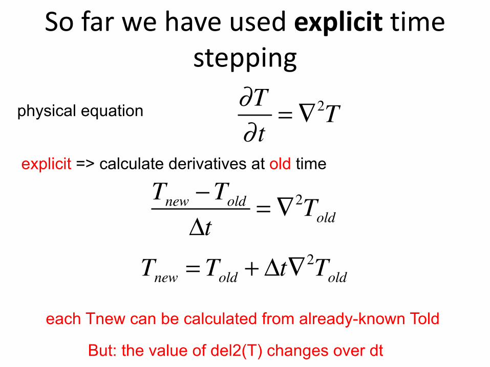
Sofarwehaveusedexplicit timestepping

∂T∂ t

= ∇2Tphysical equation

Tnew −ToldΔt

= ∇2Told

explicit => calculate derivatives at old time

But: the value of del2(T) changes over dt

Tnew = Told + Δt∇2Told

each Tnew can be calculated from already-known Told

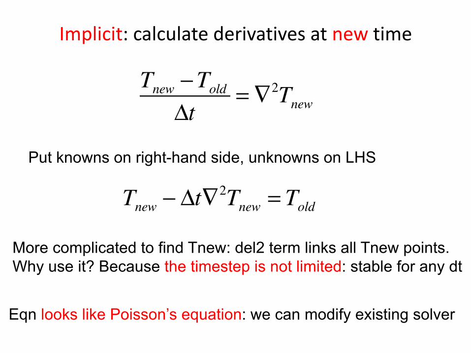
Implicit:calculatederivativesatnew time

Tnew −ToldΔt

= ∇2Tnew

Tnew − Δt∇2Tnew = Told

Put knowns on right-hand side, unknowns on LHS

More complicated to find Tnew: del2 term links all Tnew points.Why use it? Because the timestep is not limited: stable for any dt

Eqn looks like Poisson’s equation: we can modify existing solver

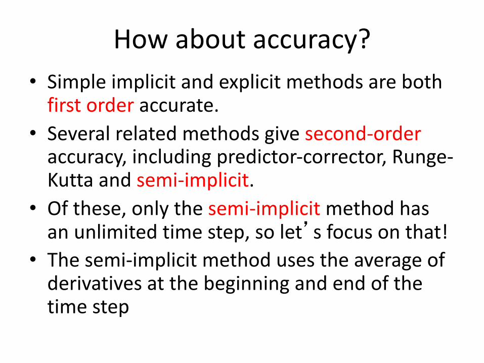
Howaboutaccuracy?• Simpleimplicitandexplicitmethodsarebothfirstorder accurate.

• Severalrelatedmethodsgivesecond-orderaccuracy,includingpredictor-corrector,Runge-Kuttaandsemi-implicit.

• Ofthese,onlythesemi-implicit methodhasanunlimitedtimestep,solet’sfocusonthat!

• Thesemi-implicitmethodusestheaverageofderivativesatthebeginningandendofthetimestep

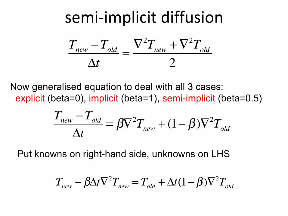
semi-implicitdiffusionTnew −Told

Δt= ∇2Tnew +∇

2Told2

Now generalised equation to deal with all 3 cases:explicit (beta=0), implicit (beta=1), semi-implicit (beta=0.5)

Tnew −ToldΔt

= β∇2Tnew + (1− β )∇2Told

Tnew − βΔt∇2Tnew = Told + Δt(1− β )∇2Told

Put knowns on right-hand side, unknowns on LHS

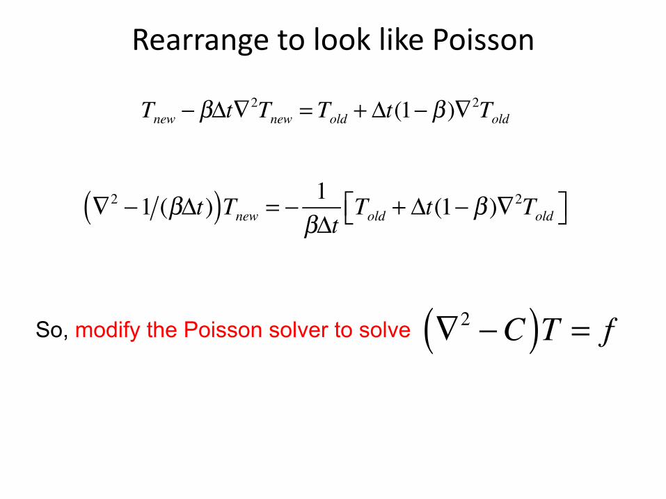
RearrangetolooklikePoisson

∇2 −1 (βΔt)( )Tnew = − 1βΔt

Told + Δt(1− β )∇2Told⎡⎣ ⎤⎦

So, modify the Poisson solver to solve ∇2 −C( )T = f

Tnew − βΔt∇2Tnew = Told + Δt(1− β )∇2Told

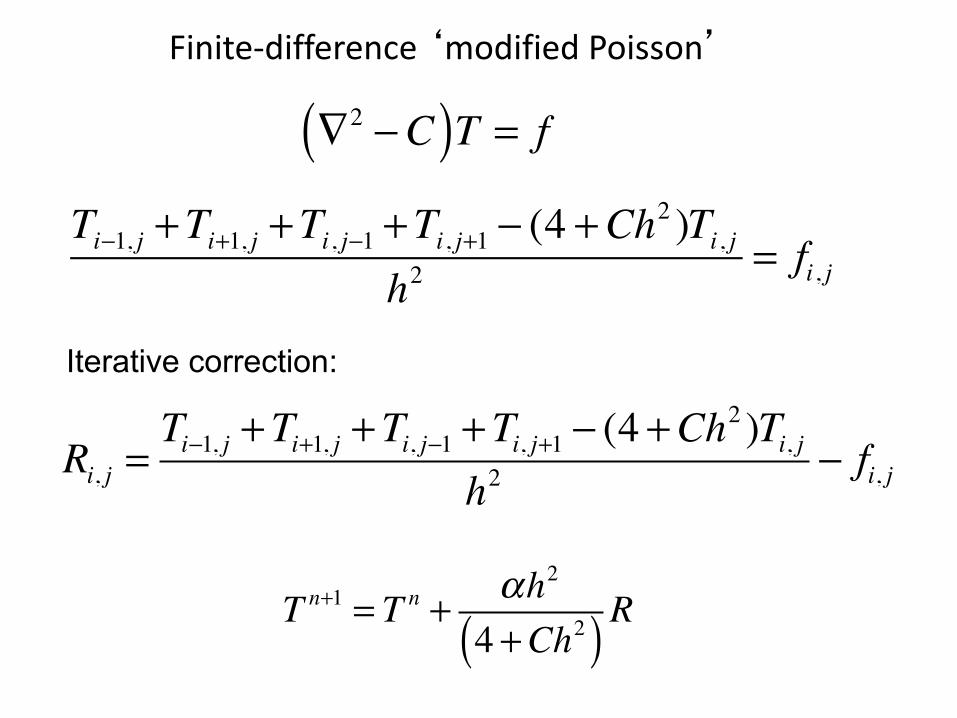
Finite-difference‘modifiedPoisson’

∇2 −C( )T = f

Ti−1, j +Ti+1, j +Ti, j−1 +Ti, j+1 − (4 +Ch2 )Ti, j

h2= fi, j

Iterative correction:

Ri, j =Ti−1, j +Ti+1, j +Ti, j−1 +Ti, j+1 − (4 +Ch

2 )Ti, jh2

− fi, j

T n+1 = T n + αh2

4 +Ch2( ) R

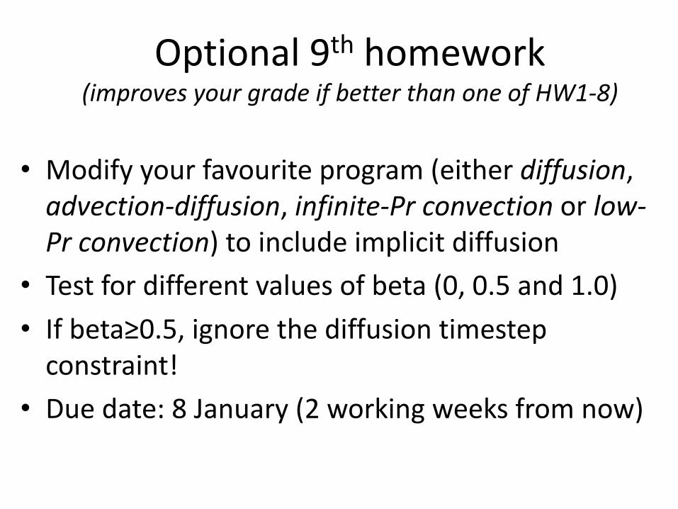
Optional9th homework(improvesyourgradeifbetterthanoneofHW1-8)

• Modifyyourfavourite program(eitherdiffusion,advection-diffusion,infinite-Pr convection orlow-Pr convection)toincludeimplicitdiffusion

• Testfordifferentvaluesofbeta(0,0.5and1.0)• Ifbeta≥0.5,ignorethediffusiontimestepconstraint!

• Duedate:8January(2workingweeksfromnow)

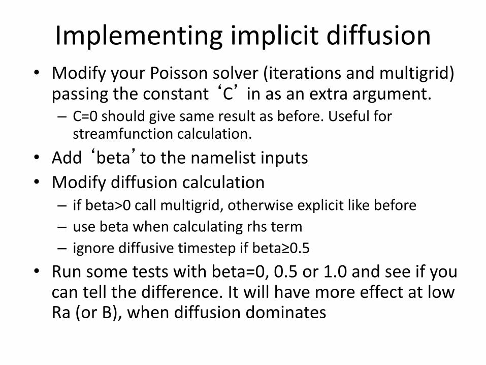
Implementingimplicitdiffusion• ModifyyourPoissonsolver(iterationsandmultigrid)passingtheconstant‘C’ inasanextraargument.– C=0shouldgivesameresultasbefore.Usefulforstreamfunctioncalculation.

• Add‘beta’tothenamelistinputs• Modifydiffusioncalculation

– ifbeta>0callmultigrid,otherwiseexplicitlikebefore– usebetawhencalculatingrhsterm– ignorediffusivetimestepifbeta≥0.5

• Runsometestswithbeta=0,0.5or1.0andseeifyoucantellthedifference.ItwillhavemoreeffectatlowRa(orB),whendiffusiondominates

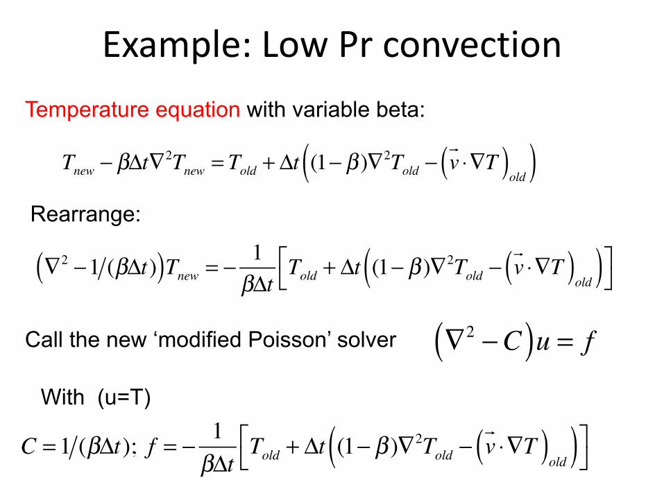
Example:LowPrconvection

Tnew − βΔt∇

2Tnew = Told + Δt (1− β )∇2Told − v!⋅∇T( )

old( )

∇2 −1 (βΔt)( )Tnew = − 1

βΔtTold + Δt (1− β )∇2Told − v

!⋅∇T( )

old( )⎡⎣

⎤⎦

∇2 −C( )u = f

C = 1 (βΔt); f = − 1

βΔtTold + Δt (1− β )∇2Told − v

!⋅∇T( )

old( )⎡⎣

⎤⎦

Temperature equation with variable beta:

Rearrange:

Call the new ‘modified Poisson’ solver

With (u=T)

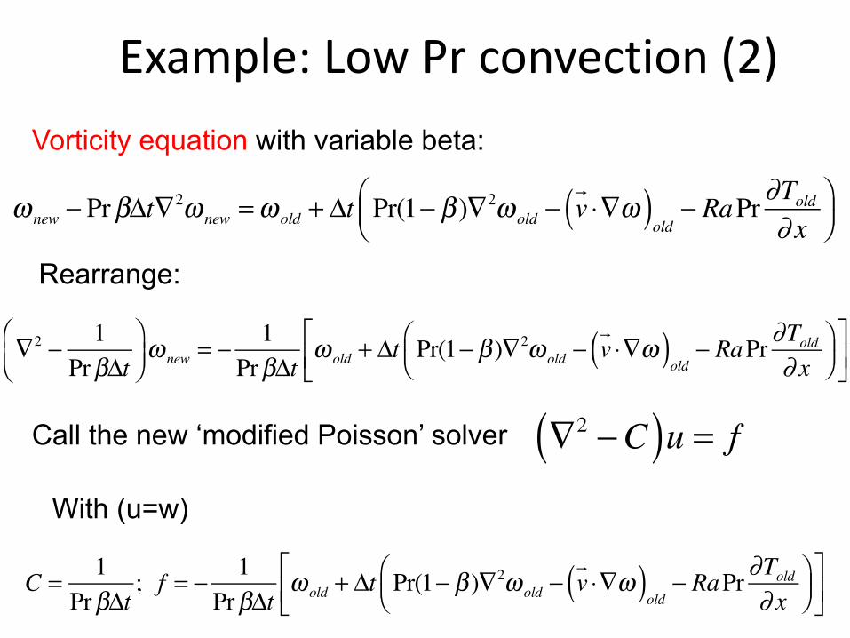
ω new − PrβΔt∇

2ω new =ω old + Δt Pr(1− β )∇2ω old − v!⋅∇ω( )

old− RaPr ∂Told

∂ x⎛⎝⎜

⎞⎠⎟

∇2 −C( )u = f ∇2 − 1

PrβΔt⎛⎝⎜

⎞⎠⎟ω new = − 1

PrβΔtω old + Δt Pr(1− β )∇2ω old − v

!⋅∇ω( )

old− RaPr ∂Told

∂ x⎛⎝⎜

⎞⎠⎟

⎡⎣⎢

⎤⎦⎥

Vorticity equation with variable beta:

Rearrange:

Call the new ‘modified Poisson’ solver

With (u=w)

Example:LowPrconvection(2)

C = 1

PrβΔt; f = − 1

PrβΔtω old + Δt Pr(1− β )∇2ω old − v

!⋅∇ω( )

old− RaPr ∂Told

∂ x⎛⎝⎜

⎞⎠⎟

⎡⎣⎢

⎤⎦⎥

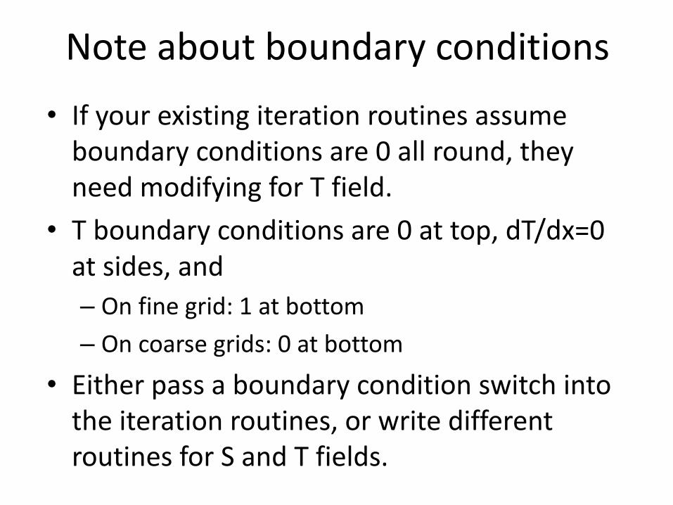
Noteaboutboundaryconditions• Ifyourexistingiterationroutinesassumeboundaryconditionsare0allround,theyneedmodifyingforTfield.

• Tboundaryconditionsare0attop,dT/dx=0atsides,and– Onfinegrid:1atbottom– Oncoarsegrids:0atbottom

• Eitherpassaboundaryconditionswitchintotheiterationroutines,orwritedifferentroutinesforSandTfields.

Handin

• Sourcecode• Resultsoftestcase(s)runusing

– differentvaluesofbetaand(ifbeta>0.5)– differenttimestepsincluding

• Timestep>diffusivetimestep

Usefullibrariesandothersoftware

• Forstandardoperationssuchasmatrixsolutionofsystemsoflinearequations,takingfast-Fouriertransforms,etc.,itisconvenienttodownloadsuitableroutinesfromsomefreelibrary,ratherthanwritingyourownfromscratch.

• Therearealsomorespecialisedfreeprogramsavailableforsomeapplications

• Alistisat:http://www.lahey.com/other.htm• Muchisavailableat:http://www.netlib.org/

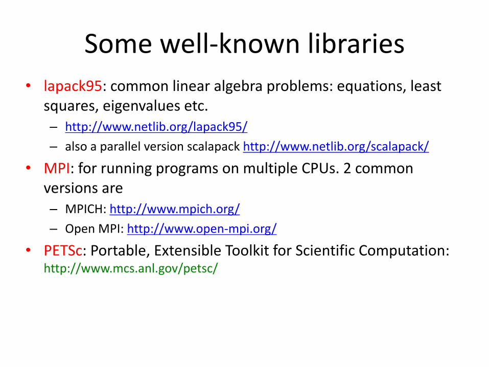
Somewell-knownlibraries• lapack95:commonlinearalgebraproblems:equations,least

squares,eigenvaluesetc.– http://www.netlib.org/lapack95/– alsoaparallelversionscalapack http://www.netlib.org/scalapack/

• MPI:forrunningprogramsonmultipleCPUs.2commonversionsare– MPICH:http://www.mpich.org/– OpenMPI:http://www.open-mpi.org/

• PETSc:Portable,ExtensibleToolkitforScientificComputation:http://www.mcs.anl.gov/petsc/

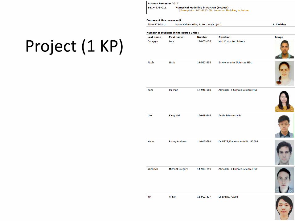
Project(1KP)

Project(optional,1KP)

1. Chosentopic,agreeduponwithme(suggestionsgiven,alsoasktheadvisorofyourMScorPhDproject).

– DueendofSemesterprüfung(17Feb2017)– Decidetopicbyfinallecture!– http://jupiter.ethz.ch/~pjt/FORTRAN/FortranProje

ct.html

Project:generalguidelines

• Choosesomethingeither– relatedtoyourresearchprojectand/or– thatyouareinterestedin

• Effort:1KP=>30hours.About4days’ work.• Icansupplyinformationaboutneededequationsandnumericalmethodsthatwehavenotcovered

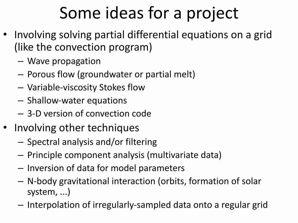
Someideasforaproject• Involvingsolvingpartialdifferentialequationsonagrid(liketheconvectionprogram)– Wavepropagation– Porousflow(groundwaterorpartialmelt)– Variable-viscosityStokesflow– Shallow-waterequations– 3-Dversionofconvectioncode

• Involvingothertechniques– Spectralanalysisand/orfiltering– Principlecomponentanalysis(multivariatedata)– Inversionofdataformodelparameters– N-bodygravitationalinteraction(orbits,formationofsolarsystem,...)

– Interpolationofirregularly-sampleddataontoaregulargrid

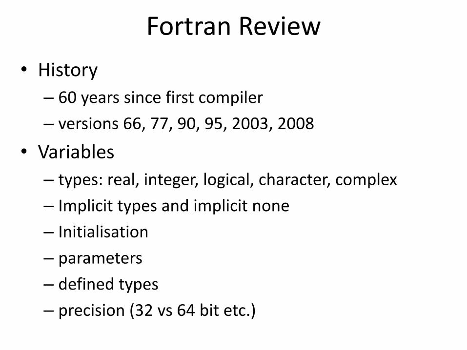
FortranReview• History

– 60yearssincefirstcompiler– versions66,77,90,95,2003,2008

• Variables– types:real,integer,logical,character,complex– Implicittypesandimplicitnone– Initialisation– parameters– definedtypes– precision(32vs64bitetc.)

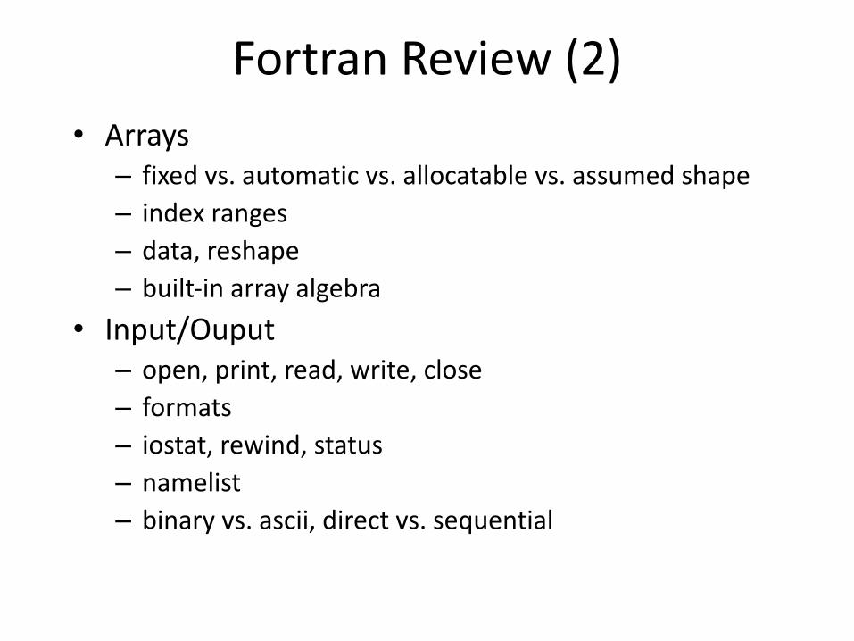
FortranReview(2)• Arrays

– fixedvs.automaticvs.allocatablevs.assumedshape– indexranges– data,reshape– built-inarrayalgebra

• Input/Ouput– open,print,read,write,close– formats– iostat,rewind,status– namelist– binaryvs.ascii,directvs.sequential

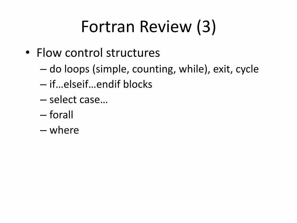
FortranReview(3)• Flowcontrolstructures

– doloops(simple,counting,while),exit,cycle– if…elseif…endifblocks– selectcase…– forall– where

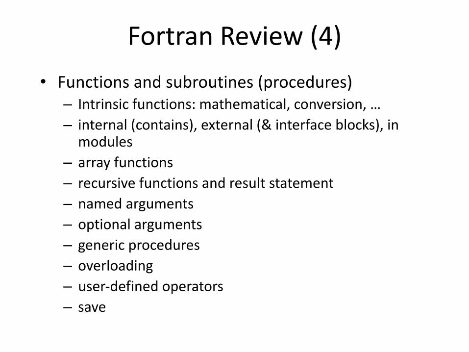
FortranReview(4)• Functionsandsubroutines(procedures)

– Intrinsicfunctions:mathematical,conversion,…– internal(contains),external(&interfaceblocks),inmodules

– arrayfunctions– recursivefunctionsandresultstatement– namedarguments– optionalarguments– genericprocedures– overloading– user-definedoperators– save

FortranReview(5)• Modules

– use– publicandprivatevariablesandfunctions– =>

• Pointers– tovariables,arrays,arraysections,areasofmemory,indefinedtypes

• Optimization– maximizeuseofcacheandpipelining– loopsmostimportant– 90/10rule(focusonbottlenecks)– avoidbranches,maximizedatalocality,unroll,tiling,…

• Libraries,makefiles

Foramoredetailedreview&discussion,see:

• https://www.tacc.utexas.edu/documents/13601/162125/fortran_class.pdf

NewfeaturesofFortran2003• Foradetaileddescriptionsee:ftp://ftp.nag.co.uk/sc22wg5/N1601-N1650/N1648.pdf

• Forasummary:http://www.fortran.bcs.org/2007/jubilee/newfeatures.pdf

• Enhancementstoderivedtypes– Parameterizedderivedtypes– Improvedcontrolofaccessibility– Improvedstructureconstructors– Finalizers

NewfeaturesofFortran2003(2)• Object-orientedprogrammingsupport

– Typeextensionandinheritance– Polymorphism– Dynamictypeallocation– Type-boundprocedures

• Datamanipulationenhancements– Allocatablecomponents– Deferredtypeparameters– VOLATILEattribute– Explicittypespecificationinarrayconstructors&allocatestatements

– Extendedinitializationexpressions– Enhancedintrinsicprocedures

NewfeaturesofFortran2003(3)• Input/outputenhancements

– Asynchronoustransfer– Streamaccess– Userspecifiedtransferopsforderivedtypes– Userspecifiedcontrolofrounding– Namedconstantsforpreconnectedunits– FLUSH– Regularizationofkeywords– Accesstoerrormessages

• Procedurepointers

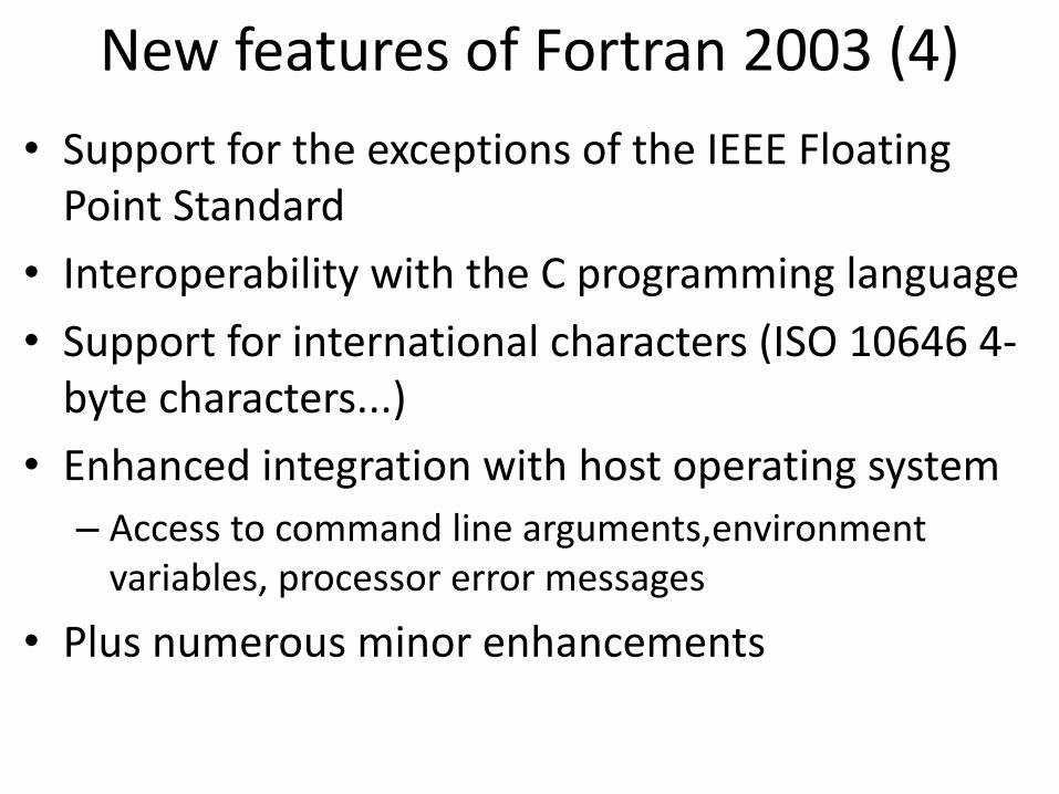
NewfeaturesofFortran2003(4)• SupportfortheexceptionsoftheIEEEFloatingPointStandard

• InteroperabilitywiththeCprogramminglanguage• Supportforinternationalcharacters(ISO106464-bytecharacters...)

• Enhancedintegrationwithhostoperatingsystem– Accesstocommandlinearguments,environmentvariables,processorerrormessages

• Plusnumerousminorenhancements

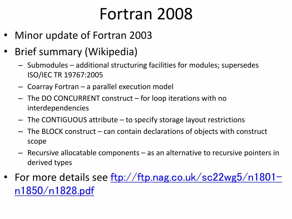
Fortran2008• MinorupdateofFortran2003• Briefsummary(Wikipedia)

– Submodules– additionalstructuringfacilitiesformodules;supersedesISO/IECTR19767:2005

– CoarrayFortran– aparallelexecutionmodel– TheDOCONCURRENTconstruct– forloopiterationswithno

interdependencies– TheCONTIGUOUSattribute– tospecifystoragelayoutrestrictions– TheBLOCKconstruct– cancontaindeclarationsofobjectswithconstruct

scope– Recursiveallocatablecomponents– asanalternativetorecursivepointersin

derivedtypes

• Formoredetailsseeftp://ftp.nag.co.uk/sc22wg5/n1801-n1850/n1828.pdf

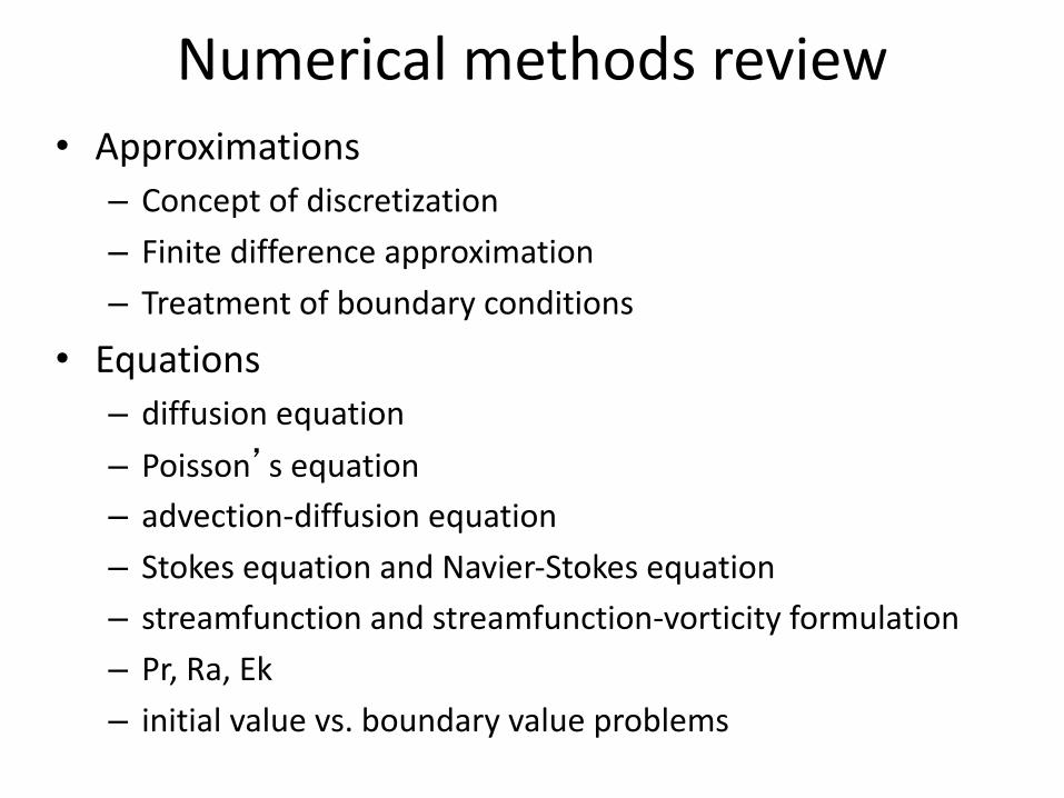
Numericalmethodsreview• Approximations

– Conceptofdiscretization– Finitedifferenceapproximation– Treatmentofboundaryconditions

• Equations– diffusionequation– Poisson’sequation– advection-diffusionequation– StokesequationandNavier-Stokesequation– streamfunctionandstreamfunction-vorticityformulation– Pr,Ra,Ek– initialvaluevs.boundaryvalueproblems

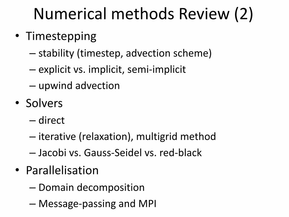
NumericalmethodsReview(2)• Timestepping

– stability(timestep,advectionscheme)– explicitvs.implicit,semi-implicit– upwindadvection

• Solvers– direct– iterative(relaxation),multigridmethod– Jacobivs.Gauss-Seidelvs.red-black

• Parallelisation– Domaindecomposition– Message-passingandMPI

Discussion

• Wehavefocussedononeapplication(constantviscosityconvection)

• Canapplysametechniquestootherapplications/physicalproblems

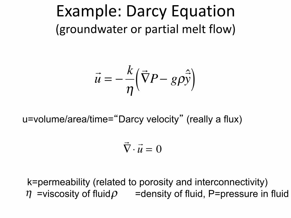
Example:DarcyEquation(groundwaterorpartialmeltflow)

�

∇ ⋅ u = 0

�

u = − k

η

∇ P− gρ

ˆ y ( )u=volume/area/time=“Darcy velocity” (really a flux)

k=permeability (related to porosity and interconnectivity)=viscosity of fluid, =density of fluid, P=pressure in fluidη ρ

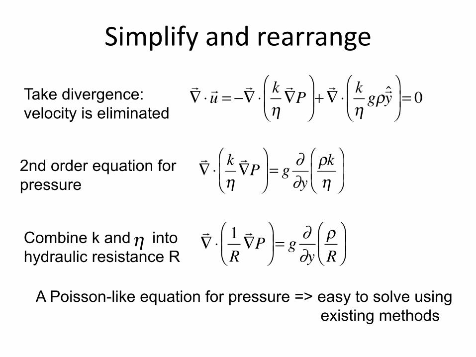
Simplifyandrearrange

�

∇ ⋅ u = −

∇ ⋅ k

η ∇ P

⎛

⎝ ⎜

⎞

⎠ ⎟ + ∇ ⋅ k

ηgρ ˆ y

⎛

⎝ ⎜

⎞

⎠ ⎟ = 0

�

∇ ⋅ k

η ∇ P

⎛

⎝ ⎜

⎞

⎠ ⎟ = g

∂∂y

ρkη

⎛

⎝ ⎜

⎞

⎠ ⎟

�

∇ ⋅ 1

R ∇ P

⎛ ⎝ ⎜

⎞ ⎠ ⎟ = g

∂∂y

ρR

⎛ ⎝ ⎜

⎞ ⎠ ⎟

Take divergence:velocity is eliminated

2nd order equation forpressure

Combine k and into hydraulic resistance R

A Poisson-like equation for pressure => easy to solve usingexisting methods

η

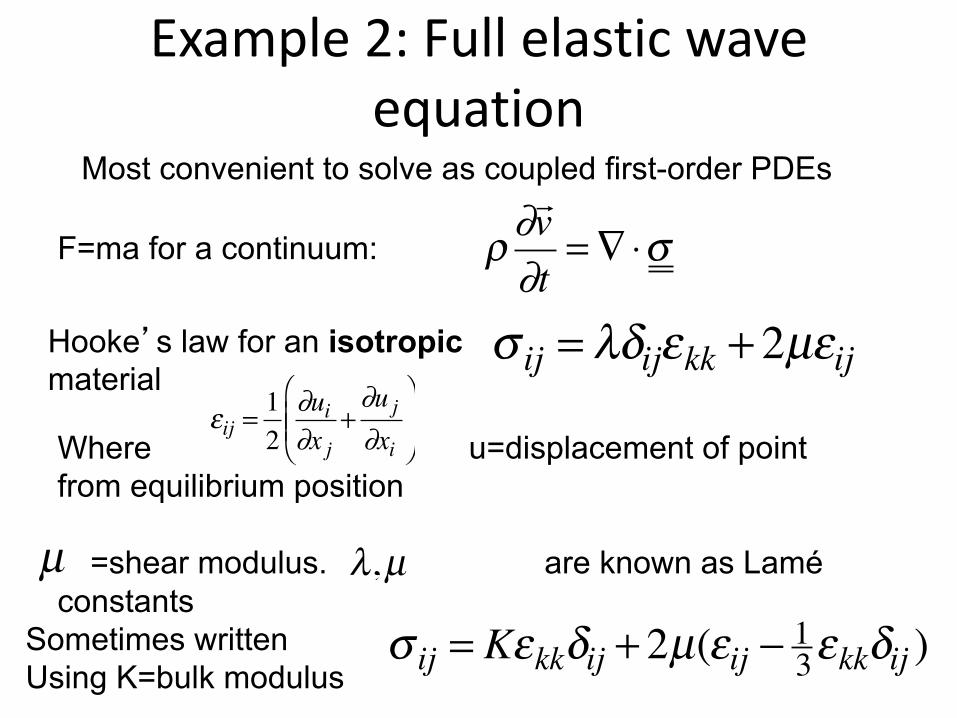
Example2:Fullelasticwaveequation

�

ρ ∂ v ∂t

= ∇⋅σ

�

σ ij = λδijεkk + 2µεij

F=ma for a continuum:

Most convenient to solve as coupled first-order PDEs

Hooke’s law for an isotropicmaterial

Where u=displacement of point from equilibrium position

=shear modulus. are known as Lamé constants

�

εij = 12

∂ui∂x j

+∂u j∂xi

⎛

⎝ ⎜ ⎜

⎞

⎠ ⎟ ⎟

�

σ ij = Kεkkδij + 2µ(εij − 13εkkδij )Sometimes writtenUsing K=bulk modulus

µ λ,µ

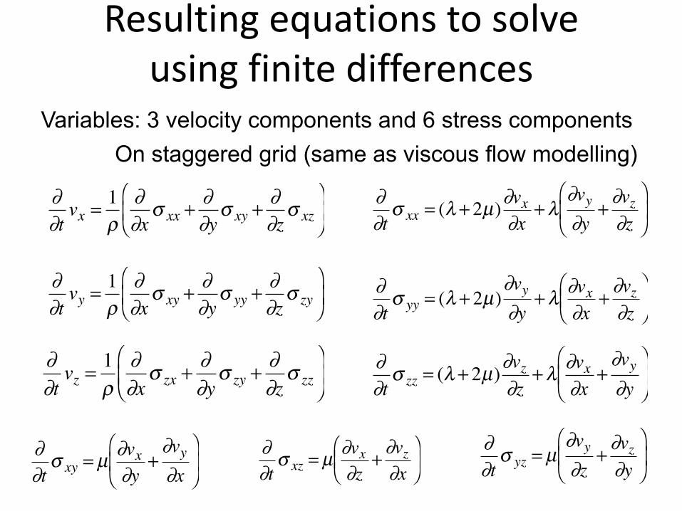
Resultingequationstosolveusingfinitedifferences

�

∂∂tvx = 1

ρ∂∂x

σ xx + ∂∂y

σ xy + ∂∂z

σ xz⎛

⎝ ⎜

⎞

⎠ ⎟

�

∂∂tvy = 1

ρ∂∂x

σ xy + ∂∂y

σ yy + ∂∂z

σ zy⎛

⎝ ⎜

⎞

⎠ ⎟

�

∂∂tvz = 1

ρ∂∂x

σ zx + ∂∂y

σ zy + ∂∂z

σ zz⎛

⎝ ⎜

⎞

⎠ ⎟

�

∂∂tσ xx = (λ + 2µ)∂vx

∂x+ λ

∂vy∂y

+ ∂vz∂z

⎛

⎝ ⎜

⎞

⎠ ⎟

�

∂∂tσ yy = (λ + 2µ)

∂vy∂y

+ λ ∂vx∂x

+ ∂vz∂z

⎛ ⎝ ⎜

⎞ ⎠ ⎟

�

∂∂tσ zz = (λ + 2µ)∂vz

∂z+ λ ∂vx

∂x+∂vy∂y

⎛

⎝ ⎜

⎞

⎠ ⎟

�

∂∂tσ xy = µ ∂vx

∂y+∂vy∂x

⎛

⎝ ⎜

⎞

⎠ ⎟

�

∂∂tσ xz = µ ∂vx

∂z+ ∂vz∂x

⎛ ⎝ ⎜

⎞ ⎠ ⎟

�

∂∂tσ yz = µ

∂vy∂z

+ ∂vz∂y

⎛

⎝ ⎜

⎞

⎠ ⎟

Variables: 3 velocity components and 6 stress componentsOn staggered grid (same as viscous flow modelling)

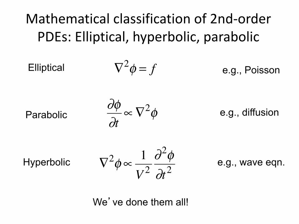
Mathematicalclassificationof2nd-orderPDEs:Elliptical,hyperbolic,parabolic

�

∇2φ = fElliptical

Parabolic

Hyperbolic

�

∇2φ ∝ 1V 2

∂2φ∂t2�

∂φ∂t

∝∇2φ

e.g., Poisson

e.g., diffusion

e.g., wave eqn.

We’ve done them all!

�

∇ ⋅ v = 0

�

∂T∂t

+ v ⋅ ∇T = ∇⋅ k∇T( )

�

∇ ⋅ k

η ∇ P

⎛

⎝ ⎜

⎞

⎠ ⎟ = g

∂∂y

ρkη

⎛

⎝ ⎜

⎞

⎠ ⎟

�

a i = Gm j x j − x i2

j=1

n, j≠i

∑ .( x j −

x i ) x j − x i

�

d2 x idt2

= a i

�

∂2P∂t2

= v2∇2P

�

1Pr

∂ v ∂t

+ v ⋅ ∇ v

⎛ ⎝ ⎜

⎞ ⎠ ⎟ = − ∇ P +

∇ ⋅ η ∂vi

∂x j+∂v j

∂xi

⎛

⎝ ⎜ ⎜

⎞

⎠ ⎟ ⎟

⎛

⎝ ⎜ ⎜

⎞

⎠ ⎟ ⎟ +

1Ek

Ω × v + Ra.T ˆ g

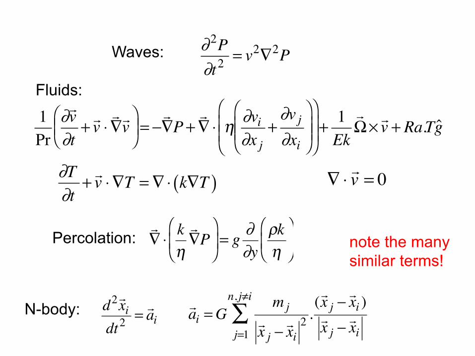
Waves:

Fluids:

Percolation:

N-body:

note the many similar terms!