Embed Size (px)
Citation preview

Continuum Mechanics and Thermodynamics (2012):http://link.springer.com/article/10.1007/s00161-012-0244-y
B. E. Abali · C. Vollmecke · B. Woodward · M. Kashtalyan ·I. Guz · W. H. Muller
Numerical modeling of functionally graded materials usinga variational formulationDedicated to Prof. Ingo Muller on the occasion of his 75th birthday
Received: date / Accepted: date
Abstract An approach of numerical modeling of heterogeneous, functionally graded materials, by usingthe finite element method, is proposed. The variational formulation is derived from the generic case so thatthe implementation of material coefficients, which are functions in space, is realized without any furtherassumptions. An analytical solution for a simple case is presented and used for validation of the numericalmodel.
Keywords Functionally graded materials· variational formulation· finite element method· heterogeneousmaterials
PACS 81.05.Ni· 46.25.Cc· 46.15.Cc
1 Introduction
Functionally graded materials (FGMs) have recently emerged as the new class of advanced composite mate-rials which show a gradual compositional variation of the constituents (e.g., metallic and ceramic) from onesurface of the material to the other resulting in continuously varying material properties [16]. The gradualvariation of material properties in FGMs is known to improvestructural integrity and performance while pre-serving the intended thermal, tribological, and/or structural benefits of the constituent materials. FGMs wereinitially developed for super-heat-resistant materials to be used in aeronautics or nuclear technology. Now, theFGM concept is being widely explored in a variety of engineering applications including functional materialsfor sensors and thermogenerators [17], dental and orthopaedic implants [20], and wear resistant coatings [24].FGMs can also be used for joining dissimilar materials [25].
Although FGMs are highly heterogeneous materials, it is useful to idealize them as continua with proper-ties that change smoothly with respect to spatial coordinates. A comprehensive review of principal develop-ments in modeling and analysis of functionally graded materials and structures is given by Birman and Byrd[3] covering homogenization of particulate FGMs, heat transfer issues, statics, dynamics, stability, fracture,testing, manufacturing and design.
As the use of FGMs increases, new methodologies have to be developed to analyze and design structuralcomponents made of them. The main issue encountered in application of the finite element method to FGMsis how to model a material with continuously varying properties. The simplest approach involves the use of
B. E. Abali, C. Vollmecke, W. H. MullerSchool V, Institute of Mechanics, Chair of Continuum Mechanics and Materials Theory, Technical University of Berlin, Sekr.MS2, Einsteinufer 5, 10587 Berlin, GermanyE-mail: [email protected]
M. Kashtalyan, B. Woodward, I. GuzSchool of Engineering, Fraser Noble Building (Room F030), University of Aberdeen, Aberdeen AB24 3UE, Scotland, UK
2 B. E. Abali et al.
homogeneous elements each with different properties, giving a stepwise change in properties in the directionof the material gradient. This approach has already been used by several researchers and can give reasonablyaccurate results. Etemadiet al. [6] modeled a sandwich panel with a functionally graded coresubject to lowvelocity impact. Zhanget al. [30] modeled the contact response of a functionally graded coating. Tilbrooket al. [26] and Wang and Nakamura [29] modelled the propagation of cracks in FGMs. There are, however,several problems in using this approach which are discussedby Buttlaret al. [4]. Due to the model approx-imating the continually varying properties of the materialwith stepwise changes, a computational error isalways introduced, particularly in cases of high stiffnessgradients. In order to minimize this error, a very finemesh in the direction of the property gradient is often required. This can, however, lead to extremely longcomputation times.
A more advanced method of including property variation intoa finite element model is to use elementswhich themselves contain a gradient in properties. Santareand Lambros [23] proposed a 2-D graded elementwith material properties evaluated directly at the GAUSS point. An alternative approach was adopted by Kimand Paulino [13], who have proposed a fully isoparametric element formulation that interpolates materialproperties at each GAUSS point from the nodal values, using the same shape functions as the deformations.Comparisons of 2-D graded and homogenous elements under various loading conditions with analytical so-lutions in the literature showed that graded elements give far greater accuracy when modeling FGMs [13].
In this paper, the mathematical representation of the Galerkin finite element method is derived upon avariational formulation and position dependent properties are directly integrated. Therefore, without any needof an element reformulation or reimplementation in the isoparametric space, the equations can be solved byusing a various collection of novel algorithms from the FEniCS project [10], which are all released under opensource GNU public license [7]. Moreover, a simple geometry and appropriate boundary conditions lead to ananalytic solution which is used for verification of the approach. The advantage of that approach is that thematerial properties are approximated in the same functional space as the solution such that the same accuracycan be achieved.
At the beginning of the paper, the analytical solution is briefly outlined as derived in [11]. Then, startingwith the variational formulation for the generic case, the specific problem, a simply supported plate un-der sinusoidal loading, is deduced. This allows to show the assumptions to be made and clarifies how thediscretization of the material coefficients naturally arises. Subsequently, the numerical results are validatedagainst the analytical solution and parametric studies arepresented. Having a verified finite element code willallow engineers to compute complex geometric structures with FGMs and therefore, the code is presentedunder GNU public license in [1].
2 Problem statement
In order to determine the distribution of displacementsui , in a linear elastic solid body, field equations ofelasticity theory and boundary conditions are required. Without discussing their generality for the moment,we assume linear kinematic relations:
εi j =∂u(i∂Xj)
=12
( ∂ui
∂Xj+
∂uj
∂Xi
)
, (1)
equilibrium equations:
∂ σi j
∂Xj= 0 , (2)
and a linear elastic constitutive HOOKE’s law for isotropic materials:
σi j =2Gν
1−2νεδi j +2Gεi j , (3)
whereεi j are the components of the strain tensor,ε = ∂ui∂Xi
is the volumetric strain or dilatation,σi j are the com-ponents of the stress tensor, andν andG are POISSON’s ratio and shear modulus, respectively. EINSTEIN’s

Numerical modelling of FGMs 3
summation convention is employed throughout. It should be pointed out that for FGMs the material coeffi-cients are no longer constants but functions of the materialcoordinate systemXi = (X1,X2,X3), thus materialis heterogeneous. Here, the geometry is a plate with its thickness directionX3. Since a variation of POISSON’sratio normally does not play a significant role in determining the magnitudes of stresses and displacements inFGMs, POISSON’s ratioν is commonly assumed to be constant,i.e., ν = const. [22]. The shear modulusG isassumed to depend only on thickness,X3. Even these simplified assumptions lead to a more complex problemthan in the case of homogeneous materials.
Equations (1)-(3) form a set of 15 coupled partial differential equations for 15 unknowns. The number offield equations and unknowns can be reduced to three if the displacement formulation is used. For isotropicFGMs the equilibrium equations in terms of displacements can be written, as [19]:
G∆u1+G
1−2ν∂ ε∂X1
+( ∂u1
∂X3+
∂u3
∂X1
) ∂G∂X3
= 0 ,
G∆u2+G
1−2ν∂ ε∂X2
+( ∂u2
∂X3+
∂u3
∂X2
) ∂G∂X3
= 0 , (4)
G∆u3+G
1−2ν∂ ε∂X3
+ εd
dX3
( 2Gν1−2ν
)
+2∂u3
∂X3
dGdX3
= 0 ,
where∆ = ∂ 2
∂X21+ ∂ 2
∂X22+ ∂ 2
∂X23
denotes the Laplacian. For homogeneous materials, terms involving first-order
derivatives of the material coefficients will vanish, and the equations, Eqs. (4), will reduce to the well-knownNAVIER-LAM E equations.
The system of Eqs. (4) is still difficult to solve, and additional mathematical techniques have been devel-oped for further simplification. One of the commonly used methods employs the use of displacement potentialfunctions, which establish a representation for the displacements that automatically satisfies the equilibriumequations in terms of displacements. Equations (4), can be decoupled in terms of displacements [19] yieldingto the following two equations for the displacement functionsL = L(X1,X2,X3) andN = N(X1,X2,X3):
∆(
1G
∆L
)
−1
1−ν
(
∆−∂ 2
∂X23
)
Ld2
dX23
(
1G
)
= 0 , ∆N+g(X3)∂N∂X3
= 0 , g(X3) =d
dX3lnG(X3) . (5)
The displacements can then be represented in terms ofL = L(Xi) andN = N(Xi) as (cf., [19]):
u1 =−1
2G
(
ν∆−∂ 2
∂X23
)
∂L∂X1
+∂N∂X2
,
u2 =−1
2G
(
ν∆−∂ 2
∂X23
)
∂L∂X2
−∂N∂X1
, (6)
u3 =−1G
(
ν∆−∂ 2
∂X23
)
∂L∂X3
+∂
∂X3
[
12G
(
ν∆−∂ 2
∂X23
)
L
]
.
4 B. E. Abali et al.
By virtue of HOOKE’s law, Eq. (3), the stresses in an isotropic linearly elastic FGM with constantν andthickness dependentG(X3) can be expressed in terms of displacement functions as follows:
σ11 =
(
ν∂ 2
∂X22
∆+∂ 4
∂X21 ∂X2
3
)
L+2G∂ 2N
∂X1∂X2,
σ22 =
(
ν∂ 2
∂X21
∆+∂ 4
∂X22 ∂X2
3
)
L−2G∂ 2N
∂X1∂X2,
σ33 =
(
∆−∂ 2
∂X23
)2
L , (7)
σ13 =−
(
∆−∂ 2
∂X23
)
∂ 2L∂X1∂X3
+G∂ 2N
∂X2∂X3,
σ23 =−
(
∆−∂ 2
∂X23
)
∂ 2L∂X2∂X3
−G∂ 2N
∂X1∂X3,
σ12 =−
(
ν∆−∂ 2
∂X23
)
∂ 2L∂X1∂X2
−G
(
∂ 2
∂X21
−∂ 2
∂X22
)
N .
Plevako’s displacement functions were recently revisitedby Kashtalyan and Rushchitsky [12] who used aprocedure similar to his and developed displacement functions for a transversely isotropic FGM.
Depending on the nature of the heterogeneity of the materialand the boundary conditions on the surfaceof the solid, the solution of Eqs. (4) or Eqs. (5) could becomequite complex which limits the applicabilityof analytical methods. However, in some cases it is still possible to generate an analytical solution for the3-D elasticity boundary-value problem for FGMs by using thedisplacement functions. One of these cases isa simply supported rectangular plate subjected to transverse loading, with exponential variation of the shearmodulus through the thickness.
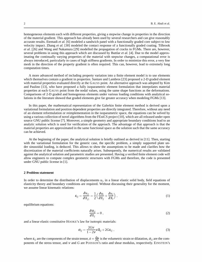
Fig. 1: Plate as a three-dimensional continuum under sinusoidal loading.
For this purpose, consider a plate of lengtha, width b and thicknessh, referred to a Cartesian co-ordinatesystemXi = (X1,X2,X3) in material configuration so that 0≤ X1 ≤ a, 0≤ X2 ≤ b and 0≤ X3 ≤ h (Fig. 1). The

Numerical modelling of FGMs 5
material of the plate is a FGM with a constant POISSON’s ratioν, and a shear modulusG varying exponentiallythrough the thickness fromG0, the value at the bottom surface, toG1, the value at the top surface, accordingto:
G(X3) = G1exp
(
γ(X3
h−1
)
)
, γ = lnG1
G0, ν = const., (8)
whereγ is the inhomogeneity parameter. At the edges of the plate, Navier-type boundary conditions areassumed such that:
(X1 = 0 , X2 , X3)∨ (X1 = a , X2 , X3) : σ11 = 0 , u2 = u3 = 0 , (9)
(X1 , X2 = 0 , X3)∨ (X1 , X2 = b , X3) : σ22 = 0 , u1 = u3 = 0 .
The boundary conditions, Eqs. (9), are representative of roller supports and analogous to simply supportededges used in plate theories. The top surface of the plate is subjected to transverse loading:
(X1 , X2 , X3 = h) : σ33 = Q=−qsinπmX1
asin
πmX2
b, σ31 = σ32 = 0 , (10)
wheremandn are wave numbers andq is the loading coefficient. The bottom surface of the plate isload-free,i.e.:
(X1 , X2 , X3 = 0) : σ33 = σ32 = σ31 = 0 . (11)
An analytical solution to the above-stated boundary value problem was obtained in [9] by using the displace-ment functions method. It is presented in the Appendix for the sake of completeness.
3 Variational formulation
As outlined in the last section, an analytic solution can sometimes be obtained for a particular case of geom-etry, boundary and loading conditions, specifically for a rectangular plate with simply-supported edges andtransverse sinusoidal loading as shown in Fig. 1. For practical purposes other geometries and conditions areof interest, which may be approximated numerically. In thispaper, the widely known Finite Element Method(FEM), as an approximation in space is implemented. We proceed to discuss its peculiarities in the presentcase.
Any functionψ(XXX, t), defined in space and time, is separated into a time dependentand a space dependentfunction:
ψ(XXX, t) =∑ID
Ψ ID(t)φ ID(XXX) . (12)
This is undertaken for every nodal point with a unique identification number, ID. The space functionφ ID(XXX)determines the connection of the nodal points, thus it depends solely on the geometry. The time functionΨ ID(t) represents the values of the functionψ(XXX, t) in each node. The value in each node has an influence ina finite domain, thusφ ID(XXX) has a local support. This local support, a functional space spanned over the affineconnections{φ1,φ2, . . . ,φnode nr.}, is a HILBERT configurationH as defined in [9]. We choose to use linearspace functionsφ ID(XXX) so that theH configuration can be represented by a set of oblique axes. By choosingoblique axes, we need to distinguish between co-and contravariant notation, so that the contravariant compo-nentsXk of the absolute vectorXXX are parallel projections to the axes.
The problem can appropriately be modeled as a closed system,which led us to choose material frame-work, i.e., coordinatesXk label particles. The usual continuum mechanics notation (see [5,27]) is applied.However, for simplicity, the configurationH will not be mentioned explicitly, thus we writeψ(Xk, t) whilewe meanψ
H
(Xk, t) for all the functions in that section.
A 3-D body in the known reference stateB0 will be deformed under given loading conditions. The ob-jective is to find the equation of the displacement fieldui which is the difference between the reference and

6 B. E. Abali et al.
the deformed state of the body,B0 andB, respectively. Both are closed domains. Thus particles arenot per-mitted to accumulate nor disintegrate, and identifiable by the material coordinatesXi . The coordinates of theparticlesXi are known in the reference frame, which is the undeformed body B0 itself. Furthermore, the dis-placements must not violate the conservation laws. Hence wecan start off the conservation laws and end upwith the equations for which the analytical solution is found. The usual assumptions in linear elasticity theoryallow to employ a heterogeneous material. In order to justify and in addition to assure that the formulationfor the numerical approximation does not contradict these assumptions, we briefly review the origin of Eq. (2).
The balance of mass and linear momentum read in the deformed state:
ddt
∫
B
ρ dV = 0 ,ddt
∫
B
ρυi dV =
∫
∂Bnj σ ji da+
∫
B
ρ fi dV , (13)
where the mass densityρ, velocitiesυi and body forcesfi are the numerical values of corresponding func-tions. Moreover, plane normal on the surfacenj and momentum fluxσ ji , given by the CAUCHY stress tensor,refer to the deformed state,B. Of course, Eq. (13) can also be expressed in the reference stateB0, to whichthe coordinatesXi refer. The sought displacementsui are then the difference of the coordinates in the de-formed statexi and the coordinates in the undeformed,i.e., reference, stateXi . The volume element dV in thedeformed stateB is related to the volume element dV0 in the undeformed stateB0 by [18, p. 62] :
dV = det( ∂xi
∂X j
)
dV0 = JdV0 , (14)
whereJ stands for Jacobian and measures the deviation of the configuration from the reference state. Anal-ogously, the relation between the area element dA in B and the area element dA0 in B0 can be obtainedas:
ni da= dai =
(
∂xi
∂Xr
)−1
JNr dA0 , (15)
whereNr represents normals to the tangent plane on the surface inB0. Consequently, by substituting Eqs. (14)and (15) into Eq. (13) and implementing the conservation of mass, such thatρ0 = ρ/J = const.|t holds, thebalance law for linear momentum can be rewritten in the material configurationB0 as follows:
∫
B0
ρ0∂ υi
∂ tdV0 =
∫
∂B0
σ ji
(
∂x j
∂Xr
)−1
JNr dA0+∫
B0
ρ0 fi dV0 . (16)
Eq. (16) holds in general for all closed systems. However, for our problem, firstly the inertia termρ0∂ υi/∂ tis neglected while the problem is assumed to be modeled accurately using stationarity. Secondly, the bodyforces fi are ignored and deflection of the body under its own weight, caused by gravitation, is neglected.Subsequently, Eq. (16) reads:
0=
∫
∂B0
σ ji
(
∂x j
∂Xr
)−1
JNr dA0 . (17)
Analogously to the analytic solution, which stems from the static theory of linear elasticity, the assumption ofsmall displacements is applied:
∂x j
∂Xr ≈ δ jr , J = det( ∂x j
∂Xr
)
≈ 1 . (18)
Moreover, continuity of stress within the body is assumed. Although the material is heterogeneous, it doesnot contain any singular surfaces. Hence, by applying the GAUSS’ theorem, the latter equation yields to theequilibrium condition (2) used in Section 2:
0=
∫
∂B0
σ riNr dA0 =
∫
B0
∂ σ ri
∂Xr dV0 ⇒∂ σ r
i
∂Xr = 0 . (19)

Numerical modelling of FGMs 7
According to the RIESZ representation theorem, any test functionwi of the same rank as the integrand(here a tensor of first order) can be chosen to contract the latter equation to an invariant under configurationtransformation [21]:
0=
∫
B0
∂ σ ri
∂Xr wi dV0 , (20)
such that it holds under deformed and undeformed states. Since the choice of the test functions is arbitrary,defining them as:
wi = ∑ID
1IDφ ID(Xi) , (21)
is admissible. This is also known as the GALERKIN method. In order to integrate Eq. (20) in a discrete sense,GAUSS quadrature is used:
∫
B0
f dV0 =n+1
∑i
f |pi g|pi , f =∂ σ r
i
∂Xr wi , (22)
i.e., we obtain a sum of products of the discrete function valuesf |pi and weight function valuesg|pi overn+1tabulated integration points,pi , which were first determined by GAUSS and are known as GAUSSpoints in theliterature. They depend on the polynomial ordern, which is determined by the element type. Here we chooselinear elements, thus two GAUSS points in each direction are sufficient for a numerical integration.
However, calculating these points and their weights may be cumbersome. Since integration is additive, itcan be evaluated in finite subdomainsBe
0 and then summed up:
0=
∫
B0
∂ σ ri
∂Xr wi dV0 =⋃
e
∫
Be0
∂ σ ri
∂Xr wi dV0 . (23)
Every finite subdomain can be mapped into a geometrically identical subdomain (isoparametric element) uponwhich the GAUSS points and their weights are calculated and tabulated only once and where the integrationaccording to Eq. (22) takes place. Hence every function can be projected into discretized space and evaluatedat the GAUSS points which is a beneficial advantage when using the open source code FEniCS [14].
Traditionally, in conventional FEM software, the materialcoefficients are defined as constants per element.Therefore, modeling functionally graded materials accurately is inevitably highly mesh dependent. Owing tothe evaluation at the GAUSS points, utilizing FEniCS has the major advantage that any function can be evalu-ated in the same order of continuity in the discrete system aspreviously defined over the whole domain.
Equivalent to the formulation in the Section 2 linear symmetrical strains are introduced as follows:
ε ij =
∂u(i
∂X j)=
12
(
∂ui
∂X j +∂uj
∂Xi
)
(24)
and the constitutive relation is defined by HOOKE’s law
σ ij =Ci l
jk εkl , (25)
with an elasticity tensor of rank four. For the isotropic case, it can be described with two LAM E coefficients:
Ci ljk = λδ i
j δ lk +µ(δ i
kδ lj +δ il δ jk) , (26)
or with the widely known engineering material coefficients,YOUNG’s modulusE, shear modulusG, andPOISSON’s ratioν:
λ =Eν
(1+ν)(1−2ν)=
2Gν(1−2ν)
, µ =E
2(1+ν)≡ G . (27)

8 B. E. Abali et al.
Upon substitution of the kinematic and constitutive relation, the variational form in Eq. (23) can be rewrittenin the interior of the domain, thus:
0=
∫
B0
∂∂Xr
(
2Gν(1−2ν)
δ ri∂uk
∂Xk +2G∂u(r
∂Xi)
)
wi dV0 . (28)
In general, boundary conditions are given in terms of the displacement on the boundary∂BD (DIRICHLETtype) or in terms of the loading on the boundary∂BN (NEUMANN type):
ui = ui(Xk) = ui , ∀Xk ∈ ∂BD , (29)
Nrσ ri =
2Gν(1−2ν)
Ni∂uk
∂Xk +2GNr∂u(r
∂Xi)= ti , ∀Xk ∈ ∂BN ,
where∂BD ∩∂BN = {} and∂B= ∂BD ∪∂BN. The problem is well-defined if the conditions from Eq. (29)∫
∂BD
(ui − ui)dA0 = 0 ,
∫
∂BN
(
Nrσ ri − ti
)
dA0 = 0 (30)
hold. By contracting with the same test functions (cf., Eq. (21)) and by adding these terms to Eq. (20), thefollowing variational form results:
∫
∂BD
(ui − ui)wi dA0+
∫
∂BN
(
Nrσ ri − ti
)
wi dA0 =
∫
B0
∂ σ ri
∂Xr wi dV0 . (31)
The chosen configurationH is linear in each finite element, in other words, functions are allowed to bepolynomials of degree one. Thus the right side of Eq. (31), with the second order derivatives inui , cannot beadequately represented. This can be rectified by applying the GAUSS-OSTROGRADSKIY theorem (integrationby parts for tensors):
∫
∂BD
(ui − ui)wi dA0+
∫
∂BN
(Nr σ ri − ti)w
i dA0 =−
∫
B0
σ ri∂wi
∂Xr dV0+
∫
∂Bσ r
iwiNr dA0 , (32)
since∂B= ∂BD ∪∂BN , it follows:∫
∂BD
(ui − ui −σ riNr )w
i dA0−∫
∂BN
tiwi dA0 =−
∫
B0
σ ri∂wi
∂Xr dV0 . (33)
By deriving Eq. (33), the coefficients were allowed to be functions in space. Finally, if test functionswi areimplemented such that they vanish on the DIRICHLET type boundaries,i.e., wi
∣
∣
∂BD= 0, and by using the
same boundary conditions as in Eqs. (9), (10), (11), the variational form reads:
−
∫
∂Btop
QNiwi dA0+
∫
B0
2Gν(1−2ν)
∂uk
∂Xk
∂wi
∂Xi dV0+
∫
B0
2G∂u(r
∂Xi)
∂wi
∂Xr dV0 = 0 , ∂Btop = (X1 , X2 , X3 = h) .
(34)
This is the system of linear equations which has been programmed and solved by using the FEniCS project[14,10,15]. The visualization was undertaken with Paraview [8]. The code is supplied under GNU publiclicense in [1].
4 Validation and results
In this section the previously described numerical solution of the variational formulation is first tested for con-vergence. The model geometry is as explained in Section 2. The NEUMANN and DIRICHLET type boundariesas defined in Eqn.s (9),(10),(11) are implemented. After theconvergence test, results are presented for variousvalues of the heterogeneity parameterγ (cf., (8)2). According toγ there is a neutral surface, along which existzero displacements. The material is chosen to be heterogeneous only in the direction of thickness,i.e., X3.Therefore the neutral surface is a plane, parallel to theX1X2 plane. If the parameterγ is set equal to zero, theneutral plane happens to be in the middle, as known from platetheory.

Numerical modelling of FGMs 9
4.1 Convergence
As discussed in Section 3, employing the variational formulation in the numerical assessment allows the shearmodulus to be defined as a function of position,i.e., G(Xi). Having applied the relevant boundary conditions,the variational form in Eq. (34) is well-posed and can be solved by using the finite element method. The solu-tion is an approximation, thus there is an discrepancy between the numerical solution and the analytical one,and the error depends on two choices. Firstly, it depends on the configuration, how the solution is discretized,i.e., on the space functionsφ ID(Xk) in Eq. (12) which spans the HILBERT configurationH, equipped with anL2 norm [9]. Secondly, the error depends on the size of the finiteelements, related to the size of the local sup-port where the nodal value has influence. Since every function, including the material coefficient functions, isdefined on the same configuration, the error of the approximation depends only on the size of the elements.Hence if the error reduces globally, which is achieved by increasing the number of elements, the numericalapproximation will converge to the analytical solution asymptotically.
In order to test the convergence, a box of 5m×5m×1m is modeled with the same number of elements ineach direction, which is increased linearly from 10 to 50 in five steps. Material properties are chosen such thata nickel/alumina FGM [2] is realized with Al2O3 on top,E1 = 393.0 GPa, and Ni on bottom,E0 = 199.5 GPa,so that the inhomogeneity parameterγ and Poisson’s ratioν read:
ν = 0.3 , γ = lnG1
G0= ln
E1
E0= 0.6780, G1 =
E1
2(1+ν). (35)
The convergence test for increasing degrees of freedom (DOF) can be seen in tabulated form in Table 1. Theerror is the discrepancy between the analytical (exact)ue
i and numerical (approximate)ui solution:
erri = uei −ui . (36)
As theH configuration proposes theL2 norm, its error has the size:
‖erri‖L2 =
∫
B0
erri erri dV0 . (37)
However, this depends on the chosen volume. Therefore the density of it is a more appropriate quantity to usefor the convergence,i.e., :
errL2 =‖erri‖L2∫
B0dV0
. (38)
Moreover, the quantity inL2 norm has not a physical meaning. For practical purposes, it is more helpful tocalculate the maximum of the error as follows:
errmax= max(
erri = uei −ui in B0
)
, (39)
which is the maximum error existing in the whole body. By increasing the number of elements in the bodythe position of the maximum error might change, thus it does not measure the convergence. Hence, for theconvergence, emphasis is put upon the error density in theL2 norm.
Nr. of elements in each direction Degrees of freedom errmax errL2
10 3993 0.389 12.252e-0720 27783 0.128 3.998e-0730 89373 0.066 1.937e-0740 206763 0.042 1.161e-0750 397953 0.031 0.792e-07
Table 1: Results for the error in maximum norm,errmax, and density of the error inL2 norm,errL2, stemmingfrom the convergence analysis. The values approach zero forincreasing number of DOF.
Theoretically, once the error converges to zero, the numerical model is validated, since the finite elementmethod has the analytical solution as its upper bound. Therefore, the model is validated against the analytical

10 B. E. Abali et al.
solution since the values in Table 1 clearly demonstrate theconvergence of the model while theL2 normprogresses towards zero. The quality of the accuracy,i.e., the maximum of the error, depends on the problemspecifications and can be improved by increasing the number of elements. Fig. 2 shows the displacement, onecomponent of the stress tensor and theVON M ISESequivalent stress distribution of the body when using therealistic material properties from above and a lateral traction amplitude ofQ= 10 MPa. The correspondingresponses are as expected and manifest the reliability of the numerical results.
(a) (b)
(c) (d)
Fig. 2: Distribution of the magnitude of the displacement, (a) in deformed shape(1 : 1), (b) in deformed shapewith scaled displacements for visualization(1 : 800). Distribution (c) of the stress componentσ12 and (d) oftheVON M ISESequivalent stress.
4.2 Results
In the previous paragraph the convergence for 397953 DOF (cf., Table 1) has been demonstrated and vali-dated. Further cases can now be investigated. In particular, the effects of changing values of the heterogeneityparameterγ will now be analyzed and discussed. In Table 2, the results ofthe numerical solution for the lateraldeflectionu3 at the midpoint,i.e., (a/2,b/2,h/2), for varying values ofγ from -2 to 2 are compared to theanalytical solutionue
3 from Section 2. It can be noted that the relative error is sufficiently small for typicalengineering applications which demonstrates the accuracyof the model. Furthermore, it should be pointedout here, that the relative error does not depend on the heterogeneity parameterγ . If γ tends towards zerothe material becomes homogeneous. Therefore approaching the homogeneous solution from top and bottom

Numerical modelling of FGMs 11
γG1
G0=
E1
E0ue
3(a/2,b/2,h/2) u3(a/2,b/2,h/2) relative error
2.0 7.3891 −3.697 −3.680 0.00451.0 2.7183 −2.261 −2.235 0.01110.5 1.6487 −1.745 −1.731 0.00820.1 1.1052 −1.415 −1.406 0.00610.01 1.0101 −1.350 −1.341 0.006110−3 1.0010 −1.343 −1.335 0.006110−4 1.0001 −1.343 −1.335 0.006110−5 1.0000 −1.343 −1.334 0.0061−10−5 1.0000 −1.343 −1.334 0.0061−10−4 0.9999 −1.343 −1.334 0.0061−10−3 0.9990 −1.342 −1.334 0.0061−0.01 0.9901 −1.336 −1.328 0.0061−0.1 0.9048 −1.274 −1.266 0.0062−0.5 0.6065 −1.034 −1.025 0.0083−1.0 0.3679 −0.794 −0.784 0.0118−2.0 0.1353 −0.456 −0.455 0.0026
Table 2: Qualitative comparison of the results for the lateral deflection of the analyticalue3 and numerical
solutionsu3, at the midpoint(a/2,b/2,h/2) of the geometry.
sides,i.e., by varyingγ > 0 andγ < 0, sheds light on the versatility of the numerical model. Theanalyticsolution for the homogeneous case has been proven and is wellestablished [28].
Fig. 3 illustrates the shift of the neutral plane for two different cases of the heterogeneity parameter,namelyγ = 0.1 andγ = 2.0, Fig. 3a and 3b, respectively. Naturally, forγ → 0 the neutral plane is at midheight of the thickness,i.e., atX3 = h/2. As expected, when the heterogeneityγ is increased, the neutral planemoves towards the top of the plate owing to the implemented expression forγ (cf., Eq. (8)2).
(a) (b)
Fig. 3: Distribution of the magnitude of the displacement vector overB0 for two different heterogeneity pa-rameters: (a)γ = 0.1 and (b)γ = 2.0. The neutral plane is moving away from the mid for increasedinhomo-geneity.
Additionally the proposed formulation is compared to aconventionalapproach, where the function ofshear modulus is approximated element-wise. This is achieved by choosing linear elements for the displace-ments again, and zero order elements for the shear modulus, which is therefore constant in each element. Nosignificant changes up to the third comma value in maximum error have been observed. Hence for FGMsvarying exponentially, an element-wise approximation appears to be acceptable from a numerical point ofview. However, from the continuum mechanical point of view,this brings in another question about the conti-nuity assumption of stress required in order to obtain the Eq. (19). On the other side, the computational timeremains the same, while both problems consist of the same number of degrees of freedom. Moreover, if one

12 B. E. Abali et al.
tries to compute the displacements with coefficients projected onto a lower order space than the displace-ments’, then an additional convergence study is needed to show that the mesh is appropriate. Subsequently,by approximating the known material coefficient functions in the same space as the unknown displacementfield, this cumbersome test becomes obsolete. Therefore theapproach proposed herein is more feasible.
5 Conclusions and outlook
An analytical solution of a simple geometry under sinusoidal loading with a functionally graded materialwas presented and a numerical solution to the same problem was applied and validated. For the generic case,starting from the balance equations a variational form has been derived, programmed and solved. The codeis made public [1] for the sake of the open source community under GNU public license [7]. The numericalsolution has been validated against the analytical solution. Even under variations of the heterogeneity param-eter a good accuracy has been obtained. This was possible by discretizing the material coefficient functionand the displacement in the same configuration, so that the accuracy is the same for both and depends only onthe size of the elements. The shown numerical approach is versatile and reliable, at least for smooth loadingconditions. Having an analytical solution of a point loading would complete the verification of the numericalmodeling and open the gate for complicated geometries modeling with FGMs. This is left to future research.
Acknowledgements The authors gratefully acknowledge funding by The Royal Society under grant number JP090633.
References
1. Abali, B.E.: Technical University of Berlin, Institute of Mechanics, Chair of Continuums Mechanics and Material Theory,Computational Reality. http://www.lkm.tu-berlin.de/ComputationalReality/ (2011–)
2. Bhattacharyya, M., Kumar, A.N., Kapuria, S.: Synthesis and characterization of Al/SiC and Ni/Al203 functionally gradedmaterials. Materials Science and Engineering A487, 524–535 (2008)
3. Birman, V., Byrd, L.W.: Modeling and analysis of functionally graded materials and structures. Applied Mechanics Reviews60(5), 195–216 (2007)
4. Buttlar, W.G., Paulino, G.H., Song, S.H.: Application ofgraded finite elements for asphalt pavements. Journal of Engineer-ing Mechanics132(3), 240–8 (2006)
5. Eringen, A.C.: Continuum Physics, Volume I, Mathematics. Academic Press, New York (1975)6. Etemadi, E., Afaghi Khatibi, A., Takaffoli, M.: 3D finite element simulation of sandwich panels with a functionally graded
core subjected to low velocity impact. Composite Structures 89(1), 28–34 (2009)7. Gnu Public: Gnu general public license. http://www.gnu.org/copyleft/gpl.html (2007)8. Henderson, A.: ParaView Guide, A Parallel VisualizationApplication, Kitware Inc. http://paraview.org/ (2007)9. Hilbert, D. (transl. by Townsend, E.J.): The Foundationsof Geometry. The Open Court Publishing Co. (1902)
10. Hoffman, J., Jansson, J., Johnson, C., Knepley, M., Kirby, R., Logg, A., Scott, L.R., Wells, G.N.: Fenics.http://www.fenicsproject.org/ (2005)
11. Kashtalyan, M.: Three-dimensional elasticity solution for bending of functionally graded rectangular plates. EuropeanJournal of Mechanics - A/Solids23(5), 853 – 864 (2004)
12. Kashtalyan, M., Rushchitsky, J.J.: Revisiting displacement functions in three-dimensional elasticity of inhomogeneous me-dia. International Journal of Solids and Structures46(18-19), 3463–3470 (2009)
13. Kim, J.H.: Isoparametric graded finite elements for nonhomogeneous isotropic and orthotropic materials. Journal of appliedmechanics69, 502–14 (2002)
14. Logg, A., Mardal, K.A., Wells, G.N.: Automated Solutionof Differential Equations by the Finite Element Method, TheFEniCS Book,Lecture Notes in Computational Science and Engineering, vol. 84. Springer (2011)
15. Logg, A., Wells, G.N.: Dolfin: Automated finite element computing. ACM Transactions on Mathematical Software37(2)(2010). URL http://www.dspace.cam.ac.uk/handle/1810/221918/
16. Miyamoto, Y.: Functionally graded materials: design, processing, and applications. 5. Chapman & Hall (1999)17. Muller, E., Dravsar, V.C., Schilz, J., Kaysser, W.: Functionally graded materials for sensor and energy applications. Materials
Science and Engineering A362(1), 17–39 (2003)18. Muller, W.H.: Streifzuge durch die Kontinuumstheorie. Springer (2011)19. Plevako, V.P.: On the theory of elasticity of inhomogeneous media. Journal of Applied Mathematics and Mechanics35,
806–81 (1971)20. Pompe, W., Worch, H., Epple, M., Friess, W., Gelinsky, M., Greil, P., Hempel, U., Scharnweber, D., Schulte, K.: Functionally
graded materials for biomedical applications. Materials Science and Engineering A362(1-2), 40–60 (2003)21. Rektorys, K.: Variational methods in mathematics, science and engineering. D. Reidel, Dordrecht in co-edit. with SNTL
Prague (1975)22. Sadd, M.H.: Elasticity: theory, applications, and numerics, 2nd edn. Academic Press, Elsevier. (2009)23. Santare, M.H., Lambros, J.: Use of graded finite elementsto model the behavior of nonhomogeneous materials. Journalof
applied mechanics67(4), 819–822 (2000)

Numerical modelling of FGMs 13
24. Schulz, U., Peters, M., Bach, F.W., Tegeder, G.: Graded coatings for thermal, wear and corrosion barriers. Materials Scienceand Engineering A362(1-2), 61–80 (2003)
25. Suresh, S., Mortensen, A.: Fundamentals of functionally graded materials. Maney Publishing, London. (1998)
26. Tilbrook, M.T., Moon, R.J., Hoffman, M.: Finite elementsimulations of crack propagation in functionally graded materialsunder flexural loading. Engineering fracture mechanics72(16), 2444–2467 (2005)
27. Truesdell, C., Toupin, R.A.: Handbuch der Physik Band III/1, The Classical Field Theories. Springer-Verlag (1960). Editedby Flugge S.
28. Vlasov, B.F.: On one case of bending of rectangular thickplate. Vestnik Moskov. Univ. Ser. Mat. Mekh. Astronom. Fiz.Khim. pp. 25–34 (1957)
29. Wang, Z., Nakamura, T.: Simulations of crack propagation in elastic-plastic graded materials. Mechanics of materials36(7),601–622 (2004)
30. Zhang, X.C., Xu, B.S., Wang, H.D., Wu, Y.X., Jiang, Y.: Hertzian contact response of single-layer, functionally graded andsandwich coatings. Materials & design28(1), 47–54 (2007)
A Appendix
First, the functionsL andN in spaceXi = (x,y,z) are sought in the following form :
L(X1,X2,X3) = ψ1(X1,X2)φ1(X3) ,
N(X1,X2,X3) = ψ2(X1,X2)φ2(X3) . (A1)
This leads to a transformation of Eqs. (5) into the followingfour differential equations:
∂ 2ψi
∂X21
+∂ 2ψi
∂X22
+α2ψi = 0 , i = 1,2 ,
d4φ1
dX23
−2g(X3)d3φ1
dX33
+[
g2(X3)−g′(X3)−2α2] d2φ1
dX23
+2α2g(X3)dφ1
dX3+α2
(
α2+ν
1−ν[
g2(X3)−g′(X3)]
)
φ1 = 0 , (A2)
d2φ2
dX23
+g(X3)dφ2
dX3−α2φ2 = 0 .
For a simply supported functionally graded rectangular plate with a dependence of the shear modulus on the thickness coordinate
in the formG(X3) = G1 exp[
γ(
X3h −1
)]
, G1 = const., the functionsψ1 , ψ2 , φ1 , φ2, in Eqs. (A), are given by:
ψ1(X1,X2) = sinπmX1
asin
πnX2
b,
ψ1(X1,X2) = cosπmX1
acos
πnX2
b,
φ1(X3) = qh4 expγX3
h
(
A1 coshλX3
hcos
µX3
h+A2 sinh
λX3
hcos
µX3
h+A3 cosh
λX3
hsin
µX3
h+A4 sinh
λX3
hsin
µX3
h
)
, (A3)
φ2(X3) =qh2
G1exp
(
−γX3
h
)(
A5 coshβX3
h+A6 sinh
βX3
h
)
,
where
(
λµ
)
=
√
12
(
±β 2+
√
β 4+ γ2α2h2 ν1−ν
)
, β =
√
γ2
4+α2h2 , α = π
√
(ma
)2+(n
b
)2. (A4)

14 B. E. Abali et al.
By substitution of the functionsψ1 , ψ2 , φ1 , φ2 , Eqs. (A) into Eq. A1), the following representation for displacements andstresses in the plate is obtained:
u1 =6
∑k=1
AkU1,k(X3)cosπmX1
asin
πnX2
b,
u2 =6
∑k=1
AkU2,k(X3)sinπmX1
acos
πnX2
b,
u3 =6
∑k=1
AkU3,k(X3)sinπmX1
asin
πnX2
b,
σ j j =6
∑k=1
AkPj j ,k(X3)sinπmX1
asin
πnX2
b, j = 1,2,3 , (A5)
σ13 =6
∑k=1
AkP13,k(X3)cosπmX1
asin
πnX2
b,
σ23 =6
∑k=1
AkP23,k(X3)sinπmX1
asin
πnX2
b,
σ12 =6
∑k=1
AkP12,k(X3)cosπmX1
acos
πnX2
b.
The constant coefficientsAk depend on the boundary conditions. The functionsUi,k for the displacements:
U1, j(X3) =−qh
2G1
πmha
exp[−γ(X3−1)]
[
−να2h2 f j(x3)+(ν −1)d2
dX23
f j(X3)
]
, j = 1, . . . ,4;
U1, j(X3) =−qhG1
πnhb
f j(X3) , j = 5,6;
U2, j(X3) =−qh
2G1
πnhb
exp[−γ(X3−1)]
[
−να2h2 f j(X3)+(ν −1)d2
dX23
f j (X3)
]
, j = 1, . . . ,4;
U2, j(X3) =−qhG1
πmha
f j(X3) , j = 5,6; (A6)
U3, j(X3) =qh
2G1
πmha
exp[−γ(X3−1)][
(ν −1)
(
−γd2
dX23
f j(X3)+d3
dX33
f j(X3)
)
−
−α2h2(
(ν −2)d
dX3f j(X3)−νγ f j(X3)
)
]
, j = 1, . . . ,4;
U3, j(X3) = 0, j = 5,6;
Numerical modelling of FGMs 15
and thePi j ,k for the stresses are found to be:
P11, j(X3) = q
[
να2h2(
πnhb
)2
f j(X3)−ν(
πnhb
)2 d2
dX23
f j(X3)−
(
πmha
)2 d2
dX23
f j(X3)
]
, j = 1, . . . ,4;
P11, j(X3) = 2q
(
πmha
)(
πnhb
)
exp[γ (X3−1)] f j(X3) , j = 5,6;
P22, j(X3) = q
[
να2h2(
πmha
)2
f j(X3)−ν(
πmha
)2 d2
dX23
f j(X3)−
(
πnhb
)2 d2
dX23
f j(X3)
]
, j = 1, . . . ,4;
P22, j(X3) =−2q
(
πmha
)(
πnhb
)
exp[γ (X3−1)] f j(X3) , j = 5,6;
P33, j(X3) = qα4h4 f j(X3) , j = 1, . . . ,4;
P33, j(X3) = 0, j = 5,6; (A7)
P13, j(X3) = qα2h2(
πmha
)
ddX3
f j(X3) , j = 1, . . . ,4;
P13, j(X3) =−q
(
πnhb
)
exp[γ (X3−1)] f j(X3) , j = 5,6;
P23, j(X3) = qα2h2(
πnhb
)
ddX3
f j(X3) , j = 1, . . . ,4;
P23, j(X3) = q
(
πmha
)
exp[γ (X3−1)] f j(X3) , j = 5,6;
P12, j(X3) = q
(
πmha
)(
πnhb
)[
να2h2 fi(X3)+(1−ν)d2
dX23
f j(X3)
]
, j = 1, . . . ,4;
P12, j(X3) = q
[
(
πmha
)2
−
(
πnhb
)2]
exp[γ (X3−1)] f j(X3) , j = 5,6.
In the expressions above,X3 = X3/h, and functionsf j(X3), j = 1, . . . ,6 are:
f1(X3) = exp
(
γX3
2
)
coshλ X3cosµX3 , f2(X3) = exp
(
γX3
2
)
sinhλ X3cosµX3 ;
f3(X3) = exp
(
γX3
2
)
coshλ X3sinµX3 , f4(X3) = exp
(
γX3
2
)
sinhλ X3sinµX3 ; (A8)
f5(X3) = exp
(
−γX3
2
)
coshβ X3 , f6(X3) = exp
(
−γX3
2
)
sinhβ X3 .