Embed Size (px)
Citation preview

Numerical Modeling Investigations on Waste Disposal Salt Caverns
by
Meng Li
A thesis submitted in partial fulfillment of the requirements for the degree of
Master of Science
in
Geotechnical Engineering
Department of Civil and Environmental Engineering
University of Alberta
© Meng Li, 2015

ii
ABSTRACT
Over the past decades, the increased volume of oil-field waste disposal and the
recognition of the environment and health impacts from conventional and traditional
disposal approaches have led to an increased demand for solution-mined salt caverns as
an effective method for permanent abandonment of oil field solid waste. The favourable
geomechanical properties of the rock salt including very low permeability and high
ductility behavior ensure the underground solution mined salt caverns provide secure
containment facilities for petroleum industry products, with much higher storage volumes
and decreased surface land requirements and correspondingly lower costs. The post-
closure geomechanical behavior during long-term abandonment are of primary
importance in the assessing the feasibility of disposal salt caverns for oil field waste, as
well as the multiple-cavern configurations around the same site.
This thesis focuses on significant numerical modeling investigations of the structural
stability and integrity of the salt caverns, the likelihood of nonsalt caprock failure, the
induced surface subsidence and theoretical casing behavior, the closure behavior of the
salt caverns, and the interactions between adjacent caverns during operation and
permanent abandonment under various cavern configurations and internal pressure
conditions. The analysis of field core logging results and laboratory testing studies
assisted the above-mentioned numerical studies. It was shown that for all simulated
cavern configurations, the disposal of oil field solid waste into the salt caverns would
significantly increase the stability and structural integrity of the caverns and mitigate the
induced deformations and cavern storage volume loss remarkably. Multiple-cavern
configurations at a site could be considered if they are designed well and operated and
abandoned appropriately with injected dense waste.
iii
ACKNOWLEDGEMENT
This thesis and the work upon it, have debts to many people and institutions.
Foremost, I am most grateful to my supervisor, Dr. Rick Chalaturnyk, for his many
valuable suggestions and guidance during my research, and my study at the University of
Alberta. Dr. Chalaturnyk is also acknowledged for providing much encouragement and
insight toward my master study and research. He spent lots of time reviewing and helping
improve this thesis.
I also want to express my thanks to Dr. Xiaolan Huang, who was full of great ideas on the
numerical simulation, and thanks to her assistance in the programming and
implementation.
Special thanks to other team members involved in this salt project: Tanya Schulz and
Sander Osinga. Thanks to their diligent efforts on the laboratory program providing the
base for my research. As well, thanks to Tanya who considered her time to review my
thesis and provided valuable comments.
The development of this dissertation would not have been possible without the
continuous love and unconditional support of my parents in China. Their encouragement,
patience and understanding are the most motivation for me to do the right thing.
Finally, I would like to thank all my friends and colleagues, particularly Nathan Deisman,
Lang Liu, Jingyu Wu, Yazhao Wang, etc. Thank Nathan for his valuable advice in
FLAC3D
programming, and thank Lang, Jingyu and Yazhao for many discussions helped
better understanding geomechanics.

iv
Table of Contents
Chapter Page
1 INTRODUCTION ..................................................................................................... 1
1.1 Problem Statement .............................................................................................. 1
1.2 Objective of Thesis ............................................................................................. 2
1.3 Scope of Thesis ................................................................................................... 3
2 LITERATURE REVIEW ......................................................................................... 5
2.1 Introductions ....................................................................................................... 5
2.2 Solution-mined Salt Caverns and Its Storage Use .............................................. 5
2.2.1 Solution Mining Operation ......................................................................... 5
2.2.2 Solution Mined Salt Cavern Use ................................................................. 8
2.3 Site Geological Settings for Disposal Salt Caverns .......................................... 13
2.3.1 Geological Considerations ........................................................................ 13
2.3.2 Hydrogeological Considerations ............................................................... 14
2.4 Cavern Waste Disposal Characterization .......................................................... 14
2.4.1 Waste Disposal in Salt Caverns ................................................................ 14
2.4.2 Post-Closure Behavior of Disposal Salt Caverns ...................................... 16
2.5 Mechanical Properties of Rock Salt .................................................................. 17
2.5.1 Time-dependent Deformation Mechanism of Rock Salt ........................... 17
2.5.2 Norton Creep Law ..................................................................................... 20

v
3 NUMERICAL ANALYTICAL METHODOLOGY FOR DISPOSAL SALT
CAVERNS ....................................................................................................................... 22
3.1 Introduction ....................................................................................................... 22
3.2 Geological Overview of Disposal Salt Cavern Site .......................................... 22
3.3 Disposal Salt Cavern Description ..................................................................... 26
3.4 Geomechanical Properties ................................................................................. 29
3.4.1 Geomechanical Properties of Salt Formations .......................................... 29
3.4.2 Geomechanical Properties of Nonsalt Formations .................................... 36
3.5 In Situ Conditions ............................................................................................. 40
3.5.1 In Situ Lithostatic Stress Distribution ....................................................... 40
3.5.2 Cavern Waste Disposal Stress Distribution .............................................. 42
3.6 Numerical Modeling Solutions ......................................................................... 46
3.6.1 Finite-Difference Program ........................................................................ 46
3.6.2 Three-Dimensional Finite Differential Model .......................................... 47
4 SENSITIVITY ANALYSIS OF NUMERICAL MODELING SOLUTIONS IN
FLAC3D
............................................................................................................................. 52
4.1 Introduction ....................................................................................................... 52
4.2 Reference Models in Sensitivity Analysis ........................................................ 53
4.2.1 Geometrical description of the Reference Model ..................................... 53
4.2.2 Rock Mechanical Material Parameters ..................................................... 54
4.2.3 Internal Algorithm Parameters .................................................................. 54
4.3 Sensitivity Analysis of Geometrical Parameters in FLAC3D
Models ................ 54

vi
4.3.1 Sensitivity Analysis of Gridding Generation Method ............................... 55
4.3.2 Sensitivity Analysis of Boundary Size ...................................................... 61
4.4 Sensitivity Analysis of Creep Timestep Parameter ........................................... 63
4.4.1 Methodology ............................................................................................. 63
4.4.2 Results and Conclusions ........................................................................... 66
4.5 Sensitivity Analysis of Mechanical Parameters ................................................ 67
4.5.1 Elastic Properties ....................................................................................... 67
4.5.2 Power Law Parameters .............................................................................. 69
4.6 Summary and Conclusions ................................................................................ 73
5 LONG-TERM ABANDONMENT BEHAVIOR SIMULATION OF WASTE
DISPOSAL SALT CAVERNS ....................................................................................... 75
5.1 Introduction ....................................................................................................... 75
5.2 Long-term Abandonment Behavior Simulation of Single Cavern .................... 77
5.2.1 Long-term Abandonment Behavior Considering Instantaneous Excavation
……………………………………………………………………………77
5.2.2 Long-term Abandonment Behavior Considering Sequential Excavations 77
5.2.3 Results and Conclusions ........................................................................... 79
5.3 Long-term Abandonment Behavior Simulation of Lotsberg Caverns .............. 92
5.3.1 Long-term Abandonment Behavior Considering Instantaneous Excavation
…………………………………………………………………………..92
5.3.2 Long-term Abandonment Behavior Considering Sequential Excavations
…………………………………………………………………………..92

vii
5.3.3 Results and Conclusions ........................................................................... 94
5.4 Long-term Abandonment Behavior Simulation of Vertical Adjacent Caverns
………………………………………………………………………………..107
5.4.1 Long-term Abandonment Behavior Considering Sequential Excavations
…………………………………………………………………………..107
5.4.2 Results and Conclusions ......................................................................... 109
5.5 Long-term Abandonment Behavior Simulation of Full Development of
Lotsberg and Prairie Evaporite Caverns ..................................................................... 120
5.5.1 Long-term Abandonment Behavior Considering Sequential Excavations
…………………………………………………………………………..120
5.5.2 Results and Conclusions ......................................................................... 122
5.6 Summary and Conclusions .............................................................................. 136
6 CONCLUSIONS AND RECOMMENDATIONS .............................................. 141
6.1 Generals .......................................................................................................... 141
6.2 Conclusions ..................................................................................................... 142
6.3 Recommendations for Future Research .......................................................... 145
REFERENCES .............................................................................................................. 147
APPENDIX A Geological Review .............................................................................. 149
APPENDIX B Numerical Analytical Methodology .................................................. 156
APPENDIX C Numerical Modeling Results ............................................................. 160

viii
LIST OF TABLES
Table 3.1 Stratigraphy Modeled in the Numerical Simulations ........................................ 27
Table 3.2 Two-component power Law Creep Parameters used in Numerical Simulations
.......................................................................................................................................... 34
Table 3.3 Elastic Properties and Densities of the Geological Units in FLAC3D
............... 37
Table 3.4 Mohr-Coulomb Strength Parameters of Non-Salt Formations ......................... 40
Table 3.5 Anisotropic Stress Ratio of Geological Units used for Numerical Modeling .. 41
Table 3.6 Internal Stress Calculation Ranges with internal material status in cavern ...... 46
Table 3.7 Varied Cases Analyzed in FLAC3D
Numerical Modeling ................................. 51
Table 4.1 Algorithm Parameters Setting in the Reference Models ................................... 54
Table 4.2 Comparison of 50-year Abandonment Behavior Results Simulated in Rad-
Cylindrical and Rad-Tunnel Models ................................................................................. 57
Table 4.3 Summarized 50-year Measurements for Varied Boundary Sizes ..................... 63
Table 4.4 Maximum Creep Timestep Estimation ............................................................. 65
Table 4.5 Maximum Timestep for Variation Comparison Cases ...................................... 66
Table 4.6 Results of Creep Timestep Sensitivity Analysis ............................................... 67
Table 4.7 Sensitivity Analysis Results of Young’s Modulus, Time = 5 years ................. 68
Table 4.8 Sensitivity Analysis Results of A parameter for Power Law, Time = 5 years .. 70
Table 4.9 Sensitivity Analysis Results of n parameter for Power Law, Time = 5 years.. 71
Table 4.10 Sensitivity Analysis Results of A & n parameter for Power Law, Time = 5
years .................................................................................................................................. 71
Table 5.1 Comparison of Simulation Results for Instantaneous Excavations and
Sequential Excavations (1-13 LTBG brine) ..................................................................... 82
Table 5.2 Summarized Simulation Results for Cavern 1-13 LTBG ................................ 91

ix
Table 5.3 Comparison of Simulation Results for Instantaneous Excavations and
Sequential Excavations (1-13&8-13 LTBG dense-brine) ................................................ 97
x
LIST OF FIGURES
Figure 2.1 Direct and Reverse Circulation Method in Solution Mining Salt ...................... 8
Figure 2.2 Idealized Creep Curve as a Function of Time ................................................. 19
Figure 3.1 Stratigraphical View from GR, Vp and Rho log from 8-13 Well Logging ...... 25
Figure 3.2 Schematic Cross-Sectional View of the Formation and Caverns at the site .... 28
Figure 3.3 Comparison between Creep Strain Rate Measured and Predicted based on the
Power Law of Prairie Evaporite Formation (RG2, 2013) ................................................. 33
Figure 3.4 Comparison between Creep Strain Rate Observed and Predicted based on the
Power Law of Lotsberg Formation (RG2, 2013) .............................................................. 33
Figure 3.5 Predicted Salt Dilation Criterion Fitting on the Laboratory Results (RG2, 2013)
.......................................................................................................................................... 36
Figure 3.6 Three Different Stages for Interpretation of Cavern Internal Boundary Stresses
.......................................................................................................................................... 44
Figure 3.7 Cavern Internal Boundary Stress Analysis for Development Stage ................ 44
Figure 3.8 Cavern Internal Boundary Stress Analysis for Abandonment Stage .............. 45
Figure 4.1 Detailed Gridding View of Rad-Tunnel Model (Reference Model) ................ 58
Figure 4.2 Detailed Gridding View of Rad-Cylindrical Model ........................................ 59
Figure 4.3 Predicted DSR Value in the Salt Strata Surrounding Cavern 1-13 LTBG ....... 60
Figure 4.5 Edge Subsidence Varied with Boundary Size ................................................. 63
Figure 4.6 Sensitivity Plot of Young's Modulus ............................................................... 69
Figure 4.7 Sensitivity Plot of A parameter for Power Law, Time = 5 years..................... 71
Figure 4.8 Sensitivity Plot of n parameter for Power Law, Time = 5 years ..................... 72
Figure 4.9 Contour of A and n representing same results as Reference Model ................ 72
Figure 5.1 Three-Dimensional Finite Difference Model of Cavern 1-13 LTBG ............. 78

xi
Figure 5.2 Predicted DSR and SSR Value Evolution over Abandonment Time (1-13
LTBG brine) ..................................................................................................................... 83
Figure 5.3 Contour of Deviatoric Stresses Surrounding Cavern 1-13 LTBG .................. 84
Figure 5.4 DSR Value Distributions Surrounding Cavern 1-13 LTBG ............................ 85
Figure 5.5 SSR Value Distributions Surrounding Cavern 1-13 LTBG ............................. 86
Figure 5.6 DSR and SSR Value Change with Simulation Time for Cavern 1-13 LTBG .. 87
Figure 5.7 Predicted Cavern Closure as a Function of Time for Cavern 1-13 LTBG ...... 87
Figure 5.8 Accumulated Vertical Strains along the Axis of Symmetry during
Abandonment Simulation of Cavern 1-13 LTBG ............................................................ 88
Figure 5.9 Surface Subsidence Plot under 1-13 LTBG brine case .................................. 89
Figure 5.10 Surface Subsidence Plot under 1-13 LTBG dense case ............................... 90
Figure 5.11 Predicted Maximum Surface Subsidence over Time (1-13 LTBG) ............. 91
Figure 5.12 Three-Dimensional Finite Difference Model of Cavern 1-13&8-13 LTBG 93
Figure 5.13 Predicted DSR and SSR Value Evolution over Abandonment Time (1-13&8-
13 LTBG dense-brine)...................................................................................................... 97
Figure 5.14 Contour of Deviatoric Stresses Surrounding Cavern 1-13&8-13 LTBG ...... 98
Figure 5.15 DSR Value Distributions Surrounding Cavern 1-13&8-13 LTBG ............... 99
Figure 5.16 SSR Value Distributions Surrounding Cavern 1-13&8-13 LTBG .............. 100
Figure 5.17 DSR and SSR Value Varied with Simulation Time for Cavern 1-13&8-13
LTBG .............................................................................................................................. 101
Figure 5.18 Predicted Caverns Closure as a Function of Time for Cavern 1-13&8-13
LTBG .............................................................................................................................. 102
Figure 5.19 Accumulated Vertical Strains along the Axis of Symmetry during
Abandonment Simulation (1-13&8-13 LTBG dense-brine) .......................................... 103
Figure 5.20 Accumulated Casing Strains at the End of Simulation for Cavern 1-13 LTBG
(1-13&8-13 LTBG) ......................................................................................................... 104

xii
Figure 5.21 Accumulated Casing Strains at the End of Simulation for Cavern 8-13 LTBG
(1-13&8-13 LTBG) ......................................................................................................... 105
Figure 5.22 Predicted Maximum Surface Subsidence over Time (1-13&8-13 LTBG) . 106
Figure 5.23 Three-Dimensional Finite Difference Model of Cavern 1-13 LTBG & PRVP
........................................................................................................................................ 108
Figure 5.24 Contour of Deviatoric Stresses Surrounding Cavern 1-13 LTBG & PRVP 112
Figure 5.25 DSR Value Distributions Surrounding Cavern 1-13 LTBG & PRVP ......... 113
Figure 5.26 SSR Value Distributions Surrounding Cavern 1-13 LTBG & PRVP ......... 114
Figure 5.27 DSR and SSR Value Varied with Simulation Time (Cavern 1-13 LTBG &
PRVP) ............................................................................................................................. 115
Figure 5.28 Predicted Caverns Closure as a Function of Time (1-13 LTBG & PRVP) . 116
Figure 5.29 Accumulated Casing Strains during Simulation for Cavern 1-13 LTBG and
Cavern 1-13 PRVP (1-13 LTBG & PRVP dense-brine) ................................................ 117
Figure 5.30 Accumulated Casing Strains during Simulation for Cavern 1-13 LTBG and
Cavern 1-13 PRVP (1-13 LTBG & PRVP) .................................................................... 118
Figure 5.31 Predicted Maximum Surface Subsidence over Time (1-13 LTBG & PRVP)
........................................................................................................................................ 119
Figure 5.32 Three-Dimensional Finite Difference Model of Cavern 1-13&8-13
LTBG&PRVP ................................................................................................................. 121
Figure 5.33 Contour of Deviatoric Stresses Surrounding Cavern 1-13&8-13
LTBG&PRVP ................................................................................................................. 125
Figure 5.34 DSR Value Distributions Surrounding Cavern 1-13&8-13 LTBG&PRVP 126
Figure 5.35 SSR Value Distributions Surrounding Cavern 1-13&8-13 LTBG&PRVP . 127
Figure 5.36 Minimum DSR and SSR Value Varied with Simulation Time (Cavern 1-
13&8-13 LTBG&PRVP) ................................................................................................ 128

xiii
Figure 5.37 DSR Value Evolution of Each Cavern during Simulation (1-13&8-13
LTBG&PRVP) ............................................................................................................... 129
Figure 5.38 Predicted Caverns Closure as a Function of Time (1-13&8-13 LTBG&PRVP)
........................................................................................................................................ 130
Figure 5.39 Accumulated Casing Strains during Simulation for Cavern 1-13 LTBG and
Cavern 1-13 PRVP (1-13 LTBG&PRVP dense-brine-brine-dense) ............................. 131
Figure 5.40 Accumulated Casing Strains during Simulation for Cavern 8-13 LTBG and
Cavern 8-13 PRVP (1-13 LTBG&PRVP dense- brine-brine-dense) ............................ 132
Figure 5.41 Accumulated Casing Strains during Simulation for 1-13 Well Caverns (1-
13&8-13 LTBG&PRVP) ................................................................................................ 133
Figure 5.42 Accumulated Casing Strains during Simulation for 8-13 Well Caverns (1-
13&8-13 LTBG&PRVP) ................................................................................................ 134
Figure 5.43 Predicted Maximum Surface Subsidence over Time (1-13&8-13
LTBG&PRVP) ............................................................................................................... 135

1
1 INTRODUCTION
1.1 Problem Statement
Due to the favourable geomechanical properties of rock salt, including very low
permeability and high ductility behavior, underground salt caverns have increasingly
attracted the attention of petroleum industry as secure storage facilities for gas and liquid
storage and for the disposal of waste. Underground storage of petroleum products is more
economical than surface storages tanks as they can provide much greater volumes and
pressures to be achieved. This becomes more evident when taking into account the small
surface footprint and decreased security against external influences. The other advantage
of the underground storages in salt deposits is that salt caverns may be created by solution
mining techniques instead of the more costly conventional excavation techniques. These
advantages make salt formation one of the prime alternatives for the development of
underground cavities for storage of petroleum products, non-hazardous oil field wastes,
or radioactive wastes and hazardous chemical wastes.
In 1996, the Argonne National Laboratory conducted a preliminary technical and legal
evaluation of the disposal of non-hazardous oil field wastes into salt caverns at the
request of the U.S. Department of Energy. Since then, the disposal of oil field wastes into
salt caverns became feasible and legal. If the salt caverns are sited and designed well,
operated carefully, abandoned properly, and monitored routinely, they can be a suitable
means for oil field waste disposal. Due to the increasing interest in using salt caverns for
nonhazardous oil field waste disposal, additional investigations of the geomechanical
response and the accompanying risks associated with such disposal were conducted in
recent years.

2
This thesis focuses on the numerical assessment of the geomechanical response and
performance of solution-mined salt caverns during their development, operation (both
dissolution and waste disposal) and long-term abandonment intervals. The geomechanical
investigation assigns emphasis on the structural stability and the integrity of the salt
caverns, the likelihood of nonsalt overlying caprock failure and casing failure, stress
development surrounding the caverns, and the maximum surface subsidence induced both
during operation and permanent abandonment. Additionally, the numerical investigations
are performed on multiple salt caverns, with up to four salt caverns (two downhole
caverns in one salt formation and two vertically aligned uphole caverns in a second salt
formation), to assess the interactions between adjacent caverns. The constitutive model to
characterize the mechanical behavior of rock salt uses a Lagrangian three-dimensional
finite-difference program to simulate the geomechanical behavior of the disposal salt
caverns during cavern development, operation and abandonment.
1.2 Objective of Thesis
The accuracy of numerical performance predictions and analysis of the geomechanical
behavior of the disposal salt caverns will depend on how well the applied simulators
match the physical properties of the geological units.
The overall objective of the research documented in this thesis is the analysis of the
numerical modeling results to identify the geomechanical performance of the salt caverns
used to contain oil field solid waste disposal, during the development, operation and
abandonment. Related analysis of the field core logging, laboratory testing geological
studies, and parametric sensitivity studies were performed to contribute to the numerical
investigations.

3
The objective of the geological framework, core logging interpretation and laboratory
testing program is the determination of the stratigraphic settings, geomechanical
properties of the reservoir materials, including both salt and nonsalt strata. The
constitutive models used to characterize the mechanical behavior of the materials are
determined based on the above work, benefiting the numerical modeling studies.
The objective of the parametric sensitivity analysis for the three-dimensional finite
difference programs is the degree of verification and applicability of the suggested
simulators used for assessing the geomechanical response of the proposed disposal
caverns for permanent abandonment.
The objective of the numerical investigations of the long-term geomechanical behavior of
the disposal salt caverns is to identify the structural stability and integrity, the
deformation and closure behavior of the salt caverns, and the interactions between
adjacent solution-mined salt caverns under various configurations and cavern disposal
conditions.
1.3 Scope of Thesis
The rapid increase in the development of salt caverns for oil field waste disposal has led
to increased researches and literature. Chapter 2 introduces and discusses selected
concepts specific to the area dealing with waste disposal salt caverns, including
associated geological considerations and the characterization of disposed waste and
cavern post-closure behavior.
Chapter 3 presents all the primary work performed related to the northeast Alberta
disposal cavern site, in support of the subsequent numerical modeling investigations. The
parameters used to characterize the geomechanical behavior of the salt and nonsalt strata
4
were evaluated from laboratory testing results, generated in a parallel study to this
research, and geophysical logging interpretation.
In Chapter 4, the sensitivity analyses focused on various model conditions and
mechanical parameters were performed and analyzed using the three-dimensional finite
difference programs, to provide a degree of verification that the numerical approach can
reasonably represent the geomechanical response of the waste-filled salt caverns during
operation and after abandonment.
Chapter 5 illustrates and analyzes the numerical analytical geomechanical response of
disposal salt caverns under different cavern injection conditions and various
configurations of multiple caverns, in terms of comparing specific cavern structural
stability and integrity assessment criterions. Chapter 6 provides the conclusions derived
from the research and recommendations for further research.
5
2 LITERATURE REVIEW
2.1 Introductions
Due to the favourable geomechanical properties of rock salt (halite), which includes low
permeability and creep behavior, underground salt caverns have been used increasingly
for gas and liquid storage and the disposal of waste. Underground depositories in salt are
safer from an environmental point of view than conventional depositories in shallow
ground. The purpose of this chapter is to present a summary of published literature
pertaining to the underground solution mined salt caverns used for storage of oilfield
waste disposal. A brief introduction of the solution mining operational scenario for salt
caverns and their use as storage facilities in engineering practise are described in
Section 2.2. The special and featured site geological settings of salt caverns for disposing
solid waste are considered in Section 2.3. Section 2.4 emphasizes the characterization of
the waste disposal and the post-closure behavior of salt caverns after sealing and
permanent abandonment. The time-dependent deformation mechanism of the rock salt is
demonstrated in Section 2.5, as well as the Norton power law and its limitations in
characterizing the geomechanical response for underground salt caverns.
2.2 Solution-mined Salt Caverns and Its Storage Use
2.2.1 Solution Mining Operation
Salt solution mining is the process of mining various amount of salts by dissolving them
using fresh water or unsaturated brine and is based on the high solubility of the rock salt
formation. Fluids are injected through a specifically designed well drilled into a salt bed
to form a void or cavern. Typically every 7 to 8 m3 of freshwater could dissolve 1 m
3 of
halite. Once the cavern reaches its maximum permitted size or cannot be operated

6
efficiently, brine productions stops and the cavern is either filled with brine or used for
other purpose such as hydrocarbon storage or waste disposal.
The advantage of the solution mining method compared with conventional mining is that
the product quality and the extraction operation are not significantly influenced by
climate conditions or rock strength. When complex situations such as folded or disturbed
beds and deep lying strata are encountered, solution mining can still be used while
conventional mining techniques cannot be efficiently applied. Moreover, unlike the large
amount of aboveground waste piles and tailing impoundments generated by conventional
mining operations, insoluble waste components remain in the cavern to settle down to the
bottom of the salt caverns during solution mining process when the brine production is
being pumped to the surface facilities.
Salt caverns are usually located at depths greater than 400 to 500 m and may be as deep
as 2000 m. To date, the deepest salt cavity is in the northern Netherlands in Zechstein
salts at a depth of 2900 m. The cavern volume is likely significantly reduced due to the
higher salt creep rate of the rock salt formation under large overburden pressures.
The first step in solution mining is to drill a borehole to the target depth within the salt
strata. The diameter of the borehole needs to be large enough to accommodate all the
required casings, including surface casing (outer casing), final casing and middle casing
(tubing), which are all concentrically layered. The surface casing is positioned outer most
and is cemented in place to prevent any leakage and contamination onto the groundwater,
thus the surface casing dose not typically extended all the way down to the depth of the
cavern roof. Internal to the surface casing is the cemented in-place final casing, which is
dropped down to some depth below the top of the aimed salt strata for the purpose of
maintaining a minimum required thickness of salt formation over the dissolved salt cavity

7
roof, increasing the structural stability and integrity of salt cavern. Inside the final casing
there are two or more non-cemented casing strings also called annular tubing and middle
tubing. The tubing strings firstly extend to designed depth of the cavern bottom and then
as the cavern is expanded by solution mining, they are rotated and raised to fulfill the
planned size and shape of the cavity.
Since freshwater has a lower density than brine, it will float in the upper part of the cavity.
The vertical rate of dissolution of speed rock salt is 1.5 to 2.0 times faster than in
horizontal direction. To control the upward leaching velocity and prevent possible cavern
roof collapse, a fluid blanket with inert properties and a lower density than feed solvents
is usually utilized and injected through the annular space between the outer casing and
middle tubing. Currently, compressed nitrogen and/or air are the preferred fluid blanket
as it is relatively free of environmental and safety issues.
Direct circulation and indirect circulation (reverse circulation) are the most commonly
used methods of salt cavern development, as shown in Figure 2.1. For direct circulation
method, the feed solvent (freshwater or unsaturated brine) is injected through the middle
tubing string and the resulting brine is withdrawn via the annular space between the final
casing and middle tubing. For reverse circulation, feed solvent enters the cavern through
the annular tubing and brine is pumped out via the middle tubing string. The cavity
dissolved by reverse circulation method usually has a wider top and narrow bottom part,
while direct circulation solutioning tends to generate a more cylindrical shaped void.

8
Figure 2.1 Direct and Reverse Circulation Method in Solution Mining Salt
2.2.2 Solution Mined Salt Cavern Use
In the past decades, there has been a rapid increase in the number of salt caverns solution
mined specifically for the purpose as the storage vessels for hydrocarbons and wastes, as
compared to those only for brine production or other chemical feedstock. Storage of
liquid and gaseous hydrocarbons was successful early on and remains the primary use of
salt caverns today. Disposal of wastes constitutes the second most important application
for salt caverns.
2.2.2.1 Hydrocarbon Storage
Initially, salt caverns were only dissolved for brine production. The brine could be dried
and used for salt; other inorganic chemicals could be extracted, or be sold for use in
drilling fluids for drilling oil and gas wells.

9
Various types of hydrocarbons had been stored in solution-mined caverns since the 1940s
in North America and then spread rapidly throughout the world. The types of the stored
hydrocarbon products within salt caverns include liquefied petroleum gas (LPG), light
hydrocarbon (propane, butane, ethane, ethylene, fuel oil, and gasoline), natural gas and
crude oil.
Storage of light hydrocarbon via the brine compensation method represents the first and
most widespread use of salt caverns worldwide (Thoms and Gehle, 2000). The first
reportedly conceived storage of liquids and gases in solution mined salt caverns was in
Canada early during World War Ⅱ (Bays, 1963), followed by the storage of Liquefied
petroleum gas (LPG) within caverns in bedded Permian salts near Kermit, Texas in
United States a few years later in 1949 (Warren, 2006).
The event of crude oil storage into salt caverns first occurred in England in the early
1950s (Joachim, 1994). The Strategic Petroleum Reserve (SPR) maintained by US
department of Energy (DOE), which was founded in 1975, aimed to store the first 250
million barrels of crude oil in previously solution-mined salt caverns to apply a rapid way
for securing an emergency supply of crude oil following the oil shocks of the 1970s.
Additional caverns were created to stockpile more in later years. SPR now owns the
largest underground storage operations in the United States and currently stores up to
more than 700 million barrels (83.47 million cubic meters) of crude oil in 62 underground
caverns along the coastline of the Gulf of Mexico located in Louisiana and Texas. The
total crude oil storage in salt caverns of USA had reached approximately 102.1 x 10⁶ m
3
in 2000 (after R.L. Thoms and R.M. Gehle).
Storage of natural gas in salt caverns was introduced at Unity, Saskatchewan in Canada
early in 1959 (Warren, 2006). In 1963, the first engineered purposely designed solution

10
mined gas storage salt caverns were constructed at a depth of 1100 m in bedded Devonian
salt in Saskatchewan, Canada. Due to the relatively higher internal storage pressures
required for gas, as opposed to liquid hydrocarbons, and correspondingly, increased
concerns on the cavern integrity related to bedded salt, the first designed gas cavern in a
salt dome was solution mined in Eminence, Mississippi in US, at the depth of 1740 to
2040 meters. The total natural gas storage in salt caverns targeted to be 552.7 million
cubic meters in Canada and to 3423 million cubic meters in USA respectively in 2000
(Thoms and Gehle, 2000). In recent years, the natural gas storage volume is still
increasing rapidly, and is attributed to its distinct advantages compared to conventional
ground-level gas storage and other underground facilities (e.g. depleted oil and gas fields
or suitable aquifers). A gas storage salt cavern can offer very high deliverability and rapid
product cycling that operators can change from injection to withdrawal in 15 minutes and
back to injection within 30 minutes (Warren, 2006). Moreover, the purposely developed
natural gas storage caverns are consistently safer and cleaner than other alternative
storage facilities, however, there are significantly higher initial construction costs.
Maintenance costs are higher for the ground level facilities due to much lower cycling
rates, limited storage capacity and higher potential for damage and failure during an
incident, and a greater demand for cushion gas (permanent gas inventory in a storage
reservoir to maintain adequate pressure and deliverability rates throughout the withdrawal
season). In conclusion, deep caverns in thicker salt domes or homogeneous salt strata are
considered to be the safest storage facilities for hydrocarbon products.
2.2.2.2 Waste Disposal
Various types of wastes are generated during the process of drilling oil and gas wells and
pumping or producing oil and gas to the surface, and these oil field wastes must be
addressed in an environmentally secure manner. Solution mined salt caverns of distinct
11
geomechanical properties can represent secure repositories to dispose large volumes of
petroleum industry wastes, and have been recognized by companies world-wide.
Solution-mined salt cavern for the disposal of wastes, likely residues from local salt-
based industries was first introduced in 1959 at south Manchester, England (Warren,
2006). Aside from brine wastes, salt caverns are now used as environmentally secure
containment for disposal of various types of oil field waste. The state of Texas in the
USA have legislated six salt caverns for nonhazardous oilfield waste (NOW) disposal and
one salt cavern for naturally occurring radioactive material (NORM). Canada has also
authorized the disposal of oilfield wastes into salt caverns near Edmonton, Alberta and
Unity, Saskatchewan. In the oil industry, the wastes suitable for salt cavern disposal
include (1) produced sand and solids from heavy oil operations; (2) contaminated soils
from produced oil and water spills; (3) tank bottoms (solids or semisolids that settle in the
bottoms of storage tanks) from treaters and other facilities; (4) ecology pit solids and
sludge with heavy metals; (5) NORMS from pipe scale and other sources; (6) Refinery
catalysts and noxious solids streams; (7) site remediation solids (i.e, refinery site cleanup)
(Davidson and Dusseault, 1997). In Alberta and Saskatchewan, salt caverns located
between the depth of 1200 and 1500 m are mainly being used for non-hazardous oilfield
wastes disposal and the storage for natural gas and liquids (propane, glycol, etc.).
Naturally occurring radioactive wastes disposed of in salt caverns are of more concern
due to their toxicity and potential migration and contamination of the surrounding
environment as a result of potential cavern failure during the life of the cavern. Germany
requires all waste that cannot be stored for extensive periods at ground level without
posing a serious threat to the biosphere even after treatment should be stored in proper
underground geological formations. Early in 1990s, the German government engineered
and operated the first radioactive waste repositories in the Gorleben and Asse salt domes

12
and on the Konrad iron ore mine. Until 1979, this facility was still used as the final
repository of low level radioactive waste disposal. Experimental studies supported the
movement of this waste into the Gorleben salt disposal caverns over the next two decades.
In March 1999, the Department of Energy (DOE) in the USA opened its Waste Isolation
Pilot Plant (WIPP) for the purpose of placing nuclear waste in a bedded salt formation in
New Mexico after years of careful studies. This provided support for the secure
protection offered by salt formations. Although the caverns were constructed by
conventional mining in bedded salt bodies, the caverns are subjected to the same creep,
closure, temperature and pressure considerations as pressurized solution mined caverns.
However, the experimental studies still remained focused on relatively shallow sites
(about 500 m below the ground) but not on the development of deep engineered disposal
caverns at that stage. Several planned natural gas explosions in the salt cavities
demonstrated that the salt caverns could tolerate all the purposely designed blasts and
were only enlarged by 17 metres (55 feet) and no leakage of radioactivity has been
observed on the salt site to date. This illustrated the secure containment and continued
integrity of the salt cavern, even when subjected to the rigorous nuclear explosions within
the caverns (Warren, 2006).
The high costs associated with the disposal of non-toxic wastes in salt caverns likely
limits their use, but permanent abandonment of toxic materials (including low toxicity
wastes such as foundry sands, contaminated soil and other granular solid wastes) in salt
caverns is economically competitive as compared to other alternative disposal or storage
approaches (Duyvestyn and Davidson, 1998). Disposal of high level toxic wastes in small
volume purposely designed and developed caverns is justified on the basis of waste
isolation and environmental security. Typically, caverns with a volume no more than
200,000 m3 are more suitable for medium and high toxicity wastes, while relatively large
13
caverns of up to 500,000 m3 can be utilized to store non-toxic or low toxicity wastes
without any sacrifice in security and stability (Davison and Dusseault, 1997).
2.3 Site Geological Settings for Disposal Salt Caverns
The search for potential new salt caverns development areas or use of existing solution
mined caverns for the permanent disposal of oilfield solid waste of low-risk requires a
comprehensive site investigation of the geological setting that must address the
evaluation of geological features and hydrogeological conditions which are of primary
importance, as well as exploitation technical approaches and regulatory issues, which are
not the focus in this thesis and will not be discussed in the following section.
2.3.1 Geological Considerations
The ideal geological settings for disposal caverns will be composed of either thick
extensive flat-lying or gently sloping salt strata at depths greater than 350 m with over-
burden and under-burden beds of alternating low and high permeability strata (Davison
and Dusseault, 1997).
Specifically whether the bedded salt strata or salt domes can be utilized for encapsulation
of industrial solid wastes depends on the following geological factors. Firstly, the site
topography should be of low relief. Irregular topography may indicate complex
geological and hydrogeological conditions and high relief topography may imply
ddifferential stress conditions on the salt that could impair the long-term integrity of the
salt caverns. Secondly, it is desirable that the lithostratigraphy be comprised of
continuous thick sediment sequences with alternating low and high permeability
horizontal beds above and below the salt. Lastly, significant faults and joint zones in the
overlying and underlying formations which may provide pathways for formation fluids as
well as the fluids expelled from caverns during long-term abandonment are less preferred.

14
2.3.2 Hydrogeological Considerations
The assessment of hydrogeological characteristics is mainly focused on the state of
isolation of the disposal salt caverns from shallow potable waters and deep aquifer
formation water flux. Once contaminated fluids leave a cavern, they would be expected to
migrate laterally and vertically through different formations and aquifers, potential
contaminating biosphere. The local water resource conditions and formation water
distributions and embedment features need to be well understood and identified.
Typically the volumes of the feed solvent for dissolving salt caverns will be seven to ten
time of the cavern capacity. Regional and local flow regimes are required to analyze the
disposal caverns integrity during long-term abandonment. The groundwater flow
mechanism will be established from the information of fractures network in over-burden
and under-burden layers, and the pressure distributions as well as hydraulic conductivity
of rock units.
2.4 Cavern Waste Disposal Characterization
2.4.1 Waste Disposal in Salt Caverns
Various types of wastes could be generated during the process of drilling oil and gas
wells and pumping or producing oil and gas to the surface, and those oil filed waste must
be buried and abandoned in an environmentally secure manner.
In the oil industry, the wastes suitable for salt cavern disposal include (1) produced sand
and solids from heavy oil operations; (2) contaminated soils from produced oil and water
spills; (3) tank bottoms (solids or semisolids that settle in the bottoms of storage tanks)
from treaters and other facilities; (4) ecology pit solids and sludge with heavy metals; (5)
NORMS from pipe scale and other sources; (6) Refinery catalysts and noxious solids

15
streams; (7) site remediation solids (i.e., refinery site cleanup). The majority of material
disposed into the salt caverns would be tank bottom wastes, and this solid or sludge-like
waste consists of accumulated heavy hydrocarbons, paraffin, inorganic solids and heavy
emulsions. The waste consists of approximately 50% water, 15% clay, 10% shale, 10%
corrosion products, 10% oil, and 5% sands (Tomasko, 1997).
The underground solution-mined salt caverns would be filled with brine fluid initially,
and then the waste would be introduced into the cavern as slurry of waste and brine or
fresh water as the fluid carrier. The disposal waste can be pumped down the middle
tubing to the cavern bottom and the displaced brine can be withdrawn through the
annulus similar to the direct solution mining scenario, or the reversed injection scenario
could be used. Another way of waste injection is that the waste can be injected through
one well and the displaced brine will be pumped out through another well. Once the
waste slurry is injected, the cavern will act as an oil-water-solids separator such that the
solids, oils, and other liquids will separate into distinct layers. The heavier solids fall to
the bottom and form a pile, the less dense oily materials float to the top where they form a
protective pad, preventing unwanted dissolution of the cavern roof. The brine and other
watery fluids remain in a middle layer, forming a suspension above the brine-waste
interface. The brine displaced during waste disposal operation becomes dirtier than brine
from other hydrocarbon storage salt cavern, and it will have a higher clay and oil content.
The dirty brine can present operational difficulties such as clogging of the pumps and
additional costs. Once the cavern is fully filled with disposal waste it will be sealed and
the borehole will be plugged with cement. Bridge plugs will be placed above and below
the water bearing intervals in the wellbore to isolate these intervals permanently
(Tomasko, 1997), which is often used in oil and gas industry to abandon wells.

16
2.4.2 Post-Closure Behavior of Disposal Salt Caverns
Various complex physical processes take place in the waste-filled salt caverns after
abandonment. The salt units surrounding the disposal caverns will flow into the cavern
due to creep behavior, causing the volumetric reduction of the storage caverns. Moreover,
the convective mixing in the upper brine-filled portion of the caverns, differential settling
and compaction of the solids, chemical reaction and compaction of the waste material,
and an increased pressure produced by the combined effects of the salt creep and the
addition of sensible heat derived from the geothermal gradient vertically across the
cavern, would occur within the plugged and abandoned waste storage caverns.
The metal components of the waste material could corrode and generate hydrogen gas,
especially in an acidic environment. The presence of small quantity of gas in the seal
caverns can mitigate the influence of the pressure buildup because the gas could increase
the cavern compressibility dramatically or reduce the cavern stiffness (Berest et al,
1997a). However, the produced gas quantity controlled and limited for several reasons to
prevent the equipment failure in the production systems. In a waste cavern, the pH is
controlled by the partial pressure of the carbon dioxide. The carbon dioxide levels in the
surrounding units of the cavern would not support a significant corrosion rate and thus
the induced hydrogen gas would be negligible. Additionally, the gas production in
caverns will also be controlled by the pressure effects. The rate of the gas generation
would fall correspondingly with the built-up cavern pressures.
The permeability of the ambient material of the caverns can influence the pressure
buildup as well (Wallner and Paar, 1997). The cavern pressure can exceed the lithostatic
values after a long time period due to the salt creep and thermal expansion of the brine.
When the brine pressure is balanced with the average lithostatic pressure, a slight excess
of brine pressure at the top of the cavern will be generated because the brine pressure is

17
isotropic within the cavern while the lithostatic pressure increases linearly with the depth
(Langer et al, 1984). When the fluid pressure exceeds the salt stresses, stress-induced
microfractures may be produced on the top of the cavern and the rock salt units become
permeable. Then small leakage rates will be predicted, which could compensate for the
over-pressurization at the top of the cavern and return the system to an equilibrium
condition.
2.5 Mechanical Properties of Rock Salt
The mechanical behaviour of rock salt shows very distinctive features in comparison with
other common rock types such as hard rocks found in the Canadian Shield. The behaviour
of rock salt is more ductile, and its increased deformability is accompanied by a strong
time dependency. This non-linear rate-dependent behaviour must be taken into account in
the analysis of underground openings in rock salt. However, modeling such response is a
challenging task, especially when dealing with the different inelastic phases, which
typically include quasi-instantaneous (elastic and/or plastic), transient and steady-state
responses.
2.5.1 Time-dependent Deformation Mechanism of Rock Salt
Time-dependent deformation is recognized as one of the most important properties of
rock salt. Idealized phenomenological creep response under a constant state of external
loading was suggested to depict the non-linear time-dependent deformation behavior of
salt rock. The typical creep curve as shown in Figure 2.2 has up to four stages, namely the
pseudo-instantaneous strain stage (Phase I), primary creep (Phase II), the secondary creep
(Phase III), and the tertiary creep (Phase IV). At the very beginning of phase I,
instantaneous elastic strains are produced as a result of the applied stress, including
elastic e and plastic
p strains. Then the subsequent concave-downwards strain-time

18
curve represents the primary or transient creep. If the applied stress were released during
the transient phase, all deformations would be recovered. If there is no stress release, then
the secondary or steady-state creep will be characterized by a constant strain rate. It is
suggested that if the differential stress is suddenly reduced to zero after the secondary
stage has initialized, part of the total deformation will be permanent strain and will not be
recoverable. Kaiser and Morgenstern (1981) suggested that the steady-state creep might
only exist under very special rare conditions. The tertiary or accelerating creep presented
by a concave-upwards curve with strain rate ascending with time, leads to rapid failure.
The dependence between the creep rate and the applied differential stress is also shown in
the figure. The creep deformation will increase with the higher applied differential
stresses, at the same confining stress level.

19
Figure 2.2 Idealized Creep Curve as a Function of Time
The last three phases of time-dependent creep strains c includes the transient strain t ,
steady-state or stationary strain s , and accelerating or tertiary strain a . Tertiary strain is
frequently omitted in usual applications, and the total strain rate can be expressed by the
following equations:
cpe Equation 2-1
with
ast
c Equation 2-2
Each component in the equations can be described by distinct functions or laws. In this
thesis, the constitutive model of Norton creep law associated with a steady-state flow law
is used to characterize the rock salt inelastic responses.

20
2.5.2 Norton Creep Law
The Norton creep law (1929) is a classical power law used to describe the stationary
creep, written as equations:
n
cr A
Equation 2-3
tG c
ij
d
ij
d
ij
)(2 Equation 2-4
d
ijcr
c
ij 23 Equation 2-5
where:
cr
: Steady-state creep rate
A and n: Material properties
: Von Mises stress, by definition 23J
2J : Second invariant of the effective deviatoric-stress tensor, d
ij
d
ijJ 2
12
G: Shear modulus
c
ij : Creep strain tensor
d
ij : Deviatoric part of the strain-rate tensor
Equation 2-3 indicates that the creep of the salt is activated by the Von Mises stress based
on the power law. As shown in Equation 2-4, the deviatoric stress increments are

21
viscoelastic. The microphysical mechanism involved in the power law is the dislocation
climb. It is the most common mechanism investigated by salt researchers. The dislocation
mechanism is controlled by a thermal activated equilibrium process and occurs at
moderate to high temperature when blocked dislocations move out of their glide planes.
It is important to note that the Norton creep law is only an approximation of the actual
creep behavior of salt. It neglects the strain occurring in the transient phase, and it
idealises the stress-strain rate relationship, which has been shown to be better described
by the hyperbolic sine law (Julien 1999, Yahya et al. 2000). This model is nevertheless
largely used because of its simplicity of application. However, the fundamental
limitations of the Norton power law may induce some significant deviation from the
actual rock salt behavior, especially under the complex loading conditions encountered in
natural geomechanical settings (Aubertin et al. 1993, 1999a).
Several numerical investigations of the implementation of the Norton power law in
characterizing the rock salt mechanical response, in contrast with other constitutive
models were performed on pressurized thick wall cylinders and mind pillars (Boulianne,
2004). It is suggested that the Norton power law could predict appreciable stress
variations inside along the cylinder radius of the thick-wall cavities. However, the Norton
model will largely underestimate the strain and deformation behavior because it only
considers the steady-state creep phase inherently. This limitation can be even more
pronounced when it comes to describe the actual underground cylindrical openings under
more complex geometry and/or loading conditions. Moreover, the stresses obtained with
Norton creep law are smaller in the pillar but larger in the roof of the excavations.

22
3 NUMERICAL ANALYTICAL METHODOLOGY FOR
DISPOSAL SALT CAVERNS
3.1 Introduction
A geological overview of the potential disposal cavern site, interpretations of the
wireline logging data, and numerous laboratory testing studies of the core specimens
recovered from the field were performed prior to the numerical investigations of the
geomechanical performance of the solution-mined disposal caverns in northeast Alberta.
The geological framework of Elk Point Group, in which the cavern site is located, is
detailed in Section 3.2. Then the stratigraphic setting and the descriptions of the northeast
Alberta disposal salt caverns were built based on the previous work are described in
Section 3.3. Section 3.4 specifies the geomechanical properties used for both salt and
non-salt strata as evaluated from the various laboratory testing performed on core
specimens to characterize the mechanical behavior and response during numerical
simulation analysis. The in-situ stress conditions as well as the representation of the
waste disposal for numerical studies are interpreted in Section 3.5. A brief introduction of
the three-dimensional finite-difference program, which will be the numerical analytical
tool in this thesis is given in Section 3.6, including the modeling solutions.
3.2 Geological Overview of Disposal Salt Cavern Site
Several extensive regionally distributed salt deposits are located in the Western Canada
Sedimentary Basin, especially within the Devonian Elk Point Group. The term Elk Point
Formation was first introduced by McGehee (1994) and then was raised to a group unit
by Belyea (1952) to describe the thick succession of evaporitic deposits in the subsurface

23
of the east-central Alberta between pre-Devonian rocks and the upper Devonian. The Elk
Point Group contains almost 60,000 km3 rock salt in total (Zharkov, 1988).
The salt caverns designed for oilfield solid waste disposal of research interests in this
thesis are placed in the Elk Point Group, within northeast Alberta. The field well logging
data used to interpret the formation mechanical properties for geomechanical assessment
studies are all taken from the 8B WD LIND 8-13 well. It is about 5.25 km from the
Anglo-Canadian Elk Point No. 11 well, which is the type section for the Elk Point Group.
Drees (1986) depicted and modified the detailed schematic picture of the formations of
the Devonian Elk Point Group (Appendix Figure A.1) and the Albert Energy and Utilities
Board (AEUB) and Alberta Geological Survey (AGS) conducted more project data
checking and processing and updated the geological settings of the Elk Point Group in
2000. As shown in Figure A.1, the Elk point Group was divided into upper and lower Elk
Point subgroups. In central Alberta, the lower Elk Point consists of the Basal Red Beds
unit, the Lotsberg salt, the Ernestina Lake, the Cold Lake and Contact Rapids formation
in ascending order. Due to the history of repeated solution and redisposition, the Lotsberg
and Cold Lake formations contain extraordinarily pure salt. An unnamed red shale
interval separates the upper Lotsberg and lower Lotsberg formation in the lower Elk Point
Group, which has a thickness of 28 to 67 m by Grobe (2000). Grobe also mapped all the
distribution and thickness of each salt formation within the Elk Point Group. According
to values given from the depth and isopach maps of salt strata, it can be estimated that the
proposed disposal salt caverns are sited in the region of about 125 m - thick of upper
Lotsberg salt and around 40 m - thick of Cold Lake salt. The thickness of lower Lotsberg
salt is not shown within the isopach map, which may indicate that no lower Lotsberg
formation locally exist under the salt caverns. The upper Elk Point Group is comprised of
Winnipegosis, which is stratigraphically equivalent to Keg River in Northern Alberta, and

24
Prairie Evaporite salt, Dawson Bay Formation and Watt Mountain Formation. Within the
salt caverns region, the Prairie Evaporite salt is interbedded with anhydrite, and overlain
by red beds and carbonates. It contains more than 40% of halite, with a thickness of
approximately 150 m evaluated from the provided isopach map. The upper most unit of
the Elk Point Group in central Alberta is the Watt Mountain Formation.
The local geological description and exact formation depths were determined from the
gamma ray (GR) log, density (Rho) log and compressive velocity (Vp) log extracted from
the 8-13 wireline logging data for the disposal salt caverns at site, using RokDocTM
.
Figure 3.1 shows that the well reaches the subsurface of the Watt Mountain Formation
from the surface ground, and then penetrates into the Prairie Evaporite salt and Cold Lake
salt strata completely and extends to the depth of 1244.2 m, only 30 m into the Lotsberg
salt, leaving the thickness of the Lotsberg formation undetermined. Another logging well
located about 340 m away named 8B WD LIND 2-13, reaching downward to more than
1600 m, indicates that the Lotsberg salt has the thickness of approximately 115 m at this
location. A group of another 10 vertical well logs in the surrounding area confirms the
thickness of other salt and non-salt formations and the geological consistency of all the
interest formations, which includes the Lotsberg, Ernestina Lake, Cold Lake, Keg River,
Prairie Evaporite, and Watt Mountain Formation in ascending elevation order.

25
Figure 3.1 Stratigraphical View from GR, Vp and Rho log from 8-13 Well Logging

26
3.3 Disposal Salt Cavern Description
Initially four waste disposal caverns were planned to be solution mined in the field
domain, including two upper caverns in the Prairie Evaporite Formation and two lower
caverns in the Lotsberg Formation. Figure 3.2 illustrates the schematic cross-sectional
view of the site formations and disposal caverns. Each cavern is notated by its formation
name and well location, thus these four caverns are named by Cavern 1-13 LTBG,
Cavern 8-13 LTBG, Cavern 1-13 PRVP, and Cavern 8-13 PRVP respectively, as
indicated in Figure 3.2.
Solution mining of the 1-13 LTBG cavern started in 2004 followed with the development
of the 8-13 LTBG cavern in 2012. Both 1-13 LTBG and 8-13 LTBG caverns are located
between the depth of about 1206 m and 1305 m in Lotsberg Formation, having a
proposed volume of approximately 750,000 m3. The spacing from cavern top or bottom
to the surrounding formation interface is about 10 m, which may benefit the cavern
stability and integrity from engineering experience. Cavern 1-13 LTBG is almost
reaching the target size now and has an irregular shape with a maximum diameter of
approximately 145 m. Cavern 8-13 LTBG was mined to be more regular and cylindrical
based on the solutioning experience gained from Cavern 1-13 LTBG. Two uphole Prairie
Evaporite caverns, i.e. cavern 1-13 PRVP and 8-13 PRVP, are expected to be developed
following the abandonment of two Lotsberg caverns, and then injected with disposal
waste, plugged and abandoned subsequently. The centre to centre spacing of 1-13 and
8-13 well caverns is about 300 m.
The geological description and formation was analysed and determined in Petrel (Version
2010.2.2) and RokDocTM
(Version 5.6.3) based on the downhole wireline logs performed
in the site cavern wells. Ten strata were developed for the numerical modelling solutions,

27
which include: overburden formation (three subsections by different bulk density), Watt
Mountain Formation, Prairie Evaporite Formation, Keg River Formation, Cold Lake
Formation, Ernestina Lake Formation, Lotsberg Formation and underburden Formation.
The stratigraphic information modeled in the numerical simulations is detailed in
Table 3.1.
Table 3.1 Stratigraphy Modeled in the Numerical Simulations
Formation Top depth (m) Bottom Depth (m) thickness (m)
Upper Caprock 0 300 300
Middle Caprock 300 450 150
Lower Caprock 450 630 180
Watt Mountain 630 907 277
Prairie Evaporite 907 1046 139
Keg River 1046 1133 87
Cold Lake 1133 1175 42
Ernestina Lake 1175 1196 21
Lotsberg 1196 1315 119
Underburden 1315 1715 400

28
Figure 3.2 Schematic Cross-Sectional View of the Formation and Caverns at the site
0 m
1046m
1133m
1175m
1315m
Caprock
Prairie Evaporite
Cold Lake
Ernestina Lake
Lotsberg
Keg River
1196m
8-13 Well 1-13 Well
907m
139m
87m
42m
21m
119m
300 m
8-13 LTBG 1-13 LTBG
1-13 PRVP
8-13 PRVP
Watt Mountain 907m
29
3.4 Geomechanical Properties
Site-specific formation rock properties and strength criterions characterizing the
mechanical behavior of the salt and non-salt strata are essential to accurately analyze the
geomechanical response of the disposal salt caverns during sump development operation
and abandonment. A series of laboratory experiments were carried out on the core
recovered from LIND 8B-WD-13 well in the Geomechanical Reservoir Experimental
Facility of University of Alberta, to determine the material properties of the salt and
overlying and underlying non-salt formations. In addition, the wireline logs from the
cavern site that can demonstrate the continuous properties from ground surface down
toward the bottom, aided to confirm the material density and mechanical properties by
analyzing in RokDocTM
(Ikon Science).
3.4.1 Geomechanical Properties of Salt Formations
3.4.1.1 Elastic Properties and Densities
The properties used to evaluate the elastic deformation of the salt strata are Young’s
Modulus and Poisson’s ratio. For the simulation under the condition of salt cavern
excavation, the static values of the elastic properties are more applicable and preferable to
the range of elastic strain and are typically smaller than the dynamic values.
Available test matrix conducted in the GeoREF laboratory on core samples composed of
salt units includes 8 unconfined compressive (UCS) tests and 8 constant mean stress
compressive (CMC) tests. The CMC tests were conducted under the mean stress of 5, 10,
15 MPa. The static Young’s modulus and Poisson’s ratio for the Prairie Evaporite, Cold
Lake and Lotsberg formations can all be obtained from these laboratory tests. In

30
RokDocTM
estimation, the dynamic Young’s modulus and Poisson’s can be calculated
from the density log, compressive velocity and shear velocity logs, using the equation:
)(
)43(22
222
sp
sps
dVV
VVVE
Equation 3-1
)(2
222
22
sp
sp
dVV
VV
Equation 3-2
Where:
dE : Dynamic Young’s modulus (GPa)
: Bulk density (g/cm3)
pV : Compressional velocity (m/s)
sV : Shear velocity (m/s)
d : Dynamic Poisson’s ratio
A literature review was conducted on the relationship between the dynamic and static
Young’s moduli. Based on laboratory testing of ten different rock types with a wide range
of static Young’s moduli (7 GPa to 150 GPa), Heerden (1987) proposed the following
empirical relation between the static and dynamic Young’s modulus:
b
ds EaE )( Equation 3-3
Where:
sE : Static Young’s modulus (GPa)

31
ba, : Stress dependent parameters
Savich (1984) proposed the value of 16.0a and 227.1b for the empirical equation,
which could provide a better prediction of the salt rock type. Appendix Table B.1 lists the
static and dynamic Young’s modulus along with the predicted static value using Savich’s
method.
3.4.1.2 Salt Creep Model and Parameters
The deformation rate of the salt can consist of elastic deformation rate, viscoplastic
deformation rate and thermal deformation rate. The viscoplastic deformation rate is stress
and temperature dependent, and it usually dominates the strain rate of the salt within the
range of the stress and temperature representing the surrounding conditions of the
disposal caverns. The viscoplastic parameters used to describe the creep behavior of the
salt formations are derived from four creep tests on the Prairie Evaporite salt units, and
one creep test on Lotsberg salt core specimen. All the creep tests were performed as multi
stage creep under the constant room temperature (20oC for all salt samples). The
differential stresses at every stage were increased by decreasing the confining stress
instantaneously, and the values of the differential stresses vary from 5 MPa to 20 MPa,
which were designed to characterize the stress change conditions around the disposal salt
caverns by solution mining operations.
FLAC3D
, which was used for the numerical modeling studies, has several built-in creep
constitutive models to simulate the abandonment behavior of the waste disposal salt
caverns. Since no consideration of temperature in the laboratory creep tests for estimating
creep parameters of the salt formations, the Norton power law (Norton 1929) will be used
in the three-dimensional finite differential simulations to predict the geomechanical
response and performance of underground waste disposal sands during long-term

32
abandonment. As discussed earlier, the Norton creep law has been found to underestimate
the salt creep deformation largely because it only takes the stationary creep rate into
account, which may not adequate for the modeling of underground structures in rock salt.
However, as the time intervals considered in this thesis are in a range such that the
steady-state creep is dominant, the Norton power law has been assumed to be applicable
and is a valuable modeling tool due to its simplicity and convenience.
The power law parameters A and n could be determined from the exponential plot of Von
Mises and creep strain rate based on laboratory multi-stage creep experiments, using the
relationship lnln nInAcr
derived from Equation (2-3). Figure 3.3 illustrates the
laboratory observed creep strain rate and the predicted using the power law for the Prairie
Evaporite formation. A series of laboratory data from the creep test on Core 27 were not
used for the fitting process but are also shown in Figure 3.3. Core 27 is recovered from
the interface of the Prairie Evaporite and Keg Rive formation, presenting significantly
lower creep strain rate than specimens from other locations. The power law predicted
strain rate fits the observed data fairly well for the Prairie Evaporite specimens. The creep
strain rate predicted by Power Law well matches the observed strain for Lotsberg salt
specimens as shown in Figure 3.4. The introduced material parameters of the one-
component power law for salt strata FLAC3D
numerical simulation model are listed in
Table 3.2. The power law parameters used to model the Cold Lake salt are the same as
those determined for Lotsberg salt.
33
Figure 3.3 Comparison between Creep Strain Rate Measured and Predicted based on the
Power Law of Prairie Evaporite Formation (RG2, 2013)
Figure 3.4 Comparison between Creep Strain Rate Observed and Predicted based on
the Power Law of Lotsberg Formation (RG2, 2013)
1.00E-11
1.00E-10
1.00E-09
1.00E-08
1.00E-07
0 5 10 15 20 25
Stra
in r
ate
[s-1
]
Differential Stress (MPa)
Laboratory MeasuredPredictedunused data for fitting
1.00E-11
1.00E-10
1.00E-09
1.00E-08
1.00E-07
0.00 5.00 10.00 15.00 20.00
Stra
in r
ate
[s-1
]
Differential Stress (MPa)
Laboratory Measured
Predicetd

34
Table 3.2 Two-component power Law Creep Parameters used in Numerical Simulations
Parameter Unit Prairie Evaporite Lotsberg
A s-1
1.35 x 10⁻²⁷
2.0 x 10-50
n --- 2.52 5.75
Notes: Creep parameters are calculated for room temperature of 20oC.
3.4.1.3 Salt Dilation Criterion and Parameters
Salt cavern are favourable for the storage of hydrocarbon and oilfield waste disposal
mainly due to the visco-plastic behavior of the rock salt that makes it difficult to fail
under moderate confining stress. Only microfractures will be produced when the rock salt
is carrying an induced shear stress greater than the salt shear strength at which point, salt
dilation is initialized with increased porosity and volume.
The dilation criterion to define the onset of the salt dilation for Lotsberg and Prairie
Evaporite formation was also determined by fitting the tests results from the entire
laboratory constant mean stress tests. Constant mean stress test is considered to be the
most appropriate method for estimating the dilation limit for rock salt, as compared with
standard triaxial tests (Mellegard and Pfeifle, 1999). The constant mean stress tests are
conducted at mean stresses of 5, 15 and 30 MPa, which reflects the expected stress state
in the salt surrounding the disposal caverns. Figure 3.5 illustrate two empirical rock salt
dilatancy boundary laws fitting in the stress invariant space based on all the constant
mean compression tests measured data, where1I is the first invariant of the stress tensor
and 2J is the second invariant of the deviatoric stress tensor. The dilatancy boundary is
defined as the point where the derivative of the volumetric strain curve reaches zero and a
further increase in deviatoric stress will cause micro-fracturing and a volume-increase in
the samples. The specimens used in the constant mean stress extension tests present much
weaker behavior and tend to dilate at very low differential stress values, mainly resulting
35
from the pre-existing microcracks. The derived dilation criterion by Ratigan (1991)
shows reasonable agreement with the measured data of Lotsberg formation, and it will be
used for both Prairie Evaporite and Lotsberg salt units in the numerical simulations.
In FLAC3D
simulation of the potential for salt dilation is identified with the ratio between
the dilation strength evaluated by assumed dilation criterion and the potential of dilation
( DSR ). The DSR value is defined in the equation below:
2
1162.0
J
IDSR Equation 3-4
where:
3211 I Equation 3-5
2
13
2
32
2
212 )()()(6
1 J Equation 3-6
and:
321 ,, : Principal stresses
The DSR value is used to quantify the salt dilation intensity. The salt dilation is expected
to occur if the DSR value is lower than 1, and more dilation and increased volume will
be generated with a decreasing DSR value. When DSR is greater than 1, no dilation of
the salt units is expected to be induced and the safety of the salt caverns expelled from
dilation will increase with the ascending DSR value.

36
Figure 3.5 Predicted Salt Dilation Criterion Fitting on the Laboratory Results (RG2, 2013)
3.4.2 Geomechanical Properties of Non-Salt Formations
3.4.2.1 Elastic Properties and Densities
The non-salt formations were assumed to behave elastically and no yield or failure occurs
during the solution mining process and the injection of oilfield solid waste of the caverns.
The static elastic property parameters for estimating the elastic deformation of the non-
salt strata were determined from 10 unconfined compressive (UCS) tests and 12 standard
triaxial compression (STC) tests. The STC tests were performed at the confining stress of
5, 10, 15 and 20 MPa. These tests conditions were selected to represent the lithostatic
stress of the overlying and underlying non-salt caprock formations. The dynamic elastic
parameters can also be extracted from the available field wireline loggings using equation
3.1 and 3.2 respectively in RokDocTM
. Savich’s method (1984) was used again to predict
0.0
5.0
10.0
15.0
20.0
25.0
30.0
35.0
40.0
45.0
50.0
0.0 10.0 20.0 30.0 40.0 50.0 60.0 70.0 80.0 90.0 100.0
J2^0
.5 (
MP
a)
I1 (MPa)
CMC & UCS - PRVP and LTBG
CMC - PRVP
CMC- LTBG
CME - LTBG
Spiers (1988)
Retigan et al. (1991)
37
the static elastic parameters of the non-salt formations. The static and dynamic Young’s
modulus along with the predicted static value using Savich’s method for all the
geological salt and non-salt units are included in Table B.2 in Appendix B. The elastic
parameters and densities of the salt and nonsalt units used for FLAC3D
numerical
modeling are summarized in Table 3.3. The bulk modulus and shear modulus of the
geological strata as the input number for FLAC3D
models were calculated using the
following equations:
)21(3
E
K Equation 3-6
)1(2
E
G Equation 3-7
Where:
E : static value of Young’s modulus (GPa)
: Poisson’s ratio
Table 3.3 Elastic Properties and Densities of the Geological Units in FLAC3D
Geological Unit Density
(g/cm3)
Young's
Modulus
(GPa)
Poisson's
Ratio
Bulk Modulus
(GPa)
Shear
Modulus
(GPa)
Upper Caprock 2.25 4 0.32 3.70 1.52
Middle Caprock 1.90 4 0.32 3.70 1.52
Lower Caprock 2.10 4 0.32 3.70 1.52
Watt Mountain 2.65 5 0.32 4.63 1.89
Prairie Evaporite 2.15 7 0.25 4.67 2.80
Keg River 2.65 15 0.28 11.36 5.86
Cold Lake 2.10 7 0.25 2.00 1.20
Ernestina Lake 2.50 8 0.3 6.67 3.08
Lotsberg 2.15 7 0.26 4.86 2.78
Underburden 2.50 8 0.3 6.67 3.08
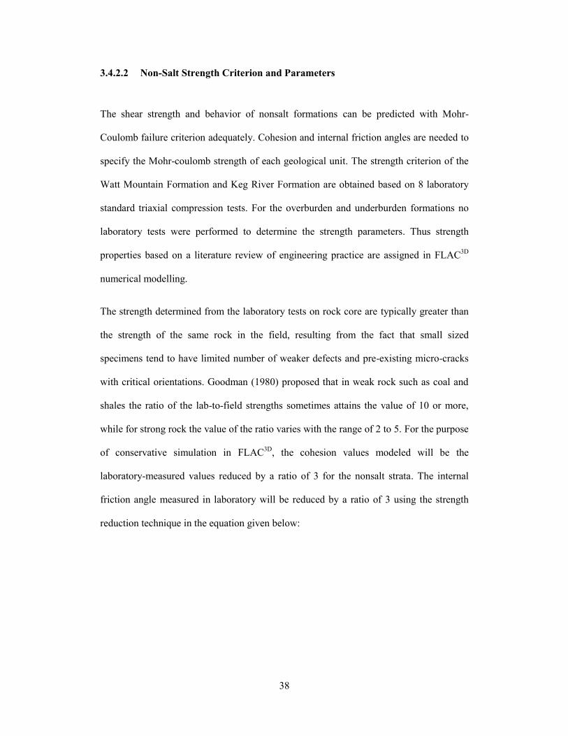
38
3.4.2.2 Non-Salt Strength Criterion and Parameters
The shear strength and behavior of nonsalt formations can be predicted with Mohr-
Coulomb failure criterion adequately. Cohesion and internal friction angles are needed to
specify the Mohr-coulomb strength of each geological unit. The strength criterion of the
Watt Mountain Formation and Keg River Formation are obtained based on 8 laboratory
standard triaxial compression tests. For the overburden and underburden formations no
laboratory tests were performed to determine the strength parameters. Thus strength
properties based on a literature review of engineering practice are assigned in FLAC3D
numerical modelling.
The strength determined from the laboratory tests on rock core are typically greater than
the strength of the same rock in the field, resulting from the fact that small sized
specimens tend to have limited number of weaker defects and pre-existing micro-cracks
with critical orientations. Goodman (1980) proposed that in weak rock such as coal and
shales the ratio of the lab-to-field strengths sometimes attains the value of 10 or more,
while for strong rock the value of the ratio varies with the range of 2 to 5. For the purpose
of conservative simulation in FLAC3D
, the cohesion values modeled will be the
laboratory-measured values reduced by a ratio of 3 for the nonsalt strata. The internal
friction angle measured in laboratory will be reduced by a ratio of 3 using the strength
reduction technique in the equation given below:
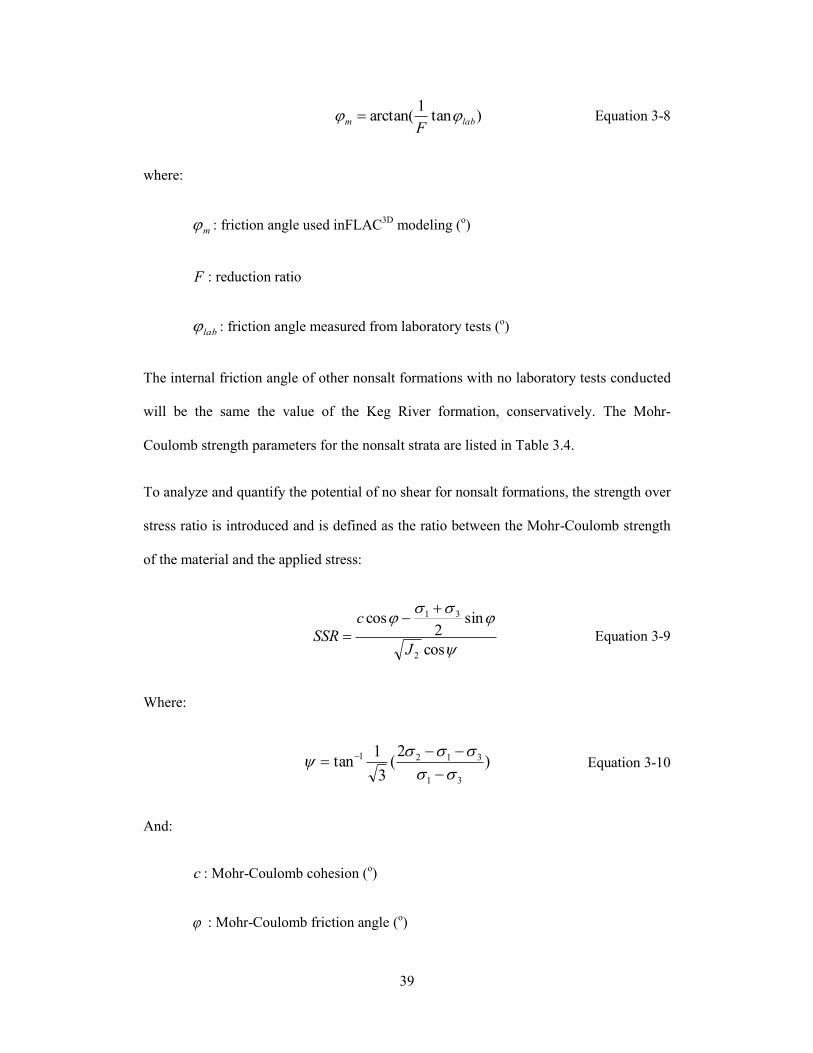
39
)tan1
arctan( labmF
Equation 3-8
where:
m : friction angle used inFLAC3D
modeling (o)
F : reduction ratio
lab : friction angle measured from laboratory tests (o)
The internal friction angle of other nonsalt formations with no laboratory tests conducted
will be the same the value of the Keg River formation, conservatively. The Mohr-
Coulomb strength parameters for the nonsalt strata are listed in Table 3.4.
To analyze and quantify the potential of no shear for nonsalt formations, the strength over
stress ratio is introduced and is defined as the ratio between the Mohr-Coulomb strength
of the material and the applied stress:
cos
sin2
cos
2
31
J
c
SSR
Equation 3-9
Where:
)2
(3
1tan
31
3121
Equation 3-10
And:
c : Mohr-Coulomb cohesion (o)
: Mohr-Coulomb friction angle (o)

40
Table 3.4 Mohr-Coulomb Strength Parameters of Non-Salt Formations
Nonsalt Unit
Laboratory
Friction Angle
(o)
Modeled
Friction Angle
(o)
Laboratory
Cohesion
(MPa)
Modeled
Cohesion
(MPa)
Upper Caprock 39.5 4
Middle Caprock 39.5 4
Lower Caprock 39.5 4
Watt Mountain 60 49 0.5 0.33
Keg River 51 39.5 6 4
Ernestina Lake 39.5 4
Underburden 39.5 4
Note: (lab) indicates the parameter value is determined on laboratory results, otherwise
the value is assumed from engineering experience.
3.5 In Situ Conditions
3.5.1 In Situ Lithostatic Stress Distribution
The initial in-situ lithostatic stress conditions are of importance to reasonably establish
the three dimensional finite difference models. The thickness of the geological units listed
in Table 3.1 and the bulk densities given in Table 3.3 were used to evaluate the initial
undisturbed lithostatic stress distributions of the salt site before solution mining of the
disposal caverns. The in situ stress distribution of salt formations is generally assumed to
be isotropic because salt creep will remove any stress difference after a long geological
time, and its ratio of vertical stress over horizontal stress is considered to be 1.0. As for
the nonsalt strata, which do not creep significantly during geological period, the
lithostatic stress state is generally taken as anisotropic. However, due to the lack of
geological history knowledge and site-specific measurements on nonsalt formations, the
anisotropic ratio cannot be assessed. In the FLAC3D
numerical simulations, the vertical
stress over horizontal stress ratios for nonsalt strata are estimated and compared by the
following equations respectively:

41
sin1k Equation 3-11
And:
)1/( k Equation 3-12
Where:
k : Vertical-horizontal stress ratio
: Friction angle (o)
: Poisson’s ratio
Table 3.5 provides the comparison of nonsalt anisotropic stress ratio value estimated from
the two different assessment methods, and shows a reasonably good agreement with each
other. As a conservative assumption, the modeled anisotropic stress ratio value in
FLAC3D
will be 0.5 for all the non-salt formations and 1 for all the salt strata.
Table 3.5 Anisotropic Stress Ratio of Geological Units used for Numerical Modeling
Geological Unit sin1k
)1/( k Modeled k
Upper Caprock 0.364 0.471 0.5
Middle Caprock 0.364 0.471 0.5
Lower Caprock 0.364 0.471 0.5
Watt Mountain 0.245 0.471 0.5
Prairie Evaporite - - 1
Keg River 0.364 0.389 0.5
Cold Lake - - 1
Ernestina Lake 0.364 0.429 0.5
Lotsberg - - 1
Underburden 0.364 0.429 0.5

42
3.5.2 Cavern Waste Disposal Stress Distribution
Salt cavern stability during the cavern creation process is important. To adequately
analyze the stress development around the cavern during solution mining and the
mechanical response of the disposal salt cavern after abandonment, it is critical to
determine an appropriate interpretation and representation of the cavern internal boundary
stresses used for numerical simulation in FLAC3D
.
Three different stages (Figure 3.6) during the cavern sump development were considered
for internal boundary stresses interpretation, that is (1) Development stage, before April
2006, the cavern is only filled with brine; (2) Sump operation stage, from April 2006 until
the current date, contributing to the solid waste injection and simultaneous solution
mining operation, the cavern is filled with unsaturated brine and oilfield disposal sands,
the composition of which might be brine, slurry, loose or medium sand or graded-
distributed dense sand; (3) Abandonment stage, once the cavern is fully filled with highly
consolidated waste sands and a small amount of saturated brine, the cavern will be
plugged and sealed for long-term abandonment.
In the cavern development stage, since the cavern is fully filled with brine, the cavern
internal pressure (IP) could be easily calculated as the summation of wellhead pressure
(WP) and hydraulic pressure (HP), where the equation ghHP is used. Wellhead
pressure could be read from the provided field data and an averaged value of 4MPa is
employed in the calculation. The schematic interpretation of internal stress calculation for
the initial stage is shown in Figure 3.7.
The schematic interpretation of internal stress calculation for abandonment stage is
shown in Figure 3.8. When considering the abandonment stage, the cavern internal
pressure becomes the total of wellhead pressure, hydraulic pressure and sands support

43
pressure (SSP). It is of critical importance to compute a reasonable estimate of the SSP
for simulation purposes. A thorough literature review was conducted to find previous
efforts on computing SSP but unfortunately, no related experimental researches was
found on SSP related to the disposal of sands in an abandonment cavern. Therefore, it has
been assumed that the behavior of the waste sands within the cavern will have similar
geotechnical properties as tailings and deposits for the tailing dam construction.
Rankine’s theory for estimating the passive earth pressure is adopted conveniently to
approximately calculate the resistance stress offered by the sands in the cavern due to
cavern creep after abandonment. The following equation is used:
hkhSSP wps '
Equation 3-13
and
)2/45(tan2 o
pk Equation 3-14
where:
'
s : Effective unit weight of the disposed sands in salt cavern
pk : Coefficient of passive earth pressure for waste sands
: Internal frictional angle of waste sands
Table 3.6 gives the range of total internal pressure if the internal material status in cavern
is varied from brine to dense sands. The unit weight and friction angle is estimated
roughly from literature on sand tailings for tailings dams. The lowest cavern internal
stress, which is due to the cavern filled only with brine is about 19.6MPa, while the
highest internal pressure could reach 25.6MPa if the cavern is filled with highly

44
consolidated disposal sands under which an extra pressure to the cavern is induced by the
sand’s support against the cavern wall.
Figure 3.6 Three Different Stages for Interpretation of Cavern Internal Boundary Stresses
Figure 3.7 Cavern Internal Boundary Stress Analysis for Development Stage
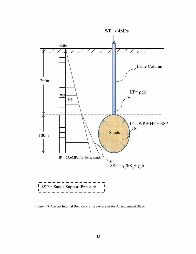
45
Figure 3.8 Cavern Internal Boundary Stress Analysis for Abandonment Stage
Brine Column
WP ≈ 4MPa
Sands
1200m
IP = WP + HP + SSP
HP= ρgh
4MPa
WP HP
IP = 25.6MPa for dense sands
100m
SSP = Sands Support Pressure
SSP = γs’hK
p+ γ
wh
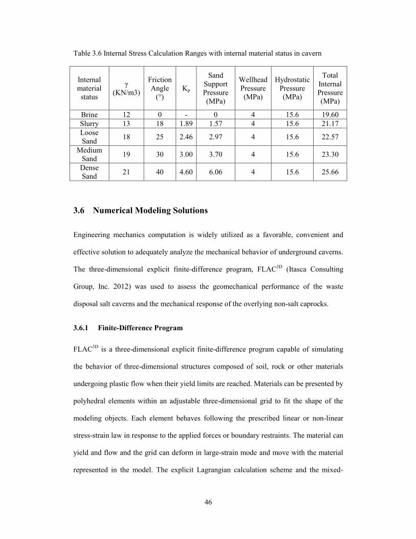
46
Table 3.6 Internal Stress Calculation Ranges with internal material status in cavern
Internal
material
status
γ
(KN/m3)
Friction
Angle
(°)
Kp
Sand
Support
Pressure
(MPa)
Wellhead
Pressure
(MPa)
Hydrostatic
Pressure
(MPa)
Total
Internal
Pressure
(MPa)
Brine 12 0 - 0 4 15.6 19.60
Slurry 13 18 1.89 1.57 4 15.6 21.17
Loose
Sand 18 25 2.46 2.97 4 15.6 22.57
Medium
Sand 19 30 3.00 3.70 4 15.6 23.30
Dense
Sand 21 40 4.60 6.06 4 15.6 25.66
3.6 Numerical Modeling Solutions
Engineering mechanics computation is widely utilized as a favorable, convenient and
effective solution to adequately analyze the mechanical behavior of underground caverns.
The three-dimensional explicit finite-difference program, FLAC3D
(Itasca Consulting
Group, Inc. 2012) was used to assess the geomechanical performance of the waste
disposal salt caverns and the mechanical response of the overlying non-salt caprocks.
3.6.1 Finite-Difference Program
FLAC3D
is a three-dimensional explicit finite-difference program capable of simulating
the behavior of three-dimensional structures composed of soil, rock or other materials
undergoing plastic flow when their yield limits are reached. Materials can be presented by
polyhedral elements within an adjustable three-dimensional grid to fit the shape of the
modeling objects. Each element behaves following the prescribed linear or non-linear
stress-strain law in response to the applied forces or boundary restraints. The material can
yield and flow and the grid can deform in large-strain mode and move with the material
represented in the model. The explicit Lagrangian calculation scheme and the mixed-

47
discretization zoning technique can ensure accurate modeled plastic collapse and flow in
FLAC3D
. FLAC3D
offers a wide range of capabilities to solve complex three-dimensional
problems especially in geomechanics, and embodies special numerical representations for
the mechanical response of geological materials. It has fifteen built-in material models,
including “null” model to simulate excavations, and plasticity models for brittle rock
behavior, and time-dependent volumetric yielding models to interpret the creep material
behavior. FLAC3D
also contains a powerful built-in programming language, FISH,
enabling the user to define new variables and functions to analyse specific simulation
needs.
The features and capabilities of FLAC3D
specially for the analysis in this thesis are (1)
ability of assigning arbitrary in-situ lithostatic stresses, (2) kinematic and traction
boundary conditions, (3) capability to simulate the sequential solution mining process and
sump operation process, (4) the built-in one-component power law to characterize the
creep behavior of salt units.
3.6.2 Three-Dimensional Finite Differential Model
A three dimensional finite difference model was developed in FLAC3D
(Version 5.0) to
evaluate the structural stability and integrity of the disposal salt caverns, the likelihood of
non-salt caprock failure and surface subsidence, interactions between adjacent caverns,
both during operation and after abandonment. Additionally, the numerical modeling
studies will be used to assess the casing integrity within and above the salt strata.
The performance criterion of the disposal salt caverns is related to the following
measurements:

48
The stress development around the caverns due to mining and operation of the
caverns was assessed to examine the evolution of the deviatoric stresses within
the geological units.
The structural stability and integrity of the salt units surrounding the solution-
mined caverns was evaluated with the value of dilation strength over the
deviatoric stress ratio DSR indicating the potential of dilation in salt strata.
Extensive salt dilation may lead to the cavern roof and/or wall spalling, and then
damage the casing seat. In addition, the microfractures developed within the salt
around the caverns may cause the leakage of the caverns, reducing the storage
capacity or even bring environmental issues at the site.
The integrity of the nonsalt overlying strata and the likelihood of failure were
assessed examining the factor of safety based on Mohr-Coulomb criterion with
respect to the shear failure within the formation. Shear failure of nonsalt caprock
may result in the wellbore and/or operational string failure, and reduce the cavern
integrity.
Surface subsidence resulting from the salt cavern closure is studied by evaluating
the vertical displacements in the numerical models. Large unexpected amount of
surface subsidence at the site may induce damage to the surface structures and
facilities and bring about economic loss.
The volume shrinkage and closure rate of the disposal salt cavern were estimated
during operation and after long-term abandonment. High level of cavern
shrinkage will directly reduce the storage volume of the waste disposal though
the cavern integrity may be raised by increasing internal pressure. More salt
caverns may need to be explored and operated for unplaced solid waste resulting
in additional project costs.
49
The integrity of the cemented casings was evaluated via checking the
accumulated casing strains. The casing will be dragged and stretched along the
casing axis, resulting from the cavern shrinkage and closure. Excessive strains
may lead to the tensile fracturing of the casing.
The axisymmetric FLAC3D
model developed extends vertically from the ground surface
to a depth of 1715 m, with 400 m thickness of underburden considered below the
Lotsberg salt formation to ensure the model boundary constraints, and the outer radius of
the model is 2000 m. These artificial truncations were selected to isolate the response of
the caverns against the boundary effects. The kinematic boundary conditions assigned to
the FLAC3D
models includes no normal displacement along the outer vertical boundaries,
and no vertical displacement on the bottom boundary. The upper surface of the model
was allowed to deform freely in the vertical and radial directions.
The cavern geometries are obtained based on the field sonar data tracking the cavern
development. Assumptions of cavern geometries are made to simplify the simulation
problems due to the irregular shape of 1-13 LTBG cavern. The geometry of modeled 1-13
LTBG cavern is assumed to be accumulated cylinders layer by layer and the maximum
radius and cavern height were scaled up to 72 m and 99 m respectively, ensuring the full
capacity of 750,000 m3 at abandonment. Considering the fact that the 8-13 LTBG cavern
is still in progress and the operation of two PRVP caverns is undetermined, the same
geometries will be used for these three caverns in numerical simulations. The two 1-13
cavern and two 8-13 caverns will be located symmetrically beside the centreline of the
FLAC3D
models.
To analyze the structural stability and cavern interaction between adjacent caverns, the
geomechanical assessment of disposal salt caverns is based on four types of cavern
50
combinations, there are (1) sole cavern case, only 1-13 LTBG cavern excavated
underground; (2) two horizontal caverns case, considering the existence of both 1-13
LTBG and 8-13 LTBG caverns, (3) two vertical caverns case, the abandonment of 1-13
LTBG cavern will be sequenced with the development of uphole 1-13 PRVP cavern and,
(4) four caverns case, full development of two downhole Lotsberg caverns and two
uphole Prairie Evaporite caverns. All the case conditions will be simulated based on
FLAC3D
models of same size and gridding method for the purpose of contrasting and
comparing the results of the simulations.
Moreover, the geomechanical response of the caverns will be studied based on two
diverse injection conditions for every cavern combination case, includes (1) the cavern(s)
will be abandoned with saturated brine only, then the internal cavern pressure will be
represented by an equivalent pressure applied as tractions normal to the surfaces of the
cavern walls, with a vertical pressure gradient of 0.011760 MPa/m and, (2) the cavern(s)
will be injected with normally consolidated dense sand waste and then be plugged and
abandoned, so the internal cavern pressure will be maintained with a vertical pressure
gradient of 0.072366 MPa/m for the Lotsberg and Prairie Evaporite caverns. This
gradient is only computed over the height of the cavern, not from the ground surface.
These two waste disposal conditions were selected as the lower and upper limit of the
cavern internal pressure respectively, and all the other waste injection conditions are
expected to lie within this range. Table 3.7 listed all the cases notated by various
combinations of cavern numbers and cavern injection conditions that will be studied in
FLAC3D
numerical modeling within this thesis. Among these listed cavern cases, the
conditions of caverns injected with brine and dense sands separately will be considered as
the worst and most unstable engineering operation problems, resulting from the
asymmetrical stress state along the centerline assigned on the model.

51
Table 3.7 Varied Cases Analyzed in FLAC3D
Numerical Modeling
Notation Case description
Sole Cavern
Case
1-13 LTBG brine 1-13 LTBG: brine
1-13 LTBG dense 1-13 LTBG: dense sands
Two
Horizontal
Caverns
1-13&8-13 LTBG brine-brine 1-13 LTBG: brine
8-13 LTBG: brine
1-13&8-13 LTBG dense-brine 1-13 LTBG: dense sands
8-13 LTBG: brine
1-13&8-13 LTBG dense-dense 1-13 LTBG: dense sands
8-13 LTBG: dense sands
Two Vertical
Caverns
1-13 LTBG&PRVP brine-brine 1-13 LTBG: brine
1-13 PRVP: brine
1-13 LTBG&PRVP dense-brine 1-13 LTBG: dense sands
1-13 PRVP: brine
1-13 LTBG&PRVP dense-dense 1-13 LTBG: dense sands
1-13 PRVP: dense sands
Four
Caverns
Case
1-13&8-13 LTBG&PRVP
brine-brine-brine-brine
1-13 LTBG: brine
8-13 LTBG: brine
1-13 PRVP: brine
8-13 PRVP: brine
1-13&8-13 LTBG&PRVP
dense-brine-brine-dense
1-13 LTBG: dense sands
8-13 LTBG: brine
1-13 PRVP: brine
8-13 PRVP: dense sands
1-13&8-13 LTBG&PRVP
dense-dense-brine-brine
1-13 LTBG: dense sands
8-13 LTBG: dense sands
1-13 PRVP: brine
8-13 PRVP: brine
1-13&8-13 LTBG&PRVP
dense-dense-dense-dense
1-13 LTBG: dense sands
8-13 LTBG: dense sands
1-13 PRVP: dense sands
8-13 PRVP: dense sands

52
4 SENSITIVITY ANALYSIS OF NUMERICAL MODELING
SOLUTIONS IN FLAC3D
4.1 Introduction
To study how well the FLAC3D
model predicts the cavern operations and abandonment
behavior, sensitivity studies are focused on various boundary conditions and potential
influencing parameters on the plugged and abandoned salt cavern(s) filled with brine.
This is a very critical stage, because it provides a degree of verification that the modeling
approach can reasonably represent the field behavior of the caverns. After the reliability
analysis the scenario will be repeated so that the operational and creep behavior of the
cavern(s) will be simulated under several different combinations of cavern locations.
Initialized with a reference model built for the typical sole cavern case (1-13 LTBG
brine), only one boundary value or influencing parameter is varied for each case study.
The investigated cases of cavern configurations considered in this chapter can be divided
into geometrical parameters, internal algorithm parameters (creep timestep) and
mechanical parameters (creep law parameters). After a series of sensitivity studies of
cavern cases, the most influencing or questionable parameters encountered during
numerical simulations will be examined and described in this chapter.
In Section 4.2, the reference models built for sensitivity studies are depicted in detail
from all engineering aspects. Section 4.3, 4.4 and 4.5 represents the results and outcomes
for geometrical, algorithm and geomechanical parameters respectively.
53
4.2 Reference Models in Sensitivity Analysis
The sensitivity studies of FLAC3D
models detailed in Section 4.3, 4.4 and 4.5 will be
based on and compared with the simulation results of the reference models described in
this section. The geometrical description and the mechanical parameters settings in the
reference models are all conformed to the actual salt cavern site conditions, for the
purpose of reasonably illustrating the effects of the varied parameters on the structural
stability or integrity of the caverns.
4.2.1 Geometrical description of the Reference Model
The assumed reference model is shaped mimicking the field solution-mined cavern with a
maximum radius of 72 m and a height of 99 m, giving the geometrical volume of about
750,000 m3. Cavern 1-13 LTBG is located between the depth of 1206 m and 1305 m in
the reference model, which starts from the ground and spreads downwards to the depth of
1715 m. The total length of the model is about 4000 m, with caverns symmetrically
arranged on both sides of the centerline of entire model.
The reference model is gridded as a Rad-Tunnel model. In FLAC3D
Rad-Tunnel gridding
is a way to grid the entire earth model as a radially graded mesh around parallelepiped-
shaped tunnel (Figure B.2 and Figure B.3 in Appendix B). The central parallelepiped
tunnel includes all target salt caverns inside. Moreover, to better observe the creep and
flow behavior of salt pillar and cavern walls, a gradually densified gridding method is
utilized from the earth model edge onto the cavern core area. In addition, the interface of
every two formations within the high influenced zone, and the salt pillar edge around the
salt cavern is very finely subdivided to detect any possible interface failure during the
simulation period. This Rad-tunnel model contains 838,198 grid points and 788,932
zones in total.

54
4.2.2 Rock Mechanical Material Parameters
The creep behavior in the reference model is described by the material law Power Law
with a set of parameters as shown in Table 3.3, Table 3.4 and Table 3.5. Real density of
each formation is utilized in the reference model. Initial horizontal stresses, which were
attempted to be reconciled with the in-situ conditions, are applied in the reference model.
4.2.3 Internal Algorithm Parameters
The related internal algorithm parameters used in the reference model are listed in Table
4.1. In FLAC3D
creep calculations; the creep time-step for every algorithm calculation
step is set to be 200 s throughout the 50 years creep after abandonment.
Table 4.1 Algorithm Parameters Setting in the Reference Models
Calculation
Year
Timestep
(second)
Minimum
timestep
(second)
Maximum
timestep
(second)
Real running
time (minutes)
0-2 year 200 400 4e4 100
2-5year 200 400 1e5 12
5-10year 200 400 2e5 15
10-20year 200 400 2.5e5 18
20-50year 200 400 4e5 32
4.3 Sensitivity Analysis of Geometrical Parameters in FLAC3D
Models
The geometrical parameters of most concern in the FLAC3D
numerical modeling of the
disposal salt caverns will include the model gridding method and the model outer
boundary size. To be specific, the pattern of the model gridding will influence the
accuracy of the computation and calculation results, resulting in unrevealed yielding or
failure behavior. The model boundary radius is determined artificially thus some degree
of unexpected boundary effects may be brought out and varied with the size variation.

55
The sensitivity analysis of the model gridding generation method and the boundary radius
influence will be discussed in Section 4.3.1 and 4.3.2, respectively.
4.3.1 Sensitivity Analysis of Gridding Generation Method
4.3.1.1 Methodology
Typically, grid generation is the first step when starting to construct and run a model for
numerical analysis. It is critical to create a relatively optimal gridding approach that can
sufficiently reveal the expected response and behavior, and making the model run
efficiently, particularly when up to 90 years of creep time calculations are involved in this
thesis.
In this section, the following case with varied gridding method will be presented in
comparison with the reference case. It adopts the Rad-Cylindrical gridding method,
which grids the earth model in FLAC3D
as a radially graded mesh around a cylindrical-
shaped tunnel. The central cylindrical tunnel is a zone with much more dense gridding
(see Appendix B), which will contain all the salt caverns inside. Rad-Cylindrical model
includes 1,380,729 grid points and 1,341,600 zones, which are two times of that of
reference model (Rad-cylindrical model). Other condition parameters will remain the
same as the reference model. Figure 4.1 and Figure 4.2 provides details of the 3D view
and the close view of caverns zone area of the Rad-Tunnel and Rad-Cylindrical Model
Respectively. As can be seen, in the reference model all the edges and boundaries which
are of most research interest become gradually more dense around the cavern(s), while in
Rad-Cylindrical model the salt zones are subdivided uniformly and are assigned the same
importance. The cavern injection condition considered in this gridding sensitivity study
will be the saturated brine case only, which is represented by a vertical pressure gradient
of 0.011760 MPa/m.

56
4.3.1.2 Results and Conclusions
The simulation results comparison is based on both single cavern case (1-13 LTBG brine)
and two Lotsberg caverns (1-13&8-13 LTBG dense-brine) case condition. Figure 4.3
illustrates the contour of DSR value with respect to the dilation in the salt units
surrounding cavern 1-13 LTBG for two different gridding methods following 4 months
after the abandonment of disposal caverns. It can be shown that the distributions of the
DSR value are almost the same for the two gridded models, with an increasing DSR value
with increasing distance away from the cavern wall. However, the minimum DSR value
around the salt cavern in the reference is 1.37, which is much less than the value of 1.73
for the Rad-Cylindrical model. Thus the conclusion can be made that the Rad-tunnel
gridding has a much better ability of detecting the dilation or tensile failure of the salt
strata around the mined caverns than the Rad-Cylindrical gridding.
Table 4.2 summarises the results of sensitivity measurement values during 50 years creep
simulation in Rad-Cylindrical and Rad-Tunnel models for the two studied cases in
FLAC3D
. It can be seen that the minimum SSR values with respect to the failure potential
of the overlying nonsalt strata for two gridding method are equal to each other, which
indicates that the gridding methods have little impact on the shear failure of the non-salt
units. Moreover, the Rad-Tunnel models could predict slightly more deformation of the
geological formations, including surface subsidence and the theoretical casing strains.
Additionally, the reference model can save as much as 33% run-time over the
calculations under the same case.
In conclusion, Rad-Tunnel Gridding method will be utilized in the following numerical
simulation process due to its higher sensitivity to the salt dilation and formation
deformation behavior and it is more efficient in calculations.

57
Table 4.2 Comparison of 50-year Abandonment Behavior Results Simulated in Rad-
Cylindrical and Rad-Tunnel Models
Measurements
1-13 LTBG 1-13&8-13 LTBG
Rad-
Tunnel
Rad-
Cylindrical
Rad-
Tunnel
Rad-
Cylindrical
Surface Subsidence
(mm) 9.4 8 16.4 14.8
Maximum Casing Strain 0.000302 0.000262 0.000322 0.000270
Minimum SSR 3.27 3.28 2.47 2.46
Calculation Time 2.6h 4h 3h 4.5h

58
3D View of Rad-Tunnel Model
Pre-Solutioning
Post-Solutioning
Figure 4.1 Detailed Gridding View of Rad-Tunnel Model (Reference Model)
1-13 LTBG 8-13 LTBG

59
3D View of Rad-Cylindrical Model
Pre-Solutioning
Post-Solutioning
Figure 4.2 Detailed Gridding View of Rad-Cylindrical Model
1-13 LTBG 8-13 LTBG

60
Rad-Tunnel Model (Reference Model) (Time = 4 months)
Legend of DSR
Value
(-)
Rad-Cylindrical Model (Time = 4 months)
Figure 4.3 Predicted DSR Value in the Salt Strata Surrounding Cavern 1-13 LTBG
Lotsberg
Minimum DSR = 1.37
Lotsberg
Minimum DSR = 1.73

61
4.3.2 Sensitivity Analysis of Boundary Size
4.3.2.1 Methodology
When modeling infinite bodies or very large bodies, it may not be possible to cover the
whole body with zones, due to constraints on memory and computer time. Artificial
boundaries are placed sufficiently far away from the area of interest such that the
behavior in that area is not affected.
To conduct the boundary effect analysis in FLAC3D
, several boundary sizes different
from the value of 2000 m in the reference model are chosen to run the simulation. It is
expected to find a relatively reasonable and optimal boundary value at which the
subsidence of the model edge is almost zero and can be ignored so that the boundary
effect can be eliminated.
The reference model based on the condition of two Lotsberg caverns (1-13&8-13 LTBG
dense-brine) is chosen in the boundary sensitivity analysis and simulated under the
injection condition of 1-13 LTBG cavern with dense sands and 8-13 LTBG cavern with
saturated brine, since it is less stable as compared to other injection conditions. Boundary
sizes tested in the following section include 1000 m, 1200 m, 1500 m, 2500 m and 3000
m respectively, which presents the outer radius of the entire model.
4.3.2.2 Results and Conclusions
Figure 4.4 presents the 50-year abandonment surface subsidence plot for each tested
boundary size, and it can be seen that the subsidence at the edge of the model is
decreasing as the boundary size increases. When the boundary size is below 1200 m, the
boundary effect is so significant that the vertical displacement at the model edge is almost
50% of the maximum surface subsidence. This boundary effect will be largely reduced

62
when the size value increases to 2000 m, where edge settlement is calculated as only 8%
of the maximum displacement. The central subsidence of the model almost remains the
same, fluctuating within 2 mm. Table 4.3 provide additional information of the minimum
DSR values for the Lotsberg salt formation and minimum SSR values for the non-salt
Ernestina Lake formation and it is clear that even the smallest boundary constraint of
1000 m will not affect the salt dilation and non-salt shear failure behavior. In conclusion,
the reference model with 2000 m boundary size value can predict the model behavior
with negligible boundary effect.
Figure 4.4 Comparison of 50-year Surface Subsidence for Varied Boundary Sizes
-20
-18
-16
-14
-12
-10
-8
-6
-4
-2
0
0 500 1000 1500 2000 2500 3000
Surf
ace
Su
bsi
de
nce
(m
m)
Radial Distance (m) 1-13&8-13 LTBG dense-brine case
3000m Boundary Size
2500m Boundary Size
2000m Boundary Size
1500m Boundary Size
1200m Boundary Size
1000m Boundary Size

63
Figure 4.4 Edge Subsidence Varied with Boundary Size
Table 4.3 Summarized 50-year Measurements for Varied Boundary Sizes
Measurements Boundary Size
Subsidence (mm) 1000m 1200m 1500m 2000m 2500m 3000m
Centre point 18.61 18.15 17.58 16.42 16.69 16.48
Boundary point 10.26 7.28 3.74 1.29 0.47 0.01
Minimum DSR 2.30 2.30 2.30 2.30 2.30 2.30
Minimum SSR 2.486 2.486 2.485 2.485 2.485 2.484
4.4 Sensitivity Analysis of Creep Timestep Parameter
4.4.1 Methodology
The first and most critical parameter analyzed for creep computation calculations in
numerical modeling is the creep timestep parameter, because the major difference
between creep and other constitutive models in FLAC3D
is the concept of problem time in
10.26
7.28
3.74
1.29 0.47 0.24
y = 69.524e-0.002x R² = 0.9945
0
2
4
6
8
10
12
14
16
18
20
0 500 1000 1500 2000 2500 3000 3500
Sub
sid
en
ce (
mm
)
Boundary Size (m)
Edge SubsidenceMaximum Subsidence
64
the simulation. The creep constitutive law used for the rock type involves timestep in
their calculation equations, which may affect the response because the timestep here
represents the real time rather than an artificial quantity used only for contributing to step
to a steady-state condition.
In a creep simulation, the value of creep timestep needs to be varied in a range to ensure
the time-dependent stress changes produced by the creep constitutive law are not larger
than the strain-dependent stress changes, preventing large out-of-balance forces. In
FLAC3D
a rough estimation equation for the maximum creep timestep for numerical
accuracy is suggested and expressed as the ratio of the material viscosity to the shear
modulus,
Gt cr /max Equation 4-1
For the power law the viscosity can be evaluated as the ratio of the stress magnitude, ,
to the creep rate, cr . Using equation 4.1 the maximum creep timestep is rewritten as:
AGt ncr /1
max
Equation 4-2
The stress magnitude, , also known as the von Mises stress invariant, can be determined
from the initial stress state before the creep process begins.
FLAC3D
also recommends that a creep analysis could begin with an initial creep timestep
approximately two to three orders of magnitude smaller than the calculated crtmax using
the estimation equation above. Moreover, typically a gradually increased or decreased
timestep can be utilized to obtain a good performance efficiently.
In the comparison model for timestep sensitivity studies, the two horizontal caverns (1-
13&8-13 LTBG dense-brine) case are researched and analyzed. Table 4.4 shows the
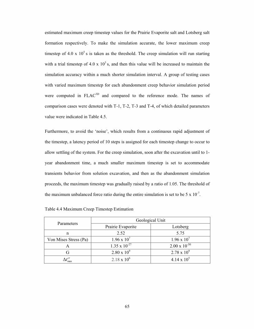
65
estimated maximum creep timestep values for the Prairie Evaporite salt and Lotsberg salt
formation respectively. To make the simulation accurate, the lower maximum creep
timestep of 4.0 x 10⁵
s is taken as the threshold. The creep simulation will run starting
with a trial timestep of 4.0 x 10³
s, and then this value will be increased to maintain the
simulation accuracy within a much shorter simulation interval. A group of testing cases
with varied maximum timestep for each abandonment creep behavior simulation period
were computed in FLAC3D
and compared to the reference mode. The names of
comparison cases were denoted with T-1, T-2, T-3 and T-4, of which detailed parameters
value were indicated in Table 4.5.
Furthermore, to avoid the ‘noise’, which results from a continuous rapid adjustment of
the timestep, a latency period of 10 steps is assigned for each timestep change to occur to
allow settling of the system. For the creep simulation, soon after the excavation until to 1-
year abandonment time, a much smaller maximum timestep is set to accommodate
transients behavior from solution excavation, and then as the abandonment simulation
proceeds, the maximum timestep was gradually raised by a ratio of 1.05. The threshold of
the maximum unbalanced force ratio during the entire simulation is set to be 5 x 10⁻⁷
.
Table 4.4 Maximum Creep Timestep Estimation
Parameters Geological Unit
Prairie Evaporite Lotsberg
n 2.52 5.75
Von Mises Stress (Pa) 1.96 x 10⁷ 1.96 x 10
7
A 1.35 x 10⁻²⁷
2.00 x 10-50
G 2.80 x 10⁹ 2.78 x 10
9
crtmax
2.18 x 10⁶ 4.14 x 10
5

66
Table 4.5 Maximum Timestep for Variation Comparison Cases
Maximum Timestep (s)
Creep Time Reference case T-1 T-2 T-3 T-4
0 - 1year 4.0 x 10⁴ 4.0 x 10
3 4.0 x 10
4 1.0 x 10
5 3.0 x 10
5
1 - 2 year 4.0 x 10⁴ 4.0 x 10
3 4.0 x 10
4 2.0 x 10
5 3.0 x 10
5
2 - 5 year 1.0 x 10⁵ 4.0 x 10
3 4.0 x 10
4 3.0 x 10
5 3.0 x 10
5
5 - 10 year 2.0 x 10⁵ 4.0 x 10
3 4.0 x 10
4 4.0 x 10
5 3.0 x 10
5
10 - 20 year 2. 5 x 10⁵ 4.0 x 10
3 4.0 x 10
4 4.0 x 10
5 3.0 x 10
5
20 - 50 year 4.0 x 10⁵ 4.0 x 10
3 4.0 x 10
4 4.0 x 10
5 3.0 x 10
5
4.4.2 Results and Conclusions
As shown in Table 4.5, Case T-1 uses the most conservative maximum timestep two
orders of magnitude smaller than the estimated maximum timestep, so that it could
theoretically generate the most accurate simulation results. It can be seen in Table 4.6 that
the reference model and the T-2 model produce almost the same surface subsidence and
maximum vertical displacement as the T-1 model and it is also more sensitive to the salt
dilation behavior and shear, failure which may occur during the simulations. Among
these three tests, the reference model shows the obvious advantage of saving the model
simulation time significantly, consuming approximately 88% less runtime than that of the
T-1 model. The runtime is a critical factor for this thesis as many different simulations
were run to reveal the cavern creep behavior. However, the T-3 and T-4 models reveal
zero surface subsidence for the 1-year or 2-year abandonment time, and gives much
higher cavern vertical displacement, even the runtime is only 1 to 1.5 hours. In
conclusion, the creep timestep parameters set for the reference model could efficiently
develop relatively higher calculation accuracy thus they will be repeatedly used in the
Chapter 5.

67
Table 4.6 Results of Creep Timestep Sensitivity Analysis
Creep Year Reference
case T-1 T-2 T-3 T-4
Surface Subsidence (mm)
1 4.25 4.25 4.25 0 0
2 5.5 5.5 5.5 2.6 0
5 6.2 6.3 6.6 12 2.8
10 8 8 8 12 10
20 10 10 11 12 10
50 16 16 16 16 18
Maximum Z-displacement (mm)
1 264 264 264 327 400
2 308 308 308 291 625
5 388 388 388 522 615
10 472 471 471 544 694
20 585 587 590 655 747
50 800 802 806 848 917
Minimum DSR
4 month 1.37 1.37 1.37 1.27 1.26
Minimum SSR
4 month 3.22 3.20 2.93 2.50 2.45
Model Total Running Time (hours)
1 – 50 y 3 25 5 1 1.5
4.5 Sensitivity Analysis of Mechanical Parameters
The parameters of the one-component Power law used to simulate the strength and
deformation mechanisms of the salt formations require sensitivity analyses to show how
the simulation results will be influenced with their changes. The test cases in this section
are all based on the single 1-13 Lotsberg cavern case.
4.5.1 Elastic Properties
4.5.1.1 Methodology
The elastic properties are important in predicting deformation behavior of the salt caverns.
However, the elastic properties determined from both laboratory tests or estimated from
wireline logs in filed can vary from 6 GPa to 20 GPa for salt strata. Thus some degree of

68
emphasis needs to be put onto how the elastic properties, particularly the Young’s
modulus, will influence the simulation results.
The Young’s modulus used in the reference model is 7 GPa for the Lotsberg Formation.
In the sensitivity studies in this section, only the elastic modulus for the Lotsberg salt will
be changed for each test case. Young’s modulus was varied as follows: 6 GPa, 10 GPa,
15 GPa and 20 GPa.
4.5.1.2 Results and Conclusions
Table 4.7 demonstrates the sensitivity results of Young’s modulus. It shows that
increasing Young’s modulus will result in some amount of declining surface subsidence,
which is primarily the result of a decrease in the closure rate of the caverns. The value of
Young’s modulus used in the reference case is quite conservative as for the shrinkage
responses of the disposal salt caverns. However, the varied Young’s modulus has
negligible impact on the dilation of the salt and the shear failure of the nonsalt strata.
Table 4.7 Sensitivity Analysis Results of Young’s Modulus, Time = 5 years
Young’s
Modulus
(GPa)
Bulk
Modulus
(GPa)
Shear
Modulus
(GPa)
Maximum
Surface
Subsidence (mm)
Minimum
DSR
6 4.17 2.38 3.7 1.87
7 4.86 2.78 3.5 1.88
10 6.94 3.97 3.3 1.9
15 10.42 5.95 3.1 1.91
20 13.89 7.94 3 1.93

69
Figure 4.5 Sensitivity Plot of Young's Modulus
4.5.2 Power Law Parameters
4.5.2.1 Methodology
The parameters, A and n are used to describe one-component Power law for salt strata.
Since there is a link between these two parameters, three ways to study the sensitivity of
power law parameters are evaluated in this section. Firstly, the n parameter was held
constant and only changes in the value of A by order of magnitude were implemented.
Secondly, the A parameter was held constant and the n value was varied by 0.25 for every
step. Lastly, both A and n were varied simultaneously to obtain the same simulation
results as the default models. In the reference models for sensitivity analysis, A is set to
be 2 x 10-50
, and n is set to be 5.75, which are derived from laboratory creep tests.
y = 577.94x-0.22 R² = 0.9847
0
1
2
3
4
5
6
7
8
9
10
0
50
100
150
200
250
300
350
400
450
0 5 10 15 20 25
Min
imu
m D
SR o
r SS
R
Cav
ern
Max
imu
m z
dis
p (
mm
)
Young's Modulus (GPa)
1-13 LTBG brine-case
Cavern Maximum zdisp
DSR
SSR

70
4.5.2.2 Results and Conclusions
Table 4.8 and Table 4.9 contain detailed results of sensitivity analysis of A and n
parameter respectively. The deformation behavior of the model is largely influenced by
the A and n value respectively because they dominate the flow rule for the salt creep. The
degree of marginal effect of A is dramatically enlarged with more positive deviation from
A value in the reference model, which is also the case for n parameter. The maximum
surface subsidence of the model will even increase to about six times that of the reference
results when the A value is increased by two orders of magnitude. Once any parameter (A
or n) of the power law increases, the creep rate of the salt will increase and then the salt
surrounding the disposal caverns will maintain a stable state at a higher rate, thus the DSR
value following 5-year creep simulation will also rise as shown in Figure 4.7 and 4.8,
indicating more stability of the salt strata. However, the shear failure behavior of the non-
salt overlying formations will not be influenced by the change of the power law
parameters. Figure 4.9 demonstrates the contour of A and n representing the same
deformation results as the reference model. This evidently shows that there is a strong
link between the A and n parameter and for this project, every one order of magnitude’s
increase of A with every 0.15 decreases in n parameter will keep the simulation results
the same. In conclusion, the decision of A and n parameters of power law is of critical
importance on the study of the dilation response of salt units and the deformation
behavior of the model in FLAC3D
numerical simulations.
Table 4.8 Sensitivity Analysis Results of A parameter for Power Law, Time = 5 years
A n Surface subsidence (mm) Minimum DSR Minimum SSR
2.00E-52 5.75 1.5 1.14 3.23
2.00E-51 5.75 2 1.45 3.21
2.00E-50 5.75 3.5 1.88 3.17
2.00E-49 5.75 8.2 2.4 3.27
2.00E-48 5.75 18 2.96 3.52

71
Table 4.9 Sensitivity Analysis Results of n parameter for Power Law, Time = 5 years
A n Surface subsidence (mm) Minimum DSR Minimum SSR
2.00E-50 5.25 1.2 0.8 1.91
2.00E-50 5.5 1.6 1.2 3.21
2.00E-50 5.75 3.5 1.88 3.17
2.00E-50 6 16 2.78 3.39
2.00E-50 6.25 N/A N/A N/A
Notes: N/A indicates calculation overflow in FLAC3D
.
Table 4.10 Sensitivity Analysis Results of A & n parameter for Power Law, Time = 5
years
A n Surface subsidence (mm) Minimum DSR Minimum SSR
2.00E-49 5.6 3.42 1.86 3.17
2.00E-50 5.75 3.5 1.88 3.17
2.00E-51 5.9 3.5 1.9 3.17
2.00E-52 6.05 3.6 1.92 3.17
Figure 4.6 Sensitivity Plot of A parameter for Power Law, Time = 5 years
y = 3E+14x0.2771 R² = 0.9686
y = 298769x0.1048 R² = 0.9988
0
0.5
1
1.5
2
2.5
3
3.5
4
4.5
5
0
2
4
6
8
10
12
14
16
18
20
1E-52 1E-51 1E-50 1E-49 1E-48 1E-47
Min
imu
m D
SR/S
SR V
alu
e
MA
xim
um
Su
rfac
e S
ub
sid
en
ce (
mm
)
A Parameter
1-13 LTBG brine-case
Maximum Surface Subsidence
DSR
SSR

72
Figure 4.7 Sensitivity Plot of n parameter for Power Law, Time = 5 years
Figure 4.8 Contour of A and n representing same results as Reference Model
y = 2E-14x19.089 R² = 0.8934
y = 1E-07x9.4028 R² = 0.9992
0
0.5
1
1.5
2
2.5
3
3.5
4
4.5
5
0
2
4
6
8
10
12
14
16
18
20
5.2 5.4 5.6 5.8 6 6.2
Min
imu
m D
SR/S
SR V
alu
e
Max
imu
m S
urf
ace
Su
bsi
de
nce
(m
m)
n Parameter
1-13 LTBG brine-case
Maximum Surface Subsidence
DSR
SSR
y = 1.5976x-0.011 R² = 0.9999
0
1
2
3
4
5
6
7
8
9
10
5.55
5.6
5.65
5.7
5.75
5.8
5.85
5.9
5.95
6
6.05
6.1
1E-52 1E-51 1E-50 1E-49 1E-48
Min
imu
m D
SR/S
SR V
alu
e
Co
resp
on
din
g n
Val
ue
A Parameter
1-13 LTBG brine-case
n valueDSRSSR

73
4.6 Summary and Conclusions
This chapter has described a series of sensitivity analyses of some critical geometrical
parameters (gridding method and boundary effects), algorithmic parameters (creep
timestep), elastic parameters (Young’s modulus) and power law parameters (A and n) in
detail for the disposal salt caverns. The reference model for the purpose of comparison
was introduced from the point of potential sensitive factors.
The Rad-Tunnel gridding pattern behaves more sensitive to the dilation behavior of the
salt strata, more fairly and conservatively presenting the potential of loss of stability of
the disposal salt caverns than the Rad-Cylindrical gridding method. Also, it gives slightly
more deformation in the modeled geological units and save approximately one third of
the computation time in FLAC3D
simulations.
The size of the outer boundaries can bring a significant influence on the surface
subsidence prediction of the model, especially at the edge point. When the outer radius
of the model increase to the value of 2000 m, the marginal subsidence of the surface area
reduced to almost zero and the maximum subsidence remains in the reasonable range.
Fortunately, the boundary size has little effects on the salt dilation and overlying nonsalt
shear failure behavior around the disposal caverns.
A good determination of the creep timestep embedded in FLAC3D
simulation program
can benefit the numerical simulation not only in the terms of fairly reasonable results
output but also saving massive calculation time. The range of creep timestep predicting
adequate deformations and salt dilation or non-salt failure potential will be used in the
following FLAC3D
numerical modeling based on different cavern cases.

74
The research of elastic parameters shows that the value of Young’s modulus has limited
influence on the model deformation and as well as the salt dilation and nonsalt shear
failure behavior predicted in the FLAC3D
simulations.
It was shown that the power law parameters could influence the model deformation
significantly, along with the dilation behavior of the surrounding salt units of the disposal
caverns. Since there existed a high degree of uncertainty in the power law parameters
estimation from the laboratory tests, the simulated structural stability and the integrity of
the disposal salt caverns in this thesis could be used as a referenced geomechanical
assessment.
75
5 LONG-TERM ABANDONMENT BEHAVIOR
SIMULATION OF WASTE DISPOSAL SALT CAVERNS
5.1 Introduction
The structural stability and creep performance during the solution-mining process and
after abandonment of the disposal salt caverns is conservatively evaluated using three-
dimensional finite difference model in FLAC3D
. Various combinations of salt cavern
conditions were considered in numerical simulations. The geomechanical assessments are
related to (1) salt cavern structural stability and likelihood of failure of salt and their
caprocks during the operational and abandonment period, (2) cavern creep closure
behavior over time, (3) theoretical casing strains predictions, (4) stress development
around the salt caverns, (5) surface subsidence development.
Simulations of the cavern solution mining process are represented as instantaneous
excavation of the entire salt cavern(s) and sequential excavations of cavern layers
respectively, along with the corresponding modeling results being compared and
analyzed. The cavern(s) will be maintained at a constant saturated brine pressure gradient
of 0.011760 MPa/m representing the brine injection condition, or at a vertical constant
pressure gradient of 0.072366 MPa/m presenting the dense sand disposal condition. Each
type of excavation model will be simulated with another 50-year creep period following
the full development of all salt caverns.
The long-term abandonment simulation behavior of the sole cavern case, i.e. only 1-13
LTBG cavern, will be discussed in Section 5.2 based on both instantaneous excavations
and sequential excavations respectively. The brine injection status is considered for both

76
solutions. Additionally, 1-13 LTBG cavern excavated sequentially will be simulated with
the disposal of the injected dense sands.
The same analysis scenario will be performed on the long-term abandonment creep
behavior of two horizontally adjacent Lotsberg caverns in Section 5.3. The simulation
comparison of instantaneous and sequential excavations will be evaluated with Cavern 1-
13 LTBG containing dense sands at abandonment and Cavern 8-13 LTBG injected with
saturated brine. Then the two horizontally adjacent Lotsberg caverns will be modeled
under both caverns with brine as well as both caverns with disposal sands in FLAC3D
numerical modeling studies.
The abandonment performance of the two vertical adjacent caverns (1-13 LTBG&PRVP)
was simulated considering only sequential excavation processes. The caverns were
assumed to be abandoned at three different injection times, including (1) both caverns
with brine, (2) the lower cavern with dense sands while the upper cavern with brine, (3)
both of the caverns with dense disposal waste. The detailed descriptions of three-
dimensional finite difference models and discussion are presented in Section 5.4.
The full sequential development of four caverns in both Lotsberg and Prairie Evaporite
formations were simulated in FLAC3D
numerical modeling to study the operational and
abandonment performance of each cavern and the interactions occur between 1-13 and
8-13 well salt caverns. Various cavern internal pressure conditions, including three
symmetrical and one asymmetrical injection scenario are analyzed, compared and
discussed in Section 5.5.

77
5.2 Long-term Abandonment Behavior Simulation of Single Cavern
5.2.1 Long-term Abandonment Behavior Considering Instantaneous Excavation
In the three dimensional finite difference modeling, instantaneous excavation of 1-13
LTBG cavern is considered prior to the abandonment of waste disposal salt cavern. At the
start of the abandonment creep behavior simulation, the displacement and velocity of grid
points of FLAC3D
model was reset to be zero. Cavern 1-13 LTBG was held at a saturated
brine pressure gradient of 0.011760 MPa/m throughout the 50 years creep simulation.
The internal cavern pressure is assumed to be constant over time. The total creep
simulation time is 50 years.
5.2.2 Long-term Abandonment Behavior Considering Sequential Excavations
Sequential excavations can reasonably simulate the field operational solution mining
processes of the disposal caverns at the site. According to the field sonar data tracking the
cavern development progress, the sequential excavations are arranged to start from the
beginning of 2006 and will be finished by the end of 2015, assuming a 10-year solution
mining schedule. Following the full development of the salt cavern, the 1-13 LTBG
cavern was planned to fill with saturated brine or dense sands and abandoned
permanently. Table C.1, C.2 and C.3 (Appendix C) detail the 1-13 LTBG cavern
solution-mined process and abandonment schedule in FLAC3D
simulation. In the first 10-
year mining period, the cavern simulation will undergo creep for a whole year after each
immediate excavation at the beginning of the year, and then in the start of 2016 the
abandonment creep simulation proceeds and will model for another 50 years to assess the
geomechanical behavior of the salt caverns. Thus the salt caverns will run 60 years in
total for creep simulations. Figure 5.1 depicts the three-dimensional finite difference
models used for Cavern 1-13 LTBG, and the detailed cavern geometry.
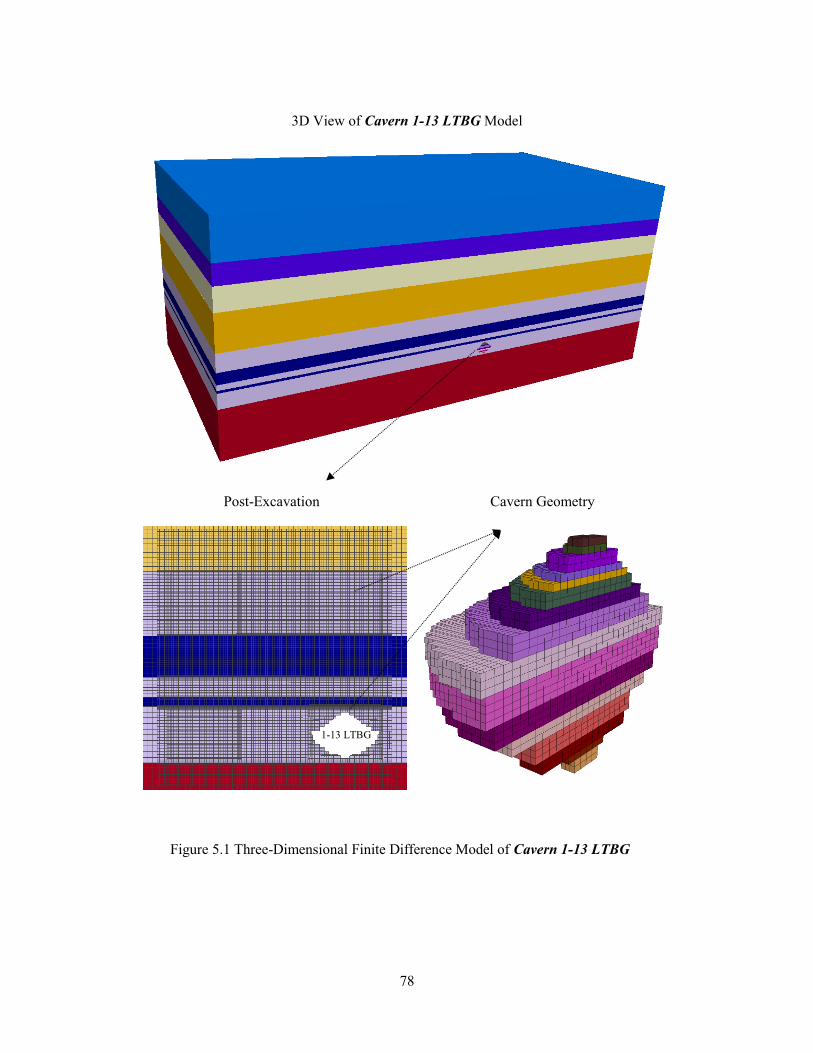
78
3D View of Cavern 1-13 LTBG Model
Post-Excavation
Cavern Geometry
Figure 5.1 Three-Dimensional Finite Difference Model of Cavern 1-13 LTBG
1-13 LTBG

79
5.2.3 Results and Conclusions
Table 5.1 summarize the observed deformation simulation results and the DSR value with
respect to salt dilation potential and the SSR value representing the shear failure potential
of non-salt overlying strata. It indicates that the sequential excavation modeling predicts
slightly more deformation than instantaneous excavations at number of years of
abandonment, due to sequential excavations allowing the cavern to creep over a longer
period of time and generate more deformation after each excavation procedure. However,
instantaneous simulations predict cavern closure ratio at the end of simulation
approximately two times of the sequential excavation simulations. Additionally, the
predicted DSR and SSR values as a function of abandonment time are given in Figure 5.2.
As shown, during the first few years of abandonment, the DSR value under the sequential
excavations is apparently higher than the value under instantaneous excavations. This is
because that the 10-year solution mining period time considered prior to the abandonment
for sequential condition, results in the reduced deviatoric stresses of the salt surrounding
the cavern as it creeps and the DSR value will grow above the instantaneous case. The
value of DSR immediately following the final instantaneous excavation is 0.825, which
means the salt units around the cavern have dilated and tensile failure may be initialized
within the salt. However, the ultimate DSR values after 50 years abandonment for both
excavation conditions are similar, indicating that the instantaneous excavation methods
can predict the final abandonment salt stability adequately as the sequential excavations.
The SSR values do not vary much during the abandonment modeling and they are
identical for both excavation simulations. Thus the excavation simulation method has
little impact on the shear failure behavior of the nonsalt units. In conclusion, the
instantaneous excavations would result in salt dilation prediction at the end of full
excavations but it is not the case in sequential excavations. From a view of long-term

80
abandonment behavior, both excavations can predict the similar deformation behavior
and the structural stability performance. However, the instantaneous excavations
simulation will overestimate the cavern volume loss significantly.
More simulations were run for the case of the 1-13 LTBG sequentially solution mined
and filled with dense waste sands at abandonment, and compared with the corresponding
brine case. The structural stability and integrity of the salt cavern is examined with
respect to the potential dilation or tensile failure along the cavern walls and the shear
failure of nonsalt caprock formations. When the cavern contents are replaced with
saturated brine, the loads that supported the cavern change. The deviatoric stress in the
surrounding strata changes and when it exceeds the strength of the formation, salt dilation
or nonsalt shear failure will happen. Figure 5.3, 5.4 and 5.5 illustrate the deviatoric
stresses distribution, DSR value and SSR value surrounding the 1-13 LTBG cavern under
both brine and dense sands injection respectively. Figure 5.6 plots the DSR and SSR value
change during cavern development and after abandonment. As shown, following the final
sequential excavation, the deviatoric stresses of the salt units surrounding the cavern
increased immediately and the stress change resulted in the redistribution of the
maximum deviatoric stress. As the creep continues with abandonment, salt deviatoric
stresses decreases thus the DSR value increases, which indicates that the potential of salt
dilation diminishes over time. All the DSR values during the simulation time for 1-13
LTBG brine and dense sands case are greater than 1.0, so if no salt dilation is expected to
occur during the cavern development period, then the integrity of the salt cavern will not
be affected by the salt dilation within permanent abandonment. Additionally, the potential
of salt dilation is largely diminished by the solid waste sands injection. Since the initial
lithostatic anisotropic ratio of 0.5 considered for the overlying nonsalt Ernestina Lake
formation in the simulation, the deviatoric stress above the cavern roof in the nonsalt
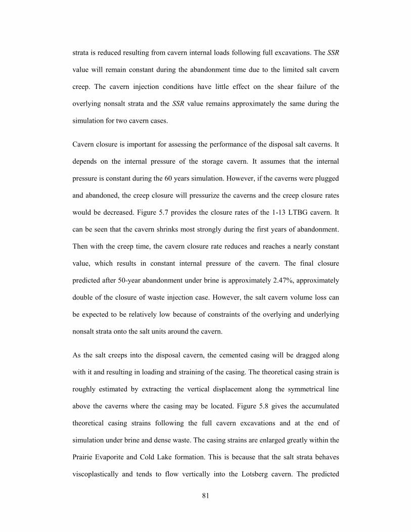
81
strata is reduced resulting from cavern internal loads following full excavations. The SSR
value will remain constant during the abandonment time due to the limited salt cavern
creep. The cavern injection conditions have little effect on the shear failure of the
overlying nonsalt strata and the SSR value remains approximately the same during the
simulation for two cavern cases.
Cavern closure is important for assessing the performance of the disposal salt caverns. It
depends on the internal pressure of the storage cavern. It assumes that the internal
pressure is constant during the 60 years simulation. However, if the caverns were plugged
and abandoned, the creep closure will pressurize the caverns and the creep closure rates
would be decreased. Figure 5.7 provides the closure rates of the 1-13 LTBG cavern. It
can be seen that the cavern shrinks most strongly during the first years of abandonment.
Then with the creep time, the cavern closure rate reduces and reaches a nearly constant
value, which results in constant internal pressure of the cavern. The final closure
predicted after 50-year abandonment under brine is approximately 2.47%, approximately
double of the closure of waste injection case. However, the salt cavern volume loss can
be expected to be relatively low because of constraints of the overlying and underlying
nonsalt strata onto the salt units around the cavern.
As the salt creeps into the disposal cavern, the cemented casing will be dragged along
with it and resulting in loading and straining of the casing. The theoretical casing strain is
roughly estimated by extracting the vertical displacement along the symmetrical line
above the caverns where the casing may be located. Figure 5.8 gives the accumulated
theoretical casing strains following the full cavern excavations and at the end of
simulation under brine and dense waste. The casing strains are enlarged greatly within the
Prairie Evaporite and Cold Lake formation. This is because that the salt strata behaves
viscoplastically and tends to flow vertically into the Lotsberg cavern. The predicted

82
casing strains at the end of abandonment simulation are approximately 0.00025 and
0.00031 for brine and waste injection respectively, which is quite small and no casing
failure will be expected to occur.
Due to the constant cavern internal pressure assumption, the real site surface subsidence
is expected to be smaller than values predicted in FLAC3D
modeling. The maximum
surface subsidence will occur at the point along the symmetrical line of salt cavern.
Figure 5.9 and Figure 5.10 illustrate the surface subsidence plots under the brine and
dense waste sands for Cavern 1-13 LTBG respectively. Figure 5.11 depicts the surface
subsidence plot versus creep time of the 1-13 LTBG cavern bearing different internal
pressure. The maximum surface subsidence at the end of simulation will reach 10.52 mm
and 6.47 mm for brine and waste sands respectively. The surface subsidence rate can be
estimated from the slope of plots that from about 20 years after abandonment it will
remain constant to be approximately 0.12115mm/year and 0.06069 mm/year.
Table 5.1 Comparison of Simulation Results for Instantaneous Excavations and
Sequential Excavations (1-13 LTBG brine)
Instantaneous Excavations Sequential Excavations
1yr
abandonment
50yr
abandonment
1yr
abandonment
50yr
abandonment
Maximum Surface
Subsidence (mm) 2.4 9.4 4.03 10.52
Maximum Casing
Strains 0.000166 0.000302 0.000208 0.00031
Minimum DSR 1.572 2.37 1.98 2.41
Minimum SSR 3.19 3.27 3.2 3.28
Cavern Closure (%) 1.400 4.563 0.122 2.472

83
Figure 5.2 Predicted DSR and SSR Value Evolution over Abandonment Time (1-13
LTBG brine)
0.00
0.50
1.00
1.50
2.00
2.50
3.00
3.50
4.00
4.50
5.00
0.00 10.00 20.00 30.00 40.00 50.00
Min
imu
m D
SR/S
SR V
alu
e
Abandonment Time (years)
1-13 LTBG brine-case
Instantaneous Excavation
Sequential Excavation
DSR
SSR

84
Following final sequential development (Time = 10 years)
End of Simulation (Time = 60 years)
1-13 LTBG brine 1-13 LTBG dense
Legend of Deviatoric Stresses
(Pa)
Figure 5.3 Contour of Deviatoric Stresses Surrounding Cavern 1-13 LTBG
Lotsberg Lotsberg
Lotsberg Lotsberg

85
Following final sequential development (Time = 10 years)
End of Simulation (Time = 60 years)
1-13 LTBG brine 1-13 LTBG dense
Legend of DSR Value
(-)
Figure 5.4 DSR Value Distributions Surrounding Cavern 1-13 LTBG
Minimum DSR = 1.96
Lotsberg
Lotsberg
Minimum DSR = 2.41
Minimum DSR = 2.65
Lotsberg
Lotsberg
Minimum DSR = 3.21

86
Following final sequential development (Time = 10 years)
End of Simulation (Time = 60 years)
1-13 LTBG brine 1-13 LTBG dense
Legend of SSR Value
(-)
Figure 5.5 SSR Value Distributions Surrounding Cavern 1-13 LTBG
Lotsberg
Minimum SSR = 3.21
Lotsberg
Minimum SSR = 3.21
Lotsberg
Minimum SSR = 3.28
Lotsberg
Minimum SSR = 3.31

87
Figure 5.6 DSR and SSR Value Change with Simulation Time for Cavern 1-13 LTBG
Figure 5.7 Predicted Cavern Closure as a Function of Time for Cavern 1-13 LTBG
0.00
0.50
1.00
1.50
2.00
2.50
3.00
3.50
4.00
0.00
0.50
1.00
1.50
2.00
2.50
3.00
3.50
4.00
4.50
5.00
0.00 10.00 20.00 30.00 40.00 50.00 60.00
Min
imu
m S
SR V
alu
e
Min
imu
m D
SR V
alu
e
Simulation Time (years)
1-13 LTBG Cases VS.
brine case
dense case
1-13LTBG Creation
1-13LTBG Abandoned
SSR
DSR
0.0
0.5
1.0
1.5
2.0
2.5
3.0
0 10 20 30 40 50 60
Cav
ern
Clo
sure
(%
)
Simulation Time (years)
1-13 LTBG Cases VS.
brine injection
dense sands
1-13LTBG Abandoned
1-13LTBG Creation
50-year abandonment
50-year Abandonment
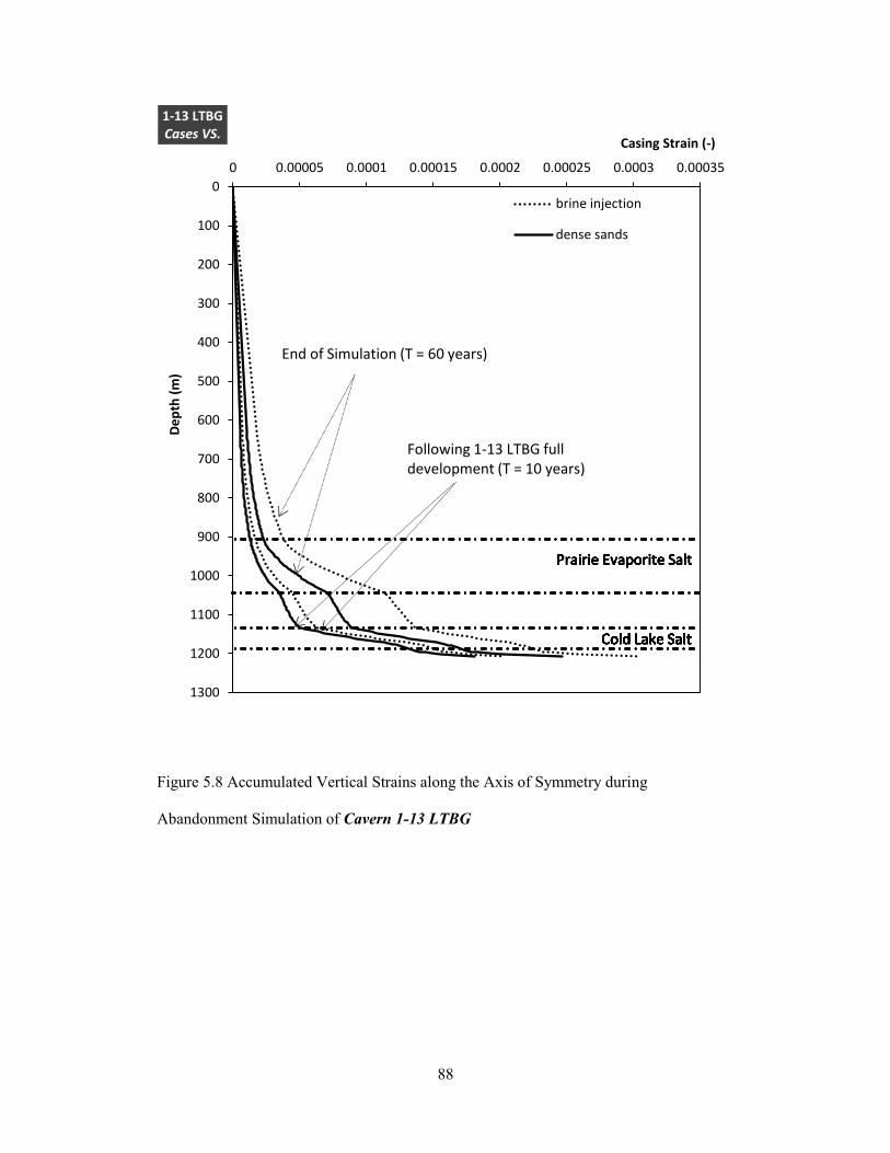
88
Figure 5.8 Accumulated Vertical Strains along the Axis of Symmetry during
Abandonment Simulation of Cavern 1-13 LTBG
0
100
200
300
400
500
600
700
800
900
1000
1100
1200
1300
0 0.00005 0.0001 0.00015 0.0002 0.00025 0.0003 0.00035D
ep
th (
m)
Casing Strain (-)
1-13 LTBG Cases VS.
brine injection
dense sands
Cold Lake Salt
Prairie Evaporite Salt
Following 1-13 LTBG full development (T = 10 years)
Cold Lake Salt
Prairie Evaporite Salt
Cold Lake Salt
Prairie Evaporite Salt
Cold Lake Salt
Prairie Evaporite Salt
Cold Lake Salt
Prairie Evaporite Salt
Cold Lake Salt
Prairie Evaporite Salt
Cold Lake Salt
Prairie Evaporite Salt
Cold Lake Salt
Prairie Evaporite Salt
Cold Lake Salt Cold Lake Salt Cold Lake Salt Cold Lake Salt Cold Lake Salt Cold Lake Salt Cold Lake Salt Cold Lake Salt Cold Lake Salt Cold Lake Salt Cold Lake Salt
End of Simulation (T = 60 years)

89
Figure 5.9 Surface Subsidence Plot under 1-13 LTBG brine case
-12
-10
-8
-6
-4
-2
0
-2000 -1500 -1000 -500 0 500 1000 1500 2000Su
rfac
e S
ub
sid
en
ce (
mm
)
Radial Distance (m) 1-13 LTBG brine case
1-yr aban (T=11years)
2-yr aban (T=12years)
5-yr aban (T=15years)
10-yr aban (T=20yeras)
20-yr aban (T=30years)
50-yr aban (T=60years)
1-13Well

90
Figure 5.10 Surface Subsidence Plot under 1-13 LTBG dense case
-12
-10
-8
-6
-4
-2
0
-2000 -1500 -1000 -500 0 500 1000 1500 2000Su
rfac
e S
ub
sid
en
ce (
mm
)
Radial Distance (m) 1-13 LTBG dense case
1-yr aban (T=11years)
2-yr aban (T=12years)
5-yr aban (T=15years)
10-yr aban (T=20yeras)
20-yr aban (T=30years)
50-yr aban (T=60years)
1-13Well

91
Figure 5.11 Predicted Maximum Surface Subsidence over Time (1-13 LTBG)
Table 5.2 Summarized Simulation Results for Cavern 1-13 LTBG
1-13 LTBG brine 1-13 LTBG dense
T = 10 years T = 60 years T = 10 years T = 60 years
Maximum Surface
Subsidence (mm) 3.99 10.52 3.18 6.47
Maximum Casing
Strains 0.000204 0.000305 0.000180 0.000246
Cavern Closure (%) 0 2.47 0 1.10
Minimum DSR 1.96 2.41 2.66 3.21
Minimum SSR 3.21 3.28 3.21 3.32
0.00
2.00
4.00
6.00
8.00
10.00
12.00
0 10 20 30 40 50 60
Max
imu
m S
urf
ace
Su
bsi
de
nce
(m
m)
Simulation Time (years)
1-13 LTBG Cases VS.
brine case
dense case
1-13LTBG Creation
1-13LTBG Abandoned
50-year Abandonment

92
5.3 Long-term Abandonment Behavior Simulation of Lotsberg
Caverns
The analysis initiated in Section 5.2 will be used for the complete scenario of the full
development of two horizontal Lotsberg caverns in FLAC3D
numerical modeling in this
section. Firstly, the contrast of instantaneous and sequential excavations will be
performed based on the specific injection conditions. Then using the sequential
excavation studies, the long-term abandonment creep behavior of the two Lotsberg
caverns will be simulated and analyzed for three different cavern internal pressure cases.
5.3.1 Long-term Abandonment Behavior Considering Instantaneous Excavation
Instantaneous excavations of both Cavern 1-13 LTBG and Cavern 8-13 LTBG were
performed simultaneously in the three-dimensional finite difference program. To simulate
the field operation, the existing 1-13 LTBG cavern will be filled with dense sand disposal
and sealed represented by a vertical pressure gradient of 0.072366 MPa/m, and the 8-13
Lotsberg cavern will be held at a constant brine pressure gradient of 0.011760 MPa/m.
The total creep simulation time for the two Lotsberg caverns is 50 years.
5.3.2 Long-term Abandonment Behavior Considering Sequential Excavations
The sequential excavations process and schedule of two Lotsberg caverns are described in
Table C.4, C.5 and C.6 (Appendix C). As shown, Cavern 1-13 LTBG will be solution
mined from 2006 to 2015, and then plugged and abandoned, followed by the 10-year
solution mining of Cavern 8-13 LTBG at the horizontal depth. The excavated depth of the
cavern filled with saturated brine in the previous year will be injected with waste disposal
and be held at a dense sands pressure in the following year. Similarly, one-year of creep
will be simulated after each excavation operation. Then the 1-13 LTBG cavern will be
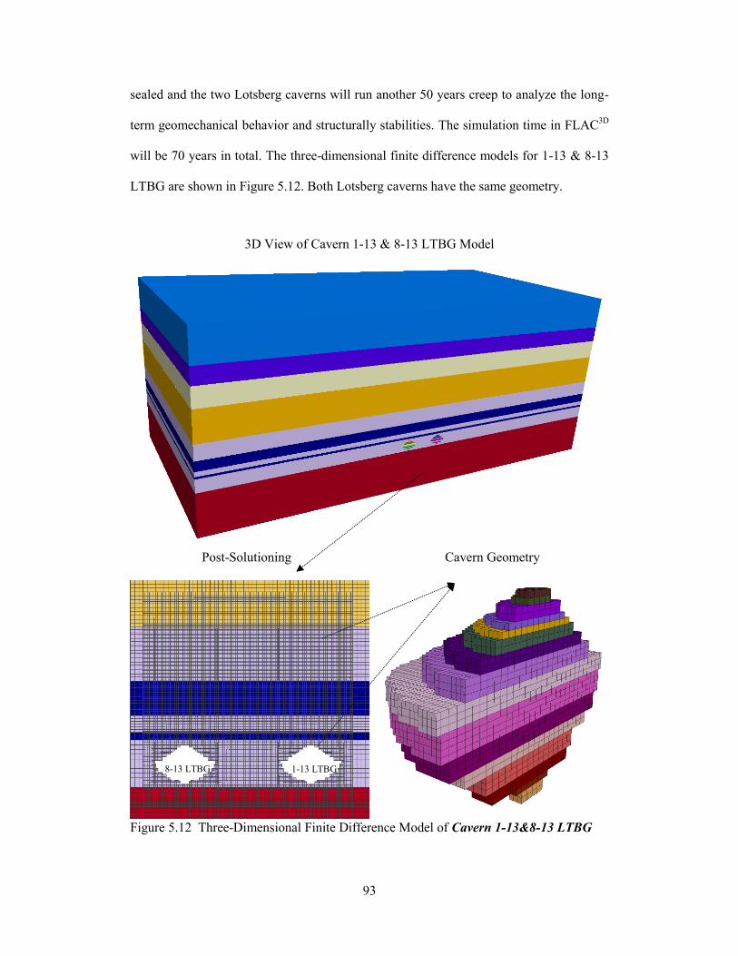
93
sealed and the two Lotsberg caverns will run another 50 years creep to analyze the long-
term geomechanical behavior and structurally stabilities. The simulation time in FLAC3D
will be 70 years in total. The three-dimensional finite difference models for 1-13 & 8-13
LTBG are shown in Figure 5.12. Both Lotsberg caverns have the same geometry.
3D View of Cavern 1-13 & 8-13 LTBG Model
Post-Solutioning
Cavern Geometry
Figure 5.12 Three-Dimensional Finite Difference Model of Cavern 1-13&8-13 LTBG
1-13 LTBG 8-13 LTBG

94
5.3.3 Results and Conclusions
Figure 5.13 illustrates the predicted DSR and SSR value plots over abandonment time and
Table 5.3 summaries the deformation simulation results for the instantaneous and
sequential excavations simulations. Similar conclusions can be made that, the
instantaneous excavation solution is able to predict approximately identical salt dilation
behavior surrounding the salt cavern and overlying nonsalt shear failure behavior as the
sequential excavation solutions at long-term abandonment. However, as for the short-
term structurally stability and integrity of the disposal salt caverns followed by the full
cavern development, instantaneous solutions may predict dilation failure of the salt units
around the caverns, which is not observed in sequential mining simulations. Moreover,
instantaneous excavations will underestimate the surface subsidence compared with
sequential simulations, with a reduced level of underestimation over creep time.
Additionally, instantaneous solutions will predict approximately double the cavern
volume loss for each disposal cavern of sequential excavations.
The simulation results of sequential solution under more cavern injection conditions are
given in Figure 5.14 to Figure 5.22. The deviatoric stresses development around the two
horizontal Lotsberg caverns due to caverns mining and operation was illustrated in Figure
5.14. In this Figure, Cavern 1-13 LTBG was filled with dense waste disposal and Cavern
8-13 LTBG was held at a brine pressure. The DSR and SSR values distributions are
provided in Figure 5.15 and Figure 5.16 respectively. As shown, the higher deviatoric
stresses of the salt units tend to flow around the lower-pressurized Cavern 8-13 LTBG
following the full development of the two Lotsberg caverns. Still no salt dilation
(DSR > 1) or non-salt shear failure (SSR > 1) was observed during the creation of both
Lotsberg caverns and after 50 years abandonment simulations, as the given DSR and SSR
values plots varied with simulation time in Figure 5.17. The DSR and SSR values

95
fluctuated during the cavern solution mining process due to the irregular excavations at
certain stages. Figure 5.17 also indicates that as long as either cavern is held at brine
pressure at abandonment, the minimum DSR value remains the same as the condition of
both caverns with brine inside. This is because the greatest potential for salt dilation is
usually located around the edge of the lower pressure-supported cavern. The potential of
salt dilation will be largely reduced once both caverns are plugged and abandoned with
dense waste disposal. However, the non-salt shear failure potential is not as sensitive as
the salt dilation with respect to the cavern internal pressures. The values of SSR do not
vary much with increased cavern pressure, and they stay constant at the end of simulation
for dense-brine and dense-dense case. The case of both caverns with brine show a slight
gradual decay on the SSR value but it may be expected the value will stay above one in
the foreseeable future. Additionally, the nonsalt shear failure behavior is noticeably
influenced by the excavations of horizontal adjacent caverns, independent of the injection
conditions.
The cavern closure behavior is presented in Figure 5.18 for Cavern 1-13&8-13 LTBG
under various cases. Conclusions can be drawn that its internal carrying pressure
dominates the cavern closure behavior, and it is not influenced much by the injection
conditions of the horizontal adjacent salt caverns. The volume loss of Cavern 8-13 LTBG
with brine is only reduced approximately 0.1% at 50-year creep if the adjacent Cavern
1-13 LTBG is held at an increased pressure from brine to dense sands. However, when
Cavern 8-13 LTBG is filled with disposal sands at abandonment, half of the cavern
volume loss will diminish and the shrinkage rate will reduce to 1.25% at the end of
simulations.
The accumulated casing strains for both Lotsberg caverns under dense-brine case are
shown in Figure 5.19. The casing strains of Cavern 1-13 LTBG increases from 0.00021

96
following the full development of both caverns to around 0.00029 at the end of
simulation. The corresponding casing strains for Cavern 8-13 LTBG is 0.00021 and
0.00033 respectively. Thus the casing strains of either cavern only increase slightly
during the 50-year abandonment time. This is because that the salt creep above the cavern
roof is relatively nonexistent following the whole period of cavern development and
operation, then the strains will remain nearly constant throughout the abandonment
simulation. The casing strains reacting with different cavern internal pressures of Cavern
1-13 LTBG and 8-13 LTBG were represented in Figure 5.20 and Figure 5.21 separately.
The figures suggested that the influence of the cavern injection conditions on the casing
strain is similar onto the cavern closure behavior. Cavern accumulated casing strains are
primarily determined by its internal cavity loads.
The surface subsidence plots for two horizontal Lotsberg caverns case were given in
Appendix C, Figures C.1 to C.3. The change of maximum surface subsidence for the two
caverns during simulation was illustrated in Figure 5.22. The maximum surface
subsidence when both caverns held brine pressure is around 25.54 mm, and this number
will reduce to nearly half when both caverns were abandoned with dense waste disposal.
The surface subsidence rate estimated from the plots for the brine-brine case is
approximately 0.2895 mm/year and for the dense-dense case is around 0.1261 mm/year.

97
Figure 5.13 Predicted DSR and SSR Value Evolution over Abandonment Time (1-
13&8-13 LTBG dense-brine)
Table 5.3 Comparison of Simulation Results for Instantaneous Excavations and
Sequential Excavations (1-13&8-13 LTBG dense-brine)
Instantaneous Excavations Sequential Excavations
1y
abandonment
50y
abandonment
1y
abandonment
50y
abandonment
Maximum Surface
Subsidence (mm) 4.3 16.4 8.6 19.2
Maximum Casing
Strains 0.000232 0.000315 0.000202 0.00032
Cavern 1-13 LTBG
Closure (%) 0.80 2.53 0.43 1.52
Cavern 8-13 LTBG
Closure (%) 1.42 4.76 0.13 2.66
0.00
0.50
1.00
1.50
2.00
2.50
3.00
3.50
4.00
4.50
5.00
0.00 10.00 20.00 30.00 40.00 50.00
Min
imu
m D
SR/S
SR V
alu
e
Abandonment Time (years)
1-13&8-13 LTBG dense-brine case
Instantaneous Excavation
Sequential Excavation
DSR
SSR
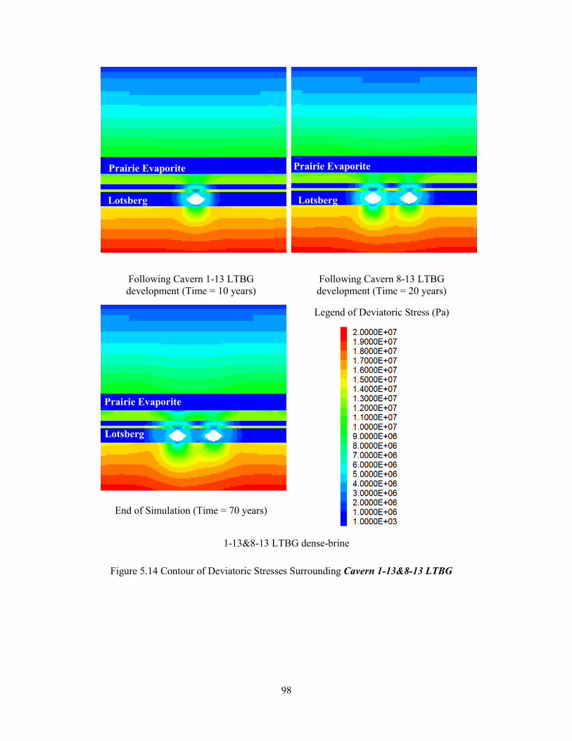
98
Following Cavern 1-13 LTBG
development (Time = 10 years)
Following Cavern 8-13 LTBG
development (Time = 20 years)
Legend of Deviatoric Stress (Pa)
End of Simulation (Time = 70 years)
1-13&8-13 LTBG dense-brine
Figure 5.14 Contour of Deviatoric Stresses Surrounding Cavern 1-13&8-13 LTBG
Lotsberg
Prairie Evaporite
Lotsberg
Prairie Evaporite
Lotsberg
Prairie Evaporite

99
Following Cavern 1-13 LTBG
development (Time = 10 years)
Following Cavern 8-13 LTBG
development (Time = 20 years)
Legend of DSR Value
End of Simulation (Time = 70 years)
1-13&8-13 LTBG dense-brine
Figure 5.15 DSR Value Distributions Surrounding Cavern 1-13&8-13 LTBG
Lotsberg
Prairie Evaporite
Lotsberg
Prairie Evaporite
Lotsberg
Prairie Evaporite
Minimum DSR = 2.66 Minimum DSR = 1.92
Minimum DSR = 2.34

100
Following Cavern 1-13 LTBG
development (Time = 10 years)
Following Cavern 8-13 LTBG
development (Time = 20 years)
Legend of SSR Value
End of Simulation (Time = 70 years)
1-13&8-13 LTBG dense-brine
Figure 5.16 SSR Value Distributions Surrounding Cavern 1-13&8-13 LTBG
Lotsberg
Prairie Evaporite
Lotsberg
Prairie Evaporite
Lotsberg
Prairie Evaporite
Minimum SSR = 3.21 Minimum SSR = 2.48
Minimum SSR = 2.49

101
Figure 5.17 DSR and SSR Value Varied with Simulation Time for Cavern 1-13&8-13
LTBG
0
0.5
1
1.5
2
2.5
3
3.5
4
4.5
5
0
1
2
3
4
5
6
7
8
0 10 20 30 40 50 60 70
Min
imu
m S
SR V
alu
e
Min
imu
m D
SR V
alu
e
Simulation Time (years)
1-13&8-13 LTBG Cases VS.
brine-brine case
dense-brine case
dense-dense case
1-13LTBG Creation
1-13LTBG Abandoned
8-13LTBG Creation
50-year Abandonment
8-13LTBG Abandoned
SSR
DSR

102
Figure 5.18 Predicted Caverns Closure as a Function of Time for Cavern 1-13&8-13
LTBG
0.0
0.5
1.0
1.5
2.0
2.5
3.0
3.5
0 10 20 30 40 50 60 70
Cav
ern
Clo
sure
(%
)
Simulation Time (years)
1-13&8-13LTBG Case VS.
brine-brine case
dense-brine case
dense-dense case
1-13LTBG Abandoned
8-13LTBG Abandoned
1-13LTBG Creation
8-13LTBG Creation
50-year Abandonment
Cavern 1-13LTBG
Cavern 8-13LTBG

103
Figure 5.19 Accumulated Vertical Strains along the Axis of Symmetry during
Abandonment Simulation (1-13&8-13 LTBG dense-brine)
0
100
200
300
400
500
600
700
800
900
1000
1100
1200
1300
0 0.00005 0.0001 0.00015 0.0002 0.00025 0.0003 0.00035D
ep
th (
m)
Casing Strain (-)
1-13&8-13 LTBG dense-brine case
Cavern 1-13LTBG (T=10years)
Cavern 1-13 LTBG (T=20 years)
Cavern 1-13 LTBG (T=70 years)
Cavern 8-13 LTBG (T=20 years)
Cavern 8-13 LTBG (T=70 years)
Cold Lake Salt
Prairie Evaporite Salt

104
Figure 5.20 Accumulated Casing Strains at the End of Simulation for Cavern 1-13
LTBG (1-13&8-13 LTBG)
0
100
200
300
400
500
600
700
800
900
1000
1100
1200
1300
0 0.00005 0.0001 0.00015 0.0002 0.00025 0.0003 0.00035 0.0004D
ep
th (
m)
Casing Strain of Cavern 1-13 LTBG (-) 1-13&8-13LTBG Cases VS.
brine-brine
dense-brine
dense-dense
Cold Lake Salt
Prairie Evaporite Salt

105
Figure 5.21 Accumulated Casing Strains at the End of Simulation for Cavern 8-13
LTBG (1-13&8-13 LTBG)
0
100
200
300
400
500
600
700
800
900
1000
1100
1200
1300
0 0.00005 0.0001 0.00015 0.0002 0.00025 0.0003 0.00035 0.0004D
ep
th (
m)
Casing Strain of Cavern 8-13 LTBG (-) 1-13&8-13LTBG Cases VS.
brine-brine
dense-brine
dense-dense
Cold Lake Salt
Prairie Evaporite Salt
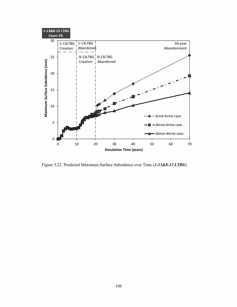
106
Figure 5.22 Predicted Maximum Surface Subsidence over Time (1-13&8-13 LTBG)
0
5
10
15
20
25
30
0 10 20 30 40 50 60 70
Max
imu
m S
urf
ace
Su
bsi
de
nce
(m
m)
Simulation Time (years)
1-13&8-13 LTBG Cases VS.
brine-brine case
dense-brine case
dense-dense case
1-13LTBG Creation
8-13LTBG Creation
1-13LTBG Abandoned
8-13LTBG Abandoned
50-year Abandonment

107
5.4 Long-term Abandonment Behavior Simulation of Vertical
Adjacent Caverns
5.4.1 Long-term Abandonment Behavior Considering Sequential Excavations
Two vertical adjacent caverns within one well are expected to have more issues with
structural stability and integrity of the salt and non-salt strata. The same sequential
excavation scenario will be applied onto the three-dimensional finite difference program
of two adjacent vertical 1-13 caverns located at Lotsberg and Prairie Evaporite formation
separately in this section. The solution-mining schedules of 1-13 LTBG & PRVP caverns
under three injection conditions are given in Figures C.7, C.9, and C.10 in Appendix C.
Cavern 1-13 LTBG was still excavated from the year 2006 and expected to be fully
developed and abandoned at the end of 2015. The solution mining creation of the uphole
Prairie Evaporite 1-13 cavern proceeds at the beginning of 2016 and it is assumed to be
plugged and sealed 10 years later in 2026 for permanent abandonment. Numerical
simulations of abandonment will last for 50 years and thus the total creep simulation time
will be 70 years in total. Figure 5.23 provides the three-dimensional finite difference
model of Cavern 1-13 LTBG & PRVP as well as the identical cavern geometry assigned
to both caverns.

108
3D View of Cavern 1-13 LTBG & PRVP Model
Post-Solutioning
Cavern Geometry
Figure 5.23 Three-Dimensional Finite Difference Model of Cavern 1-13 LTBG & PRVP
1-13 LTBG
1-13 PRVP

109
5.4.2 Results and Conclusions
The development of deviatoric stresses, distributions of DSR values and SSR values at the
site during the creation, operation, and abandonment of the two vertical 1-13 well caverns
under dense-brine case of most interest and are provided in Figure 5.24, Figure 5.25 and
Figure 5.26 respectively. Due to the fact that the cavern 1-13 LTBG fluid pressure relieve
the compressive stresses caused by the geological loads acting on the strata, the highest
potential for nonsalt shear failure will initialize within the Ernestina Lake Formation
some distance away from the cavern maximum edge. With the development of uphole
Prairie Evaporite cavern, the deviatoric stresses of the underlying strata decreased thus its
shear potential was reduced. Moreover, the excavation and fluid injection of the Cavern
1-13 PRVP results in the horizontal extension of the shear potential zone within the
Ernestina Lake units surrounding the downhole cavern where the deviatoric stresses
increases. However, the maximum deviatoric stresses decrease so that the minimum SSR
value grows from 3.21 to 3.57 during the development of the uphole cavern. Within the
same operational period, the salt dilation of lower cavern edge decayed with time due to
decreasing deviatoric stresses and the most dilation potential area moved to the outer
edge of the uphole cavern with DSR value equal to 1.79. The dilation potential of all salt
units slightly diminishes during the permanent abandonment of both caverns as it creeps.
In addition, the shear failure potential of non-salt overlying and underlying strata
decreases.
The change in values of DSR and SSR with simulation time for the two vertical caverns
under all considered cases is presented in Figure 5.27. It is expected that the potential of
salt dilation under dense-dense case is the least among three different cases. The figure
indicates that the minimum DSR value of the dense-brine case remains similar for the
value of both caverns filled with saturated brine. This is because the maximum salt

110
dilation potential always happens surrounding the salt cavern held at brine pressure.
Additionally, the SSR plots over simulation time show an interesting trend in the case of
asymmetrical injection situation (Cavern 1-13 LTBG with dense disposal and Cavern 1-
13 PRVP with brine) tend to have the least shear failure potential within the Ernestina
Lake than any of the other symmetrical injection cases. This is due to the unique
anisotropic initial in-situ stress distributions assigned onto the site, and the brine pressure
of the uphole cavern reduced the deviatoric stresses within the most potential shear layers.
All the predicted values in Figure 5.27 remain above 1 during simulations, indicating no
salt dilation or non-salt shear failure is expected for the two vertical adjacent caverns.
Additionally, the greatest shear failure potential always stays symmetrically of the
caverns within the Ernestina Lake Formation, and the solution mining of uphole cavern
has little influence on this potential shear zone.
The predicted cavern closures as a function of time was drawn in Figure 5.28. The given
curves verify that the cavern internal pressure itself only influences the cavern closure.
The closure ratio of uphole cavern held at brine pressure is predicted to reach
approximately 15.6% at the end of simulation, and this number will drop dramatically to
about 7.5% when the internal pressure is raised to dense sands support pressure. The
closure rate of the uphole cavern is significantly larger than the downhole cavern closure,
because the steady state creep rate for the Prairie Evaporite salt is higher than the
Lotsberg salt.
The simulated theoretical accumulated casing strains in FLAC3D
numerical modeling for
both caverns at dense-brine state are illustrated in Figure 5.29. It can be seen that the
casing strains of the uphole cavern bottom increased noticeably from 0.00185 to 0.00548
during the 50-year creep simulation. This is because the Cold Lake salt tends to flow into
the uphole cavern, where larger salt deviatoric stresses and cavern closure exist, and then

111
drag the upper part of the Cavern 1-13 LTBG casing significantly. Due to the upward
flow of the overlying rock, the strains of downhole casing shoes decreased mildly during
the permanent abandonment. As suggested that if J-55 grade steel casing is used for all
the disposal salt caverns, the casing will begin to yield at a strain of 0.0018 with ultimate
failure occurring at 0.0025 strain, the casing of Cavern 1-13 LTBG is predicted to yield
following the uphole cavern development and failure of the casing is expected to occur
within the 50-year abandonment. Figure 5.30 represents the case comparison in terms of
predicted casing strains for Cavern 1-13 LTBG&PRVP. The casing conditions turn out to
be reasonably for both waste-filled uphole and downhole caverns. As long as the disposal
cavern in Prairie Evaporite salt is held at brine pressure, casing failure is predicted to
occur for the downhole salt caverns.
The predicted maximum surface subsidence plots for cavern injection cases comparison
were shown in Figure 5.31. When the uphole cavern is brine-filled, the simulated
maximum surface vertical subsidence exceeds 0.08 m around the center of the cavern
field, which is only half the suggested subsidence value of 0.15 m by Van Sambeek
(2000). Also the surface subsidence will be significantly reduced to 0.046 m by injecting
the dense waste disposal into the uphole Prairie Evaporite cavern.

112
Following Cavern 1-13 LTBG
development (Time = 10 years)
Following Cavern 1-13 PRVP
development (Time = 20 years)
Legend of Deviatoric Stress (Pa)
End of Simulation (Time = 70 years)
1-13 LTBG & PRVP dense-brine
Figure 5.24 Contour of Deviatoric Stresses Surrounding Cavern 1-13 LTBG & PRVP
Lotsberg
Prairie Evaporite
Lotsberg
Prairie Evaporite
Lotsberg
Prairie Evaporite

113
Following Cavern 1-13 LTBG
development (Time = 10 years)
Following Cavern 1-13 PRVP
development (Time = 20 years)
Legend of DSR Value
End of Simulation (Time = 70 years)
1-13 LTBG & PRVP dense-brine
Figure 5.25 DSR Value Distributions Surrounding Cavern 1-13 LTBG & PRVP
Lotsberg
Prairie Evaporite
Lotsberg
Prairie Evaporite
Lotsberg
Prairie Evaporite
Minimum DSR = 2.66 Minimum DSR = 2.94
Minimum DSR = 1.79
Minimum DSR = 2.08
Minimum DSR = 3.51

114
Following Cavern 1-13 LTBG
development (Time = 10 years)
Following Cavern 1-13 PRVP
development (Time = 20 years)
Legend of SSR Value
End of Simulation (Time = 70 years)
1-13 LTBG & PRVP dense-brine
Figure 5.26 SSR Value Distributions Surrounding Cavern 1-13 LTBG & PRVP
Lotsberg
Prairie Evaporite
Lotsberg
Prairie Evaporite
Lotsberg
Prairie Evaporite
Minimum SSR = 3.21 Minimum SSR = 3.57
Minimum SSR = 3.8

115
Figure 5.27 DSR and SSR Value Varied with Simulation Time (Cavern 1-13 LTBG &
PRVP)
0
0.5
1
1.5
2
2.5
3
3.5
4
4.5
5
0
1
2
3
4
5
6
7
8
0 10 20 30 40 50 60 70
Min
imu
m S
SR V
alu
e
Min
imu
m D
SR V
alu
e
Simulation Time (years)
1-13 LTBG&PRVP Cases VS.
brine-brine case
dense-brine case
dense-dense case
1-13LTBG Creation
1-13LTBG Abandoned
1-13PRVP Creation
50-year Abandonment
1-13PRVP Abandoned
SSR
DSR

116
Figure 5.28 Predicted Caverns Closure as a Function of Time (1-13 LTBG & PRVP)
0.0
2.0
4.0
6.0
8.0
10.0
12.0
14.0
16.0
18.0
0 10 20 30 40 50 60 70
Cav
ern
Clo
sure
(%
)
Simulation Time (years)
1-13 LTBG&PRVP Cases VS.
brine-brine casedense-brine casedense-dense case
1-13LTBG Abandoned
1-13PRVP Abandoned
1-13LTBG Creation
1-13PRVP Creation
50-year abandonment
Cavern 1-13LTBG
Cavern 1-13PRVP

117
Figure 5.29 Accumulated Casing Strains during Simulation for Cavern 1-13 LTBG and
Cavern 1-13 PRVP (1-13 LTBG & PRVP dense-brine)
600
700
800
900
1000
1100
1200
1300
0 0.001 0.002 0.003 0.004 0.005 0.006D
ep
th (
m)
Casing Strain (-)
1-13 LTBG&PRVP dense-brine case
Following Cavern 8-13 LTBGDevelopment (T=20years)
End of 50-year abandonmentSimulation (T=70years)
Cold Lake Salt
Prairie Evaporite Salt
Lotsberg Salt
Cavern 1-13 PRVP
Cavern 1-13 LTBG

118
Figure 5.30 Accumulated Casing Strains during Simulation for Cavern 1-13 LTBG and
Cavern 1-13 PRVP (1-13 LTBG & PRVP)
600
700
800
900
1000
1100
1200
1300
0 0.001 0.002 0.003 0.004 0.005 0.006D
ep
th (
m)
Casing Strain (-)
1-13 LTBG&PRVP Cases VS.
brine-brine case
dense-brine case
dense-dense case
Cold Lake Salt
Prairie Evaporite Salt
Lotsberg Salt
Cavern 1-13 PRVP
Cavern 1-13 LTBG

119
Figure 5.31 Predicted Maximum Surface Subsidence over Time (1-13 LTBG & PRVP)
0
10
20
30
40
50
60
70
80
90
0 10 20 30 40 50 60 70
Max
imu
m S
urf
ace
Su
bsi
de
nce
(m
m)
Simulation Time (years)
1-13 LTBG&PRVP Cases VS.
brine-brine case
dense-brine case
dense-dense case
1-13LTBG Creation
1-13PRVP Creation
1-13LTBG Abandoned
1-13PRVP Abandoned
50-year Abandonment
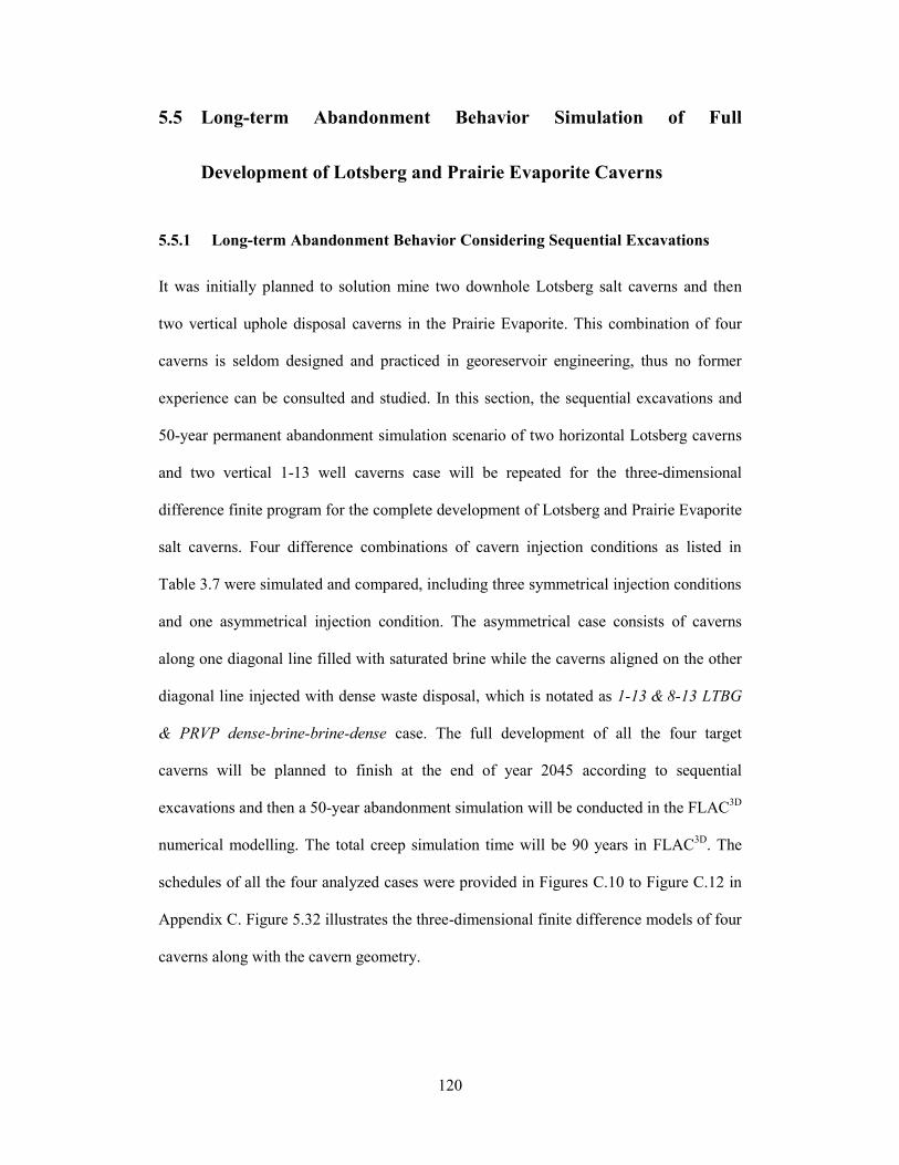
120
5.5 Long-term Abandonment Behavior Simulation of Full
Development of Lotsberg and Prairie Evaporite Caverns
5.5.1 Long-term Abandonment Behavior Considering Sequential Excavations
It was initially planned to solution mine two downhole Lotsberg salt caverns and then
two vertical uphole disposal caverns in the Prairie Evaporite. This combination of four
caverns is seldom designed and practiced in georeservoir engineering, thus no former
experience can be consulted and studied. In this section, the sequential excavations and
50-year permanent abandonment simulation scenario of two horizontal Lotsberg caverns
and two vertical 1-13 well caverns case will be repeated for the three-dimensional
difference finite program for the complete development of Lotsberg and Prairie Evaporite
salt caverns. Four difference combinations of cavern injection conditions as listed in
Table 3.7 were simulated and compared, including three symmetrical injection conditions
and one asymmetrical injection condition. The asymmetrical case consists of caverns
along one diagonal line filled with saturated brine while the caverns aligned on the other
diagonal line injected with dense waste disposal, which is notated as 1-13 & 8-13 LTBG
& PRVP dense-brine-brine-dense case. The full development of all the four target
caverns will be planned to finish at the end of year 2045 according to sequential
excavations and then a 50-year abandonment simulation will be conducted in the FLAC3D
numerical modelling. The total creep simulation time will be 90 years in FLAC3D
. The
schedules of all the four analyzed cases were provided in Figures C.10 to Figure C.12 in
Appendix C. Figure 5.32 illustrates the three-dimensional finite difference models of four
caverns along with the cavern geometry.
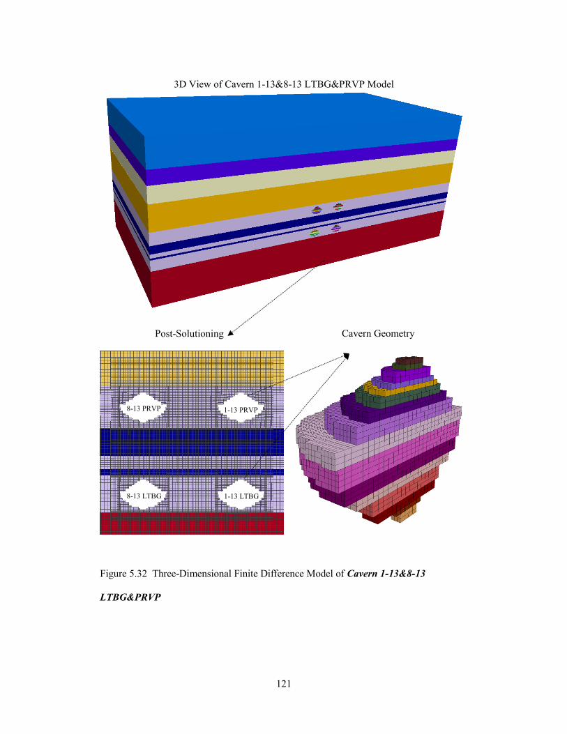
121
3D View of Cavern 1-13&8-13 LTBG&PRVP Model
Post-Solutioning
Cavern Geometry
Figure 5.32 Three-Dimensional Finite Difference Model of Cavern 1-13&8-13
LTBG&PRVP
1-13 LTBG
1-13 PRVP
8-13 LTBG
8-13 PRVP

122
5.5.2 Results and Conclusions
The caverns of asymmetrical injection conditions are of most research interest because of
their unpredictable long-term geomechanical behavior, as compared with other
symmetrical cases. Figure 5.33, Figure 5.34 and Figure 5.35 demonstrates the deviatoric
stresses, DSR values and SSR values contours evolution during the cavern development,
operation, and abandonment of the asymmetrical case respectively. As shown, the
deviatoric stresses generated on the upper-dense cavern side are higher than the upper-
brine cavern side at the end of simulation at this project site assigned specific in-situ
stresses. Thus, the most potential of non-salt shear failure is initially expected to occur on
the centre of the four caverns within the Ernestina Lake Formation prior to the
introduction of 8-13 PRVP cavern. Following the full development of all caverns the
most potential shear failure will align symmetrically along the lower brine-filled 8-13
LTBG cavern within the Ernestina Lake units, as well as the underlying formation which
needs to be paid attention due to the large area of low SSR value along the diagonal line.
However, this potential of failure diminishes with time due to the salt flow induced
decreasing deviatoric stress of the nonsalt strata. The greatest potential for salt dilation is
always predicted on the outer edge of the newly abandoned brine-filled caverns. The last
excavated 8-13 PRVP cavern shows very low potential of salt dilation, and the high
dilation zone within the Prairie Evaporite Formation diminishes during permanent
abandonment. On the contrary, the potential salt dilation of the Lotsberg salt on the left of
the lower brine-filled 8-13 LTBG Cavern shows a trend of expansion resulting from the
decreasing deviatoric stresses. Figure 5.36 depicts the minimum DSR and SSR values
observed of all geological units during simulations varied with time for cases comparison.
No salt dilation or non-salt shear failure is predicated during the simulation time. The
potential of nonsalt shear failure increases dramatically due to the solution mining of

123
brine-filled horizontal Lotsberg cavern along with the decreasing SSR value, and then
reduces slightly during the development of uphole Prairie Evaporite caverns. The separate
DSR value of each cavern during the 90-year creep simulation is shown in Figure 5.37,
and it indicates that the salt dilation potential along the cavern edge of each cavern during
the cavern creation is mainly determined by its internal pressures and will be influenced
at a certain level by the excavations of horizontal adjacent caverns. However, the ultimate
potential of salt dilation is largely and significantly dominated by the injection conditions
of the cavern itself, no matter the cavern internal pressure situations of the pre-existing
surrounding salt caverns.
Figure 5.38 gives the predicted cavern closure for each cavern as a function of simulation
time under all injection situations. The uphole Prairie Evaporite caverns shrinks
remarkably more than the lower Lotsberg caverns due to higher steady state creep rate.
The suggested conclusion that the cavern closure is totally determined by the cavern
internal pressure itself is verified again. The final closure of the uphole brine caverns at
the end of 90-year simulation exceeds 18% and it will drop approximately to half of the
value when the internal pressure increases to the dense sands support pressure. The
shrinkage rate of downhole Lotsberg caverns is within 2% even under brine-filled
conditions due to small steady state creep rate.
The predicted accumulated casing strains of each cavern under asymmetrical injection
conditions are depicted in Figure 5.39 and Figure 5.40. On the side of upper-dense and
lower-brine caverns, all the maximum casing strains are at the similar level and within the
casing yield limit of value of 0.0018. However, on the other side of upper-brine and
lower-dense side, the maximum of the Cavern 1-13 LTBG casing strains will exceed the
casing failure limit of 0.0025 value. This is due to the much higher creep rate and cavern
closure rate of the Prairie Evaporite units. If the PRVP cavern is injected with dense solid

124
waste, the cavern shrinkage will slow down due to high cavern support pressure and then
the casing dragging will be reduced as compared to the brine-filled case. Figure 5.41 and
Figure 5.42 illustrates the casing strains for cases comparison. Only the case of caverns
all filled with dense sands will ensure the casing strains remains within the yield limit and
no casing tensile failure is predicted during the simulations.
The maximum surface subsidence plots for case comparison were provided in Figure 5.43.
The cases of two uphole caverns filled with saturated brine will generate more than 0.15
m elevation change of the ground surface at site, resulting in effects on the area drainage
as suggested by Van Sambeek (2000). The surface subsidence rate estimated for the
asymmetrical case will be approximately 1.5224 mm/year, thus it is expected to exceed
0.15 m about 9 years later. Even the all dense-filled cavern case has a surface subsidence
growth rate of 0.9851 mm/year and will reach the threshold after another 55 years creep.

125
Following Cavern 8-13 LTBG
development (Time = 20 years)
Following Cavern 1-13 PRVP
development (Time = 30 years)
Following Cavern 8-13 PRVP
development (Time = 40 years) End of Simulation (Time = 90 years)
1-13&8-13 LTBG&PRVP
dense-brine-brine-dense
Legend of
Deviatoric
Stress
(Pa)
Figure 5.33 Contour of Deviatoric Stresses Surrounding Cavern 1-13&8-13
LTBG&PRVP
Lotsberg
Prairie Evaporite
Lotsberg
Prairie Evaporite
Lotsberg
Prairie Evaporite
Lotsberg
Prairie Evaporite

126
Following Cavern 8-13 LTBG
development (Time = 20 years)
Following Cavern 1-13 PRVP
development (Time = 30 years)
Following Cavern 8-13 PRVP
development (Time = 40 years) End of Simulation (Time = 90 years)
1-13&8-13 LTBG&PRVP
dense-brine-brine-dense
Legend of
DSR Value
(-)
Figure 5.34 DSR Value Distributions Surrounding Cavern 1-13&8-13 LTBG&PRVP
Lotsberg
Prairie Evaporite
Lotsberg
Prairie Evaporite
Lotsberg
Prairie
Evaporite
Minimum DSR = 1.92 Minimum DSR = 2.12
Minimum DSR = 1.78
Minimum DSR = 1.9
Minimum DSR = 2.4
Lotsberg
Prairie
Evaporite
Minimum DSR = 2.07
Minimum DSR = 2.67

127
Following Cavern 8-13 LTBG
development (Time = 20 years)
Following Cavern 1-13 PRVP
development (Time = 30 years)
Following Cavern 8-13 PRVP
development (Time = 40 years) End of Simulation (Time = 90 years)
1-13&8-13 LTBG&PRVP
dense-brine-brine-dense
Legend of
SSR Value
(-)
Figure 5.35 SSR Value Distributions Surrounding Cavern 1-13&8-13 LTBG&PRVP
Lotsberg
Prairie Evaporite
Minimum SSR = 2.49
Lotsberg
Prairie Evaporite
Minimum SSR = 2.63
Lotsberg
Prairie Evaporite
Minimum SSR = 2.97
Lotsberg
Prairie Evaporite
Minimum SSR = 3.18

128
Figure 5.36 Minimum DSR and SSR Value Varied with Simulation Time (Cavern 1-
13&8-13 LTBG&PRVP)
0.00
1.00
2.00
3.00
4.00
5.00
0.00
1.00
2.00
3.00
4.00
5.00
6.00
7.00
8.00
0 10 20 30 40 50 60 70 80 90
Min
imu
m S
SR V
alu
e
Min
imu
m D
SR V
alu
e
Simulation Time (years)
1-13&8-13 LTBG&PRVP Cases VS.
brine-brine-brine-brinedense-brine-brine-densedense-dense-brine-brinedense-dense-dense-dense
1-13 LTBG Creation
1-13 LTBG Abandoned
8-13 LTBG Creation
50-year Abandonment
8-13 LTBG Abandoned
SSR
DSR
1-13 PRVP Creation
1-13 PRVP Abandoned 8-13 PRVP Creation
8-13 PRVP Abandoned

129
Figure 5.37 DSR Value Evolution of Each Cavern during Simulation (1-13&8-13
LTBG&PRVP)
0.00
0.50
1.00
1.50
2.00
2.50
3.00
3.50
4.00
0 10 20 30 40 50 60 70 80 90
Min
imu
m D
SR V
alu
e
Simulation Time (years)
1-13&8-13 LTBG&PRVP Cases VS.
Cavern1-13 LTBGCavern 8-13 LTBGCavern 1-13 PRVPCavern 8-13 PRVP
50-year Abandonment
Green -> brine-brine-brine-brine Blue -> dense-brine-brine-dense Red -> dense-dense-brine-brine Black -> dense-dense-dense-dense

130
Figure 5.38 Predicted Caverns Closure as a Function of Time (1-13&8-13
LTBG&PRVP)
0.0
2.0
4.0
6.0
8.0
10.0
12.0
14.0
16.0
18.0
20.0
0 10 20 30 40 50 60 70 80 90
Cav
ern
Clo
sure
(%
)
Simulation Time (years)
1-13&8-13LTBG&PRVP Cases VS.
Cavern 1-13 LTBGCavern 8-13 LTBGCavern 1-13 PRVPCavern 8-13 PRVP
1-13 LTBG Abandoned
8-13 LTBG Abandoned
1-13 LTBG Creation
8-13 LTBG Creation
50-year abandonment
1-13 PRVP Creation
1-13 PRVP Anandoned
8-13 PRVP Creation
8-13 PRVP Anandoned
Green -> brine-brine-brine-brine Blue -> dense-brine-brine-dense Red -> dense-dense-brine-brine Black -> dense-dense-dense-dense

131
Figure 5.39 Accumulated Casing Strains during Simulation for Cavern 1-13 LTBG and
Cavern 1-13 PRVP (1-13 LTBG&PRVP dense-brine-brine-dense)
600
700
800
900
1000
1100
1200
1300
0 0.001 0.002 0.003 0.004 0.005 0.006D
ep
th (
m)
Casing Strain of 1-13 Well (-)
1-13&8-13 LTBG&PRVP dense-brine-brine-dense
Following Cavern 8-13 PRVPDevelopment (T=40years)
End of 50-year abandonmentSimulation (T=90years)
Cold Lake Salt
Prairie Evaporite Salt
Lotsberg Salt
Cavern 1-13 PRVP
Cavern 1-13 LTBG
132
Figure 5.40 Accumulated Casing Strains during Simulation for Cavern 8-13 LTBG and
Cavern 8-13 PRVP (1-13 LTBG&PRVP dense- brine-brine-dense)
600
700
800
900
1000
1100
1200
1300
0 0.0005 0.001 0.0015 0.002D
ep
th (
m)
Casing Strain of 8-13 Well (-)
1-13&8-13 LTBG&PRVP dense-brine-brine-dense
Following Cavern 8-13 PRVPDevelopment (T=40years)
End of 50-year abandonmentSimulation (T=90years)
Cold Lake Salt
Prairie Evaporite Salt
Lotsberg Salt
Cavern 8-13 PRVP
Cavern 8-13 LTBG

133
Figure 5.41 Accumulated Casing Strains during Simulation for 1-13 Well Caverns (1-
13&8-13 LTBG&PRVP)
600
700
800
900
1000
1100
1200
1300
0 0.001 0.002 0.003 0.004 0.005 0.006D
ep
th (
m)
Casing Strain of 1-13 Well (-)
1-13&8-13 LTBG&PRVP Cases VS.
brine-brine-brine-brinedense-brine-brine-desedense-dense-brine-brinedense-dense-dense-dense
Cold Lake Salt
Prairie Evaporite Salt
Lotsberg Salt
Cavern 1-13 PRVP
Cavern 1-13 LTBG
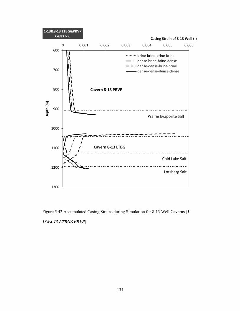
134
Figure 5.42 Accumulated Casing Strains during Simulation for 8-13 Well Caverns (1-
13&8-13 LTBG&PRVP)
600
700
800
900
1000
1100
1200
1300
0 0.001 0.002 0.003 0.004 0.005 0.006D
ep
th (
m)
Casing Strain of 8-13 Well (-)
1-13&8-13 LTBG&PRVP Cases VS.
brine-brine-brine-brine
dense-brine-brine-dense
dense-dense-brine-brine
dense-dense-dense-dense
Cold Lake Salt
Prairie Evaporite Salt
Lotsberg Salt
Cavern 8-13 PRVP
Cavern 8-13 LTBG

135
Figure 5.43 Predicted Maximum Surface Subsidence over Time (1-13&8-13
LTBG&PRVP)
0
20
40
60
80
100
120
140
160
180
0 10 20 30 40 50 60 70 80 90 100
Max
imu
m S
urf
ace
Su
bsi
de
nce
(m
m)
Simulation Time (years)
1-13&8-13 LTBG&PRVP Cases VS.
brine-brine-brine-brine case
dense-brine-brine-dense case
dense-dense-brine-brine case
dense-dense-dense-dense case
1-13LTBG Cavern Creation
8-13LTBG Cavern Creation
1-13LTBG Cavern Abandoned
8-13LTBG Cavern Abandoned
50-year Abandonment
1-13PRVP Cavern Creation
1-13PRVP Cavern Abandoned
8-13PRVP Cavern Creation
8-13PRVP Cavern Abandoned
136
5.6 Summary and Conclusions
A series of three-dimensional finite difference simulations were conducted in the FLAC3D
numerical modeling studies to evaluate the geomechanical performance of solution-
mined disposal salt caverns during development, operation and abandonment. The
geomechanical assessment includes the structurally stability and integrity analysis of the
disposal caverns throughout the simulation, the cavern volumetric closure behavior over
long-term abandonment, and the theoretical accumulated casing strains along the axis of
the symmetry of the caverns, as well as the induced surface subsidence at the site. The
numerical analysis were based on four cavern combinations, that is (1) single Lotsberg
cavern, (2) two horizontal adjacent Lotsberg caverns, (3) two vertical uphole and
downhole caverns, (4) two horizontal adjacent Lotsberg caverns and two uphole Prairie
Evaporite caverns. For each cavern combination, various cavern injection conditions were
considered and compared to study the influence of cavern internal pressure onto the long-
term geomechanical behavior of the disposal salt caverns. Additionally, two different
simulation methods for the cavern creation, including instantaneous excavations and
sequential excavations, were simulated and compared to analyze its influence in predicted
results.
Main conclusions derived from the various numerical simulations are listed as follows:
The instantaneous excavation solutions used to simulate the cavern solution-
mining development process can predict similar long-term abandonment salt
dilation behavior surrounding the target caverns as well as the nonsalt overlying
shear failure behavior as sequential excavation solutions. However, the
instantaneous simulations tend to predict dilation failure of the salt units
surrounding caverns following the full cavern development in terms of short-term

137
structural stability and integrity, which can be considered to be more conservative
than sequential solutions. Additionally, the instantaneous excavations will
overestimate the cavern volumetric shrinkage at almost double the sequential
excavations, but the predicted surface subsidence is less than the value of
sequential solutions.
As long as no salt dilation is observed during the development of salt caverns,
then the cavern stability and integrity will not be affected by the salt dilation
within permanent cavern abandonment, because the salt dilation potential will
slightly diminished during the permanent abandonment as the salt creeps. The
most salt dilation potential is always predicted at the outer edge of newly mined
and abandoned brine-filled caverns. In addition, the edge salt dilation behavior
for each cavern during cavern creations is mainly dependent on its internal
pressures, and will affected at a certain level by the excavations of horizontal
adjacent caverns. However, the ultimate salt dilation potential is totally
dominated by the injection conditions of the cavern itself, no matter the cavern
internal pressures of pre-existing adjacent caverns. The development of uphole
Prairie Evaporite caverns shows little influence on the salt dilation behavior of
lower Lotsberg disposal caverns. Moreover, for any cavern combination, the
potential of salt dilation will be significantly diminished with the disposal of
waste sands into the salt caverns as compared with the brine-filled caverns. One
thing needs to mention is that for the four cavern case under asymmetrical
injection conditions, the salt dilation potential area surrounding the lower brine-
filled cavern shows a trend of expansion, which is usually supposed to decay for
other studied cases.
The cavern internal pressures have little impact on the nonsalt shear failure
potential of the overlying strata based on the specific in-situ stresses conditions

138
assigned on the geological strata. However, the shear failure behavior of the
nonsalt overlying units is remarkably influenced by the solution-mining of
adjacent horizontal caverns, independent of its injection conditions. The greatest
shear failure potential for all cavern combinations is always located
symmetrically of the caverns within the overlying Ernestina Lake Formation, and
the solution mining of uphole cavern has little influence onto this potential shear
zone. If no shear failure occurs during the cavern creation, then no more shear
expected during the long-term abandonment. However, this conclusion is only
based on the specific lithostatic stresses distribution and may not applicable for
other geological conditions.
Cavern closure behavior is depended on the cavern internal pressures and the
steady state creep rate of the salt strata. For both brine and waste injection, the
cavern internal pressure is assumed to be constant during the long-term
simulation. However, the cavern shrinkage will pressurize the caverns and the
internal pressure will increase, which will in turn lead to the decrease of the
cavern closure rate. It can be concluded that its internal carrying pressure
dominates the cavern volumetric closure, and the horizontally adjacent salt
caverns and their injection conditions will not be affect it. For the salt cavern site
in this thesis, where the Prairie Evaporite Formation has a higher steady state
creep rate than the Lotsberg Formation, the volume loss of the uphole caverns
during abandonment is significantly larger than the downhole salt caverns. Thus
the development and operation of Prairie Evaporite caverns should be paid
greater attention to its potential storage volume loss and the corresponding
economic costs. However, if the uphole caverns can be filled with dense waste
disposal at abandonment, its cavern closure will be significantly reduced to less
139
than half of the brine-filled conditions and accepted volume shrinkage will be
expected during permanent abandonment.
The casing strains are predicted to be increased greatly within the salt formations
due to its creep flow vertically. The cavern internal support pressure itself
primarily determines the accumulated casing strains of each cavern. If caverns
only exist within the Lotsberg Formation, no yielding or tensile failure during
permanent abandonment is predicted. However, if uphole and downhole caverns
are excavated vertically aligned within the same well, the casings of the lower
Lotsberg caverns is predicted to yield or failed during 50-year abandonment as
long as the upper Prairie Evaporite caverns abandoned with saturated brine, if J-
55 grade steel casing used for this project. The condition of all caverns filled with
solid waste will relieve this casing stretching performance significantly and the
casing strains will be within the yield limit during 50-years abandonment
simulation.
The predicted surface is quite small for sole cavern case and two horizontal
Lotsberg caverns case. According to Van Sambeek’s suggestion, the elevation
change of less than about 0.15 m will not affect the area drainage significantly.
When vertical uphole caverns involved, the surface subsidence is largely
determined by the pressure conditions of Prairie Evaporite caverns. As long as
the uphole cavern is filled with brine, the surface subsidence will increase
dramatically even the downhole Lotsberg caverns are filled with dense waste. For
the four cavern case, the largely induced surface subsidence will be of the most
concern and potential damages onto the surface facilities and area drainage may
be brought onto the site, because that even all the caverns injected with dense
waste, the maximum surface subsidence will reach 0.09 m at the end of

140
simulation and will grow at a rate of approximately 0.9851 mm/year, expected to
exceed the 0.15 m threshold in another 55 years.

141
6 CONCLUSIONS AND RECOMMENDATIONS
6.1 General
The overall growth in world population, the resulting increase in industrial activity and
the recognition of environment and health impacts from indiscriminate disposal of waste
products has led to the need for an alternative to traditional methods of land filling and
costly high temperature combustion for the management of wastes.
The disposal of oil field wastes into the purposely-built salt caverns becomes feasible and
legal since the Argonne National Laboratory had performed a preliminary technical and
legal evaluation of the subjects in 1996 as the requirement by the U.S. Department of
Energy. In the past decades, there has been an increased worldwide in the number of salt
caverns that are specifically solution-mined as storage facilities for hydrocarbon and
oilfield waste, rather than for only brine production or other chemical feedstock. Solution
mined caverns in salt formations are becoming a preferred method due to their favourable
and appreciable geomechanical properties including low permeability and high ductility.
Because the history of the salt cavern used for solid waste disposal is very limited, as well
as the information of the post-closure behavior of the disposal caverns monitored in the
field, more predictions and simulations of the geomechanical performance and response
of the waste-filled salt caverns during operation and permanent abandonment are required
to get a better knowledge of the potential long term risks associated with disposal waste
caverns.
The objective of this thesis has been to analyze the numerical observations of the
structural stability and integrity of the salt caverns plugged and abandoned with waste
disposal during its development, operation, and permanent abandonment, as well as the

142
failure potential of the overlying nonsalt caprocks and the associated cavern casings.
Multiple-cavern configurations were also considered and simulated under various cavern
injection conditions and the interactions between adjacent caverns were evaluated in the
three-dimensional finite difference models. It has been shown that for all the cavern
configurations simulated, the structural stability and integrity intensity of the salt caverns
will be highly increase once all the salt caverns are injected with oil filed waste disposal,
and the induced deformation and cavern volume loss will be significantly mitigated as
well. It is suggested to convert the hydrocarbon gas or liquid storage caverns to waste
disposal caverns at the end of their lives to prevent potential cavern collapse or relieve the
accompanying risks or environmental hazards. The following section provides specific
conclusions regarding each component of the research in this thesis.
6.2 Conclusions
To provide a degree of verification of how well the modeling approach and scenario can
reasonably represent the geomechanical performances of the salt caverns, sensitivity
analyses focused on parametric properties of the three-dimensional finite difference
programs were conducted over a wide-range. The following conclusions were
summarized:
The Ran-Tunnel gridding approach shows more sensitivity to the dilation
behavior of the salt strata, presents more conservative potential of stability loss of
the waste disposal salt caverns, and predicts more deformation of the geological
units than the Rad-Cylindrical gridding with higher efficiency.
The boundary effects onto the deformation behavior of the salt caverns can be
eliminated significantly by increasing the outer radius of the three-dimensional
model to more than 2000 m. However, the boundary size shows little effect on

143
the salt dilation surrounding the caverns and shear behavior of the non-salt
overlying units.
The creep timestep settings embedded in FLAC3D
program will influence the
analytical outcomes significantly and need to be fairly determined for the sake of
reasonable results as well as efficiency.
The elastic parameters used to characterize the salt mechanical behavior have
limited influences on the model deformation as well as the structural stability and
integrity of the salt caverns predicted in FLAC3D
simulations.
The Power law parameters for describe the salt deformation mechanism can
influence the deformation behavior and structural stability behavior significantly,
thus they need to accurately determined in the laboratory testing studies to
adequately present the geomechanical response of the disposal salt caverns.
Various three-dimensional finite simulations have been performed in FLAC3D
numerical studies to evaluate the geomechanical performance of solution-mined
disposal salt caverns during its development, operation and abandonment. Different
cavern combinations have been considered including up to four-multiple-cavern cases.
For each salt cavern, two injection situations were analyzed and compared to study
the influence of cavern pressures onto the long-term geomechanical behavior of the
disposal salt caverns. The conclusions were listed below:
The instantaneous-excavation solution used to simulate the cavern solution-
mining process predicts similar long-term structural stability and integrity
behavior of the salt caverns as the sequential-excavation approach. As for
short-term performance, the instantaneous-solution predicts salt dilation
following the full cavern development, which is not the case for sequential-

144
approach. Additionally, sequential-solution can give more reasonable
deformation and volumetric closure behavior than instantaneous-approach.
As long as no salt dilation is observed during the development of salt caverns,
then the cavern stability and integrity will not be affected by the salt dilation
within permanent cavern abandonment. The most salt dilation potential is
always predicted onto the outer edge of newly mined and abandoned brine-
filled caverns. The ultimate salt dilation potential is totally dominated by the
injection conditions of the cavern itself, not be influenced much by pre-
existing adjacent caverns. The development of uphole Prairie Evaporite
caverns shows little influence on the salt dilation behavior of lower Lotsberg
disposal caverns. However, the case of lower cavern is filled and brine while
the upper cavern is waste filled is not suggested from an engineering point
because the potential of salt dilation surrounding the lower brine-filled
caverns is ascending with abandonment time. The potential of salt dilation
will be significantly diminished with the disposal of waste sands into the salt
caverns compared with the brine-filled caverns, no matter the number of
existing caverns at that time.
For the specific-site conditions, the shear failure behavior of the nonsalt
overlying caprock is remarkably influenced by the solution-mined horizontal
adjacent caverns, rather than its internal cavern support pressure. The
solution mining of an uphole cavern has much less influence on the greatest
shear potential zone.
The volumetric closure behavior of the caverns is highly independent on its
cavern internal pressure and the steady-state creep rate of the ambient salt
strata and it will not be affected by the horizontal and vertical adjacent salt
caverns and their injection conditions. In this thesis, the volume loss of the

145
uphole Prairie Evaporite caverns during abandonment is significantly larger
than the downhole Lotsberg caverns under same injection conditions.
However, if the uphole caverns can be filled with dense waste disposal at
abandonment, its cavern closure will be significantly reduced to less than half
of the brine-filled conditions and accepted volume shrinkage will be expected
during permanent abandonment.
The accumulated casing strains of each cavern are primarily determined by
the cavern internal support pressure itself. The appearance of the uphole
Prairie Evaporite caverns filled with brine will lead to the potential tensile
failure of casings of the lower Lotsberg caverns, even if they were waste-
filled. This situation can be mitigated by injecting dense sands waste into the
upper caverns and the lower casing will stay safe at least within 50-year
abandonment after the development of all the caverns. This estimation is a
conservative failure estimate because it assumes that casing failure will not
be influenced by probable slippage or casing string resistance and other
causes.
At this specific site for disposal salt caverns, surface subsidence for only
Lotsberg caverns is quite small and within the tolerance. However, if the
Prairie Evaporite salt caverns are developed, the induced surface subsidence
will exceed the suggested affecting threshold during permanent abandonment
and cause damage to the ground facilities and structures as well as the area
drainage, even if the all the existing caverns were injected with dense waste.
6.3 Recommendations for Future Research
The following recommendations may be useful for future studies of geomechanical
assessment for waste disposal salt caverns:

146
Utilize a more suitable constitutive model for the behavior of the rocksalt, e.g.
WIPP model which is specially designed for the waste disposal salt caverns. The
Norton power law used in this thesis does not take into account of the
temperature effects onto the rocksalt creep rate. Although in-situ temperatures are
not significantly elevated, it is expected that the creep rates will increase and
accompanying with the growing cavern deformation and volumetric closure.
The knowledge of the initial stress state at the salt cavern site and the material
properties is of fundamental importance both for understanding the formation
behavior and the numerical modeling studies of waste disposal salt caverns. It
can be suggested to conduct a three-dimensional geomechanical history match
analysis of the field geotechnical instrumentation results.
The interpretation of the cavern internal caverns pressure representing the waste
disposal is a key factor for long-term cavern geomechanical behavior. It is highly
recommended that laboratory testing studies need to be conducted onto the waste
disposal to assess their geomechanical properties both pre- and post- injection
operation.
147
REFERENCES
Boulianne M., 2004. A Numerical Investigation of the Creep (Viscoplastic) Behavior of
Circular Opening and Pillar in Rocksalt. The 57th Canadian Geotechnical
Conference, Session 5G, 25-32 p.
Buchholz S. A., and Nielnd J. D., 2012. Geomechanical Analysis of Solid Disposal
Caverns for Canadian Natural Resources Limited Kirby In Situ Oil Sands
Project Alberta Canada. Prepared for Canadian Natural Resources Limited,
Topical Report RSI-2314, RESPEC, Rapid City, South Dakota, December.
Davidson, B. C., 1997. Salt Solution Caverns for Petroleum Industry Wastes. Society of
Petroleum Engineers, Dallas, Texas, 51- 61 p.
Duyvestyn, G. M., and Davidson B. C., 1998. Salt Solution Caverns for Petroleum
Industry Toxic Granular Solid Waste Disposal. Society of Petroleum Engineers,
Trondheim, Norway, 8-10 July, 239 – 246 p.
Gardner, G.H.F.; Gardner L.W., Gregory A.R., 1974. Formation Velocity and Density -
The Diagnostic Basics for Stratigraphic Traps. Geophysics 39, 770–780 p.
Goodman, R. E., 1980. Introduction to Rock Mechanics, John Wiley and Sons, New
York, NY.
Greenberg, M.L., Castagna, J.P., 1992. Shear-wave velocity estimation in porous rocks:
Theoretical formulation, preliminary verification and applications. Geophysical
Prospecting 40, 195–209.
Grobe, M., 2000. Distribution and Thickness of Salt within the Devonian Elk Point
Group, Western Canada Sedimentary Basin. Alberta Energy and Utilities Board,
Alberta Geological Survey.
Hamilton W.N.,1971. Salt in East-Central Alberta. Research Council of Alberta.
Heerden W.L., 1987. Comparison of Static and Dynamic Elastic Moduli of Rock
Material. Pretoria, South Africa: Council for Scientific and Industrial Research,
National Mechanical Engineering Research Institute. CSIR Research Report
646, 95 pages.
Herrmann, W., Wawersik, W.R., Lauson, H.S., 1980a. Analysis of Steady State Creep of
Southeastern New Mexico Bedded Salt. Sandia National Laboratories,
SAND80-0558.
Herrmann, W., Wawersik, W.R., Lauson, H.S., 1980b. Creep Curves and Fitting
Parameters for Southeastern New Mexico Bedded Salt. Sandia National
Laboratories, SAND80-0558.

148
Itasca Consulting Group, Inc., 2011. FLAC3D
Fast Lagrangian Analysis of Continua in 3
Dimensions, 5th Ed. (FLAC
3D Version 5.0), Minneapolis, MN.
Martínez-Martínez J., Benavente D., García-del-Cura, M.A., 2012. Comparion of the
Static and Dynamic Modulus in Carbonate Rocks. Bull Eng Geol Environ 71,
263-268.
Pierre B., Benoit B., and Mehdi K. J., 2005. Deep Salt Caverns Abandonment. Post-Ming
2005,
Retigan J. L., 1995. Numerical Modeling of Week Island Subsidence and Laboratory
Testing of Weeks Island Salt. Solution Mining Research Institute Spring
Meeting, New Orleans, Louisiana, April 30 – May 3, 0-21 p.
Rankine, W.J.R., 1857. On the stability of Loose Earth. Philosophical Transactions of the
Royal Society of London 147, 9–27.
RG2, 2013. Geomechanical Study for Salt Caverns: Laboratory Testing Results LIND
8B-WD-13-57-5W4. Project report prepared by Reservoir Geomechanics
Research Group (RG2) for Company, 99 p.
Savich, A.I., 1984. Generalized Relations between Static and Dynamic Indices of Rock
Deformability. Hydrotechnical Construction 18(8), 394-400.
Tomasko D., Elcock D., Veil J., and Caudle D., 1999. Risk Analysis for Disposing
Nonhazardous Oil Field Wastes in Salt Caverns. Performed under Argonne
Nation Lab Contract No. W-31-109-ENG-38, Argonne National
Laboratory,Argonne, Illinois, January.
Van Sambeek, L. L., 2000. An Introduction to Subsidence Over Salt and Potash Mining
Facilities. Solution Mining Research Institute Fall Meeting, San Antonio, TX,
October 15-18, 0-10 p.
Veil, J. A., Smith, K. P., and Tomasko D., 1998. Disposal of NORM-Contaminated Oil
Field Wastes in Salt Caverns. Prepared for U.S. Department of Energy, Office
of Fossil Energy under Contract W-31-109-ENG-38, Argonne National
Laboratory, Argonne, Illinois, August.
Veil, J., Elcock D., Raivel M., Caudle D., Ayers R.C., Grunewald B., 1996. Preliminary
Technical and Legal Evaluation of Disposing of Nonhazardous Oil Field Waste
into Salt Caverns. Prepared for the U.S. Department of Energy, Office of Fossil
Energy under Contract W-31-109-ENG-38, Argonne National Laboratory,
Argonne, Illinois, June.

149
APPENDIX A Geological Review
Fig
ure
A. 1 S
chem
atic
Form
atio
ns
of
the
Elk
Poin
t G
roup (
Mei
jer
Dre
es, 1
98
6)

150
F
igu
re A
. 2 C
onto
ur
of
Dep
th t
o P
rair
ie E
vap
ori
te F
orm
atio
n

151
Fig
ure
A. 3
Is
opac
h C
onto
ur
of
Pra
irie
Evap
ori
te F
orm
atio
n

152
F
igure
A.
4 C
onto
ur
of
Dep
th t
o C
old
Lak
e F
orm
atio
n

153
Fig
ure
A. 5 Is
opac
h C
onto
ur
of
Cold
Lak
e F
orm
atio
n
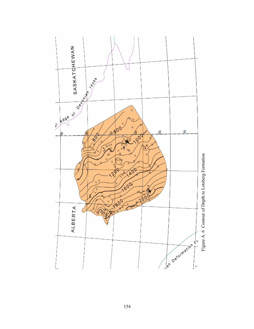
154
F
igure
A.
6 C
onto
ur
of
Dep
th t
o L
ots
ber
g F
orm
atio
n

155
Fig
ure
A. 7 Is
opac
h C
onto
ur
of
Lots
ber
g F
orm
atio
n

156
APPENDIX B Numerical Analytical Methodology
Table B. 1 Static and Dynamic Young’s Modulus Comparison for salt and Nonsalt
Units
Geological Unit
Dynamic
Young’s
Modulus
(GPa)
Static Young’s Modulus
(GPa)
Predicted Static Value
(Savich, 1984)
RokDoc UCS
Test
STC
Test
CMC
Test 227.1)(161.0 ds EE
Upper Caprock 30 - - - 10.45
Middle Caprock 6 - - - 1.45
Lower Caprock 10 - - - 2.72
Watt Mountain 40 22 3 - 14.88
Prairie Evaporite 37 2 N/A 7 13.52
Keg River 50 14 15 - 19.56
Cold Lake 37 - - - 13.52
Ernestina Lake 40 10 4 - 14.88
Lotsberg 37 3 - 7 13.52
Underburden 30 22 - 10.45
Notes: - indicates no available tests performed on the formation specimens in laboratory.

157
Figure B. 1 Cavern 1-13 LTBG 3D Configuration in WinUBro

158
Figure B. 2 Rad-Tunnel Gridding Method in FLAC3D
159
Figure B. 3 Rad-Cylindrical Gridding Method in FLAC3D

160
APPENDIX C Numerical Modeling Results
Table C. 1 Details of Cavern Sequential Excavations Steps
Excavation Lotsberg Cavern Prairie Evaporite Cavern
Step Depth from (m) Depth to (m) Depth from (m) Depth to (m)
1 1305 1301 1026 1022
2 1301 1296 1022 1017
3 1296 1290 1017 1011
4 1290 1283 1011 1004
5 1283 1275 1004 996
6 1275 1267 996 988
7 1267 1255 988 976
8 1255 1245 976 966
9 1245 1238 966 959
10 1238 1232 959 953
11 1232 1226 953 947
12 1226 1222 947 943
13 1222 1218 943 939
14 1218 1214 939 935
15 1214 1210 935 931

161
Table C. 2 Cavern 1-13 LTBG brine Case Solution Mining and Abandonment Schedule
Year Excavation
State Injection State
Simulation Time
(Year) Stage
2006 Step 1~3 Step 1~3 with brine 1 Operation
2007 Step 4~5 Step 4~5 with brine 2 Operation
2008 Step 6 Step 6 with brine 3 Operation
2009 Step 7 Step 7 with brine 4 Operation
2010 Step 8 Step 8 with brine 5 Operation
2011 Step 9 Step 9 with brine 6 Operation
2012 Step 10~11 Step 10~11 with brine 7 Operation
2013 Step 12~13 Step 12~13 with brine 8 Operation
2014 Step 14~16 Step 14~16 with brine 9 Operation
2015 10 Operation
2016 11 Abandonment
2017 12 Abandonment
2020 15 Abandonment
2025 20 Abandonment
2035 30 Abandonment
2065 60 Abandonment

162
Table C. 3 Cavern 1-13 LTBG dense Case Solution Mining and Abandonment Schedule
Year Excavation
State Injection State
Simulation
Time (Year) Stage
2006 Step 1~3 Step 1~3 with
brine 1 Operation
2007 Step 4~5 Step 4~5 with
brine
Step 1~3 with
sands 2 Operation
2008 Step 6 Step 6 with
brine
Step 4~5 with
sands 3 Operation
2009 Step 7 Step 7 with
brine
Step 6 with
sands 4 Operation
2010 Step 8 Step 8 with
brine
Step 7 with
sands 5 Operation
2011 Step 9 Step 9 with
brine
Step 8 with
sands 6 Operation
2012 Step 10~11 Step 10~11 with
brine
Step 9 with
sands 7 Operation
2013 Step 12~13 Step 12~13 with
brine
Step 10~11
with sands 8 Operation
2014 Step 14~16 Step 14~16 with
brine
Step 12~13
with sands 9 Operation
2015 Step 14~16
with sands 10 Operation
2016 11 Abandonment
2017 12 Abandonment
2020 15 Abandonment
2025 20 Abandonment
2035 30 Abandonment
2065 60 Abandonment
163
Table C. 4 Cavern 1-13&8-13 LTBG brine-brine Case Solution Mining and
Abandonment Schedule
Year Excavation
State Injection State
Simulation
Time (Year) Stage
1-13 LTBG Cavern
2006 Step 1~3 Step 1~3 with brine 1 Operation
2007 Step 4~5 Step 4~5 with brine 2 Operation
2008 Step 6 Step 6 with brine 3 Operation
2009 Step 7 Step 7 with brine 4 Operation
2010 Step 8 Step 8 with brine 5 Operation
2011 Step 9 Step 9 with brine 6 Operation
2012 Step 10~11 Step 10~11 with brine 7 Operation
2013 Step 12~13 Step 12~13 with brine 8 Operation
2014 Step 14~16 Step 14~16 with brine 9 Operation
2015 10 Operation
8-13 LTBG Cavern
2016 Step 1~3 Step 1~3 with brine 11 Operation
2017 Step 4~5 Step 4~5 with brine 12 Operation
2018 Step 6 Step 6 with brine 13 Operation
2019 Step 7 Step 7 with brine 14 Operation
2020 Step 8 Step 8 with brine 15 Operation
2021 Step 9 Step 9 with brine 16 Operation
2022 Step 10~11 Step 10~11 with brine 17 Operation
2023 Step 12~13 Step 12~13 with brine 18 Operation
2024 Step 14~16 Step 14~16 with brine 19 Operation
2025 20 Operation
2026 21 Abandonment
2027 22 Abandonment
2030 25 Abandonment
2035 30 Abandonment
2045 40 Abandonment
2075 70 Abandonment
164
Table C. 5 Cavern 1-13&8-13 LTBG dense-brine Case Solution Mining and
Abandonment Schedule
Year Excavation
State Injection State
Simulation
Time
(Year)
Stage
1-13 LTBG Cavern
2006 Step 1~3 Step 1~3 with
brine 1 Operation
2007 Step 4~5 Step 4~5 with
brine
Step 1~3 with
sands 2 Operation
2008 Step 6 Step 6 with
brine
Step 4~5 with
sands 3 Operation
2009 Step 7 Step 7 with
brine
Step 6 with
sands 4 Operation
2010 Step 8 Step 8 with
brine
Step 7 with
sands 5 Operation
2011 Step 9 Step 9 with
brine
Step 8 with
sands 6 Operation
2012 Step 10~11 Step 10~11 with
brine
Step 9 with
sands 7 Operation
2013 Step 12~13 Step 12~13 with
brine
Step 10~11 with
sands 8 Operation
2014 Step 14~16 Step 14~16 with
brine
Step 12~13 with
sands 9 Operation
2015 Step 14~16 with
sands 10 Operation
8-13 LTBG Cavern
2016 Step 1~3 Step 1~3 with
brine 11 Operation
2017 Step 4~5 Step 4~5 with
brine 12 Operation
2018 Step 6 Step 6 with
brine 13 Operation
2019 Step 7 Step 7 with
brine 14 Operation
2020 Step 8 Step 8 with
brine 15 Operation
2021 Step 9 Step 9 with
brine 16 Operation
2022 Step 10~11 Step 10~11 with
brine 17 Operation
2023 Step 12~13 Step 12~13 with
brine 18 Operation

165
2024 Step 14~16 Step 14~16 with
brine 19 Operation
2025 20 Operation
2026 21 Abandonment
2027 22 Abandonment
2030 25 Abandonment
2035 30 Abandonment
2045 40 Abandonment
2075 70 Abandonment
166
Table C. 6 Cavern 1-13&8-13 LTBG Dense-Dense-Case Solution Mining and
Abandonment Schedule
Year Excavation
State Injection State
Simulation
Time
(Year)
Stage
1-13 LTBG Cavern
2006 Step 1~3 Step 1~3 with
brine 1 Operation
2007 Step 4~5 Step 4~5 with
brine
Step 1~3 with
sands 2 Operation
2008 Step 6 Step 6 with
brine
Step 4~5 with
sands 3 Operation
2009 Step 7 Step 7 with
brine
Step 6 with
sands 4 Operation
2010 Step 8 Step 8 with
brine
Step 7 with
sands 5 Operation
2011 Step 9 Step 9 with
brine
Step 8 with
sands 6 Operation
2012 Step 10~11 Step 10~11 with
brine
Step 9 with
sands 7 Operation
2013 Step 12~13 Step 12~13 with
brine
Step 10~11 with
sands 8 Operation
2014 Step 14~16 Step 14~16 with
brine
Step 12~13 with
sands 9 Operation
2015 Step 14~16 with
sands 10 Operation
8-13 LTBG Cavern
2016 Step 1~3 Step 1~3 with
brine 11 Operation
2017 Step 4~5 Step 4~5 with
brine
Step 1~3 with
sands 12 Operation
2018 Step 6 Step 6 with
brine
Step 4~5 with
sands 13 Operation
2019 Step 7 Step 7 with
brine
Step 6 with
sands 14 Operation
2020 Step 8 Step 8 with
brine
Step 7 with
sands 15 Operation
2021 Step 9 Step 9 with
brine
Step 8 with
sands 16 Operation
2022 Step 10~11 Step 10~11 with
brine
Step 9 with
sands 17 Operation
2023 Step 12~13 Step 12~13 with
brine
Step 10~11 with
sands 18 Operation

167
2024 Step 14~16 Step 14~16 with
brine
Step 12~13 with
sands 19 Operation
2025 Step 14~16 with
sands 20 Operation
2026 21 Abandonment
2027 22 Abandonment
2030 25 Abandonment
2035 30 Abandonment
2045 40 Abandonment
2075 70 Abandonment

168
Table C. 7 Cavern 1-13 LTBG&PRVP brine-brine Case Solution Mining and
Abandonment Schedule
Year Excavation
State Injection State
Simulation
Time (Year) Stage
1-13 LTBG Cavern
2006 Step 1~3 Step 1~3 with brine 1 Operation
2007 Step 4~5 Step 4~5 with brine 2 Operation
2008 Step 6 Step 6 with brine 3 Operation
2009 Step 7 Step 7 with brine 4 Operation
2010 Step 8 Step 8 with brine 5 Operation
2011 Step 9 Step 9 with brine 6 Operation
2012 Step 10~11 Step 10~11 with brine 7 Operation
2013 Step 12~13 Step 12~13 with brine 8 Operation
2014 Step 14~16 Step 14~16 with brine 9 Operation
2015 10 Operation
1-13 PRVP Cavern
2016 Step 1~3 Step 1~3 with brine 11 Operation
2017 Step 4~5 Step 4~5 with brine 12 Operation
2018 Step 6 Step 6 with brine 13 Operation
2019 Step 7 Step 7 with brine 14 Operation
2020 Step 8 Step 8 with brine 15 Operation
2021 Step 9 Step 9 with brine 16 Operation
2022 Step 10~11 Step 10~11 with brine 17 Operation
2023 Step 12~13 Step 12~13 with brine 18 Operation
2024 Step 14~16 Step 14~16 with brine 19 Operation
2025 20 Operation
2026 21 Abandonment
2027 22 Abandonment
2030 25 Abandonment
2035 30 Abandonment
2045 40 Abandonment
2075 70 Abandonment

169
Table C. 8 Cavern 1-13 LTBG&PRVP dense-brine Case Solution Mining and
Abandonment Schedule
Year Excavation
State Injection State
Simulatio
n Time
(Year)
Stage
1-13 LTBG Cavern
2006 Step 1~3 Step 1~3 with
brine 1 Operation
2007 Step 4~5 Step 4~5 with
brine
Step 1~3 with
sands 2 Operation
2008 Step 6 Step 6 with
brine
Step 4~5 with
sands 3 Operation
2009 Step 7 Step 7 with
brine
Step 6 with
sands 4 Operation
2010 Step 8 Step 8 with
brine
Step 7 with
sands 5 Operation
2011 Step 9 Step 9 with
brine
Step 8 with
sands 6 Operation
2012 Step 10~11 Step 10~11 with
brine
Step 9 with
sands 7 Operation
2013 Step 12~13 Step 12~13 with
brine
Step 10~11 with
sands 8 Operation
2014 Step 14~16 Step 14~16 with
brine
Step 12~13 with
sands 9 Operation
2015 Step 14~16 with
sands 10 Operation
1-13 PRVP Cavern
2016 Step 1~3 Step 1~3 with
brine 11 Operation
2017 Step 4~5 Step 4~5 with
brine 12 Operation
2018 Step 6 Step 6 with
brine 13 Operation
2019 Step 7 Step 7 with
brine 14 Operation
2020 Step 8 Step 8 with
brine 15 Operation
2021 Step 9 Step 9 with
brine 16 Operation
2022 Step 10~11 Step 10~11 with
brine 17 Operation
2023 Step 12~13 Step 12~13 with
brine 18 Operation

170
2024 Step 14~16 Step 14~16 with
brine 19 Operation
2025 20 Operation
2026 21 Abandonment
2027 22 Abandonment
2030 25 Abandonment
2035 30 Abandonment
2045 40 Abandonment
2075 70 Abandonment

171
Table C. 9 Cavern 1-13 LTBG&PRVP dense-dense Case Solution Mining and
Abandonment Schedule
Year Excavation
State Injection State
Simulation
Time
(Year)
Stage
1-13 LTBG Cavern
2006 Step 1~3 Step 1~3 with
brine 1 Operation
2007 Step 4~5 Step 4~5 with
brine
Step 1~3 with
sands 2 Operation
2008 Step 6 Step 6 with
brine
Step 4~5 with
sands 3 Operation
2009 Step 7 Step 7 with
brine
Step 6 with
sands 4 Operation
2010 Step 8 Step 8 with
brine
Step 7 with
sands 5 Operation
2011 Step 9 Step 9 with
brine
Step 8 with
sands 6 Operation
2012 Step 10~11 Step 10~11 with
brine
Step 9 with
sands 7 Operation
2013 Step 12~13 Step 12~13 with
brine
Step 10~11
with sands 8 Operation
2014 Step 14~16 Step 14~16 with
brine
Step 12~13
with sands 9 Operation
2015 Step 14~16
with sands 10 Operation
1-13 PRVP Cavern
2016 Step 1~3 Step 1~3 with
brine 11 Operation
2017 Step 4~5 Step 4~5 with
brine
Step 1~3 with
sands 12 Operation
2018 Step 6 Step 6 with
brine
Step 4~5 with
sands 13 Operation
2019 Step 7 Step 7 with
brine
Step 6 with
sands 14 Operation
2020 Step 8 Step 8 with
brine
Step 7 with
sands 15 Operation
2021 Step 9 Step 9 with
brine
Step 8 with
sands 16 Operation
2022 Step 10~11 Step 10~11 with
brine
Step 9 with
sands 17 Operation
2023 Step 12~13 Step 12~13 with
brine
Step 10~11
with sands 18 Operation

172
2024 Step 14~16 Step 14~16 with
brine
Step 12~13
with sands 19 Operation
2025 Step 14~16
with sands 20 Operation
2026 21 Abandonment
2027 22 Abandonment
2030 25 Abandonment
2035 30 Abandonment
2045 40 Abandonment
2075 70 Abandonment

173
Table C. 10 Cavern 1-13&8-13 LTBG&PRVP Brine-Brine-Brine-Brine-Case
Solution Mining and Abandonment Schedule
Year Excavation
State Injection State
Simulation
Time (Year) Stage
1-13 LTBG Cavern
2006 Step 1~3 Step 1~3 with brine 1 Operation
2007 Step 4~5 Step 4~5 with brine 2 Operation
2008 Step 6 Step 6 with brine 3 Operation
2009 Step 7 Step 7 with brine 4 Operation
2010 Step 8 Step 8 with brine 5 Operation
2011 Step 9 Step 9 with brine 6 Operation
2012 Step 10~11 Step 10~11 with brine 7 Operation
2013 Step 12~13 Step 12~13 with brine 8 Operation
2014 Step 14~16 Step 14~16 with brine 9 Operation
2015 10 Operation
8-13 LTBG Cavern
2016 Step 1~3 Step 1~3 with brine 11 Operation
2017 Step 4~5 Step 4~5 with brine 12 Operation
2018 Step 6 Step 6 with brine 13 Operation
2019 Step 7 Step 7 with brine 14 Operation
2020 Step 8 Step 8 with brine 15 Operation
2021 Step 9 Step 9 with brine 16 Operation
2022 Step 10~11 Step 10~11 with brine 17 Operation
2023 Step 12~13 Step 12~13 with brine 18 Operation
2024 Step 14~16 Step 14~16 with brine 19 Operation
1-13 PRVP Cavern
2026 Step 1~3 Step 1~3 with brine 21 Operation
2027 Step 4~5 Step 4~5 with brine 22 Operation
2028 Step 6 Step 6 with brine 23 Operation
2029 Step 7 Step 7 with brine 24 Operation
2030 Step 8 Step 8 with brine 25 Operation
2031 Step 9 Step 9 with brine 26 Operation
2032 Step 10~11 Step 10~11 with brine 27 Operation
2033 Step 12~13 Step 12~13 with brine 28 Operation
2034 Step 14~16 Step 14~16 with brine 29 Operation
2035 30 Operation
8-13 PRVP
2036 Step 1~3 Step 1~3 with brine 31 Operation
2037 Step 4~5 Step 4~5 with brine 32 Operation
2038 Step 6 Step 6 with brine 33 Operation

174
2039 Step 7 Step 7 with brine 34 Operation
2040 Step 8 Step 8 with brine 35 Operation
2041 Step 9 Step 9 with brine 36 Operation
2042 Step 10~11 Step 10~11 with brine 37 Operation
2043 Step 12~13 Step 12~13 with brine 38 Operation
2044 Step 14~16 Step 14~16 with brine 39 Operation
2045 40 Operation
2046 41 Abandonment
2095 90 Abandonment

175
Table C. 11 Cavern 1-13&8-13 LTBG&PRVP Dense-Brine-Brine-Dense-Case Solution
Mining and Abandonment Schedule
Year Excavation
State Injection State
Simulation
Time (Year) Stage
1-13 LTBG Cavern
2006 Step 1~3 Step 1~3 with
brine 1 Operation
2007 Step 4~5 Step 4~5 with
brine
Step 1~3 with
sands 2 Operation
2008 Step 6 Step 6 with
brine
Step 4~5 with
sands 3 Operation
2009 Step 7 Step 7 with
brine
Step 6 with
sands 4 Operation
2010 Step 8 Step 8 with
brine
Step 7 with
sands 5 Operation
2011 Step 9 Step 9 with
brine
Step 8 with
sands 6 Operation
2012 Step 10~11 Step 10~11
with brine
Step 9 with
sands 7 Operation
2013 Step 12~13 Step 12~13
with brine
Step 10~11 with
sands 8 Operation
2014 Step 14~16 Step 14~16
with brine
Step 12~13 with
sands 9 Operation
2015 Step 14~16 with
sands 10 Operation
8-13 LTBG Cavern
2016 Step 1~3 Step 1~3 with
brine 11 Operation
2017 Step 4~5 Step 4~5 with
brine 12 Operation
2018 Step 6 Step 6 with
brine 13 Operation
2019 Step 7 Step 7 with
brine 14 Operation
2020 Step 8 Step 8 with
brine 15 Operation
2021 Step 9 Step 9 with
brine 16 Operation
2022 Step
10~11
Step 10~11
with brine 17 Operation
2023 Step
12~13
Step 12~13
with brine 18 Operation
2024 Step
14~16
Step 14~16
with brine 19 Operation
176
2025
1-13 PRVP Cavern
2026 Step 1~3 Step 1~3 with
brine 21 Operation
2027 Step 4~5 Step 4~5 with
brine 22 Operation
2028 Step 6 Step 6 with
brine 23 Operation
2029 Step 7 Step 7 with
brine 24 Operation
2030 Step 8 Step 8 with
brine 25 Operation
2031 Step 9 Step 9 with
brine 26 Operation
2032 Step
10~11
Step 10~11
with brine 27 Operation
2033 Step
12~13
Step 12~13
with brine 28 Operation
2034 Step
14~16
Step 14~16
with brine 29 Operation
2035 30 Operation
8-13 PRVP
2036 Step 1~3 Step 1~3 with
brine 31 Operation
2037 Step 4~5 Step 4~5 with
brine
Step 1~3 with
sands 32 Operation
2038 Step 6 Step 6 with
brine
Step 4~5 with
sands 33 Operation
2039 Step 7 Step 7 with
brine
Step 6 with
sands 34 Operation
2040 Step 8 Step 8 with
brine
Step 7 with
sands 35 Operation
2041 Step 9 Step 9 with
brine
Step 8 with
sands 36 Operation
2042 Step
10~11
Step 10~11
with brine
Step 9 with
sands 37 Operation
2043 Step
12~13
Step 12~13
with brine
Step 10~11 with
sands 38 Operation
2044 Step
14~16
Step 14~16
with brine
Step 12~13 with
sands 39 Operation
2045 Step 14~16 with
sands 40 Operation
2046 41 Abandonment
2095 90 Abandonment
177
Table C. 12 Cavern 1-13&8-13 LTBG&PRVP Dense-Dense-Brine-Brine-Case Solution
Mining and Abandonment Schedule
Year Excavation
State Injection State
Simulation
Time (Year) Stage
1-13 LTBG Cavern
2006 Step 1~3 Step 1~3 with
brine 1 Operation
2007 Step 4~5 Step 4~5 with
brine
Step 1~3 with
sands 2 Operation
2008 Step 6 Step 6 with
brine
Step 4~5 with
sands 3 Operation
2009 Step 7 Step 7 with
brine
Step 6 with
sands 4 Operation
2010 Step 8 Step 8 with
brine
Step 7 with
sands 5 Operation
2011 Step 9 Step 9 with
brine
Step 8 with
sands 6 Operation
2012 Step 10~11 Step 10~11
with brine
Step 9 with
sands 7 Operation
2013 Step 12~13 Step 12~13
with brine
Step 10~11 with
sands 8 Operation
2014 Step 14~16 Step 14~16
with brine
Step 12~13 with
sands 9 Operation
2015 Step 14~16 with
sands 10 Operation
8-13 LTBG Cavern
2016 Step 1~3 Step 1~3 with
brine 11 Operation
2017 Step 4~5 Step 4~5 with
brine
Step 1~3 with
sands 12 Operation
2018 Step 6 Step 6 with
brine
Step 4~5 with
sands 13 Operation
2019 Step 7 Step 7 with
brine
Step 6 with
sands 14 Operation
2020 Step 8 Step 8 with
brine
Step 7 with
sands 15 Operation
2021 Step 9 Step 9 with
brine
Step 8 with
sands 16 Operation
2022 Step
10~11
Step 10~11
with brine
Step 9 with
sands 17 Operation
2023 Step
12~13
Step 12~13
with brine
Step 10~11 with
sands 18 Operation
2024 Step
14~16
Step 14~16
with brine
Step 12~13 with
sands 19 Operation
2025 Step 14~16 with
sands

178
1-13 PRVP Cavern
2026 Step 1~3 Step 1~3 with
brine 21 Operation
2027 Step 4~5 Step 4~5 with
brine 22 Operation
2028 Step 6 Step 6 with
brine 23 Operation
2029 Step 7 Step 7 with
brine 24 Operation
2030 Step 8 Step 8 with
brine 25 Operation
2031 Step 9 Step 9 with
brine 26 Operation
2032 Step
10~11
Step 10~11
with brine 27 Operation
2033 Step
12~13
Step 12~13
with brine 28 Operation
2034 Step
14~16
Step 14~16
with brine 29 Operation
2035 30 Operation
8-13 PRVP
2036 Step 1~3 Step 1~3 with
brine 31 Operation
2037 Step 4~5 Step 4~5 with
brine 32 Operation
2038 Step 6 Step 6 with
brine 33 Operation
2039 Step 7 Step 7 with
brine 34 Operation
2040 Step 8 Step 8 with
brine 35 Operation
2041 Step 9 Step 9 with
brine 36 Operation
2042 Step
10~11
Step 10~11
with brine 37 Operation
2043 Step
12~13
Step 12~13
with brine 38 Operation
2044 Step
14~16
Step 14~16
with brine 39 Operation
2045 40 Operation
2046 41 Abandonment
2095 90 Abandonment

179
Table C. 13 Cavern 1-13&8-13 LTBG&PRVP Dense-Dense-Dense-Dense-Case
Solution Mining and Abandonment Schedule
Year Excavation
State Injection State
Simulation
Time (Year) Stage
1-13 LTBG Cavern
2006 Step 1~3 Step 1~3 with
brine 1 Operation
2007 Step 4~5 Step 4~5 with
brine
Step 1~3 with
sands 2 Operation
2008 Step 6 Step 6 with
brine
Step 4~5 with
sands 3 Operation
2009 Step 7 Step 7 with
brine
Step 6 with
sands 4 Operation
2010 Step 8 Step 8 with
brine
Step 7 with
sands 5 Operation
2011 Step 9 Step 9 with
brine
Step 8 with
sands 6 Operation
2012 Step 10~11 Step 10~11
with brine
Step 9 with
sands 7 Operation
2013 Step 12~13 Step 12~13
with brine
Step 10~11 with
sands 8 Operation
2014 Step 14~16 Step 14~16
with brine
Step 12~13 with
sands 9 Operation
2015 Step 14~16 with
sands 10 Operation
8-13 LTBG Cavern
2016 Step 1~3 Step 1~3 with
brine 11 Operation
2017 Step 4~5 Step 4~5 with
brine
Step 1~3 with
sands 12 Operation
2018 Step 6 Step 6 with
brine
Step 4~5 with
sands 13 Operation
2019 Step 7 Step 7 with
brine
Step 6 with
sands 14 Operation
2020 Step 8 Step 8 with
brine
Step 7 with
sands 15 Operation
2021 Step 9 Step 9 with
brine
Step 8 with
sands 16 Operation
2022 Step
10~11
Step 10~11
with brine
Step 9 with
sands 17 Operation
2023 Step
12~13
Step 12~13
with brine
Step 10~11 with
sands 18 Operation
2024 Step
14~16
Step 14~16
with brine
Step 12~13 with
sands 19 Operation
2025 Step 14~16 with
sands

180
1-13 PRVP Cavern
2026 Step 1~3 Step 1~3 with
brine 21 Operation
2027 Step 4~5 Step 4~5 with
brine
Step 1~3 with
sands 22 Operation
2028 Step 6 Step 6 with
brine
Step 4~5 with
sands 23 Operation
2029 Step 7 Step 7 with
brine
Step 6 with
sands 24 Operation
2030 Step 8 Step 8 with
brine
Step 7 with
sands 25 Operation
2031 Step 9 Step 9 with
brine
Step 8 with
sands 26 Operation
2032 Step
10~11
Step 10~11
with brine
Step 9 with
sands 27 Operation
2033 Step
12~13
Step 12~13
with brine
Step 10~11 with
sands 28 Operation
2034 Step
14~16
Step 14~16
with brine
Step 12~13 with
sands 29 Operation
2035 Step 14~16 with
sands 30 Operation
8-13 PRVP
2036 Step 1~3 Step 1~3 with
brine 31 Operation
2037 Step 4~5 Step 4~5 with
brine
Step 1~3 with
sands 32 Operation
2038 Step 6 Step 6 with
brine
Step 4~5 with
sands 33 Operation
2039 Step 7 Step 7 with
brine
Step 6 with
sands 34 Operation
2040 Step 8 Step 8 with
brine
Step 7 with
sands 35 Operation
2041 Step 9 Step 9 with
brine
Step 8 with
sands 36 Operation
2042 Step
10~11
Step 10~11
with brine
Step 9 with
sands 37 Operation
2043 Step
12~13
Step 12~13
with brine
Step 10~11 with
sands 38 Operation
2044 Step
14~16
Step 14~16
with brine
Step 12~13 with
sands 39 Operation
2045 Step 14~16 with
sands 40 Operation
2046 41 Abandonment
2095 90 Abandonment

181
Figure C. 1 Accumulated Vertical Strains along the Axis of Symmetry of Cavern 1-13
LTBG during Abandonment Simulation (1-13&8-13 LTBG brine-brine)
0
100
200
300
400
500
600
700
800
900
1000
1100
1200
1300
0 0.00005 0.0001 0.00015 0.0002 0.00025 0.0003 0.00035 0.0004D
ep
th (
m)
Casing Strain of Cavern 1-13LTBG (-)
1-13&8-13LTBG brine-brine case
Following Cavern 1-13 LTBGDevelopment (T=10years)
Following Cavern 8-13 LTBGDevelopment (T=20years)
End of 50-year abandonmentSimulation (T=70years)
Cold Lake Salt
Prairie Evaporite Salt

182
Figure C. 2 Accumulated Vertical Strains along the Axis of Symmetry of Cavern 8-13
LTBG during Abandonment Simulation (1-13&8-13 LTBG brine-brine)
0
100
200
300
400
500
600
700
800
900
1000
1100
1200
1300
0 0.00005 0.0001 0.00015 0.0002 0.00025 0.0003 0.00035 0.0004D
ep
th (
m)
Casing Strain of Cavern 8-13LTBG (-)
1-13&8-13 LTBG brine-brine case
Following Cavern 8-13 LTBGDevelopment (T=20years)
End of 50-year abandonmentSimulation (T=70years)
Cold Lake Salt
Prairie Evaporite Salt

183
Figure C. 3 Accumulated Vertical Strains along the Axis of Symmetry of Cavern 1-13
LTBG during Abandonment Simulation (1-13&8-13 LTBG dense-dense)
0
100
200
300
400
500
600
700
800
900
1000
1100
1200
1300
0 0.00005 0.0001 0.00015 0.0002 0.00025 0.0003D
ep
th (
m)
Casing Strain of Cavern 1-13LTBG (-)
1-13&8-13 LTBG dense-dense case
Following Cavern 1-13 LTBGDevelopment (T=10years)
Following Cavern 8-13 LTBGDevelopment (T=20years)
End of 50-year abandonmentSimulation (T=70years)
Cold Lake Salt
Prairie Evaporite Salt

184
Figure C. 4 Accumulated Vertical Strains along the Axis of Symmetry of Cavern 8-13
LTBG during Abandonment Simulation (1-13&8-13 LTBG dense-dense)
0
100
200
300
400
500
600
700
800
900
1000
1100
1200
1300
0 0.00005 0.0001 0.00015 0.0002 0.00025 0.0003D
ep
th (
m)
Casing Strain of Cavern 8-13LTBG (-)
1-13&8-13 LTBG dense-dense case
Following Cavern 8-13 LTBGDevelopment (T=20years)
End of 50-year abandonmentSimulation (T=70years)
Cold Lake Salt
Prairie Evaporite Salt

185
Figure C. 5 Surface Subsidence Plot (1-13&8-13 LTBG brine-brine)
-30
-25
-20
-15
-10
-5
0
-2000 -1500 -1000 -500 0 500 1000 1500 2000
Surf
ace
Su
bsi
de
nce
(m
m)
Radial Distance (m)
1-13&8-13 LTBG brine-brine case
1-year abandonment(T=21years)2-year abandonment(T=22year)5-year abandonment(T=25years)10-year abandonment(T=30yeras)20-year abandonment(T=40years)50-year abandonment(T=70years)
8-13Well 1-13Well
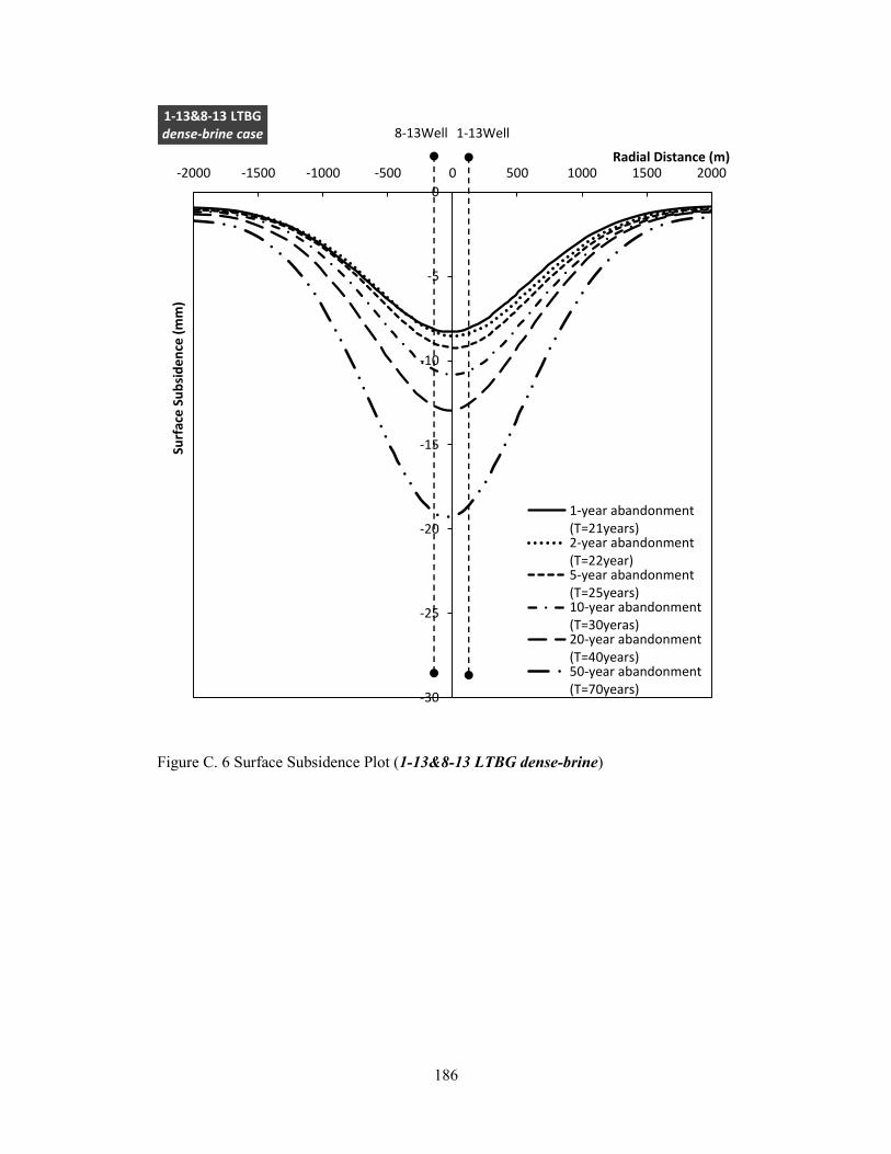
186
Figure C. 6 Surface Subsidence Plot (1-13&8-13 LTBG dense-brine)
-30
-25
-20
-15
-10
-5
0
-2000 -1500 -1000 -500 0 500 1000 1500 2000Su
rfac
e S
ub
sid
en
ce (
mm
)
Radial Distance (m)
1-13&8-13 LTBG dense-brine case
1-year abandonment(T=21years)2-year abandonment(T=22year)5-year abandonment(T=25years)10-year abandonment(T=30yeras)20-year abandonment(T=40years)50-year abandonment(T=70years)
8-13Well 1-13Well

187
Figure C. 7 Surface Subsidence Plot (1-13&8-13 LTBG dense-dense)
-30
-25
-20
-15
-10
-5
0
-2000 -1500 -1000 -500 0 500 1000 1500 2000Su
rfac
e S
ub
sid
en
ce (
mm
)
Radial Distance (m)
1-13&8-13 LTBG dense-dense case
1-year abandonment(T=21years)2-year abandonment(T=22year)5-year abandonment(T=25years)10-year abandonment(T=30yeras)20-year abandonment(T=40years)50-year abandonment(T=70years)
8-13Well 1-13Well

188
Figure C. 8 Accumulated Casing Strains during Simulation for Cavern 1-13 LTBG and
Cavern 1-13 PRVP (1-13 LTBG&PRVP brine-brine)
600
700
800
900
1000
1100
1200
1300
0 0.001 0.002 0.003 0.004 0.005 0.006D
ep
th (
m)
Casing Strain (-)
1-13 LTBG&PRVP brine-brine case
Following Cavern 8-13 LTBGDevelopment (T=20years)
End of 50-year abandonmentSimulation (T=70years)
Cold Lake Salt
Prairie Evaporite Salt
Lotsberg Salt
Cavern 1-13 PRVP
Cavern 1-13 LTBG

189
Figure C. 9 Accumulated Casing Strains during Simulation for Cavern 1-13 LTBG and
Cavern 1-13 PRVP (1-13 LTBG&PRVP dense-dense)
600
700
800
900
1000
1100
1200
1300
0 0.001 0.002 0.003 0.004 0.005 0.006D
ep
th (
m)
Casing Strain (-)
1-13 LTBG&PRVP dense-dense case
Following Cavern 8-13 LTBGDevelopment (T=20years)
End of 50-year abandonmentSimulation (T=70years)
Cold Lake Salt
Prairie Evaporite Salt
Lotsberg Salt
Cavern 1-13 PRVP
Cavern 1-13 LTBG

190
Figure C. 10 Surface Subsidence Plot (1-13LTBG&PRVP brine-brine)
-90
-80
-70
-60
-50
-40
-30
-20
-10
0
-2000 -1500 -1000 -500 0 500 1000 1500 2000Su
rfac
e S
ub
sid
en
ce (
mm
)
Radial Distance (m)
1-13 PRVP<BG brine-brine case
1-year abandonment(T=21years)2-year abandonment(T=22year)5-year abandonment(T=25years)10-year abandonment(T=30yeras)20-year abandonment(T=40years)50-year abandonment(T=70years)
1-13Well
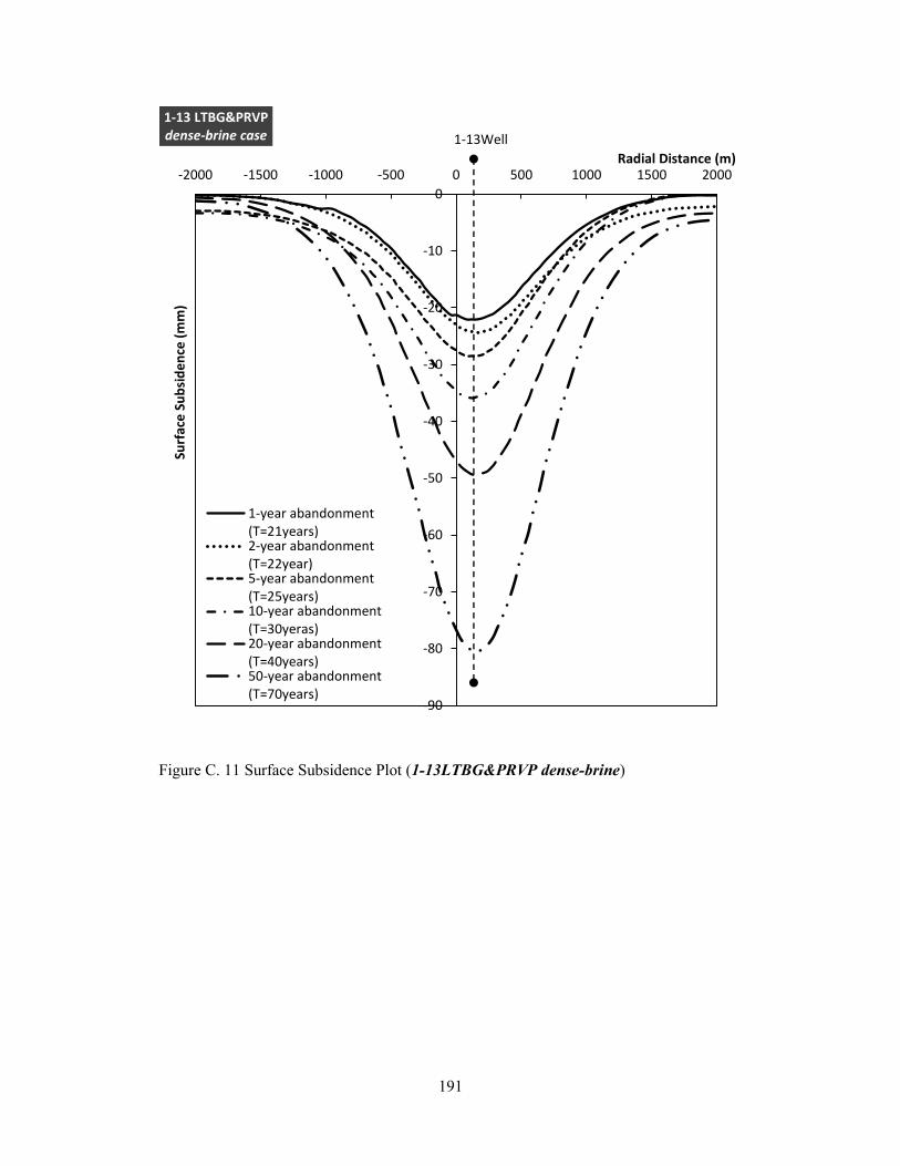
191
Figure C. 11 Surface Subsidence Plot (1-13LTBG&PRVP dense-brine)
-90
-80
-70
-60
-50
-40
-30
-20
-10
0
-2000 -1500 -1000 -500 0 500 1000 1500 2000Su
rfac
e S
ub
sid
en
ce (
mm
)
Radial Distance (m)
1-13 LTBG&PRVP dense-brine case
1-year abandonment(T=21years)2-year abandonment(T=22year)5-year abandonment(T=25years)10-year abandonment(T=30yeras)20-year abandonment(T=40years)50-year abandonment(T=70years)
1-13Well

192
Figure C. 12 Surface Subsidence Plot (1-13LTBG&PRVP dense-dense)
-50
-45
-40
-35
-30
-25
-20
-15
-10
-5
0
-2000 -1500 -1000 -500 0 500 1000 1500 2000Su
rfac
e S
ub
sid
en
ce (
mm
)
Radial Distance (m)
1-13 PRVP<BG dense-dense case
1-year abandonment(T=21years)2-year abandonment(T=22year)5-year abandonment(T=25years)10-year abandonment(T=30yeras)20-year abandonment(T=40years)50-year abandonment(T=70years)
1-13Well

193
Figure C. 13 Accumulated Casing Strains during Simulation for Cavern 1-13 LTBG
and Cavern 1-13 PRVP (1-13 LTBG&PRVP brine-brine-brine-brine)
600
700
800
900
1000
1100
1200
1300
0 0.001 0.002 0.003 0.004 0.005 0.006D
ep
th (
m)
Casing Strain of 1-13 Well (-)
1-13&8-13 LTBG&PRVP brine-brine-brine-brine case
Following Cavern 8-13 PRVPDevelopment (T=40years)
End of 50-year abandonmentSimulation (T=90years)
Cold Lake Salt
Prairie Evaporite Salt
Lotsberg Salt
Cavern 1-13 PRVP
Cavern 1-13 LTBG

194
Figure C. 14 Accumulated Casing Strains during Simulation for Cavern 8-13 LTBG
and Cavern 8-13 PRVP (1-13 LTBG&PRVP brine-brine-brine-brine)
600
700
800
900
1000
1100
1200
1300
0 0.001 0.002 0.003 0.004 0.005 0.006D
ep
th (
m)
Casing Strain of 8-13 Well (-)
1-13&8-13 LTBG&PRVP birne-brine-brine-brine case
Following Cavern 8-13 PRVPDevelopment (T=40years)
End of 50-year abandonmentSimulation (T=90years)
Cold Lake Salt
Prairie Evaporite Salt
Lotsberg Salt
Cavern 8-13 PRVP
Cavern 8-13 LTBG

195
Figure C. 15 Accumulated Casing Strains during Simulation for Cavern 1-13 LTBG
and Cavern 1-13 PRVP (1-13 LTBG&PRVP dense-dense-brine-brine)
600
700
800
900
1000
1100
1200
1300
0 0.001 0.002 0.003 0.004 0.005 0.006D
ep
th (
m)
Casing Strain of 1-13 Well (-)
1-13&8-13 LTBG&PRVP dense-dense-brine-brine case
Following Cavern 8-13 PRVPDevelopment (T=40years)
End of 50-year abandonmentSimulation (T=90years)
Cold Lake Salt
Prairie Evaporite Salt
Lotsberg Salt
Cavern 1-13 PRVP
Cavern 1-13 LTBG

196
Figure C. 16 Accumulated Casing Strains during Simulation for Cavern 8-13 LTBG
and Cavern 8-13 PRVP (1-13 LTBG&PRVP dense-dense-brine-brine)
600
700
800
900
1000
1100
1200
1300
0 0.001 0.002 0.003 0.004 0.005 0.006D
ep
th (
m)
Casing Strain of 8-13 Well (-)
1-13&8-13 LTBG&PRVP dense-dense-brine-brine case
Following Cavern 8-13 PRVPDevelopment (T=40years)
End of 50-year AbandonmentSimulation (T=90years)
Cold Lake Salt
Prairie Evaporite Salt
Lotsberg Salt
Cavern 8-13 PRVP
Cavern 8-13 LTBG

197
Figure C. 17 Accumulated Casing Strains during Simulation for Cavern 1-13 LTBG
and Cavern 1-13 PRVP (1-13 LTBG&PRVP dense-dense-dense-dense)
600
700
800
900
1000
1100
1200
1300
0 0.0005 0.001 0.0015 0.002 0.0025 0.003D
ep
th (
m)
Casing Strain of 1-13 Well (-)
1-13&8-13 LTBG&PRVP dense-dense-dense-dense case
Following Cavern 8-13 PRVPDevelopment (T=40years)
End of 50-year abandonmentSimulation (T=90years)
Cold Lake Salt
Prairie Evaporite Salt
Lotsberg Salt
Cavern 1-13 PRVP
Cavern 1-13 LTBG
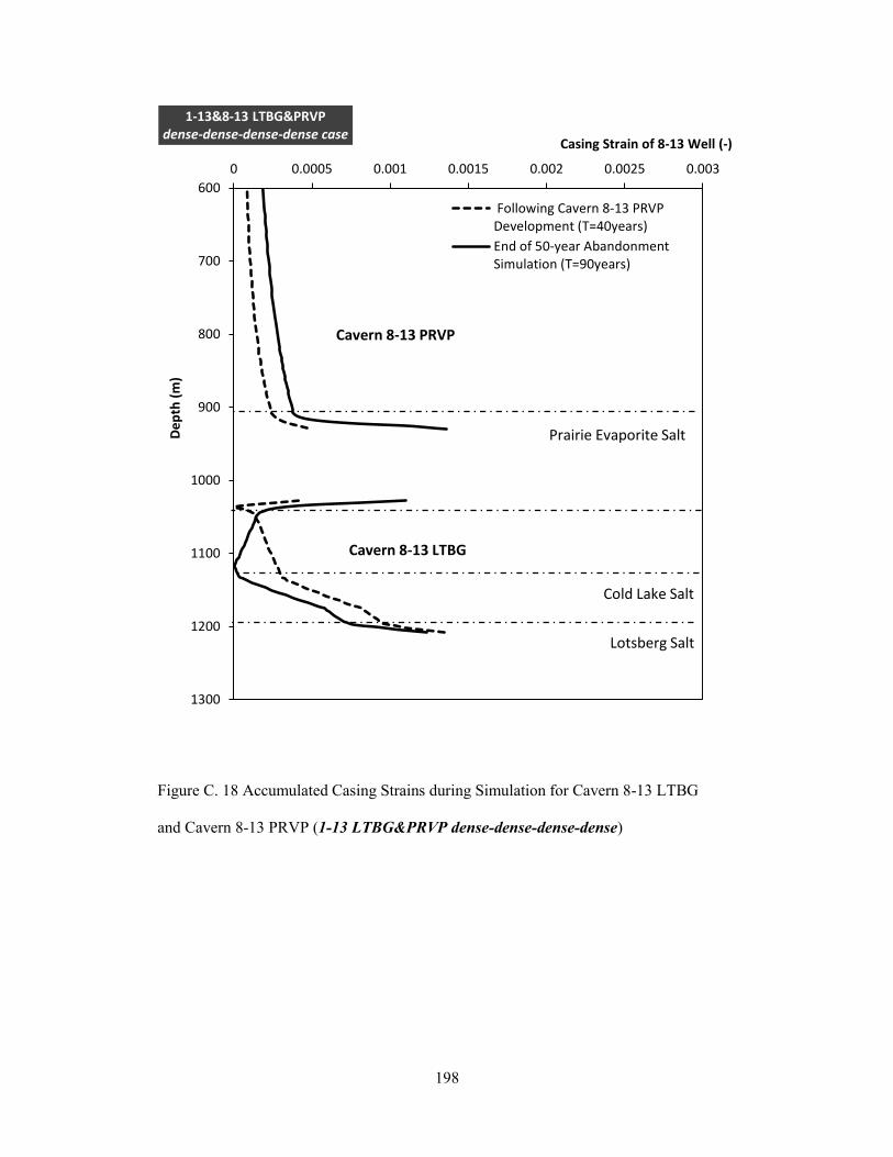
198
Figure C. 18 Accumulated Casing Strains during Simulation for Cavern 8-13 LTBG
and Cavern 8-13 PRVP (1-13 LTBG&PRVP dense-dense-dense-dense)
600
700
800
900
1000
1100
1200
1300
0 0.0005 0.001 0.0015 0.002 0.0025 0.003D
ep
th (
m)
Casing Strain of 8-13 Well (-)
1-13&8-13 LTBG&PRVP dense-dense-dense-dense case
Following Cavern 8-13 PRVPDevelopment (T=40years)
End of 50-year AbandonmentSimulation (T=90years)
Cold Lake Salt
Prairie Evaporite Salt
Lotsberg Salt
Cavern 8-13 PRVP
Cavern 8-13 LTBG

199
Figure C. 19 Surface Subsidence Plot (1-13&8-13 LTBG&PRVP brine-brine-brine-
brine)
-180
-160
-140
-120
-100
-80
-60
-40
-20
0
-2000 -1500 -1000 -500 0 500 1000 1500 2000Su
rfac
e S
ub
sid
en
ce (
mm
)
Radial Distance (m)
1-13&8-13 LTBG&PRVP brine-brine-brine-brine case
1-year abandonment(T=41years)2-year abandonment(T=42year)5-year abandonment(T=45years)10-year abandonment(T=50yeras)20-year abandonment(T=60years)50-year abandonment(T=90years)
8-13Well 1-13Well

200
Figure C. 20 Surface Subsidence Plot (1-13&8-13 LTBG&PRVP dense-brine-brine-
dense)
-160
-140
-120
-100
-80
-60
-40
-20
0
-2000 -1500 -1000 -500 0 500 1000 1500 2000Su
rfac
e S
ub
sid
en
ce (
mm
)
Radial Distance (m)
1-13&8-13 LTBG&PRVP dense-brine-brine-dense case
1-year abandonment(T=41years)2-year abandonment(T=42year)5-year abandonment(T=45years)10-year abandonment(T=50yeras)20-year abandonment(T=60years)50-year abandonment(T=90years)
8-13Well 1-13Well

201
Figure C. 21 Surface Subsidence Plot (1-13&8-13 LTBG&PRVP dense-dense-brine-
brine)
-180
-160
-140
-120
-100
-80
-60
-40
-20
0
-2000 -1500 -1000 -500 0 500 1000 1500 2000Su
rfac
e S
ub
sid
en
ce (
mm
)
Radial Distance (m)
1-13&8-13 LTBG&PRVP dense-dense-brine-brine case
1-year abandonment(T=41years)2-year abandonment(T=42year)5-year abandonment(T=45years)10-year abandonment(T=50yeras)20-year abandonment(T=60years)50-year abandonment(T=90years)
8-13Well 1-13Well
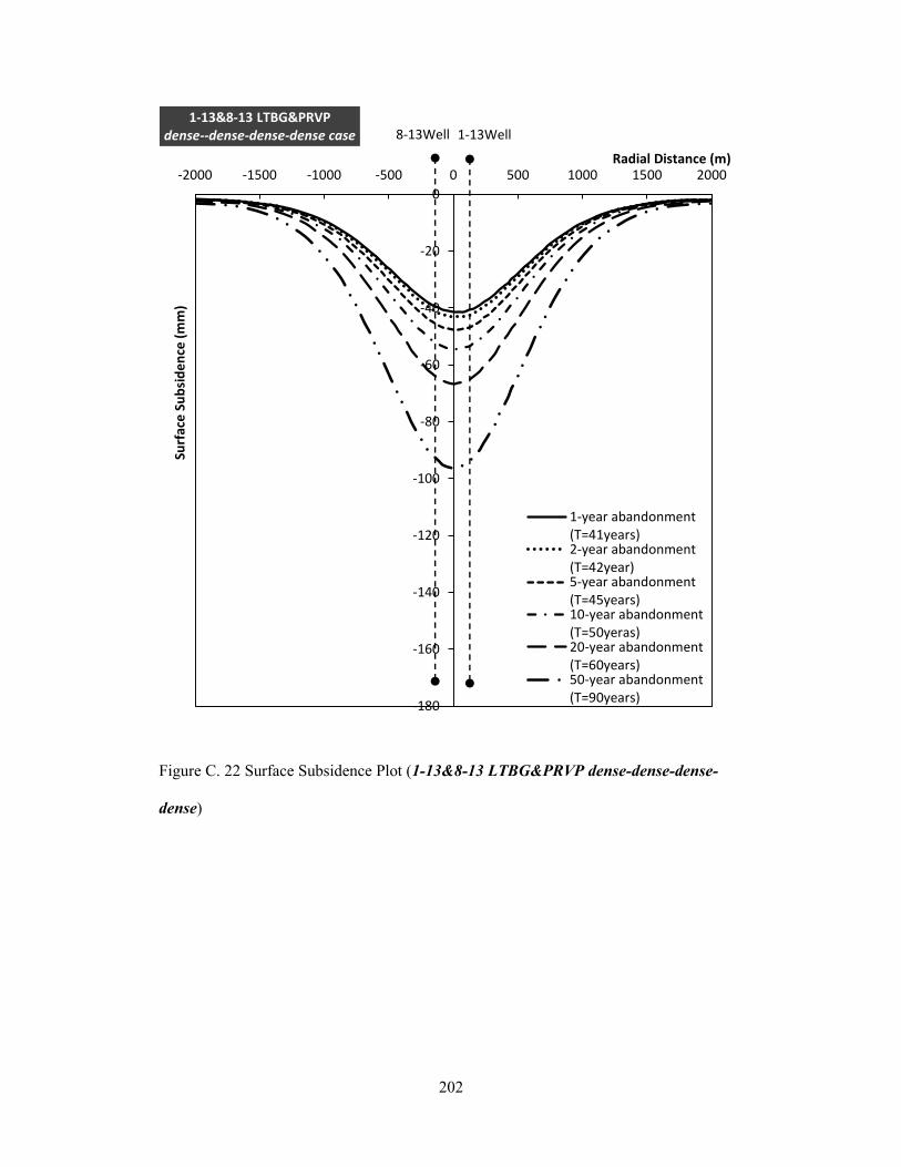
202
Figure C. 22 Surface Subsidence Plot (1-13&8-13 LTBG&PRVP dense-dense-dense-
dense)
-180
-160
-140
-120
-100
-80
-60
-40
-20
0
-2000 -1500 -1000 -500 0 500 1000 1500 2000Su
rfac
e S
ub
sid
en
ce (
mm
)
Radial Distance (m)
1-13&8-13 LTBG&PRVP dense--dense-dense-dense case
1-year abandonment(T=41years)2-year abandonment(T=42year)5-year abandonment(T=45years)10-year abandonment(T=50yeras)20-year abandonment(T=60years)50-year abandonment(T=90years)
8-13Well 1-13Well