Embed Size (px)
Citation preview

Government of India Ministry of Water Resources, River Development and Ganga Rejuvenation
CENTRAL WATER AND POWER RESEARCH STATION Pune, Maharashtra, India
Numerical Model Study of Hydrodynamics and Siltation
and Wave Tranquility Study for the Navigation of the
Dharamtar Creek (Amba River)

GOVERNMENT OF INDIA
MINISTRY OF WATER RESOURCES
CENTRAL WATER AND POWER RESEARCH STATION
PUNE 411 024, INDIA
NUMERICAL MODEL STUDY REPORT
March 2015
Numerical Model Study of Hydrodynamics and Siltation
and Wave Tranquility Study for the Navigation of the
Dharamtar Creek (Amba River)

JSW Dharamtar Port Pvt. Limited March 2015
Numerical Model Study of Hydrodynamics and Siltation and Wave Tranquility Study for the Navigation of the Dharamtar Creek (Amba River)

Mathematical Modelling Report i JSW Dharamtar Port Pvt. Limited
Contents
1 Introduction ................................................................................................................................... 10
1.1 Background .................................................................................................................................. 10
1.2 The project ................................................................................................................................... 12
1.3 Summary of Terms of Reference ................................................................................................. 14
1.4 Intent of the report ........................................................................................................................ 14
1.5 Format of the report ..................................................................................................................... 14
2 Site Condition ............................................................................................................................... 15
2.1 Geographical Location ................................................................................................................. 15
2.2 Meteorological and Oceanographic Conditions ........................................................................... 16
2.2.1 Temperature ................................................................................................................................. 16
2.2.2 Rainfall ......................................................................................................................................... 16
2.2.3 Relative Humidity ......................................................................................................................... 16
2.2.4 Wind ............................................................................................................................................. 17
2.2.5 Wave Climate ............................................................................................................................... 18
2.2.6 Tides ............................................................................................................................................. 21
2.2.7 Currents ........................................................................................................................................ 21
3 Site Investigations ........................................................................................................................ 22
3.1 General ......................................................................................................................................... 22
3.2 Bathymetric Survey ...................................................................................................................... 22
3.3 Tidal Data ..................................................................................................................................... 22
3.4 Current ......................................................................................................................................... 22
3.5 Temperature ................................................................................................................................. 26
3.6 Salinity and Total Suspended Solid ............................................................................................. 27
3.7 Bed Samples ................................................................................................................................ 30
4 Numerical Simulations ................................................................................................................. 32
4.1 General ......................................................................................................................................... 32
4.2 MIKE 3 FM ................................................................................................................................... 33
4.3 MIKE 21 FM - Regional Model Setup .......................................................................................... 35
4.3.1 General ......................................................................................................................................... 35
4.3.2 Bathymetry ................................................................................................................................... 35

Mathematical Modelling Report ii JSW Dharamtar Port Pvt. Limited
4.3.3 Tidal data (Boundary) ................................................................................................................... 36
4.3.4 Model Set up ................................................................................................................................ 38
4.3.5 Regional Model Calibration .......................................................................................................... 38
4.3.6 Regional Model Results ............................................................................................................... 41
4.4 MIKE 21 FM – Local Model Set-up for Existing Conditions ......................................................... 44
4.4.1 Model Set Up................................................................................................................................ 44
4.4.2 Bathymetry ................................................................................................................................... 44
4.4.3 Flow Hydrodynamics .................................................................................................................... 46
4.4.4 Sedimentation Model – MIKE 21 MT ........................................................................................... 51
4.4.5 Model Set up – MIKE 21 MT ........................................................................................................ 52
5.4.5 Wave tranquillity ........................................................................................................................... 54
5.4.6 Shoreline Evolution due to Construction ...................................................................................... 54
4.5 Disposal of the Dredged sediments ............................................................................................. 54
5 Conclusions and Recommendations ........................................................................................... 55
5.1 Conclusions .................................................................................................................................. 55
5.2 Recommendations ....................................................................................................................... 55

Mathematical Modelling Report i JSW Dharamtar Port Pvt. Limited
Tables
Table 3-1: Grain size distribution of the collected samples (in % of dry weight) ...... 31
Table 4-1: Details of Model Set Up .......................................................................... 38
Table 4-2: Details of Model Set Up .......................................................................... 44
Table 4-3: Parameters applied in the model simulations ......................................... 53
Table 4-4: Concentration applied during non-monsoon and monsoon period ......... 53

Mathematical Modelling Report ii JSW Dharamtar Port Pvt. Limited
Figures
Figure 1-1: Location of the Dolvi facility on the Map of India (top) and on the map
of Maharashtra (bottom) ......................................................................... 11
Figure 1-2: The existing barge berthing facility at Dharamtar ................................... 12
Figure 2-1: Location of the proposed Facility in side Dharamtar Creek .................... 15
Figure 2-2: Location of the proposed Existing waterfront and Steel plant Facility in
side Dharamtar Creek ............................................................................. 16
Figure 2-3: Wind rose diagram (Source: IMD, 1976 – 2015). .................................. 17
Figure 2-4: Cumulative frequency graph for the wind speed (Source: IMD, 1976 –
2015). ...................................................................................................... 17
Figure 2-5: Wave height rose diagram Offshore (IMD, 1976 – 2015). ...................... 19
Figure 2-6: Cumulative frequency graph for wave height (Source: IMD, 1976 –
2015). ...................................................................................................... 20
Figure 2-7: Wave period rose diagram Offshore (IMD, 1976 – 2015). ...................... 20
Figure 3-1: Bathymetry chart of the area – MMB survey ........................................... 23
Figure 3-2: Tidal Levels at the Dharamtar Jetty ........................................................ 24
Figure 3-3: Location of the Current Measurements .................................................. 24
Figure 3-4: Current plots of stations 1 to 5 in sequence ........................................... 25
Figure 3-5: Current plots of stations 1 to 5 in sequence ........................................... 26
Figure 3-6: Locations of monitoring stations for salinity and TSS ............................. 28
Figure 3-7: Salinity and TSS profile at Station 1 ....................................................... 28

Mathematical Modelling Report iii JSW Dharamtar Port Pvt. Limited
Figure 3-8: Salinity and TSS profile at Station 2 ....................................................... 29
Figure 3-8: Salinity and TSS profile at Station 3 ....................................................... 29
Figure 3-8: Locations of Bed Samples collected in the Dharamtar Creek ................ 30
Figure 4-1: Extents of the global model, showing tidal station of C-Map .................. 35
Figure 4-2: Flexible mesh showing the Model Domain of the Model ........................ 36
Figure 4-3: Tidal Levels on the Nothern Boundary ................................................... 37
Figure 4-4: Tidal Levels on the Southern Boundary .................................................. 37
Figure 4-5: Disacharge Boundary data for the up-stream Amba River boundary ..... 38
Figure 4-6: Calibration plot showing measured and predicted current speed (top)
and direction (bottom) at Station 1 .......................................................... 39
Figure 4-7: Calibration plot showing measured and predicted current speed (top)
and direction (bottom) at Station 3 .......................................................... 39
Figure 4-6: Calibration plot showing measured and predicted current speed (top)
and direction (bottom) at Station 4 .......................................................... 40
Figure 4-9: Calibration plot showing measured and predicted current speed (top)
and direction (bottom) at Station 5 .......................................................... 41
Figure 4-10: Flood Current Vectors ............................................................................. 42
Figure 4-11: Ebb Current Vectors ............................................................................... 43
Figure 4-12: Profile series extarcted from the global model for the Local model
boundary ................................................................................................. 44
Figure 4-13: Local Bathymetry (finite Mesh) for the Model Simulation ....................... 45
Figure 4-14: Local Bathymetry (finite Mesh) – close up for the Model Simulation ...... 46

Mathematical Modelling Report iv JSW Dharamtar Port Pvt. Limited
Figure 4-15: Local Bathymetry (finite Mesh) – close up for the Model Simulation –
With Reclamation .................................................................................... 46
Figure 4-16: Current speed in the Local Model under Flood tide ................................ 47
Figure 4-17: Current speed in the Local Model under Ebb tide .................................. 48
Figure 4-18: Current speed in the Local Model under Flood tide – With reclamation . 49
Figure 4-19: Current speed in the Local Model under Ebb tide – With reclamation.... 50
Figure 4-20: Extracted Current Speed at location t1 and t2 – Without reclamation -
Flood tide ................................................................................................ 51
Figure 4-20: Extracted Current Speed at location t1 and t2 – With reclamation -
Flood tide ................................................................................................ 51

Mathematical Modelling Report v JSW Dharamtar Port Pvt. Limited
SYMBOLS AND ABBREVIATIONS
Symbols and abbreviations used are generally in accordance with the following list.
1 Proper names and organisations - India
BIS .................... Bureau of Indian Standards
GAIL… ………..Gas Authority of India
IAPH.................The International Association of Ports and Harbours
MMB…………….Maharashtra Maritime Board
MCZMA ........... Maharashtra Coastal Zone Management Authority
MIDC ................ Maharashtra Industrial Development Corporation
MLDB ............... Main Lighting Distribution Board
MoEF ................ Ministry of Environment and Forests
MoS .................. Ministry of Shipping
MPCB ............... Maharashtra Pollution Control Board
MSEDCL .......... Maharashtra State Electricity Distribution Company Limited
NHO ................. National Hydro graphic Office, Dehra Dun
OCIMF..............The Oil Companies International Marine Forum
PINAC .............. Permanent International Association of Navigation Congress
SIGTTO.............Society of International Gas Tankers & Terminal Operators Ltd.
SoI………………Survey of India
2 Proper names and organisations – Other
BA ..................... British Admiralty
BR .................... Beckett Rankine

Mathematical Modelling Report vi JSW Dharamtar Port Pvt. Limited
BS ..................... British Standard
IMO ................... International Maritime Organization
ISPS ................. International Ship and Port facility Security code
UTM.................. Universal Transverse Mercator (map projection)
WGS ................. World Geodetic System (ellipsoid for map projection)
3 Other abbreviations
Approx. ............. approximately
cif ...................... cost, insurance, freight
dia ..................... diameter
feu .................... forty foot equivalent unit (container)
fob .................... free on board
max ................... maximum
min .................... minimum
No ..................... number (order) as in No 6
nr ...................... number (units) as in 6 nr
Panamax .......... ship of max permissible beam of 32.2m for transiting the Panama
Canal
ppt .................... parts per thousand
teu .................... twenty-foot equivalent unit (container)
BOOT ............... Build – Own - Operate – Transfer
CCTV................ Closed Circuit Television
CSR .................. Corporate Social Responsibility
CBRM………….Coal bearing raw material

Mathematical Modelling Report vii JSW Dharamtar Port Pvt. Limited
DPR .................. Detailed Project Report
EIA .................... Environmental Impact Assessment
HAT .................. Highest Astronomical Tide
MHWS .............. Mean High Water Spring tides
MHS……………Material Handling System
MSL .................. Mean Sea Level
MLWS............... Mean Low Water Spring tides
LAT ................... Lowest Astronomical Tide
CD .................... Chart Datum
ICD ................... Inland Container Depot
IT ...................... Information Technology
IBRM…………..Iron bearing raw material
LOA .................. Length overall (of a ship)
LCL ................... Less Than Container Load / Consolidation Containers
M ...................... “mega” or one million (106)
MVA……………Mega volt ampere
MoU .................. Memorandum of Understanding
SEZ .................. Special Economic Zone
ToR ................... Terms of Reference
VTMS ............... Vessel Traffic Management System
4 Units of measurement
Length, area and volume
mm ................... millimetre(s)

Mathematical Modelling Report viii JSW Dharamtar Port Pvt. Limited
m ...................... metre(s)
km ..................... kilometre(s)
n. mile ............... nautical mile(s)
mm2 .................. square millimetre(s)
m2 ..................... square metre(s)
km2 ................... square kilometre(s)
ha ..................... hectare(s)
m3 ..................... cubic metre(s)
Time and time derived units
s ........................ second(s)
min .................... minute(s)
h ....................... hour(s)
d ....................... day(s)
wk ..................... week(s)
mth ................... month(s)
yr ...................... year(s)
mm/s................. millimetres per second
km/h.................. kilometres per hour
m/s .................... metres per second
knot................... nautical mile per hour
Mass, force and derived units
kg ...................... kilogram(s)
g ....................... gram = kg x 10-3

Mathematical Modelling Report ix JSW Dharamtar Port Pvt. Limited
t ........................ tonne = kg x 103
displacement .... the total mass of the vessel and its contents. (This is equal to the
volume of water displaced by the vessel multiplied by the density of the
water.)
DWT ................. dead weight tonne, the total mass of cargo, stores, fuels, crew and
reserves with which a vessel is laden when submerged to the summer
loading line. (Although this represents the load carrying capacity of the
vessel it is not an exact measure of the cargo load).
Mt ..................... million tonnes = t x 106
TPD...................Tonnes per day
TPH/tph.............Tonnes per hour
Other units
°C ..................... degrees Celsius (temperature)
Mtpa ................. million tons per annum
Mathematical Modelling Report 10 JSW Dharamtar Port Pvt. Limited
1 Introduction
1.1 Background
JSW Group is one of the fastest growing business conglomerates with a strong presence
in the core economic sector. This Mr. Sajjan Jindal led enterprise has grown from a steel
rolling mill in 1982 to a multi business conglomerate worth US $ 11 billion within a short
span of time. As part of the US $ 16.5 billion O. P. Jindal Group, JSW Group has
diversified interests in Steel, Energy, Minerals and Mining, Aluminium, Infrastructure,
Cement and Information Technology.
JSW Group has grown significantly over the years and taking steps for rapid expansion to
ramp up the capacity of Vijaynagar Steel Plant in Karnataka from the present 10 MTPA to
12 MTPA by the year 2014. In addition, JSW Energy Limited, a JSW Group company, is
the first independent Power producer to set up 2 units of 130 MW each and 4 units of 300
MW each and producing power using Corex gas and coal.
The JSW group owns and operates JSW Steel Limited, Dolvi Works, a 3.2 Million tons per
annum (Mtpa) Steel plant based at Dolvi, Maharashtra working on BF-DR-CONARC-CSP
process. The plant also has facilities for cold rolling, galvanizing, colour coating,
galvalume, and supplements the pipe and tube plant at Kalmeshwar, Nagpur in the state
of Maharashtra.
The JSW Infrastructure Ltd (JSWIL) is a JSW Group company which is presently into
design, finance, development, operation and maintenance of ports, rail/road and inland
water connectivity, development of port based SEZ and other related infrastructure
developments works along with terminal handling operations and port management. The
JSWIL has constructed a mega port in Jaigarh, near Ratnagiri, in Maharashtra, with a
present capacity of 15 Mtpa through a Special Purpose Vehicle (SPV) presently under
expansion to 50 Mtpa. Another Subsidiary of JSWIL, the South West Port Limited (SWPL),
has developed berth number 5A and 6A in the Mormugao Port Trust on BOOT basis and
has successfully handled more than 50 million cargos in about 9 years.
JSW Dharamtar Port Limited (JSWDPL) is a SPV under the aegis of JSWIL, to handle the
proposed EXIM cargo of the JSW Steel Limited, Dolvi works. The Plant was taken over
from the erstwhile M/s Ispat Industries Limited, in the Year 2011. The Steel plant has
unique distinction of having road, rail and water connectivity. It is located on the right bank
of the Amba River, which falls in to the Dharamtar Creek, before merging in to the Arabian
Sea. There is a barge handling facility which mostly handles raw materials for the Steel
Plant. The location of the JSW Steel Limited, Dolvi works is shown in Figure 1.1 below.

Mathematical Modelling Report 11 JSW Dharamtar Port Pvt. Limited
Figure 1-1: Location of the Dolvi facility on the Map of India (top) and on
the map of Maharashtra (bottom)
The cargo in the fair season, is handled at the Mumbai outer anchorage (mostly in the
Bravo anchorage), and then transported through barges to the Jetty at Dharamtar,
near Dolvi. The berthing facility consists of 430 m barge berth with two approaches as
shown in Figure 1.2. The berth is equipped with two barge unloaders and two LHM
250 Leibherr Cranes.

Mathematical Modelling Report 12 JSW Dharamtar Port Pvt. Limited
Figure 1-2: The existing barge berthing facility at Dharamtar
1.2 The project
Modern day industry requires a larger market and economical transportation systems to
get its input or base materials at lowest costs and the finished products are disposed at
many destinations at a comparative cost. To achieve this, appropriate transportation
facilities are very essential. Thus, such propositions are possible only if such industries are
set up as near as possible to a seaport.
The existing berthing facility at Dharamtar is for handling of barges. Originally designed for
barge sizes of 2500 DWT, presently barges up to 3700 DWT are handled at the berth.
There are 4 berths (Berth no 1 to 4) totaling to about 331.5 m in one alignment. Berth no. 5
of about 100 m long, is at an angle of 30. The berth structure is designed on pile
foundations and has a concrete RCC decking. The berth is provided with two approaches,
which apart from providing access to the berths carry the conveyor systems as well.
The present logistical chain for the Dharamtar facility is fairly simple. The mother vessels
are handled at the anchorage and load the barges using ship’s gear. The barges then
move in to the creek and travel to the berth and gets unloaded. The empty barges are
serviced and start their journey back to the anchorage for re-loading. Typically this is the
fair weather operation, which spans 8 months in year. At this outer anchorage there are no
depth restrictions and therefore, vessels up to cape size ships could call in. The ships do
Mathematical Modelling Report 13 JSW Dharamtar Port Pvt. Limited
move shoreward during the midstream handling as they lighten themselves. This
effectively reduces the distance of travel of the barges travel, resulting in savings in fuel
and time of travel.
In the monsoon season, due to the wave disturbance in the outer anchorage, the action of
cargo transfer shifts to the inner anchorage. In such a scenario, due to the depth
limitations in the inner anchorage, mother vessels up to 40,000 DWT only could be
serviced. The vessels generally come partially loaded to be handled inside the inner
anchorage. The inner anchorage provides the necessary tranquility for cargo handling.
However, it must be understood that the number of inner anchorages are limited. About 5
anchorages are being developed by the Mumbai Port Trust. Though additional anchorages
could be developed, but the efficiency would be low.
Therefore, with the increase in the cargo volumes, the dependencies on the inner
anchorages should be reduced proportionately. There are two inherent inadequacies
ingrained in the inner anchorage operations.
1. Handling of vessel sizes limited to 40000 DWT. Hence the freight charges
increases.
2. Since the numbers of anchorages are limited, as the number of ships to be handled
increase, the waiting time also increase.
Accordingly, in order to reduce redundancies and uncertainties in the system it was
decided to do away with the inner anchorage for the planning of the cargo movement in
the Phase II and Phase III. Instead the cargo could be shifted and handled from Jaigarh
Port, where the turnaround of the ship would be much higher.
In the report (as in the Logistic studies), the fair weather cargo is considered to be handled
from the outer anchorage and the monsoon cargo from the Jaigarh Port. In another
scenario the entire cargo is being handled from the Jaigarh Port. The logistic study is dealt
in a separate report; the present report would only deal with the Mathematical model
studies as part of compliance for the construction and expansion of the water front
structures for handling the increased cargo volumes.

Mathematical Modelling Report 14 JSW Dharamtar Port Pvt. Limited
1.3 Summary of Terms of Reference
The broad scope of work for the mathematical model study report would include the
following:
Review of the existing reports, available data and documents
Data collection and collation
Mathematical model studies
Discussion of the Results
1.4 Intent of the report
The purpose of this report is to determine the impact of the waterfront development in
order to handle the enhanced cargo volumes.
The report would discuss the siltation and the morphological changes in the creek as well.
1.5 Format of the report
The report is arranged as below:
Chapter 1: Introduction
Chapter 2: Site Condition
Chapter 3: Field Investigations
Chapter 4: Model Set up
Chapter 5: Conclusions and Recommendations

Mathematical Modelling Report 15 JSW Dharamtar Port Pvt. Limited
2 Site Condition
2.1 Geographical Location
The location of Dharamtar Creek and Karanja Creek along the west coast of India, and
proposed Thermal Power Plant (TPP) are shown in Figure 2.1. The location of the
proposed TPP lies between latitudes 180 43’ to 180 45’ North and 720 58’ to 720 59’ East
as shown in Figure 2.2. The general topography of the area is flat terrain surrounded by
creeks on three sides.
Figure 2-1: Location of the proposed Facility in side Dharamtar Creek

Mathematical Modelling Report 16 JSW Dharamtar Port Pvt. Limited
Figure 2-2: Location of the proposed Existing waterfront and Steel plant
Facility in side Dharamtar Creek
2.2 Meteorological and Oceanographic Conditions
2.2.1 Temperature
The mean of the highest air temperature recorded at Mumbai is 350 C in the months of
April and May while the mean lowest is 160 C recorded in the month of January. Mean
daily maximum and minimum temperatures are 340 C and 220 C respectively.
2.2.2 Rainfall
The average yearly rainfall is about 2098 mm, of which 1965 mm (93.66%) occur during
June to September. Usually maximum average monthly rainfall of 709 mm occurs in July.
There is practically no rainfall from December to April.
2.2.3 Relative Humidity
Mean yearly relative humidity at 0830 hours is 77% while the same at 1730 hours is 71%.
The monthly average is lowest in February (62%) and highest in July to September (85%).

Mathematical Modelling Report 17 JSW Dharamtar Port Pvt. Limited
2.2.4 Wind
Ship observed offshore wind data for a period of 35 years from 1976 to 2015 were
obtained from the India Meteorological Department (IMD) and analysed for the grid
covering Lat. 18o - 20o N and Long 71o - 73o E, which centers the area of interest. The
distribution of wind speed and direction is presented in Figure 2.3. The observations
represent measurements taken at sea level for 3 minutes. It may be seen that west is the
predominant direction and that the wind speed is less than 10 m/s for 88% of the time as
shown in figure 2.4.
It was observed that the predominant wind is NE-N-NW in January. It gradually shifts
towards west and by May it becomes NW to SW. During the months of June, July and
August, the wind blows from W to SW. From September the wind direction starts changing
and by December, again the predominant sector becomes NE-N-NW.
Figure 2-3: Wind rose diagram (Source: IMD, 1976 – 2015).
Figure 2-4: Cumulative frequency graph for the wind speed (Source: IMD,
1976 – 2015).

Mathematical Modelling Report 18 JSW Dharamtar Port Pvt. Limited
0
10
20
30
40
50
60
70
80
90
100
0 5 10 15 20 25 30 35 40
Percentage
Wind Speed (m/s)
Cumulative Frequency - Wind Speed
It may be observed that during the fair weather season viz. October to May, the wind
speed is less than 6 m/s for about 91% of the time. However, during the monsoon season
(June to September), the wind speed is less than 8 m/s knots for only 62% of the time. It
may also be seen that during the peak monsoon period (July and August), wind speed of 6
to 13 m/s occurs for about 29% of the time. Wind speed of 13 m/s knots is seldom
exceeded.
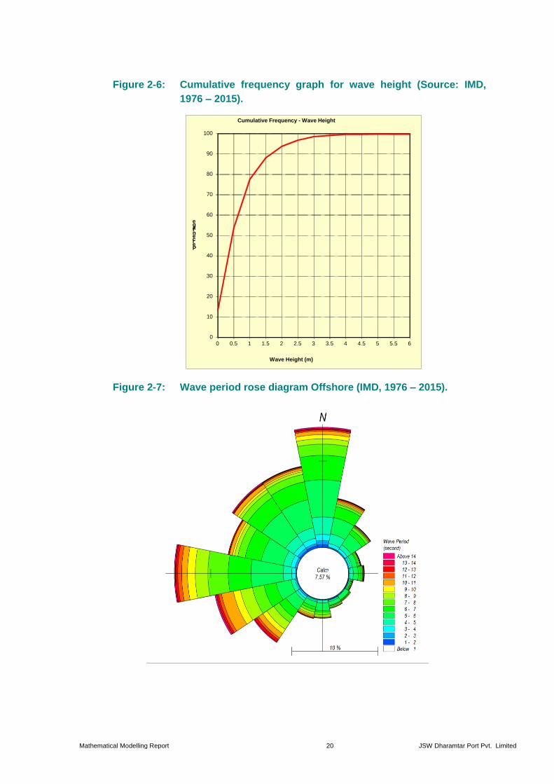
2.2.5 Wave Climate
The ship observed wave data were collected from the India Meteorological Department
(IMD) for the quadrant bounded by Latitudes 18o to 20o N and Longitudes 71o to 73o E,
between 1976 and 2005. The annual distribution of wave heights is given in the form of
wave rose diagrams in Figures 2.5. It may be seen that the predominant directions of
waves in the deep sea are from SW to NW. It can also be seen that waves are less than 1
m, 2 m and 3 m in height for 77, 94 and 98% of the time respectively as may be observed
from the cumulative frequency curve given as Figure 2.6. Figure 2.7 shows the wave rose
for wave period.

Mathematical Modelling Report 19 JSW Dharamtar Port Pvt. Limited
During the pre-monsoon period (January to May) over 92.93% of waves are less than 3 m
in height. During the monsoon period (June to September) wave heights are less than 2 m
for 85 % and less than 3 m for 97% of the time. During the post monsoon period (October
to December) wave heights are more than 3 m for 0.9% of the time. The predominant
wave directions are in the NW quadrant for pre-monsoon period, from W to SW during the
southwest monsoon and from NE to NW in the post-monsoon period. These wave heights
applicable for the offshore conditions and wave are completely attenuated as they enter
the well-protected creek.
Figure 2-5: Wave height rose diagram Offshore (IMD, 1976 – 2015).
Mathematical Modelling Report 20 JSW Dharamtar Port Pvt. Limited
Figure 2-6: Cumulative frequency graph for wave height (Source: IMD,
1976 – 2015).
0
10
20
30
40
50
60
70
80
90
100
0 0.5 1 1.5 2 2.5 3 3.5 4 4.5 5 5.5 6
Percentage
Wave Height (m)
Cumulative Frequency - Wave Height
Figure 2-7: Wave period rose diagram Offshore (IMD, 1976 – 2015).

Mathematical Modelling Report 21 JSW Dharamtar Port Pvt. Limited
2.2.6 Tides
The tides in the Mumbai region are of the semi-diurnal type, i.e., characterized by
occurrence of two high and two low waters every day. There is a marked inequality in the
levels of the two low waters in a day. The important tidal datum planes with respect to
Chart Datum at Apollo Bandar (Latitude 180 55’ N, Longitude 720 50’ E) are as under.
MHWS + 4.4 m
MHWN + 3.3 m
MSL + 2.5 m
MLWN + 1.9 m
MLWS + 0.8 m
It may be mentioned that the tidal levels mentioned above get modified, albeit to a minor
extent, by coastal geometry and configuration at the proposed port site.
2.2.7 Currents
The currents in the Mumbai region in the near shore zone are tide induced with reversal at
high and low waters. The current speeds are of the order of 0.75 m/s to 1.5 m/s (1.5 to 3
Knots).

Mathematical Modelling Report 22 JSW Dharamtar Port Pvt. Limited
3 Site Investigations
3.1 General
The site investigations were carried out for collecting field data with regard to, bathymetry
of the area, tidal levels, current, temperature, salinity and total suspended solids (TSS)
specific to the area under consideration. The collected data is used both as input to the
mathematical model as well as for calibration.
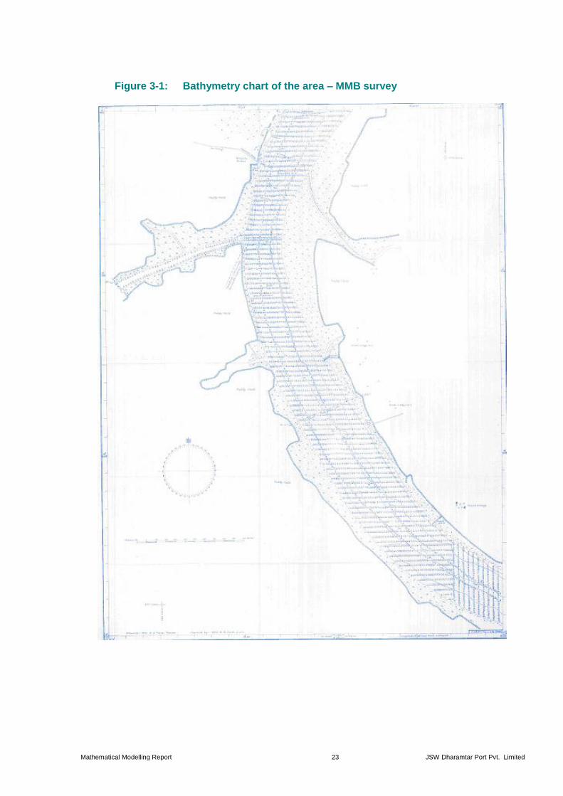
3.2 Bathymetric Survey
Bathymetric survey was conducted by Mumbai Maritime Board (MMB) of the area as
shown in figure 3.1and the levels were reduced to chart datum. This was used as the
basic bathymetry for the model and calculation of the dredging quantities.
3.3 Tidal Data
Tidal data was collected at the Dharamtar Jetty. The zero of the tide pole was connected
to the Bench Mark by levelling. The observations after tide is reduced to chart datum are
given as Figure 3.2.
It can be seen that the maximum tide is 5.45 m and tidal range is 5 m. This tide will be
used at the lower boundary defining the flow of the creek near Dharamtar Jetty.
3.4 Current
Current data was collected at 5 locations as shown in Figure 3.3. The time series of
current speed are plotted and given in Figure 3.4.
Mathematical Modelling Report 23 JSW Dharamtar Port Pvt. Limited
Figure 3-1: Bathymetry chart of the area – MMB survey

Mathematical Modelling Report 24 JSW Dharamtar Port Pvt. Limited
Figure 3-2: Tidal Levels at the Dharamtar Jetty
Figure 3-3: Location of the Current Measurements

Mathematical Modelling Report 25 JSW Dharamtar Port Pvt. Limited
Figure 3-4: Current plots of stations 1 to 5 in sequence
Mathematical Modelling Report 26 JSW Dharamtar Port Pvt. Limited
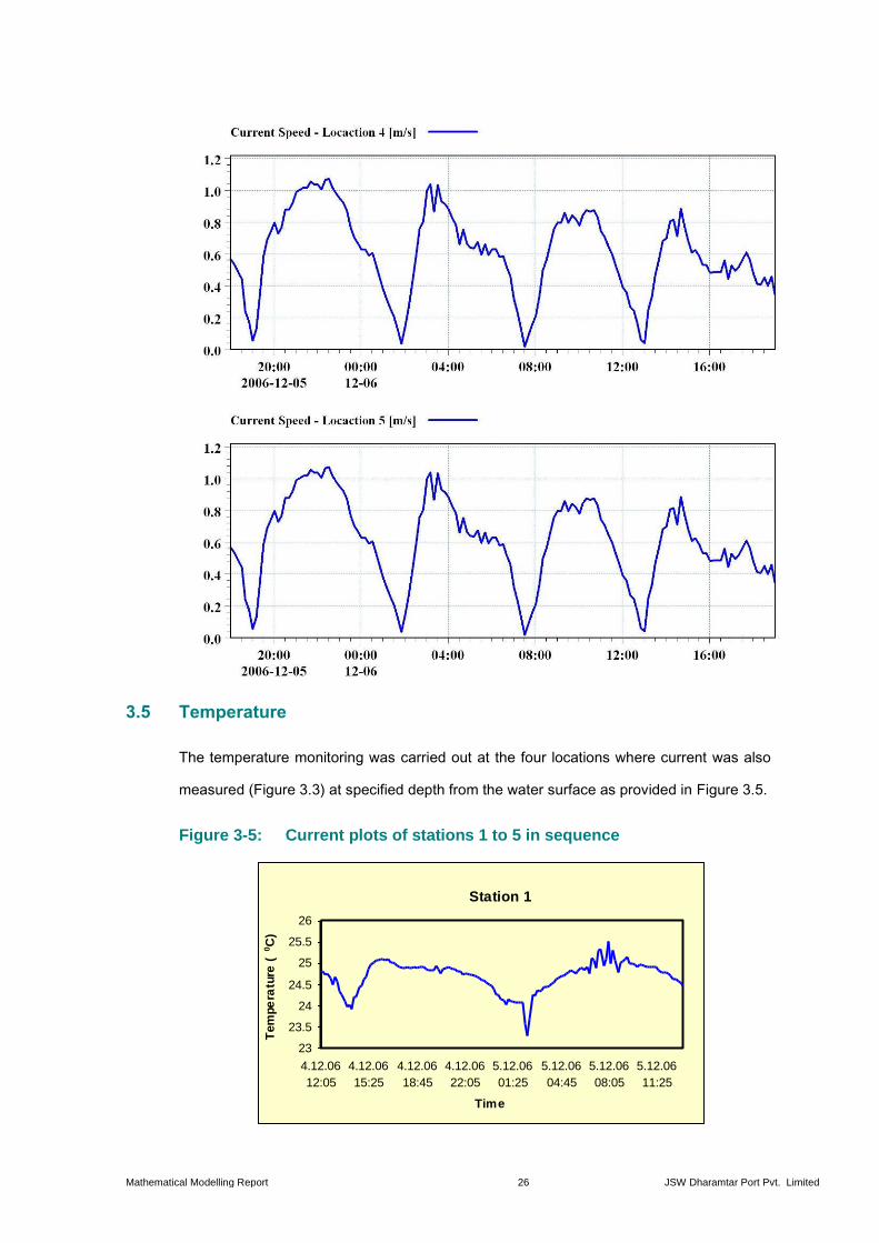
3.5 Temperature
The temperature monitoring was carried out at the four locations where current was also
measured (Figure 3.3) at specified depth from the water surface as provided in Figure 3.5.
Figure 3-5: Current plots of stations 1 to 5 in sequence
Station 1
23
23.5
24
24.5
25
25.5
26
4.12.06
12:05
4.12.06
15:25
4.12.06
18:45
4.12.06
22:05
5.12.06
01:25
5.12.06
04:45
5.12.06
08:05
5.12.06
11:25
Time
Tem
pe
ratu
re (
0C
)

Mathematical Modelling Report 27 JSW Dharamtar Port Pvt. Limited
3.6 Salinity and Total Suspended Solid
The water samples were analysed by MMB using CTD meter for the TSS and the salinity
of the creek at three locations as depicted in Figure 3.6. The salinity and TSS profiles of
the above said locations are given in Figure 3.7 to 3.9.

Mathematical Modelling Report 28 JSW Dharamtar Port Pvt. Limited
Figure 3-6: Locations of monitoring stations for salinity and TSS
Figure 3-7: Salinity and TSS profile at Station 1
Salinity Profile at Station 1
26
27
28
29
30
31
32
33
34
4.12.06
12:05
4.12.06
13:55
4.12.06
18:25
4.12.06
20:25
5.12.06
1:20
5.12.06
3:20
5.12.06
7:20
5.12.06
9:20
Time
Sali
nit
y (
%)
0.2 m from the Top 0.4 m from the Top 0.6 m from the Top
TSS Profile at Station 1
0
100
200
300
400
500
600
700
800
900
4.12.06
12:05
4.12.06
13:55
4.12.06
18:25
4.12.06
20:25
5.12.06
1:20
5.12.06
3:20
5.12.06
7:20
5.12.06
9:20
Time
TS
S (
mg
/l)
0.2 m from the Top 0.4 m from the Top 0.6 m from the Top

Mathematical Modelling Report 29 JSW Dharamtar Port Pvt. Limited
Figure 3-8: Salinity and TSS profile at Station 2
Salinity Profile at Station 2
242526272829303132
3.12.06
11:10
3.12.06
13:10
3.12.06
17:35
3.12.06
19:35
3.12.06
00:25
4.12.06
2:25
4.12.06
6:25
4.12.06
8:25
Time
Sa
lin
ity (
%)
0.2 m from the Top 0.4 m from the Top 0.6 m from the Top
TSS Profile at Station 2
0
100
200
300
400
500
600
700
3.12.06
11:10
3.12.06
13:10
3.12.06
17:35
3.12.06
19:35
3.12.06
00:25
4.12.06
2:25
4.12.06
6:25
4.12.06
8:25
Time
TS
S (
mg
/l)
0.2 m from the Top 0.4 m from the Top 0.6 m from the Top
Figure 3-9: Salinity and TSS profile at Station 3
Salinity Profile at Station 3
23
2425
26
27
2829
30
2.12.06
10:25
2.12.06
12:25
2.12.06
16:55
2.12.06
18:55
2.12.06
23:50
3.12.06
1:50
3.12.06
5:30
Time
Sali
nit
y (
%)
0.2 m from the Top 0.4 m from the Top 0.6 m from the Top

Mathematical Modelling Report 30 JSW Dharamtar Port Pvt. Limited
TSS Profile at Station 3
0
100
200
300
400
500
600
2.12.06
10:25
2.12.06
12:25
2.12.06
16:55
2.12.06
18:55
2.12.06
23:50
3.12.06
1:50
3.12.06
5:30
Time
TS
S (
mg
/l)
0.2 m from the Top 0.4 m from the Top 0.6 m from the Top
3.7 Bed Samples
The grain size distribution analysis was carried out at three locations as shown in figure
3.9 3.1, presents the description of the analysis. The texture of bed material at location 1,
which is closest and most relevant to the site, is clayey with very little sand. But as one
moves towards the Dharamtar creeks mouth the percentage of sand content increases
because of its vicinity from the sea.
Figure 3-10: Locations of Bed Samples collected in the Dharamtar Creek

Mathematical Modelling Report 31 JSW Dharamtar Port Pvt. Limited
Table 3-1: Grain size distribution of the collected samples (in % of dry
weight)
Locations Sand Silt Clay Texture
1 14.90 2.10 83.00 Clayey
2 35.50 3.70 60.80 Clayey
3 35.00 58.00 7.00 Silty

Mathematical Modelling Report 32 JSW Dharamtar Port Pvt. Limited
4 Numerical Simulations
4.1 General
Cooling system is a part of the proposed power plant. This system includes an intake,
which supplies cold water to the power plant, used for cooling the condensers. The
resulting warm water is then collected and discharged through a suitably designed outfall.
Understanding of hot water dispersion in the system is essential for two reasons. Firstly, it
should be ascertained that rise in ambient water temperature should not be more than the
standards given by MoEF to safeguard marine life and environment. Secondly because
the flow dynamics of the area results in the mixing of the warm water with the water near
the intake and if this water is permitted, the efficiency of the power plant is bound to affect
as mentioned in section 4. It is therefore necessary to separate the intake and the outfall
hydraulically, so that, mixing of warm water is limited if not prevented altogether. The
process known as ‘recirculation’ is required to be determined accurately, if the power plant
has to run with full efficiency.
Numerical hydrodynamic modeling is a very handy tool to track this thermal plume arising
from the hot water discharges of the power plant. The mathematical model, especially the
3D models help in ascertaining the movement of the warm water either fully mixed or
stratified, in the water body. The 3D model is also capable of giving the change of the
temperature and salinity across the depth and the temperature gradient if any.
The major characteristics of the cooling water systems assumed for the present study are:
Discharge flow approximately 100 m3/s
Outflow velocity 1 m/s
Ambient water temperature 26ºC
Temperature increase 5°C
No change in salinity takes place
Intake depth -3m
Outfall at surface

Mathematical Modelling Report 33 JSW Dharamtar Port Pvt. Limited
In order to determine the dispersion of the warm water in the water body with accuracy, it
is necessary to set up a correct hydrodynamic model. This is carried out as discussed
below.
To begin with a global mesh model was set up to study the flow pattern in Dharamtar
Creek. It was necessary to setup a global model as no boundary information near the
mouth of Dharamtar Creek was available. Accordingly, in the first step, a global model was
set up with the tidal boundaries extracted from CMAP chart systems. In the second step,
boundary information from the calibrated global model was extracted and a local model
was set up. This ensured that the hydrodynamics in the local model was satisfactorily
achieved
Accordingly, the scheme of the model studies is,
2D regional model with C-Map tidal data for existing conditions
2D local model with boundary information extracted from global model
3D local model with extracted boundary information from global model with 5 m
dredging.
4.2 MIKE 3 FM
All modelling for the re-circulation study was carried out using DHI’s model suite for three-
dimensional (3D) hydrodynamic modelling, MIKE 3 Flexible Mesh (FM). MIKE 3 is
applicable for the study of a wide range of phenomena, including:
Tidal exchange and currents, including stratified flows
Heat and salt re-circulation
Mass budgets of different categories of solutes and other components such as
brine
MIKE 3 FM solves the time-dependent conservation equations of mass and momentum in
three dimensions, the so-called Reynolds-averaged Navier-Stokes equations. The flow
field and pressure variation are computed in response to a variety of forcing functions,
when provided with the bathymetry, bed resistance, wind field, hydrographic boundary
conditions, etc. The conservation equations for heat and salt are also included. MIKE 3
uses the UNESCO equation for the state of seawater (1980) as the relation between

Mathematical Modelling Report 34 JSW Dharamtar Port Pvt. Limited
salinity, temperature and density. The hydrodynamic phenomenon included in the
equation is:
Tidal flows and currents
Effects of buoyancy and stratification
Turbulent (shear) diffusion, entrainment and dispersion
Coriolis forces
Barometric pressure gradients
Wind stress
Variable bathymetry and bed resistance
Flooding and drying of inter-tidal areas
Hydrodynamic effects of creek and outfalls
Interlinking of sources and sinks (both mass and momentum)
Heat exchange with the atmosphere including evaporation and precipitation
MIKE 3 FM has an advection dispersion equation solver that simulates the spread of heat
and of dissolved and suspended substances subject to the transport processes described
by the hydrodynamics. A full heat balance is included in MIKE 3 for the calculation of water
temperature.
MIKE 3 FM is based on an unstructured flexible mesh and uses a finite volume solution
technique. The meshes are based on linear triangular elements. This approach allows for
a variation of the horizontal resolution of the model grid mesh within the model area to
allow for a finer resolution of selected sub-areas; in this case in the areas around the
cooling water intakes and outfalls of the Q-Chem I and II plants.
The computational triangular grid of the model ranges from approximately 25m resolution
in the near field area around the intakes and outfalls to 500m in the far field. There is a
trade-off between the wish of a fine model resolution and the computational time as the
computational time increases with the number of elements. Furthermore, the stability of
the numerical scheme roughly speaking depends on the ratio between the triangle side
length and the bathymetric depth. The consequence of this is that small elements on deep
water require a small time step; therefore the very fine resolution should be limited to as
shallow water as possible.

Mathematical Modelling Report 35 JSW Dharamtar Port Pvt. Limited
4.3 MIKE 21 FM - Regional Model Setup
4.3.1 General
The extents of the regional model are shown in Figure 4.1. The available predicted tides at
Revadnada in the south and Worli Point in the north were derived from CMAP digitized
chart compilation.
Figure 4-1: Extents of the global model, showing tidal station of C-Map
4.3.2 Bathymetry
The bathymetry consisting of the coast and Dharamtar Creek was compiled on the basis
of the following.
Naval Hydrographic Chart no. 2016
MMB surveys as discussed in section 3.2
CMAP chart systems

Mathematical Modelling Report 36 JSW Dharamtar Port Pvt. Limited
Flexible mesh bathymetry was prepared for the global bathymetry model, is shown in
Figure 4.2.
Figure 4-2: Flexible mesh showing the Model Domain of the Model
4.3.3 Tidal data (Boundary)
There were four boundaries defined for the global model, namely, north, west, south and
downstream Dharamtar creek. The other boundaries of the creeks joining the Dharamtar
creek were considered closed. The distance of these boundaries was large enough to
have any effect on the results. The tidal levels at Worli Point and Revadanda were used to
define north and south boundaries and are shown in Figure 4.3 and 4.4 respectively. West
boundary was assumed to have flux as Zero, whereas upstream boundary was defined
with the tidal data collected near Dharamtar Jetty, as discussed in section 3.3 (Figure 4.5).
All the boundaries were corrected to the Mean Sea Level (MSL). These boundaries were

Mathematical Modelling Report 37 JSW Dharamtar Port Pvt. Limited
used to set up the initial model and to carry out calibration with respected to the collected
current observations.
Figure 4-3: Tidal Levels on the Nothern Boundary
Figure 4-4: Tidal Levels on the Southern Boundary

Mathematical Modelling Report 38 JSW Dharamtar Port Pvt. Limited
Figure 4-5: Disacharge Boundary data for the up-stream Amba River
boundary
4.3.4 Model Set up
The model set up for the present study is given in Table 4.1.
Table 4-1: Details of Model Set Up
Time step 30 seconds
Nodes 3099
Manning Number 40
Eddy Viscosity coefficient 0.28
Boundary Condition open sea Tidal elevations: Worli Point (N), Revadanda (S)
Simulation Period 1st
to 15th December (15 days)
4.3.5 Regional Model Calibration
The global flow model was calibrated comparing the current data collected at four sites.
The locations of these points are shown in Figure 3.3. Figure 4.6 to 4.9 presents the
calibration plots with respect to current speed and direction at different locations.

Mathematical Modelling Report 39 JSW Dharamtar Port Pvt. Limited
Figure 4-6: Calibration plot showing measured and predicted current
speed (top) and direction (bottom) at Station 1
Figure 4-7: Calibration plot showing measured and predicted current
speed (top) and direction (bottom) at Station 3

Mathematical Modelling Report 40 JSW Dharamtar Port Pvt. Limited
Figure 4-8: Calibration plot showing measured and predicted current
speed (top) and direction (bottom) at Station 4

Mathematical Modelling Report 41 JSW Dharamtar Port Pvt. Limited
Figure 4-9: Calibration plot showing measured and predicted current
speed (top) and direction (bottom) at Station 5
Comparison between model predicted and measured values for current speed and current
direction showed a good fit. Thus, model is well calibrated and represents the conditions of
the study region within acceptable limits.
4.3.6 Regional Model Results
The model calibration was with in the acceptable limits and therefore the model could be
considered validated. Accordingly, the simulation results for the existing conditions and for
the predicted tides are discussed in the section.
The flow vectors for the existing conditions are presented in Figure 4.10 to 4.11 for the
flood as well the ebb conditions.

Mathematical Modelling Report 42 JSW Dharamtar Port Pvt. Limited
As mentioned in the beginning, global model was executed to derive the boundary
conditions for local model. Thus a vertical profile series was extracted presenting water
level across the Dharamtar creek. Water levels across Dharamtar creek on 7th December
2006 at 2:30 A.M. are shown in figure 4.12 as an example.
Figure 4-10: Flood Current Vectors

Mathematical Modelling Report 43 JSW Dharamtar Port Pvt. Limited
Figure 4-11: Ebb Current Vectors

Mathematical Modelling Report 44 JSW Dharamtar Port Pvt. Limited
Figure 4-12: Profile series extarcted from the global model for the Local
model boundary
4.4 MIKE 21 FM – Local Model Set-up for Existing Conditions
As explained above, in the second step the local 2D model was set up with existing
conditions but with profile boundary at Dharamtar creek extracted from the global model
as shown in figure 5.12 and introducing the intake and outfall.
4.4.1 Model Set Up
The model set up for the local model is given in Table 4.2.
Table 4-2: Details of Model Set Up
Time step 30 seconds
Nodes 2352
Manning Number 40
Eddy Viscosity coefficient 0.28
4.4.2 Bathymetry
The computational triangular grid of the model ranges from approximately 25 m resolution
in the near field area around the intake and outfall to 500m in the far field. The bathymetry
of the region was prepared on the basis MMB surveys and CMAP chart data same as
detailed in global model. Bathymetry used for the model is shown in Figure 4.13.

Mathematical Modelling Report 45 JSW Dharamtar Port Pvt. Limited
The model study was carried out to understand the tidal hydrodynamic behavior of flow,
probable siltation pattern in the harbour, and estimation shoreline changes in the proposed
layout. The proposed reclamation along the bank is shown as Figure 4.15.
Figure 4-13: Local Bathymetry (finite Mesh) for the Model Simulation

Mathematical Modelling Report 46 JSW Dharamtar Port Pvt. Limited
Figure 4-14: Local Bathymetry (finite Mesh) – close up for the Model
Simulation
Figure 4-15: Local Bathymetry (finite Mesh) – close up for the Model Simulation –
With Reclamation
4.4.3 Flow Hydrodynamics
A number of model simulations were performed to describe the hydrodynamic conditions
at the study area under a range of tidal and wind conditions. The flow regime under the
flood and ebb tides are shown in Figure 7.5 through 7.8. The velocity profile with
reclamation is shown in Figure 7.9 and 7.10. The velocity time series for the entire tidal

Mathematical Modelling Report 47 JSW Dharamtar Port Pvt. Limited
cycle is presented as figures 7.11 and 7.12 for the flood as well as the ebb tide near the
proposed development. The maximum and minimum values of the currents under the
flood and the ebb conditions are 0.57 m/s.
Figure 4-16: Current speed in the Local Model under Flood tide

Mathematical Modelling Report 48 JSW Dharamtar Port Pvt. Limited
Figure 4-17: Current speed in the Local Model under Ebb tide

Mathematical Modelling Report 49 JSW Dharamtar Port Pvt. Limited
Figure 4-18: Current speed in the Local Model under Flood tide – With reclamation

Mathematical Modelling Report 50 JSW Dharamtar Port Pvt. Limited
Figure 4-19: Current speed in the Local Model under Ebb tide – With reclamation
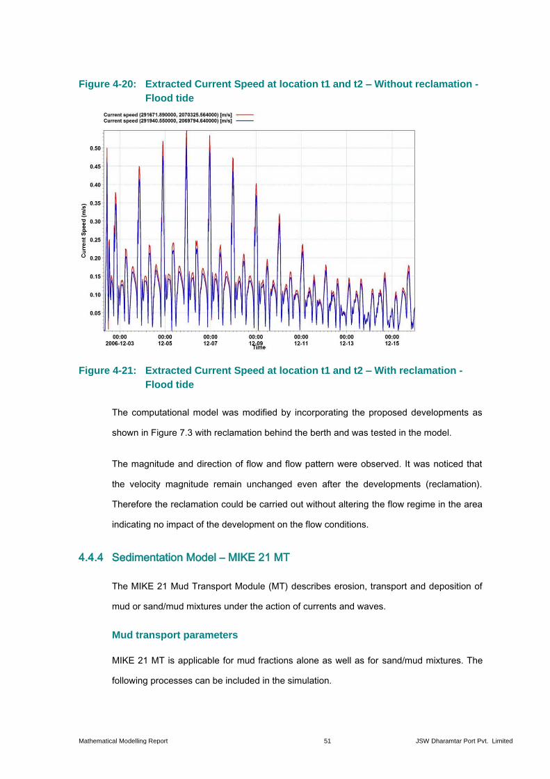
Mathematical Modelling Report 51 JSW Dharamtar Port Pvt. Limited
Figure 4-20: Extracted Current Speed at location t1 and t2 – Without reclamation -
Flood tide
Figure 4-21: Extracted Current Speed at location t1 and t2 – With reclamation -
Flood tide
The computational model was modified by incorporating the proposed developments as
shown in Figure 7.3 with reclamation behind the berth and was tested in the model.
The magnitude and direction of flow and flow pattern were observed. It was noticed that
the velocity magnitude remain unchanged even after the developments (reclamation).
Therefore the reclamation could be carried out without altering the flow regime in the area
indicating no impact of the development on the flow conditions.
4.4.4 Sedimentation Model – MIKE 21 MT
The MIKE 21 Mud Transport Module (MT) describes erosion, transport and deposition of
mud or sand/mud mixtures under the action of currents and waves.
Mud transport parameters
MIKE 21 MT is applicable for mud fractions alone as well as for sand/mud mixtures. The
following processes can be included in the simulation.

Mathematical Modelling Report 52 JSW Dharamtar Port Pvt. Limited
Forcing by waves
Sliding
Salt-flocculation
Detailed description of the settling process
Layered description of the bed, and
Morphological update of the bed
In the MT-module, the settling velocity varies, according to the salinity ( if included) and
the concentration taking into account flocculation in the water column. Furthermore,
hindered settling and consolidation in the fluid mud and under consolidated bed are
included in the model. Bed erosion can be either non-uniform, i.e. the erosion of soft and
partly consolidated bed, or uniform, i.e. the erosion of a dense and consolidated bed. The
bed is described as layered and characterized by the density and shear strength.
The Mud Transport Module can be applied to the study of engineering problems such as:
Sediment transport studies for fine cohesive materials or sand/mud mixtures in
estuaries and coastal areas in which environmental aspects are involved and
degradation of water quality may occur.
Siltation in harbour, navigational fairways, canals, rivers and reservoirs.
Dredging studies.
4.4.5 Model Set up – MIKE 21 MT
Bathymetry and the boundary conditions used in this setup are same applied in the local
model described in the chapter 4, section 5.5. Inlet and outfall points are introduced in the
bathymetry dredged up to 5 m. Local area extracted from modified bathymetry is shown in
Figure 4.13.
Model was executed for the period of 1day during non- monsoon as well as monsoon
conditions. Details on the set-up of MIKE 21 MT modules are provided in Table 4.3. Initial
and boundary concentration taken during non-monsoon and monsoon are provided in
table 4.4.
The model was then enforced for predicting the siltation pattern with the proposed using a
dredged depth of 3.5 m. The TSS concentration as indicated in chapter 3 was used. The
total annual siltation was found to be around 0.75 million cum per annum. It is observed

Mathematical Modelling Report 53 JSW Dharamtar Port Pvt. Limited
that the average depth of sediment deposition in the approach channel varies from 5 to 7
cm over a period of six months covering monsoon season. The estimated sedimentation in
the entire harbour region including approach channel and turning circle works out to be of
the order of 1-1.25 M Cu m which is based on the model study and literature survey of the
earlier studies.
Table 4-3: Parameters applied in the model simulations
S. No Parameters Value
1 No. of grain size fractions 1
2 No. of bed layer 1
3 Settling velocity 0. 05 m/s
4 Critical shear stress for deposition 0.05 N /m2
5 Power of erosion 1
6 Erosion coefficient 0.00001 kg/m2/s
7 Critical shear stress for erosion 0.05 N/m2
8 Density of bed layer 180 kg/m3
9 Bed roughness 0.001 m
Table 4-4: Concentration applied during non-monsoon and monsoon
period
S. No Parameters Value
1 Initial sediment concentration (non- monsoon) 0.004 kg /m3
3 Sediment concentration at downstream
boundary (non- monsoon) 0.0191 kg /m
3
4 Sediment concentration at upstream boundary
(non- monsoon) 0.0443 kg /m
3
5 Initial sediment concentration (monsoon) 0.02 kg /m3
6 Sediment concentration at downstream
boundary (monsoon) 0.02 kg /m
3
7 Sediment concentration at upstream boundary
(monsoon) 0.03 kg /m
3
Mathematical Modelling Report 54 JSW Dharamtar Port Pvt. Limited
5.4.5 Wave tranquillity
There is no wave effect near the proposed development as it is about 26 km from the sea
mouth. Waves cannot enter the creek due to restriction of width and depth.
5.4.6 Shoreline Evolution due to Construction
The model studies indicates no changes in the bank line of the river, as the eroding forces
due to the increase in the flow velocity due to the development is low.
This was also ascertained by studying the bank line evolution over the years.
4.5 Disposal of the Dredged sediments
The dredged sediments from the capital and the maintenance dredging would be disposed
at the established Mumbai Port Dumping ground on the high sea. This is an established
dumping ground and no additional study would be required for the same.

Mathematical Modelling Report 55 JSW Dharamtar Port Pvt. Limited
5 Conclusions and Recommendations
5.1 Conclusions
The study suggests that the proposed developments have negligible impact on the coastal
morphology of the creek. The following broad conclusions can be drawn
Dredging up to 5m of depth is proposed for the approach channel and the jetty
location. This would increase the flow channelization and flow efficiency of the river
(creek).
About 1 to 1.25 million m3 of maintenance dredging is required for a 5 m depth
channel.
There is no wave impact inside the port.
The coastal geo-morphology is not affected by the reclamation of 50 m width, as the
width is small in comparison to the river width.
The disposal of the dredged sediments can be done at the existing Mumbai Port
grounds.
5.2 Recommendations
The proposed development would have no or negligible impact on the river morphology
and the flow hydrodynamics, hence the development is recommended.