Lecture 6InterpolationDirect Method & Lagrange Method

For Slides Thanks toDr. S. M. Lutful KabirVisiting Professor, BRAC University& Professor, BUET

Numerical Methods

2

What is interpolation?

Many times, data is given only at discrete points such as

........... . So, how then does one find the value of y at any other value of x ?

Well, a continuous function f(x) may be used to represent the n+1 data values with f(x) passing through the n+1 points (Figure 1).

Then one can find the value of y at any other value of x. This is called interpolation.

LxUx Lxf Uxfrx %a mxf ,, 00 yx

,, 00 yx ,, 11 yx ,, 22 yx nn yx , ,, 11 nn yx

(x1,y1

)

(x2,y2

)(x0,y0

)

(x3,y3

)

x

y

f(x)

Figure 1

3

Polynomial interpolation?

Of course, if new ‘x’ falls outside the range of x for which the data is given, it is no longer interpolation but instead is called extrapolation.

So what kind of function f(x) should one choose? A polynomial is a common choice for an interpolating function because polynomials are easy to evaluate, differentiate, and integraterelative to other choices such as a trigonometric and exponential series

Polynomial interpolation involves finding a polynomial of order n that passes through the n+1 points

4

Direct Method of Interpolation

One of the methods of interpolation is called the direct method.

Other methods include the Lagrangian interpolation method and Newton’s divided difference polynomial method

The direct method of interpolation is based on the following premise. Given n+1 data points, fit a polynomial of order n as given below

(1) through the data, where a0, a1, a2,....... an+1, an are

real constants.

nn xaxaay ...............10

5

Direct Method of Interpolation (continued)

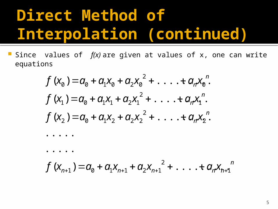
Since values of f(x) are given at values of x, one can write equations

nnnnnn

nn

nn

nn

xaxaxaaxf

xaxaxaaxf

xaxaxaaxf

xaxaxaaxf

12

121101

22

222102

12

121101

02

020100

.........)(

.....

.....

.........)(

.........)(

.........)(

6

Direct Method of Interpolation (continued)

Then the constants, can be found by solving the simultaneous linear equations.

To find the value of f(x) at a given value of x, simply substitute the value of x in Equation 1.

But, it is not necessary to use all the data points.

How does one then choose the order of the polynomial and what data points to use?

This concept and the direct method of interpolation are best illustrated using examples

7

Example 1

The upward velocity of a rocket is given as a function of time in Table 1. Corresponding graph is shown in Figure 1

Time (s) Velocity (m/s)0 0

10 227.04

15 362.78

20 517.35

22.5 602.97

30 901.67

t )(tv

Table 1: Velocity as function of time Figure 1: Graph of Velocity

Determine the value of the velocity at t = 16seconds using the direct method of interpolation and a first order polynomial.

8

Solution to example 1

For first order polynomial interpolation (also called linear interpolation), the velocity is given by

00 , yx

11, yx

xf1

xy

Figure 3 Linear interpolation

y

x(x0 , y0)

(x1 , y1)

f1(x)

9

Solution to example 1 (continued)

Since we want to find the velocity at t=16 sec, and we are using a first order polynomial, we need to choose the two data points that are closest to t = 16 sec that also bracket t=16 sec to evaluate it. The two points are t0=15 sec and t1=20 sec

Then t0=15, v(t0)=362.78 a0=-100.93t1=20, v(t1)=517.35 a1=30.914

Givesv(15)=a0+a1 x 15=362.78 v(t)=ao+a1tv(20)=a0+a1 x 20=517.35 v(16)=393.7

10

Example 2 Determine the value of the velocity at t = 16 seconds using the

direct method of interpolation and a second order polynomial.

00 , yx

11, yx

22 , yx

xf2

SolutionFor second order polynomial interpolation (also called quadratic interpolation), the velocity is given by

v(t)=a0+a1t+a2t2

y

x

x0 , y0

x1 , y1

x2 , y2

f(x)

11

Solution to example 2 (continued)

 Since we want to find the velocity at t=16, and we are using a second order polynomial, we need to choose the three data points that are closest to t = 16 that also bracket t = 16 to evaluate it. The three points are t0=10, t1=15 and t2=20

Then v(10)=227.04=a0+a1 x 10+a2 x 102

v(15)=362.78=a0+a1 x 15+a2 x 152 v(20)=517.35=a0+a1 x 20+a2 x 202

They gives, a0=12.05a1=17.733a2=0.3766

12

Solution to example 2 (continued)

Hence v(t)=12.05+17.733t+0.3766t2

V(16)=392.19 m/s

The absolute relative approximate error obtained between the results from the first and second order polynomial is

a

10019.392

70.39319.392

a

%38410.0

13

Example 3

For the rocket problem of the previous examples

a) Determine the value of the velocity at t=16 seconds using the direct method of interpolation and a third order polynomial.

b) Find the absolute relative approximate error for the third order polynomial approximation.

c) Using the third order polynomial interpolant for velocity from part (a), find the distance covered by the rocket from t=11 s to t=16 s.

d) Using the third order polynomial interpolant for velocity from part (a), find the acceleration of the rocket at t=16s.

14

Solution to example 3

For third order polynomial interpolation (also called cubic interpolation), we choose the velocity given by 3

32

210 tatataatv

(x0 , y0)

(x1 , y1)

(x2 , y2)

(x3 , y3)

x

y

f3(x)

15

Solution to example 3 (continued)

Since we want to find the velocity at t=16, and we are using a third order polynomial, we need to choose the four data points closest to and also bracket that.

The four points are (t0, v0)=(10, 227.04), (t1, v1)=(15, 362.78), (t2, v2)=(20, 517.35) and (t3, v3)=(22.5, 602.97)

Solving the above four equations gives a0= - 4.2540 a1= 21.266

a2= 0.13204a3= 0.0054347

Hence, v(t) = - 4.2540 + 21.266 t + 0.13204 t2 + 0.0054347 t3

So, v(16)= 392.06 m/s

16

Solution to example 3 (continued)

b) The absolute percentage relative approximate error for the value obtained for v(16) between second and third order polynomial is

c) The distance covered by the rocket between

t=11s and t=16s can be calculated from the interpolating polynomial

Note that the polynomial is valid between t = 10 s and t = 22.5 s and hence includes the limits of integration of t = 11 s and t = 16 s

a

10006.392

19.39206.392

a %033269.0

5.2210,0054347.013204.0266.212540.4 32 tttttv

17

Solution to example 3 (continued)

16

11

1116 dttvss

dtttt 16

11

32 )0054347.013204.0266.212540.4(

16

11

432

40054347.0

313204.0

2266.212540.4

tttt=

= 1605m

d) The acceleration at t=16sec is given by,

16

16

t

tvdt

da

5.2210,0054347.013204.0266.212540.4 32 tttttv

32 0054347.013204.0266.212540.4)( tttdt

dta

So, a(16) = 29.665 m/s2

18

Solving the coefficients of polynomial having high order

n

n

n

nn

nn

nnnnn

nn

nn

nnnnn

nn

nn

nnnnn

nnn

nnn

nnn

n

n

n

a

a

a

a

a

a

xxxxxx

xxxxxx

xxxxxx

xxxxxx

xxxxxx

xxxxxx

xf

xf

xf

xf

xf

xf

1

2

3

1

0

1232

111

21

31

211

212

22

32

222

21

22

232

222

11

12

131

211

01

02

030

200

1

2

2

1

0

....

....

.............1

..........1

..........1

......

......

.............1

.............1

............1

)(

)(

)(

.....

.....

)(

)(

)(

[Y] = [C] [A] Since [Y] = [C] [A] So, [A] = [C]-1 [Y]

If the polynomial is of nth order, there are n numbers of unknowns, how to find out them?

One way is to arrange the equations in matrix form as shown below:

19

Langrange Method

The Lagrangian interpolating polynomial is given by

where n in fn(x) stands for the nth order polynomial that approximates the function y=f(x) given at n+1 data points as (x0,y0), (x1,y1), (x2,y2),……. (xn-1,yn-1), (xn, yn) and

Li(x) is a weighting function that includes a product of n-1 terms with terms of j = i omitted. The application of Lagrangian interpolation will be clarified using an example.

n

iiin xfxLxf

0

)()()(

n

ijj ji

ji xx

xxxL

0

)(

20

Example 4

Determine the value of the velocity of the rocket problem at t=16 seconds using a first order Lagrange polynomial.

Solution For first order polynomial interpolation (also

called linear interpolation), the velocity is given by

1

0

)()()(i

ii tvtLtv

)()()()( 1100 tvtLtvtL

1

00 0

0 )(

jj j

j

tt

tttL

10

1

tt

tt

1

10 1

1 )(

jj j

j

tt

tttL

01

0

tt

tt

Hence,

v(16) = 393.69 m/s

)()()( 101

00

10

1 tvtt

tttv

tt

tttv

21

Solution to example 4

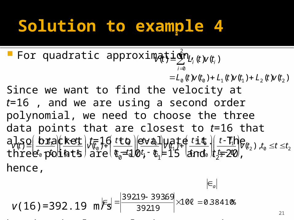
For quadratic approximation,

2

0

)()()(i

ii tvtLtv

)()()()()()( 221100 tvtLtvtLtvtL

16t16t16t

20 and ,15 ,10 210 ttt

Since we want to find the velocity at

to evaluate it. The three points are

.

Since we want to find the velocity at t=16 , and we are using a second order polynomial, we need to choose the three data points that are closest to t=16 that also bracket t=16 to evaluate it. The three points are t0=10, t1=15 and t2=20, hence,

v(16)=392.19 m/s

b) The absolute relative approximate error with respect to direct method is

20212

1

02

01

21

2

01

00

20

2

10

1 ),()()()( ttttvtt

tt

tt

tttv

tt

tt

tt

tttv

tt

tt

tt

tttv

a

10019.392

69.39319.392

a %38410.0

22

Flow Chart for Direct Method

n

x(i), y(i), i=1,1,....n+1

xu

for i=1..n+1

xu, fxu

Start

FT

for j=1..n+1

TF

c(i,j)=x(i)^(j-1)

ci=inv(c)

for i=1..n+1 F

T

for j=1..n+1T

a(i)=0

a(i)=a(i)+ci(i,j)*y(j)

for i=1..n+1T

fxu=0

fxu=fxu+a(i)*xu^(i-1)

F

F

1

2

3

4

5

6

7

8

16

9

10

11

12

13

14

15End

17

Flow Chart for Langrage method

23

n L(i)=1

L(i)=L(i)*(xu-x(j))/(x(i)-x(j))

fxu=fxu+L(i)*y(i)

x(i), y(i), i=1...n+1

xu

for j=1..n+1 j : i

fxu=0

for i=1..n+1

xu, fxu

Start

==

TF

T

F

5

1

2

3

4

6

10

8

7

9

11

10

End12

24

Thanks