Numerical Methods in MATLAB

Center for Interdisciplinary Research and Consulting

Department of Mathematics and Statistics

University of Maryland, Baltimore County

www.umbc.edu/circ

Winter 2012

Mission and Goals: The Center for Interdisciplinary Research and Consulting(CIRC) is a consulting service on mathematics and statistics provided by the Depart-ment of Mathematics and Statistics at UMBC. Established in 2003, CIRC is dedicatedto support interdisciplinary research for the UMBC campus community and the pub-lic at large. We provide a full range of consulting services from free initial consultingto long term support for research programs.

CIRC offers mathematical and statistical expertise in broad areas of applications,including biological sciences, engineering, and the social sciences. On the mathematicsside, particular strengths include techniques of parallel computing and assistance withsoftware packages such as MATLAB and COMSOL Multiphysics (formerly known asFEMLAB). On the statistics side, areas of particular strength include Toxicology,Industrial Hygiene, Bioequivalence, Biomechanical Engineering, Environmental Sci-ence, Finance, Information Theory, and packages such as SAS, SPSS, and S-Plus.

Copyright c© 2003–2012 by the Center for Interdisciplinary Research and Consult-ing, Department of Mathematics and Statistics, University of Maryland, BaltimoreCounty. All Rights Reserved.

This tutorial is provided as a service of CIRC to the community for personal usesonly. Any use beyond this is only acceptable with prior permission from CIRC.

This document is under constant development and will periodically be updated. Stan-dard disclaimers apply.

Acknowledgements: We gratefully acknowledge the efforts of the CIRC researchassistants and students in Math/Stat 750 Introduction to Interdisciplinary Consultingin developing this tutorial series.

MATLAB is a registered trademark of The MathWorks, Inc., www.mathworks.com.

3

1 Introduction

In this tutorial, we will introduce some of the numerical methods available in Matlab.Our goal is to provide some snap-shots of the wide variety of computational tools thatMatlab provides. We will look at some optimization routines, where we mainly focuson unconstrained optimization. Next, we discuss curve fitting and approximation offunctions using Matlab. Our final topic will be numerical ODEs in Matlab.

Matlab provides a number of specialized toolboxes, which extend the capabilitiesof the software. We will have a brief overview of the various toolboxes in Matlab andwill provide a list of some available toolboxes.

• Numerical Optimization

• Data Fitting / Approximation

• Numerical ODEs

• Matlab Toolboxes

2 Unconstrained Optimization

The commands we discuss in this section are two of the several optimization routinesavailable in Matlab. First we discuss fminbnd, which is used to minimize functionsof one variable. The command,

[x fval] = fminbnd(f, a, b)

finds a local minimizer of the function f in the interval [a, b]. Here x is the localminimizer found by the command and fval is the value of the function f at that point.For complete discussion of fminbnd readers can refer to the Matlab’s documentations.Here we illustrate the use of fminbnd in an example.

Consider the function f(x) = cos(x)− 2 ln(x) on the interval, [π2, 4π]. The plot of

the function is depicted in Figure 1. We can first define the function f(x) in Matlabusing

f = @(x)(cos(x) - 2*log(x))

Then we proceed by the following,

>> [x fval] = fminbnd(f, 2, 4)

x =

3.7108

4 2 UNCONSTRAINED OPTIMIZATION

Figure 1: Plot of f(x) = cos(x)− 2 ln(x).

fval =

-3.4648

We see that fminbnd returns the (approximate) minimizer of f(x) in the interval [2, 4]and also computes the value of f(x) at the minimizer. The readers can try to find the(global) minimizer of f(x) which is seen to be somewhere in [8, 10] using fminbnd.

The next (unconstrained) optimization command we discuss is fminsearch whichcan be used to find a local minimizer of a function of several variables. The command,

[x fval] = fminsearch(f,x0)

finds a local minimizer of the function f given the initial guess x0. For completediscussion of fminsearch readers can refer to the Matlab’s documentations. Here weillustrate the use of fminsearch in an example.

For a simple example, we minimize the function f(x, y) = x2 + y2 which clearlyhas its minimizer at (0, 0). Let’s choose an initial guess of x0 = (0, 0). The followingMatlab commands illustrate the usage of fminsearch

>> f = @(x)(x(1)^2+x(2)^2);

>> x0 = [1;1];

>> [x fval] = fminsearch(f, x0)

x =

1.0e-04 *

-0.2102

5

0.2548

fval =

1.0915e-09

Of course, reader can try fminsearch on more complicated problems and see theresults.

For more information on optimization routines in Matlab, reader can investigateMatlab’s Optimization Toolbox which includes several powerful optimization toolswhich can be used to solve both unconstrained and constrained linear and non-linearoptimization problems.

3 Curve-Fitting

Here we consider the problem of fitting a polynomial of degree (at most) k into thedata points (xi, yi); to do this, we use the command,

p = polyfit(x, y, k)

which fits a polynomial of degree k into the given data points. The output argumentp is a vector which contains the coefficients of the interpolating polynomial. Themethod used is least squares, in which we choose a polynomial P of degree k whichminimizes the following:

m∑i=1

[P (xi)− yi]2. (3.1)

For example, say we are given the data points

xi yi

--------

1 1

2 0.5

3 1

4 2.5

5 3

6 4

7 5

Suppose we would like to fit a polynomial of degree three into the given data points.We can use the following Matlab commands to get the interpolating polynomial.

>> xi = 1 : 7;

>> yi = [1 0.5 1 2.5 3 4 5];

>> p = polyfit(xi,yi,3);

6 3 CURVE-FITTING

Once we have the vector p which contains the coefficients of the interpolating poly-nomial we can use the Matlab function polyval to evaluate the approximating poly-nomial over a given range of x values. We can proceed as follows:

>> x = 1 :0.1: 7;

>> y = polyval(p, x);

>> plot(xi, yi, ’*’, x, y)

Which produces the Figure 2.

Figure 2: Data fitting in Matlab

Another useful idea is using polyfit to find an approximating polynomial for agiven function. The idea is useful because polynomials are much simpler to work with.For example one can easily integrate or differential polynomials while it may not beso easy to do the same for a function which is not so well behaved. As an example, weconsider the problem of approximating the function sin(

√(x)) on the interval [0, 2π].

The following Matlab commands show how one selects a numerical grid to get datapoints which can be used to approximate the function using a polynomial of degreek (in a least-squares sense).

>> f = @(x)(sin(sqrt(x)));

>> xi = [0 : 0.1 : 2*pi];

>> yi = f(xi);

>> p = polyfit(xi,yi,4);

To see how the function and its approximation compare, we can use the followingcommands,

>> x = [0 : 0.01 : 2*pi];

>> y = polyval(p, x);

>> plot(x, f(x), x, y, ’--’);

The result can be seen in Figure 3.

7

Figure 3: Approximation of a function using polynomial data fitting

4 Numerical ODEs

In this section we discuss numerical ordinary differential equations in Matlab. Matlabprovides a number of ODE solvers; we will focus our attention to ode45 which usesa four stage Runge-kutta method to solve a give ordinary differential equation. Wewill first see how ones an initial value problem of form

dy

dt= f(t, y),

y(t0) = y0.

We can solve such problems using

[T Y]=ode45(f, tspan, y0)

In the above syntax, the input argument f specifies the right hand side function ofthe differential equations, tspan is the time interval in which we want to solve theequation, and y0 is the initial value. The output argument Y gives the numericalsolution over the discretized time interval T. Consider the following problem,

dy

dt= t− y,

y(0) = 1.

One can solve this problem analytically to get the solution, y(t) = 2e−t + t − 1. Tosolve the problem numerically, we can use

>> f = @(t, y)(t - y)

f =

@(t, y)(t - y)

>> y0=1;

>> [T Y] = ode45(f, [0 2], y0);

8 4 NUMERICAL ODES

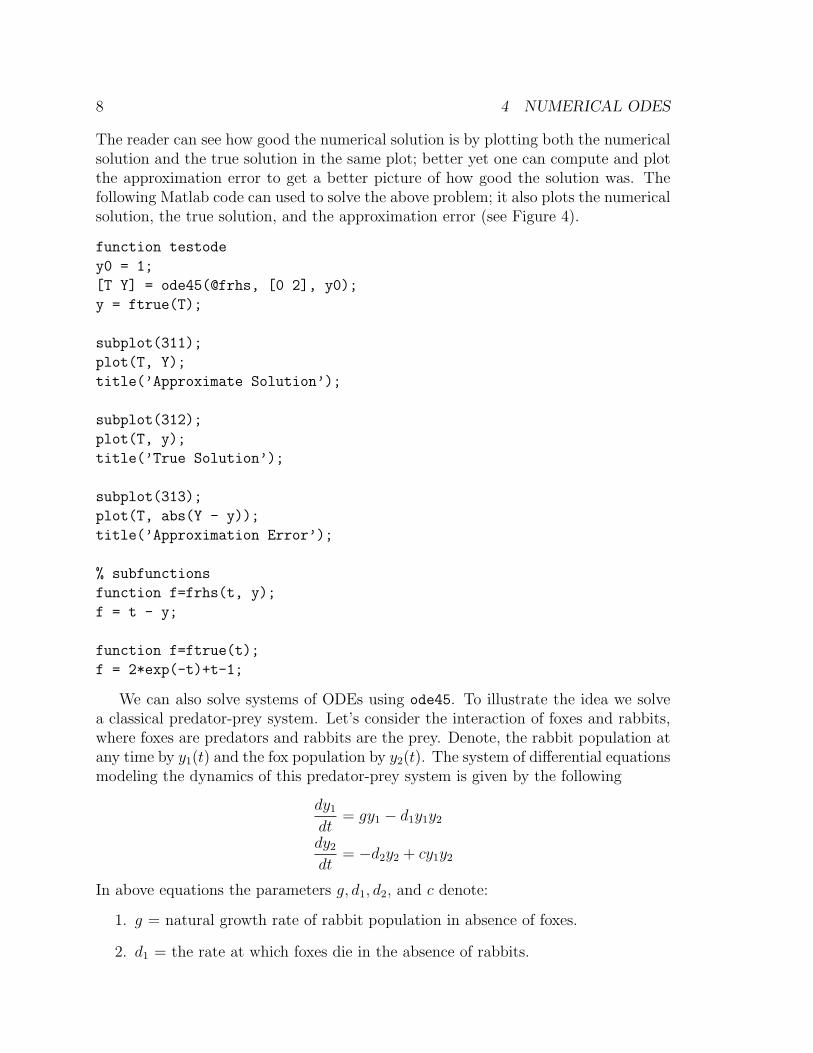
The reader can see how good the numerical solution is by plotting both the numericalsolution and the true solution in the same plot; better yet one can compute and plotthe approximation error to get a better picture of how good the solution was. Thefollowing Matlab code can used to solve the above problem; it also plots the numericalsolution, the true solution, and the approximation error (see Figure 4).

function testode

y0 = 1;

[T Y] = ode45(@frhs, [0 2], y0);

y = ftrue(T);

subplot(311);

plot(T, Y);

title(’Approximate Solution’);

subplot(312);

plot(T, y);

title(’True Solution’);

subplot(313);

plot(T, abs(Y - y));

title(’Approximation Error’);

% subfunctions

function f=frhs(t, y);

f = t - y;

function f=ftrue(t);

f = 2*exp(-t)+t-1;

We can also solve systems of ODEs using ode45. To illustrate the idea we solvea classical predator-prey system. Let’s consider the interaction of foxes and rabbits,where foxes are predators and rabbits are the prey. Denote, the rabbit population atany time by y1(t) and the fox population by y2(t). The system of differential equationsmodeling the dynamics of this predator-prey system is given by the following

dy1

dt= gy1 − d1y1y2

dy2

dt= −d2y2 + cy1y2

In above equations the parameters g, d1, d2, and c denote:

1. g = natural growth rate of rabbit population in absence of foxes.

2. d1 = the rate at which foxes die in the absence of rabbits.

9

Figure 4: Using ode45 to solve an ODE

3. d2 = the death rate per each (deadly) encounter of rabbits due to foxes.

4. c = the contribution to fox population of each (food making) encounter ofrabbits and foxes to fox population.

In addition to specifying the model parameters, we also need to specify the initialpopulation of foxes and rabbits at t = 0. Let’s choose the model parameters as below:

• g = 0.04;

• d1 = 0.001;

• d2 = 0.1;

• c = 0.002;

Also, we assume the initial populations start at y1(0) = 100 and y2(0) = 100. Tosolve the resulting initial value problem, we can use ode45; the Matlab functionpredatorprey provided below solves the problem using ode45 and plots the popula-tions of foxes and rabbits on the same plot (Figure 5); moreover, the function createsa phase-plane diagram (Figure 5) which is a useful tool in analyzing such systems.

10 4 NUMERICAL ODES

function predatorprey

[T,Y] = ode45(@yprime,[0 100],[100 100]);

subplot(2,1,1);

plot(T,Y(:,1),’-’, T,Y(:,2), ’--’);

title(’Population Dynamics of Foxes and Rabbits’);

legend(’Rabbit Population’, ’Fox Population’);

xlabel(’t’);

ylabel(’Population’);

grid on;

subplot(2,1,2);

plot(Y(:,1), Y(:,2));

title(’Phase Plane Diagram for the fox-rabbit population’);

xlabel(’Rabbits’);

ylabel(’Foxes’);

grid on;

%rhs function

function dy = yprime(t, y)

g = 0.4;

d1 = 0.001;

d2 = 0.1;

c = 0.002;

dy = [g*y(1)-d1*y(1)*y(2);

c*y(1)*y(2) - d2*y(2)];

11

Figure 5: Dynamics of a predator prey (fox/rabbit) system

The reader can further experiment with the above Matlab code to see the outcomewith different parameters and different initial populations.

12 4 NUMERICAL ODES

Our discussion of Matlab’s ODE solvers here focused on the example of the func-tion ode45, which is Matlab’s most popular ODE solver. Matlab has a suite of solvers,see doc ode45 for full documentation and recommendations for when to use whichmethod in table form. We complement this table here by discussing the methods andproviding some additional information. See this documentation also for the list ofoptions used to control the method, such as relative and absolute tolerances on theerror estimator, as well as for a list of references on the subject of ODE solvers andthe methods in particular.

All ODE solvers in Matlab use the same function interface, so it is easy to tryseveral methods on the same problem and observe their behavior. Also, all methodscompute an estimator for the error of the solution that is used to automatically selectthe size of the time step and also of the method order, if it is variable. ODE problemsare roughly classified into stiff and nonstiff problems. General-purpose ODE solversin Matlab that are appropriate for stiff problems are indicated by the letter “s” atthe end of their names, namely ode15s and ode23s. The most important nonstiffsolvers are 45 and ode113. The numbers in the names of the two methods ode15s andode113 that are variable-order methods indicate the method order ranging from 1 to5 and from 1 to 13, respectively. All other methods are fixed-order methods with thefirst number indicating the order of the method, such as 4 in ode45 and 2 in ode23s;the second number indicates the order of the second method used simultaneously inthe error estimator.

The technical definition of the term stiff is difficult, but their practical definitionis readily stated: A problem is stiff, if the automatic step size control of the methodchooses small steps even for large tolerances. This means that the step sizes arelimited by the stability of the method and not the accuracy requested by the user.Note that all ODE solvers in Matlab use automatic step size control based on asophisticated error estimator, hence the accuracy of their solution is ensured; but ifit takes a longer time to compute the solution with nonstiff solvers such as ode45 orode113 than with a stiff solver such as ode15s, the problem is considered stiff. Insummary, for a particular problem, try ode45 or ode113 as potential nonstiff solversand try also ode15s as potential stiff solvers. Then continue using whichever methodperformed most efficiently.

13

5 Matlab Toolboxes

In this section, we will discuss Matlab Toolboxes. In general, Matlab toolboxes extendthe capabilities of Matlab by providing highly efficient routines which are specializedto handle specific situations. For example, if one is solving some problems in the areaof neural networks, the Neural Network Toolbox provides powerful tools to handleproblems of that type. As another example, Matlab’s Statistics Toolbox provides awide range of statistical routines.

A good way to learn about a Matlab Toolbox is studying the associated Get-ting Started Guide; another good place to start is the user’s guide for the associatedToolbox. For example, in Figure 6, we have displayed the help screen for Matlab’sStatistics Toolbox (from Matlab’s Help facility). We can see the various documenta-tions provided for a toolbox.

Figure 6: Matlab’s Statistics Toolbox

To give the readers an idea of the available Matlab toolboxes, a list of widely usedMatlab Toolboxes is provided in Table 1.

To find out which Toolboxes are available in your version of Matlab you can type

ver

in Matlab’s command prompt. Issuing the ver command will provide something likethe following:

14 5 MATLAB TOOLBOXES

Math and OptimizationOptimization ToolboxSymbolic Math ToolboxExtended Symbolic Math ToolboxPartial Differential Equation ToolboxGenetic Algorithm and Direct Search Toolbox

Statistics and Data AnalysisStatistics ToolboxNeural Network ToolboxCurve Fitting ToolboxSpline ToolboxModel-Based Calibration ToolboxControl System Design and AnalysisControl System ToolboxSystem Identification ToolboxFuzzy Logic ToolboxRobust Control ToolboxModel Predictive Control ToolboxAerospace Toolbox

Signal Processing and CommunicationsSignal Processing ToolboxCommunications ToolboxFilter Design ToolboxFilter Design HDL Coder Wavelet ToolboxFixed-Point Toolbox RF Toolbox

Image ProcessingImage Processing ToolboxImage Acquisition ToolboxMapping Toolbox

Test and MeasurementData Acquisition ToolboxInstrument Control ToolboxImage Acquisition ToolboxSystemTest OPC Toolbox

Computational BiologyBioinformatics Toolbox

Financial Modeling and AnalysisFinancial ToolboxFinancial Derivatives ToolboxGARCH ToolboxDatafeed ToolboxFixed-Income Toolbox

Table 1: A list of Matlab Toolboxes

15

>> ver

--------------------------------------------------------------------------------

MATLAB Version 7.7.0.471 (R2008b)

MATLAB License Number: 334413

Operating System: Linux 2.6.18-92.1.18.el5 #1 SMP Wed Nov 5 09:00:13 EST 2008

i686

Java VM Version: Java 1.6.0_04 with Sun Microsystems Inc. Java HotSpot(TM)

Client VM mixed mode

--------------------------------------------------------------------------------

MATLAB Version 7.7 (R2008b)

Simulink Version 7.2 (R2008b)

Bioinformatics Toolbox Version 3.2 (R2008b)

Communications Blockset Version 4.1 (R2008b)

Communications Toolbox Version 4.2 (R2008b)

Control System Toolbox Version 8.2 (R2008b)

Curve Fitting Toolbox Version 1.2.2 (R2008b)

Fuzzy Logic Toolbox Version 2.2.8 (R2008b)

Image Processing Toolbox Version 6.2 (R2008b)

Instrument Control Toolbox Version 2.7 (R2008b)

MATLAB Compiler Version 4.9 (R2008b)

Mapping Toolbox Version 2.7.1 (R2008b)

Neural Network Toolbox Version 6.0.1 (R2008b)

Optimization Toolbox Version 4.1 (R2008b)

Partial Differential Equation Toolbox Version 1.0.13 (R2008b)

Signal Processing Blockset Version 6.8 (R2008b)

Signal Processing Toolbox Version 6.10 (R2008b)

SimMechanics Version 3.0 (R2008b)

Simscape Version 3.0 (R2008b)

Spline Toolbox Version 3.3.5 (R2008b)

Stateflow Version 7.2 (R2008b)

Statistics Toolbox Version 7.0 (R2008b)

Symbolic Math Toolbox Version 5.1 (R2008b)

System Identification Toolbox Version 7.2.1 (R2008b)

Wavelet Toolbox Version 4.3 (R2008b)

Of course, the results may vary depending on the system on which the commandver is issued.