Numerical Methods and Advanced Simulation in …pontrell/pub/CERROLAZA_chapter20.pdfNumerical Methods and Advanced Simulation in Biomechanics and Biological Processes Edited by Miguel

Numerical Methods andAdvanced Simulation inBiomechanics and BiologicalProcesses

Edited by

Miguel Cerrolaza, Sandra J. Shefelbineand Diego Garzon-Alvarado

Academic Press is an imprint of Elsevier125 London Wall, London EC2Y 5AS, United Kingdom525 B Street, Suite 1800, San Diego, CA 92101-4495, United States50 Hampshire Street, 5th Floor, Cambridge, MA 02139, United StatesThe Boulevard, Langford Lane, Kidlington, Oxford OX5 1GB, United Kingdom

Copyright © 2018 Elsevier Ltd. All rights reserved.

No part of this publication may be reproduced or transmitted in any form or by any means, electronic or mechanical, includingphotocopying, recording, or any information storage and retrieval system, without permission in writing from the publisher.Details on how to seek permission, further information about the Publisher’s permissions policies and our arrangementswith organizations such as the Copyright Clearance Center and the Copyright Licensing Agency, can be found at our website:www.elsevier.com/permissions.

This book and the individual contributions contained in it are protected under copyright by the Publisher (other than as may benoted herein).

NoticesKnowledge and best practice in this field are constantly changing. As new research and experience broaden our understanding,changes in research methods, professional practices, or medical treatment may become necessary.

Practitioners and researchers must always rely on their own experience and knowledge in evaluating and using any information,methods, compounds, or experiments described herein. In using such information or methods they should be mindful of theirown safety and the safety of others, including parties for whom they have a professional responsibility.

To the fullest extent of the law, neither the Publisher nor the authors, contributors, or editors, assume any liability for any injuryand/or damage to persons or property as a matter of products liability, negligence or otherwise, or from any use or operation ofany methods, products, instructions, or ideas contained in the material herein.

Library of Congress Cataloging-in-Publication DataA catalog record for this book is available from the Library of Congress

British Library Cataloguing-in-Publication DataA catalogue record for this book is available from the British Library

ISBN: 978-0-12-811718-7

For information on all Academic Press publications visitour website at https://www.elsevier.com/books-and-journals

Publisher: Mara E. ConnerAcquisition Editor: Fiona GeraghtyEditorial Project Manager: Jennifer PierceProduction Project Manager: Mohanapriyan RajendranDesigner: Victoria Pearson

Typeset by TNQ Books and Journals

Chapter 20

Multicomponent Lattice BoltzmannModels for Biological ApplicationsA. Montessori1, I. Halliday2, M. Lauricella3, S.V. Lishchuk2, G. Pontrelli3, T.J. Spencer2 and S. Succi3,4

1University of Rome “Roma Tre”, Rome, Italy; 2Sheffield Hallam University, United Kingdom; 3Istituto per le Applicazioni del Calcolo - CNR,

Roma, Italy; 4Harvard University, Cambridge, MA, United States

20.1 INTRODUCTION

In the last decade lattice Boltzmann (LB) methods have met with a huge success within the computational physicscommunity because of their capability to simulate a very wide range of fluid dynamics phenomena and beyond. The LBmodels for fluid dynamics were first developed to cure some shortcomings of the lattice gas automata, such as the spuriousinvariants and the statistical noise, while preserving the local nature of the collisional and the linearity of the streamingoperator along propagation characteristics. Since then, a great deal of effort has been devoted to the development of LBmodels capable of simulating complex flows across a wide range of scales of motion (Succi, 2015). In particular, LBmodels for nonideal fluids have seen a major boost in connection with the simulation of complex states of flowing matter,such as multiphase and multicomponent flows. The three basic LB multiphase methods are the color-fluid model (developedby Gunstensen et al., 1991.), the interparticle-potential model of Shan and Chen (1993), and the free-energy model(Swift et al., 1995). Here, we briefly outline the recent developments of each approach. The color-fluid model, proposed byRothman and Keller (1988) and further developed by Grunau et al. (1993), is based on a two-component LB model, fa,i(x, t)and fb,i(x, t), representing two different interacting fluids. The surface tension is encoded via a perturbation step namely, amodification of the original LB collision operator, while phase separation is maintained through a segregation step by forcingparticles to regions of the same color. In the pseudopotential model (Shan and Chen, 1993) the interactions between fluidcomponents are modeled through a modification of the collision operator by using an equilibrium velocity that includesan interactive force, which mimics an effective particleeparticle potential at a mesoscopic level. This force guaranteesphase separation and introduces surface tension effects. This model has been applied recently with considerable success(Montessori et al., 2015, Falcucci et al., 2013, Dollet et al., 2015). Moreover, it has been extended to include different van derWaals (vdW)elike equations of state by properly defining a suitable generalized functional form of the pseudopotential(Yuan and Schaefer, 2006, Qin, 2006). A multirange interaction model has been proposed to control the surface tensionindependently of the equation of state (Sbragaglia et al., 2007). The same can be done by modifying the attractive andrepulsive terms of a vdW-like equation of state (Montessori et al., 2015). The free-energy model employs a free-energyfunction to include surface tension effects in a thermodynamically consistent manner (Orlandini et al., 1995). In additionto the methods outlined above, other promising methods based on a combination of the LB equation with explicit interface-tracking schemes are under development. One approach uses Peskin’s (2002) distribution function for the interface force usedin the immersed boundary (IB) method (Lallemand et al., 2007). More recently, interface tracking using the volume of fluidapproach has been reported with promising results (Körner et al., 2005). In the following the pseudopotential approach formultiphase and multicomponent flows and the modified color-gradient method will be described in full detail, with a specialemphasis on their prospective biological applications.

Numerical Methods and Advanced Simulation in Biomechanics and Biological Processes. https://doi.org/10.1016/B978-0-12-811718-7.00020-4Copyright © 2018 Elsevier Ltd. All rights reserved.

357

20.2 THE LATTICE BOLTZMANN EQUATION

The LB equation with forcing terms reads as follows:

fiðx þ ciDt; t þ DtÞ � fiðx; tÞ ¼ �uDt½ fi � f eqi ðr; u þ F=urÞ� (20.1)

where fi(x, t) h f(x, v ¼ ci, t) is the discrete distribution function providing the probability of finding a particle atlattice site x at time t with discrete velocity ci, being i the lattice direction (Qian et al., 1992; Succi, 2001) (Fig. 20.1).In Eq. (20.1), u is the relaxation parameter and F is a shift force.

Eq. (20.1) describes the evolution of the discrete single-particle distribution function in terms of streaming (left-handside) and collision, in the form of a relaxation toward a local equilibrium (first term at right-hand side). The local equilibriaare computed as second-order expansion in the local Mach number, Ma ¼ u/cs, u being the macroscopic flow velocity and

cs ¼ ffiffiffiffiffiffiffiffi1=3

pthe lattice speed of sound:

f eqi ðx; tÞ ¼ wir

1 þ u$ci

c2sþ ðu$ciÞ2

2c4s� u$u

2c2s

!(20.2)

where wi are weights of the discrete equilibrium distribution functions and

rðx; tÞ ¼Xi

fiðx; tÞ; uðx; tÞ ¼Pifiðx; tÞcirðx; tÞ (20.3)

the fluid density and the flow velocity, respectively. The second term at the right-hand side of Eq. (20.1) accountsfor the effect of external/internal forces acting on the fluid molecules, such as gravity or, as we are going to describe inthe following, a pseudomolecular interactive force that mimics an effective particleeparticle potential at a mesoscopic levelthat promotes phase separation and introduces surface tension effects in a simple and efficient way (Shan and Chen, 1993).

20.3 THE PSEUDOPOTENTIAL APPROACH FOR MULTIPHASE ANDMULTICOMPONENT FLOWS

In the ShaneChen (SC) pseudopotential scheme, the nonideal force in Eq. (20.1) takes the form (Shan and Chen, 1993):

Fðx; tÞ ¼ �Gjðrðx; tÞÞDtXi

licijðrðx þ ciDt; tÞÞ (20.4)

FIGURE 20.1 Sketch of the 9-speed two-dimensional (D2Q9) (A) and 19-speed three-dimensional lattices (D3Q19) (B).

358 PART j VI Lattice Boltzmann Methods

where G is the strength of nonideal interactions, li are the coefficients for the nth isotropic lattice, and the generalizeddensity j(r) contributes the excess pressure in the nonideal equation of state:

p ¼ rc2s þ G

2j2ðrÞ. (20.5)

In the SC model, one has

jðrÞ ¼ 1 � e�r (20.6)

which gives a critical pressure pc ¼ (ln2 � 1/2)/3w 0.063 and a critical coupling Gc ¼ �4. We recall that negative G’scode for attraction, the only interaction in the SC model. Note that in the ideal gas limit r / 0, the SC equation of statedelivers p ¼ rc2s , with a fixed sound speed c2s ¼ 1/3.

20.3.1 Discretization of the Nonideal Forcing Term on Higher-Order Lattices

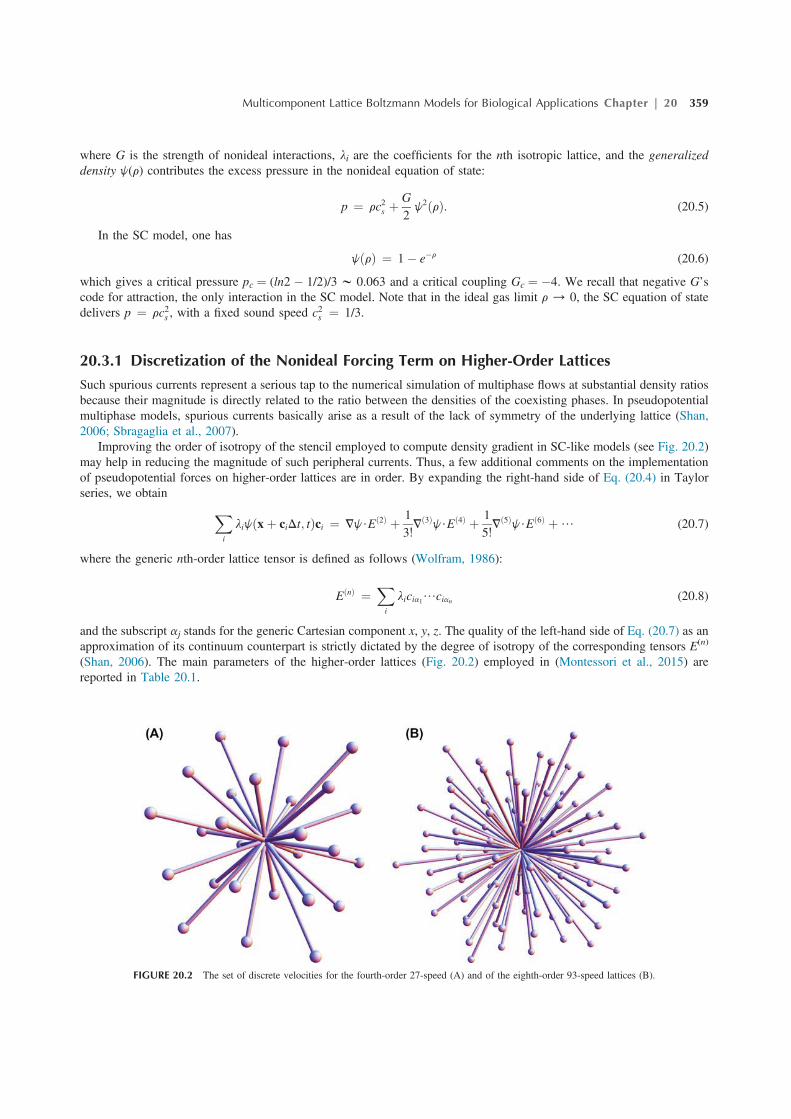
Such spurious currents represent a serious tap to the numerical simulation of multiphase flows at substantial density ratiosbecause their magnitude is directly related to the ratio between the densities of the coexisting phases. In pseudopotentialmultiphase models, spurious currents basically arise as a result of the lack of symmetry of the underlying lattice (Shan,2006; Sbragaglia et al., 2007).

Improving the order of isotropy of the stencil employed to compute density gradient in SC-like models (see Fig. 20.2)may help in reducing the magnitude of such peripheral currents. Thus, a few additional comments on the implementationof pseudopotential forces on higher-order lattices are in order. By expanding the right-hand side of Eq. (20.4) in Taylorseries, we obtain X

i

lijðx þ ciDt; tÞci ¼ Vj$Eð2Þ þ 13!Vð3Þj$Eð4Þ þ 1

5!Vð5Þj$Eð6Þ þ / (20.7)

where the generic nth-order lattice tensor is defined as follows (Wolfram, 1986):

EðnÞ ¼Xi

licia1/cian (20.8)

and the subscript aj stands for the generic Cartesian component x, y, z. The quality of the left-hand side of Eq. (20.7) as anapproximation of its continuum counterpart is strictly dictated by the degree of isotropy of the corresponding tensors E(n)

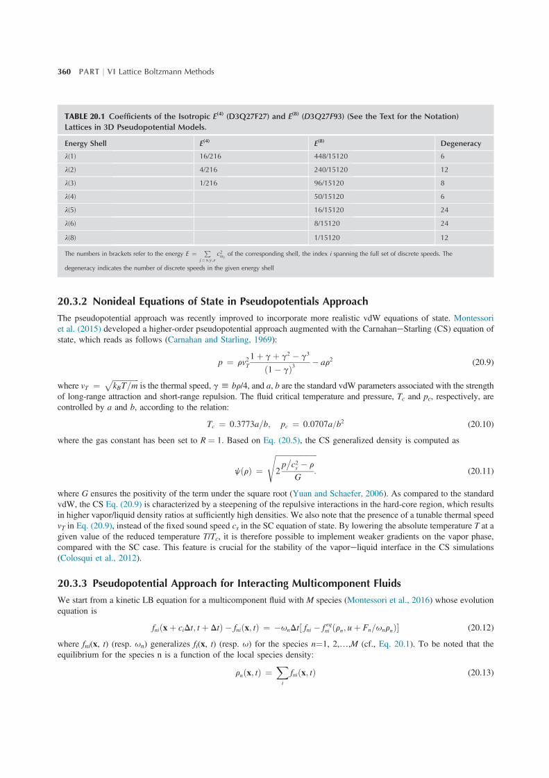
(Shan, 2006). The main parameters of the higher-order lattices (Fig. 20.2) employed in (Montessori et al., 2015) arereported in Table 20.1.

FIGURE 20.2 The set of discrete velocities for the fourth-order 27-speed (A) and of the eighth-order 93-speed lattices (B).

Multicomponent Lattice Boltzmann Models for Biological Applications Chapter | 20 359

20.3.2 Nonideal Equations of State in Pseudopotentials Approach

The pseudopotential approach was recently improved to incorporate more realistic vdW equations of state. Montessoriet al. (2015) developed a higher-order pseudopotential approach augmented with the CarnahaneStarling (CS) equation ofstate, which reads as follows (Carnahan and Starling, 1969):

p ¼ rv2T1 þ g þ g2 � g3

ð1 � gÞ3 � ar2 (20.9)

where vT ¼ ffiffiffiffiffiffiffiffiffiffiffiffiffiffikBT=m

pis the thermal speed, gh br/4, and a, b are the standard vdW parameters associated with the strength

of long-range attraction and short-range repulsion. The fluid critical temperature and pressure, Tc and pc, respectively, arecontrolled by a and b, according to the relation:

Tc ¼ 0:3773a=b; pc ¼ 0:0707a=b2 (20.10)

where the gas constant has been set to R ¼ 1. Based on Eq. (20.5), the CS generalized density is computed as

jðrÞ ¼ffiffiffiffiffiffiffiffiffiffiffiffiffiffiffiffiffiffiffiffiffiffi2p�c2s � r

G:

s(20.11)

where G ensures the positivity of the term under the square root (Yuan and Schaefer, 2006). As compared to the standardvdW, the CS Eq. (20.9) is characterized by a steepening of the repulsive interactions in the hard-core region, which resultsin higher vapor/liquid density ratios at sufficiently high densities. We also note that the presence of a tunable thermal speedvT in Eq. (20.9), instead of the fixed sound speed cs in the SC equation of state. By lowering the absolute temperature T at agiven value of the reduced temperature T/Tc, it is therefore possible to implement weaker gradients on the vapor phase,compared with the SC case. This feature is crucial for the stability of the vaporeliquid interface in the CS simulations(Colosqui et al., 2012).

20.3.3 Pseudopotential Approach for Interacting Multicomponent Fluids

We start from a kinetic LB equation for a multicomponent fluid with M species (Montessori et al., 2016) whose evolutionequation is

fniðx þ ciDt; t þ DtÞ � fniðx; tÞ ¼ �unDt½ fni � f eqni ðrn; u þ Fn=unrnÞ� (20.12)

where fni(x, t) (resp. un) generalizes fi(x, t) (resp. u) for the species n¼1, 2,.,M (cf., Eq. 20.1). To be noted that theequilibrium for the species n is a function of the local species density:

rnðx; tÞ ¼Xi

fniðx; tÞ (20.13)

TABLE 20.1 Coefficients of the Isotropic E(4) (D3Q27F27) and E(8) (D3Q27F93) (See the Text for the Notation)

Lattices in 3D Pseudopotential Models.

Energy Shell E(4) E(8) Degeneracy

l(1) 16/216 448/15120 6

l(2) 4/216 240/15120 12

l(3) 1/216 96/15120 8

l(4) 50/15120 6

l(5) 16/15120 24

l(6) 8/15120 24

l(8) 1/15120 12

The numbers in brackets refer to the energy E ¼ Pj¼ x;y;z

c2iajof the corresponding shell, the index i spanning the full set of discrete speeds. The

degeneracy indicates the number of discrete speeds in the given energy shell


and the common, or barycentral, velocity is defined as

uðx; tÞ ¼Pnun

Pifniðx; tÞciP

nunrnðx; tÞ

(20.14)

This common velocity receives a shift from the force Fn acting on the species n (Benzi et al., 2009). This force may be anexternal one or it could also be due to intermolecular potential interactions. In its first form the pseudopotential force withineach species consisted of a purely repulsive action between the M species. Benzi et al. (2009) extended this formulation tomodel more complex states of fluid matter, such as foams and glassy states. In their work, they develop a model that is able tosimulate a disjoining pressure, at a mesoscopic level, which can act as a foam stabilizer. To do so, the pseudopotential forcewithin each species consists of an attractive (a) component acting only on the first Brillouin region (belt, for simplicity), and arepulsive (r) one acting on both belts, whereas the force between species (X) is short ranged and repulsive:

Fnðx; tÞ ¼ Fanðx; tÞ þ Fr

nðx; tÞ þ FXn ðx; tÞ (20.15)

where

Fanðx; tÞ ¼ �Ga

njsðx; tÞXi˛belt1

lijnðxi; tÞci (20.16)

Frnðx; tÞ ¼ �Gr

njsðx; tÞX

i˛belt1Wbelt2

lijnðxi; tÞci (20.17)

FXn ðx; tÞ ¼ �rsðx; tÞ

r20n

Xs0ss

Xi˛belt1

Gnn0lirn0 ðxi; tÞci (20.18)

In the above, the sets belt1 and belt2 refer to the first and second Brillouin zones in the lattice (Benzi et al., 2009). Apartfrom a normalization factor, these correspond to the values given in (Sbragaglia et al., 2007). In addition, Gnn0 ¼ Gn0n,nʹ ¼ n, is the cross-coupling between species, r0n is a reference density, and, finally, xi ¼ x þ ciDt are the displacementsalong the ci.

20.4 BIOFLUIDIC APPLICATIONS

The above methods have met with increasing popularity for the simulation of a broad variety of microfluidic flows, as weare going to detail in the sequel.

20.4.1 Droplet Dynamics With Applications to Biomicrofluidics

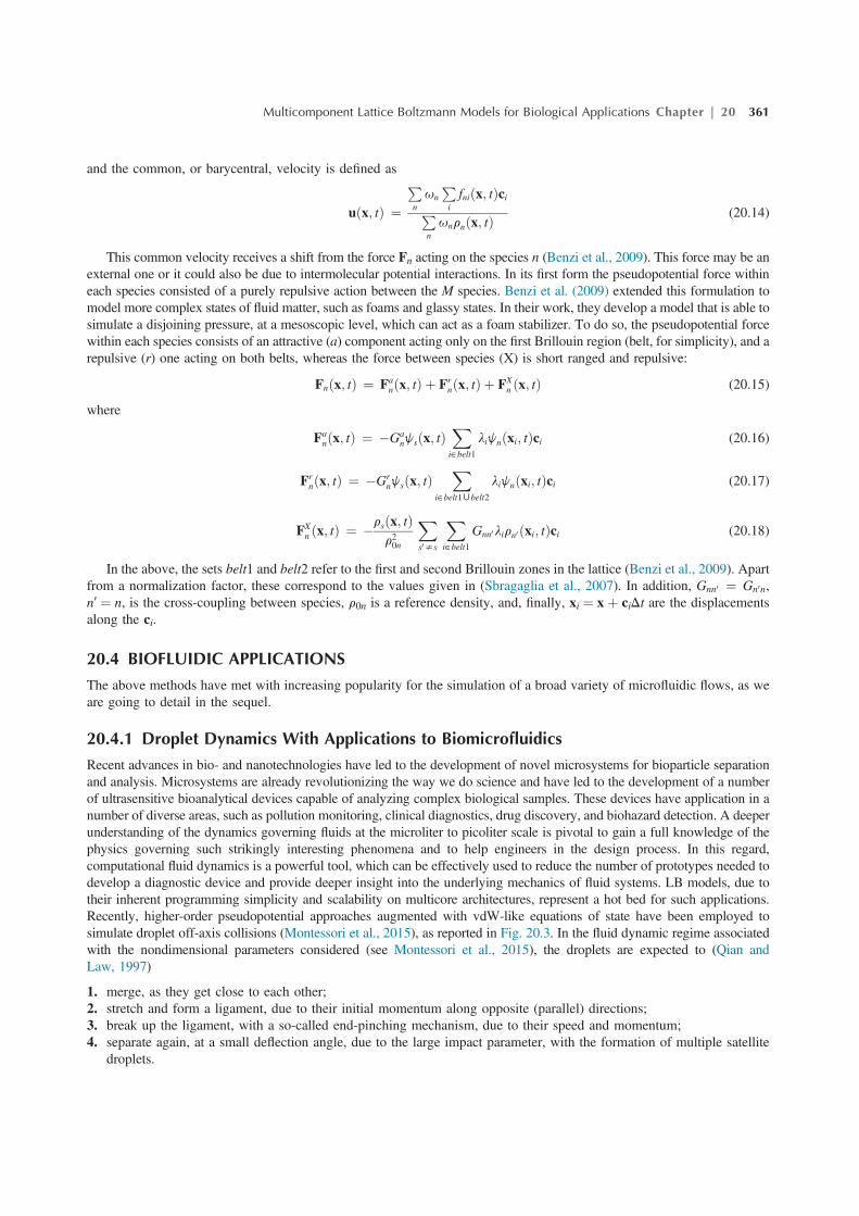
Recent advances in bio- and nanotechnologies have led to the development of novel microsystems for bioparticle separationand analysis. Microsystems are already revolutionizing the way we do science and have led to the development of a numberof ultrasensitive bioanalytical devices capable of analyzing complex biological samples. These devices have application in anumber of diverse areas, such as pollution monitoring, clinical diagnostics, drug discovery, and biohazard detection. A deeperunderstanding of the dynamics governing fluids at the microliter to picoliter scale is pivotal to gain a full knowledge of thephysics governing such strikingly interesting phenomena and to help engineers in the design process. In this regard,computational fluid dynamics is a powerful tool, which can be effectively used to reduce the number of prototypes needed todevelop a diagnostic device and provide deeper insight into the underlying mechanics of fluid systems. LB models, due totheir inherent programming simplicity and scalability on multicore architectures, represent a hot bed for such applications.Recently, higher-order pseudopotential approaches augmented with vdW-like equations of state have been employed tosimulate droplet off-axis collisions (Montessori et al., 2015), as reported in Fig. 20.3. In the fluid dynamic regime associatedwith the nondimensional parameters considered (see Montessori et al., 2015), the droplets are expected to (Qian andLaw, 1997)

1. merge, as they get close to each other;2. stretch and form a ligament, due to their initial momentum along opposite (parallel) directions;3. break up the ligament, with a so-called end-pinching mechanism, due to their speed and momentum;4. separate again, at a small deflection angle, due to the large impact parameter, with the formation of multiple satellite

droplets.


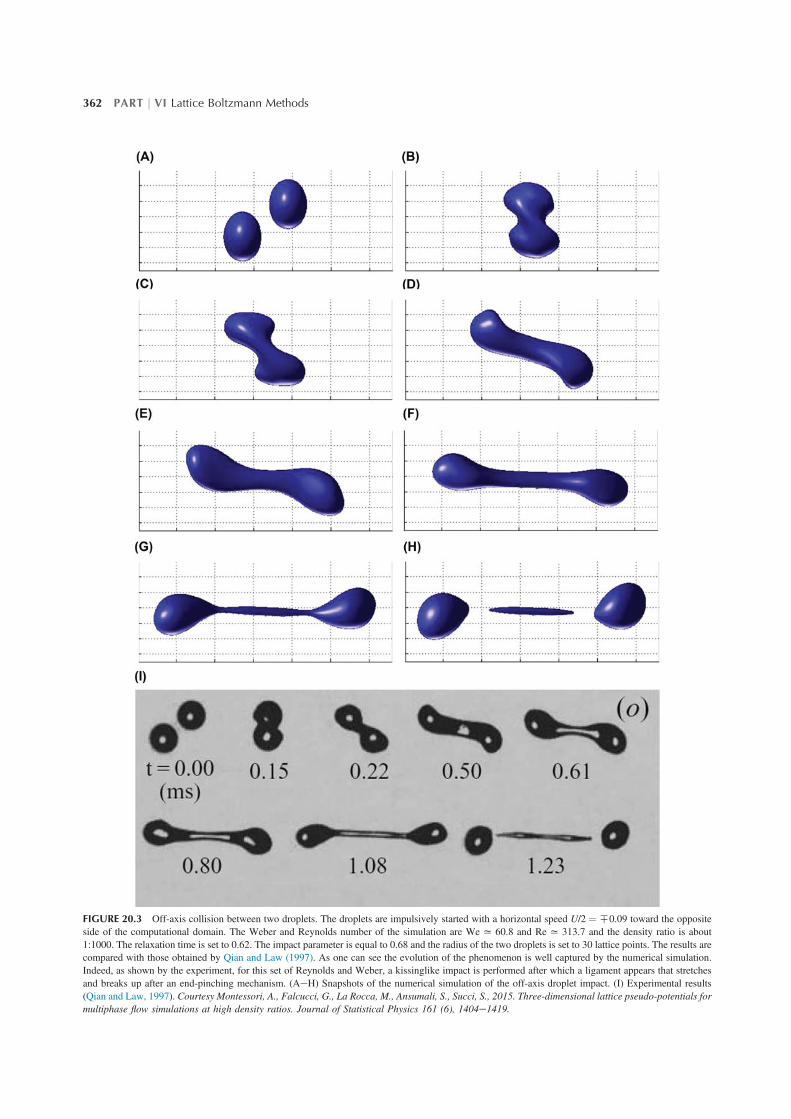
FIGURE 20.3 Off-axis collision between two droplets. The droplets are impulsively started with a horizontal speed U/2 ¼ H0.09 toward the oppositeside of the computational domain. The Weber and Reynolds number of the simulation are Wex 60.8 and Rex 313.7 and the density ratio is about1:1000. The relaxation time is set to 0.62. The impact parameter is equal to 0.68 and the radius of the two droplets is set to 30 lattice points. The results arecompared with those obtained by Qian and Law (1997). As one can see the evolution of the phenomenon is well captured by the numerical simulation.Indeed, as shown by the experiment, for this set of Reynolds and Weber, a kissinglike impact is performed after which a ligament appears that stretchesand breaks up after an end-pinching mechanism. (AeH) Snapshots of the numerical simulation of the off-axis droplet impact. (I) Experimental results(Qian and Law, 1997). Courtesy Montessori, A., Falcucci, G., La Rocca, M., Ansumali, S., Succi, S., 2015. Three-dimensional lattice pseudo-potentials formultiphase flow simulations at high density ratios. Journal of Statistical Physics 161 (6), 1404e1419.


This is precisely the sequence of events emerging from the simulation, as reported in Fig. 20.3. It is to be noted that awatereair-like system is here considered, i.e., the density ratio between the light and heavy fluid is x1000. Notwith-standing the large density ratio, the density contours appear very neat, with no sign of numerical debris at any stage of thiscomplex evolution, including the “critical” stages of merging and rupture. Moreover the evolution of the collision processis visually compared with the experiments carried out by Qian and Law. The results are in good agreement, at leastqualitatively. Indeed the kissinglike merging process and the consequent ligament stretching followed by the end-pinchingmechanism are well captured by the simulation.

Recently, Gupta and Sbragaglia (2014) investigated the effects of viscoelasticity on droplet dynamics and breakup inmicrofluidic in a T-junction geometry by means of a pseudopotentials multicomponent LB models coupled to a FENE-P(finitely extensible nonlinear elastic Peterlin) model (Gupta and Sbragaglia, 2014), employed to simulate the constitutiveequations for finite extensible nonlinear elastic dumbbells.

It is worth noting that T-junction-like devices are currently employed in medical diagnostics, i.e., for chemical(enzymatic and nonenzymatic) reactions and cell analysis. In addition, droplet digital polymerase chain reaction representsa promising way to diagnose and manage cancer, avoiding expensive and invasive traditional biopsies and enablingfrequent analysis of the tumor’s molecular profile. Thus, the understanding of the fluid dynamics processes in these devicesbecomes fundamental for the designer to create and control tiny droplets with great precision, for example maintaining aconsistent droplet size and frequency of droplet generation. Snapshot of the simulations for different values of the finiteextensibility parameter of the FENE-P equation is reported in Fig. 20.4.

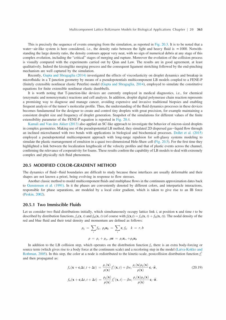
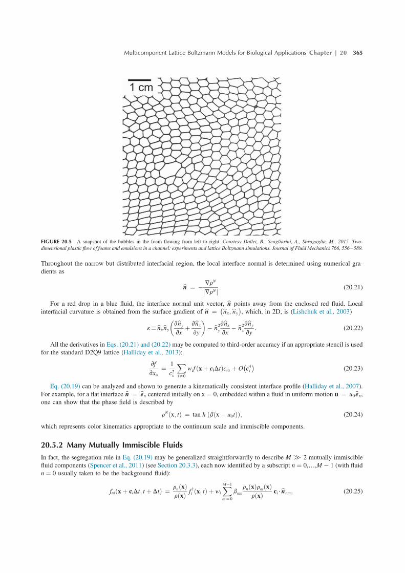
Kamali and Van den Akker (2013) also applied an SC-like approach to investigate the behavior of micron-sized dropletsin complex geometries. Making use of the pseudopotential LB method, they simulated 2D dispersed gaseliquid flow throughan inclined microchannel with two bends with applications in biological and biochemical processes. Dollet et al. (2015)employed a pseudopotential multicomponent approach with long-range repulsion for soft-glassy systems modeling tosimulate the plastic rearrangement of emulsion in a quasi two-dimensional Hele-Shaw cell (Fig. 20.5). For the first time theyhighlighted a link between the localization lengthscale of the velocity profiles and that of plastic events across the channel,confirming the relevance of cooperativity for foams. These results confirm the capability of LB models to deal with extremelycomplex and physically rich fluid phenomena.

20.5 MODIFIED COLOR-GRADIENT METHOD

The dynamics of fluidefluid boundaries are difficult to study because these interfaces are usually deformable and theirshapes are not known a priori, being evolving in response to flow stresses.

Another classic method to model multicomponent fluids and multiphase flows in the continuum approximation dates backto Gunstensen et al. (1991). In it the phases are conveniently denoted by different colors, and interparticle interactions,responsible for phase separations, are modeled by a local color gradient, which is taken to give rise to an IB force(Peskin, 2002).

20.5.1 Two Immiscible Fluids

Let us consider two fluid distributions initially, which simultaneously occupy lattice link i, at position x and time t to bedescribed by distribution functions, fri(x, t) and fbi(x, t) (of course with fi(x,t) ¼ fri(x, t) þ fbi(x, t)). The nodal density of thered and blue fluid and their total density and momentum are defined as follows:

rk ¼Xi

fki; rkuk ¼Xi

ci fki k ¼ r; b

r ¼ rr þ rb; ru ¼ rrur;þrbub

In addition to the LB collision step, which operates on the distribution function fi, there is an extra body-forcing orsource term (which gives rise to a body force at the continuum scale) and a recoloring step in the model (Latva-Kokko andRothman, 2005). In this step, the color at a node is redistributed to the kinetic-scale, postcollision distribution function f yiand then propagated as:

friðx þ ciDt; t þ DtÞ ¼ rrðxÞrðxÞ f yi ðx; tÞ þ bwi

rrðxÞrbðxÞrðxÞ ci$bn; (20.19)

fbiðx þ ciDt; t þ DtÞ ¼ rbðxÞrðxÞ f yi ðx; tÞ � bwi

rrðxÞrbðxÞrðxÞ ci$bn.


Clearly, the above rule represents a balance between dispersion of color (first term) and its preferential redirection to alattice region dominated by like color. The latter process is controlled by the segregation parameter b, discussed shortly. Asa consequence of using the rule in Eq. (20.19), together with an appropriate IB force, a drop of red fluid will spontaneouslyform from an initially uniform mixture of red and blue fluid. In Eq. (20.19) the continuum scale interface normal bn isdetermined as follows. The local phase field is (Halliday et al., 2007)

rNðx; tÞ ¼ rrðx; tÞ � rbðx; tÞrrðx; tÞ þ rbðx; tÞ

. (20.20)

Surfaces of constant rN value define the shape of the interfacial region with the surface rN ¼ 0 its center. Regions of thelattice characterized by rN ¼ �1 are considered to contain pure, bulk fluids. Interfacial fluid occupies regions where jrNj < 1.

FIGURE 20.4 Droplet formation in T-junction geometries. Panels (AeD) illustrate the squeezing regime at Ca ¼ 0.0026: the fluid thread enters andobstructs the main channel and breakup is mainly driven by the pressure buildup upstream of the emerging thread. Both the dynamics of breakup and thescaling of the sizes of droplets are influenced weakly by viscous forces. Panels (EeH) show typical features of the dripping regime at Ca ¼ 0.013: thebreakup process starts to be influenced by the shear forces, although the thread still occupies a significant portion of the main channel. This results insmaller droplets formed downstream of the T-junction. Courtesy Gupta, A., Sbragaglia, M., 2016. A lattice Boltzmann study of the effects of viscoelasticityon droplet formation in microfluidic cross-junctions. The European Physical Journal E 39 (1), 1e15.


Throughout the narrow but distributed interfacial region, the local interface normal is determined using numerical gra-dients as

bn ¼ � VrN

jVrN j . (20.21)

For a red drop in a blue fluid, the interface normal unit vector, bn points away from the enclosed red fluid. Localinterfacial curvature is obtained from the surface gradient of bn ¼ �bnx; bny�, which, in 2D, is (Lishchuk et al., 2003)

khbnxbny

�vbny

vxþ vbnx

vy

�� bn2

y

vbnx

vx� bn2

x

vbny

vy. (20.22)

All the derivatives in Eqs. (20.21) and (20.22) may be computed to third-order accuracy if an appropriate stencil is usedfor the standard D2Q9 lattice (Halliday et al., 2013):

vf

vxa¼ 1

c2s

Xis0

wif ðx þ ciDtÞcia þ O�c4i�

(20.23)

Eq. (20.19) can be analyzed and shown to generate a kinematically consistent interface profile (Halliday et al., 2007).For example, for a flat interface bn ¼ bex centered initially on x ¼ 0, embedded within a fluid in uniform motion u ¼ u0bex,one can show that the phase field is described by

rNðx; tÞ ¼ tan h ðbðx � u0tÞÞ; (20.24)

which represents color kinematics appropriate to the continuum scale and immiscible components.

20.5.2 Many Mutually Immiscible Fluids

In fact, the segregation rule in Eq. (20.19) may be generalized straightforwardly to describe M [ 2 mutually immisciblefluid components (Spencer et al., 2011) (see Section 20.3.3), each now identified by a subscript n ¼ 0,.,M � 1 (with fluidn ¼ 0 usually taken to be the background fluid):

fniðx þ ciDt; t þ DtÞ ¼ rnðxÞrðxÞ f yi ðx; tÞ þ wi

XM�1

m¼ 0

bnm

rnðxÞrmðxÞrðxÞ ci$bnnm; (20.25)

FIGURE 20.5 A snapshot of the bubbles in the foam flowing from left to right. Courtesy Dollet, B., Scagliarini, A., Sbragaglia, M., 2015. Two-dimensional plastic flow of foams and emulsions in a channel: experiments and lattice Boltzmann simulations. Journal of Fluid Mechanics 766, 556e589.


where the colored densities are defined as follows:

rn ¼Xi

fni; r ¼XM�1

n¼ 0

rn (20.26)

and a set of phase fields and associated gradients define the interfacial normals:

rNnmðx; tÞ ¼ rnðx; tÞ � rmðx; tÞrnðx; tÞ þ rmðx; tÞ

; bnnm ¼ � VrNnm��VrNnm�� . (20.27)

Note that it follows from the definition of the phase field thatbnnm ¼ �bnmn;

which means that color mass is conserved in Eq. (20.25). Now, if one makes additional assumptions regarding the absolutenumber of different fluids, which can be present at any lattice node, memory and execution speed scale only weakly withM, allowing for practical simulation of many, mutually immiscible drops or, indeed, vesicles (Dupin et al., 2004).

We defer further discussion of the application of this method to cellular-scale blood flow until we have accounted forthe method by which the dynamics of a biological membrane may be encapsulated within multicomponent LBsimulation.

20.6 MODELING MEMBRANES AS FLUIDeFLUID INTERFACES

Correct interfacial kinematics arise from the segregation step previously considered: specifically, a kinematic property ofmutual impenetrability emerges from the postcollision color segregation rules of the previous section. What we must nowconsider is the associated physical dynamics.

Generally, a spatially variable IB force distribution is applied to interfacial fluid (i.e., to regions of the lattice withjrNj < 1) to recover target dynamic boundary conditions. A simple example is provided by the continuum scale forcedistribution F ¼ 1

2 skVrN , which generates a Laplace pressure step of magnitude sk between the separated bulk fluids

(Lishchuk et al., 2003), along with a no-traction condition on tangential stress.In this section, we consider a more complex class of interfaces such as closed membranes, which are defined as

deformable boundaries separating two immiscible bulk fluids, each having conserved cross-sectional area. The enclosedliquid and membrane together form a vesicle. Unlike other interfacial problems where the area between the phases mayincrease or decrease, in the vesicle the total membrane or interface area is preserved, there being no mass exchangebetween the bilayer and the surrounding bulk fluid. However, like purely liquideliquid boundaries, membranes can beregarded as an unsteady interface responsive to flow stresses between the segregated fluids.

On the foundation of the color-gradient model set out above, we have developed a Lishchuk-type force able to produceappropriate continuum scale membrane boundary conditions. Simulations that contain such a membrane achieve, e.g., acorrect vesicle conformation by deforming and mediating appropriate physical stresses between the interior and exteriorfluids. The detailed structure of a biological membrane’s cytoskeleton and lipid bilayer is invisible at the continuum scale,so we adapt the approach of Kaoui et al. (2008) and postulate that interfacial fluid possesses properties representative of themembrane mechanics namely (1) preferred local curvature, (2) bending rigidity, (3) adjusted compressibility properties,(4) interfacial tension, and (5) conserved global length of the interfacial fluid. A representative force distribution derivesfrom the variational derivative of an expression for overall membrane free energy incorporating effects (1)e(5) (Hallidayet al., 2013). This force distribution is a normally directed, weighted fluid body force density acting only in the boundaryregion between the two fluids, i.e., on interfacial fluid:

F ¼ 12VrN

k

�s � a

�1 � l

l0

�� b

2k�k2 � k20

�� bv2k

vs2

. (20.28)

In the above, s denotes distance measured along the direction of the membrane, 12Vr

N is a weight (Lishchuk et al.,2003), k(k0) the (preferred) interfacial curvature, a the interfacial compressibility, s an interfacial tension further discussedbelow, l(l0) the (reference) length of the interface, and b its bending rigidity. Length l is maintained close to l0 by allowing

its value to modulate an effective interfacial tension s � a�1 � l

l0

�. That is, using that force density in Eq. (20.28), it

results in an equilibrium shape, which is consistent with a constant enclosed volume, membrane cross-sectional area(length in 2D), membrane preferred curvature, and interfacial tension, which may nevertheless be deformed when external


traction is applied, as the embedding fluid flows. Note that the constraint of constant vesicle volume is automatic as longas the enclosed fluid is incompressible and the parameterization of the membrane is direct. By selecting appropriateparameters, the deflation and deformability of vesicles may be readily adjusted (Halliday et al., 2013).

It is necessary briefly to consider how a spatially variable body force may be applied in LB simulation. The membraneforce in Eq. (20.28) is applied as an external force density to what is effectively a single lattice fluid described by kinetic-scale distribution function fi ¼ fri þ fbi. Doolen et al. (1998) and Guo et al. (2002) generalized the lattice BhatnagareGrosseKrook model, originally devised by Qian et al. (1992), to describe lattice fluid subject to a known, spatially variableexternal force density, F. Collision and forcing of the distribution function expressed in Eq. (20.1) may be straightfor-wardly reexpressed as

f yi ¼ f ð0Þi ðr; ruÞ þ ð1 � uÞf ð1Þi ðVr;.vxuy.;FÞ þ Fiðu;F; uÞ; (20.29)

where, recall, the dagger superscript indicates a postcollision, prepropagation quantity, and f ð0Þi ðr; uÞ denotes theequilibrium distribution function (Succi, 2001), and the source term, Fi, is

Fi ¼ wi

�1 � u

2

��ci � uc2s

þ ðci$uÞðciÞc4s

�$F; (20.30)

where all symbols have their usual meaning. Importantly, in the presence of an external force F, the value of the fluidvelocity depends on that external force (Guo et al., 2002):

u ¼ 1r

Xi

fici þ 12r

F. (20.31)

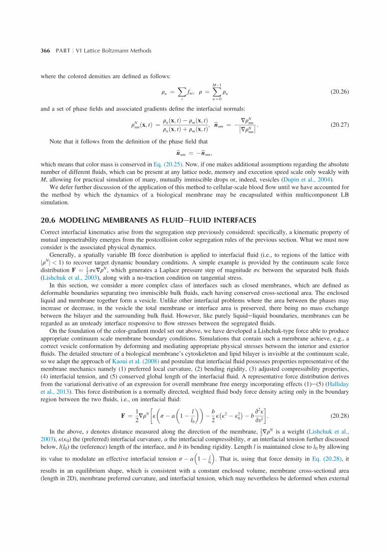
We return to this matter shortly. In the method outlined so far, all the dynamics and kinematics of the multifluid systemof plasma and vesicle(s) is embedded within (1) force distribution and (2) the fluids’ phase field. The method requires no setof constrained Lagrangian points to indicate the location of any of its potentially many interfaces (Halliday et al., 2013), andit inherits all the advantages of computational scaling with the number of immiscible components (i.e., vesicles) outlined inSection 20.5.2. Hence, little additional expense is incurred as the number of simulated vesicles increases beyond N ¼ 5, toproduce data such as that in Fig. 20.6. In the system represented there, there are>50 vesicles at representative concentrationc ¼ 0.42, with a range of deflations. A pressure gradient is applied to the system (regions of low (high) relative pressure arerendered blue (red)) and all the vesicles advect, deform, and order in response to the flow generated by the pressure gradientand the physics of their membranes. Simulation details may be found in the figure caption.

Although the data of Fig. 20.6 represent an efficient numerical solution to a very complex flow containing manyinteracting vesicles at high volume fraction, each vesicle shape evolves with the global membrane length (only) conserved.Implicitly, the constraint of global length conservation allows for different rates of strain in different membrane (interfacialfluid) regions, which in turn allows a variation of its tangential velocity. Such motion is only acceptable for a liquid drop.Put another way, the physical effect of uniform tangential motion (tank-treading motion) in the vesicle membrane is notrecovered.

FIGURE 20.6 A snapshot of pressure driven flow of multiple vesicles in a channel with a constriction at Re ¼ 30. Solid walls bound the domain, usingthe “link bounce-back method” (Succi, 2001). The pressure boundaries are implemented following Kim and Pitsch (2007). An exactly incompressibleD2Q9 lattice BhatnagareGrosseKrook model was used with vesicles’ properties as follows, all expressed in lattice units: bending rigidity b ¼ 0.55,surface tension s ¼ 0.008, membrane compressibility a ¼ 0.15, all fluids’ segregation parameters bnm ¼ 0.67, cn, m, and the membrane preferredcurvature k0 ¼ 0. For the almost-circular (low deflation) vesicle preferred length l0 ¼ 254 and its initial lattice area was 5153. For the 58 deflated vesicles,preferred length was l0 ¼ 224 and their initial area was 2706. The velocity field has been initialized at rest, u ¼ 0 and the snapshot of the flowconfiguration was taken at time step t ¼ 4444800. The overall simulation lattice is of size 999 � 297.


It was soon found that the method described so far must be enhanced if modalities associated with local incompressibilityof membrane length elements are to be recovered from individual vesicles’ fluid dynamics. We have recently introducedadditional normal and tangential forces to encapsulate such effects. Enhanced dynamics is accomplished by adding to thebody force density in expression (20.28) an additional contribution with a tangential component (Halliday et al., 2016):

F0 ¼ 12jVrN j

�kεkbn þ k

vε

vsbt�; (20.32)

where ε is a fictitious Hookean membrane strain and k its associated spring constant. The membrane strain field iscomputed from an explicit scheme solution of the equation:

vε

vt¼ vut

vs� ux

vε

vx� uy

vε

vy; (20.33)

where ut is the local tangential velocity of the membrane. Upwinding is necessary to compute the derivatives in theright-hand side. Unfortunately, the solution ε of Eq. (20.33) is dependent on u, which means that the correction forcein Eq. (20.32) inherits a velocity dependence. Because Fʹ ¼ F(u), Eqs. (20.31)e(20.33) must be solved by an iterativeprocedure (Halliday et al., 2016), to determine u and Fʹ.

Despite this elaborate procedure, the inclusion of Fʹ introduces the tank-treading and tumbling behavior into themethod, even for the quite deflated, biconcave shapes corresponding to red blood cells, at least in two dimensions, as wediscuss this in the next section. In conclusion, notwithstanding the issue raised above, our approach dispenses entirely withthe need explicitly to track the membrane, removes all need for computationally expensive and intricate interface trackingand remeshing, is completely Eulerian, and, not least, represents a two-way coupled vesicle membrane and flow within anLB framework.

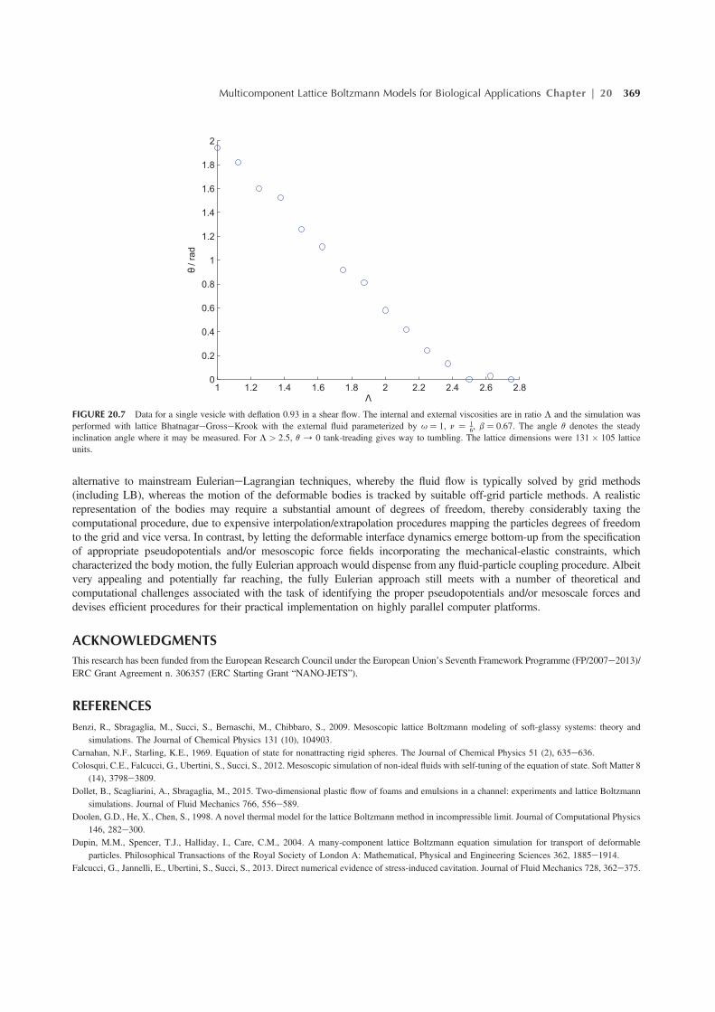
20.7 FLUID-FILLED VESICLES IN A SHEAR FLOW

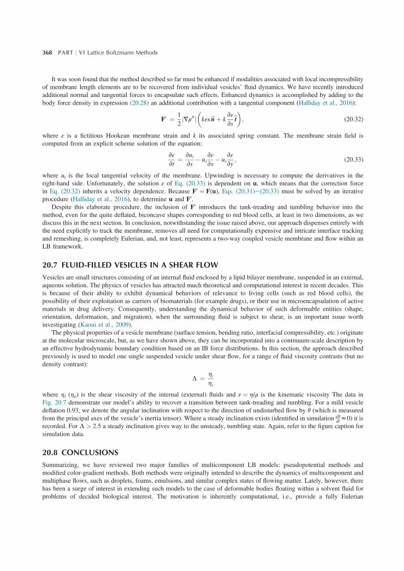
Vesicles are small structures consisting of an internal fluid enclosed by a lipid bilayer membrane, suspended in an external,aqueous solution. The physics of vesicles has attracted much theoretical and computational interest in recent decades. Thisis because of their ability to exhibit dynamical behaviors of relevance to living cells (such as red blood cells), thepossibility of their exploitation as carriers of biomaterials (for example drugs), or their use in microencapsulation of activematerials in drug delivery. Consequently, understanding the dynamical behavior of such deformable entities (shape,orientation, deformation, and migration), when the surrounding fluid is subject to shear, is an important issue worthinvestigating (Kaoui et al., 2009).

The physical properties of a vesicle membrane (surface tension, bending ratio, interfacial compressibility, etc.) originateat the molecular microscale, but, as we have shown above, they can be incorporated into a continuum-scale description byan effective hydrodynamic boundary condition based on an IB force distributions. In this section, the approach describedpreviously is used to model one single suspended vesicle under shear flow, for a range of fluid viscosity contrasts (but nodensity contrast):

L ¼ hi

he

where hi (he) is the shear viscosity of the internal (external) fluids and n ¼ h/r is the kinematic viscosity The data inFig. 20.7 demonstrate our model’s ability to recover a transition between tank-treading and tumbling. For a mild vesicledeflation 0.93, we denote the angular inclination with respect to the direction of undisturbed flow by q (which is measuredfrom the principal axes of the vesicle’s inertia tensor). Where a steady inclination exists (identified in simulation dq

dtz0) it isrecorded. For L > 2.5 a steady inclination gives way to the unsteady, tumbling state. Again, refer to the figure caption forsimulation data.

20.8 CONCLUSIONS

Summarizing, we have reviewed two major families of multicomponent LB models: pseudopotential methods andmodified color-gradient methods. Both methods were originally intended to describe the dynamics of multicomponent andmultiphase flows, such as droplets, foams, emulsions, and similar complex states of flowing matter. Lately, however, therehas been a surge of interest in extending such models to the case of deformable bodies floating within a solvent fluid forproblems of decided biological interest. The motivation is inherently computational, i.e., provide a fully Eulerian


alternative to mainstream EulerianeLagrangian techniques, whereby the fluid flow is typically solved by grid methods(including LB), whereas the motion of the deformable bodies is tracked by suitable off-grid particle methods. A realisticrepresentation of the bodies may require a substantial amount of degrees of freedom, thereby considerably taxing thecomputational procedure, due to expensive interpolation/extrapolation procedures mapping the particles degrees of freedomto the grid and vice versa. In contrast, by letting the deformable interface dynamics emerge bottom-up from the specificationof appropriate pseudopotentials and/or mesoscopic force fields incorporating the mechanical-elastic constraints, whichcharacterized the body motion, the fully Eulerian approach would dispense from any fluid-particle coupling procedure. Albeitvery appealing and potentially far reaching, the fully Eulerian approach still meets with a number of theoretical andcomputational challenges associated with the task of identifying the proper pseudopotentials and/or mesoscale forces anddevises efficient procedures for their practical implementation on highly parallel computer platforms.

ACKNOWLEDGMENTS

This research has been funded from the European Research Council under the European Union’s Seventh Framework Programme (FP/2007e2013)/ERC Grant Agreement n. 306357 (ERC Starting Grant “NANO-JETS”).

REFERENCES

Benzi, R., Sbragaglia, M., Succi, S., Bernaschi, M., Chibbaro, S., 2009. Mesoscopic lattice Boltzmann modeling of soft-glassy systems: theory andsimulations. The Journal of Chemical Physics 131 (10), 104903.

Carnahan, N.F., Starling, K.E., 1969. Equation of state for nonattracting rigid spheres. The Journal of Chemical Physics 51 (2), 635e636.Colosqui, C.E., Falcucci, G., Ubertini, S., Succi, S., 2012. Mesoscopic simulation of non-ideal fluids with self-tuning of the equation of state. Soft Matter 8

(14), 3798e3809.

Dollet, B., Scagliarini, A., Sbragaglia, M., 2015. Two-dimensional plastic flow of foams and emulsions in a channel: experiments and lattice Boltzmannsimulations. Journal of Fluid Mechanics 766, 556e589.

Doolen, G.D., He, X., Chen, S., 1998. A novel thermal model for the lattice Boltzmann method in incompressible limit. Journal of Computational Physics146, 282e300.

Dupin, M.M., Spencer, T.J., Halliday, I., Care, C.M., 2004. A many-component lattice Boltzmann equation simulation for transport of deformableparticles. Philosophical Transactions of the Royal Society of London A: Mathematical, Physical and Engineering Sciences 362, 1885e1914.

Falcucci, G., Jannelli, E., Ubertini, S., Succi, S., 2013. Direct numerical evidence of stress-induced cavitation. Journal of Fluid Mechanics 728, 362e375.

1 1.2 1.4 1.6 1.8 2 2.2 2.4 2.6 2.80

0.2

0.4

0.6

0.8

1

1.2

1.4

1.6

1.8

2

Λ

θ/rad

FIGURE 20.7 Data for a single vesicle with deflation 0.93 in a shear flow. The internal and external viscosities are in ratio L and the simulation wasperformed with lattice BhatnagareGrosseKrook with the external fluid parameterized by u ¼ 1, n ¼ 1

6, b ¼ 0.67. The angle q denotes the steadyinclination angle where it may be measured. For L > 2.5, q / 0 tank-treading gives way to tumbling. The lattice dimensions were 131 � 105 latticeunits.


Grunau, D., Chen, S., Eggert, K., 1989-1993. A lattice Boltzmann model for multiphase fluid flows. Physics of Fluids A: Fluid Dynamics 5 (10),

2557e2562.Gunstensen, A.K., Rothman, D.H., Zaleski, S., Zanetti, G., 1991. Lattice Boltzmann model of immiscible fluids. Physical Review A 43 (8), 4320.Guo, Z., Zheng, C., Shi, B., April 2002. Discrete lattice effects on the forcing term in the lattice Boltzmann method. Physical Review E 65, 046308.

Gupta, A., Sbragaglia, M., 2014. Deformation and breakup of viscoelastic droplets in confined shear flow. Physical Review E 90 (2), 023305.Gupta, A., Sbragaglia, M., 2016. A lattice Boltzmann study of the effects of viscoelasticity on droplet formation in microfluidic cross-junctions. The

European Physical Journal E 39 (1), 1e15.Halliday, I., Hollis, A.P., Care, C.M., 2007. Lattice Boltzmann algorithm for continuum multicomponent flow. Physical Review E 76 (2), 026708.

Halliday, I., Lishchuk, S.V., Spencer, T.J., Pontrelli, G., Care, C.M., 2013. Multiple-component lattice Boltzmann equation for fluid-filled vesicles in flow.Physical Review E 87, 023307.

Halliday, I., Lishchuk, S.V., Spencer, T.J., Pontrelli, G., Evans, P.C., 2016. Local membrane length conservation in two-dimensional vesicle simulation

using a multicomponent lattice Boltzmann equation method. Physical Review E 94, 023306.Kamali, M.R., Van den Akker, H.E.A., 2013. Simulating gas-liquid flows by means of a pseudopotential lattice Boltzmann method. Industrial and

Engineering Chemistry Research 52 (33), 11365e11377.

Kaoui, B., Ristow, G.H., Cantat, I., Misbah, C., Zimmermann, W., February 2008. Lateral migration of a two-dimensional vesicle in unbounded poiseuilleflow. Physical Review E 77, 021903.

Kaoui, B., Biros, G., Misbah, C., October 2009. Why do red blood cells have asymmetric shapes even in a symmetric flow? Physical Review Letters 103,

188101.Kim, S.H., Pitsch, H., 2007. A generalized periodic boundary condition for lattice Boltzmann method simulation of a pressure driven flow in a periodic

geometry. Physics of Fluids 19 (10), 108101.Körner, C., Thies, M., Hofmann, T., Thürey, N., Rüde, U., 2005. Lattice Boltzmann model for free surface flow for modeling foaming. Journal of

Statistical Physics 121 (1e2), 179e196.Lallemand, P., Luo, L.-S., Peng, Y., 2007. A lattice Boltzmann front-tracking method for interface dynamics with surface tension in two dimensions.

Journal of Computational Physics 226 (2), 1367e1384.

Latva-Kokko, M., Rothman, D.H., 2005. Diffusion properties of gradient-based lattice Boltzmann models of immiscible fluids. Physical Review E 71 (5),056702.

Lishchuk, S.V., Care, C.M., Halliday, I., 2003. Lattice Boltzmann algorithm for surface tension with greatly reduced microcurrents. Physical Review E 67,

036701.Montessori, A., Falcucci, G., La Rocca, M., Ansumali, S., Succi, S., 2015. Three-dimensional lattice pseudo-potentials for multiphase flow simulations at

high density ratios. Journal of Statistical Physics 161 (6), 1404e1419.Montessori, A., Prestininzi, P., La Rocca, M., Falcucci, G., Succi, S., Kaxiras, E., 2016. Effects of Knudsen diffusivity on the effective reactivity of

nanoporous catalyst media. Journal of Computational Science 17 (Part 2), 377e383.Orlandini, E., Swift, M.R., Yeomans, J.M., 1995. A lattice Boltzmann model of binary-fluid mixtures. Europhysics Letters 32 (6), 463.Peskin, C.S., 2002. The immersed boundary method. Acta Numerica 11, 479e517.

Qian, Y.H., d’Humieres, D., Lallemand, P., 1992. Lattice BGK models for Navier-Stokes equation. Europhysics Letters 17 (6), 479.Qian, J., Law, C.K., 1997. Regimes of coalescence and separation in droplet collision. Journal of Fluid Mechanics 331, 59e80.Qin, R.S., June 2006. Mesoscopic interparticle potentials in the lattice Boltzmann equation for multiphase fluids. Physical Review E 73, 066703. http://

dx.doi.org/10.1103/PhysRevE.73.066703. URL: http://link.aps.org/doi/10.1103/PhysRevE.73.066703.Rothman, D.H., Keller, J.M., 1988. Immiscible cellular-automaton fluids. Journal of Statistical Physics 52 (3e4), 1119e1127.Swift, M.R., Osborn, W.R., Yeomans, J.M., 1995. Lattice Boltzmann simulation of nonideal fluids. Physical Review Letters 75 (5), 830.

Sbragaglia, M., Benzi, R., Biferale, L., Succi, S., Sugiyama, K., Toschi, F., 2007. Generalized lattice Boltzmann method with multirange pseudopotential.Physical Review E 75 (2), 026702.

Shan, X., 2006. Analysis and reduction of the spurious current in a class of multiphase lattice Boltzmann models. Physical Review E 73 (4), 047701.Shan, X., Chen, H., 1993. Lattice Boltzmann model for simulating flows with multiple phases and components. Physical Review E 47 (3), 1815.

Spencer, T.J., Halliday, I., Care, C.M., 2011. A local lattice Boltzmann method for multiple immiscible fluids and dense suspensions of drops. Philo-sophical Transactions of the Royal Society of London A: Mathematical, Physical and Engineering Sciences 369 (1944), 2255e2263.

Succi, S., 2001. The Lattice Boltzmann Equation for Fluid Dynamics and Beyond. Oxford University Press.

Succi, S., 2015. Lattice Boltzmann 2038. Europhysics Letters 109 (5), 50001.Wolfram, S., 1986. Cellular automaton fluids 1: basic theory. Journal of Statistical Physics 45 (3e4), 471e526.Yuan, P., Schaefer, L., 2006. Equations of state in a lattice Boltzmann model. Physics of Fluids 18 (4), 042101.


Documents

Numerical Methods and Advanced Simulation in …pontrell/pub/CERROLAZA_chapter20.pdfNumerical Methods and Advanced Simulation in Biomechanics and Biological Processes Edited by Miguel