Numerical method for the 2D simulation of the respiration · Numerical method for the 2D simulation of the respiration ... Bertrand Maury, Driss Yakoubi. Numerical method for the

HAL Id: hal-00357943https://hal.archives-ouvertes.fr/hal-00357943

Submitted on 2 Feb 2009

HAL is a multi-disciplinary open accessarchive for the deposit and dissemination of sci-entific research documents, whether they are pub-lished or not. The documents may come fromteaching and research institutions in France orabroad, or from public or private research centers.

L’archive ouverte pluridisciplinaire HAL, estdestinée au dépôt et à la diffusion de documentsscientifiques de niveau recherche, publiés ou non,émanant des établissements d’enseignement et derecherche français ou étrangers, des laboratoirespublics ou privés.

Numerical method for the 2D simulation of therespiration

Anne Devys, Céline Grandmont, Bérénice Grec, Bertrand Maury, DrissYakoubi

To cite this version:Anne Devys, Céline Grandmont, Bérénice Grec, Bertrand Maury, Driss Yakoubi. Numerical methodfor the 2D simulation of the respiration. ESAIM: Proceedings, EDP Sciences, 2009, 28, pp.162-181.<10.1051/proc/2009045>. <hal-00357943>

https://hal.archives-ouvertes.fr/hal-00357943

https://hal.archives-ouvertes.fr

ESAIM: PROCEEDINGS, Vol. ?, 2009, 1-10

Editors: Will be set by the publisher

NUMERICAL METHOD FOR THE

2D SIMULATION OF THE RESPIRATION. ∗

A. Devys1, 2, C. Grandmont3, B. Grec4, B. Maury5 and D.Yakoubi3

Abstract. In this article we are interested in the simulation of the air flow in the bronchial tree.The model we use has already been described in [2] and is based on a three part description of therespiratory tract. This model leads, after time discretization, to a Stokes system with non standarddissipative boundary conditions that cannot be easily and directly implemented in most FEM software,in particular in FreeFEM++ [10]. The objective is here to provide a new numerical method that couldbe implemented in any softwares. After describing the method, we illustrate it by two-dimensionalsimulations.

Resume. Dans cet article nous nous interessons a la simulation du flux d’air dans l’arbre bronchique.Le modele que nous utilisons a deja ete decrit dans [2] et consiste en une description selon trois parties del’arbre respiratoire. Ce modele nous conduit, apres discretisation en temps, a un probleme de Stokesavec des conditions au bord dissipatives non usuelles qui ne peuvent etre implementees facilementet directement dans la plupart des logiciels utilisant la methode des elements finis, en particulierFreeFEM++ [10]. L’objectif ici, est d’apporter une methode de resolution implementable dans toutlogiciel EFM. Apres une description de la methode, nous l’illustrerons par des simulations 2D.

Introduction

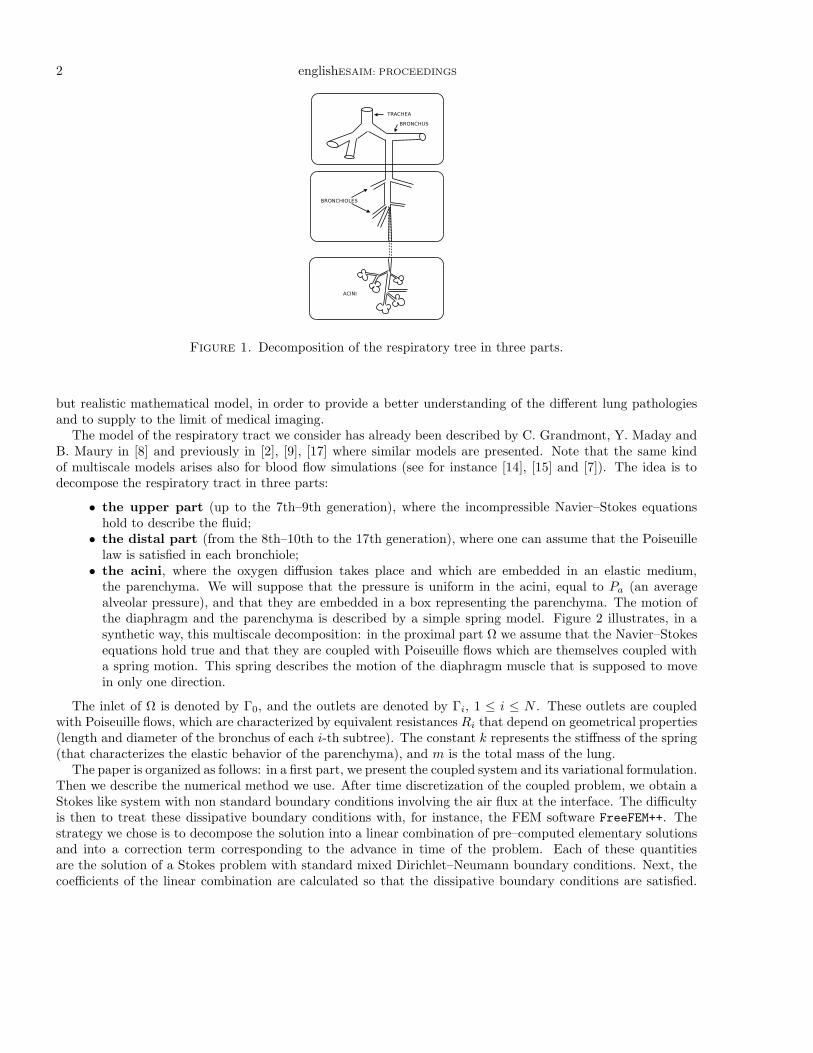
Breathing involves gas transport through the respiratory tract with its visible ends, nose and mouth. Thebronchial tree which ends in the alveoli is embedded in a viscoelastic tissue, the whole being enclosed belowby the diaphragm and laterally by the chest wall. The air movement is achieved by the displacement of thediaphragm and of the connective tissue framework of the lung (in the sequel we will talk about the parenchyma).The respiratory tract has a quite complex geometry: it is a tree composed by 23 generations which should beimplemented (see Fig. 1). At the time being, the distal airways from generation 9 cannot be visualized/segmentedby common medical imaging technologies for instance. Consequently it is necessary to elaborate some simple

∗ This work was partially funded by the ANR-08-JCJC-013-01 project headed by C.Grandmont.

1 UST Lille, Lab. P. Painleve, Cite Scientifique, F-59655 Villeneuve d’Ascq Cedex, France;e-mail: [email protected] INRIA Lille Nord Europe, SIMPAF Project team, B.P. 70478, F-59658 Villeneuve d’Ascq Cedex, France;3 INRIA Paris-Rocquencourt, REO Project team, BP 105, F-78153 Le Chesnay Cedex, France;e-mail: [email protected] & [email protected] Universite Claude Bernard Lyon 1, Institut C. Jordan, F-69622 Villeurbanne Cedex, France;e-mail: [email protected] Universite Paris-Sud, Laboratoire de mathematiques, Batiment 425, bureau 130, F-91405 Orsay cedex, France;e-mail: [email protected]

c© EDP Sciences, SMAI 2009

2 englishESAIM: PROCEEDINGS

Figure 1. Decomposition of the respiratory tree in three parts.

but realistic mathematical model, in order to provide a better understanding of the different lung pathologiesand to supply to the limit of medical imaging.

The model of the respiratory tract we consider has already been described by C. Grandmont, Y. Maday andB. Maury in [8] and previously in [2], [9], [17] where similar models are presented. Note that the same kindof multiscale models arises also for blood flow simulations (see for instance [14], [15] and [7]). The idea is todecompose the respiratory tract in three parts:

• the upper part (up to the 7th–9th generation), where the incompressible Navier–Stokes equationshold to describe the fluid;

• the distal part (from the 8th–10th to the 17th generation), where one can assume that the Poiseuillelaw is satisfied in each bronchiole;

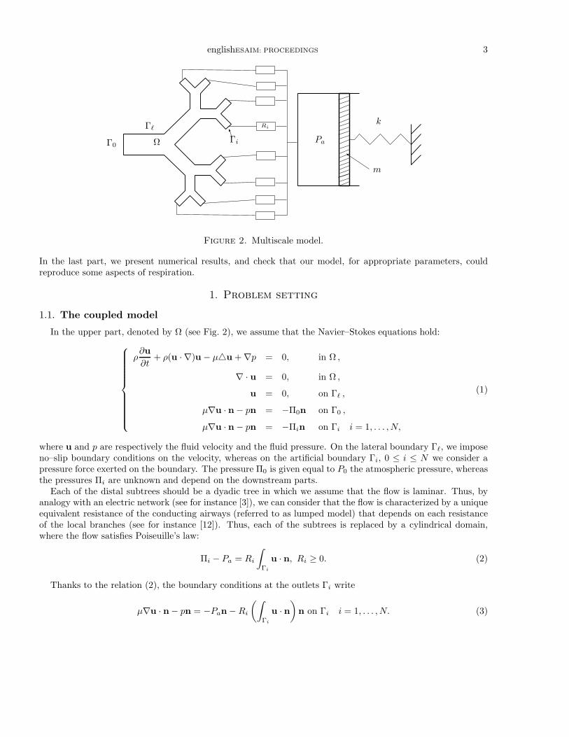
• the acini, where the oxygen diffusion takes place and which are embedded in an elastic medium,the parenchyma. We will suppose that the pressure is uniform in the acini, equal to Pa (an averagealveolar pressure), and that they are embedded in a box representing the parenchyma. The motion ofthe diaphragm and the parenchyma is described by a simple spring model. Figure 2 illustrates, in asynthetic way, this multiscale decomposition: in the proximal part Ω we assume that the Navier–Stokesequations hold true and that they are coupled with Poiseuille flows which are themselves coupled witha spring motion. This spring describes the motion of the diaphragm muscle that is supposed to movein only one direction.

The inlet of Ω is denoted by Γ0, and the outlets are denoted by Γi, 1 ≤ i ≤ N . These outlets are coupledwith Poiseuille flows, which are characterized by equivalent resistances Ri that depend on geometrical properties(length and diameter of the bronchus of each i-th subtree). The constant k represents the stiffness of the spring(that characterizes the elastic behavior of the parenchyma), and m is the total mass of the lung.

The paper is organized as follows: in a first part, we present the coupled system and its variational formulation.Then we describe the numerical method we use. After time discretization of the coupled problem, we obtain aStokes like system with non standard boundary conditions involving the air flux at the interface. The difficultyis then to treat these dissipative boundary conditions with, for instance, the FEM software FreeFEM++. Thestrategy we chose is to decompose the solution into a linear combination of pre–computed elementary solutionsand into a correction term corresponding to the advance in time of the problem. Each of these quantitiesare the solution of a Stokes problem with standard mixed Dirichlet–Neumann boundary conditions. Next, thecoefficients of the linear combination are calculated so that the dissipative boundary conditions are satisfied.

englishESAIM: PROCEEDINGS 3

Γ0 Ω

Γℓ

Γi

Ri

Pa

k

m

Figure 2. Multiscale model.

In the last part, we present numerical results, and check that our model, for appropriate parameters, couldreproduce some aspects of respiration.

1. Problem setting

1.1. The coupled model

In the upper part, denoted by Ω (see Fig. 2), we assume that the Navier–Stokes equations hold:

ρ∂u

∂t+ ρ(u · ∇)u − µu + ∇p = 0, in Ω ,

∇ · u = 0, in Ω ,

u = 0, on Γℓ ,

µ∇u · n − pn = −Π0n on Γ0 ,

µ∇u · n − pn = −Πin on Γi i = 1, . . . , N,

(1)

where u and p are respectively the fluid velocity and the fluid pressure. On the lateral boundary Γℓ, we imposeno–slip boundary conditions on the velocity, whereas on the artificial boundary Γi, 0 ≤ i ≤ N we consider apressure force exerted on the boundary. The pressure Π0 is given equal to P0 the atmospheric pressure, whereasthe pressures Πi are unknown and depend on the downstream parts.

Each of the distal subtrees should be a dyadic tree in which we assume that the flow is laminar. Thus, byanalogy with an electric network (see for instance [3]), we can consider that the flow is characterized by a uniqueequivalent resistance of the conducting airways (referred to as lumped model) that depends on each resistanceof the local branches (see for instance [12]). Thus, each of the subtrees is replaced by a cylindrical domain,where the flow satisfies Poiseuille’s law:

Πi − Pa = Ri

∫

Γi

u · n, Ri ≥ 0. (2)

Thanks to the relation (2), the boundary conditions at the outlets Γi write

µ∇u · n− pn = −Pan− Ri

(∫

Γi

u · n

)

n on Γi i = 1, . . . , N. (3)


These are non standard nonlocal boundary conditions that link the fluid stress tensor and its flux that arisealso in blood flow modelling (see [7]). Note that they induce dissipation in the system (see [2]). We will callthis type of boundary conditions the natural dissipative boundary conditions. Next, the lung is enclosed in abox and one part of this box is connected to a spring that governs the diaphragm and parenchyma motion. Theequation satisfied by the position x of the diaphragm writes

mx = −kx + fext + PaS, (4)

where fext is the force developed by the diaphragm during inspiration and expiration. It will be the drivenforce of the respiration. In order to couple this simple ODE to the upper part of the model, we have to definefP that stands for the pressure force applied by the flow on the elastic medium. If we denote by S the surfaceof the moving box (corresponding to the diaphragm surface), we have

fP = PaS, (5)

thus

Pa =m

Sx +

k

Sx −

fext

S. (6)

Moreover, since we assume that the parenchyma is made of an incompressible medium, the flow volumevariation at the outlets is equal to the volume variation of the parenchyma box, thus we have

Sx =

N∑

i=1

∫

Γi

u · n. (7)

Note that since the flow is incompressible and since u = 0 on Γℓ, then

N∑

i=1

∫

Γi

u · n = −

∫

Γ0

u · n. (8)

Thus the coupled problem can be written as follows

ρ∂u

∂t+ ρ(u · ∇)u − µu + ∇p = 0 , in (0, T ) × Ω ,

∇ · u = 0 , in (0, T ) × Ω ,u = 0 , on (0, T )× Γℓ ,

µ∇u · n− pn = −P0n , on (0, T )× Γ0 ,

µ∇u · n− pn = −Pan− Ri

(∫

Γi

u · n

)

n , on (0, T )× Γi ,

i = 1 , . . . , N ,mx + kx = fext + SPa ,

Sx =

N∑

i=1

∫

Γi

u · n = −

∫

Γ0

u · n.

(9)

This system of equations has to be completed by suitable initial conditions

(u, x, x)|t=0 = (u0, x0, x1), with

∇ · u0 = 0 , u0 = 0 on Γℓ , and Sx1 = −

∫

Γ0

u0 · n.(10)

One particularity of this system is that all the outlets Γi, 1 ≤ i ≤ N are coupled.


By setting p = p − Pa , according to (6) and since the total volume is preserved, i.e Sx = −

∫

Γ0

u · n, the

coupled system can be simplified as follows

ρ∂u

∂t+ ρ(u · ∇)u − µu + ∇p = 0 , in (0, T ) × Ω ,

∇ · u = 0 , in (0, T ) × Ω ,u = 0 , on (0, T )× Γℓ ,

µ∇u · n − pn = −P0n −fext

Sn−

m

S2

d

dt

(∫

Γ0

u · n

)

n

−k

S2

(∫ t

0

∫

Γ0

u · n − Sx0

)

n , on (0, T )× Γ0 ,

µ∇u · n − pn = −Ri

(∫

Γi

u · n

)

n , on (0, T )× Γi.

(11)

Consequently, the coupled system (9) reduces to the Navier–Stokes equations, with fluid pressure replaced bythe difference between fluid pressure and alveolar pressure, and with generalized natural dissipative boundaryconditions. Note that the incompressibility assumption is essential here.

Remark 1.1. We have used the relation

N∑

i=1

∫

Γi

u · n = −

∫

Γ0

u · n to simplify system (9), to decouple the

outlets Γi and obtain (11). Nevertheless all what will be done hereafter could also be done without using thisrelation.

1.2. Variational formulation

We introduce the following functional space V = v ∈ H1(Ω)d , ∇ · v = 0,v = 0 on Γℓ. Assuming that allthe unknowns are regular enough, we multiply the Navier–Stokes equations by a test–field v which vanishes onΓℓ, and the spring equation by −(1/S)

∫

Γ0

v · n. Using

x = x0 −1

S

∫ t

0

∫

Γ0

u · n,

we obtain

ρ

∫

Ω

∂tu · v + ρ

∫

Ω

(u · ∇)u · v + µ

∫

Ω

∇u : ∇v +N∑

i=1

Ri

(∫

Γi

u · n

)(∫

Γi

v · n

)

+m

S2

(∫

Γ0

∂tu · n

)(∫

Γ0

v · n

)

+k

S2

(∫ t

0

∫

Γ0

u · n

)(∫

Γ0

v · n

)

−

∫

Ω

p∇ · v + Pa

(

N∑

i=1

∫

Γi

v · n −

∫

Γ0

v · n

)

= −P0

∫

Γ0

v · n −fext

S

∫

Γ0

v · n +k

S2Sx0

(∫

Γ0

v · n

)

, ∀v ∈ H1(Ω)d with v|Γℓ= 0.

(12)

Next, considering test functions v that are divergence free (i.e v ∈ V ), we obtain a second variational formulationof the coupled problem (11)


ρ

∫

Ω

∂tu · v + ρ

∫

Ω

(u · ∇)u · v + µ

∫

Ω

∇u : ∇v +N∑

i=1

Ri

(∫

Γi

u · n

)(∫

Γi

v · n

)

+m

S2

(∫

Γ0

∂tu · n

)(∫

Γ0

v · n

)

+k

S2

(∫ t

0

∫

Γ0

u · n

)(∫

Γ0

v · n

)

= −P0

∫

Γ0

v · n −fext

S

∫

Γ0

v · n +k

Sx0

(∫

Γ0

v · n

)

, ∀v ∈ V.

(13)

Note that here, we have expressed all the quantities with the help of the fluid velocity. The velocity of the

spring can be simply recovered thanks to the identity Sx = −

∫

Γ0

u · n.

2. Numerical method

In this section we will first present the numerical method on a linear problem obtained by omitting theconvection terms. Then we will explain how it can be adapted to the general case.

2.1. The Stokes system

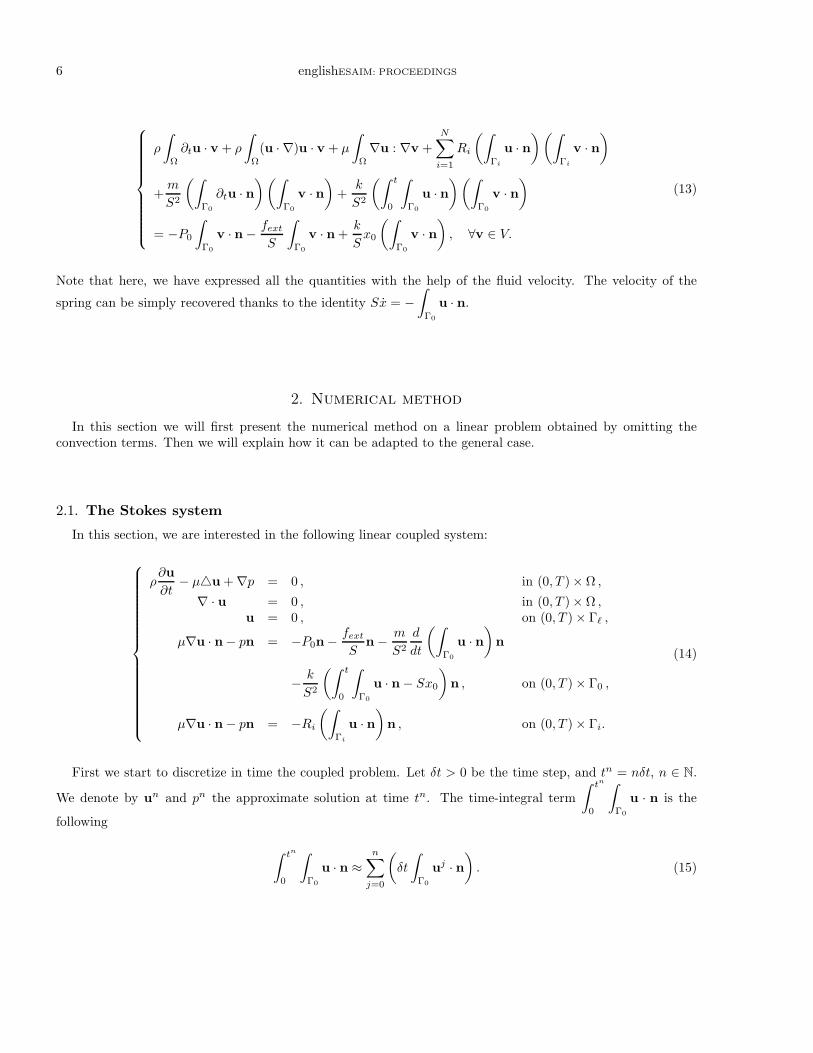
In this section, we are interested in the following linear coupled system:

ρ∂u

∂t− µu + ∇p = 0 , in (0, T )× Ω ,

∇ · u = 0 , in (0, T )× Ω ,u = 0 , on (0, T ) × Γℓ ,

µ∇u · n− pn = −P0n−fext

Sn −

m

S2

d

dt

(∫

Γ0

u · n

)

n

−k

S2

(∫ t

0

∫

Γ0

u · n− Sx0

)

n , on (0, T ) × Γ0 ,

µ∇u · n− pn = −Ri

(∫

Γi

u · n

)

n , on (0, T ) × Γi.

(14)

First we start to discretize in time the coupled problem. Let δt > 0 be the time step, and tn = nδt, n ∈ N.

We denote by un and pn the approximate solution at time tn. The time-integral term

∫ tn

0

∫

Γ0

u · n is the

following

∫ tn

0

∫

Γ0

u · n ≈n∑

j=0

(

δt

∫

Γ0

uj · n

)

. (15)


The time discretization reads as follows

ρun

δt− µun + ∇pn = ρ

un−1

δt, in Ω ,

∇ · un = 0 , in Ω ,

un = 0, on Γℓ ,

µ∇un · n− pnn = −

P0 +fn

ext

S−

kx0

S+

kδt

S2

n−1∑

j=0

(∫

Γ0

uj · n

)

−m

S2δt

(∫

Γ0

un−1 · n

)

n

−

(

m

S2δt−

kδt

S2

)(∫

Γ0

un · n

)

n , on Γ0 ,

µ∇un · n− pnn = −Ri

(∫

Γi

un · n

)

n , on Γi i = 1, . . . , N.

(16)In the sequel, we use the following notations

Fn = P0 +fn

ext

S−

kx0

S+

kδt

S2

n−1∑

j=0

(∫

Γ0

uj · n

)

−m

S2δt

(∫

Γ0

un−1 · n

)

(17)

and

Rδt0 =

m

S2δt−

kδt

S2. (18)

Note that Fn is known as soon as the velocities at the previous time steps have been computed. The problem(16) can then be written as

ρun


un−1

δt, in Ω ,

∇ · un = 0 , in Ω ,

un = 0, on Γℓ ,

µ∇un · n− pnn = −Fnn − Rδt0

(∫

Γ0

un · n

)

n , on Γ0 ,

µ∇un · n− pnn = −Ri

(∫

Γi

un · n

)

n , on Γi i = 1, . . . , N.

(19)

Consequently, after time discretization, we obtain a generalized Stokes problem with natural dissipative bound-ary conditions. These unusual boundary conditions coming from the resistance and the mass–spring time–discretization modify the standard bilinear forms associated to a Stokes problem with mixed Dirichlet–Neumannboundary conditions. In particular, if we consider a finite element discretization, they would couple all the de-gree of freedom at each outlet and change the finite elements matrix pattern associated to the velocity degreesof freedom. Consequently, they cannot be easily and directly implemented in a any FEM solver, for instance inFreeFEM++, without going deeply into the code.

To get rid of this difficulty, we use the following method. The objective is to reduce this problem with nonstandard boundary conditions to problems with Neumann and Dirichlet boundary conditions. The idea is topre–compute a set of solutions with Neumann boundary conditions on each Γi, and then to define the solutionas a linear combination of these solutions and of a correction term. This correction term solves also a Stokesproblem with standard boundary conditions, the coefficients of the linear combination being calculated so thatthe solution satisfies the dissipative boundary conditions.


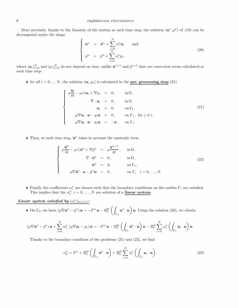
More precisely, thanks to the linearity of the system at each time step, the solution (un, pn) of (19) can bedecomposed under the shape

un = un +N∑

i=0

αni ui and

pn = pn +N∑

i=0

αni pi,

(20)

where (ui)Ni=0 and (pi)

Ni=0 do not depend on time, unlike un+1 and pn+1 that are correction terms calculated at

each time step:

• for all i = 0, . . .N , the solution (ui, pi) is calculated in the pre–processing step (21)

ρui

δt− µui + ∇pi = 0 , in Ω ,

∇ · ui = 0 , in Ω ,

ui = 0, onΓℓ ,

µ∇ui · n− pin = 0 , on Γj , for j 6= i ,

µ∇ui · n− pin = −n , on Γi.

(21)

• Then, at each time step, un takes in account the unsteady term

ρun


un−1

δt, in Ω ,

∇ · un = 0 , in Ω ,

un = 0, on Γℓ ,

µ∇un · n− pnn = 0 , on Γi i = 0, . . . , N.

(22)

• Finally the coefficients αni are chosen such that the boundary conditions on the outlets Γi are satisfied.

This implies that the αni , i = 0, . . . , N are solution of a linear system.

Linear system satisfied by (αni )0≤i≤N :

• On Γ0, we have (µ∇un − pn)n = −Fn n − Rδt0

(∫

Γ0

un · n

)

n. Using the relation (20), we obtain

(µ∇un − pn)n +

N∑

i=0

αni (µ∇ui − pi)n = −Fn n − Rδt

0

(∫

Γ0

un · n

)

n− Rδt0

N∑

i=0

αni

(∫

Γ0

ui · n

)

n.

Thanks to the boundary condition of the problems (21) and (22), we find

αn0 = Fn + Rδt

0

(∫

Γ0

un · n

)

+ Rδt0

N∑

i=0

αni

(∫

Γ0

ui · n

)

. (23)


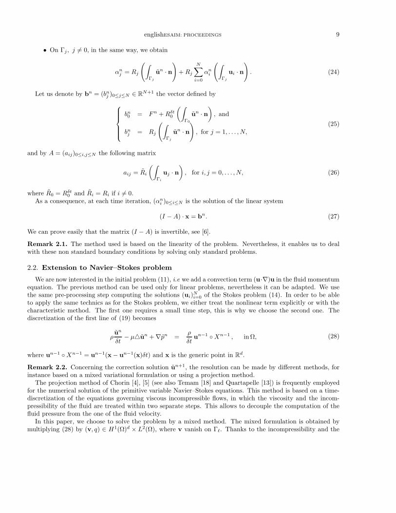
• On Γj , j 6= 0, in the same way, we obtain

αnj = Rj

(

∫

Γj

un · n

)

+ Rj

N∑

i=0

αni

(

∫

Γj

ui · n

)

. (24)

Let us denote by bn = (bnj )0≤j≤N ∈ R

N+1 the vector defined by

bn0 = Fn + Rδt

0

(∫

Γ0

un · n

)

, and

bnj = Rj

(

∫

Γj

un · n

)

, for j = 1, . . . , N,(25)

and by A = (aij)0≤i,j≤N the following matrix

aij = Ri

(∫

Γi

uj · n

)

, for i, j = 0, . . . , N, (26)

where R0 = Rδt0 and Ri = Ri if i 6= 0.

As a consequence, at each time iteration, (αni )0≤i≤N is the solution of the linear system

(I − A) · x = bn. (27)

We can prove easily that the matrix (I − A) is invertible, see [6].

Remark 2.1. The method used is based on the linearity of the problem. Nevertheless, it enables us to dealwith these non standard boundary conditions by solving only standard problems.

2.2. Extension to Navier–Stokes problem

We are now interested in the initial problem (11), i.e we add a convection term (u·∇)u in the fluid momentumequation. The previous method can be used only for linear problems, nevertheless it can be adapted. We usethe same pre-processing step computing the solutions (ui)

Ni=0 of the Stokes problem (14). In order to be able

to apply the same technics as for the Stokes problem, we either treat the nonlinear term explicitly or with thecharacteristic method. The first one requires a small time step, this is why we choose the second one. Thediscretization of the first line of (19) becomes

ρun

δt− µun + ∇pn =

ρ

δtun−1 Xn−1 , in Ω, (28)

where un−1 Xn−1 = un−1(x − un−1(x)δt) and x is the generic point in Rd.

Remark 2.2. Concerning the correction solution un+1, the resolution can be made by different methods, forinstance based on a mixed variational formulation or using a projection method.

The projection method of Chorin [4], [5] (see also Temam [18] and Quartapelle [13]) is frequently employedfor the numerical solution of the primitive variable Navier–Stokes equations. This method is based on a time-discretization of the equations governing viscous incompressible flows, in which the viscosity and the incom-pressibility of the fluid are treated within two separate steps. This allows to decouple the computation of thefluid pressure from the one of the fluid velocity.

In this paper, we choose to solve the problem by a mixed method. The mixed formulation is obtained bymultiplying (28) by (v, q) ∈ H1(Ω)d × L2(Ω), where v vanish on Γℓ. Thanks to the incompressibility and the


boundary conditions, we obtain

ρ

δt

∫

Ω

un+1 · v − µ

∫

Ω

∇un+1 : ∇v −

∫

Ω

∇ · vpn+1 =ρ

δt

∫

Ω

un−1 Xn−1 · v,

−

∫

Ω

q∇ · un+1 = 0 , ∀q ∈ L2(Ω).(29)

3. Numerical simulations

The method described before has been implemented in FreeFEM++ (see [10]). We used the mini–element for thespace discretization of Navier–Stokes system, see for instance [1]. We have performed numerical calculations ina 2D idealized bronchial tree (until 3rd-generation, see for instance Fig. 7). Note that the geometrical quantitiesthat define this 2D tree are chosen such that the resistance of the 2D tree is equal to the resistance of a realistic3D tree (see for instance [17]). In order to have this conservation we will also modify the fluid viscosity (seebelow). To perform our simulations, we will use the following data

• Mesh Size or geometry: we use a triangulation composed of

– Nvertices = 9996 vertices,

– Ntriang = 17340 triangles and

– Nedges = 2650 edges.

– The tree geometry is included in a box [−0, 22939, 0, 24739]× [−0, 35569, 0].

• Physiological data (Fluid and spring parameters): in order to reproduce experimental curves,we have used physiological data taken close to those from [3], [11]

– m = 0.3 kg, the total mass of the lung.

– S = 0.011 m2, the surface of the moving boundary box (diaphragm surface).

– E = 3.32 × 105 N · m−5, the lung elastance.

– k0 = E · S2 = 40.172 N · m−1, the stiffness of the spring.

– Rout = 1.33 · 105 Pa · s · m−3, the resistance at each outlet Γi, i ≥ 0.

– Rin = 1.12 × 105 Pa · s · m−3, the resistance at the inlet (trachea).

For the fluid viscosity µ and the fluid density ρ, we do not choose the physical values but insteadchoose values such that the global resistance of the 2D tree is equal to the global resistance of the 3D tree,and the 2D fluid Reynolds number is also equal to the 3D fluid Reynolds number (see [17]). Consequently

– µ = 0.004 Pa · s · m,

– ρ = 50 kg · m−3.


3.1. The simplest case

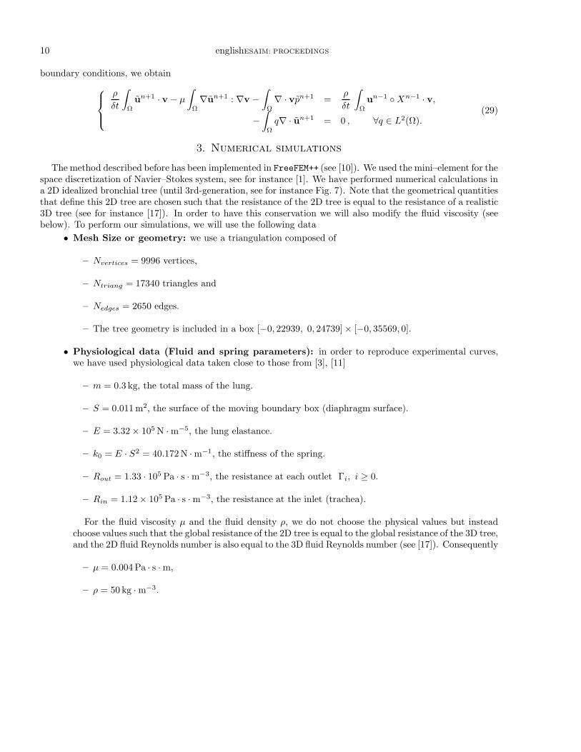
We perform calculations in a case when there is no external force. First the resistance at the inlet is equal toRin and the resistances Ri at the outlets are all taken equal to Rout. Moreover, the spring stiffness k is equalto k0. Initially, we suppose that the spring is elongated such that x(0) = 0.1 m. We plot at Fig. 3, the volumevariations V = Sx and the air flow through boundary Γ0 with respect time.

0

0.0002

0.0004

0.0006

0.0008

0.001

0.0012

0 0.5 1 1.5 2 2.5 3 0

0.0002

0.0004

0.0006

0.0008

0.001

0.0012

0.0014

0.0016

0.0018

0.002

0 0.5 1 1.5 2 2.5 3

Figure 3. Volume variation V = Sx (in m3) and air flow (in m3 · s−1) through boundary Γ0

versus time (in s).

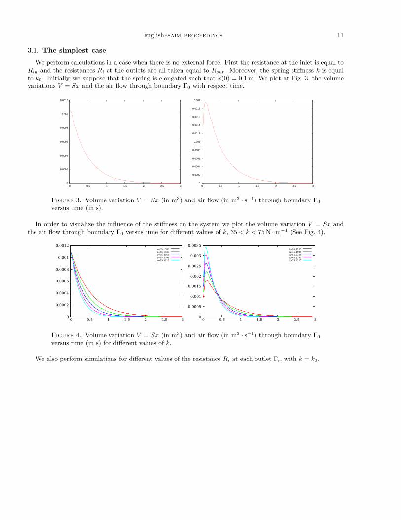
In order to visualize the influence of the stiffness on the system we plot the volume variation V = Sx andthe air flow through boundary Γ0 versus time for different values of k, 35 < k < 75 N · m−1 (See Fig. 4).


versus time (in s) for different values of k.

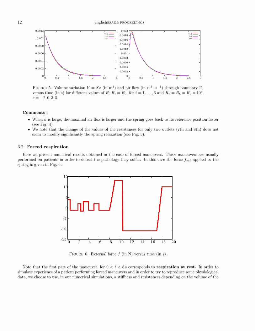
We also perform simulations for different values of the resistance Ri at each outlet Γi, with k = k0.



versus time (in s) for different values of R, Ri = R0, for i = 1, . . . , 6 and R7 = R8 = R0 × 10s,s = −2, 0, 3, 5.

Comments :

• When k is large, the maximal air flux is larger and the spring goes back to its reference position faster(see Fig. 4).

• We note that the change of the values of the resistances for only two outlets (7th and 8th) does notseem to modify significantly the spring relaxation (see Fig. 5).

3.2. Forced respiration

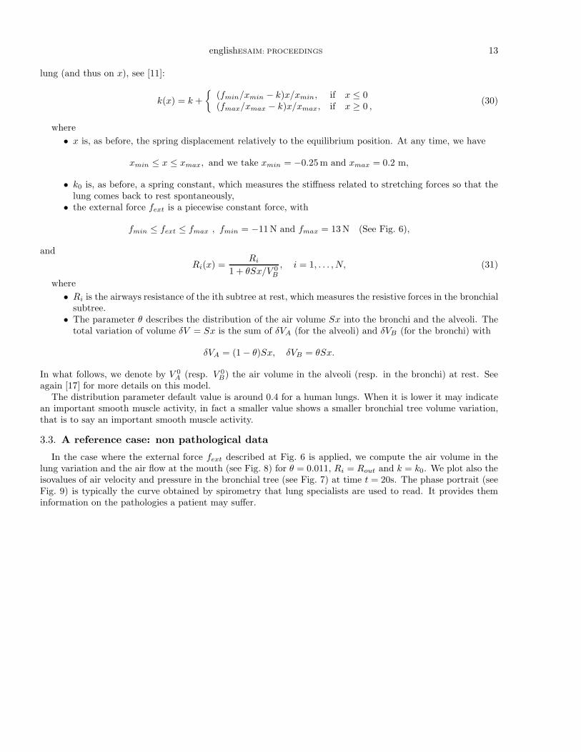
Here we present numerical results obtained in the case of forced maneuvers. These maneuvers are usuallyperformed on patients in order to detect the pathology they suffer. In this case the force fext applied to thespring is given in Fig. 6.

Figure 6. External force f (in N) versus time (in s).

Note that the first part of the maneuver, for 0 < t < 8 s corresponds to respiration at rest. In order tosimulate experience of a patient performing forced maneuvers and in order to try to reproduce some physiologicaldata, we choose to use, in our numerical simulations, a stiffness and resistances depending on the volume of the


lung (and thus on x), see [11]:

k(x) = k +

(fmin/xmin − k)x/xmin, if x ≤ 0(fmax/xmax − k)x/xmax, if x ≥ 0 ,

(30)

where

• x is, as before, the spring displacement relatively to the equilibrium position. At any time, we have

xmin ≤ x ≤ xmax, and we take xmin = −0.25 m and xmax = 0.2 m,

• k0 is, as before, a spring constant, which measures the stiffness related to stretching forces so that thelung comes back to rest spontaneously,

• the external force fext is a piecewise constant force, with

fmin ≤ fext ≤ fmax , fmin = −11 N and fmax = 13 N (See Fig. 6),

and

Ri(x) =Ri

1 + θSx/V 0B

, i = 1, . . . , N, (31)

where

• Ri is the airways resistance of the ith subtree at rest, which measures the resistive forces in the bronchialsubtree.

• The parameter θ describes the distribution of the air volume Sx into the bronchi and the alveoli. Thetotal variation of volume δV = Sx is the sum of δVA (for the alveoli) and δVB (for the bronchi) with

δVA = (1 − θ)Sx, δVB = θSx.

In what follows, we denote by V 0A (resp. V 0

B) the air volume in the alveoli (resp. in the bronchi) at rest. Seeagain [17] for more details on this model.

The distribution parameter default value is around 0.4 for a human lungs. When it is lower it may indicatean important smooth muscle activity, in fact a smaller value shows a smaller bronchial tree volume variation,that is to say an important smooth muscle activity.

3.3. A reference case: non pathological data

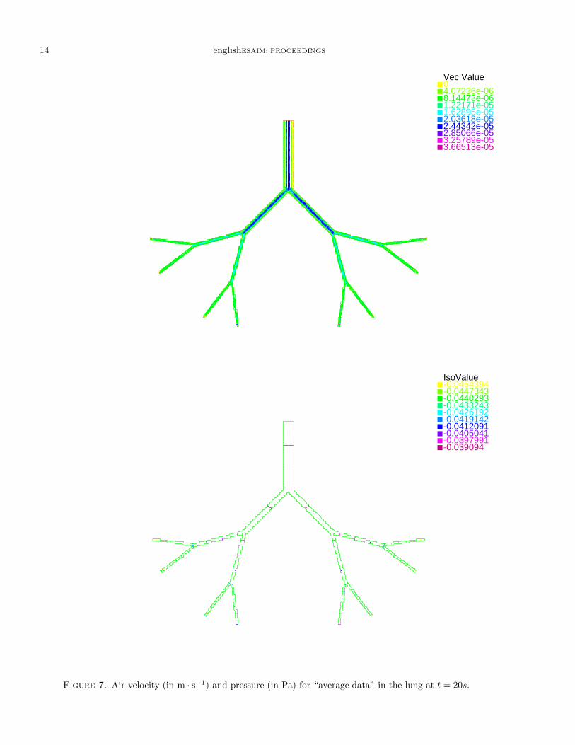
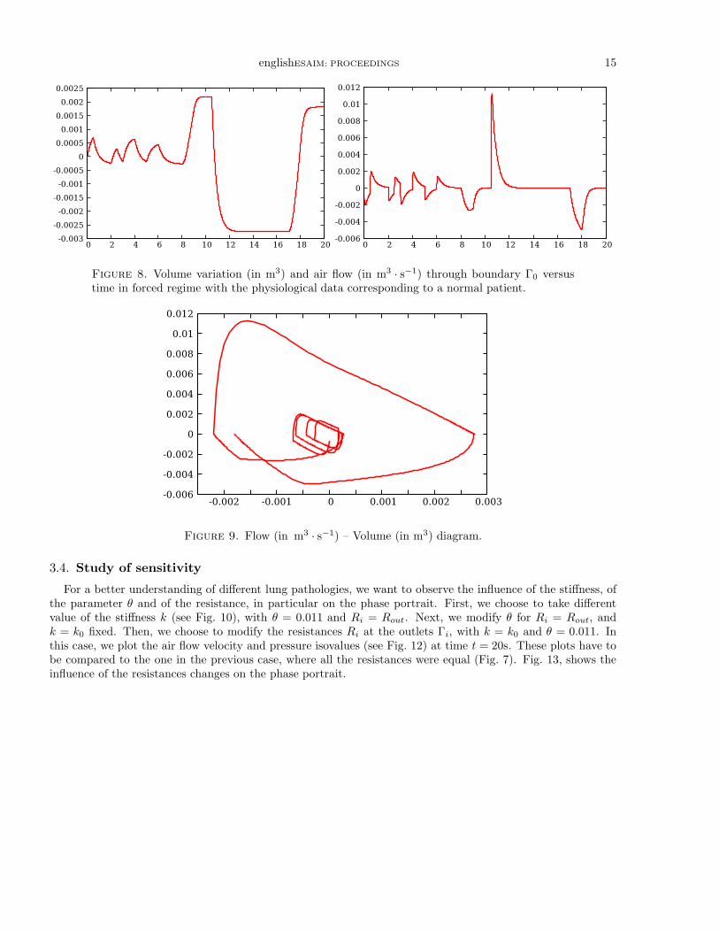
In the case where the external force fext described at Fig. 6 is applied, we compute the air volume in thelung variation and the air flow at the mouth (see Fig. 8) for θ = 0.011, Ri = Rout and k = k0. We plot also theisovalues of air velocity and pressure in the bronchial tree (see Fig. 7) at time t = 20s. The phase portrait (seeFig. 9) is typically the curve obtained by spirometry that lung specialists are used to read. It provides theminformation on the pathologies a patient may suffer.


Vec Value04.07236e-068.14473e-061.22171e-051.62895e-052.03618e-052.44342e-052.85066e-053.25789e-053.66513e-05

IsoValue-0.0454394-0.0447343-0.0440293-0.0433243-0.0426192-0.0419142-0.0412091-0.0405041-0.0397991-0.039094

Figure 7. Air velocity (in m · s−1) and pressure (in Pa) for “average data” in the lung at t = 20s.


Figure 8. Volume variation (in m3) and air flow (in m3 · s−1) through boundary Γ0 versustime in forced regime with the physiological data corresponding to a normal patient.

Figure 9. Flow (in m3 · s−1) – Volume (in m3) diagram.

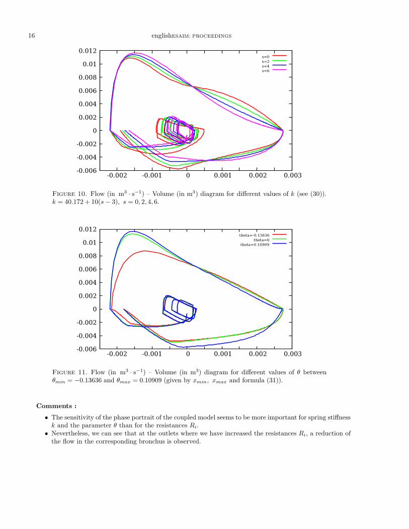
3.4. Study of sensitivity

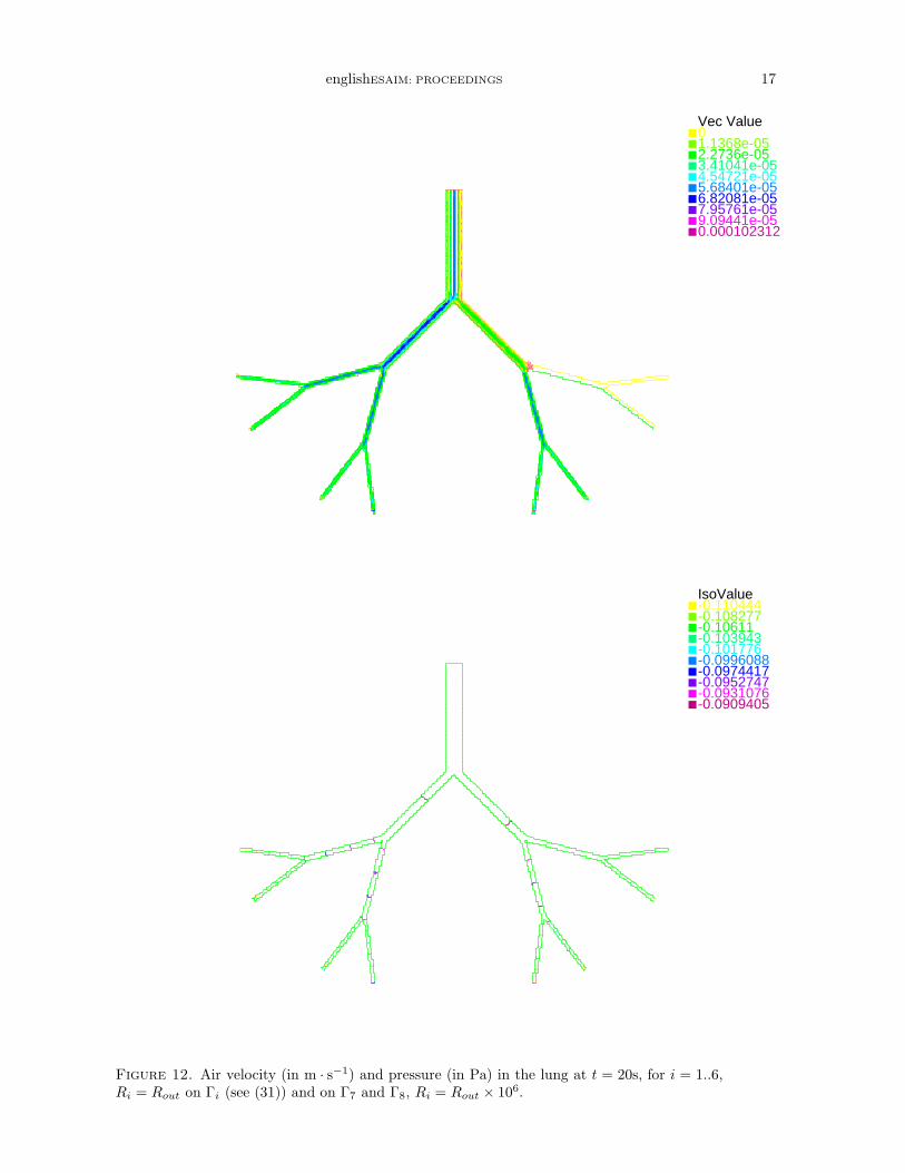
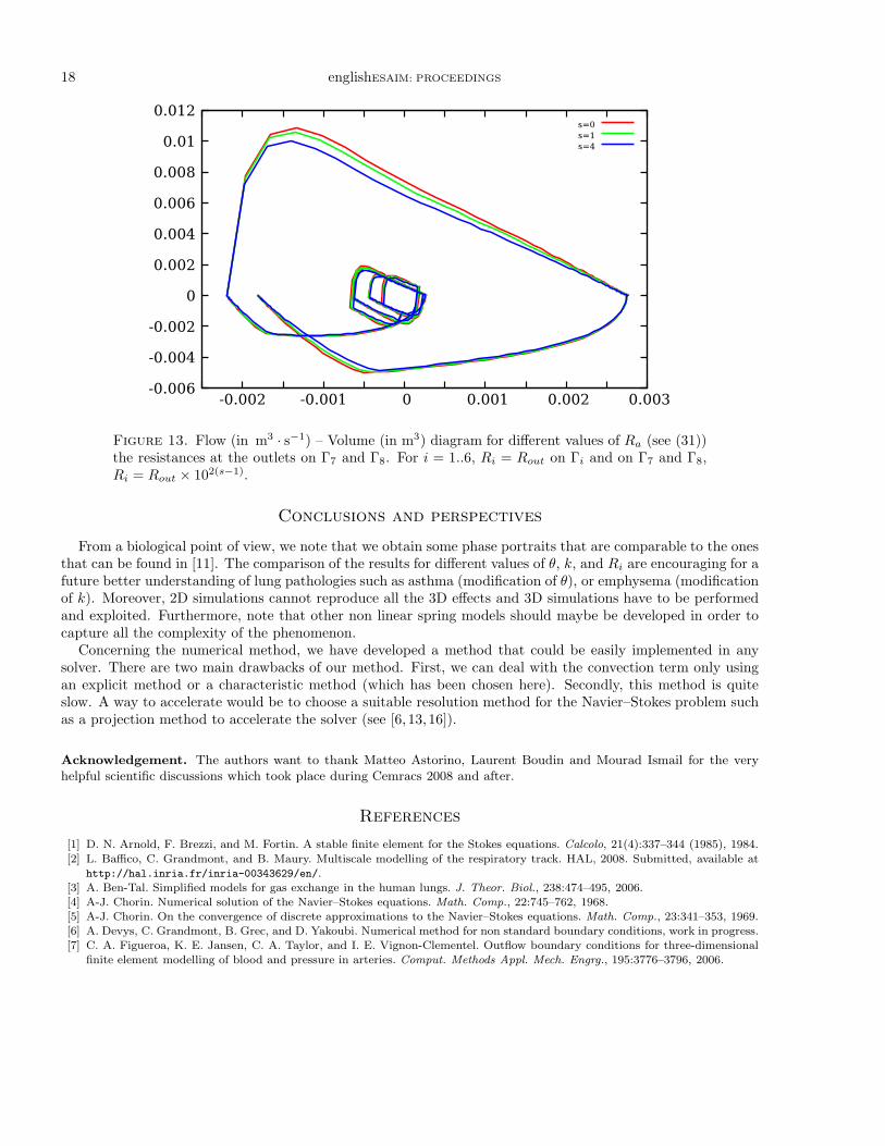
For a better understanding of different lung pathologies, we want to observe the influence of the stiffness, ofthe parameter θ and of the resistance, in particular on the phase portrait. First, we choose to take differentvalue of the stiffness k (see Fig. 10), with θ = 0.011 and Ri = Rout. Next, we modify θ for Ri = Rout, andk = k0 fixed. Then, we choose to modify the resistances Ri at the outlets Γi, with k = k0 and θ = 0.011. Inthis case, we plot the air flow velocity and pressure isovalues (see Fig. 12) at time t = 20s. These plots have tobe compared to the one in the previous case, where all the resistances were equal (Fig. 7). Fig. 13, shows theinfluence of the resistances changes on the phase portrait.


Figure 10. Flow (in m3 · s−1) – Volume (in m3) diagram for different values of k (see (30)).k = 40.172 + 10(s − 3), s = 0, 2, 4, 6.

Figure 11. Flow (in m3 · s−1) – Volume (in m3) diagram for different values of θ betweenθmin = −0.13636 and θmax = 0.10909 (given by xmin, xmax and formula (31)).

Comments :

• The sensitivity of the phase portrait of the coupled model seems to be more important for spring stiffnessk and the parameter θ than for the resistances Ri.

• Nevertheless, we can see that at the outlets where we have increased the resistances Ri, a reduction ofthe flow in the corresponding bronchus is observed.


Vec Value01.1368e-052.2736e-053.41041e-054.54721e-055.68401e-056.82081e-057.95761e-059.09441e-050.000102312

IsoValue-0.110444-0.108277-0.10611-0.103943-0.101776-0.0996088-0.0974417-0.0952747-0.0931076-0.0909405

Figure 12. Air velocity (in m · s−1) and pressure (in Pa) in the lung at t = 20s, for i = 1..6,Ri = Rout on Γi (see (31)) and on Γ7 and Γ8, Ri = Rout × 106.


Figure 13. Flow (in m3 · s−1) – Volume (in m3) diagram for different values of Ra (see (31))the resistances at the outlets on Γ7 and Γ8. For i = 1..6, Ri = Rout on Γi and on Γ7 and Γ8,Ri = Rout × 102(s−1).

Conclusions and perspectives

From a biological point of view, we note that we obtain some phase portraits that are comparable to the onesthat can be found in [11]. The comparison of the results for different values of θ, k, and Ri are encouraging for afuture better understanding of lung pathologies such as asthma (modification of θ), or emphysema (modificationof k). Moreover, 2D simulations cannot reproduce all the 3D effects and 3D simulations have to be performedand exploited. Furthermore, note that other non linear spring models should maybe be developed in order tocapture all the complexity of the phenomenon.

Concerning the numerical method, we have developed a method that could be easily implemented in anysolver. There are two main drawbacks of our method. First, we can deal with the convection term only usingan explicit method or a characteristic method (which has been chosen here). Secondly, this method is quiteslow. A way to accelerate would be to choose a suitable resolution method for the Navier–Stokes problem suchas a projection method to accelerate the solver (see [6, 13, 16]).

Acknowledgement. The authors want to thank Matteo Astorino, Laurent Boudin and Mourad Ismail for the veryhelpful scientific discussions which took place during Cemracs 2008 and after.

References

[1] D. N. Arnold, F. Brezzi, and M. Fortin. A stable finite element for the Stokes equations. Calcolo, 21(4):337–344 (1985), 1984.

[2] L. Baffico, C. Grandmont, and B. Maury. Multiscale modelling of the respiratory track. HAL, 2008. Submitted, available athttp://hal.inria.fr/inria-00343629/en/.

[3] A. Ben-Tal. Simplified models for gas exchange in the human lungs. J. Theor. Biol., 238:474–495, 2006.[4] A-J. Chorin. Numerical solution of the Navier–Stokes equations. Math. Comp., 22:745–762, 1968.[5] A-J. Chorin. On the convergence of discrete approximations to the Navier–Stokes equations. Math. Comp., 23:341–353, 1969.[6] A. Devys, C. Grandmont, B. Grec, and D. Yakoubi. Numerical method for non standard boundary conditions, work in progress.[7] C. A. Figueroa, K. E. Jansen, C. A. Taylor, and I. E. Vignon-Clementel. Outflow boundary conditions for three-dimensional

finite element modelling of blood and pressure in arteries. Comput. Methods Appl. Mech. Engrg., 195:3776–3796, 2006.


[8] C. Grandmont, Y. Maday, and B. Maury. A multiscale/multimodel approach of the respiration tree. In New trends in continuum

mechanics, volume 3 of Theta Ser. Adv. Math., pages 147–157. Theta, Bucharest, 2005.[9] C. Grandmont, B. Maury, and A. Soualah. Multiscale modelling of the respiratory track: a theoretical framework. ESAIM

Proc., 23:10–29, 2008.[10] F. Hecht, A. Le Hyaric, K. Ohtsuka, and O. Pironneau. Freefem++, finite elements software, http://www.freefem.org/ff++/.[11] S. Martin, B. Maury, T. Similowski, and C. Straus. Impact of respiratory mechanics model parameters on gas exchange

efficiency. ESAIM: PROCEEDINGS, 23, (2008) 30–47.[12] M.S. Olufsen. Structured tree outflow condition for blood flow in larger systemic arteries. Am. J. Physiol., 276:257–H268, 1999.[13] L. Quartapelle. Numerical solution of the incompressible Navier–Stokes equations. International Series of Numerical Mathe-

matics, 113, 1993.[14] A. Quarteroni, S. Ragni, and A. Veneziani. Coupling between lumped and distributed models for blood flow problems. Com-

put.Visualization Sci., 4 (2):111124, 2001.[15] A. Quarteroni and A. Veneziani. Analysis of a geometrical multiscale model based on the coupling of odes and pdes for blood

flow simulations. Multiscale Model. Simul., 1, No.2:173–195, 2003.[16] R. Rannacher. On Chorin’s projection method for the incompressible Navier–Stokes equations. Lecture Notes in Math.,

1530:167–183, 1992.[17] A. Soualah-Alilah. Modelisation mathematique et numerique du poumon humain. PhD thesis, Universite Paris-Sud–Orsay,

2007.[18] R. Temam. Navier–Stokes equations. theory and numerical analysis. Studies in Mathematics and its Applications, 2, 1977.

Documents

Numerical method for the 2D simulation of the respiration · Numerical method for the 2D simulation of the respiration ... Bertrand Maury, Driss Yakoubi. Numerical method for the