Numerical investigation of the ﬂow instabilities in centri ... · Numerical investigation of the ﬂow instabilities in centri fugal fan ... stability of the centrifugal fan

Numerical investigation of the flow instabilities in centrifugal fan

BRANIMIR MATIJA SEVICFaculty of Mechanical Engineering

and Naval ArchitectureChair of Turbomachinery

Ivana Lucica 5, 10000 ZagrebCROATIA

[email protected]

STANISLAV SVIDEREKFaculty of Mechanical Engineering

and Naval ArchitectureChair of Turbomachinery


[email protected]

TIHOMIR MIHALI CFaculty of Mechanical Engineering

and Naval ArchitectureChair of Fluid Mechanics


Abstract:It is well known in the practice that rotor blade geometry and shape of channels influence flow pattern andstability of the centrifugal fan. Practical recommendations on how to reduce the instabilities as source of energylosses and noise are based on experience and experimental approach. The research is based on the numericalapproach, instead of experimental one, for flow stabilities investigation. The calculation of flow instabilities fortwo different types of the shroud and two different number of blades are performed. The results are transferred,via FFT analysis in frequency domain, where additional conclusions about instabilities phenomena are carried out.

Key–Words:Radial fan, turbulence modeling, unsteady, DES, FFT

1 Introduction

Fluid flow in turbomachinery is highly turbulent andunsteady. Turbulent flows have been studied mostlyby means of experimental fluid dynamics research.Measuring techniques that allow sampling of flowcharacteristics in a single point have increased therange of experimental measurements. Experimentalresearch has still its limitations, especially in the fieldof rotating turbomachinery, ranging from the time re-quired to produce experimental model and its cost tothe difficult, if ever possible, measurements of flowcharacteristics in fast rotating system.

Hence, experimental methods in turbomachineryapplications are often limited to measurement of inte-gral quantities, which do not provide insight of the in-ternal flow structures. Experimental research remainsstill very important for the validation of new models.

Computational fluid dynamics is more flexibleand cost effective than experimental methods. It hasadvantage that any flow quantity may be sampled atany point in the field. Instantaneous field values canbe obtained for the whole domain, thus providing fullinsight of the flow characteristics and intricate flowstructures. Major drawback of the numerical simu-lations is their inability to guarantee accuracy underall conditions. Strictly speaking, results of numericalsimulations must be validated by experimental data.

Still, even without experimental support, numer-ical simulations can be valuable in design analysis.They provide useful insight of flow characteristicsand comparison between different geometry configu-

rations.In this study, unsteady turbulent fluid flow in a

radial fan impeller is investigated by use of computa-tional fluid dynamics methods. Two geometry config-urations are compared at several flow rates. Resultsinclude frequency analysis of the flow unsteadyness.

2 Turbulence Modeling

First approach to the practical numerical simulationof turbulent flow in a turbomachine could be, the leastexpensive and fastest, solving of steady Reynolds Av-eraged Navier-Stokes (RANS) equations in rotationalframe of reference, coupled with appropriate k-ǫ tur-bulence model with wall functions.

In RANS, flow variables are split between onetime-averaged mean part and one turbulent (fluctuat-ing) part. The latter is modelled with a turbulencemodel such as k-ǫ, Spalart-Allmaras or ReynoldsStress Model.

The RANS results show acceptable agreementwith analytically predicted as well as experimentallymeasured integral quantities such as flow rate, headand efficiency in the vicinity of the design workingpoint.

However, in off-design working conditions, whenunsteadiness and flow separation become significant,this approach gives less acceptable results. SteadyRANS equations are designed to smear out not onlythe high frequency unsteady turbulent fluctuations butalso the low frequency main flow unsteadiness. The

Proceedings of the 4th WSEAS International Conference on Fluid Mechanics and Aerodynamics, Elounda, Greece, August 21-23, 2006 (pp282-288)

wall functions which assume attached boundary layerflow do not cope well with flow separation.

Another approach to modeling of turbulent flowsis Large Eddy Simulation (LES). Idea is to computethe contributions of the large, energy-carrying struc-tures to momentum and energy transfer and to modelthe effects of the small structures, which are not re-solved by the numerical scheme. In LES only small,isotropic turbulent scales are modeled. Large scalefluctuations, which strongly depend on the geometryand boundary conditions are fully resolved.

LES is based on a spatial filtering, which decom-poses any flow variable into a filtered (large-scale,resolved) part and into a sub-filter (unresolved) part.In finite volume method, a volume filter defined bycomputational grid is used to form governing equa-tions. Volume filter filters out fluctuations in spacewith scales smaller then grid (cell) size. Furthermore,filtering is implicit which means that equations arediscretized and filtered over the same control volume.Turbulent scales which cannot be resolved by the gridare then modeled by subgrid scale model.

LES is less demanding on computational re-sources than DNS since not all scales need to be re-solved, but considerably more demanding than steadystate RANS due to higher resolution requirements andits unsteady nature. Furthermore, presence of solidwalls in the flow domain requires very fine grid whichmakes LES impractical in modelling of wall boundedflows at higher Reynolds numbers.

In order to avoid requirement of very fine meshnear the wall and extend LES to high Reynoldsnumber flows, several methods have been developed.These include Unsteady Reynolds Averaged Navier-Stokes (URANS), Detached Eddy Simulation (DES)and Hybrid LES-RANS.

URANS equations are usual RANS equations butwith the transient term retained. However, URANSis not a simple transposition of RANS (steady-stateflows in statistical equilibrium) in unsteady flows.Turbulence models and discretization schemes used inURANS are adapted to unsteadiness and detachmentof flow. URANS models are able to accurately pre-dict flows under adverse pressure gradients, includingflows with small separation bubbles.

DES is a mix of LES and RANS. Domi-nant eddies in massively separated flows are highlygeometry-specific and have not much in common withthe standard eddies of the thin shear flows RANSmodels are designed to model. The general idea ofDES is to model attached boundary layer vertices inRANS mode and capture the outer detached eddieswith LES. Small, subgrid scale vertices in LES regionare also modelled, but they have much less influencethen the boundary layer vertices. The name Detached

Eddy Simulation owes its name to the fact that onlydetached eddies are simulated while other are mod-elled.

2.1 Detached eddy simulationDES is an approach whereby RANS turbulence mod-eling and mesh spacing is used in the boundary layer,while LES is employed in the core and separated re-gions of the flow. Thin shear layer turbulence modelcontrols the solution in the RANS region. In the LESregion, turbulence model has little effect since thelarger, energy carrying vortices are resolved. Throughthe use of the near-wall RANS model, DES reducecomputational cost over conventional LES by remov-ing wall parallel resolution requirements. Typically,wall normal resolution requirements remain still highdue to the required spacing in wall units (y+) of theorder of one, similar to the low-Reynolds numberRANS turbulence models.

DES model proposed by [8] solves set of URANSequations:

∂Uj

∂xj

= 0 (1)

∂Ui

∂t+

∂(UiUj)

∂xj

= −

1

ρ

∂P

∂xi

+ν∂2Ui

∂xj∂xj

−

∂u′′

i u′′

j

∂xj

(2)

where the Spalart-Allmaras turbulence model [7] isused to compute Reynolds-stress tensor (3):

−

∂u′′

i u′′

j

∂xj

= −

∂

∂xj

(UiUj − UiUj) =1

ρ

∂

∂xj

τRij (3)

The standard Spalart-Allmaras model uses the dis-tance to the closest wall as the definition for the lengthscaled, which plays a major role in determining thelevel of production and destruction of turbulent vis-cosity. The DES model replacesd everywhere with anew length scaled, defined as:

d = min(d,Cdes∆) (4)

where the grid spacing,∆, is based on the largestcell edge length in thex, y, or z direction, ∆ =max(∆x,∆y,∆z). The empirical constantCdes hasa value of 0.65. In the boundary layerd < Cdes∆ andmodel operates in RANS mode. Outside of the bound-ary layerd > Cdes∆ model operates as subgrid-scaleLES model.

In standard DES, RANS portion of the simula-tion is strongly grid dependant. RANS requires thatgrid spacing in both wall parallel directions be largerthen the boundary layer thickness at that wall location.This is a restrictive lower limit for the grid resolution,which may easily be violated. Further grid refinement


φ10

00φ56

0

110

φ10

00φ56

0

65

110

φ50

0

φ50

0

Figure 1: Two impeller shapes, flat and cone shapedshroud, with major dimensions

below this limit, which is equivalent to the placingof the LES/RANS interface deeper into the boundarylayer, can result in non-physical grid induced separa-tion.

3 Model Details

An inlet/exit diameter ratioD1/D2 = 0.56 is upperallowable limit for radial impellers with constant im-peller width (flat shroud) [1]. For higher values ofD1/D2 ratio, a reduction of impeller width is recom-mended in order to keep diffusivity ratio of the bladechannel under control. An impeller with inlet/exit di-ameter ratioD1/D2 = of exactly 0.56 is chosen tocompare effect of the reduced impeller width on flowcharacteristics of the impeller.

Thus, two geometrically different configurations(Figure 1) are modeled, one with flat shroud and theother with conical shroud.

Basic geometry parameters are common to bothconsidered impellers: diameter of the suction tubeDs = 500 mm, impeller inlet diameterD1 = 560mm, impeller inlet widthb1 = 110 mm, impeller exitdiameterD2 = 1000 mm. Blades are formed as singlecircular arc with 732.2 mm radius. Inlet angleβ1 =30◦, outlet blade angleβ2 = 44◦.

Because of rotational periodicity of the impelleronly a single blade channel needs to be modeled. Pe-riodic boundaries form an angle which is equal to2πdivided by number of blades.

In order to allow simulation of only one portion ofthe domain, instead into volute, impellers dischargeinto a vaneless diffuser ofR3 = 800 mm outer ra-dius. Width of diffuser is matched to the exit impellerwidth. On the upper end of the diffuser, there is an

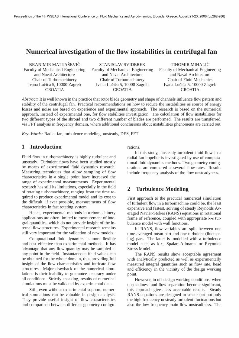
periodic

blade (wall)

periodic

wall

outlet vent

pressure inlet

Figure 2: Computational domain and boundary condi-tions. Single cyclic symmetric sector which containsone blade passage is modelled

outlet formed as axial 12.5 mm wide annulus on theboth sides. Such outlet is chosen in order to mini-mize outlet boundary impact on upstream flow, to pre-vent possible backflow condition on outlet and to se-cure the same outlet cross-section area for any diffuserwidth (Figure 2).

Computational domain upstream of the impelleris extended to form a suction pipe which is widenedat the inlet, to minimize effect of inlet boundary onthe flow inside impeller. Inlet is formed as a sphericalsurface.

Rotational moving of the impeller is numericallytaken into account by usage of multiple referenceframes. Inlet section of the suction tube as well as theoutlet section of the diffuser are calculated in station-ary reference frames. Blades as well as other movingwalls (backplate and shroud) are fixed to the movingreference frame. This approach seems to be reason-able since there is no stationary blades before or afterthe impeller. In fact, whole domain could be repre-sented by a single rotating reference frame.

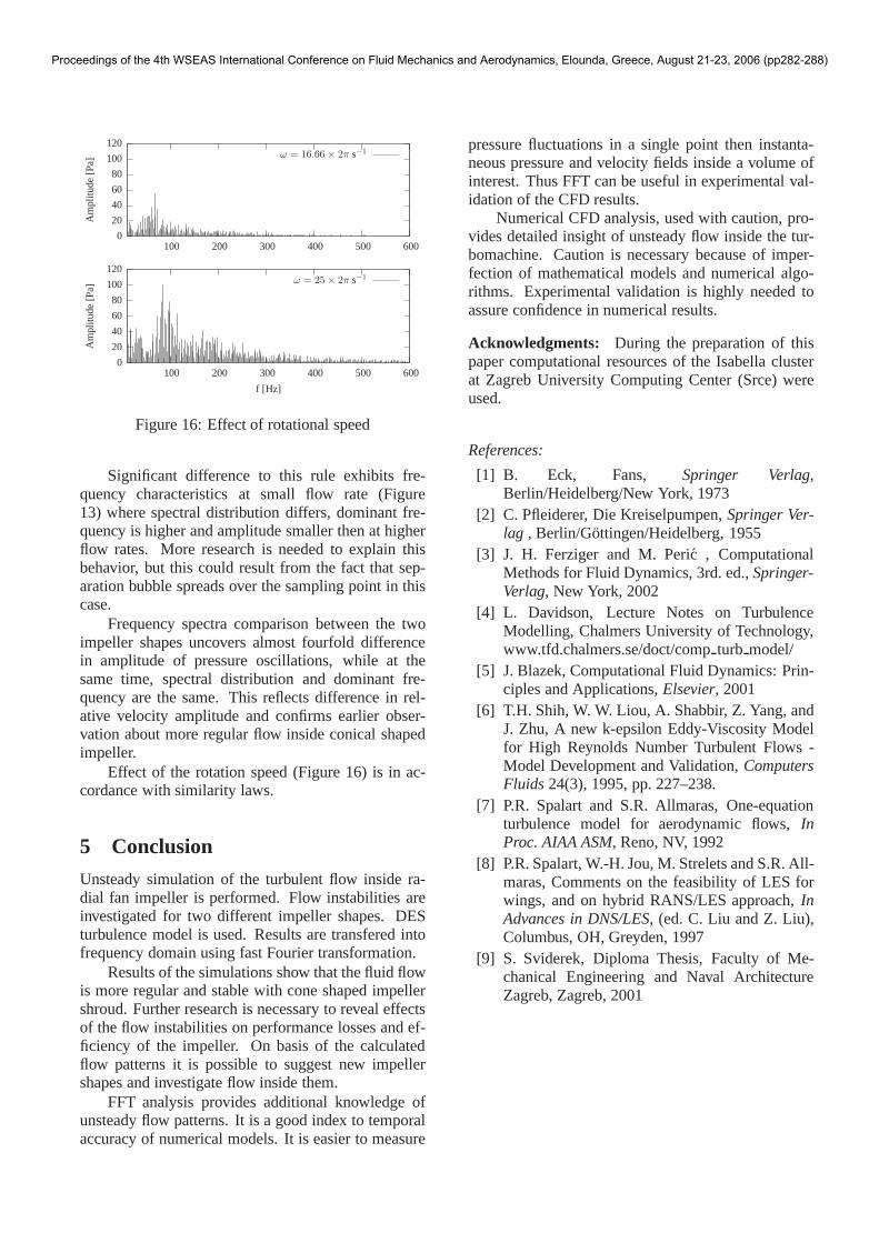
Angular velocity of the impeller was set atω =25 × 2π s−1, except in one comparison case where itwas set at16.66 × 2π s−1.

A constant total pressure and normal velocity di-rection are prescribed on inlet. On outlet, static pres-sure is given as a function of normal velocity com-ponent and prescribed nondimensional pressure dropcoefficient in the form:

pout = kL

1

2ρv2

Near design flow rate was achieved with the pres-sure drop coefficient value ofkL = 10. Values of 25and 200 were used to simulate flow regimes at smallerflow rates. This boundary condition mimic behav-ior of throttling valve and approximates natural outlet


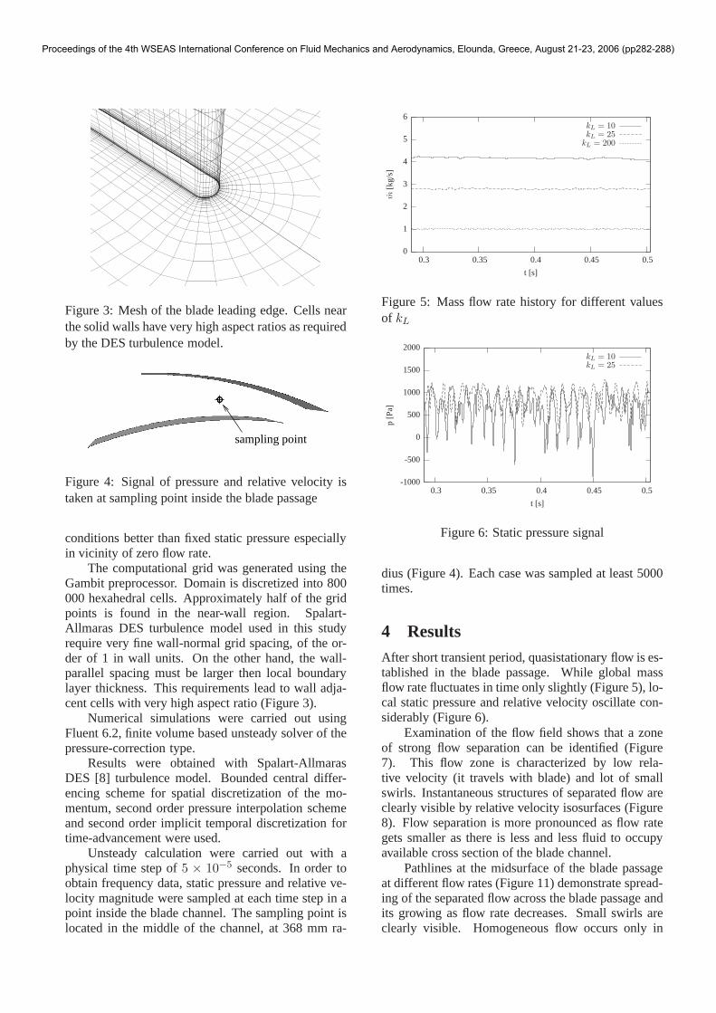
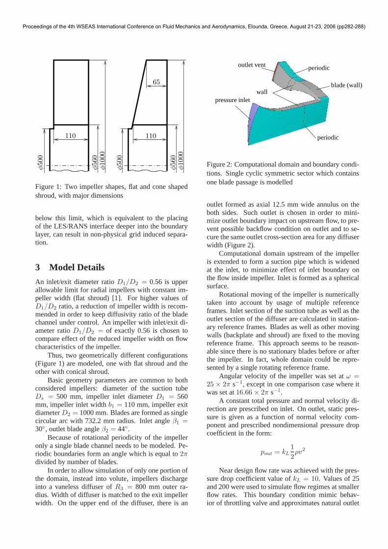
Figure 3: Mesh of the blade leading edge. Cells nearthe solid walls have very high aspect ratios as requiredby the DES turbulence model.

sampling point

Figure 4: Signal of pressure and relative velocity istaken at sampling point inside the blade passage

conditions better than fixed static pressure especiallyin vicinity of zero flow rate.

The computational grid was generated using theGambit preprocessor. Domain is discretized into 800000 hexahedral cells. Approximately half of the gridpoints is found in the near-wall region. Spalart-Allmaras DES turbulence model used in this studyrequire very fine wall-normal grid spacing, of the or-der of 1 in wall units. On the other hand, the wall-parallel spacing must be larger then local boundarylayer thickness. This requirements lead to wall adja-cent cells with very high aspect ratio (Figure 3).

Numerical simulations were carried out usingFluent 6.2, finite volume based unsteady solver of thepressure-correction type.

Results were obtained with Spalart-AllmarasDES [8] turbulence model. Bounded central differ-encing scheme for spatial discretization of the mo-mentum, second order pressure interpolation schemeand second order implicit temporal discretization fortime-advancement were used.

Unsteady calculation were carried out with aphysical time step of5 × 10−5 seconds. In order toobtain frequency data, static pressure and relative ve-locity magnitude were sampled at each time step in apoint inside the blade channel. The sampling point islocated in the middle of the channel, at 368 mm ra-

0

1

2

3

4

5

6

0.3 0.35 0.4 0.45 0.5

m[k

g/s]

t [s]

kL = 10kL = 25

kL = 200

Figure 5: Mass flow rate history for different valuesof kL

-1000

-500

0

500

1000

1500

2000

0.3 0.35 0.4 0.45 0.5

p[P

a]

t [s]

kL = 10kL = 25

Figure 6: Static pressure signal

dius (Figure 4). Each case was sampled at least 5000times.

4 ResultsAfter short transient period, quasistationary flow is es-tablished in the blade passage. While global massflow rate fluctuates in time only slightly (Figure 5), lo-cal static pressure and relative velocity oscillate con-siderably (Figure 6).

Examination of the flow field shows that a zoneof strong flow separation can be identified (Figure7). This flow zone is characterized by low rela-tive velocity (it travels with blade) and lot of smallswirls. Instantaneous structures of separated flow areclearly visible by relative velocity isosurfaces (Figure8). Flow separation is more pronounced as flow rategets smaller as there is less and less fluid to occupyavailable cross section of the blade channel.

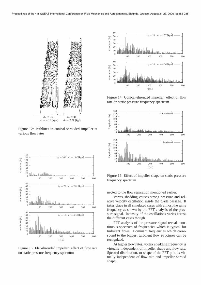
Pathlines at the midsurface of the blade passageat different flow rates (Figure 11) demonstrate spread-ing of the separated flow across the blade passage andits growing as flow rate decreases. Small swirls areclearly visible. Homogeneous flow occurs only in


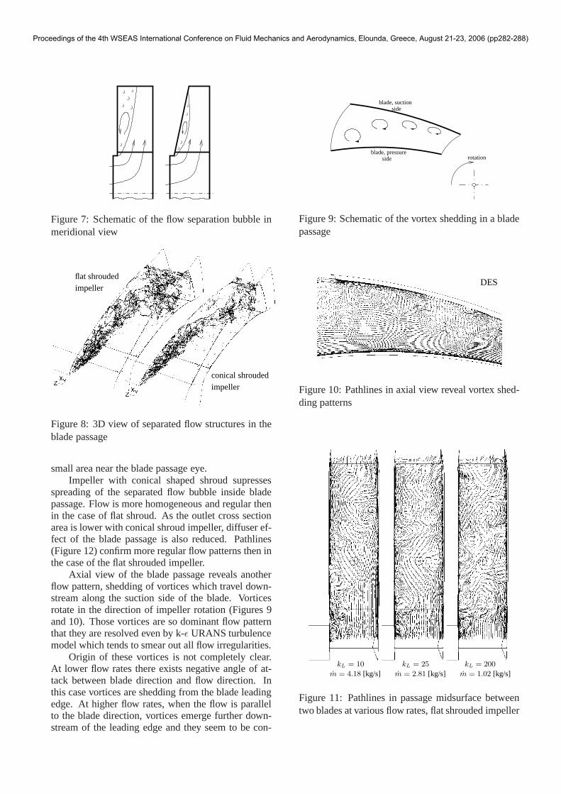
Figure 7: Schematic of the flow separation bubble inmeridional view

impeller

impellerconical shrouded

flat shrouded

Figure 8: 3D view of separated flow structures in theblade passage

small area near the blade passage eye.Impeller with conical shaped shroud supresses

spreading of the separated flow bubble inside bladepassage. Flow is more homogeneous and regular thenin the case of flat shroud. As the outlet cross sectionarea is lower with conical shroud impeller, diffuser ef-fect of the blade passage is also reduced. Pathlines(Figure 12) confirm more regular flow patterns then inthe case of the flat shrouded impeller.

Axial view of the blade passage reveals anotherflow pattern, shedding of vortices which travel down-stream along the suction side of the blade. Vorticesrotate in the direction of impeller rotation (Figures 9and 10). Those vortices are so dominant flow patternthat they are resolved even by k-ǫ URANS turbulencemodel which tends to smear out all flow irregularities.

Origin of these vortices is not completely clear.At lower flow rates there exists negative angle of at-tack between blade direction and flow direction. Inthis case vortices are shedding from the blade leadingedge. At higher flow rates, when the flow is parallelto the blade direction, vortices emerge further down-stream of the leading edge and they seem to be con-

blade, pressureside

sideblade, suction

rotation

Figure 9: Schematic of the vortex shedding in a bladepassage

DES

Figure 10: Pathlines in axial view reveal vortex shed-ding patterns

kL = 10 kL = 25 kL = 200

m = 2.81 [kg/s]m = 4.18 [kg/s] m = 1.02 [kg/s]

Figure 11: Pathlines in passage midsurface betweentwo blades at various flow rates, flat shrouded impeller


kL = 25kL = 10

m = 4.16 [kg/s] m = 2.77 [kg/s]

Figure 12: Pathlines in conical-shrouded impeller atvarious flow rates

020406080

100120140160

100 200 300 400 500 600

Am

plitu

de[P

a]

kL = 200, m = 1.02 [kg/s]

020406080

100120140160

100 200 300 400 500 600

Am

plitu

de[P

a]

kL = 25, m = 2.81 [kg/s]

020406080

100120140160

100 200 300 400 500 600

Am

plitu

de[P

a]

f [Hz]

kL = 10, m = 4.18 [kg/s]

Figure 13: Flat-shrouded impeller: effect of flow rateon static pressure frequency spectrum

0

10

20

30

40

50

60

100 200 300 400 500 600

Am

plitu

de[P

a]

kL = 25, m = 2.77 [kg/s]

0

10

20

30

40

50

60

100 200 300 400 500 600

Am

plitu

de[P

a]

f [Hz]

kL = 10, m = 4.16 [kg/s]

Figure 14: Conical-shrouded impeller: effect of flowrate on static pressure frequency spectrum

020406080

100120140160

100 200 300 400 500 600

Am

plitu

de[P

a]

conical shroud

020406080

100120140160

100 200 300 400 500 600

Am

plitu

de[P

a]

f [Hz]

flat shroud

Figure 15: Effect of impeller shape on static pressurefrequency spectrum

nected to the flow separation mentioned earlier.Vortex shedding causes strong pressure and rel-

ative velocity oscillation inside the blade passage. Ittakes place in all simulated cases with almost the samefrequency as shown by the FFT analysis of the pres-sure signal. Intensity of the oscillations varies acrossthe different cases though.

FFT analysis of the pressure signal reveals con-tinuous spectrum of frequencies which is typical forturbulent flows. Dominant frequencies which corre-spond to the biggest turbulent flow structures can berecognized.

At higher flow rates, vortex shedding frequency isvirtually independent of impeller shape and flow rate.Spectral distribution, or shape of the FFT plot, is vir-tually independent of flow rate and impeller shroudshape.


0

20

40

60

80

100

120

100 200 300 400 500 600

Am

plitu

de[P

a]

ω = 16.66 × 2π s−1

0

20

40

60

80

100

120

100 200 300 400 500 600

Am

plitu

de[P

a]

f [Hz]

ω = 25 × 2π s−1

Figure 16: Effect of rotational speed

Significant difference to this rule exhibits fre-quency characteristics at small flow rate (Figure13) where spectral distribution differs, dominant fre-quency is higher and amplitude smaller then at higherflow rates. More research is needed to explain thisbehavior, but this could result from the fact that sep-aration bubble spreads over the sampling point in thiscase.

Frequency spectra comparison between the twoimpeller shapes uncovers almost fourfold differencein amplitude of pressure oscillations, while at thesame time, spectral distribution and dominant fre-quency are the same. This reflects difference in rel-ative velocity amplitude and confirms earlier obser-vation about more regular flow inside conical shapedimpeller.

Effect of the rotation speed (Figure 16) is in ac-cordance with similarity laws.

5 Conclusion

Unsteady simulation of the turbulent flow inside ra-dial fan impeller is performed. Flow instabilities areinvestigated for two different impeller shapes. DESturbulence model is used. Results are transfered intofrequency domain using fast Fourier transformation.

Results of the simulations show that the fluid flowis more regular and stable with cone shaped impellershroud. Further research is necessary to reveal effectsof the flow instabilities on performance losses and ef-ficiency of the impeller. On basis of the calculatedflow patterns it is possible to suggest new impellershapes and investigate flow inside them.

FFT analysis provides additional knowledge ofunsteady flow patterns. It is a good index to temporalaccuracy of numerical models. It is easier to measure

pressure fluctuations in a single point then instanta-neous pressure and velocity fields inside a volume ofinterest. Thus FFT can be useful in experimental val-idation of the CFD results.

Numerical CFD analysis, used with caution, pro-vides detailed insight of unsteady flow inside the tur-bomachine. Caution is necessary because of imper-fection of mathematical models and numerical algo-rithms. Experimental validation is highly needed toassure confidence in numerical results.

Acknowledgments: During the preparation of thispaper computational resources of the Isabella clusterat Zagreb University Computing Center (Srce) wereused.

References:

[1] B. Eck, Fans, Springer Verlag,Berlin/Heidelberg/New York, 1973

[2] C. Pfleiderer, Die Kreiselpumpen,Springer Ver-lag , Berlin/Gottingen/Heidelberg, 1955

[3] J. H. Ferziger and M. Peric , ComputationalMethods for Fluid Dynamics, 3rd. ed.,Springer-Verlag, New York, 2002

[4] L. Davidson, Lecture Notes on TurbulenceModelling, Chalmers University of Technology,www.tfd.chalmers.se/doct/compturb model/

[5] J. Blazek, Computational Fluid Dynamics: Prin-ciples and Applications,Elsevier, 2001

[6] T.H. Shih, W. W. Liou, A. Shabbir, Z. Yang, andJ. Zhu, A new k-epsilon Eddy-Viscosity Modelfor High Reynolds Number Turbulent Flows -Model Development and Validation,ComputersFluids 24(3), 1995, pp. 227–238.

[7] P.R. Spalart and S.R. Allmaras, One-equationturbulence model for aerodynamic flows,InProc. AIAA ASM, Reno, NV, 1992

[8] P.R. Spalart, W.-H. Jou, M. Strelets and S.R. All-maras, Comments on the feasibility of LES forwings, and on hybrid RANS/LES approach,InAdvances in DNS/LES, (ed. C. Liu and Z. Liu),Columbus, OH, Greyden, 1997

[9] S. Sviderek, Diploma Thesis, Faculty of Me-chanical Engineering and Naval ArchitectureZagreb, Zagreb, 2001


Documents

Numerical investigation of the ﬂow instabilities in centri ... · Numerical investigation of the ﬂow instabilities in centri fugal fan ... stability of the centrifugal fan