Inter J Nav Archit Oc Engng (2011) 3:122~125

http://dx.doi.org/10.2478/IJNAOE-2013-0054

ⓒSNAK, 2011

Numerical investigation of floating breakwater movement using SPH method

A. Najafi-Jilani1 and A. Rezaie-Mazyak

2

1 Civil Engineering, Islamic Azad University, Islamshahr Branch, Iran

2 Civil Engineering, Tarbiat Modares University, Tehran, Iran

ABSTRACT: In this work, the movement pattern of a floating breakwater is numerically analyzed using Smoothed Particle Hydrodynamic (SPH) method as a Lagrangian scheme. At the seaside, the regular incident waves with varying height and period were considered as the dynamic free surface boundary conditions. The smooth and impermeable beach slope was defined as the bottom boundary condition. The effects of various boundary conditions such as incident wave characteristics, beach slope, and water depth on the movement of the floating body were studied. The numerical results are in good agreement with the available experimental data in the literature The results of the movement of the floating body were used to determine the transmitted wave height at the corresponding boundary conditions

KEY WORDS: Floating Breakwater; Smoothed Particle Hydrodynamics(SPH); Paddle Wavemaker; Regular Waves

INTRODUCTION

Floating breakwater is generally used to maintain

tranquility in port. It is also used frequently in marine

works, military operations, fishery activities, recreational

ports etc. Navigation and harboring of ships in many ports

are significantly affected by influx of waves. Hence, floating

breakwater is necessary to reduce wave heights in a specific

location to minimize the impact of the waves, thereby

providing safe environment for ships and increasing overall

efficiency.

The first record of using floating structure as a

breakwater dates back to the early19th

century. In 1811,

General Bentham, the Civil Architect and Principal

Surveyor of the Royal Navy of Great Britain, proposed a

breakwater model for the British fleet at Plymouth. The

breakwater consisted of triangular sections of floating wood

frames moored with iron chains. Although, its cost was

about one-tenth the finally adopted rubble and granite

mound structure, the idea was rejected due to concerns

about its effectiveness during severe storms (Ozeren, 2009;

Tu et al. 2008).

Simulation of laboratory conditions with numerical models

offers means to study and understand the physical model more

effectively. Several types of numerical models and software

development platforms are available for simulation of waves.

Paddle wave maker with CFD is one such simulation tool,

which uses a discrete approach based on finite volume (Panahi

et al. 2010). In this paper, two-dimensional simulations were

made using the Paddle Wave maker with Smoothed Particle

Hydrodynamic (SPH) method.

SPH method is the oldest mesh less particle method,

developed independently by Monaghan (1994) to simulate

the asymmetry problems in astrophysics and used to predict

the motion of separated particles with respect to time. SPH

method using Lagrangian technique has been used

successfully for simulation of free surface hydrodynamics.

As examples, it has been used for surface flows including

waves in the smooth beaches, plunging wave breaker and

simulation of dam failure. It has also shown high potential for

simulation of a wide range of numerical models such as

coastal waves, wave form of landslide, wave impact on

structures and dams etc.

The broad objective of the present study is to simulate the

interactions of waves of varying height and period with the

floating breakwater structure using the SPH method.

MATHEMATICAL FORMULATION

The general formulation of any function can be

represented by an integral equation of the following

form(Dalrymple, 2007):

( ) ( ') ( - ') '

f x f x x x dx (1)

where, f is the function of the position vector x, Ω is the

integral volume which x encompasses, and δ(x-x’) is the

Dirac delta function, which is defined as follows:

Corresponding author: A. Najafi-Jilani e-mail: a.jilani@iiau.ac.ir

Copyright © 2011 Society of Naval Architects of Korea. Production and hosting by ELSEVIER B.V. This is an open access article under the CC BY-NC 3.0 license

( http://creativecommons.org/licenses/by-nc/3.0/ ).

Inter J Nav Archit Oc Engng (2011) 3:122~125 123

1, '( ')

0, '

x xx x

x x (2)

If f(x) in domain Ω on the right side of equation (1) is

defined, the exact value of the function f(x) can be obtained.

By substituting the Dirac delta function with the smoothing

kernel function, smoothing function, or in short kernel W (x-

x’, h), f(x) takes the following form:

( ) ( ')W( - ', ) '

f x f x x x h dx (3)

where, h represents the smoothing length or influence

length of W function, and specifies the range of integral. The

kernel function becomes zero outside this area.

In the SPH method, the continuous fluid environment is

separated into a set of discrete elements (referred to as

particles). The physical quantity of any particle can be

obtained by summing the relevant properties of all the

particles which lie within the range of integral the kernel

approximation function. The integral form can be converted

to series form if dx' in particle space is converted to finite

particle volume (ΔVj). The particle mass (mj) can then be

estimated by the following equation:.

j j j

m V (4)

where, ρj is the density of particle j. The discrete form of

the equation can be represented by:

u 1( ) W

j

i j i ij

i jj

mdp g

dt (5)

where, N is the number of particles. The final form of the

equation can be represented by:

1

( ) ( ') W

N

j

ij

jj

mf x f x (6)

The interpolation of smoothing kernel function plays a

key role in SPH method. Generally, kernel of three point is

important:

estimation of pattern and interpolation of field function,

setting dimensions of field effect,

accurate and consistent interpolation in discrete state

(approximate kernel).

2 3

3

3 31 0 1

2 4

1W( , ) (2 ) 1 2

4

0 2

D

q q q

r h q q

q

(7)

In the present study, cubic kernel function of the

following form has been used for the simulation (7).

Various parameters in the above equation are defined as

follows:

jr x x , rqh

, 2

10

7D h

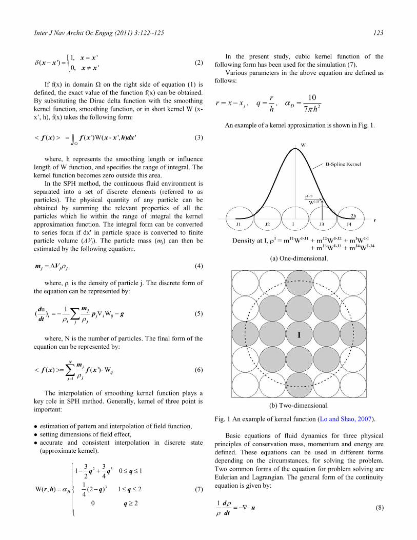
An example of a kernel approximation is shown in Fig. 1.

(a) One-dimensional.

(b) Two-dimensional.

Fig. 1 An example of kernel function (Lo and Shao, 2007).

Basic equations of fluid dynamics for three physical

principles of conservation mass, momentum and energy are

defined. These equations can be used in different forms

depending on the circumstances, for solving the problem.

Two common forms of the equation for problem solving are

Eulerian and Lagrangian. The general form of the continuity

equation is given by:

1

du

dt (8)

124 Inter J Nav Archit Oc Engng (2011) 3:122~125

where, u is the speed and ρ is the fluid density. Equation

(8) in series form is expressed by equation (9) as follows:

1( ) u W

j

i j ij

jj

md

dt (9)

where, )( jiij xxWW . Gradient kernel for second

particle (j) is equal the negative gradient kernel for the first

particle (i). The Lagrangian form of momentum equation is

expressed as:

2

0 0

u 1

cB

dp g

dt

(10)

where, g is the acceleration due to gravity, and p is the

pressure.

Momentum equation in the form of the SPH method is

shown in equation (11).

u 1( ) W

j

i j i ij

i jj

mdp g

dt (11)

Regardless of viscosity, instability develops in some

phenomena modeling with SPH method. Boiling is one of

these forms of instability which make the particles to move

irregularly(Monaghan, 1999). In the present study, since

laminar viscosity is considered, the momentum equation

changes to the following form:

2

0

1

duP g u

dt (12)

In the above equation, νo is the kinematics viscosity in

laminar flow and its value is 10-6

m2.s

-1. The viscosity term in

the SPH method is written as follows (Dalrymple, 2007).

02

0 2

4

( )

ij

b

i j

r Wu m u

r (13)

NUMERICAL MODELING

The fluid in the SPH formalism is assumed as weakly

compressible. This facilitates the use of an equation of state to

determine fluid pressure, which can be solved much faster than

the Poisson s equation. However, the compressibility is

adjusted to lower the speed of sound so that the time step in the

model (using a Courant condition for the speed of sound) is

reasonable. Another limitation on the compressibility is

imposed by the requirement that sound speed should be about

ten times faster than the maximum fluid velocity, thereby

keeping density variations to less than 1%.

Following relationship between pressure and density is

assumed to follow the expression (Monaghan and Kos, 1999).

[( ) 1]

s

s

p B (14)

where, g = 7, B= 2

0 0

c, o = reference density (1000 kg

m-3),and 00 0( ) ( / ) c c P the speed of sound at

the reference density.

BOUNDARY CONDITIONS

Unlike mesh-based methods such as finite element and

finite difference, the boundary conditions for mesh less

modeling methods such as SPH isn’t very straightforward.

SPH method boundary conditions suffer from lack of

consistency in the continuous approximation requiring

special measures to simulate these areas. For modeling, a

fixed set of virtual particles is used on the fluid interface

and solid surface (Monaghan and Kos, 1999). The function

of these virtual particles is to create a force in the opposite

direction to particles moving close to each other to prevent

water particles from crossing a solid boundary. The

particles constituting the boundary exert central forces,

analogous to intermolecular forces on the fluid particles.

Free surface is detected by computing the density of

particles. Weighted interpolation employed in SPH

method indicated a decreased density outside the free

surface, suggesting absence of particles . If the density is

less than 1% of its value for the internal fluid particles, the

particle component is considered as free surface. It is

required to compare the laboratory experimental data with

the numerical simulation results to verify the model. As

the simulated Paddle Wave maker only has the ability to

make regular waves, it can be used for generating waves

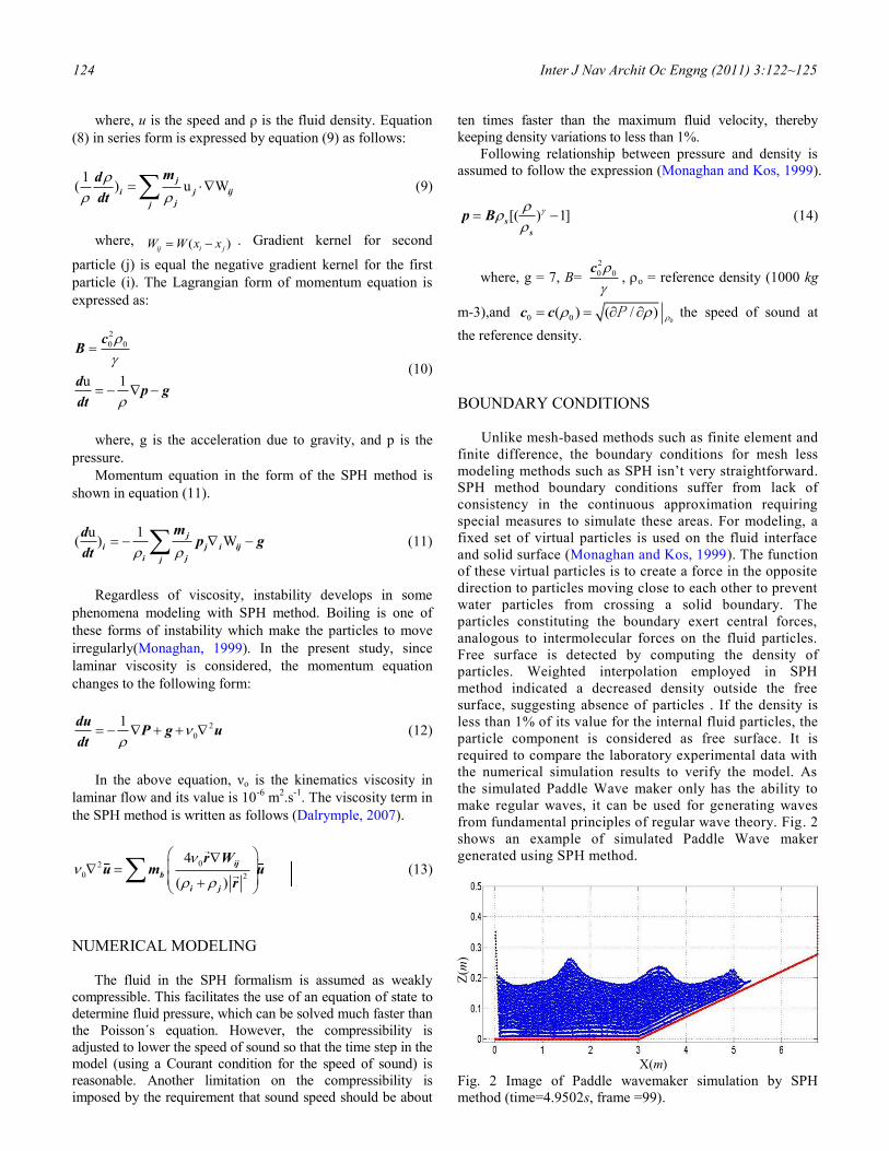
from fundamental principles of regular wave theory. Fig. 2

shows an example of simulated Paddle Wave maker

generated using SPH method.

Fig. 2 Image of Paddle wavemaker simulation by SPH

method (time=4.9502s, frame =99).

X(m)

Z(m

)

Inter J Nav Archit Oc Engng (2011) 3:122~125 125

To verify the results, the surface profiles are first

obtained with the theoretical values and compared with the

SPH simulation. Following the theories of wave maker, the

ratio of wave height to stroke of Paddle wave maker are

obtained by:

4sinh 1 coshsinh

sinh 2 2

H kh khkh

S kh kh kh (15)

where, H is the wave height, S is the wave stroke, k is the wave

number (= 2π / L where L is the wavelength), and h is the water

depth. Fig. 3 shows the image of a Paddle wave maker.

Fig. 3 Schematic picture of Paddle wave maker (flap type).

RESULTS AND DISCUSSIONS

Due to lack of laboratory data for Paddle wave maker, we

used the data available in the literature (Dalrymple, 2007).

For comparison of data, a second wave period of 5cm wave

height and 40cm depth of water was considered. The results

of SPH numerical model showed good agreement with the

experimental data (Fig. 4).

Fig. 4 Comparison of water surface profiles in laboratory data

and SPH model developed in this research.

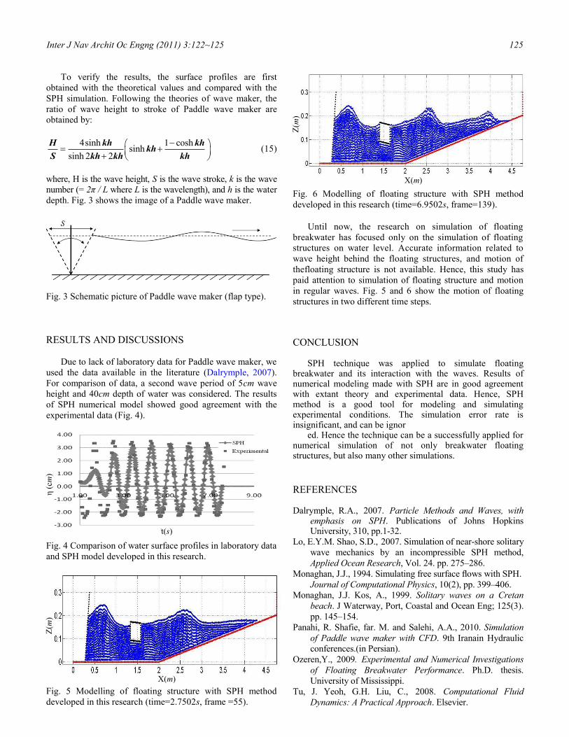
Fig. 5 Modelling of floating structure with SPH method

developed in this research (time=2.7502s, frame =55).

Fig. 6 Modelling of floating structure with SPH method

developed in this research (time=6.9502s, frame=139).

Until now, the research on simulation of floating

breakwater has focused only on the simulation of floating

structures on water level. Accurate information related to

wave height behind the floating structures, and motion of

thefloating structure is not available. Hence, this study has

paid attention to simulation of floating structure and motion

in regular waves. Fig. 5 and 6 show the motion of floating

structures in two different time steps. CONCLUSION

SPH technique was applied to simulate floating

breakwater and its interaction with the waves. Results of numerical modeling made with SPH are in good agreement with extant theory and experimental data. Hence, SPH method is a good tool for modeling and simulating experimental conditions. The simulation error rate is insignificant, and can be ignor

ed. Hence the technique can be a successfully applied for numerical simulation of not only breakwater floating structures, but also many other simulations.

REFERENCES

Dalrymple, R.A., 2007. Particle Methods and Waves, with

emphasis on SPH. Publications of Johns Hopkins University, 310, pp.1-32.

Lo, E.Y.M. Shao, S.D., 2007. Simulation of near-shore solitary

wave mechanics by an incompressible SPH method,

Applied Ocean Research, Vol. 24. pp. 275–286.

Monaghan, J.J., 1994. Simulating free surface flows with SPH.

Journal of Computational Physics, 10(2), pp. 399–406.

Monaghan, J.J. Kos, A., 1999. Solitary waves on a Cretan beach. J Waterway, Port, Coastal and Ocean Eng; 125(3).

pp. 145–154.

Panahi, R. Shafie, far. M. and Salehi, A.A., 2010. Simulation of Paddle wave maker with CFD. 9th Iranain Hydraulic

conferences.(in Persian).

Ozeren,Y., 2009. Experimental and Numerical Investigations of Floating Breakwater Performance. Ph.D. thesis.

University of Mississippi.

Tu, J. Yeoh, G.H. Liu, C., 2008. Computational Fluid Dynamics: A Practical Approach. Elsevier.

X(m)

Z(m

)

t(s)

η (

cm)

X(m)

Z(m

)