Embed Size (px)
Citation preview

U.S. Department of the InteriorU.S. Geological Survey
Scientific Investigations Report 2009–5205
Prepared in cooperation with the city of Rapid City
Numerical Groundwater-Flow Model of the Minnelusa and Madison Hydrogeologic Units in the Rapid City Area, South Dakota

Front cover. Swallow hole in Madison Limestone in Spring Creek Canyon (photograph by Ingrid E. Arlton).
Back cover. Doty Spring discharging from the Madison Limestone to Boxelder Creek (photograph by Ingrid E. Arlton).


Numerical Groundwater-Flow Model of the Minnelusa and Madison Hydrogeologic Units in the Rapid City Area, South Dakota
By Larry D. Putnam and Andrew J. Long
Prepared in cooperation with the city of Rapid City
Scientific Investigations Report 2009–5205
U.S. Department of the InteriorU.S. Geological Survey

U.S. Department of the InteriorKEN SALAZAR, Secretary
U.S. Geological SurveySuzette M. Kimball, Acting Director
U.S. Geological Survey, Reston, Virginia: 2009
For more information on the USGS—the Federal source for science about the Earth, its natural and living resources, natural hazards, and the environment, visit http://www.usgs.gov or call 1-888-ASK-USGS
For an overview of USGS information products, including maps, imagery, and publications, visit http://www.usgs.gov/pubprod
To order this and other USGS information products, visit http://store.usgs.gov
Any use of trade, product, or firm names is for descriptive purposes only and does not imply endorsement by the U.S. Government.
Although this report is in the public domain, permission must be secured from the individual copyright owners to reproduce any copyrighted materials contained within this report.
Suggested citation:Putnam, L.D., and Long, A.J., 2009, Numerical groundwater-flow model of the Minnelusa and Madison hydrogeologic units in the Rapid City area, South Dakota: U.S Geological Survey Scientific Investigations Report 2009–5205, 81 p.

iii
Contents
Abstract ...........................................................................................................................................................1Introduction.....................................................................................................................................................2
Purpose and Scope ..............................................................................................................................2Previous Investigations........................................................................................................................2Acknowledgments ................................................................................................................................2
Description of Study Area ............................................................................................................................4Physiography and Climate ...................................................................................................................4Hydrogeologic Setting .........................................................................................................................4
Minnelusa Hydrogeologic Unit ..................................................................................................8Madison Hydrogeologic Unit .....................................................................................................8
Numerical Groundwater-Flow Model .........................................................................................................9Finite-Difference Grid and Boundary Conditions ..........................................................................10Calibration and Simulated Stress Periods ......................................................................................14Representation of Flow-System Components ................................................................................18
Recharge .....................................................................................................................................19Streamflow Recharge ......................................................................................................19Areal Recharge .................................................................................................................20Upward Flow from Deadwood Aquifer ..........................................................................23
Discharge ....................................................................................................................................23Springflow ..........................................................................................................................23Water Use ..........................................................................................................................26Flow to Overlying Units ....................................................................................................26Regional Outflow ...............................................................................................................28
Hydraulic Properties .................................................................................................................28Horizontal Hydraulic Conductivity ..................................................................................28Vertical Hydraulic Conductivity ......................................................................................33Horizontal Flow Barriers ..................................................................................................37Storage Properties ...........................................................................................................37
Steady-State Calibration ...................................................................................................................39Sensitivity Analysis ....................................................................................................................39Comparison of Simulated and Observed Steady-State Hydraulic Head Values .............43Comparison of Simulated and Estimated Steady-State Flow .............................................43
Transient Calibration ..........................................................................................................................43Comparison of Simulated and Observed Transient Hydraulic Head Values ....................47Comparison of Simulated and Observed Transient Springflow .........................................53Comparison of Simulated and Estimated Transient Regional Outflow..............................53
Calibrated Hydraulic Properties .......................................................................................................53Response to Stress ......................................................................................................................................58Model Limitations.........................................................................................................................................58Summary........................................................................................................................................................60References Cited..........................................................................................................................................64Supplemental Information ..........................................................................................................................67

iv
Figures 1. Map showing location of study area .........................................................................................3 2. Stratigraphic section for the study area ...................................................................................5 3. Schematic showing conceptual hydrogeologic section of the study area ........................6 4. Generalized diagram with vertical exaggeration of a confined
aquifer recharged at the updip end ...........................................................................................7 5. Generalized diagram showing recharge conditions and vertical
gradients in the Minnelusa and Madison hydrogeologic units ............................................8 6. Conceptual schematic of model layers in relation to hydrogeology .................................10 7–12. Maps showing: 7. Location of finite-difference grid ....................................................................................11 8. Active model cells and boundary conditions for layers 1 and 2
(Minnelusa hydrogeologic unit) ......................................................................................12 9. Active model cells and boundary conditions for layers 3 and 4
(Madison hydrogeologic unit) ..........................................................................................13 10. Specified-flow cells representing streamflow recharge ............................................15 11. Model cells representing upward flow from the Deadwood aquifer
to layer 4, flow from the Minnelusa hydrogeologic unit to overlying units, and discharge to Elk Spings ..................................................................................16
12. Locations of head-dependent flow cells representing springs in the detailed study area ............................................................................................................17
13. Graph showing total transient streamflow recharge rates for twenty 6-month stress periods by model layer ...................................................................................21
14. Map showing locations of areal recharge zones..................................................................22 15. Graph showing total transient areal recharge rates for twenty 6-month
stress periods by model layer and spatially averaged precipitation on outcrops of the Minnelusa and Madison hydrogeologic units ...........................................24
16–26. Maps showing: 16. Locations of specified-flow cells representing water use in model
layers 1 and 3 ......................................................................................................................27 17. Horizontal hydraulic conductivity parameter groups and zones for
model layer 1 ......................................................................................................................29 18. Horizontal hydraulic conductivity multiplier zones for model layer 2 .......................30 19. Horizontal hydraulic conductivity parameter groups and zones for
model layer 3 ......................................................................................................................31 20. Horizontal hydraulic conductivity parameter groups and zones for
model layers 3 in the detailed study area ......................................................................32 21. Horizontal hydraulic conductivity multiplier zones for model layer 4 .......................34 22. Horizontal hydraulic conductivity parameter group for model
layer 5 and horizontal flow barriers for layers 1 to 5 ...................................................35 23. Vertical hydraulic conductivity parameter groups and zones for
model layer 2, transition zone for sulfate concentrations in Minnelusa hydrogeologic unit, and location of aquifer tests in Madison aquifer ......................36
24. Model cells with storage represented by unconfined storage coefficient ...........................................................................................................................38
v
25. Comparison of simulated steady-state potentiometric surface for model layer 1 to the average potentiometric surface of the Minnelusa aquifer, water years 1988–97 ...........................................................................................40
26. Comparison of simulated steady-state potentiometric surface for model layer 3 and western part of layer 4 to the average potentiometric surface of the Madison aquifer, water years 1988–97 .....................41
27–29. Graphs showing: 27. Composite-scaled sensitivities for parameter values that were
determined with inverse modeling in steady-state simulation ..................................43 28. Residuals between simulated steady-state and observed hydraulic
head values and their relation to average (water years 1988–97) hydraulic head values .......................................................................................................44
29. Histograms of residuals between simulated steady-state and observed (average for water years 1988–97) hydraulic head values .......................44
30–32. Maps showing: 30. Differences between simulated steady-state and observed (average
for water years 1988–97) hydraulic head values for the Minnelusa hydrogeologic unit in the detailed study area ..............................................................45
31. Differences between simulated steady-state and observed (average for water years, 1988–97) hydraulic head values for the Madison hydrogeologic unit in the detailed study area ..............................................................46
32. Locations of observation wells with transient hydraulic head values .....................48 33–34. Graphs showing: 33. Simulated and observed hydraulic head values for model layers 1
and 3 .....................................................................................................................................50 34. Simulated and observed or estimated springflow values ..........................................55 35. Map showing simulated extent of drawdown resulting from hypothetical
increases in pumping rates from the Madison hydrogeologic unit ...................................59 36. Graph showing simulated decrease in springflow from Jackson-Cleghorn
Springs in response to hypothetical increases in pumping rates from the Madison hydrogeologic unit .....................................................................................................60
37. Map showing locations of production and observation wells for Madison aquifer test at well 49 .................................................................................................................61
38. Graph showing simulated and observed drawdown for Madison aquifer test at well 49 ...............................................................................................................................62
Tables 1. Stress periods for transient simulations .................................................................................18 2. Estimated water-budget components for steady-state simulation ....................................19 3. Steady-state streamflow recharge rates distributed by model layer ................................20 4. Areal recharge zones and average annual precipitation on outcrops of
the Minnelusa and Madison hydrogeologic units .................................................................21 5. Areal recharge zones and steady-state areal recharge rates distributed
by model layer .............................................................................................................................23 6. Steady-state springflow ............................................................................................................25 7. Water-use rates for steady-state and transient simulations ..............................................26

vi
8. Sites used as basis for delineation of hydraulic conductivity parameter zones for model layer 3 ..............................................................................................................33
9. Horizontal barrier hydraulic characteristic for City Springs fault, City Springs monocline, and Victoria Creek fault ..........................................................................37
10. Composite-scaled sensitivities for hydraulic properties represented as parameters ...................................................................................................................................42
11. Steady-state springflow estimates and simulated springflow ...........................................47 12. Difference between simulated and observed hydraulic head values for
transient simulation ....................................................................................................................49 13. Estimated and simulated transient springflow ......................................................................54 14. Jackson-Cleghorn springflow estimated from streamflow measurements
on Rapid Creek ............................................................................................................................56 15. Simulated transient regional outflow from Minnelusa and Madison
hydrogeologic units at the eastern model boundary ............................................................56 16. Calibrated horizontal hydraulic conductivity for parameters representing
zones of hydraulic conductivity in model layers 1, 3, and 5 .................................................57 17. Conductance for head-dependent cells representing springs ...........................................57 18. Transient streamflow recharge rates for the Minnelusa and Madison
hydrogeologic units ....................................................................................................................68 19. Transient areal recharge rates for the Minnelusa and Madison
hydrogeologic units by zones ...................................................................................................70 20. Observed and simulated hydraulic head values for the Minnelusa
hydrogeologic unit in steady-state simulation .......................................................................71 21. Observed and simulated hydraulic head values for the Madison
hydrogeologic unit in steady-state simulation .......................................................................77 22. Supplemental interpolated hydraulic head values for the Minnelusa and
Madison hydrogeologic units in steady-state simulation ....................................................80

vii
Conversion Factors and Datums
Multiply By To obtain
Length
inch (in.) 2.54 centimeter (cm)foot (ft) 0.3048 meter (m)mile (mi) 1.609 kilometer (km)
Area
square mile (mi2) 259.0 hectare (ha)square mile (mi2) 2.590 square kilometer (km2)
Volume
gallon (gal) 3.785 liter (L) gallon (gal) 0.003785 cubic meter (m3) cubic foot (ft3) 0.02832 cubic meter (m3)
Flow rate
cubic foot per second (ft3/s) 0.02832 cubic meter per second (m3/s)gallon per minute (gal/min) 0.06309 liter per second (L/s)inch per year (in/yr) 25.4 millimeter per year (mm/yr)
Hydraulic conductivity
foot per day (ft/d) 0.3048 meter per day (m/d)
Conductance
feet squared per day (ft2/d) 0.0929 Meter squared per day (m2/d)
Temperature in degrees Fahrenheit (°F) may be converted to degrees Celsius (°C) as follows:
°C=(°F-32)/1.8
Vertical coordinate information is referenced to the National Geodetic Vertical Datum of 1929 (NGVD 29).
Horizontal coordinate information is referenced to the North American Datum of 1927 (NAD 27).
Altitude, as used in this report, refers to distance above the vertical datum.
Water year (WY) is the 12-month period, October 1 through September 30, and is designated by the calendar year in which it ends.
Abbreviations and Acronyms
SDDENR South Dakota Department of Environment and Natural Resources
SDME standard deviation of measurement error
USGS U.S. Geological Survey
WY water year


Numerical Groundwater-Flow Model of the Minnelusa and Madison Hydrogeologic Units in the Rapid City Area, South Dakota
By Larry D. Putnam and Andrew J. Long
AbstractThe city of Rapid City and other water users in the
Rapid City area obtain water supplies from the Minnelusa and Madison aquifers, which are contained in the Minnelusa and Madison hydrogeologic units. A numerical groundwater-flow model of the Minnelusa and Madison hydrogeologic units in the Rapid City area was developed to synthesize estimates of water-budget components and hydraulic properties, and to provide a tool to analyze the effect of additional stress on water-level altitudes within the aquifers and on discharge to springs. This report, prepared in cooperation with the city of Rapid City, documents a numerical groundwater-flow model of the Minnelusa and Madison hydrogeologic units for the 1,000-square-mile study area that includes Rapid City and the surrounding area.
Water-table conditions generally exist in outcrop areas of the Minnelusa and Madison hydrogeologic units, which form generally concentric rings that surround the Precambrian core of the uplifted Black Hills. Confined conditions exist east of the water-table areas in the study area.
The Minnelusa hydrogeologic unit is 375 to 800 feet (ft) thick in the study area with the more permeable upper part containing predominantly sandstone and the less permeable lower part containing more shale and limestone than the upper part. Shale units in the lower part generally impede flow between the Minnelusa hydrogeologic unit and the underlying Madison hydrogeologic unit; however, fracturing and weath-ering may result in hydraulic connections in some areas. The Madison hydrogeologic unit is composed of limestone and dolomite that is about 250 to 610 ft thick in the study area, and the upper part contains substantial secondary permeability from solution openings and fractures. Recharge to the Minn-elusa and Madison hydrogeologic units is from streamflow loss where streams cross the outcrop and from infiltration of precipitation on the outcrops (areal recharge).
MODFLOW–2000, a finite-difference groundwater-flow model, was used to simulate flow in the Minnelusa and Madison hydrogeologic units with five layers. Layer 1 represented the fractured sandstone layers in the upper 250 ft of the Minnelusa hydrogeologic unit, and layer 2 represented
the lower part of the Minnelusa hydrogeologic unit. Layer 3 represented the upper 150 ft of the Madison hydrogeologic unit, and layer 4 represented the less permeable lower part. Layer 5 represented an approximation of the underlying Dead-wood aquifer to simulate upward flow to the Madison hydro-geologic unit. The finite-difference grid, oriented 23 degrees counterclockwise, included 221 rows and 169 columns with a square cell size of 492.1 ft in the detailed study area that surrounded Rapid City. The northern and southern boundar-ies for layers 1–4 were represented as no-flow boundaries, and the boundary on the east was represented with head-dependent flow cells. Streamflow recharge was represented with specified-flow cells, and areal recharge to layers 1–4 was represented with a specified-flux boundary. Calibration of the model was accomplished by two simulations: (1) steady-state simulation of average conditions for water years 1988–97 and (2) transient simulations of water years 1988–97 divided into twenty 6-month stress periods.
Flow-system components represented in the model include recharge, discharge, and hydraulic properties. The steady-state streamflow recharge rate was 42.2 cubic feet per second (ft3/s), and transient streamflow recharge rates ranged from 14.1 to 102.2 ft3/s. The steady-state areal recharge rate was 20.9 ft3/s, and transient areal recharge rates ranged from 1.1 to 98.4 ft3/s. The upward flow rate from the Deadwood aquifer to the Madison hydrogeologic unit was 6.3 ft3/s. Discharge included springflow, water use, flow to overlying units, and regional outflow. The estimated steady-state spring-flow of 32.8 ft3/s from seven springs was similar to the simu-lated springflow of 31.6 ft3/s, which included 20.5 ft3/s from Jackson-Cleghorn Springs. Simulated transient springflow ranged from 25.7 to 42.3 ft3/s. Steady-state water-use rates for the Minnelusa and Madison hydrogeologic units were 3.4 and 6.7 ft3/s, respectively. Total transient water-use rates ranged from 3.4 to 19.1 ft3/s. Flow from the Minnelusa hydrogeologic unit to overlying units was 2.0 ft3/s. Steady-state and transient regional outflows from the Minnelusa and Madison hydrogeo-logic units were 12.9 and 12.8 ft3/s, respectively.
Linear regression of the 252 simulated and observed hydraulic head values for the steady-state simulation had a coefficient of determination (R2 value) of 0.92 with an average

2 Numerical Groundwater-Flow Model of the Minnelusa and Madison Hydrogeologic Units, Rapid City Area, S. Dak.
absolute difference of 37.6 ft. For the transient simulation, the average absolute difference between simulated and observed hydraulic head values for 19 observation wells ranged from 3.5 to 65.1 ft with a median value of 18.3 ft.
Calibrated horizontal hydraulic conductivity values for model layer 1 ranged from 1.0 to 5.2 feet per day (ft/d). Horizontal hydraulic conductivity values for model layer 3 ranged from 0.1 to 388.8 ft/d. Horizontal hydraulic conductiv-ity for layers 2 and 4 were 10 percent of hydraulic conductiv-ity values for layers 1 and layer 3, respectively, except near the outcrop where it was 50 percent of the values for layers 1 and 3, respectively. Vertical hydraulic conductivity for layers 1, 3, 4, and 5 was 10 percent of the respective horizontal hydraulic conductivity for those layers. Vertical hydraulic conductivity for layer 2 ranged from 0.000001 to 0.25 ft/d. Conductance for head-dependent cells representing springs ranged from 3,000 to 86,400 feet squared per day.
Simulation of increased hypothetical pumping of more than about 10 ft3/s may require modification of the boundaries to allow flow into the model. The model is limited by simpli-fying assumptions necessary to represent material having secondary porosity as a porous media. With additional data, further refinement of the model would be possible, which could improve the accuracy of model estimates of the effects of additional stresses on the system, such as increased with-drawals or drought. The model can yield simulations of future conditions, which can guide management decisions and plan-ning. The model provides a useful tool for general character-ization of the effects of stresses and management alternatives on a regional basis.
IntroductionThe city of Rapid City, South Dakota (fig. 1), obtains
more than one-half of its municipal water supplies from the Minnelusa and Madison aquifers through deep wells and springs, predominantly from the Madison aquifer. Numerous additional users in the Rapid City area obtain water from these aquifers for domestic, commercial, industrial, and irrigation usage. Groundwater flow within the Minnelusa and Madison aquifers is complex with extensive secondary porosity from fracturing, solution enhancement, and brecciation. The Minn-elusa and Madison aquifers are contained within the Minn-elusa and Madison hydrogeologic units, which include layers with less permeability.
The U.S. Geological Survey (USGS), as part of a long-term cooperative study with the city of Rapid City, has compiled numerous datasets designed to better understand groundwater flow in the Minnelusa and Madison hydro-geologic units. A numerical groundwater-flow model of the Minnelusa and Madison hydrogeologic units in the Rapid City area was developed to synthesize estimates of water-budget components and hydraulic properties, and to provide a tool to
analyze the effect of additional stress on water-level altitudes within the aquifers and on discharge to springs.
Purpose and Scope
The purposes of this report are to (1) document the development of a numerical groundwater-flow model of the Minnelusa and Madison hydrogeologic units, which contain the Minnelusa and Madison aquifers, in the Rapid City area in South Dakota, and (2) present simulated responses to stress and describe model limitations. The report describes the cali-brated numerical groundwater-flow model including estimates of recharge, discharge, and hydraulic properties that character-ize the Minnelusa and Madison hydrogeologic units.
Previous Investigations
This numerical modeling effort utilized datasets compiled in a report by Long and Putnam (2002) that documents a conceptual model of the Madison and Minnelusa aquifers. The concepts and datasets from that report were used exten-sively in constructing the numerical groundwater-flow model. Detailed description of the methods and interpretations that were used in compiling these datasets is available in Long and Putnam (2002). The conceptual-model report by Long and Putnam (2002) describes previous investigations perti-nent to this report. Previous investigations include several publications from the Black Hills hydrology study (Hortness and Driscoll, 1998; Carter and Redden, 1999a, 1999b, 1999c; Strobel and others, 1999; Driscoll, Bradford, and Moran, 2000; Driscoll, Hamade, and Kenner, 2000; Carter and others, 2001) and studies specific to the Rapid City area (Greene, 1993, 1999; Anderson and others, 1999; Long, 2000; Long and Putnam, 2002).
Recent studies of the Minnelusa and Madison aquifers include linear modeling of three components of flow in karst aquifers by using oxygen isotopes (Long and Putnam, 2004). Hargrave (2005) described the vulnerability of the Minnelusa aquifer to contamination. Miller (2005) described the influ-ences of geologic structures and stratigraphy on groundwater flow in the karstic Madison hydrogeologic unit in the study area. Putnam and Long (2007) characterized karst ground-water flow in the Rapid City area by using fluorescent dyes. Long and others (2008) described the use of age-determining tracers in conjunction with other tracers to characterize groundwater flow paths in the Madison aquifer.
Acknowledgments
The authors acknowledge the extensive support from the city of Rapid City for numerous studies from which data-sets used in this modeling effort have been developed. West Dakota Water Development District and the South Dakota School of Mines and Technology participated in numerous
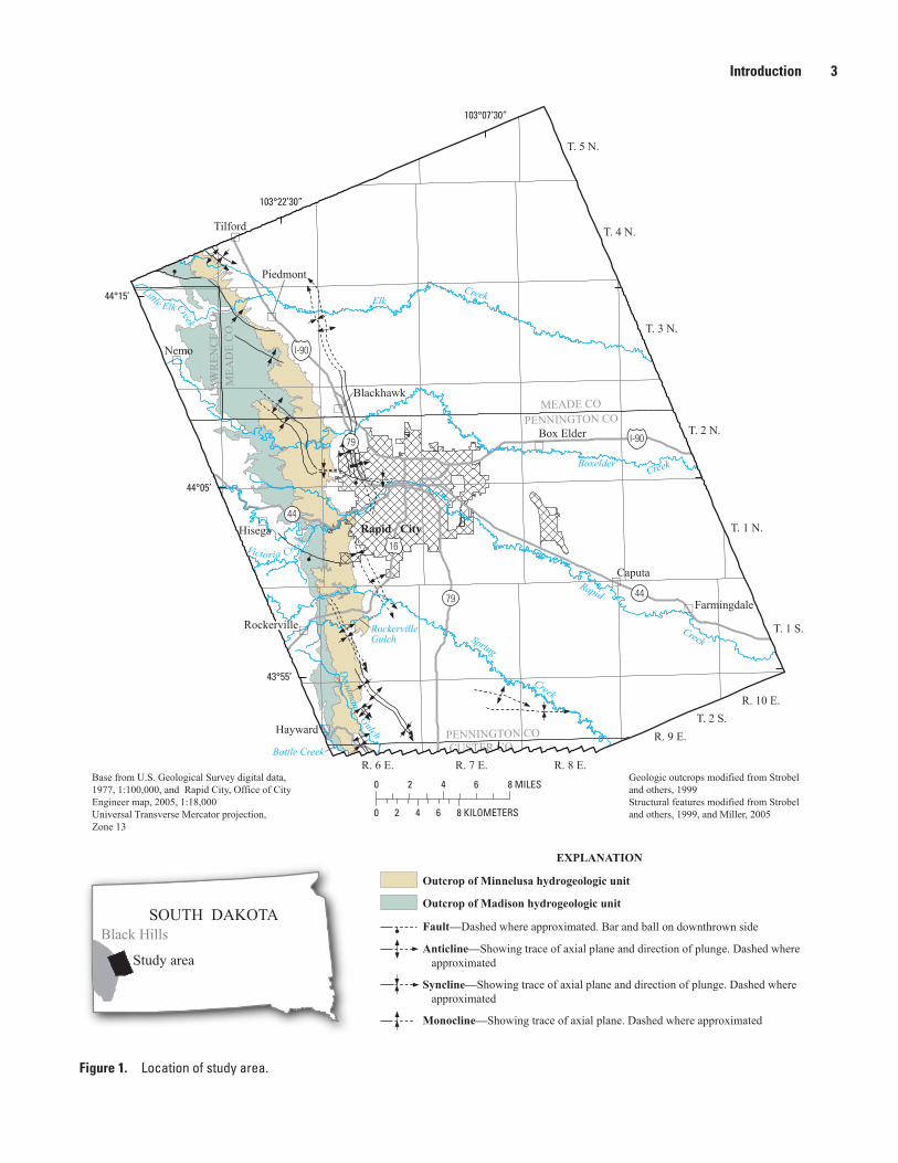
Figure 1. Location of study area.
MEADE CO
LAW
REN
CE
CO
PENNINGTON CO
MEA
DE
CO
PENNINGTON CO
CUSTER CO
SOUTH DAKOTA
Study area
Black Hills
Nemo
Caputa
Hisega
Hayward
Tilford
Piedmont
Box Elder
Blackhawk
Rockerville
Farmingdale
R. 8 E.
Elk
Boxelder
Rapid
Spring
Rapid CityGulch
Creek
T. 5 N.
T. 3 N.
T. 4 N.
T. 1 S.
T. 2 N.
T. 1 N.
T. 2 S.
R. 6 E. R. 7 E.
R. 9 E.
R. 10 E.
103°07’30”
103°22’30”
16
I-90
I-90
Creek
Creek
Creek
Creek
EXPLANATION
Outcrop of Minnelusa hydrogeologic unit
Outcrop of Madison hydrogeologic unit
Fault—Dashed where approximated. Bar and ball on downthrown side
Anticline—Showing trace of axial plane and direction of plunge. Dashed where approximated
Syncline—Showing trace of axial plane and direction of plunge. Dashed where approximated
Monocline—Showing trace of axial plane. Dashed where approximated
Base from U.S. Geological Survey digital data, 1977, 1:100,000, and Rapid City, Office of City Engineer map, 2005, 1:18,000 Universal Transverse Mercator projection, Zone 13
Geologic outcrops modified from Strobel and others, 1999Structural features modified from Strobel and others, 1999, and Miller, 2005
Victoria Creek
Deadm
an
Battle Creek
Little Elk
RockervilleGulch
43°55’
44°15’
44°05’
0 4 62 8 MILES
0 642 8 KILOMETERS
44
44
79
79
Introduction 3

4 Numerical Groundwater-Flow Model of the Minnelusa and Madison Hydrogeologic Units, Rapid City Area, S. Dak.
studies to better understand the complex hydrogeology in the Rapid City area. The Water Rights Program of the South Dakota Department of Environment and Natural Resources (SDDENR) provided compilations of water-level data for numerous observation wells they operate in the study area. The SDDENR also provided water-use data.
Description of Study AreaThe approximately 1,000-square-mile (mi2) study area
(fig. 1) on the eastern flank of the Black Hills includes Rapid City and the surrounding area. The study area extends from Elk Creek on the north to Battle Creek on the south, and from the outcrop of the Madison hydrogeologic unit on the west to Farmingdale and Box Elder on the east (fig. 1). The population of Rapid City in the 2000 census was 59,607 (U.S. Census Bureau, 2000). The area around Rapid City includes numer-ous suburban subdivisions and smaller towns. The study area includes parts of Lawrence, Meade, Pennington, and Custer Counties. The Minnelusa and Madison aquifers are important sources of water for many of the smaller communities and subdivisions in these counties.
Physiography and Climate
Land-surface altitudes range from more than 5,000 feet (ft) above the National Geodetic Vertical Datum of 1929 on the western side of the study area to about 2,800 ft near Farmingdale. The western extent of the study area is characterized by high relief covered predominantly by pine and spruce forests. The east ern lowlands are characterized by rolling prairies with bottom lands along stream channels. The Minnelusa and Madison hydrogeologic units crop out in the western part of study area along the eastern flank of the Black Hills uplift. These outcrops are characterized by high-relief forested areas cut by deep canyons with entrenched meanders and steep cliffs formed by resistant limestone and sandstone.
Average (water years 1961–90) precipitation rates range from about 24 inches per year (in/yr) in the northwest to about 16 in/yr in the eastern lowlands with most precipitation occur-ring in March, April, May, and June (Driscoll, Hamade, and Kenner, 2000). The average (1960–90) temperature at Rapid City is about 22 degrees Fahrenheit in January and about 72 degrees Fahrenheit in July (National Oceanic and Atmo-spheric Administration, 1996).
Hydrogeologic Setting
Uplift at the end of the Cretaceous period followed by erosion has created the dome-like structure and geomorphol-ogy of the Black Hills. Metamorphic and igneous rocks of Precambrian age are exposed in the Black Hills’ central core, whereas stratigraphic layers (figs. 2 and 3) of Paleozoic age
and younger are exposed on its flanks. The outcrops of Paleo-zoic units form generally concentric rings surrounding the Precambrian core and dip radially outward.
The Minnelusa and Madison hydrogeologic units dip away from the uplifted Black Hills at angles that can approach or exceed 15 to 20 degrees near the outcrops and decrease with distance from the uplift to less than 1 degree (Carter and Redden, 1999a, 1999b, 1999c). The Minnelusa and Madison aquifers are contained within the Minnelusa and Madison hydrogeologic units, and many studies refer to the aqui-fers as being the upper part of the hydrogeologic units. The Minnelusa hydrogeologic unit is composed of the Minnelusa Formation. The Madison hydrogeologic unit includes the Madison Limestone and the underlying Englewood Forma-tion because the Englewood Formation is hydrogeologically similar to the lower part of the Madison Limestone. The outcrop areas for the Minnelusa and Madison hydrogeologic units in the study area are about 39 square miles (mi2) and 52 mi2, respectively (fig. 1). Anticlines and synclines (fig. 1) result in local variations in the dip of beds near the outcrops.
A conceptual illustration of groundwater-flow compo-nents in an aquifer with hydrogeology similar to the Minn-elusa and Madison aquifers is shown in figure 4. Infiltrating precipita tion or streamflow losses may have an easterly flow component rather than a strictly vertical one because of the greater hydraulic conductivity parallel to easterly dipping bedding planes. The hydraulic head in the recharge area fluctuates with the changing recharge rate and causes a pressure wave to propagate through the confined part of the aquifer. This wave decreases in amplitude with distance traveled because of head losses in the aquifer. For this reason, hydraulic head fluctua tions in downgradient locations east of the recharge area generally are less than in the recharge area unless other stresses, such as pumping, are introduced. Springs discharge through breccias pipes, fractures, and enlarged solu-tion openings.
Water-table conditions generally exist in outcrop areas; however, the water table in the updip parts of the outcrops (approximately 1 to 2 miles along western edge) may be perched above the regional water table because of the higher altitudes. Recharge water may be stored under perched condi-tions before percolating downward to the regional water table. Water perched on dis continuous layers of low permeability material may exist in the Minnelusa Formation, and pools of perched water can be found in Madison Limestone caves. The unconfined area extends beyond the outcrop areas to the east a few hundred feet, where the dip is steepest, to more than 1 mile (mi), where the dip is less steep (Long and Putnam, 2002). Structural features near the outcrops (fig. 1) influence the shape and extent (described in the subsequent “Storage Properties” section) of the unconfined area. The estimated unconfined area is 36.3 mi2 for the Minnelusa hydrogeologic unit and 52.9 mi2 for the Madison hydrogeologic unit (Long and Putnam, 2002). East of the water-table areas, hydraulic head is above the tops of the hydrogeologic units owing to their easterly dip, and confined conditions exist. In some areas,

Figure 2. Stratigraphic section for the study area.
STRATIGRAPHIC UNIT DESCRIPTIONTHICKNESSIN FEET
ABBREVIATIONFOR
STRATIGRAPHICINTERVAL
SYSTEMERATHEM
QUATERNARY& TERTIARY (?)
UNDIFFERENTIATED SANDS AND GRAVELS 0–50 Sand, gravel, and boulders
1,200–2,000
Light colored clays with sandstone channel fillings and local limestone lenses.
Includes rhyolite, latite, trachyte, and phondite.
WHITE RIVER GROUP
INTRUSIVE IGNEOUS ROCKS
Tw
TuiTERTIARY
QTu
Principal horizon of limestone lenses giving teepee buttes.
Dark-gray shale containing scattered concretions.
Widely scattered limestone masses, giving small teepee buttes.
Black fissile shale with concretions.
PIERRE SHALE
NIOBRARA FORMATION 100–225 Impure chalk and calcareous shale.
CARLILE FORMATION Turner Sand MemberWall Creek Sands
400–750Light-gray shale with numerous large concretions and sandy layers.
Dark-gray shale.
GRAN
EROS
GRO
UP
GREENHORN FORMATION
Kps
25–380Impure slabby limestone. Weathers buff.
Dark-gray calcareous shale, with thin Orman Lake limestone at base.
BELLE FOURCHE SHALE
MOWRY SHALENEWCASTLESANDSTONE
SKULL CREEK SHALE
300–550Gray shale with scattered limestone concretions.
Clay spur bentonite at base.
150–250
20–60
Light-gray siliceous shale. Fish scales and thin layers of bentonite.
Brown to light-yellow and white sandstone.
170–270 Dark-gray to black siliceous shale.
CRETACEOUS
FALL RIVER FORMATION
LAKOTA FORMATION
INYA
N K
ARA
GROU
P10–200 Massive to slabby sandstone.
Coarse gray to buff crossbedded conglomeratic sandstone, interbedded with buff, red, and gray clay, especially toward top. Local fine-grained limestone.
35–700
0–220
0–225Green to maroon shale. Thin sandstone.Massive fine-grained sandstone.
250–450
0–45
Greenish-gray shale, thin limestone lenses.
Glauconitic sandstone; red sandstone near middle.
Red siltstone, gypsum, and limestone.
MORRISON FORMATION
UNKPAPA SS Redwater MemberLak MemberHulett MemberStockade Beaver Mem.Canyon Spr Member
SUNDANCEFORMATION
GYPSUM SPRING FORMATION
Kik
JuJURASSIC
Goose Egg EquivalentSPEARFISH FORMATIONT PsR
TRIASSIC
MINNEKAHTA LIMESTONEOPECHE SHALEPo
Pmk
250–700
125–65
Red sandy shale, soft red sandstone and siltstone with gypsum and thin limestone layers.Gypsum locally near the base.Thin to medium-bedded finely crystalline, purplish-gray laminated limestone.Red shale and sandstone.50-135
1,2375–800
2250–550
30–600–60
0–100
375–400
Yellow to red crossbedded sandstone, limestone, and anhydrite locally at top.
Red shale with interbedded limestone and sandstone at base.
Massive light-colored limestone. Dolomite in part. Cavernous in upper part.
Pink to buff limestone. Shale locally at base.Buff dolomite and limestone.Green shale with siltstone.Massive to thin-bedded buff to purple sandstone. Greenish glauconitic shale, flaggy dolomite, and flat-pebble limestone conglomerate. Sandstone, with conglomerate locally at the base.
Schist, slate, quartzite, and arkosic grit. Intruded by diorite, metamorphosed to amphibolite, and by granite and pegmatite.
PERMIAN
PENNSYLVANIAN
MISSISSIPPIAN
MINNELUSA FORMATION
MADISON (PAHASAPA) LIMESTONE
ENGLEWOOD FORMATION
MDme
Ou
DEVONIANWHITEWOOD (RED RIVER) FORMATIONWINNIPEG FORMATION
DEADWOOD FORMATION
UNDIFFERENTIATED METAMORPHICAND IGNEOUS ROCKS
OCd
pCu
ORDOVICIAN
CAMBRIAN
PRECAMBRIAN
PALE
OZOI
CM
ESOZ
OIC
CEN
OZOI
C
Modified from information furnished by the Department of Geology and Geological Engineering,South Dakota School of Mines and Technology (written commun., January 1994)
0–600
Interbedded sandstone, limestone, dolomite, shale, and anhydrite.
1 Modified on the basis of drill-hole data.
3 Based on Carter and others, 2001.
2 Thickness based on structure contours of Minnelusa Formation,Madison Limestone, and Deadwood Formation tops (Carter andRedden, 1999a, 1999b, 1999c).
MUDDYSANDSTONE
P Pm
Unknown
Description of Study Area
5

Figure 3. Conceptual hydrogeologic section of the study area (modified from Hayes, 1999). Each aquifer shown is separated from other aquifers by confining units. Hydraulic connection between aquifers is increased by vertical breccia pipes and fractures. The schematic shows (1) exposed breccia pipe above hydraulic head in Madison aquifer, (2) exposed breccia pipe with hydraulic head below land surface, (3) breccia pipe at active spring-discharge point, (4) developing breccia pipe, (5) fractures in confining unit, (6) breccia pipe originating in the Madison Limestone, (7) breccia pipe extending from Minnelusa Formation to the Inyan Kara Group, and (8) discontinuous residual clay soil. Arrows show general areal leakage, focused leakage at breccia pipes, or groundwater-flow directions.
WestEast
Potentiometric surfaceof Madison aquifer
Alluvium
Dip of sedimentary rocks greatly exaggerated
Precambrian metamorphic
and igneous rocks
Deadwood
Inyan Kara Group
Thicknesses not to scale
Madison
Minnelusa
Minnekahta
Limestone
Aquifer CaveBreccia pipeResidual clay soil (collapsed area)
Confining unit
EXPLANATION
Formation
Formation
Watertable
(1)
(2)
(3)
(4)
(5)
(6)
(8)
(7)
Limestone
Spring
Englewood Formation
6 Numerical Groundwater-Flow Model of the Minnelusa and Madison Hydrogeologic Units, Rapid City Area, S. Dak.
the hydraulic head is above the land surface, and flowing wells may exist in these areas. Hydraulic connection to the overly-ing Minnekahta Limestone and Inyan Kara Group is limited by intervening shale layers.
Movement of groundwater between the Minnelusa and Madison aquifers is influenced by vertical hydraulic gradients, hydraulic properties of the inter vening confining unit, and recharge rates (fig. 5; Long and Putnam, 2002). Although the confining units generally do not transmit water at a high rate, their capacity to store water could have substantial effects on
the hydraulics of the groundwater-flow system. Water that flows between the Minnelusa and Madison aquifers must pass through a confining unit that is several hundred feet thick with variable porosity and potentially a sub stantial amount of water held in storage. The confining units contain more secondary porosity in the western side of the study area where fractur-ing from the Black Hills uplift is more prevalent than in the eastern side of the study area. East of Rapid City, the hydraulic head is higher in the Minnelusa aquifer than in the Madison aquifer.

Figure 4. Generalized diagram with vertical exaggeration of a confined aquifer recharged at the updip end (from Long and Putnam, 2002). The diagram shows (1) recharge infiltrates and moves downward vertically or diagonally parallel to bedding planes, (2) near horizontal flow with head losses resulting from resistance from aquifer material, (3) sloping potentiometric surface results from head losses, (4) artesian spring discharges through high-conductivity breccia pipe or fracture because hydraulic head is above the land surface, (5) spring causes depression in the potentiometric surface, (6) outflow rate is controlled by hydraulic gradient and transmissivity, (7) hydraulic head fluctuation at recharge area is controlled by changes in recharge rate, and (8) smaller hydraulic head fluctuation downgradient is in response to larger fluctuation at recharge area.
Water table4
53
2
1
7
Areal recharge or infiltration
Unsaturated zone
Bedding plane
EXPLANATION
AquiferConfining unit
Confining unit
Outcropunsaturated
area
Outcrop area
Unconfinedarea Confined area
Direction of flow
Breccia pipe
8
6
Land surface
Losi
ngst
ream
West East
Potentiometric surface
Description of Study Area 7
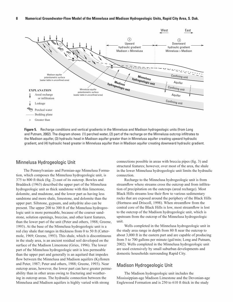
Figure 5. Recharge conditions and vertical gradients in the Minnelusa and Madison hydrogeologic units (from Long and Putnam, 2002). The diagram shows (1) perched water, (2) part of the recharge on the Minnelusa outcrop infiltrates to the Madison aquifer, (3) hydraulic head in Madison aquifer greater than in Minnelusa aquifer creating upward hydraulic gradient, and (4) hydraulic head greater in Minnelusa aquifer than in Madison aquifer creating downward hydraulic gradient.
West East
Minnelusa aquiferpotentiometric surface
(water table in unconfined area)
Madison aquiferpotentiometric surface
(water table in unconfined area)
43
1
Areal recharge or infiltration
Leakage
Perched waterBedding plane
EXPLANATION
Aquifer
Aquifer
Confining unit
Confining unit
Confining unitMadisonhydrogeologic unit
Minnelusahydrogeologic unit
Upwardhydraulic gradient
Madison > Minnelusa
Downwardhydraulic gradient
Minnelusa > Madison
Greater than
2
>
8 Numerical Groundwater-Flow Model of the Minnelusa and Madison Hydrogeologic Units, Rapid City Area, S. Dak.
Minnelusa Hydrogeologic Unit
The Pennsylvanian- and Permian-age Minnelusa Forma-tion, which composes the Minnelusa hydrogeologic unit, is 375 to 800 ft thick (fig. 2) east of its outcrop. Bowles and Braddock (1963) described the upper part of the Minnelusa hydrogeologic unit as thick sandstone with thin limestone, dolomite, and mudstone, and the lower part as having less sandstone and more shale, limestone, and dolomite than the upper part. Siltstone, gypsum, and anhydrite also can be present. The upper 200 to 300 ft of the Minnelusa hydrogeo-logic unit is more permeable, because of the coarser sand-stone, solution openings, breccias, and other karst features, than the lower part of the unit (Peter and others, 1988; Greene, 1993). At the base of the Minnelusa hydrogeologic unit is a red clay shale that ranges in thickness from 0 to 50 ft (Catter-mole, 1969; Greene, 1993). This shale, which is discontinuous in the study area, is an ancient residual soil developed on the surface of the Madison Limestone (Gries, 1996). The lower part of the Minnelusa hydrogeologic unit is less permeable than the upper part and generally is an aquitard that impedes flow between the Minnelusa and Madison aquifers (Kyllonen and Peter, 1987; Peter and others, 1988; Greene, 1993). Near outcrop areas, however, the lower part can have greater perme-ability than in other areas owing to fracturing and weather-ing in outcrop areas. The hydraulic connection between the Minnelusa and Madison aquifers is highly varied with strong
connections possible in areas with breccia pipes (fig. 3) and structural features; however, over most of the area, the shale in the lower Minnelusa hydrogeologic unit limits the hydraulic connection.
Recharge to the Minnelusa hydrogeologic unit is from streamflow where streams cross the outcrop and from infiltra-tion of precipitation on the outcrops (areal recharge). Most Black Hills streams lose their flow to various sedimentary rocks that are exposed around the periphery of the Black Hills (Hortness and Driscoll, 1998). When streamflow from the central core of the Black Hills is low, most streamflow is lost to the outcrop of the Madison hydrogeologic unit, which is upstream from the outcrop of the Minnelusa hydrogeologic unit.
Wells completed in the Minnelusa hydrogeologic unit in the study area range in depth from 80 ft near the outcrop to about 3,000 ft in the eastern part and are capable of producing from 5 to 700 gallons per minute (gal/min; Long and Putnam, 2002). Wells completed in the Minnelusa hydrogeologic unit are used extensively by small suburban developments and domestic households surrounding Rapid City.
Madison Hydrogeologic UnitThe Madison hydrogeologic unit includes the
Mississippian-age Madison Limestone and the Devonian-age Englewood Formation and is 250 to 610 ft thick in the study

Numerical Groundwater-Flow Model 9
50 gal/min, 11 percent yield 50 to 200 gal/min, and 25 percent yield 200 to 2,500 gal/min. The depth of wells ranges from 20 to 4,600 ft, with 78 percent of the wells less than 1,000 ft and 41 percent less than 500 ft (Long and Putnam, 2002). The deepest wells are on the eastern side of the study area, where the water level may be only a few hundred feet below the land surface owing to artesian pressure. The varied well yields are influenced by karst features, with the larger production wells connected to substantial solution openings.
Numerical Groundwater-Flow ModelMODFLOW–2000, a numerical, three-dimensional,
finite-difference groundwater-flow model (Harbaugh and others, 2000), was used to simulate flow in the hydrogeo-logic units within the study area. Detailed descriptions of MODFLOW–2000 packages that were used in the model are presented in McDonald and Harbaugh (1988) and Harbaugh and others (2000). The MODFLOW–2000 parameter estima-tion process (Hill and others, 2000) was used to optimize estimates of hydraulic properties for calibration.
The design of the numerical groundwater-flow model was based on the conceptual model described in Long and Putnam (2002) and includes five model layers (fig. 6). The Minnelusa and Madison hydrogeologic units were each represented by two model layers. Although the entire thickness of these units may include secondary porosity, the more permeable parts of the hydrogeologic units generally occur in the upper part of both units (Long and Putnam, 2002). Layer 1 represents the fractured sandstone layers in the upper part of the Minn-elusa hydrogeologic unit. The Minnelusa aquifer generally is contained in the upper 200 to 300 ft of the unit (Greene, 1993). Layer 2 represents the fractured limestone, minor sandstone layers, and shale units in the lower part of the Minnelusa hydrogeologic unit. Layer 3 represents the secondary porosity and karstic features of the Madison hydrogeologic unit that are more prevalent in the upper part than in the lower part. This layer approximates the upper two geomorphic units of the Madison Limestone described by Miller (2005) and described by Greene (1993) as being 100 to 200 ft thick in total. Layer 4 represents the less permeable lower part of the Madison hydrogeologic unit. Layer 5 represents the western part of the Deadwood aquifer to approximate upward flow to the Madison hydrogeologic unit from the underlying Deadwood aquifer. The Whitewood and Winnipeg Formations shown in figure 2 are absent throughout most of the study area (Long and Putnam, 2002).
Arrays representing the altitude of the tops of model layers 1, 3, and 5 were constructed from maps of the struc-tural tops of the Minnelusa Formation, Madison Limestone, and Deadwood Formation (Carter and Redden, 1999a, 1999b, 1999c; Long and Putnam, 2002). A uniform thickness of 250 ft was assumed for layer 1 with the remainder of the Minnelusa hydrogeologic unit represented as layer 2. The upper 250 ft
area. The Madison Limestone is composed of limestone and dolomite and is 250 to 550 ft thick east of the outcrop of the Madison hydrogeologic unit (fig. 2). The Englewood Forma-tion, which underlies the Madison Limestone, is less than 60 ft thick, is composed of argillaceous, dolomitic limestone, and probably could logically be considered a member of the Madison Limestone because of its lithology (Gries and Martin, 1985).
The upper surface of the Madison Limestone is a weathered karst surface and is unconformably overlain by the Minnelusa Formation (Cattermole, 1969). The upper 150 ft of the Madison hydrogeologic unit contains substantial secondary permeability from solution openings and fractures (Greene, 1993), and solution enlargement of fractures has resulted in a predominance of conduit flow. Secondary permeability in the lower part of the Madison hydrogeologic unit generally is smaller than in the upper part (Greene, 1993); however, the lower unit can have greater permeability near outcrop areas than in the eastern part, especially along stream channels.
The Madison Limestone was divided into four cliff-forming geomorphic units by Miller (2005) through detailed mapping of the canyons in the Spring, Rapid, and Boxelder Creek Basins that are on the west-central edge of the study area (fig. 1). The thickness of the units from bottom to top are 130 to 165 ft for unit 1, 81 to 120 ft for unit 2, 140 to 150 ft for unit 3, and 0 to 85 ft for unit 4. Late Mississippian erosion removed the upper part of unit 4 in the Boxelder and Spring Creek canyons and all of unit 4 and part of unit 3 in the Rapid Creek canyon. Unit 1 is highly resistant to erosion, having thickly bedded sections and forming nearly vertical cliffs. Unit 2 is similar; however, the bedding is thinner and cliff faces tend to be more irregular. Unit 3 is characterized by massive collapse brecciation with large angular blocks and poorly preserved bedding. Caves are numerous in unit 3 and commonly are filled with cemented solution breccias and cave fill. Unit 4, where present, is characterized by collapse brecciation with angular blocks. Upper cliff surfaces in unit 4 are rounded off because of low resistance to erosion. Karst features are located throughout the Madison Limestone; however, they tend to be more common along the contacts between these geomorphic units (Miller, 2005).
Recharge to the Madison hydrogeologic unit is from streamflow loss where streams cross the outcrops and from infiltration of precipitation on the outcrops. The streamflow loss threshold represents the maximum amount of streamflow loss that can occur when water is available in the stream. Loss thresholds for the major streams in the study area (Hortness and Driscoll, 1998) for the Madison hydrogeologic unit range from about 10 to 25 cubic feet per second (ft3/s). Because the Madison hydrogeologic unit outcrop is the most upstream unit with large loss thresholds, streamflow recharge is substantial and usually greater than areal recharge to the Madison hydro-geologic unit in the study area.
Wells completed in the Madison hydrogeologic unit in the study area are capable of producing from 5 to 2,500 gal/min. About 64 percent of the wells yield 5 to

Figure 6. Conceptual schematic of model layers in relation to hydrogeology.
Deadwood aquifer
Madison confining unit (includes Englewood Formation)
Minnelusaconfining
unit
Minnelusa aquifer
Madison aquifer
Spring Wells
Water use Discharge tooverlying units
Disc
harg
e by
regi
onal
out
flow
EXPLANATION
Aquifer
Confining unit
Well
Breccia pipe
Flow direction Areal recharge
Streamflow recharge
Model layer
2
1
3
4
5
Mad
ison
hyd
roge
olog
icun
it M
inne
lusa
hyd
roge
olog
icun
it
10 Numerical Groundwater-Flow Model of the Minnelusa and Madison Hydrogeologic Units, Rapid City Area, S. Dak.
generally contains the sandstone layers. The thickness of layer 2 ranged from 106 to 590 ft with a mean of 293 ft. A uniform thickness of 150 ft was assumed for layer 3 with the remainder of the Madison hydrogeologic unit represented in layer 4. The thickness of layer 4 ranged from 139 to 599 ft with a mean of 341 ft.
Finite-Difference Grid and Boundary Conditions
The finite-difference grid defining the model area consisted of 221 rows and 169 columns (fig. 7). The cell size was 492.1 ft (150 meters) by 492.1 ft in the detailed study area that surrounded Rapid City. Cell sizes increased from the detailed area to 1,640 ft in width at the boundaries on the north and south and to 6,562 ft in width at the boundary on the east (fig. 7). The model was oriented 23 degrees counterclockwise so that the orientation of finite-difference cells approximated the orthogonal patterns in cave passageways and fracture patterns (Greene and Rahn, 1995). This orientation allowed for simulation of horizontal anisotropy if necessary. Miller (2005) mapped a major trend in fractures and joints in the study area
as north 65 degrees east with a less dominant trend of north 35 degrees west. The general pattern of structural features (fig. 1; Strobel and others, 1999) in the study area was about 23 degrees.
The boundary conditions used in the model are described in general terms in this section with quantitative descriptions presented in the subsequent “Representation of Flow System Components” section. The mathematical concepts for various types of cells used to represent boundaries are described in detail in McDonald and Harbaugh (1988), and the specific MODFLOW–2000 packages that were used are included with the model cell descriptions that follow.
Boundaries on the north and south for layers 1–4 were represented as no-flow boundaries (figs. 8 and 9) because the northern and southern boundaries generally occur along flow lines. The boundaries on the east for layers 1–4 were represented with head-dependent flow cells (Drain Package, McDonald and Harbaugh, 1988). With this type of bound-ary cell, flow across the boundary changes in relation to the hydraulic head in the aquifer. The calculated flow is the differ-ence between a specified head and the head in the model cell multiplied by the area of the cell multiplied by the assigned
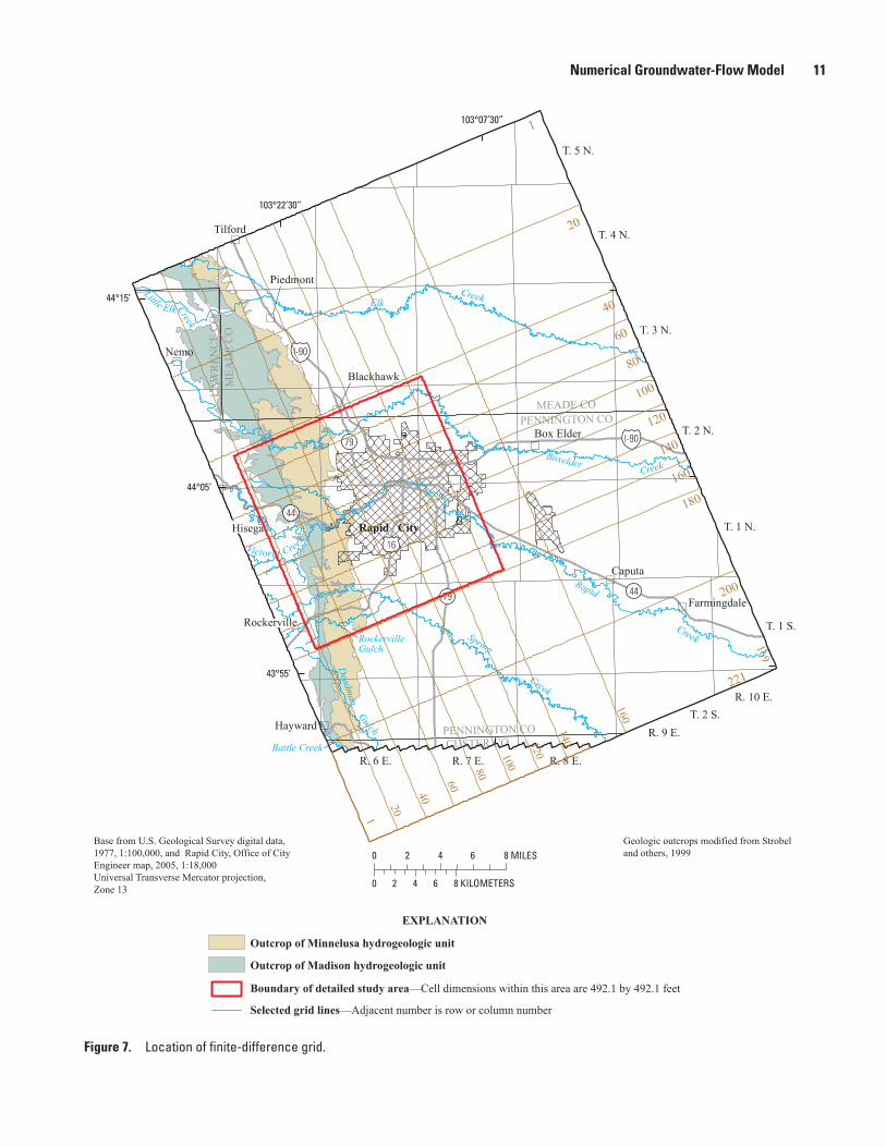
Figure 7. Location of finite-difference grid.
MEADE CO
LAW
REN
CE
CO
PENNINGTON CO
MEA
DE
CO
PENNINGTON CO
CUSTER CO
Nemo
Caputa
Hayward
Tilford
Piedmont
Box Elder
Blackhawk
Rockerville
Farmingdale
R. 8 E.
Elk
Boxelder
Rapid
Spring
Rapid CityGulch
Creek
T. 5 N.
T. 3 N.
T. 4 N.
T. 1 S.
T. 2 N.
T. 1 N.
T. 2 S.
R. 6 E. R. 7 E.
R. 9 E.
R. 10 E.
103°07’30”
103°22’30”
16
I-90
I-90
Creek
Creek
Creek
Creek
Victoria Creek
Deadm
an
Battle Creek
Little Elk
RockervilleGulch
Base from U.S. Geological Survey digital data, 1977, 1:100,000, and Rapid City, Office of City Engineer map, 2005, 1:18,000 Universal Transverse Mercator projection, Zone 13
Hisega
43°55’
44°15’
44°05’
0 4 62 8 MILES
0 642 8 KILOMETERS
44
44
79
79
1
20
40
60
80
100
120
140
160
180
200
221
1
60
20
80
40
169
120
140
160
100
EXPLANATION
Outcrop of Minnelusa hydrogeologic unit
Outcrop of Madison hydrogeologic unit
Boundary of detailed study area—Cell dimensions within this area are 492.1 by 492.1 feet
Selected grid lines—Adjacent number is row or column number
Geologic outcrops modified from Strobel and others, 1999
Numerical Groundwater-Flow Model 11

Figure 8. Active model cells and boundary conditions for layers 1 and 2 (Minnelusa hydrogeologic unit).
MEADE CO
LAW
REN
CE
CO
PENNINGTON CO
MEA
DE
CO
PENNINGTON CO
CUSTER CO
Nemo
Caputa
Hisega
Hayward
Tilford
Piedmont
Box Elder
Blackhawk
Rockerville
Farmingdale
R. 8 E.
Elk
Boxelder
Rapid
Spring
RapidCity
Gulch
Creek
T. 5 N.
T. 3 N.
T. 4 N.
T. 1 S.
T. 2 N.
T. 1 N.
T. 2 S.
R. 6 E. R. 7 E.
R. 9 E.
R. 10 E.
103°07’30”
103°22’30”
16
I-90
I-90
Creek
Creek
Creek
Creek
Base from U.S. Geological Survey digital data, 1977, 1:100,000, and Rapid City, Office of City Engineer map, 2005, 1:18,000 Universal Transverse Mercator projection, Zone 13
Victoria Creek
Deadman
Battle Creek
Little Elk
RockervilleGulch
43°55’
44°15’
44°05’
79
0 4 62 8 MILES
0 642 8 KILOMETERS
44
4479
EXPLANATION
Part of Minnelusa hydrogeologic unit estimated as unsaturated (inactive cells)
Active cells in layers 1 and 2
Active cells in layer 2
No-flow boundary
Head-dependent flow boundary representing outflow from layers 1 and 2
Specified-flux boundary representing areal recharge to layer 2 (applied to westernmost active cell in layer 2)
Specified-flux boundary representing areal recharge to layer 1 (applied to westernmost active cell in layer 1)
Minnelusa aquifer potentiometric contour (average for water years 1988–97; Long and Putnam, 2002)—Shows altitude at which water would have stood in tightly cased, nonpumped well. Contour interval 100 feet. Datum is National Geodetic Vertical Datum of 1929
3,500
2,600
2,700
2,8002,900
3,000
3,100
3,200
3,3,00
3,400
3,500
3,600
3,70
03,
800
2,900
3,000
3,1003,200
3,3,00
3,400
3,500
12 Numerical Groundwater-Flow Model of the Minnelusa and Madison Hydrogeologic Units, Rapid City Area, S. Dak.

Figure 9. Active model cells and boundary conditions for layers 3 and 4 (Madison hydrogeologic unit).
MEADE CO
LAW
REN
CE
CO
PENNINGTON CO
MEA
DE
CO
PENNINGTON CO
CUSTER CO
Nemo
Caputa
Hisega
Hayward
Tilford
Piedmont
Box Elder
Blackhawk
Rockerville
Farmingdale
R. 8 E.
Elk
Boxelder
Rapid
Spring
RapidCity
Gulch
Creek
T. 5 N.
T. 3 N.
T. 4 N.
T. 1 S.
T. 2 N.
T. 1 N.
T. 2 S.
R. 6 E. R. 7 E.
R. 9 E.
R. 10 E.
103°07’30”
103°22’30”
43°55’
44°15’
44°05’
16
I-90
I-90
Creek
Creek
Creek
Creek
Victoria Creek
Deadman
Battle Creek
Little Elk
RockervilleGulch
Base from U.S. Geological Survey digital data, 1977, 1:100,000, and Rapid City, Office of City Engineer map, 2005, 1:18,000 Universal Transverse Mercator projection, Zone 13
79
0 4 62 8 MILES
0 642 8 KILOMETERS
44
4479
EXPLANATION
Part of Madison hydrogeologic unit estimated as unsaturated (inactive cells)
Active cells in layers 3 and 4
Active cells in layer 4
No-flow boundary
Head-dependent flow boundary representing outflow from layers 3 and 4
Specified-flux boundary representing areal recharge to layer 4 (applied to westernmost active cell in layer 4)
Specified-flux boundary representing areal recharge to layer 3 (applied to westernmost active cell in layer 3)
Madison aquifer potentiometric contour (average for water years 1988–97; Long and Putnam, 2002)—Shows altitude at which water would have stood in tightly cased, nonpumped well. Contour interval 100 feet. Datum is National Geodetic Vertical Datum of 1929
3,500
3,50
0
3,40
0
3,300 3,200
3,100
3,000
2,900
2,800
2,700
2,600
3,9004,100
3,800
2,500
3,7003,600
3,5003,400
3,3003,200
3,100
3,000
2,900
2,80
02,7
00
2,600
3,60
03,
500
4,000
Numerical Groundwater-Flow Model 13

14 Numerical Groundwater-Flow Model of the Minnelusa and Madison Hydrogeologic Units, Rapid City Area, S. Dak.
boundary conductance. Conductance is a term that represents the hydraulic conduc tivity multiplied by a unit of length, and is expressed in units of feet squared per day (ft2/d). The bound-aries on the north, east, and south perimeters were located about 12 mi from the detailed study area to minimize their influence on analysis of groundwater flow in the detailed study area (fig. 7).
Areal recharge to layers 1–4 (figs. 8 and 9) was repre-sented with a specified-flux boundary (Recharge Package, McDonald and Harbaugh, 1988) with the recharge flux assigned to the westernmost active cell. Groundwater flow in the western part of the outcrops of the Minnelusa and Madison hydrogeologic units was not simulated for the unsaturated areas (figs. 8 and 9). In these areas near the outcrops, ground-water flow includes unsaturated areas, perched water, and caves intermittently filled with water that spills and moves downgradient. This non-Darcian flow was not simulated; therefore, accumulated infiltration of precipitation on the outcrop was assigned to the first downgradient (westernmost) active model cells in layers 1–4. Streamflow recharge was represented with specified-flow cells assigned to selected cells in layers 1–4 to represent streamflow loss that occurred when streams crossed the outcrops of the Minnelusa and Madison hydrogeologic units (fig. 10). Streamflow loss for the larger streams was gaged and described in Hortness and Driscoll (1998). The streamflow recharge cells were located approximately where streamflow loss was observed for the larger streams. For some streams, the specified-flow cells were moved downstream to the westernmost active cell in the model layer.
A specified-flux boundary (Recharge Package, McDon-ald and Harbaugh, 1988) representing the source of water for upward flow from the Deadwood aquifer (layer 5) to layer 4 was assigned to the westernmost active cells in layer 5 (fig. 11). Active cells for layer 5 extend from one cell west of active cells in layer 4 to the east beyond the start of active cells in layer 3 (fig. 11) with no-flow boundaries on the north, east, and south. The purpose of layer 5 was to approximate the distribution of upward flow from underlying units to the Madison hydrogeologic unit and not to simulate ground-water flow in the Deadwood aquifer. Upward flow from the Minnelusa hydrogeologic unit to overlying units, which was assumed to be small, was represented with specified-flux cells (Recharge Package, McDonald and Harbaugh, 1988) in the western part of the model where more fracturing was likely (Long and Putnam, 2002; fig. 11).
Springs discharging from the Minnelusa and Madison hydrogeologic units (figs. 11 and 12) were represented with head-dependent flow cells (Drain package or River Package, McDonald and Harbaugh, 1998). The user-specified hydrau-lic head at the cell or cells was set at the altitude of the land surface at the spring. The springs generally appear as seepage from the alluvium along streams; therefore, spring-flow through the bedrock openings could emerge somewhat upgradient from observed flow in the streams. A more detailed
description of individual springs and estimates of spring discharge is included in the subsequent “Springflow” section.
Calibration and Simulated Stress Periods
Calibration of the model was accomplished by two simu-lations: (1) steady-state simulation of average conditions for water years (WY) 1988–97 and (2) transient simulations for WY 1988–97 divided into twenty 6-month stress periods. The model was calibrated with both the steady-state and transient simulations by comparison of hydraulic head values and flows. Average hydraulic heads for water years 1988–97 (Long and Putnam, 2002) were assumed to approximate hydraulic heads for the steady-state simulation because the 10-year period included a range of hydrologic conditions. Hydraulic heads from the steady-state simulation were used as starting heads for the transient simulation. The transient stress periods (table 1) include a dry period in the late 1980s and early 1990s (stress periods 1–11) and a wet period in the late 1990s (stress periods 12–20). Most recharge occurred during the summer stress periods from April through September, and water use from the Madison aquifer also increased substantially during the summer stress periods. Recharge and other model compo-nents are described with more detail in the subsequent “Repre-sentation of Flow-System Components” section.
Inverse modeling with the MODFLOW–2000 param-eter estimation process (Hill and others, 2000) was used to calibrate the steady-state model, and trial-and-error methods were used to conjunctively calibrate the transient model. The term “parameter” in this report is used to describe any physical property that was estimated by model calibration. An “observation” is a direct measurement or an estimate based on measured data. A parameter can represent a particular property for a single cell or group of model cells. Simulated results were compared to measured or estimated hydraulic heads or flow rates and optimized.
In inverse modeling, simulated values of hydraulic head and flows are statistically compared to observed values. The program adjusts parameter values in an iterative process to produce the best possible match between the observed and simulated values. Parameterization is the process of identify-ing the aspects of the simulated system that can be optimized with these statistical algorithms. The number of parameters that can be estimated is limited by the amount and distribution of observed data (Hill, 1998). Some parameters may be insen-sitive to the observed data, or some parameters may be highly correlated with each other and cannot be optimized. The selection of parameters that could be estimated with statistical confidence by inverse modeling is described in the subsequent “Steady-State Calibration” section.
Transient simulations were calibrated by comparison of observed and simulated hydraulic head values and flows using a trial-and-error evaluation. Simulated steady-state hydraulic head values were used as the starting hydraulic head values for the transient simulation. Parameters that were not sensitive

Figure 10. Specified-flow cells representing streamflow recharge.
MEADE CO
LAW
REN
CE
CO
PENNINGTON CO
MEA
DE
CO
PENNINGTON CO
CUSTER CO
Nemo
Caputa
Hisega
Hayward
Tilford
Piedmont
Box Elder
Blackhawk
Rockerville
Farmingdale
R. 8 E.
Elk
Boxelder
Rapid
Spring
Rapid CityGulch
Creek
T. 5 N.
T. 3 N.
T. 4 N.
T. 1 S.
T. 2 N.
T. 1 N.
T. 2 S.
R. 6 E. R. 7 E.
R. 9 E.
R. 10 E.
103°07’30”
103°22’30”
43°55’
44°15’
44°05’
16
I-90
I-90
Creek
Creek
Creek
Creek
EXPLANATION
Outcrop of Minnelusa hydrogeologic unit
Outcrop of Madison hydrogeologic unit
Base from U.S. Geological Survey digital data, 1977, 1:100,000, and Rapid City, Office of City Engineer map, 2005, 1:18,000 Universal Transverse Mercator projection, Zone 13
Victoria Creek
Deadman
Battle Creek
Little Elk
RockervilleGulch
79
0 4 62 8 MILES
0 642 8 KILOMETERS
44
4479
Specified-flow cell representing streamflow recharge to layer 1
Specified-flow cell representing streamflow recharge to layer 2
Specified-flow cell representing streamflow recharge to layer 3
Specified-flow cell representing streamflow recharge to layer 4
Geologic outcrops modified from Strobel and others, 1999
Numerical Groundwater-Flow Model 15
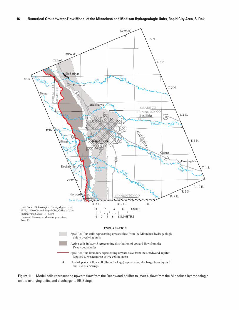
Figure 11. Model cells representing upward flow from the Deadwood aquifer to layer 4, flow from the Minnelusa hydrogeologic unit to overlying units, and discharge to Elk Spings.
MEADE CO
LAW
REN
CE
CO
PENNINGTON CO
MEA
DE
CO
PENNINGTON CO
CUSTER CO
Nemo
Caputa
Hisega
Hayward
Tilford
Piedmont
Box Elder
Blackhawk
Rockerville
Farmingdale
R. 8 E.
Elk
Boxelder
Rapid
Spring
Rapid City
Gulch
Creek
T. 5 N.
T. 3 N.
T. 4 N.
T. 1 S.
T. 2 N.
T. 1 N.
T. 2 S.
R. 6 E. R. 7 E.
R. 9 E.
R. 10 E.
103°07’30”
103°22’30”
43°55’
44°15’
44°05’
16
I-90
I-90
Creek
Creek
Creek
Creek
Base from U.S. Geological Survey digital data, 1977, 1:100,000, and Rapid City, Office of City Engineer map, 2005, 1:18,000 Universal Transverse Mercator projection, Zone 13
Victoria Creek
Deadm
an
Battle Creek
Little Elk
RockervilleGulch
Elk Springs
0 4 62 8 MILES
0 642 8 KILOMETERS
44
4479
79
Specified-flux cells representing upward flow from the Minnelusa hydrogeologic unit to overlying units
Active cells in layer 5 representing distribution of upward flow from the Deadwood aquifer
Specified-flux boundary representing upward flow from the Deadwood aquifer (applied to westernmost active cell in layer)
Head-dependent flow cell (Drain Package) representing discharge from layers 1 and 3 to Elk Springs
EXPLANATION
16 Numerical Groundwater-Flow Model of the Minnelusa and Madison Hydrogeologic Units, Rapid City Area, S. Dak.

Figure 12. Locations of head-dependent flow cells representing springs in the detailed study area.
44°05’
I-90
44
79
Rapid
16
Creek
Boxelder
Spring Creek
CreekMEADE CO
PENNINGTON CO
T. 1 N.
T. 1 S.
R. 7 E.
R. 6 E.
R. 5 E.
103°22’30”
103°15’
44°00’
T. 3 N.
T. 2 N.
Base fom U.S. Geological Survey digital data, 1977, 1:100,000 Rapid City, Office of City Engineer map, 2005, 1:18,000Unversal Transverse Mercator projectionZone 13 0 2 31 4 MILES
0 1 2 3 4 KILOMETERS
Rapid CityRapid City
79
44
16
Rapid
Creek
44032110318110106412900
Canyon Lake
City Springs
Jackson-Cleghorn Springs
Boxelder Springs
Infiltration Gallery Springs
Deadwood Avenue Springs
Canyon Lake
City Springs
Jackson-Cleghorn Springs
Infiltration Gallery Springs
Deadwood Avenue Springs
EXPLANATION
Head-dependent flow cell (Drain Package) representing discharge from model layer 1 to Boxelder and Infiltration Gallery Springs
Head-dependent flow cell (River Package) representing hydraulic connection of model layer 1 to Canyon Lake
Head-dependent flow cell (River Package) representing discharge from model layer 1 to Jackson-Cleghorn Springs
Head-dependent flow cell (Drain Package) representing discharge from model layer 3 to Jackson-Cleghorn Springs
Head-dependent flow cell (Drain Package) representing discharge from model layers 1 and 3 to City and Deadwood Avenue Springs
Streamflow-gaging station—Number is station identification
Numerical Groundwater-Flow Model 17

Table 1. Stress periods for transient simulations.
[Stress period identifiers: “W” represents the 6-month stress period from October through March, and “S” represents the 6-month period from April through October. Total recharge and water-use rates from Long and Putnam (2002)]
Stress period number
Stress period identifier
Time periodTotal recharge rate to Minnelusa and Madison hydrogeologic units
(cubic feet per second)
Water-use rate for Minnelusa and Madison hydrogeologic units
(cubic feet per second)
1 W–88 October 1, 1987–March 31, 1988 18.7 1.92 S–88 April 1, 1988–September 30, 1988 23.6 4.73 W–89 October 1, 1988–March 31, 1989 16.3 1.74 S–89 April 1, 1989–September 30, 1989 34.1 3.45 W–90 October 1, 1989–March 31, 1990 22.7 1.86 S–90 April 1, 1990–September 30, 1990 50.0 4.27 W–91 October 1, 1990–March 31, 1991 19.8 3.08 S–91 April 1, 1991–September 30, 1991 135.2 7.29 W–92 October 1, 1991–March 31, 1992 32.9 5.4
10 S–92 April 1, 1992–September 30, 1992 40.3 12.511 W–93 October 1, 1992–March 31, 1993 25.6 3.712 S–93 April 1, 1993–September 30, 1993 149.4 13.613 W–94 October 1, 1993–March 31, 1994 46.9 6.214 S–94 April 1, 1994–September 30, 1994 59.6 15.015 W–95 October 1, 1994– March 31, 1995 43.0 5.816 S–95 April 1, 1995–September 30, 1995 180.7 11.017 W–96 October 1, 1995–March 31, 1996 57.0 3.218 S–96 April 1, 1996–September 30, 1996 131.6 11.419 W–97 October 1, 1996–March 31, 1997 82.3 5.520 S–97 April 1, 1997–September 30, 1997 181.8 11.9
18 Numerical Groundwater-Flow Model of the Minnelusa and Madison Hydrogeologic Units, Rapid City Area, S. Dak.
to the observed data in inverse modeling or by trial-and-error methods were assigned fixed values that were considered to be within the range of values expected for the parameters. The following section describes the properties that were repre-sented with parameters and the remaining properties that were assigned values on the basis of previous estimates.
Representation of Flow-System Components
Flow-system components represented in the model include recharge, discharge, and hydraulic properties. Recharge includes streamflow recharge, areal recharge, and upward flow from the Deadwood aquifer. Upward flow from other underlying units was assumed to be small and included in upward flow represented in layer 5. Recharge to the hydrogeologic units occurs by two processes: streamflow recharge and areal recharge. Streamflow recharge originates from precipitation runoff in the central Black Hills upstream from the outcrops of the Minnelusa and Madison hydrogeo-logic units. These streams lose flow to swallow holes and fractures as they cross the outcrops. Areal recharge occurs
from infiltration of precipitation on the outcrops. Because of the fractures and openings on the outcrop, any precipita-tion that exceeds evapotranspiration is assumed to infiltrate. Discharge includes springflow, water use, flow to overlying units, and regional outflow. Hydraulic properties and model features include horizontal and vertical hydraulic conductivity, horizontal flow barriers, and storage properties.
A steady-state water budget (table 2) was estimated by modifying the water-balance analysis by Long and Putnam (2002). The water-balance analysis quantified budget compo-nents for twenty 6-month time steps for water years (WY) 1988–97 (table 1). The average water budget for that 10-year period included varied hydrologic conditions that collectively were assumed to approximate steady-state conditions. That water-balance analysis is described with more detail in the following subsections for each budget component.
Recharge and discharge were adjusted slightly to account for the change in storage that was included in the 10-year average water budget (1988–97) from Long and Putnam (2002). Inflow (recharge) was decreased by 4.4 ft3/s, and outflow was increased by 4.3 ft3/s to account for the change in storage of 8.7 ft3/s. Streamflow recharge was reduced by
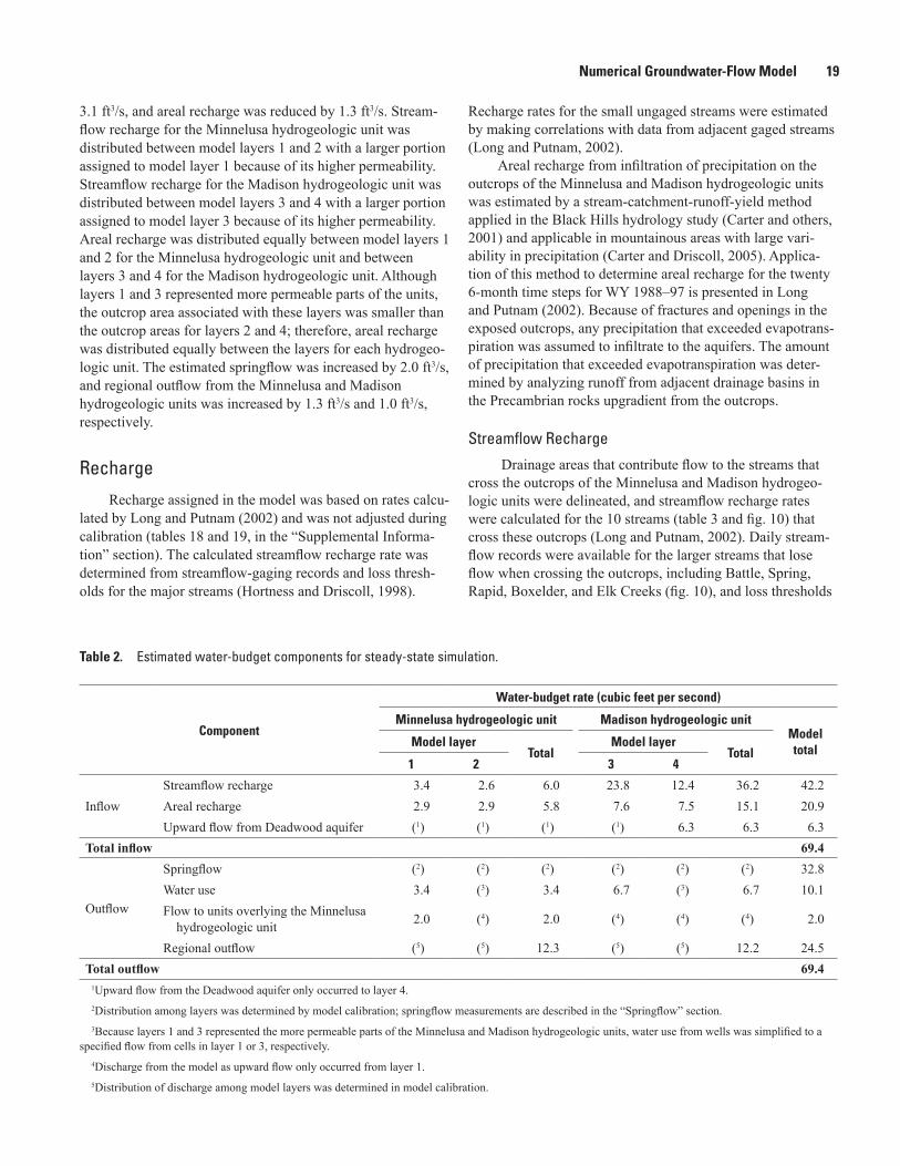
Table 2. Estimated water-budget components for steady-state simulation.
Component
Water-budget rate (cubic feet per second)
Minnelusa hydrogeologic unit Madison hydrogeologic unitModel total
Model layerTotal
Model layerTotal
1 2 3 4
InflowStreamflow recharge 3.4 2.6 6.0 23.8 12.4 36.2 42.2Areal recharge 2.9 2.9 5.8 7.6 7.5 15.1 20.9Upward flow from Deadwood aquifer (1) (1) (1) (1) 6.3 6.3 6.3
Total inflow 69.4
Outflow
Springflow (2) (2) (2) (2) (2) (2) 32.8Water use 3.4 (3) 3.4 6.7 (3) 6.7 10.1Flow to units overlying the Minnelusa
hydrogeologic unit 2.0 (4) 2.0 (4) (4) (4) 2.0
Regional outflow (5) (5) 12.3 (5) (5) 12.2 24.5Total outflow 69.4
1Upward flow from the Deadwood aquifer only occurred to layer 4.2Distribution among layers was determined by model calibration; springflow measurements are described in the “Springflow” section.3Because layers 1 and 3 represented the more permeable parts of the Minnelusa and Madison hydrogeologic units, water use from wells was simplified to a
specified flow from cells in layer 1 or 3, respectively.4Discharge from the model as upward flow only occurred from layer 1.5Distribution of discharge among model layers was determined in model calibration.
Numerical Groundwater-Flow Model 19
3.1 ft3/s, and areal recharge was reduced by 1.3 ft3/s. Stream-flow recharge for the Minnelusa hydrogeologic unit was distributed between model layers 1 and 2 with a larger portion assigned to model layer 1 because of its higher permeability. Streamflow recharge for the Madison hydrogeologic unit was distributed between model layers 3 and 4 with a larger portion assigned to model layer 3 because of its higher permeability. Areal recharge was distributed equally between model layers 1 and 2 for the Minnelusa hydrogeologic unit and between layers 3 and 4 for the Madison hydrogeologic unit. Although layers 1 and 3 represented more permeable parts of the units, the outcrop area associated with these layers was smaller than the outcrop areas for layers 2 and 4; therefore, areal recharge was distributed equally between the layers for each hydrogeo-logic unit. The estimated springflow was increased by 2.0 ft3/s, and regional outflow from the Minnelusa and Madison hydrogeologic units was increased by 1.3 ft3/s and 1.0 ft3/s, respectively.
Recharge
Recharge assigned in the model was based on rates calcu-lated by Long and Putnam (2002) and was not adjusted during calibration (tables 18 and 19, in the “Supplemental Informa-tion” section). The calculated streamflow recharge rate was determined from streamflow-gaging records and loss thresh-olds for the major streams (Hortness and Driscoll, 1998).
Recharge rates for the small ungaged streams were estimated by making correlations with data from adjacent gaged streams (Long and Putnam, 2002).
Areal recharge from infiltration of precipitation on the outcrops of the Minnelusa and Madison hydrogeologic units was estimated by a stream-catchment-runoff-yield method applied in the Black Hills hydrology study (Carter and others, 2001) and applicable in mountainous areas with large vari-ability in precipitation (Carter and Driscoll, 2005). Applica-tion of this method to determine areal recharge for the twenty 6-month time steps for WY 1988–97 is presented in Long and Putnam (2002). Because of fractures and openings in the exposed outcrops, any precipitation that exceeded evapotrans-piration was assumed to infiltrate to the aquifers. The amount of precipitation that exceeded evapotranspiration was deter-mined by analyzing runoff from adjacent drainage basins in the Precambrian rocks upgradient from the outcrops.
Streamflow Recharge
Drainage areas that contribute flow to the stream s that cross the outcrops of the Minnelusa and Madison hydrogeo-logic units were delineated, and streamflow recharge rates were calculated for the 10 streams (table 3 and fig. 10) that cross these outcrops (Long and Putnam, 2002). Daily stream-flow records were available for the larger streams that lose flow when crossing the outcrops, including Battle, Spring, Rapid, Boxelder, and Elk Creeks (fig. 10), and loss thresholds

Table 3. Steady-state streamflow recharge rates distributed by model layer.
Stream
Streamflow recharge rate (cubic feet per second)
Minnelusa hydrogeologic unit Madison hydrogeologic unit Total
modelModel layer
Total Model layer
Total 1 2 3 4
Elk Creek 0.4 0.4 0.8 1.2 1.2 2.4 3.2Little Elk Creek .3 .3 .6 .3 .3 .6 1.2Boxelder Creek 1.4 .6 2.0 9.1 2.8 11.9 13.9Unnamed tributary on Rapid Creek .0 .0 .0 .1 .1 .2 .2Rapid Creek .9 .9 1.8 4.5 3.0 7.5 9.3Victoria Gulch (1) (1) (1) (1) .8 .8 .8Spring Creek .4 .4 .8 6.9 2.3 9.2 10.0Rockerville Gulch .0 .0 .0 .4 .4 .8 .8Deadman Gulch .0 .0 .0 .0 .2 .2 .2Battle Creek (2) (2) (2) 1.3 1.3 2.6 2.6Total 3.4 2.6 6.0 23.8 12.4 36.2 42.2
1The stream did not cross the part of the hydrogeologic unit represented by layers 1, 2, or 3.2Streamflow loss was offset by reemerging springs.
20 Numerical Groundwater-Flow Model of the Minnelusa and Madison Hydrogeologic Units, Rapid City Area, S. Dak.
for all but 2 of the 10 streams were deter mined by Hortness and Driscoll (1998). For the other two streams (Rockerville Gulch and Deadman Gulch), loss thresholds were estimated by Long and Putnam (2002). For the small ungaged streams, flow was estimated by correlation with flow at adjacent gaged streams as described in Long and Putnam (2002), and the distribution of recharge among the model layers was approxi-mated. Measured or estimated daily streamflow less than or equal to the loss threshold recharged the Madison hydro-geologic unit, and once that threshold flow was exceeded, streamflow recharged the Minnelusa hydrogeologic unit at a rate equal to the loss threshold for this unit.
Streamflow recharge was represented with specified-flow cells (Well Package, McDonald and Harbaugh, 1998) in model layers 1–4 (fig. 10). The recharge was distributed between the four layers with larger amounts assigned to layers 1 and 3, which represented the more permeable parts of each hydrogeologic unit. Streamflow recharge rates assigned to the steady-state simulation (table 3) show the relatively large contributions from Boxelder, Rapid, and Spring Creeks. Because Battle Creek and Elk Creek were on the southern and northern boundaries of the model, respectively, it was assumed that one-half of the streamflow recharge for these streams entered the model area. When streamflow was adequate to flow through the loss zones, the more permeable layers 1 and 3 were assigned a larger portion of the recharge calculated for each hydrogeologic unit. When streamflow was less than the loss threshold, layer 4 had the first opportunity to receive recharge; therefore, for stress periods with relatively small streamflow, the recharge to layers 3 and 4 was about equal. As streamflow increased, layer 4 could not accept any more
recharge and layer 3 received the increase in streamflow. A similar scenario occurred for layers 1 and 2; however, avail-able flow was reduced by the upstream loss to layers 3 and 4. Spring Creek and Boxelder Creek had the largest streamflow loss thresholds; thus, the largest streamflow recharge to layer 3 occurred along these two streams. Rapid Creek almost always exceeded the loss threshold because streamflow was regulated by releases from an upstream dam; therefore, the distribution of streamflow recharge for this stream was the same for all stress periods.
Transient streamflow recharge rates for the Minnelusa and Madison hydrogeologic units are presented in table 18 in the “Supplemental Information” section for each of the 10 streams. Total transient streamflow recharge rates for all streams by stress period for the Minnelusa and Madison hydrogeologic units ranged from 14.1 ft3/s (stress period 3, winter WY 1989) to 102.2 ft3/s (stress period 20, summer WY 1997). Distribution of transient streamflow recharge rates for 20 stress periods by model layer (fig. 13) shows the rela-tively large rates during wet periods (stress periods 12–20). Because the Minnelusa hydrogeologic unit receives recharge only when streamflow exceeds the loss threshold for the Madison hydrogeologic unit, streamflow recharge rates to model layers 1 and 2 were substantially less than streamflow recharge rates to model layers 3 and 4.
Areal Recharge
The methods used for calculating the areal recharge are described in detail in Long and Putnam (2002) and summa-rized here. The outcrop area of the Minnelusa and Madison

Figure 13. Total transient streamflow recharge rates for twenty 6-month stress periods by model layer.
0
20
40
60
80
100
120
1 2 3 4 5 6 7 8 9 10 11 12 13 14 15 16 17 18 19 20
STRE
AMFL
OW R
ECHA
RGE
RATE
, IN
CUB
IC F
EET
PER
SECO
ND
TRANSIENT 6-MONTH STRESS PERIODS FOR WATER YEARS 1988−97
Layer 1Layer 2Layer 3Layer 4
Table 4. Areal recharge zones and average annual precipitation on outcrops of the Minnelusa and Madison hydrogeologic units.
[From Long and Putnam (2002). Outcrop zone represents extent of hydrogeologic unit outcrop bounded by streams crossing the outcrop. Average annual pre-cipitation by hydrogeologic unit was calculated from precipitation data for water years 1961–98 by Driscoll, Hamade, and Kenner (2000). NA, not applicable]
Outcrop zone
Outcrop zone number
shown on fig. 14
Outcrop area by hydrogeologic unit
(square miles)
Average annual precipitation by
hydrogeologic unit(inches)
Average annual precipitation rate by hydrogeologic unit
(cubic feet per second)
Minnelusa Madison Minnelusa Madison Minnelusa Madison
Elk Creek to Little Elk Creek 1 3.6 10.1 22.3 24.0 5.9 17.9
Little Elk Creek to Boxelder Creek 2 15.2 27.3 19.2 20.0 21.5 40.2
Boxelder Creek to Rapid Creek 3 12.5 9.8 18.9 19.6 17.4 14.2
Rapid Creek to Spring Creek 4 7.1 4.6 18.6 19.1 9.7 6.5
Spring Creek to Battle Creek 5 15.1 6.6 19.4 19.9 21.6 9.7
Total NA 53.5 58.4 NA NA 76.1 88.5
Numerical Groundwater-Flow Model 21
hydrogeologic units was subdivided into five zones for calculation of areal recharge from infiltration of precipitation on the outcrops (table 4 and fig. 14). The zones represented infiltration of precipitation on the outcrop areas between major streams. The fraction of precipitation that was available for recharge after evapotranspiration was represented by runoff in gaged stream basins in Precambrian rocks adjacent to the outcrop areas. Most of the groundwater infiltration in these Precambrian basins with high relief returns to the basins as springflow; therefore, the runoff per unit area was assumed to represent the fraction of precipitation that was available for infiltration on the adjacent outcrops.
The areal recharge was distributed equally between the two model layers representing each hydrogeologic unit. The distribution was assumed to be equal because the more permeable layers 1 and 3 represented a smaller percentage of the total outcrop area than the thicker layers 2 and 4. The recharge flux for each model layer was assigned to the first downgradient (westernmost) active model cell. Steady-state areal recharge by zone and model layer (table 5) shows larger recharge rates for the northern zones because of greater precip-itation and larger outcrop areas for these zones than for the southern zones. Calculated areal recharge rates for the Minn-elusa hydrogeologic unit were less than rates for the Madison

Figure 14. Locations of areal recharge zones.
MEADE CO
PENNINGTON CO
PENNINGTON CO
CUSTER CO
Nemo
Caputa
Hisega
Hayward
Tilford
Piedmont
Box Elder
Blackhawk
Rockerville
Farmingdale
R. 8 E.
Elk
Boxelder
Rapid
Spring
Rapid City
Gulch
Creek
T. 5 N.
T. 3 N.
T. 4 N.
T. 1 S.
T. 2 N.
T. 1 N.
T. 2 S.
R. 6 E. R. 7 E.
R. 9 E.
R. 10 E.
103°07’30”
103°22’30”
43°55’
44°15’
44°05’
16
I-90
I-90
Creek
Creek
Creek
Creek
EXPLANATION
Base from U.S. Geological Survey digital data, 1977, 1:100,000, and Rapid City, Office of City Engineer map, 2005, 1:18,000 Universal Transverse Mercator projection, Zone 13
Victoria Creek
Deadm
an
Battle Creek
Little Elk
RockervilleGulch
79
0 4 62 8 MILES
0 642 8 KILOMETERS
4479
44
Outcrop of Minnelusa hydrogeologic unit
Outcrop of Madison hydrogeologic unit
1
2
3
4
5
Areal recharge zone (tables 5 and 19)
Geologic outcrops modified from Strobel and others, 1999
22 Numerical Groundwater-Flow Model of the Minnelusa and Madison Hydrogeologic Units, Rapid City Area, S. Dak.

Table 5. Areal recharge zones and steady-state areal recharge rates distributed by model layer.
[Outcrop zone represents extent of hydrogeologic unit outcrop bounded by streams crossing the outcrop. NA, not applicable]
Outcrop zone
Outcrop zone number
shown on fig. 14
Areal recharge rate (cubic feet per second)
Minnelusa hydrogeologic unit Madison hydrogeologic unitTotal
modelModel layer
TotalModel layer
Total1 2 3 4
Elk Creek to Little Elk Creek 1 0.3 0.3 0.6 1.6 1.6 3.2 3.8Little Elk Creek to Boxelder Creek 2 1.1 1.1 2.2 3.8 3.7 7.5 9.7Boxelder Creek to Rapid Creek 3 .6 .6 1.2 1.2 1.2 2.4 3.6Rapid Creek to Spring Creek 4 .2 .2 .4 .4 .4 .8 1.2Spring Creek to Battle Creek 5 .7 .7 1.4 .6 .6 1.2 2.6Total NA 2.9 2.9 5.8 7.6 7.5 15.1 20.9
Numerical Groundwater-Flow Model 23
hydrogeologic unit because 50 percent of the precipitation that fell on the thin western part of the Minnelusa hydrogeologic unit outcrop was assumed to have infiltrated downward to the Madison hydrogeologic unit.
Transient areal recharge rates for the Minnelusa and Madison hydrogeologic units (Long and Putnam, 2002) are presented in table 19 in the “Supplemental Information” section. Total transient areal recharge by stress period (fig. 15) shows the substantially larger areal recharge during wet stress periods (stress periods 12–20) compared to recharge during dry periods (stress periods 1–11). During the stress periods with large precipitation, a greater fraction of precipitation becomes recharge. During the summer stress periods 8, 12, 16, and 20, areal recharge was about the same as streamflow recharge (fig. 13); however, during the winter stress periods and drier summer stress periods, streamflow recharge was larger than areal recharge. Total transient areal recharge rates by stress period for the Minnelusa and Madison hydrogeologic units (table 19) ranged from 1.1 ft3/s (stress period 1, winter WY 1988) to 98.4 ft3/s (stress period 16, summer WY 1995). Most of the steady-state areal recharge occurred during the wet summer periods. The steady-state areal recharge rate (table 5) was largest for the Little Elk Creek to Boxelder Creek zone (zone 2) because of the relatively large outcrop area and greater precipitation in this zone than in the southern zones.
Upward Flow from Deadwood Aquifer
Layer 5 represented an approximation of the underlying Deadwood aquifer to simulate upward flow to the Madison hydrogeologic unit. The average upward flow from the Dead-wood aquifer to the Madison hydrogeologic unit was esti-mated by Long and Putnam (2002) to be 6.3 ft3/s in the study area, representing about 9 percent of the total average inflow to the model. This upward flow was assumed to be constant during transient simulations. Although the hydraulic head in the Deadwood aquifer and the Madison hydrogeologic unit
changed over time, it was assumed that the vertical gradient between the two units did not change substantially. Input to model layer 5 was accomplished by a specified flux (fig. 11) equally distributed to the westernmost cells in layer 5.
DischargeSpringflow, water use, flow to overlying units, and
regional outflow were estimated by Long and Putnam (2002). Water use was assigned to the model by using specified-flow cells. Flow to overlying units was assumed to be small and assigned a value that did not change in transient simulations. Simulated springflow and regional outflow rates were depen-dent on the conductance of head-dependent cells, which was estimated by model calibration.
Springflow
Discharge from springs (figs. 11 and 12) calculated by model simulation was the difference between the user-specified hydraulic head of the spring and the simulated hydraulic head multiplied by the conductance for the cell. Conductance is a term that groups the hydraulic conductiv-ity and the length of flow path. The conductance term for springs was represented as a parameter that was adjusted in model calibration (described in the subsequent “Steady-State Calibration” section and “Transient Calibration” section) to produce the best fit with estimated flows and hydraulic head values. Generally, the Madison hydrogeologic unit has been interpreted as the major source of water for large springs in the model area on the basis of hydrochemistry and the presence of conduits (Anderson and others, 1999; Long and Putnam, 2002). Although the Madison hydrogeologic unit is the predominant source of water for the springs, substantial interaction between the upward flow and the Minnelusa hydro-geologic unit is possible. In representing discharge from these springs, both the Minnelusa and Madison hydrogeologic units

Figure 15. Total transient areal recharge rates for twenty 6-month stress periods by model layer and spatially averaged precipitation on outcrops of the Minnelusa and Madison hydrogeologic units.
0
5
10
15
20
25
0
20
40
60
80
100
120
1 2 3 4 5 6 7 8 9 10 11 12 13 14 15 16 17 18 19 20
SPAT
IALL
Y AV
ERAG
ED P
RECI
PITA
TION
, IN
INCH
ES
AREA
L R
ECHA
RGE
RATE
, IN
CUB
IC F
EET
PER
SECO
ND
TRANSIENT 6-MONTH STRESS PERIODS FOR WATER YEARS 1988−97
Recharge rate to layer 1Recharge rate to layer 2Recharge rate to layer 3Recharge rate to layer 4Precipitation
24 Numerical Groundwater-Flow Model of the Minnelusa and Madison Hydrogeologic Units, Rapid City Area, S. Dak.
were considered as potential sources. Steady-state springflow (table 6) was estimated by Anderson and others (1999) and Long and Putnam (2002).
The springflow of Jackson-Cleghorn Springs, the largest spring in the study area, was estimated as 21.6 ft3/s by a water-budget analysis of a Rapid Creek stream reach that extended through the Jackson-Cleghorn complex (Anderson and others, 1999). On the basis of stable isotope data, they concluded that the springs were a regional discharge point from the Madison aquifer. The spring’s discharge from the Madison hydrogeologic unit in the current model was represented with two head-dependent flow cells (Drain Package, McDonald and Harbaugh, 1998) in layer 3 (fig. 12) with hydraulic head set equal to the hydraulic head in the alluvium (Anderson and others, 1999), and the conductance was represented with parameter CLEGmdsn that was estimated in model calibra-tion. Although assumed to be small, a contribution to spring discharge from the Minnelusa hydrogeologic unit also is possible. The component of discharge from Jackson-Cleghorn Springs from the Minnelusa hydrogeologic unit was repre-sented with five head-dependent cells in layer 1 located along the Rapid Creek reach near Jackson-Cleghorn Springs (fig. 12). This hydraulic connection was represented with special head-dependent flow cells (River Package, McDonald and Harbaugh, 1998) that allowed both outflow and inflow
to the model depending on the relation between the hydrau-lic head of the water body and the hydraulic head in the cell. Conductance was represented with parameter CLEGmnls that was estimated in calibration. This Rapid Creek stream reach and associated alluvium overlies the outcrop of the Minn-elusa hydrogeologic unit and was assumed to be hydraulically connected to the unit.
Comparison of hydraulic head values in the Minn-elusa and Madison hydrogeologic units and Rapid Creek at Jackson Springs, located in the southwest part of the Jackson-Cleghorn springs area provides some insight on the potential for interaction between the Minnelusa and Madison hydro-geologic units. On September 8, 1999, hydraulic head in the Minnelusa hydrogeologic unit in the observation well at site 231 (well JS–1B; table 20 in “Supplemental Information” section), which is located near Jackson-Cleghorn Springs, was about 17 ft above Rapid Creek. At site 52, a nested well completed in the Madison hydrogeologic unit (well JS–1A; table 21 in “Supplemental Information” section), hydraulic head was about 40 ft above Rapid Creek. Hydraulic head in the Minnelusa hydrogeologic unit was about 10 ft higher at site 231 than it was in the observation well at site 233 (well CHLN–1; table 20), which is located about 0.5 mi south of site 231. This higher hydraulic head indicted the possibility of a mound created in the Minnelusa hydrogeologic unit from

Table 6. Steady-state springflow.
[NA, not applicable]
Spring nameConductance parameter
namesSteady-state springflow (cubic feet per second)
Jackson-Cleghorn Springs CLEGmdsn, CLEGmnls 121.6City Springs CITYSPR 21.7Deadwood Avenue Springs DWSPR 22.8Boxelder Springs BESPR 21.0Elk Springs ELKSPR 23.7Infiltration Gallery Springs GAL 11.5Canyon Lake CLAKE 3.5Total NA 32.8
1From Anderson and others, 1999.2From Long and Putnam, 2002.3No quantitative measurements were available; small discharge was assumed because of hydraulic
connection.
Numerical Groundwater-Flow Model 25
water moving upward from the Madison hydrogeologic unit. The vertical hydraulic conductivity for cells in layer 2 in the Jackson-Cleghorn Springs area was assumed to be substan-tially higher than surrounding areas because of collapse features and solution enhanced openings. The multiplier for layer 2 vertical hydraulic conductivity was determined in model calibration.
Discharge at City Springs was represented by head-dependent cells (Drain Package, McDonald and Harbaugh, 1998) in layers 1 and 3 (fig. 12), and the conductance was assumed to be similar for the two cells and was represented with parameter CITYSPR. Because of the structural features in this area (fig. 1), vertical hydraulic conductivity for layer 2 in the City Springs area was assumed to be substantially higher than for other parts of layer 2. During dry periods, flow from this spring decreased to near zero (Long and Putnam, 2002).
Discharge at Deadwood Avenue Springs was represented with head-dependent cells (Drain Package, McDonald and Harbaugh, 1998) in both layers 1 and 3 (fig. 12). In the Dead-wood Avenue Springs area, the average hydraulic head (Long and Putnam, 2002) was about 100 ft above the land surface in the Madison hydrogeologic unit and near the land surface in the Minnelusa hydrogeologic unit. Therefore, most spring discharge probably occurred from the Madison hydrogeologic unit. Conductance was assumed similar for both cells and was estimated with parameter DWSPR in model calibration.
Boxelder Springs was assumed to increase from no flow in dry periods to estimated flows of about 7 ft3/s in wet periods (Carter and others, 2001; Long and Putnam, 2002). Because the hydraulic head in the Madison hydrogeologic unit was always well above the land surface even during periods when there was no observed spring discharge, Boxelder Springs was assumed to discharge from the Minnelusa hydrogeologic
unit and was represented with a head-dependent cell (Drain Package, McDonald and Harbaugh, 1998) in layer 1 (fig. 12), and conductance was estimated with parameter BESPR in model calibration.
Elk Springs was represented by five head-dependent cells (Drain Package, McDonald and Harbaugh, 1998) in both layers 1 and 3 (fig. 11) upstream on Elk Creek from the point identified as the spring on the map in Long and Putnam (2002). During the wet periods (late 1990s), flow was observed to increase in the downstream direction in this reach. Flow was very low during the dry periods, but increased dramatically during the wet periods. On the basis of hydraulic head values, the source potentially could be both the Minn-elusa and Madison hydrogeologic units. Conductance was assumed to be similar for each layer and was estimated with parameter ELKSPR in model calibration.
Anderson and others (1999) estimated a small discharge contribution of about 1.5 ft3/s from bedrock units to two infiltration galleries along Rapid Creek about 0.7 mi and 1.2 mi downstream, respectively, from Canyon Lake. This discharge was represented by two head-dependent cells (Drain Package, McDonald and Harbaugh, 1998) in layer 1 (fig. 12), and conductance was estimated with parameter GAL in model calibration.
When Canyon Lake was drained in the winter of 1995–96, hydraulic head in an observation well completed in the Minnelusa hydrogeologic unit near Canyon Lake (site 229, table 20) responded with a similar decline in hydraulic head (Driscoll, Bradford, and Moran, 2000). Canyon Lake was represented with six head-dependent cells (River Package, McDonald and Harbaugh, 1998) in layer 1 (fig. 12) that allowed inflow or outflow from the model depending on the hydraulic head relation, and conductance was estimated with parameter CLAKE in model calibration.

Table 7. Water-use rates for steady-state and transient simulations.
[From Long and Putnam (2002). W, winter; S, summer (W–88 = winter, water year 1988)]
Stress period
Other stress period
identifier
Water-use rate (cubic feet per second)
Model layer 1 (Minnelusa hydrogeologic unit)
Model layer 3 (Madison hydrogeologic unit)
Total model
Rapid City
Other domestic
and public water
supplies
Industrial and
irrigation use
Totallayer 1
Rapid City
Other domestic
and public water
supplies
Industrial and
irrigation use
Total layer 3
1 W–88 1.5 1.2 0.2 2.9 0.0 1.3 0.6 1.9 4.8
2 S–88 1.4 3.1 1.2 5.7 .0 3.4 1.3 4.7 10.4
3 W–89 .5 1.0 .2 1.7 .0 1.1 .6 1.7 3.4
4 S–89 .7 1.8 1.2 3.7 .1 2.0 1.3 3.4 7.1
5 W–90 1.6 1.1 .2 2.9 .0 1.2 .6 1.8 4.7
6 S–90 1.9 1.8 1.2 4.9 .9 2.0 1.3 4.2 9.1
7 W–91 1.8 1.3 .2 3.3 1.0 1.4 .6 3.0 6.3
8 S–91 1.6 2.0 1.0 4.6 3.3 2.2 1.7 7.2 11.8
9 W–92 1.3 1.1 .2 2.6 3.6 1.2 .6 5.4 8.0
10 S–92 1.2 1.9 1.2 4.3 9.1 2.1 1.3 12.5 16.8
11 W–93 1.1 1.3 .2 2.6 1.7 1.4 .6 3.7 6.3
12 S–93 1.1 1.8 1.1 4.0 10.6 1.9 1.1 13.6 17.6
13 W–94 .6 1.3 .2 2.1 4.2 1.4 .6 6.2 8.3
14 S–94 .3 2.6 1.2 4.1 10.9 2.8 1.3 15.0 19.1
15 W–95 .8 1.3 .2 2.3 3.7 1.4 .7 5.8 8.1
16 S–95 .6 2.1 1.0 3.7 7.5 2.3 1.2 11.0 14.7
17 W–96 .5 1.4 .2 2.1 .9 1.6 .7 3.2 5.3
18 S–96 .6 2.4 1.0 4.0 7.6 2.6 1.2 11.4 15.4
19 W–97 .8 1.5 .2 2.5 3.2 1.6 .7 5.5 8.0
20 S–97 .9 2.2 1.0 4.1 8.4 2.3 1.2 11.9 16.0Average (steady state) 1.0 1.7 .7 3.4 3.8 1.9 1.0 6.7 10.1
26 Numerical Groundwater-Flow Model of the Minnelusa and Madison Hydrogeologic Units, Rapid City Area, S. Dak.
Water UseWater-use estimates (table 7) from Long and Putnam
(2002) were used in model simulations. All water use was represented by specified-flow cells (Well Package, McDonald and Harbaugh, 1998) in layer 1 for pumping in the Minnelusa hydrogeologic unit and in layer 3 for pumping in the Madison hydrogeologic unit (fig. 16). The average water-use rates for the Minnelusa and Madison hydrogeologic units for the 10-year period were 3.4 and 6.7 ft3/s, respectively. The average combined pumping rates were 6.3 ft3/s for the October–March (W) stress periods and 13.8 ft3/s for the April–September (S) stress periods. The highest average pumping rate of 19.1 ft3/s was for stress period 14 (S–94).
Flow to Overlying UnitsGroundwater under confined pressure in the Minnelusa
hydrogeologic unit probably flows into overlying units (figs. 2 and 3) including aquifers in the Minnekahta Limestone and Inyan Kara Group through frac tures or breccia pipes. Because very little information was available to calculate the upward flow from the Minnelusa hydrogeologic unit, the estimate of 2.0 ft3/s from the water-budget calculation in Long and Putnam (2002) was uniformly assigned to the specified-flux cells (Recharge Package, McDonald and Harbaugh, 1998; fig. 11). Evidence supporting the potential upward flow is presented in Long and Putnam (2002).

Figure 16. Locations of specified-flow cells representing water use in model layers 1 and 3.
MEADE CO
LAW
REN
CE
CO
PENNINGTON CO
MEA
DE
CO
PENNINGTON CO
CUSTER CO
Nemo
Caputa
Hisega
Hayward
Tilford
Piedmont
Box Elder
Blackhawk
Rockerville
Farmingdale
R. 8 E.
Elk
Boxelder
Rapid
Spring
Rapid CityGulch
Creek
T. 5 N.
T. 3 N.
T. 4 N.
T. 1 S.
T. 2 N.
T. 1 N.
T. 2 S.
R. 6 E. R. 7 E.
R. 9 E.
R. 10 E.
103°07’30”
103°22’30”
43°55’
44°15’
44°05’
16
I-90
I-90
Creek
Creek
Creek
Base from U.S. Geological Survey digital data, 1977, 1:100,000, and Rapid City, Office of City Engineer map, 2005, 1:18,000 Universal Transverse Mercator projection, Zone 13
Victoria Creek
Deadm
an
Battle Creek
Little Elk
RockervilleGulch
79
Creek
0 4 62 8 MILES
0 642 8 KILOMETERS
44
44
79
Specified-flow cell representing production wells in layer 1
Specified-flow cell representing production wells in layer 3
Geologic outcrops modified from Strobel and others, 1999
EXPLANATION
Outcrop of Minnelusa hydrogeologic unit
Outcrop of Madison hydrogeologic unit
Numerical Groundwater-Flow Model 27

28 Numerical Groundwater-Flow Model of the Minnelusa and Madison Hydrogeologic Units, Rapid City Area, S. Dak.
Regional Outflow
Regional outflow to the east was estimated by Long and Putnam (2002) to be 22.2 ft3/s. The model boundary was extended about 6 mi farther east than the eastern boundary used to define the aquifer analysis area in Long and Putnam (2002) to minimize the effect of the boundary on the detailed study area. Head-dependent flow cells (Drain Package, McDonald and Harbaugh, 1998) represented the boundary (figs. 8 and 9) with the hydraulic head extrapolated from Long and Putnam (2002). Conductance for head-dependent cells in layers 1 and 2 at the eastern boundary was represented with parameter MnlsEB, and conductance for head-dependent cells in layers 3 and 4 was represented with parameter MdsnEB. Steady-state discharge was estimated as 12.3 ft3/s from the Minnelusa hydrogeologic unit and 12.2 ft3/s from the Madison hydrogeologic unit.
Hydraulic Properties
Hydraulic properties represented include horizontal hydraulic conductivity, vertical hydraulic conductivity, conductance of horizontal flow barriers, and storage coef-ficients. Hydraulic properties were represented by parameters that included cells grouped into zones.
Horizontal Hydraulic Conductivity
Horizontal hydraulic conductivity values for active cells in layer 1 were estimated by using three parameters named HK1_1, HK1_2, and HK1_3 (fig. 17) and multiplier arrays. Parameter group HK1_1 represented zones where the relatively gradual hydraulic gradient is attributable to larger hydraulic conductivity. Parameter group HK1_3 represented a zone where the relatively steep hydraulic gradient indicated potentially lower hydraulic conductivity. Parameter group HK1_2 represented a zone where the hydraulic conductivity was assumed to be between the values in zones HK1_1 and HK1_3. Areas near streamflow loss zones included subzones with large hydraulic conductivity that were assigned values by using a multiplier of five times the hydraulic conductivity in each respective zone. These small areas are near streams with substantial streamflow recharge where solution and collapse features cause increased permeability.
Hydraulic conductivity for layer 2 was represented as the product of the hydraulic conductivity of layer 1 times a multi-plier. The multiplier was set as 0.1 for most of the active cells in layer 2. The multiplier for active cells in layer 2 near the western boundary was set as 0.5 (fig. 18); this higher multi-plier accounted for the enhanced permeability in layer 2 near the outcrop area of the Minnelusa hydrogeologic unit resulting from fracturing, weathering, and dissolution.
Hydraulic properties for active cells in layer 3 were repre-sented with seven parameters named HK3_1, HK3_2, HK3_3, HK3_4, and HK3_5, HK3_6, and HK3_7 (fig. 19). Most of the discharge from Jackson-Cleghorn Springs represents a
regional discharge point from the Madison hydrogeologic unit (Anderson and others, 1999), and substantially enlarged solution openings probably exist in the vicinity of the spring. The zone surrounding Jackson-Cleghorn Springs (fig. 19) was grouped in parameter HK3_6. Parameter group HK3_7 repre-sented a zone of large hydraulic conductivity in the general areas of conduit flow paths from Spring Creek (Putnam and Long, 2007; Long and others, 2008) and the area surround-ing zone HK3_6. Parameter group HK3_4 represented the western area of Boxelder Creek that had a relatively gradual hydraulic gradient. Parameter group HK3_5 represented the areas near the outcrop that were assumed to have lower hydraulic conductivity than the areas near streams. Parameter group HK3_5 also represented other areas where the hydraulic gradient transitioned from gradual to steep. Parameter group HK3_3 represented an area where the hydraulic gradient was much steeper than for the surrounding areas and hydraulic conductivity was assumed to be substantially lower. Parameter group HK3_1 represented a high transmissivity zone described by Downey (1986). The horizontal hydraulic conductivity for the parameter group HK3_1 area included anisotropy repre-sented by parameter HANI3_2. The hydraulic conductivity for parameter group HK3_1 was greater in the direction of model rows than in the direction of model columns. Parameter group HK3_2 represented the remaining areas that had relatively gradual hydraulic gradients.
Additional information was available to characterize hydraulic conductivity in the detailed study area (fig. 20). Wells completed in the Madison hydrogeologic unit that were used as the basis for the characterization are listed in table 8. Hydraulic conductivity parameter groups HK3_4, HK3_6, and HK3_7 in model layer 3 represented areas that probably include substantial solution enlargement. Parameter group HK3_4 included wells 32, 35, 36, and 40 (fig. 20) where dye was detected following injection of dye in Boxelder Creek (Greene, 1999). The relatively large recharge from Boxelder Creek and the dispersed detection of dye indicated the likeli-hood of a relatively large hydraulic conductivity. This zone also contains structural features that could have contributed to enlargement of solution openings in the Madison hydrogeo-logic unit. A small area south of this zone that includes well 44 was represented with parameter group HK3_5 because of a steep hydraulic gradient in the area. The difference in hydrau-lic head between wells 40 and 44, which are about 2,000 ft apart, was about 100 ft (table 21).
Parameter group HK3_7 represented an area that was assumed to have relatively high hydraulic conductivity because of preferential flow paths, structural features, and relatively gradual hydraulic gradient. The parameter zone includes a potential flow path from the Spring Creek loss zone towards Jackson-Cleghorn Springs. Dye injected in Spring Creek was detected at sites CRO, NON, 66 (HH), and NAY (Putnam and Long, 2007). Analysis of a time-series of oxygen isotope values for Spring Creek streamflow recharge and water samples from site 71 (HR–2), also indicated a potential flow path from Spring Creek toward site 71 (Long and Putnam,

Figure 17. Horizontal hydraulic conductivity parameter groups and zones for model layer 1.
MEADE CO
LAW
REN
CE
CO
PENNINGTON CO
MEA
DE
CO
PENNINGTON CO
CUSTER CO
Nemo
Caputa
Hisega
Hayward
Tilford
Piedmont
Box Elder
Blackhawk
Rockerville
Farmingdale
R. 8 E.
Elk
Boxelder
RapidSpring
Rapid CityGulch
Creek
T. 5 N.
T. 3 N.
T. 4 N.
T. 1 S.
T. 2 N.
T. 1 N.
T. 2 S.
R. 6 E. R. 7 E.
R. 9 E.
R. 10 E.
103°07’30”
103°22’30”
43°55’
44°15’
44°05’
16
I-90
I-90
Creek
Creek
Creek
Creek
EXPLANATION
Base from U.S. Geological Survey digital data, 1977, 1:100,000, and Rapid City, Office of City Engineer map, 2005, 1:18,000 Universal Transverse Mercator projection, Zone 13
Victoria Creek
Deadm
an
Battle Creek
Little Elk
RockervilleGulch
79
44
4479
3,200
3,100
3,300
3,400
3,000
2,900
2,80
0
2,70
0
3,50
0
2,60
0
3,70
03,
600
3,80
0
3,600
3,50
0
3,50
0
3,40
0
3,000
2,900
2,800
3,1003,200
3,300
Horizontal hydraulic conductivity parameter groups and zonesHK1_1
HK1_2
HK1_3
Hydraulic conductivity multiplier zone within parameter groups representing areas near streamflow loss zones (multiplier of 5)
Minnelusa aquifer potentiometric contour (average for water years 1988–97; Long and Putnam, 2002)—Contour interval 100 feet. Datum is National Geodetic Vertical Datum of 1929
3,400
0 4 62 8 MILES
0 642 8 KILOMETERS
Numerical Groundwater-Flow Model 29
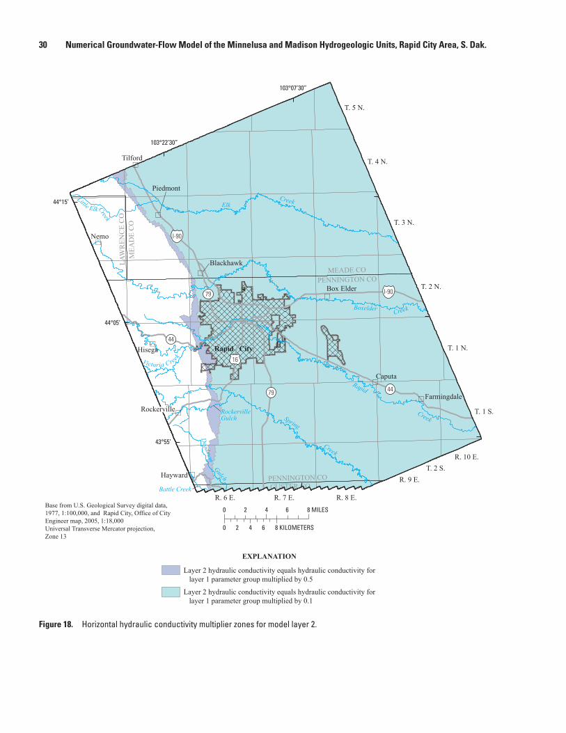
MEADE CO
LAW
REN
CE
CO
PENNINGTON CO
MEA
DE
CO
PENNINGTON CO
CUSTER CO
Nemo
Caputa
Hisega
Hayward
Tilford
Piedmont
Box Elder
Blackhawk
Rockerville
Farmingdale
R. 8 E.
Elk
Boxelder
Rapid
Spring
Rapid CityGulch
Creek
T. 5 N.
T. 3 N.
T. 4 N.
T. 1 S.
T. 2 N.
T. 1 N.
T. 2 S.
R. 6 E. R. 7 E.
R. 9 E.
R. 10 E.
103°07’30”
103°22’30”
43°55’
44°15’
44°05’
16
I-90
I-90
Creek
Creek
Creek
Creek
EXPLANATION
Base from U.S. Geological Survey digital data, 1977, 1:100,000, and Rapid City, Office of City Engineer map, 2005, 1:18,000 Universal Transverse Mercator projection, Zone 13
Victoria Creek
Deadm
an
Battle Creek
Little Elk
RockervilleGulch
79
0 4 62 8 MILES
0 642 8 KILOMETERS
44
4479
Layer 2 hydraulic conductivity equals hydraulic conductivity for layer 1 parameter group multiplied by 0.5
Layer 2 hydraulic conductivity equals hydraulic conductivity for layer 1 parameter group multiplied by 0.1
Figure 18. Horizontal hydraulic conductivity multiplier zones for model layer 2.
30 Numerical Groundwater-Flow Model of the Minnelusa and Madison Hydrogeologic Units, Rapid City Area, S. Dak.

MEADE CO
LAW
REN
CE
CO
PENNINGTON CO
MEA
DE
CO
PENNINGTON CO
CUSTER CO
Nemo
Caputa
Hisega
Hayward
Tilford
Piedmont
Box Elder
Blackhawk
Rockerville
Farmingdale
R. 8 E.
Elk
Boxelder
Rapid
Spring
RapidCity
Gulch
Creek
T. 5 N.
T. 3 N.
T. 4 N.
T. 1 S.
T. 2 N.
T. 1 N.
T. 2 S.
R. 6 E. R. 7 E.
R. 9 E.
R. 10 E.
103°07’30”
103°22’30”
43°55’
44°15’
44°05’
16
I-90
I-90
Creek
Creek
Creek
Creek
EXPLANATION
Base from U.S. Geological Survey digital data, 1977, 1:100,000, and Rapid City, Office of City Engineer map, 2005, 1:18,000 Universal Transverse Mercator projection, Zone 13
Victoria Creek
Deadm
an
Battle Creek
Little Elk
RockervilleGulch
79
0 4 62 8 MILES
0 642 8 KILOMETERS
44
4479
3,100
3,200
3,600
3,70
0
3,000
2,900
2,800
3,700
2,600
3,800
3,80
03,900
2,500
4,10
04,20
04,300
4,000
3,70
0
4,00
03,
900
3,900 3,500
3,600
3,4003,300
3,200
3,000
3,80
0
3,60
0
2,80
0
2,70
02,
600
2,700
2,900
3,100
3,300
3,40
0
3,50
0
Horizontal hydraulic conductivity parameter groups and zones
HK3_1
HK3_2
HK3_3
HK3_4
HK3_5
HK3_6
HK3_7
Detailed study area
Madison aquifer potentiometric contour (average for water years 1988–97; Long and Putnam, 2002)— Contour interval 100 feet. Datum is National Geodetic Vertical Datum of 1929
Jackson-Cleghorn Springs
3,400
Figure 19. Horizontal hydraulic conductivity parameter groups and zones for model layer 3.
Numerical Groundwater-Flow Model 31

44°05’
I-90
44
79
Rapid
16
Creek
Boxelder
Spring Creek
CreekMEADE CO
PENNINGTON CO
T. 1 N.
T. 1 S.
R. 7 E.
R. 6 E.
R. 5 E.
103°22’30”
103°15’
44°00’
T. 3 N.
T. 2 N.
Base fom U.S. Geological Survey digital data, 1977, 1:100,000 Rapid City, Office of City Engineer map, 2005, 1:18,000Unversal Transverse Mercator projectionZone 13
0 2 31 4 MILES
0 1 2 3 4 KILOMETERS
79
44
16
Rapid Creek
EXPLANATION
Rapid CityRapid City
3,50
0
3,300
3,400
3,200
3,100
3,000
2,9002,800
3,800
3,900 3,700
2,700
4,00
0
3,70
03,80
0
3,90
0
3,60
0
2,600
3,50
0
3,60
0
47
71
51
44
36
32
4035
66 NON
NAY
CRO
71
40
NON
Jackson-Cleghorn Springs
Horizontal hydraulic conductivity para- meter group and zone
HK3_2
HK3_3
HK3_4
HK3_5
HK3_6
HK3_7
Well where dye was detected when dye was injected in Boxelder Creek (Greene, 1999) and number
Well where dye was detected when dye was injected in Spring Creek (Putnam and Long, 2007) and identifier
Selected observation well completed in Madison hydrogeologic unit and number
Madison aquifer potentiometric contour (average for water years 1988–97; Long and Putnam, 2002)—Contour interval 100 feet. Datum is National Geodetic Vertical Datum of 1929
3,600 Fault—Dashed where approximated. Bar and ball on downthrown side
Anticline—Showing trace of axial plane and direction of plunge. Dashed where approximated
Syncline—Showing trace of axial plane and direction of plunge. Dashed where approximated
Monocline—Showing trace of axial plane. Dashed where approximated
Structural features modified from Strobel and others, 1999, and Miller, 2005
Figure 20. Horizontal hydraulic conductivity parameter groups and zones for model layers 3 in the detailed study area.
32 Numerical Groundwater-Flow Model of the Minnelusa and Madison Hydrogeologic Units, Rapid City Area, S. Dak.

Table 8. Sites used as basis for delineation of hydraulic conductivity parameter zones for model layer 3.
[Site numbers from table 20 in Long and Putnam (2002). Other identifier from Long and Putnam (2002) unless otherwise noted. NA, not applicable; gal/min, gallons per minute]
Site number
(fig. 20)Station identification
numberOther
identifierDescription
40 440500103193601 WT–2 Dye injected in Boxelder Creek was detected in well.44 440441103193301 NA Hydraulic head measurements indicate an area of steep hydraulic gradient.32 440612103152001 RC–10 Dye injected in Boxelder Creek was detected in well; approximate well yield of
1,790 gal/min (Anderson and others, 1999).35 440526103173001 RC–6 Dye injected in Boxelder Creek was detected in well; approximate well yield of
770 gal/min (Anderson and others, 1999).36 440523103155701 BHPL Dye injected in Boxelder Creek was detected in well.47 440427103131701 RC–7 Approximate well yield of 150 gal/min (Anderson and others, 1999). Hydraulic
head indicates steep hydraulic gradient.51 440334103095601 RV–4 Hydraulic head measurements indicate an area of steep hydraulic gradient.NA 440037103174401 CRO1 Dye injected in Spring Creek was detected in well.NA 440017103174301 NON1 Dye injected in Spring Creek was detected in well.66 440004103174001 HH Dye injected in Spring Creek was detected in well.NA 440007103175301 NAY1 Dye injected in Spring Creek was detected in well.71 435851103143501 HR–21 Analysis of stable isotope tracers indicates conduit flow from Spring Creek
(Long and Putnam, 2004).1From Putnam and Long, 2007.
Numerical Groundwater-Flow Model 33
2004; Long and others, 2008). Parameter zone HK3_7 was extended toward site 71 and included the anticline-syncline structural feature oriented towards Jackson-Cleghorn Springs. Anderson and others (1999) estimated that more than 50 percent of the discharge from Jackson-Cleghorn Springs originated from the area south of Jackson-Cleghorn Springs.
Potentiometric contours for the Madison aquifer (Long and Putnam, 2002) show the relatively steep hydraulic gradient in the area represented by parameter group HK3_3 (fig. 20). The decline in hydraulic head from site 36 to site 51 was about 800 ft (table 21) in approximately 5 miles.
Similarly to hydraulic conductivity for layer 2, hydraulic conductivity for layer 4 was set as 0.1 times that of layer 3. The multiplier for active cells in layer 4 near the western boundary was set as 0.5 times those in layer 3 (fig. 21); this higher multiplier accounted for enhanced permeability near the outcrop area of the Madison hydrogeologic unit in layer 4.
Horizontal hydraulic conductivity for layer 5 was repre-sented by parameter group HK5_1. The active cells in model layer 5 (fig. 22) facilitated the distribution of flow to layer 4 from the underlying Deadwood aquifer.
Vertical Hydraulic Conductivity
The vertical hydraulic conductivity for model layer 2 was important in the model because it controls the hydraulic connection between the Minnelusa and Madison hydrogeo-logic units. Layer 2 represented the lower part of the Minn-elusa hydrogeologic unit, which because of shale layers had a lower vertical hydraulic conductivity than other model layers. Vertical hydraulic conductivity determined from aquifer tests (Greene, 1993; Long and Putnam, 2002) conducted in the western part of the model area (fig. 23) ranged from 0.0053 to 2.7 feet per day (ft/d). Regional estimates of vertical conduc-tivity for the lower part of the Minnelusa hydrogeologic unit are several orders of magnitude smaller (Long and Putnam, 2002). Collapse features related to dissolution of gypsum (hydrated calcium sulfate) in the Minnelusa hydrogeologic unit probably has resulted in greater vertical hydraulic conductivity on the western side of the model area than on the eastern side. A transition zone of increasing sulfate concentra-tions from west to east in the Minnelusa hydrogeologic unit (Williamson and Carter, 2001) provides an estimate of the

Figure 21. Horizontal hydraulic conductivity multiplier zones for model layer 4.
MEADE CO
LAW
REN
CE
CO
PENNINGTON CO
MEA
DE
CO
PENNINGTON CO
CUSTER CO
Nemo
Caputa
Hayward
Tilford
Piedmont
Box Elder
Blackhawk
Rockerville
Farmingdale
R. 8 E.
Elk
Boxelder
Rapid
Spring
Rapid CityGulch
Creek
T. 5 N.
T. 3 N.
T. 4 N.
T. 1 S.
T. 2 N.
T. 1 N.
T. 2 S.
R. 6 E. R. 7 E.
R. 9 E.
R. 10 E.
103°07’30”
103°22’30”
43°55’
44°15’
44°05’
16
I-90
I-90
Creek
Creek
Creek
Creek
EXPLANATION
Base from U.S. Geological Survey digital data, 1977, 1:100,000, and Rapid City, Office of City Engineer map, 2005, 1:18,000 Universal Transverse Mercator projection, Zone 13
Victoria Creek
Deadm
an
Battle Creek
Little Elk
RockervilleGulch
79
Hisega
0 4 62 8 MILES
0 642 8 KILOMETERS
44
4479
Layer 4 hydraulic conductivity equals hydraulic conductivity for layer 3 parameter group multiplied by 0.5
Layer 4 hydraulic conductivity equals hydraulic conductivity for layer 3 parameter group multiplied by 0.1
Jackson-Cleghorn Springs
34 Numerical Groundwater-Flow Model of the Minnelusa and Madison Hydrogeologic Units, Rapid City Area, S. Dak.

Figure 22. Horizontal hydraulic conductivity parameter group for model layer 5 and horizontal flow barriers for layers 1 to 5.
Horizontal hydraulic conductivity parameter group for layer 5 (HK5_1)
Horizontal flow barrier representing City Springs monocline
Horizontal flow barrier representing City Springs and Victoria Creek faults
MEADE CO
LAW
REN
CE
CO
PENNINGTON CO
MEA
DE
CO
PENNINGTON CO
CUSTER CO
Nemo
Caputa
Hayward
Tilford
Piedmont
Box Elder
Blackhawk
Rockerville
Farmingdale
R. 8 E.
Elk
Boxelder
Rapid
Spring
Rapid CityGulch
Creek
T. 5 N.
T. 3 N.
T. 4 N.
T. 1 S.
T. 2 N.
T. 1 N.
T. 2 S.
R. 6 E. R. 7 E.
R. 9 E.
R. 10 E.
103°07’30”
103°22’30”
43°55’
44°15’
44°05’
16
I-90
I-90
Creek
Creek
Creek
Creek
EXPLANATION
Fault—Dashed where approximated. Bar and ball on downthrown side
Anticline—Showing trace of axial plane and direction of plunge. Dashed where approximated
Syncline—Showing trace of axial plane and direction of plunge. Dashed where approximated
Monocline—Showing trace of axial plane. Dashed where approximated
Victoria Creek
Deadm
an
Battle Creek
Little Elk
RockervilleGulch
79
Base from U.S. Geological Survey digital data, 1977, 1:100,000, and Rapid City, Office of City Engineer map, 2005, 1:18,000 Universal Transverse Mercator projection, Zone 13
Hisega
Structural features modified from Strobel and others, 1999, and Miller, 20050 4 62 8 MILES
0 642 8 KILOMETERS
44
4479
Numerical Groundwater-Flow Model 35

Figure 23. Vertical hydraulic conductivity parameter groups and zones for model layer 2, transition zone for sulfate concentrations in Minnelusa hydrogeologic unit, and location of aquifer tests in Madison aquifer.
MEADE CO
LAW
REN
CE
CO
PENNINGTON CO
MEA
DE
CO
PENNINGTON CO
CUSTER CO
Nemo
Caputa
Hayward
Tilford
Piedmont
Box Elder
Blackhawk
Rockerville
Farmingdale
R. 8 E.
Elk
Boxelder
Rapid
Spring
RapidCity
Gulch
Creek
T. 5 N.
T. 3 N.
T. 4 N.
T. 1 S.
T. 2 N.
T. 1 N.
T. 2 S.
R. 6 E. R. 7 E.
R. 9 E.
R. 10 E.
103°07’30”
103°22’30”
43°55’
44°15’
44°05’
16
I-90
I-90
Creek
Creek
Creek
Creek
EXPLANATION
Victoria Creek
Deadm
an
Battle Creek
Little Elk
RockervilleGulch
79
Hisega
0 4 62 8 MILES
0 642 8 KILOMETERS
44
4479
Outline of vertical hydraulic conductivity parameter group (VKA2_1, label is parameter name)
VKA2_1
VKA2_2
Vertical hydraulic conductivity multiplier zone—Number is multiplier
10 (areas near structural features and Elk Springs)100 (area near City Springs)1,000 (area near Jackson-Cleghorn Springs)
Transition of sulfate concentrations from 250 to 1,000 milligrams per liter in Minnelusa aquifer (Williamson and Carter, 2001)
Location of production wells for aquifer tests that were used to estimate vertical hydraulic conductivity (Greene, 1993; Long and Putnam 2002)
Base from U.S. Geological Survey digital data, 1977, 1:100,000, and Rapid City, Office of City Engineer map, 2005, 1:18,000 Universal Transverse Mercator projection, Zone 13
103°17'20"103°18'
44°03'40"
44°03'20"
Rapid
Canyon Lake
Inset map
0 1,000 METERS500
0 2,000 4,000 FEET
44
Creek
Inset map area
36 Numerical Groundwater-Flow Model of the Minnelusa and Madison Hydrogeologic Units, Rapid City Area, S. Dak.
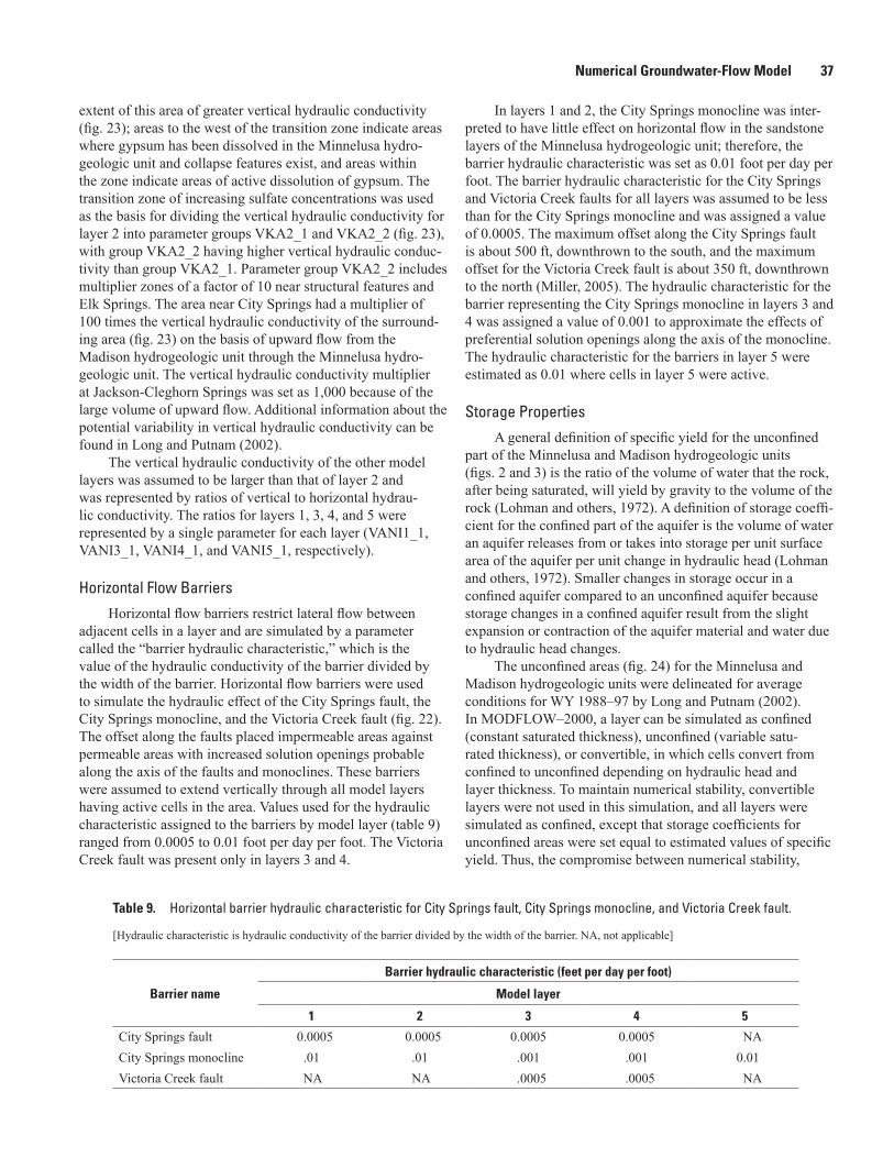
Table 9. Horizontal barrier hydraulic characteristic for City Springs fault, City Springs monocline, and Victoria Creek fault.
[Hydraulic characteristic is hydraulic conductivity of the barrier divided by the width of the barrier. NA, not applicable]
Barrier name
Barrier hydraulic characteristic (feet per day per foot)
Model layer
1 2 3 4 5
City Springs fault 0.0005 0.0005 0.0005 0.0005 NACity Springs monocline .01 .01 .001 .001 0.01Victoria Creek fault NA NA .0005 .0005 NA
Numerical Groundwater-Flow Model 37
extent of this area of greater vertical hydraulic conductivity (fig. 23); areas to the west of the transition zone indicate areas where gypsum has been dissolved in the Minnelusa hydro-geologic unit and collapse features exist, and areas within the zone indicate areas of active dissolution of gypsum. The transition zone of increasing sulfate concentrations was used as the basis for dividing the vertical hydraulic conductivity for layer 2 into parameter groups VKA2_1 and VKA2_2 (fig. 23), with group VKA2_2 having higher vertical hydraulic conduc-tivity than group VKA2_1. Parameter group VKA2_2 includes multiplier zones of a factor of 10 near structural features and Elk Springs. The area near City Springs had a multiplier of 100 times the vertical hydraulic conductivity of the surround-ing area (fig. 23) on the basis of upward flow from the Madison hydrogeologic unit through the Minnelusa hydro-geologic unit. The vertical hydraulic conductivity multiplier at Jackson-Cleghorn Springs was set as 1,000 because of the large volume of upward flow. Additional information about the potential variability in vertical hydraulic conductivity can be found in Long and Putnam (2002).
The vertical hydraulic conductivity of the other model layers was assumed to be larger than that of layer 2 and was represented by ratios of vertical to horizontal hydrau-lic conductivity. The ratios for layers 1, 3, 4, and 5 were represented by a single parameter for each layer (VANI1_1, VANI3_1, VANI4_1, and VANI5_1, respectively).
Horizontal Flow BarriersHorizontal flow barriers restrict lateral flow between
adjacent cells in a layer and are simulated by a parameter called the “barrier hydraulic characteristic,” which is the value of the hydraulic conductivity of the barrier divided by the width of the barrier. Horizontal flow barriers were used to simulate the hydraulic effect of the City Springs fault, the City Springs monocline, and the Victoria Creek fault (fig. 22). The offset along the faults placed impermeable areas against permeable areas with increased solution openings probable along the axis of the faults and monoclines. These barriers were assumed to extend vertically through all model layers having active cells in the area. Values used for the hydraulic characteristic assigned to the barriers by model layer (table 9) ranged from 0.0005 to 0.01 foot per day per foot. The Victoria Creek fault was present only in layers 3 and 4.
In layers 1 and 2, the City Springs monocline was inter-preted to have little effect on horizontal flow in the sandstone layers of the Minnelusa hydrogeologic unit; therefore, the barrier hydraulic characteristic was set as 0.01 foot per day per foot. The barrier hydraulic characteristic for the City Springs and Victoria Creek faults for all layers was assumed to be less than for the City Springs monocline and was assigned a value of 0.0005. The maximum offset along the City Springs fault is about 500 ft, downthrown to the south, and the maximum offset for the Victoria Creek fault is about 350 ft, downthrown to the north (Miller, 2005). The hydraulic characteristic for the barrier representing the City Springs monocline in layers 3 and 4 was assigned a value of 0.001 to approximate the effects of preferential solution openings along the axis of the monocline. The hydraulic characteristic for the barriers in layer 5 were estimated as 0.01 where cells in layer 5 were active.
Storage PropertiesA general definition of specific yield for the unconfined
part of the Minnelusa and Madison hydrogeologic units (figs. 2 and 3) is the ratio of the volume of water that the rock, after being satu rated, will yield by gravity to the volume of the rock (Lohman and others, 1972). A definition of storage coeffi-cient for the confined part of the aquifer is the volume of water an aquifer releases from or takes into storage per unit surface area of the aquifer per unit change in hydraulic head (Lohman and others, 1972). Smaller changes in storage occur in a confined aquifer compared to an unconfined aquifer because storage changes in a confined aquifer result from the slight expansion or contraction of the aquifer mate rial and water due to hydraulic head changes.
The unconfined areas (fig. 24) for the Minnelusa and Madison hydrogeologic units were delineated for average conditions for WY 1988–97 by Long and Putnam (2002). In MODFLOW–2000, a layer can be simulated as confined (constant saturated thickness), unconfined (variable satu-rated thickness), or convertible, in which cells convert from confined to unconfined depending on hydraulic head and layer thickness. To maintain numerical stability, convertible layers were not used in this simulation, and all layers were simulated as confined, except that storage coefficients for unconfined areas were set equal to estimated values of specific yield. Thus, the compromise between numerical stability,

Figure 24. Model cells with storage represented by unconfined storage coefficient.
MEADE CO
LAW
REN
CE
CO
PENNINGTON CO
MEA
DE
CO
PENNINGTON CO
CUSTER CO
Nemo
Caputa
Hayward
Tilford
Piedmont
Box Elder
Blackhawk
Rockerville
Farmingdale
R. 8 E.
Elk
Boxelder
Rapid
Spring
Rapid City
Gulch
Creek
T. 5 N.
T. 3 N.
T. 4 N.
T. 1 S.
T. 2 N.
T. 1 N.
T. 2 S.
R. 6 E. R. 7 E.
R. 9 E.
R. 10 E.
103°07’30”
103°22’30”
43°55’
44°15’
44°05’
16
I-90
I-90
Creek
Creek
Creek
Creek
EXPLANATION
Base from U.S. Geological Survey digital data, 1977, 1:100,000, and Rapid City, Office of City Engineer map, 2005, 1:18,000 Universal Transverse Mercator projection, Zone 13
Victoria Creek
Deadm
an
Battle Creek
Little Elk
RockervilleGulch
79
Hisega
0 4 62 8 MILES
0 642 8 KILOMETERS
44
4479
Model cells represented with unconfined storage coefficientLayer 1 (storage coefficient = 0.09)
Layer 2 (storage coefficient = 0.03)
Layer 3 (storage coefficient = 0.09)
Layer 4 (storage coefficient = 0.03)
White area to the east is continuation of layers 1–4, with a confined storage coefficient of 0.0003.
38 Numerical Groundwater-Flow Model of the Minnelusa and Madison Hydrogeologic Units, Rapid City Area, S. Dak.

Numerical Groundwater-Flow Model 39
particularly for inverse modeling, and physical accuracy was to assume that hydraulic conductivity did not change with hydraulic head in unconfined areas. Also, the actual uncon-fined areas move up and down dip as water levels fluctuate, but their general shape and total areal coverage change negli-gibly. Therefore, unconfined areas were simulated as spatially fixed. Unconfined areas for layers 1–4 were represented in the simulation by assigning storage coefficient values that were much higher than for the confined areas to the east. As esti-mated by Long and Putnam (2002), the storage coefficient in unconfined areas (specific yield) was 0.09 for the upper parts of the hydrogeologic units (layers 1 and 3) and 0.03 for the lower parts of the hydrogeologic units (layers 2 and 4). The storage coefficient for all confined areas was 0.0003.
Specific storage, which is the storage coefficient divided by the aquifer thickness, is the required storage property in MODFLOW–2000. Therefore, the storage coefficients were divided by arrays of thickness for each model layer to create the required specific storage input.
Steady-State Calibration
The steady-state model was calibrated by using a hypothetical simulation of estimated average conditions with no changes in storage. A sensitivity analysis showed model parameters that were most sensitive to steady-state observa-tions, and these parameters were optimized with inverse modeling as described in the following section. Comparisons of simulated steady-state hydraulic head values and flows to observed values and estimated flows were used to calibrate the model. The observed hydraulic head values used for steady-state calibration were based on 10-year average hydraulic head values for WY1988–97 for 176 wells completed in the Minnelusa hydrogeologic unit and 76 wells completed in the Madison hydrogeologic unit (Long and Putnam, 2002); selected information for these wells is presented in tables 20 and 21 in the “Supplemental Information” section. Forty interpolated hydraulic head values, 20 for model layer 1 and 20 for model layer 3 (table 22 in “Supplemental Informa-tion” section), were added to constrain the model in locations where information was sparse. These hydraulic head values were interpolated from the estimated average potentiometric contours for WY 1988–97 for the Minnelusa and Madison aquifers (Long and Putnam, 2002). The observed (measured) hydraulic head values (figs. 25 and 26) predominantly were available near the outcrops of the Minnelusa and Madison hydrogeologic units, whereas the interpolated hydraulic heads were used in areas east of the outcrops where measured water-level data were sparse. Estimated springflow and regional outflow (Anderson and others, 1999; Long and Putnam, 2002) also were used for steady-state flow calibration.
Standard deviation of measurement error (SDME) was used in the MODFLOW–2000 observation process for weight-ing observations and estimates for inverse modeling, in which the weight assigned to an observation or estimate was the inverse of the implied accuracy. The implied accuracy was 1 ft for observation wells with surveyed altitudes and continuous water-level records, 5 ft for wells with multiple measurements, and 10 ft for wells with water levels estimated from well driller’s completion reports or potentiometric surfaces. The implied accuracy was 0.1 ft3/s for discharge from Jackson-Cleghorn Springs, City Springs, and Deadwood Avenue Springs, and 0.2 ft3/s for discharge from other springs. Implied accuracy for discharge at the eastern boundary was 0.1 ft3/s.
Sensitivity AnalysisComposite-scaled sensitivity is the square root of the
sum of squared scaled sensitivity values for all observations divided by the number of observations. Composite-scaled sensitivity indicates the information content of all of the observations for the estimation of the parameter (Hill and others, 2000). The composite-scaled sensitivities for hydrau-lic properties represented as parameters (table 10) indicated the parameters most sensitive to steady-state observations. Parameters with composite-scaled sensitivities greater than 1.2 were selected for optimization with inverse modeling. If some parameters have composite-scaled sensitivities that are less than about 0.01 times the largest composite-scaled sensitivity, the regression has trouble converging (Hill, 1998). Optimi-zation for parameters that had composite-scaled sensitivity values less than 1.2 did not converge with reasonable values for the less-sensitive parameters.
The sensitivity of a parameter is related to the amount of information that is available to constrain the parameter. The ratio of the smallest to the largest composite-scaled sensitivities for the 12 parameters selected for optimization with parameter estimation (fig. 27) was 0.06 (ratio of sensi-tivities of DWSPR to HK3_2). The model was sensitive to most horizontal hydraulic conductivity parameters except parameter HK3_3, which represented the area in model layer 3 where the hydraulic gradient was very steep. Sensi-tivity to vertical hydraulic conductivity parameters was low except for VKA2_2 (fig. 23 and table 10), which represents an area in model layer 2 that extends east about 2 to 4 mi from the outcrop of the Minnelusa hydrogeologic unit. The model was substantially more sensitive to conductance for the cells in layer 3 that represented Jackson-Cleghorn Springs (CLEGmdsn) than conductance for other springs. The model was relatively insensitive to conductance parameters for head-dependent cells representing the eastern boundary (MnlsEB and MdsnEB; table 10).
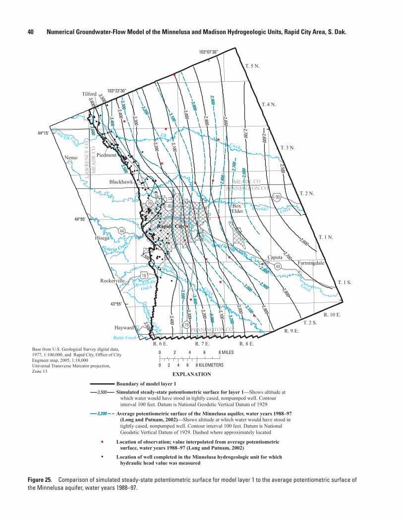
Figure 25. Comparison of simulated steady-state potentiometric surface for model layer 1 to the average potentiometric surface of the Minnelusa aquifer, water years 1988–97.
MEADE CO
LAW
REN
CE
CO
PENNINGTON CO
MEA
DE
CO
PENNINGTON CO
CUSTER CO
Nemo
Caputa
Hayward
Tilford
Piedmont
Box Elder
Blackhawk
Farmingdale
R. 8 E.
Elk
Boxelder
Rapid
Spring
Creek
Rapid City
Gulch
Creek
T. 5 N.
T. 3 N.
T. 4 N.
T. 1 S.
T. 2 N.
T. 1 N.
T. 2 S.
R. 6 E. R. 7 E.
R. 9 E.
R. 10 E.
103°07’30”
103°22’30”
43°55’
44°15’
44°05’
16
I-90
I-90
Creek
Creek
Creek
EXPLANATION
Base from U.S. Geological Survey digital data, 1977, 1:100,000, and Rapid City, Office of City Engineer map, 2005, 1:18,000 Universal Transverse Mercator projection, Zone 13
Victoria Creek
Deadm
an
Battle Creek
Little Elk
RockervilleGulch
79
Hisega
Rockerville
Victoria Creek
44
44
79
2,900
2,800
3,000
3,100
3,200
3,300
2,700 2,600
3,400
3,500
2,500
3,600
3,4003,5003,500
2,900
3,000
3,200
3,300
3,100
2,8002,700
2,600
3,400
3,200 3,100
3,3002,900
2,800
3,400
2,70
03,500
2,60
0
3,500
3,000
3,300
3,600
2,9003,000
3,100
3,200
2,80
0
Simulated steady-state potentiometric surface for layer 1—Shows altitude at which water would have stood in tightly cased, nonpumped well. Contour interval 100 feet. Datum is National Geodetic Vertical Datum of 1929
Average potentiometric surface of the Minnelusa aquifer, water years 1988–97 (Long and Putnam, 2002)—Shows altitude at which water would have stood in tightly cased, nonpumped well. Contour interval 100 feet. Datum is National Geodetic Vertical Datum of 1929. Dashed where approximately located
Location of observation; value interpolated from average potentiometric surface, water years 1988–97 (Long and Putnam, 2002)
Location of well completed in the Minnelusa hydrogeologic unit for which hydraulic head value was measured
Boundary of model layer 13,500
0 4 62 8 MILES
0 642 8 KILOMETERS
3,200
40 Numerical Groundwater-Flow Model of the Minnelusa and Madison Hydrogeologic Units, Rapid City Area, S. Dak.
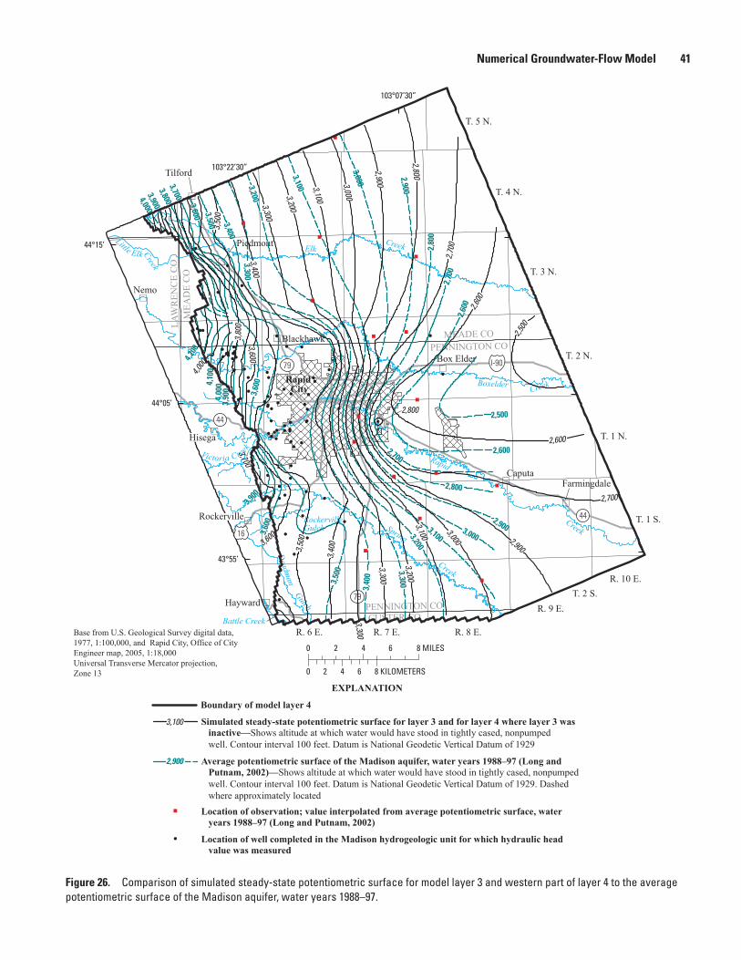
Figure 26. Comparison of simulated steady-state potentiometric surface for model layer 3 and western part of layer 4 to the average potentiometric surface of the Madison aquifer, water years 1988–97.
MEADE CO
LAW
REN
CE
CO
PENNINGTON CO
MEA
DE
CO
PENNINGTON CO
CUSTER CO
Nemo
Caputa
Hisega
Hayward
Box Elder
Blackhawk
Rockerville
R. 8 E.
Elk
Boxelder
Rapid
Spring
Rapid City
Gulch
Creek
T. 5 N.
T. 3 N.
T. 4 N.
T. 1 S.
T. 2 N.
T. 1 N.
T. 2 S.
R. 6 E. R. 7 E.
R. 9 E.
R. 10 E.
103°07’30”
103°22’30”
43°55’
44°15’
44°05’
16
I-90
Creek
Creek
Creek
Creek
Base from U.S. Geological Survey digital data, 1977, 1:100,000, and Rapid City, Office of City Engineer map, 2005, 1:18,000 Universal Transverse Mercator projection, Zone 13
Victoria Creek
Deadm
an
Battle Creek
Little Elk
RockervilleGulch
79
79
Tilford
Piedmont
Farmingdale
0 4 62 8 MILES
0 642 8 KILOMETERS
44
442,5
00
2,600
2,70
0
2,800
2,9003,000
3,1003,2003,300
3,400
3,50
0
3,600
3,80
0
4,000
2,600
2,700
2,900
3,000
3,100
3,200
3,300
3,300
3,40
0
3,50
0
3,600
3,700
2,800
3,100
3,200
3,60
0
3,000
2,900
2,800
3,700
2,600
3,800
3,900
2,500
4,10
0
4,200
4,000
4,00
03,
900
3,900
3,500
3,600
3,400
3,3003,200
3,000
3,60
0
2,80
0
2,70
02,
600
2,700
2,9003,100
3,300
3,40
0
3,50
0
Simulated steady-state potentiometric surface for layer 3 and for layer 4 where layer 3 was inactive—Shows altitude at which water would have stood in tightly cased, nonpumped well. Contour interval 100 feet. Datum is National Geodetic Vertical Datum of 1929
Average potentiometric surface of the Madison aquifer, water years 1988–97 (Long and Putnam, 2002)—Shows altitude at which water would have stood in tightly cased, nonpumped well. Contour interval 100 feet. Datum is National Geodetic Vertical Datum of 1929. Dashed where approximately locatedLocation of observation; value interpolated from average potentiometric surface, water years 1988–97 (Long and Putnam, 2002)
Location of well completed in the Madison hydrogeologic unit for which hydraulic head value was measured
3,100
Boundary of model layer 4
EXPLANATION
2,900
Numerical Groundwater-Flow Model 41

Table 10. Composite-scaled sensitivities for hydraulic properties represented as parameters.
[Shading indicates that parameter values were estimated by inverse modeling. Composite-scaled sensitivity calculated for final parameter values]
Parameter name Location map Parameter descriptionComposite-scaled
sensitivity
CLEGmdsn Jackson-Cleghorn Springs, fig. 12 Conductance parameter is the hydraulic conduc tivity of the interface between the head-dependent cells times the cell area divided by the thickness
4.63CLEGmnls Jackson-Cleghorn Springs, fig. 12 .39CITYSPR City Springs, fig. 12 .19DWSPR Deadwood Avenue Springs, fig. 12 1.25BESPR Boxelder Springs, fig. 12 .15ELKSPR Elk Springs, fig. 11 .05GAL Infiltration Gallery Springs, fig. 12 .03CLAKE Canyon Lake, fig. 12 .16HK1_1 Fig. 17 Horizontal hydraulic conductivity parameters for model
layer 12.38
HK1_2 Fig. 17 16.96HK1_3 Fig. 17 5.98HK3_1 Fig. 19 Horizontal hydraulic conductivity parameters for model
layer 31.29
HK3_2 Fig. 19 21.42HK3_3 Fig. 19 1.13HK3_4 Fig. 19 15.51HK3_5 Fig. 19 8.63HK3_6 Fig. 19 2.24HK3_7 Fig. 19 5.70HANI3_2 Fig. 19 Anisotropy for area represented by parameter group HK3_1 .03HK5_1 Fig. 22 Horizontal hydraulic conductivity for layer 5 .83VANI1_1 Active cells in model layer 1, fig. 8 Ratio of vertical to horizontal hydraulic conductivity for
model layer 1.01
VKA2_1 Fig. 23 Vertical hydraulic conductivity for model layer 2 .20VKA2_2 Fig. 23 4.13VANI3_1 Active cells in model layer 3, fig. 9 Ratio of vertical to horizontal hydraulic conductivity for
model layer 3.01
VANI4_1 Active cells in model layer 4, fig. 9 Ratio of vertical to horizontal hydraulic conductivity for model layer 4
.04
VANI5_1 Fig. 22 Ratio of vertical to horizontal hydraulic conductivity for model layer 5
.01
MnlsEB Fig. 8 Conductance parameter is the hydraulic conduc tivity of the interface between the head-dependent cell at the eastern boundary times the area divided by the thickness
.01MdsnEB Fig. 9 .01
42 Numerical Groundwater-Flow Model of the Minnelusa and Madison Hydrogeologic Units, Rapid City Area, S. Dak.

Figure 27. Composite-scaled sensitivities for parameter values that were determined with inverse modeling in steady-state simulation.
0
5
10
15
20
25
HK1_
1
HK1_
2
HK1_
3
HK3_
1
HK3_
2
HK3_
4
HK3_
5
HK3_
6
HK3_
7
VKA2
_2
CLEG
mds
n
DWSP
R
COM
POSI
TE-S
CALE
D SE
NSI
TIVI
TY
PARAMETER (SEE TABLE 10 FOR DESCRIPTION)
Numerical Groundwater-Flow Model 43
Comparison of Simulated and Observed Steady-State Hydraulic Head Values
Linear regression between the 252 simulated and observed hydraulic head values for the steady-state simula-tion had a coefficient of determination (R2 value) of 0.92 with an average arithmetic dif ference of -7.6 ft and an average absolute difference of 37.6 ft. Most of the observed hydraulic heads used for comparison with simulated hydraulic heads were between 3,400 and 3,600 ft above NGVD 29 (fig. 28). A histogram of residuals between the 252 simulated and observed hydraulic head values (fig. 29) shows that about 65 percent of the residuals were less than ±40 ft.
The simulated potentiometric surface for model layer 1 overlain on the average potentiometric surface for WY 1988–97 generally shows similar gradients in hydrau-lic head values, with the largest differences near the model boundaries (fig. 25). The differences between simulated and observed (average for WY 1988–97) hydraulic head values for the Minnelusa hydrogeologic unit in the detailed study area were within ±30 ft for 73.7 percent of the observation wells (fig. 30). The difference between observed and simulated hydraulic head values that were not within ±30 ft for some of the wells could be related to the effect of unknown breccia pipes or karst features that were not represented in the model.
The simulated potentiometric surface for model layer 3 matched the observed steep hydraulic gradients in eastern Rapid City (fig. 26). The differences between simulated and observed hydraulic head values for the Madison hydrogeo-logic unit in the detailed study area were within ±30 ft for 76.9 percent of the observation wells (fig. 31). Wells with a
hydraulic head difference that was not within ±30 ft generally were near the western model boundary.
Comparison of Simulated and Estimated Steady-State Flow
Total simulated steady-state springflow of 31.6 ft3/s was similar to the sum of estimated springflow of 32.8 ft3/s (table 11). Simulated discharge from Jackson-Cleghorn Springs was 20.5 ft3/s compared to the estimated value of 21.6 ft3/s. Simulated regional outflow from model layers 1 and 2 at the eastern boundary of 12.9 ft3/s was slightly larger than the estimated value of 12.3 ft3/s from Long and Putnam (2002). Simulated regional outflow from model layers 3 and 4 of 12.8 ft3/s was slightly larger than the estimated value of 12.2 ft3/s from Long and Putnam (2002).
Transient Calibration
The transient calibration was accomplished by simulat-ing transient conditions for WY 1988–97 divided into twenty 6-month stress periods. Comparisons of simulated transient hydraulic head values and flows to observed values and estimated flows were used to calibrate the model. Simulated transient hydraulic head values were compared to observed (measured) hydraulic head values for 19 observation wells completed in the Minnelusa and Madison hydrogeologic units (fig. 32); water-level records were available for these 19 obser-vation wells for all or parts of the transient simulation. Tran-sient springflow was calibrated to springflow measurements

Figure 29. Histograms of residuals between simulated steady-state and observed (average for water years 1988–97) hydraulic head values.
Figure 28. Residuals between simulated steady-state and observed hydraulic head values and their relation to average (water years 1988–97) hydraulic head values.
0
50
100
150
200
2,500 3,000 3,500 4,000 4,500
HYDR
AULI
C HE
AD R
ESID
IUAL
, IN
FEE
T
AVERAGE HYDRAULIC HEAD, WATER YEARS 1988−97 IN FEET ABOVE NATIONAL GEODETIC VERTICAL DATUM OF 1929
Minnelusa hydrogeologic unit
Madison hydrogeologic unit
-200
-150
-100
-50
0
5
10
15
20
25
0 40 80 120 160 200
FREQ
UEN
CY, I
N P
ERCE
NT
HYDRAULIC HEAD RESIDUAL, IN FEET
-200 -160 -120 -80 -40
44 Numerical Groundwater-Flow Model of the Minnelusa and Madison Hydrogeologic Units, Rapid City Area, S. Dak.

Figure 30. Differences between simulated steady-state and observed (average for water years 1988–97) hydraulic head values for the Minnelusa hydrogeologic unit in the detailed study area.
44°05’
I-90
44
79
Rapid
16
Creek
Boxelder
Spring Creek
CreekMEADE CO
PENNINGTON CO
T. 1 N.
T. 1 S.
R. 7 E.
R. 6 E.
R. 5 E.
103°22’30”
103°15’
44°00’
T. 3 N.
T. 2 N.
Base fom U.S. Geological Survey digital data, 1977, 1:100,000 Rapid City, Office of City Engineer map, 2005, 1:18,000Unversal Transverse Mercator projectionZone 13
0 2 31 4 MILES
0 1 2 3 4 KILOMETERS
79
44
16
Rapid
Creek
Boundary of model layer 1
3,350
3,300
3,150
3,400
3,45
03,5
00
3,0003,400
3,450
3,200 3,100
3,300
3,250
3,200
3,100
3,050
3,150
3,2503,350
3,400
1.0 4.1 8.1
34.339.4 9.1 3.0 1.0
90 to less than 12060 to less than 9030 to less than 600 to less than 30Less than 0 to greater than -30-30 to greater than -60-60 to greater than -90-90 to greater than -120
Frequency ofdifferencecategory Difference, in feet
Simulated steady-state potentiometric surface for model layer 1—Shows altitude at which water would have stood in tightly cased, nonpumped well. Contour interval 50 feet. Datum is National Geodetic Vertical Datum of 1929
3,500
EXPLANATION
Rapid CityRapid City
Numerical Groundwater-Flow Model 45

Figure 31. Differences between simulated steady-state and observed (average for water years, 1988–97) hydraulic head values for the Madison hydrogeologic unit in the detailed study area.
44°05’
I-90
44
79
Rapid
16
Creek
Boxelder
Spring Creek
Creek MEADE COPENNINGTON CO
T. 1 N.
T. 1 S.
R. 7 E.
R. 6 E.
R. 5 E.
103°22’30”
103°15’
44°00’
T. 3 N.
T. 2 N.
Base fom U.S. Geological Survey digital data, 1977, 1:100,000 Rapid City, Office of City Engineer map, 2005, 1:18,000Unversal Transverse Mercator projectionZone 13
0 2 31 4 MILES
0 1 2 3 4 KILOMETERS
79
44
16
Rapid
CreekRapid CityRapid City
3,425
3,47
5
3,47
5
3,425
3,450
3,45
0
3,425
3,100
3,2003,300
3,400
3,000
2,90
02,
800
2,700
3,50
0
3,60
0
3,70
0
3,60
0
3,50
0
3,500
3,600
3,2003,100
3,0002,900
2,800
2,700
3,4003,400
3,300
3,400
2,600
Supplemental contours 3,425, 3,450, and 3,4753,475
Difference, in feet 1.9 .0 7.7
30.846.1 5.8 5.8 1.9
90 to less than 12060 to less than 9030 to less than 600 to less than 30Less than 0 to greater than -30-30 to greater than -60-60 to greater than -90-90 to greater than -120
Simulated steady-state potentiometric surface for model layer 3—Shows altitude at which water would have stood in tightly cased, nonpumped well. Contour interval 100 feet. Datum is National Geodetic Vertical Datum of 1929
3,600
EXPLANATIONBoundary of model layer 3
Frequency ofdifferencecategory
46 Numerical Groundwater-Flow Model of the Minnelusa and Madison Hydrogeologic Units, Rapid City Area, S. Dak.

Table 11. Steady-state springflow estimates and simulated springflow.
[Springflow rates in cubic feet per second]
Spring nameSteady-state springflow
(from table 6) Simulated springflow
Arithmetic difference
Jackson-Cleghorn Springs 121.6 20.5 -1.1City Springs 21.7 1.4 -.3Deadwood Avenue Springs 22.8 2.6 -.2Boxelder Springs 21.0 1.8 .8Elk Springs 23.7 4.2 .5Infiltration Gallery Springs 11.5 .5 -1.0Canyon Lake 3.5 .6 .1Total 32.8 31.6 -1.2
1Anderson and others, 1999.2Long and Putnam, 2002.3No quantitative measurements were available; small discharge was assumed because of hydraulic connection.
Numerical Groundwater-Flow Model 47
or estimated springflow for seven springs (figs. 11 and 12). The estimated springflow for some of the springs represented an average discharge. Regional outflow at the eastern model boundary was calibrated to estimated average regional outflow used in the steady-state simulation. The regional outflow was assumed to be relatively constant because the boundary was about 20 mi east of most recharge, spring discharge, and pumping areas.
Comparison of Simulated and Observed Transient Hydraulic Head Values
The average absolute difference between simulated and observed hydraulic head values for the 19 observation wells ranged from 3.5 to 65.1 ft with a median value of 18.3 ft (table 12). Hydrographs of simulated and observed hydraulic head values for 18 of the wells (fig. 33) show the response of the heads to stresses. Hydrographs for the nested wells completed in both the Minnelusa and Madison hydrogeo-logic units at six sites are presented adjacent to each other. In general, the magnitude of changes in simulated hydraulic head values were less than the observed changes.
The changes in simulated hydraulic head values for wells 104 and 1 between stress periods are much less than observed changes. The simulated hydraulic head for well 104 does not increase as quickly as the observed hydraulic head during the wet period (late 1990s; stress periods 12–20). Wells 104 and 1 are located at the northern no-flow boundary (figs. 32, 8, and 9), which may have damped hydraulic head response. Simulated hydraulic head values for wells 124 and 3 were similar in trend; however, the simulated hydraulic head
values for well 3 were about 50 ft higher than observed values. Simulated hydraulic head values for wells 200 and 33 were similar to observed hydraulic head values; however, declines during the dry period and increases during the wet period were less for the simulated values.
Simulated hydraulic head values for wells 223 and 46 were similar to observed hydraulic head values; however, the influence of pumping resulted in some fluctuations in observed hydraulic head that were not matched in the simulated values, probably because of smoothing from using 6-month stress periods. Simulated hydraulic head values for wells 229 and 50 were similar to observed hydraulic head values. Simulated hydraulic head values for well 272 were similar in trend but consistently about 50 ft below observed values. Simulated and observed hydraulic head values for well 68 were very similar.
Simulated hydraulic head values for well 181 were similar in trend and consistently about 20 ft above observed values. Simulated hydraulic head values for well 209 were similar to observed hydraulic head values; however, simulated hydraulic head values were smoothed compared to observed values. Simulated hydraulic head values for wells 224 and 233 were similar to observed values. The simulated hydrau-lic head values for well 15 (table 12) were about 60 ft below observed values. Well 15 had only four observations (not shown in fig. 33) and is located near the western model bound-ary. Simulated hydraulic head values for well 47 were about 35 ft above observed values and were steady in comparison to observed values. Simulated hydraulic head values for well 43 were influenced by pumping in a nearby well, resulting in large fluctuation in observed hydraulic head values; however, the simulated values were similar to the recovered hydraulic head values.

Figure 32. Locations of observation wells with transient hydraulic head values.
MEADE CO
LAW
REN
CE
CO
PENNINGTON CO
MEA
DE
CO
PENNINGTON CO
CUSTER CO
Nemo
Caputa
Hayward
Tilford
Piedmont
Box Elder
Blackhawk
Farmingdale
R. 8 E.
Elk
Boxelder
Rapid
Spring
Rapid City
Gulch
Creek
T. 5 N.
T. 3 N.
T. 4 N.
T. 1 S.
T. 2 N.
T. 1 N.
T. 2 S.
R. 6 E. R. 7 E.
R. 9 E.
R. 10 E.
103°07’30”
103°22’30”
43°55’
44°15’
44°05’
16
I-90
I-90
Creek
Creek
Creek
Base from U.S. Geological Survey digital data, 1977, 1:100,000, and Rapid City, Office of City Engineer map, 2005, 1:18,000 Universal Transverse Mercator projection, Zone 13
Victoria Creek
Deadm
an
Battle Creek
Little Elk
RockervilleGulch
79
Creek
Hisega
Rockerville
Victoria Creek
0 4 62 8 MILES
0 642 8 KILOMETERS
44
4479
209
229, 50233
224
200, 33
47
181
272, 68
124, 3
15
223, 46
104, 1
43
272, 68
272, 68
EXPLANATION
Outcrop of Minnelusa hydrogeologic unit
Outcrop of Madison hydrogeologic unit
Observation well completed in Minnelusa hydrogeologic unit and number (table 20)
Observation well completed in Madison hydrogeologic unit and number (table 21)
Note: comma-separated site numbers indicate nested wells in Minnelusa (first number) and Madison (second number) hydrogeologic units
Geologic outcrops modified from Strobel and others, 1999
48 Numerical Groundwater-Flow Model of the Minnelusa and Madison Hydrogeologic Units, Rapid City Area, S. Dak.
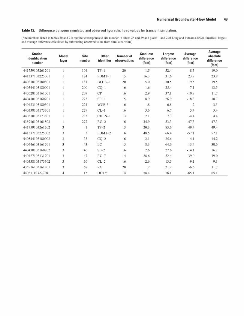
Table 12. Difference between simulated and observed hydraulic head values for transient simulation.
[Site numbers listed in tables 20 and 21; number corresponds to site number in tables 28 and 29 and plates 1 and 2 of Long and Putnam (2002). Smallest, largest, and average difference calculated by subtracting observed value from simulated value]
Station identification
number
Model layer
Site number
Other identifier
Number of observations
Smallest difference
(feet)
Largest difference
(feet)
Average difference
(feet)
Average absolute
difference (feet)
441759103261201 1 104 TF–1 20 1.5 52.4 -8.3 19.0441337103225001 1 124 PDMT–1 15 16.3 31.6 23.8 23.8440818103180801 1 181 BLHK–1 20 5.0 30.5 19.5 19.5440544103180001 1 200 CQ–1 16 1.6 25.4 -7.1 13.5440528103161001 1 209 CP 16 2.9 37.1 -10.8 11.7440430103160201 1 223 SP–1 15 8.9 26.9 -18.3 18.3440423103180501 1 224 WCR-3 16 .8 6.8 .2 3.5440338103173301 1 229 CL–1 16 3.6 6.7 5.4 5.4440310103173801 1 233 CHLN–1 13 2.1 7.3 -4.4 4.4435916103161802 1 272 RG–2 6 34.9 53.3 -47.3 47.3441759103261202 3 1 TF–2 13 20.3 83.6 49.4 49.4441337103225002 3 3 PDMT–2 6 48.5 66.4 -57.1 57.1440544103180002 3 33 CQ–2 16 2.1 25.6 -4.1 14.2440446103161701 3 43 LC 15 8.3 64.6 13.4 30.6440430103160202 3 46 SP–2 16 2.6 27.6 -14.1 16.2440427103131701 3 47 RC–7 14 28.6 52.4 39.0 39.0440338103173302 3 50 CL–2 16 2.6 13.5 -9.1 9.1435916103161801 3 68 RG 20 .2 21.2 -6.6 11.7440811103222201 4 15 DOTY 4 58.4 76.1 -65.1 65.1
Numerical Groundwater-Flow Model 49

Figure 33. Simulated and observed hydraulic head values for model layers 1 and 3.
3,560
3,580
3,600
3,620
3,640
3,660
3,680
3,700
Site 1 (TF−2) MADISON
3,560
3,580
3,600
3,620
3,640
3,660
3,680
3,700
HYDR
AULI
C HE
AD, I
N F
EET
ABOV
E N
ATIO
NAL
GEO
DETI
C VE
RTIC
AL D
ATUM
OF
1929
Site 104 (TF−1) MINNELUSA
3,440
3,460
3,480
3,500
3,520
3,540
3,560
3,580
Site 124 (PDMT−1) MINNELUSA
3,500
3,520
3,540
3,560
3,580
3,600
3,620
3,640
Site 3 (PDMT−2) MADISON
3,400
3,420
3,440
3,460
3,480
3,500
3,520
3,540
WATER YEAR
Site 200 (CQ−1) MINNELUSA
3,400
3,420
3,440
3,460
3,480
3,500
3,520
3,540
Site 33 (CQ−2) MADISON
Simulated
EXPLANATION
Observed
1987 1989 1991 1993 1995 1997
WATER YEAR
1987 1989 1991 1993 1995 1997
50 Numerical Groundwater-Flow Model of the Minnelusa and Madison Hydrogeologic Units, Rapid City Area, S. Dak.
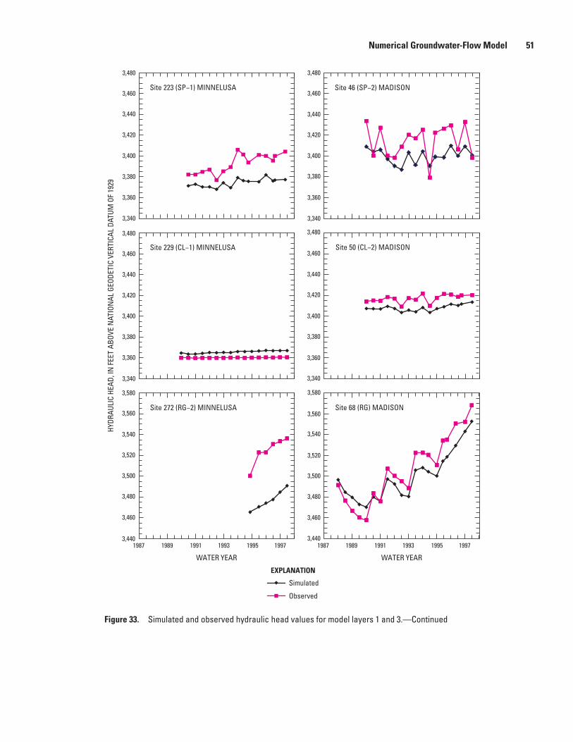
Figure 33. Simulated and observed hydraulic head values for model layers 1 and 3.—Continued
WATER YEAR
Simulated
EXPLANATION
Observed
1987 1989 1991 1993 1995 1997
WATER YEAR
1987 1989 1991 1993 1995 1997
3,340
3,360
3,380
3,400
3,420
3,440
3,460Site 46 (SP−2) MADISON
3,340
3,360
3,380
3,400
3,420
3,440
3,460Site 223 (SP−1) MINNELUSA
Site 229 (CL−1) MINNELUSA
3,340
3,360
3,380
3,400
3,420
3,440
3,460
3,480
Site 50 (CL−2) MADISON
3,440
3,460
3,480
3,500
3,520
3,540
3,560
3,580
Site 272 (RG−2) MINNELUSA
3,440
3,460
3,480
3,500
3,520
3,540
3,560
3,580
Site 68 (RG) MADISON
3,4803,480
3,340
3,360
3,380
3,400
3,420
3,440
3,460
3,480
HYDR
AULI
C HE
AD, I
N F
EET
ABOV
E N
ATIO
NAL
GEO
DETI
C VE
RTIC
AL D
ATUM
OF
1929
Numerical Groundwater-Flow Model 51

Figure 33. Simulated and observed hydraulic head values for model layers 1 and 3.—Continued
WATER YEAR
Simulated
EXPLANATION
Observed
1987 1989 1991 1993 1995 1997
WATER YEAR
1987 1989 1991 1993 1995 1997
3,340
3,360
3,380
3,400
3,420
3,440
3,460
3,480
3,380
3,400
3,420
3,440
3,460
3,480
3,500
3,520
3,340
3,360
3,380
3,400
3,420
3,440
3,460
3,480
3,340
3,360
3,380
3,400
3,420
3,440
3,460
3,480
3,100
3,120
3,140
3,160
3,180
3,200
3,220
3,240
3,320
3,340
3,360
3,380
3,400
3,420
3,440
3,460
Site 209 (CP) MINNELUSASite 181 (BLHK−1) MINNELUSA
Site 224 (WCR−3) MINNELUSA Site 233 (CHLN−1) MINNELUSA
Site 47 (RC−7) MADISON Site 43 (LC) MADISON
HYDR
AULI
C HE
AD, I
N F
EET
ABOV
E N
ATIO
NAL
GEO
DETI
C VE
RTIC
AL D
ATUM
OF
1929
52 Numerical Groundwater-Flow Model of the Minnelusa and Madison Hydrogeologic Units, Rapid City Area, S. Dak.
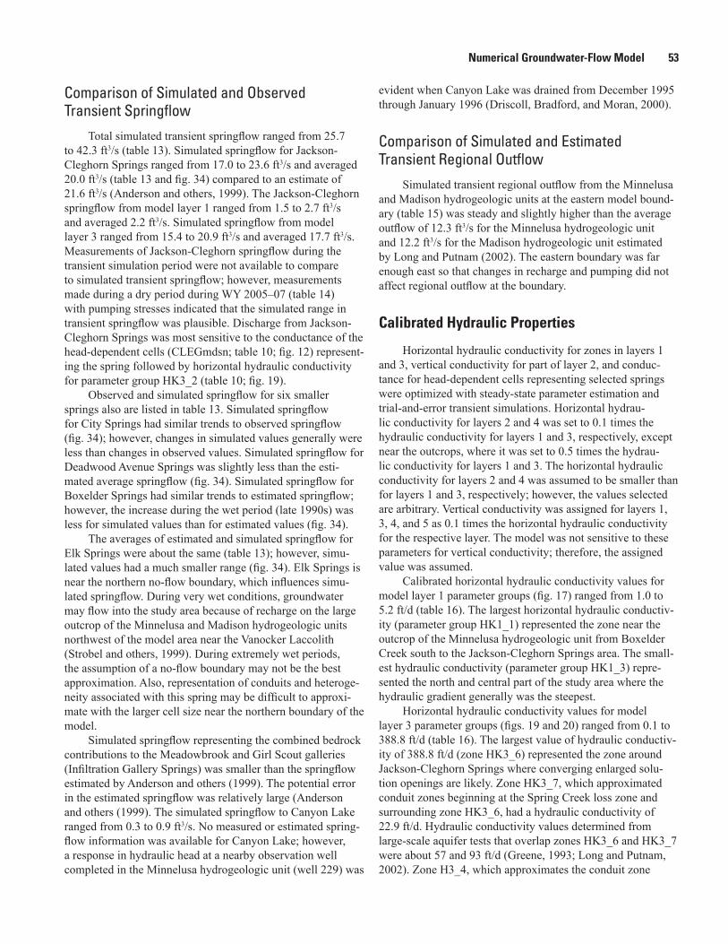
Numerical Groundwater-Flow Model 53
Comparison of Simulated and Observed Transient Springflow
Total simulated transient springflow ranged from 25.7 to 42.3 ft3/s (table 13). Simulated springflow for Jackson-Cleghorn Springs ranged from 17.0 to 23.6 ft3/s and averaged 20.0 ft3/s (table 13 and fig. 34) compared to an estimate of 21.6 ft3/s (Anderson and others, 1999). The Jackson-Cleghorn springflow from model layer 1 ranged from 1.5 to 2.7 ft3/s and averaged 2.2 ft3/s. Simulated springflow from model layer 3 ranged from 15.4 to 20.9 ft3/s and averaged 17.7 ft3/s. Measurements of Jackson-Cleghorn springflow during the transient simulation period were not available to compare to simulated transient springflow; however, measurements made during a dry period during WY 2005–07 (table 14) with pumping stresses indicated that the simulated range in transient springflow was plausible. Discharge from Jackson-Cleghorn Springs was most sensitive to the conductance of the head-dependent cells (CLEGmdsn; table 10; fig. 12) represent-ing the spring followed by horizontal hydraulic conductivity for parameter group HK3_2 (table 10; fig. 19).
Observed and simulated springflow for six smaller springs also are listed in table 13. Simulated springflow for City Springs had similar trends to observed springflow (fig. 34); however, changes in simulated values generally were less than changes in observed values. Simulated springflow for Deadwood Avenue Springs was slightly less than the esti-mated average springflow (fig. 34). Simulated springflow for Boxelder Springs had similar trends to estimated springflow; however, the increase during the wet period (late 1990s) was less for simulated values than for estimated values (fig. 34).
The averages of estimated and simulated springflow for Elk Springs were about the same (table 13); however, simu-lated values had a much smaller range (fig. 34). Elk Springs is near the northern no-flow boundary, which influences simu-lated springflow. During very wet conditions, groundwater may flow into the study area because of recharge on the large outcrop of the Minnelusa and Madison hydrogeologic units northwest of the model area near the Vanocker Laccolith (Strobel and others, 1999). During extremely wet periods, the assumption of a no-flow boundary may not be the best approximation. Also, representation of conduits and heteroge-neity associated with this spring may be difficult to approxi-mate with the larger cell size near the northern boundary of the model.
Simulated springflow representing the combined bedrock contributions to the Meadowbrook and Girl Scout galleries (Infiltration Gallery Springs) was smaller than the springflow estimated by Anderson and others (1999). The potential error in the estimated springflow was relatively large (Anderson and others (1999). The simulated springflow to Canyon Lake ranged from 0.3 to 0.9 ft3/s. No measured or estimated spring-flow information was available for Canyon Lake; however, a response in hydraulic head at a nearby observation well completed in the Minnelusa hydrogeologic unit (well 229) was
evident when Canyon Lake was drained from December 1995 through January 1996 (Driscoll, Bradford, and Moran, 2000).
Comparison of Simulated and Estimated Transient Regional Outflow
Simulated transient regional outflow from the Minnelusa and Madison hydrogeologic units at the eastern model bound-ary (table 15) was steady and slightly higher than the average outflow of 12.3 ft3/s for the Minnelusa hydrogeologic unit and 12.2 ft3/s for the Madison hydrogeologic unit estimated by Long and Putnam (2002). The eastern boundary was far enough east so that changes in recharge and pumping did not affect regional outflow at the boundary.
Calibrated Hydraulic Properties
Horizontal hydraulic conductivity for zones in layers 1 and 3, vertical conductivity for part of layer 2, and conduc-tance for head-dependent cells representing selected springs were optimized with steady-state parameter estimation and trial-and-error transient simulations. Horizontal hydrau-lic conductivity for layers 2 and 4 was set to 0.1 times the hydraulic conductivity for layers 1 and 3, respectively, except near the outcrops, where it was set to 0.5 times the hydrau-lic conductivity for layers 1 and 3. The horizontal hydraulic conductivity for layers 2 and 4 was assumed to be smaller than for layers 1 and 3, respectively; however, the values selected are arbitrary. Vertical conductivity was assigned for layers 1, 3, 4, and 5 as 0.1 times the horizontal hydraulic conductivity for the respective layer. The model was not sensitive to these parameters for vertical conductivity; therefore, the assigned value was assumed.
Calibrated horizontal hydraulic conductivity values for model layer 1 parameter groups (fig. 17) ranged from 1.0 to 5.2 ft/d (table 16). The largest horizontal hydraulic conductiv-ity (parameter group HK1_1) represented the zone near the outcrop of the Minnelusa hydrogeologic unit from Boxelder Creek south to the Jackson-Cleghorn Springs area. The small-est hydraulic conductivity (parameter group HK1_3) repre-sented the north and central part of the study area where the hydraulic gradient generally was the steepest.
Horizontal hydraulic conductivity values for model layer 3 parameter groups (figs. 19 and 20) ranged from 0.1 to 388.8 ft/d (table 16). The largest value of hydraulic conductiv-ity of 388.8 ft/d (zone HK3_6) represented the zone around Jackson-Cleghorn Springs where converging enlarged solu-tion openings are likely. Zone HK3_7, which approximated conduit zones beginning at the Spring Creek loss zone and surrounding zone HK3_6, had a hydraulic conductivity of 22.9 ft/d. Hydraulic conductivity values determined from large-scale aquifer tests that overlap zones HK3_6 and HK3_7 were about 57 and 93 ft/d (Greene, 1993; Long and Putnam, 2002). Zone H3_4, which approximates the conduit zone

Table 13. Estimated and simulated transient springflow.
[Springflow in cubic feet per second. Springflow for Jackson-Cleghorn and Infiltration Gallery Springs from Anderson and others (1999); estimate was made for water years 1988–89 and values for remaining stress periods were assumed to be similar. Springflow for City Springs from Long and Putnam (2002); flow from City Springs and some unnamed springs about 0.3 mi to the east were estimated from stream-flow record. Springflow for Deadwood Avenue, Boxelder, and Elk Springs from Long and Putnam (2002); an average value was estimated for Deadwood Avenue Springs on the basis of streamflow records for water years 1988–90. No quantitative measurements were available for Canyon Lake; small discharge was assumed]
Stress period
Jackson-Cleghorn Springs
City SpringsDeadwood Avenue
SpringsBoxelder Springs Elk Springs
Infiltration Gallery Springs
Canyon Lake Total
EstimatedSim-
ulatedEstimated
Sim-ulated
EstimatedSim-
ulatedEstimated
Sim-ulated
EstimatedSim-
ulatedEstimated
Sim-ulated
EstimatedSim-
ulatedEstimated
Sim-ulated
1 21.6 20.9 1.9 1.8 2.8 3.2 0.0 1.3 0.3 6.2 1.5 0.5 0.5 0.6 28.6 34.52 21.6 20.0 1.0 1.6 2.8 2.8 .0 1.0 .3 5.9 1.5 .5 .5 .6 27.7 32.33 21.6 19.8 1.0 1.7 2.8 3.1 .0 .9 .0 5.7 1.5 .5 .5 .7 27.4 32.44 21.6 19.7 .7 1.5 2.8 2.8 .0 .8 .0 5.4 1.5 .5 .5 .7 27.1 31.45 21.6 19.1 .8 1.5 2.8 2.9 .0 .7 .0 5.3 1.5 .5 .5 .5 27.2 30.46 21.6 19.1 .8 1.2 2.8 2.5 .0 .6 .0 5.0 1.5 .4 .5 .3 27.2 29.27 21.6 18.9 .3 1.0 2.8 2.7 .0 .6 .1 4.8 1.5 .4 .5 .4 26.8 28.88 21.6 20.8 1.3 .7 2.8 2.1 .0 1.4 .1 5.1 1.5 .4 .5 .4 27.8 31.09 21.6 19.5 .6 .9 2.8 1.9 .0 .9 .0 5.1 1.5 .4 .5 .5 27.0 29.3
10 21.6 17.0 .4 .4 2.8 1.8 .0 .6 .0 5.0 1.5 .4 .5 .5 26.8 25.711 21.6 18.4 .3 .9 2.8 2.0 .2 .5 .1 4.8 1.5 .4 .5 .5 27.0 27.512 21.6 18.1 2.1 .3 2.8 1.5 .2 2.1 .1 5.1 1.5 .4 .5 .5 28.8 28.013 21.6 20.0 1.5 .5 2.8 1.7 .0 1.3 .4 5.2 1.5 .5 .5 .7 28.3 30.0
14 21.6 17.6 1.4 .1 2.8 1.3 .0 1.9 .4 5.1 1.5 .4 .5 .6 28.2 27.115 21.6 19.3 1.3 .8 2.8 1.9 .5 1.1 8.6 5.1 1.5 .5 .5 .7 36.8 29.416 21.6 20.8 3.3 .7 2.8 2.0 .5 3.1 8.6 5.8 1.5 .5 .5 .8 38.8 33.617 21.6 21.9 2.8 1.3 2.8 2.4 2.5 1.9 8.2 6.1 1.5 .5 .5 .9 39.9 34.918 21.6 21.5 4.0 .7 2.8 1.9 2.5 3.7 8.2 6.5 1.5 .5 .5 .8 41.1 35.519 21.6 23.0 3.5 1.5 2.8 2.5 6.8 2.7 18.9 6.6 1.5 .5 .5 .8 55.6 37.620 21.6 23.6 4.9 1.5 2.8 2.8 6.8 5.9 18.9 7.2 1.5 .5 .5 .8 57.0 42.3
Average 21.6 20.0 1.7 1.0 2.8 2.3 1.0 1.7 3.7 5.6 1.5 .5 .5 .6 32.8 31.5
54
Num
erical Groundwater-Flow
Model of the M
innelusa and Madison Hydrogeologic Units, Rapid City Area, S. Dak.
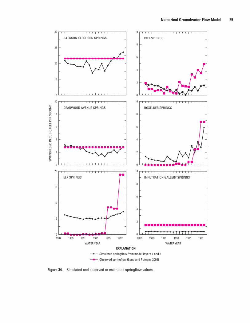
Figure 34. Simulated and observed or estimated springflow values.
EXPLANATION
1987 1989 1991 1993 1995 1997
WATER YEAR
1987 1989 1991 1993 1995 1997
WATER YEAR
0
2
4
6
8
10
10
15
20
25
30
0
2
4
6
8
10
SPRI
NGF
LOW
, IN
CUB
IC F
EET
PER
SECO
ND
0
2
4
6
8
10
0
5
10
15
20
0
2
4
6
8
10
CITY SPRINGSJACKSON-CLEGHORN SPRINGS
DEADWOOD AVENUE SPRINGS BOXELDER SPRINGS
ELK SPRINGS INFILTRATION GALLERY SPRINGS
Simulated springflow from model layers 1 and 3
Observed springflow (Long and Putnam, 2002)
Numerical Groundwater-Flow Model 55

Table 14. Jackson-Cleghorn springflow estimated from streamflow measurements on Rapid Creek.
[Upstream station is Rapid Creek at Braeburn Addition (fig. 12). Downstream station is Rapid Creek below Cleghorn Springs (fig. 12). Pumping withdrawal rate from Jackson Springs Gallery from Ron Barber, Rapid City Water Department, oral commun. (2004–05). Estimated Jackson-Cleghorn springflow calculated by subtracting streamflow at upstream station from downstream station and adding pumping withdrawal from Jackson Springs Gallery]
Date of paired streamflow
measurements
Streamflow (cubic feet per second)Pumping withdrawal rate from
Jackson Springs Gallery
(cubic feet per second)
Estimated Jackson-Cleghorn springflow
(cubic feet per second)Upstream station(440321103181101)
Downstream station (06412900)
10/19/2004 10.3 26.2 0.0 15.910/19/2004 10.7 25.2 .0 14.510/19/2004 11.0 28.6 .0 17.610/19/2004 10.2 26.5 .0 16.310/26/2004 9.9 22.8 4.0 16.910/26/2004 10.3 23.0 4.0 16.711/04/2004 10.1 24.8 4.0 18.711/04/2004 10.7 26.4 4.0 19.710/11/2005 8.3 16.6 10.0 18.310/11/2005 8.7 16.4 10.0 17.711/07/2005 6.4 19.6 4.0 17.211/07/2005 7.6 21.2 4.0 17.610/02/2006 6.3 21.2 .0 14.903/15/2007 8.5 25.2 .0 16.703/15/2007 7.9 23.5 .0 15.603/16/2007 7.2 23.2 .0 16.003/16/2007 7.0 22.0 .0 15.0
Table 15. Simulated transient regional outflow from Minnelusa and Madison hydrogeologic units at the eastern model boundary.
Stress period
Simulated regional outflow (cubic feet per second)
Minnelusa hydrogeologic unit
Madison hydrogeologic unit
1 12.9 12.92 12.9 12.63 12.9 12.94 12.8 12.85 12.9 12.96 12.8 12.87 12.9 12.98 12.8 12.79 12.8 12.8
10 12.8 12.7
Stress period
Simulated regional outflow (cubic feet per second)
Minnelusa hydrogeologic unit
Madison hydrogeologic unit
11 12.8 12.712 12.7 12.613 12.8 12.714 12.7 12.515 12.8 12.616 12.7 12.517 12.7 12.618 12.7 12.519 12.8 12.620 12.8 12.5
56 Numerical Groundwater-Flow Model of the Minnelusa and Madison Hydrogeologic Units, Rapid City Area, S. Dak.

Table 16. Calibrated horizontal hydraulic conductivity for parameters representing zones of hydraulic conductivity in model layers 1, 3, and 5.
[Location of area represented by the parameter group name is shown in figures 17, 19, 20, and 22]
Parameter group name
Model layerArea of parameter zone
(square miles)Effective horizontal hydraulic conductivity
(feet per day)
HK1_1 1 67.9 5.2HK1_2 1 566.0 3.3HK1_3 1 153.2 1.0
1HK3_1 3 46.8 16.0HK3_2 3 596.3 5.4HK3_3 3 56.8 .1HK3_4 3 28.9 39.3HK3_5 3 91.5 1.4HK3_6 3 6.9 388.8HK3_7 3 16.7 22.9HK5_1 5 59.4 .1
1Hydraulic conductivity represented by this parameter included anisotropy of 0.1; hydraulic conductivity along rows (Kx) = 50.5 feet per day and columns (Ky) = 5.05 feet per day; effective hydraulic conductivity equals the square root of (Kx*Ky).
Table 17. Conductance for head-dependent cells representing springs.
Parameter name
Spring name (location on fig. 11 or 12)
Conductance (feet squared per day)
CLEGmdsn Jackson-Cleghorn Springs 32,000CLEGmnls Jackson-Cleghorn Springs 8,600CITYSPR City Springs 35,000DWSPR Deadwood Avenue Springs 3,000BESPR Boxelder Springs 35,000ELKSPR Elk Springs 86,400GAL Infiltration Gallery Springs 6,000CLAKE Canyon Lake 3,400
Numerical Groundwater-Flow Model 57
extending from Boxelder Creek that included an eastward bulge in the potentiometric surface, had a hydraulic conduc-tivity of 39.3 ft/d. Substantial heterogeneity within this zone is likely on the basis of tracer tests and the prevalence of numerous structural features. Calibrated hydraulic conductiv-ity for zone HK3_5 was 1.4 ft/d, which represented areas near the outcrop of the Madison hydrogeologic unit with relatively steep hydraulic gradients and areas that transition from gradual to steep hydraulic gradients. Calibrated hydraulic conductiv-ity for zone HK3_2 was 5.4 ft/d, which is consistent with the assumption of higher hydraulic conductivity where the hydraulic gradient is relatively gradual.
Zone HK3_3, which represents the area where the hydraulic gradient is relatively steep, was assigned a hydrau-lic conductivity of 0.1 ft/d. In model calibration, hydraulic conductivity for this area converged towards a very small value. The parameter group HK3_3 became relatively insen-sitive at these small values; therefore, a small value was assigned. The effective hydraulic conductivity for zone HK3_1 was 16.0 ft/d with anisotropy of 0.1 (10 times greater along model rows than columns). This parameter group approxi-mated the area with large hydraulic conductivity identified in regional modeling (Downey, 1986). The hydraulic properties represented by zones HK3_1 and HK3_3 are based on sparse information, and the areas probably include a combination of massive impermeable limestone and karst features that are poorly characterized.
Calibrated vertical hydraulic conductivity for layer 2 (fig. 23) was 0.0025 ft/d for parameter VKA2_2. Vertical hydraulic conductivity was 0.025 ft/d for the areas within
VKA2_2 near structural features and 0.25 ft/d for the area near Jackson-Cleghorn Springs. Parameter VKA2_2 was relatively sensitive to the concentration of observations in this parameter zone. The model was insensitive to parameter VKA2_1, and therefore a small value of 0.000001 ft/d was assigned.
The conductance term for head-dependent cells repre-senting springs was calibrated using parameters CLEGmdsn and DWDSPR. The sensitivity of the conductance parameters for the remaining springs to observed data was low and values were estimated. Conductance for head-dependent cells repre-senting springs ranged from 3,000 to 86,400 feet squared per day (table 17).

58 Numerical Groundwater-Flow Model of the Minnelusa and Madison Hydrogeologic Units, Rapid City Area, S. Dak.
Response to StressIn calibration of the transient model, the largest annual
average pumping rate for large production wells in the Madison hydrogeologic unit was about 7 ft3/s. To test the relation between pumping stresses and boundary conditions, the 10-year transient simulation was made with production of 7 ft3/s from the large production wells in the Madison hydro-geologic unit. The hydraulic head values at the end of this simulation were saved, and the same simulation was made with pumping increased by 2-ft3/s increments for the same wells. Simulations were made for hypothetical pumping rates of 7, 9, 11, 13, 15 and 17 ft3/s. The increases in pumping were distributed to the production wells as a fraction of the produc-tive capacity of each well relative to the total pumping from all the wells. The outline of the area where drawdown from the additional pumping exceeded 2 ft was calculated for each of these simulations (fig. 35).
When pumping was increased from 7 to 17 ft3/s, draw-down of 2 feet approached the northern and southern boundar-ies of the model (fig. 35). Simulation of increased hypothetical pumping rates of more than 10 ft3/s (total of about 17 ft3/s) may require modification to the no-flow boundaries to allow flow into the model. Outflow at the eastern boundary did not change with increases in pumping from 7 to 17 ft3/s. The drawdown at observation well 46 (SP–2; fig. 35) increased from 5.3 ft with an increase in pumping of 2 ft3/s to 27.1 ft with an increase in pumping of 10 ft3/s.
The influence of potential pumping stresses on spring-flow is an important consideration in evaluating management alternatives. Although some error may be associated with estimating the magnitude of decreases in springflow, transient simulation of pumping rates provides an assessment of how increased pumping could influence springflow. Compilation of the simulated springflows for Jackson-Cleghorn Springs (fig. 36) for each of the six previous hypothetical increases in pumping rates gives an indication of how springflow may decrease with time. The simulated effect of increased pumping from existing production wells on springflow from Jackson-Cleghorn Springs was a decrease in springflow equal to about 30 percent of the increase in pumping rate at 6 months increas-ing to about 50 percent of the increase in pumping rate after 10 years of pumping.
The drawdown in four observation wells during a 6-day aquifer test for production well 49 pumped at 2,550 gal/min (RC–9; Long and Putnam, 2002) was simulated to illustrate limitations of the model in representing the site-specific effect of pumping stresses. The locations of well 49 and the four observation wells in relation to layer 3 hydraulic conductivity zones are shown in figure 37. Comparison of the simulated and observed drawdown for the four wells (fig. 38) shows that the model approximates the average drawdown; however, the response at specific sites may not be matched. This probably results from generalization of heterogeneous hydraulic proper-ties. The confined storage coefficient used in the model was
0.0003, whereas estimates from the aquifer test ranged from 0.000014 to 0.00027 (Long and Putnam, 2002). Additional model limitations are described in the following section.
Model LimitationsThe model was developed to evaluate groundwater
flow on a large scale and is limited by numerous simplifying assumptions. One of the most important simplifying assump-tions is representation of a hydrogeologic system that contains substantial secondary porosity as a porous media. A bulk parameter that represents the average for a given model cell area provides only a generalized approximation of hydraulic properties, especially for the karstic Madison hydrogeologic unit. Representation of vertical heterogeneity also is very generalized, especially for the Minnelusa hydrogeologic unit, which contains many layers of different consolidated sedi-ments. These simplifications probably result in a simulated hydraulic head response to stress that is more damped than observed responses. Site specific responses in some areas could be substantially in error.
An additional limitation is the influence of boundary conditions. Model boundaries were extended away from the detailed study area to limit the influence of errors in approximating boundary conditions; however, the potential for boundary conditions to influence simulation results increases as simulated stresses are increased. No-flow boundaries on the north and south may approximate average conditions; however, the boundaries may not represent extreme recharge conditions as well.
Estimates of streamflow recharge, which makes up a substantial portion of the total recharge, were based on measured values; however, the distribution of that recharge between model layers is more uncertain. Areal recharge was estimated by more indirect methods, and storage in the partially saturated zones near the outcrops is poorly under-stood. Regional outflow at the eastern boundary is based on a water balance, and adequate information was not available for the horizontal distribution among model layers. The distribu-tion between hydrogeologic units was assumed to be about equal. Few springflow measurements were available, and many of the calibration constraints were based on estimates. Available aquifer tests represent only a small part of the model area, and interpretation of hydraulic properties from aquifer tests is difficult because of the complex hydrogeology.
With additional data, further refinement of the model would be possible, which could improve the accuracy of model estimates of the effects of additional stresses on the system, such as increased withdrawals or drought. The model can yield simulations of future conditions, which can guide management decisions and planning. The model provides a useful tool for general characterization of the effects of stresses and management alternatives on a regional basis.

Figure 35. Simulated extent of drawdown resulting from hypothetical increases in pumping rates from the Madison hydrogeologic unit.
MEADE CO
LAW
REN
CE
CO
PENNINGTON CO
MEA
DE
CO
PENNINGTON CO
CUSTER CO
Nemo
Caputa
Hisega
Hayward
Tilford
Piedmont
Box Elder
Blackhawk
Rockerville
Farmingdale
R. 8 E.
Elk
Boxelder
Rapid
Spring
Rapid City
Gulch
Creek
T. 5 N.
T. 3 N.
T. 4 N.
T. 1 S.
T. 2 N.
T. 1 N.
T. 2 S.
R. 6 E. R. 7 E.
R. 9 E.
R. 10 E.
103°07’30”
103°22’30”
43°55’
44°15’
44°05’
16
I-90
I-90
Creek
Creek
Creek
Base from U.S. Geological Survey digital data, 1977, 1:100,000, and Rapid City, Office of City Engineer map, 2005, 1:18,000 Universal Transverse Mercator projection, Zone 13
Victoria Creek
Deadm
an
Battle Creek
Little Elk
RockervilleGulch
79
Creek
0 4 62 8 MILES
0 63 8 KILOMETERS
44
4479
EXPLANATION
Increase in pumping from 7 to 9 cubic feet per second
Increase in pumping from 7 to 11 cubic feet per second
Increase in pumping from 7 to 13 cubic feet per second
Increase in pumping from 7 to 15 cubic feet per second
Increase in pumping from 7 to 17 cubic feet per second
Selected production wells completed in Madison hydrogeologic unit
Observation well 46 (SP−2)
Extent of at least 2 feet of drawdown resulting from hypothetical pumping rate increases greater than 7 cubic feet per second
Boundary of model layer 3
Model Limitations 59

Figure 36. Simulated decrease in springflow from Jackson-Cleghorn Springs in response to hypothetical increases in pumping rates from the Madison hydrogeologic unit.
0
1
2
3
4
5
6
7
8
9
100 1 2 3 4 5 6 7 8 9 10 11 12 13 14 15 16 17 18 19 20SI
MUL
ATED
DEC
REAS
E IN
SPR
INGF
LOW
FRO
M J
ACKS
ON-C
LEGH
ORN
SP
RIN
GS, I
N C
UBIC
FEE
T PE
R SE
CON
D
STRESS PERIODS (6-MONTH INTERVAL FOR 10 YEARS, WATER YEARS 1987−97)
2 4 6 8 10
Hypothetical increase in pumping rate from Madison production wells by increments of 2 cubic feet per second (7 to 17 cubic feet per second)
60 Numerical Groundwater-Flow Model of the Minnelusa and Madison Hydrogeologic Units, Rapid City Area, S. Dak.
SummaryThe city of Rapid City, South Dakota, obtains more
than one-half of its municipal water supplies from the Minn-elusa and Madison aquifers through deep wells and springs, predominantly from the Madison aquifer. Numerous addi-tional users in the Rapid City area obtain water from the Minnelusa and Madison aquifers for domestic, commercial, industrial, and irrigation usage. The U.S. Geological Survey, as part of a long-term cooperative study with the city of Rapid City, has compiled numerous datasets designed to better understand groundwater flow in the Minnelusa and Madison hydrogeologic units. A numerical groundwater-flow model was developed of the Minnelusa and Madison hydrogeologic units in the Rapid City area to synthesize estimates of water-budget components and hydraulic properties, and to provide a tool to analyze the effect of additional stress on water-level altitudes within the aquifers and on discharge to springs. The purposes of this report are to (1) document the development of a numerical groundwater-flow model of the Minnelusa and Madison hydrogeologic units, which contain the Minnelusa and Madison aquifers, in the Rapid City area in South Dakota, and (2) present simulated responses to stress and describe model limitations.
The 1,000-square-mile study area on the eastern flank of the Black Hills includes Rapid City and the surrounding area. Land-surface altitudes range from more than 5,000 feet (ft)
on the western side of the study area to about 2,800 ft in the eastern lowlands. Average precipitation rates range from about 24 inches per year (in/yr) in the northwest to about 16 in/yr in the eastern lowlands. The outcrops of the Minnelusa and Madison hydrogeologic units, which are characterized by high-relief forested areas cut by deep canyons, form gener-ally concentric rings surrounding the Precambrian core of the uplifted Black Hills. Water-table conditions generally exist in outcrop areas and extend to more than 1 mile east of the outcrop areas in parts of the Minnelusa and Madison hydro-geologic units in the study area. Confined conditions exist east of the water-table areas because of the easterly dip of the hydrogeologic units.
The Minnelusa hydrogeologic unit is 375 to 800 ft thick in the study area with the more permeable upper part contain-ing predominantly sandstone, and the less permeable lower part containing more shale and limestone than the upper part. Siltstone, gypsum, and anhydrite also can be present. The shale units in the lower part generally impede flow between the Minnelusa hydrogeologic unit and underlying Madison hydrogeologic unit; however, fracturing and weathering may result in hydraulic connections in some areas. Recharge to the Minnelusa hydrogeologic unit is from streamflow loss that occurs where streams cross the outcrop and from infiltra-tion of precipitation on the outcrops. Wells completed in the Minnelusa hydrogeologic unit are used extensively by small suburban developments and for domestic supplies surrounding Rapid City.

Figure 37. Locations of production and observation wells for Madison aquifer test at well 49.
44°05’
I-90
44
79
Rapid
16
Creek
Boxelder
Spring Creek
CreekMEADE CO
PENNINGTON CO
T. 1 N.
T. 1 S.
R. 7 E.
R. 6 E.
R. 5 E.
103°22’30”
103°15’
44°00’
T. 3 N.
T. 2 N.
Base fom U.S. Geological Survey digital data, 1977, 1:100,000 Rapid City, Office of City Engineer map, 2005, 1:18,000Unversal Transverse Mercator projectionZone 13
0 2 31 4 MILES
0 1 2 3 4 KILOMETERS
79
44
16
Rapid
Creek
Rapid City
EXPLANATIONParameter group and hydraulic conductivity
HK3_2 (5.6 feet per day)
HK3_3 (0.1 feet per day)
HK3_4 (31.9 feet per day)
HK3_5 (1.0 feet per day)
HK3_6 (660 feet per day
HK3_7 (100 feet per day)
Production well (site 49, table 20)
Well where drawdown was monitored during aquifer test (number is site number in table 20; Long and Putnam, 2002)
50
46
62
56
49
62
49
Summary 61

0
2
4
6
8
10
12
Drawdown in well CHLN–2Site 56Distance from production well = 7,562 feet
Drawdown in well CL–2Site 50Distance from production well = 6,290 feet
Drawdown in well RC–11Site 62Distance from production well = 8,603 feet
Drawdown in well SP–2Site 46Distance from production well = 4,564 feet
0
2
4
6
8
10
12
0 2,000 4,000 6,000 8,000 10,000
DRAW
DOW
N, I
N F
EET
ELAPSED TIME, IN MINUTES
0 2,000 4,000 6,000 8,000 10,000
ELAPSED TIME, IN MINUTES
SIMULATED
OBSERVED
0
2
4
6
8
10
12
0
2
4
6
8
10
12
EXPLANATION
Figure 38. Simulated and observed drawdown for Madison aquifer test at well 49.
62 Numerical Groundwater-Flow Model of the Minnelusa and Madison Hydrogeologic Units, Rapid City Area, S. Dak.
The Madison hydrogeologic unit, which includes the Englewood Formation, is composed of limestone and dolo-mite that is about 250 to 610 ft thick in the study area. The upper 150 ft of the Madison hydrogeologic unit contains substantial secondary permeability from solution openings and fractures, and permeability is smaller in the lower part of the unit. Karst features are found throughout the Madison Limestone; however, they tend to be more common along the contacts between mapped geomorphic units. Recharge to the Madison hydrogeologic unit is from streamflow loss where streams cross the outcrop and from infiltration of precipitation on the outcrops (areal recharge). The amount of streamflow loss to the Madison hydrogeologic unit outcrops can be as much as 25 cubic feet per second (ft3/s) for some streams, and
streamflow recharge usually is greater than areal recharge in the study area. Wells completed in the Madison hydrogeologic unit are capable of producing from 5 to 2,500 gallons per minute.
MODFLOW–2000, a numerical, three-dimensional, finite-difference groundwater-flow model, was used to simu-late flow in the Minnelusa and Madison hydrogeologic units, and the MODFLOW–2000 parameter estimation process was used to optimize estimates of hydraulic properties. The model includes five layers with layer 1 representing the fractured sandstone layers in the upper part of the Minnelusa hydrogeo-logic unit. Layer 2 represented the fractured limestone, minor sandstone layers, and shale units in the lower part of the Minn-elusa hydrogeologic unit. Layer 3 represented the upper part

Summary 63
of the Madison hydrogeologic unit, and layer 4 represented the less permeable lower part of the Madison hydrogeologic unit. Layer 5 represented an approximation of the underlying Dead-wood aquifer to simulate upward flow to the Madison hydro-geologic unit. Arrays representing the altitude of the tops of layers 1, 3, and 5 were constructed from maps of the structural tops of the Minnelusa Formation, the Madison Limestone, and the Deadwood Formation. A uniform thickness of 250 ft was assumed for layer 1 with the remainder of the Minnelusa hydrogeologic unit represented as layer 2. A uniform thickness of 150 ft was assumed for layer 3 with the remainder of the Madison hydrogeologic unit represented in layer 4.
The finite-difference grid included 221 rows and 169 columns with a square cell size of 492.1 ft in the detailed study area that surrounded Rapid City. Cell sizes increased outward from the detailed area to 1,640 ft at boundaries on the north and south and to 6,562 ft at the eastern boundary. The model was oriented 23 degrees counterclockwise to approximate orthogonal directions observed in cave passage-ways and fractures. The northern and southern boundaries for layers 1–4 were represented as no-flow boundaries, and the eastern boundary was represented with head-dependent flow cells. Streamflow recharge was represented with specified-flow cells. Areal recharge to layers 1–4 was represented with a specified-flux boundary with the recharge flux assigned to the westernmost active cells. A specified-flux boundary assigned to the western-most active cells in layer 5 represented the source of upward flow from the Deadwood aquifer to layer 4. Calibration of the model was accomplished by two simula-tions: (1) steady-state simulation of average conditions for water years 1988–97 and (2) transient simulations of water years 1988–97 divided into twenty 6-month stress periods.
Flow-system components represented in the model include recharge, discharge, and hydraulic properties. The steady-state streamflow recharge rate was 42.2 ft3/s for five major streams and five minor tributaries with 36.2 ft3/s recharging the Madison hydrogeologic unit. Total transient streamflow recharge rates by stress period for the Minn-elusa and Madison hydrogeologic units ranged from 14.1 to 102.2 ft3/s. The steady-state areal recharge rate was 20.9 ft3/s and was distributed among five zones from north to south delineated by the major streams where they crossed the outcrops. Total transient areal recharge rates by stress period for the Minnelusa and Madison hydrogeologic units ranged from 1.1 to 98.4 ft3/s. The upward flow rate from the Dead-wood aquifer to the Madison hydrogeologic unit was 6.3 ft3/s.
Discharge included springflow, water use, flow to overly-ing units, and regional outflow. The estimated steady-state springflow was 32.8 ft3/s from seven springs. Steady-state water-use rates for the Minnelusa and Madison hydrogeologic units for the 10-year period were 3.4 and 6.7 ft3/s, respectively. Total transient water-use rates ranged from 3.4 to 19.1 ft3/s. Steady-state flow from the Minnelusa hydrogeologic unit to overlying units was 2.0 ft3/s.
The hydraulic properties that the model was most sensitive to were horizontal hydraulic conductivity, vertical
hydraulic conductivity for layer 2 near the outcrop of the Minnelusa hydrogeologic unit, and conductance for Jackson-Cleghorn Springs. Linear regression of the 252 simulated and observed hydraulic heads for the steady-state simulation had a coefficient of determination (R2 value) of 0.92 with an average arithmetic dif ference of -7.6 ft and an average absolute difference of 37.6 ft. The estimated steady-state springflow of 32.8 ft3/s from seven springs was similar to the simulated springflow of 31.6 ft3/s, which included spring-flow of 20.5 ft3/s from Jackson-Cleghorn Springs. Simulated steady-state regional outflow of 12.9 ft3/s from the Minnelusa hydrogeologic unit at the eastern boundary was slightly larger than the estimated outflow of 12.3 ft3/s. Simulated steady-state regional outflow from the Madison hydrogeologic unit of 12.8 ft3/s was slightly larger than the estimated outflow of 12.2 ft3/s.
For the transient simulation, the average absolute differ-ence between simulated and observed hydraulic heads for the 19 observation wells ranged from 3.5 to 65.1 ft with a median value of 18.3 ft. Simulated transient springflow ranged from 25.7 to 42.3 ft3/s.
Horizontal hydraulic conductivity for layers 2 and 4 were 10 percent of horizontal hydraulic conductivity for layers 1 and 3, respectively, except near the outcrops where it was 50 percent of the conductivity for layers 1 and 3, respectively. Calibrated horizontal hydraulic conductivities for model layer 1 ranged from 1.0 to 5.2 feet per day (ft/d). Horizontal hydraulic conductivities for model layer 3 ranged from 0.1 to 388.8 ft/d. Vertical hydraulic conductivity for layers 1, 3, 4, and 5 was 10 percent of the respective horizontal hydraulic conductivity for those layers. Vertical hydraulic conductivity for layer 2 ranged from 0.000001 to 0.25 ft/d. Conductance for head-dependent cells representing springs ranged from 3,000 to 86,400 feet squared per day.
Simulation of increased hypothetical pumping of more than about 10 ft3/s may require modification to the no-flow boundaries to allow flow into the model. The simulated effect of increased pumping from existing production wells on springflow from Jackson-Cleghorn Springs was a decrease in springflow equal to about 30 percent of the increased pumping rate at 6 months increasing to about 50 percent of the increased pumping rate after 10 years of pumping. Simulation of a large-scale aquifer test indicated that the model is limited in describing pumping stresses with detail.
The model is limited by simplifying assumptions necessary to represent a hydrogeologic system that contains substantial secondary porosity as a porous media. A bulk parameter that represents the average for a given model cell area provides only a generalized approximation of hydrau-lic properties. Adequate information was not available for distribution of estimates of recharge and discharge among model layers. With additional data, further refinement of the model would be possible, which could improve the accuracy of model estimates of the effects of additional stresses on the system, such as increased withdrawals or drought. The model can yield simulations of future conditions, which can guide

64 Numerical Groundwater-Flow Model of the Minnelusa and Madison Hydrogeologic Units, Rapid City Area, S. Dak.
management decisions and planning. The model provides a useful tool for general characterization of the effects of stresses and management alternatives on a regional basis.
References Cited
Anderson, M.T., Driscoll, D.G., and Williamson, J.E., 1999, Ground-water and surface-water interaction along Rapid Creek near Rapid City, South Dakota: U.S. Geological Sur-vey Water-Resources Investigations Report 98–4214, 99 p.
Bowles, C.G., and Braddock, W.A., 1963, Solution breccias of the Minnelusa Formation in the Black Hills, South Dakota and Wyoming, in Geological Survey Research 1963—short papers in geology and hydrology, Articles 60–121: U.S. Geological Survey Professional Paper 475–C, art. 83, p. C91–C95.
Carter, J.M., and Driscoll, D.G., 2005, Estimating recharge using relations between precipitation and yield in a moun-tainous area with large variability in precipitation: Journal of Hydrology, v. 316, p. 71–83.
Carter, J.M., Driscoll, D.G., and Hamade, G.R., 2001, Esti-mated recharge to the Madison and Minnelusa aquifers in the Black Hills area, South Dakota and Wyoming, water years 1931–98: U.S. Geological Survey Water-Resources Investigations Report 00–4278, 66 p.
Carter, J.M., and Redden, J.A., 1999a, Altitude of the top of the Minnelusa Formation in the Black Hills area, South Dakota: U.S. Geological Survey Hydrologic Investiga tions Atlas HA–744–C, 2 sheets, scale 1:100,000.
Carter, J.M., and Redden, J.A., 1999b, Altitude of the top of the Madison Limestone in the Black Hills area, South Dakota: U.S. Geological Survey Hydrologic Investigations Atlas HA–744–D, 2 sheets, scale 1:100,000.
Carter, J.M., and Redden, J.A., 1999c, Altitude of the top of the Deadwood Forma tion in the Black Hills area, South Dakota: U.S. Geo logical Survey Hydrologic Investigations Atlas HA–744–E, 2 sheets, scale 1:100,000.
Cattermole, J.M., 1969, Geologic map of the Rapid City west quadrangle, Pennington County, South Dakota: U.S. Geological Survey Geologic Quadrangle Map GQ–828, scale 1:24,000.
Downey, J.S., 1986, Geohydrology of bedrock aquifers in the northern Great Plains in parts of Montana, North Dakota, South Dakota, and Wyoming: U.S. Geologi cal Survey Pro-fessional Paper 1402–E, 87 p., 3 pls.
Driscoll, D.G., Bradford, W.L., and Moran, M.J., 2000, Selected hydrologic data, through water year 1998, Black Hills Hydrology Study, South Dakota: U.S. Geological Survey Open-File Report 00–70, 284 p.
Driscoll, D.G., Hamade, G.R., and Kenner, S.J., 2000, Sum-mary of precipitation data for the Black Hills area of South Dakota, water years 1931–98: U.S. Geological Survey Open-File Report 00–329, 151 p.
Greene, E.A., 1993, Hydraulic properties of the Madison aqui-fer system in the western Rapid City area, South Dakota: U.S. Geological Survey Water-Resources Investigations Report 93–4008, 56 p.
Greene, E.A.,1999, Characterizing recharge to wells in carbonate aquifers using environmental and artificially recharged tracers, in Morganwalp, D.W., and Buxton, H.T., eds., Proceedings of the Technical Meeting, Charleston, S.C., March 8–12, 1999, Toxic Substances Hydrology Pro-gram: U.S. Geological Survey Water-Resources Investiga-tions Report 99–4018–C, p. 803–808.
Greene, E.A., and Rahn, P.H., 1995, Localized anisotropic transmissivity in a karst aquifer: Ground Water, v. 33, no. 5, p. 806–816.
Greene, E.A., Shapiro, A.M., and Carter, J.M., 1998, Hydro-logic characterization of the Minnelusa and Madison aqui-fers near Spearfish, South Dakota: U.S. Geological Survey Water-Resources Investigations Report 98–4156, 64 p.
Gries, J.P., 1996, Roadside geology of South Dakota: Mis-soula, Mont., Mountain Press Publishing Co., 358 p.
Gries, J.P., and Martin, J.E., 1985, Composite outcrop sec tion of the Paleozoic and Mesozoic strata in the Black Hills and surrounding areas, in Rich, F.J., ed., Geology of the Black Hills, South Dakota and Wyoming (2d ed.): Field Trip Guidebook for the annual meeting of the Rocky Mountain Section of the Geological Society of America, Rapid City, S. Dak., April 1981, p. 261–292.
Harbaugh, A.W., Banta, E.R., Hill, M.C., and McDonald, M.G., 2000, MODFLOW–2000, The U.S. Geological Sur-vey Modular Ground-Water Model—user guide to modu-larization concepts and the ground-water flow process: U.S. Geological Survey Open-File Report 00–92, 121 p.
Hargrave, R.G., 2005, Vulnerability of the Minnelusa aquifer to contamination in the Rapid City West quadrangle, Pen-nington County, South Dakota: Rapid City, South Dakota School of Mines and Technology, unpublished M.S. thesis, 80 p.

References Cited 65
Hayes, T.S., 1999, Episodic sediment-discharge events in Cascade Springs, southern Black Hills, South Dakota: U.S. Geological Survey Water-Resources Investigations Report 99–4168, 34 p.
Hill, M.C., 1998, Methods and guidelines for effective model calibration: U.S. Geological Survey Water-Resources Inves-tigations Report 98–4005, 90 p.
Hill, M.C., Banta, E.R., Harbaugh, A.W., and Anderman, E.R., 2000, MODFLOW–2000, The U.S. Geological Survey Modular Ground-Water Model—user guide to the observa-tion, sensitivity, and parameter-estimation processes and three post-processing programs: U.S. Geological Survey Open-File Report 00–184, 209 p.
Hortness, J.E., and Driscoll, D.G., 1998, Streamflow losses in the Black Hills of western South Dakota: U.S. Geo logical Survey Water-Resources Investigations Report 98–4116, 99 p.
Kyllonen, D.P., and Peter, K.D., 1987, Geohydrology and water quality of the Inyan Kara, Minnelusa, and Madi-son aquifers of the northern Black Hills, South Dakota and Wyoming, and Bear Lodge Mountains, Wyoming: U.S. Geological Survey Water-Resources Investigations Report 86–4158, 61 p.
Lohman, S.W., and others, 1972, Definitions of selected ground-water terms—revisions and conceptual refinements: U.S. Geo logical Survey Water-Supply Paper 1988, 21 p.
Long, A.J., 2000, Modeling techniques for karst aqui fers—anisotropy, dual porosity, and linear systems analysis: Rapid City, South Dakota School of Mines and Technology, unpublished Ph.D. dissertation, 59 p.
Long, A.J., and Putnam, L.D., 2002, Flow-system analysis of the Madison and Minnelusa aquifers in the Rapid City area, South Dakota—conceptual model: U.S. Geological Survey Water-Resources Investigations Report 02–4185, 100 p., 3 pls.
Long, A.J., and Putnam, L.D., 2004, Linear model describing three components of flow in karst aquifers using 18O data: Journal of Hydrology, v. 296, p. 254–270.
Long, A.J., Sawyer, J.F., and Putnam, L.D., 2008, Environ-mental tracers as indicators of karst conduits in groundwater in South Dakota, USA: Hydrogeology Journal, v. 16, no. 2, p. 263–280.
McDonald, M.G., and Harbaugh, A.W., 1988, A modular three-dimensional finite-difference ground-water flow model: U.S. Geological Survey Techniques of Water-Resources Investigations, book 6, chap. A1, 600 p.
Miller, S.L, 2005, Influences of geologic structures and stra-tigraphy on ground-water flow paths in the karstic Madison aquifer in the Rapid City area: Rapid City, South Dakota School of Mines and Technology, unpublished Ph.D. dis-sertation, 191 p.
National Oceanic and Atmospheric Administration, 1996, Cli-matological data annual summary, South Dakota: National Oceanic and Atmospheric Administration, v. 101, no. 13, ISSN 0364–5045, 31 p.
Peter, K.D., Kyllonen, D.P., and Mills, K.R., 1988, Geologic structure and altitude of the top of the Minnelusa For mation, northeastern Black Hills, South Dakota: U.S. Geological Survey Water-Resources Investigations Report 85–4233, 1 sheet, scale 1:100,000.
Putnam, L.D., and Long, A.J., 2007, Analysis of ground-water flow in the Madison aquifer using fluorescent dyes injected in Spring Creek and Rapid Creek near Rapid City, South Dakota, 2003–04: U.S. Geological Survey Scientific Inves-tigations Report 2007–5137, 27 p.
Strobel, M.L., Jarrell, G.J., Sawyer, J.F., Schleicher, J.R., and Fahrenbach, M.D., 1999, Distribution of hydro geologic units in the Black Hills area, South Dakota: U.S. Geological Survey Hydrologic Investigations Atlas HA–743, 3 sheets, scale 1:100,000.
U.S. Census Bureau, 2000, United States census 2000: accessed August 2008, at http://www.census.gov
Williamson, J.E., and Carter, J.M., 2001, Water-quality characteristics in the Black Hills area, South Dakota: U.S. Geological Survey Water-Resources Investigations Report 01–4194, 196 p.


Supplemental InformationSupplemental Information
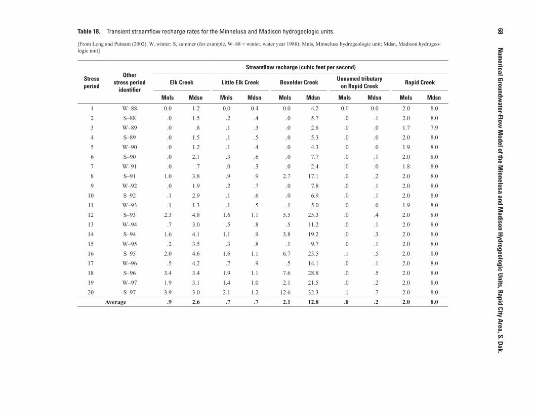
68
Num
erical Groundwater-Flow
Model of the M
innelusa and Madison Hydrogeologic Units, Rapid City Area, S. Dak.
Table 18. Transient streamflow recharge rates for the Minnelusa and Madison hydrogeologic units.
[From Long and Putnam (2002). W, winter; S, summer (for example, W–88 = winter, water year 1988); Mnls, Minnelusa hydrogeologic unit; Mdsn, Madison hydrogeo-logic unit]
Stress period
Other stress period
identifier
Streamflow recharge (cubic feet per second)
Elk Creek Little Elk Creek Boxelder CreekUnnamed tributary
on Rapid CreekRapid Creek
Mnls Mdsn Mnls Mdsn Mnls Mdsn Mnls Mdsn Mnls Mdsn
1 W–88 0.0 1.2 0.0 0.4 0.0 4.2 0.0 0.0 2.0 8.02 S–88 .0 1.5 .2 .4 .0 5.7 .0 .1 2.0 8.03 W–89 .0 .8 .1 .3 .0 2.8 .0 .0 1.7 7.94 S–89 .0 1.5 .1 .5 .0 5.3 .0 .0 2.0 8.05 W–90 .0 1.2 .1 .4 .0 4.3 .0 .0 1.9 8.06 S–90 .0 2.1 .3 .6 .0 7.7 .0 .1 2.0 8.07 W–91 .0 .7 .0 .3 .0 2.4 .0 .0 1.8 8.08 S–91 1.0 3.8 .9 .9 2.7 17.1 .0 .2 2.0 8.09 W–92 .0 1.9 .2 .7 .0 7.8 .0 .1 2.0 8.0
10 S–92 .1 2.9 .1 .6 .0 6.9 .0 .1 2.0 8.011 W–93 .1 1.3 .1 .5 .1 5.0 .0 .0 1.9 8.012 S–93 2.3 4.8 1.6 1.1 5.5 25.3 .0 .4 2.0 8.013 W–94 .7 3.0 .5 .8 .5 11.2 .0 .1 2.0 8.014 S–94 1.6 4.1 1.1 .9 3.8 19.2 .0 .3 2.0 8.015 W–95 .2 3.5 .3 .8 .1 9.7 .0 .1 2.0 8.016 S–95 2.0 4.6 1.6 1.1 6.7 25.5 .1 .5 2.0 8.017 W–96 .5 4.2 .7 .9 .5 14.1 .0 .1 2.0 8.018 S–96 3.4 3.4 1.9 1.1 7.6 28.8 .0 .5 2.0 8.019 W–97 1.9 3.1 1.4 1.0 2.1 21.5 .0 .2 2.0 8.020 S–97 3.9 3.0 2.1 1.2 12.6 32.3 .1 .7 2.0 8.0
Average .9 2.6 .7 .7 2.1 12.8 .0 .2 2.0 8.0

Supplemental Inform
ation
69
Table 18. Transient streamflow recharge rates for the Minnelusa and Madison hydrogeologic units.—Continued
[From Long and Putnam (2002). W, winter; S, summer (for example, W–88 = winter, water year 1988); Mnls, Minnelusa hydrogeologic unit; Mdsn, Madison hydrogeologic unit]
Stress period
Other stress period
identifier
Streamflow recharge (cubic feet per second)
Victoria Creek Spring CreekRockerville
GulchDeadman Gulch Battle Creek
Total of all streams
Total Mnls, MdsnMnls Mdsn Mnls Mdsn Mnls Mdsn Mnls Mdsn Mnls Mdsn Mnls Mdsn
1 W–88 0.0 0.1 0.0 1.1 0.0 0.2 0.0 0.1 0.0 0.3 2.0 15.6 17.62 S–88 .0 .2 .0 2.5 .0 .1 .0 .0 .0 .5 2.2 19.0 21.23 W–89 .0 .0 .0 .2 .0 .1 .0 .0 .0 .2 1.8 12.3 14.14 S–89 .0 .1 .0 1.8 .0 .1 .0 .0 .0 .7 2.1 18.0 20.15 W–90 .0 .1 .0 1.3 .0 .1 .0 .0 .0 1.1 2.0 16.5 18.56 S–90 .0 .9 .9 11.2 .0 .4 .0 .2 .0 4.1 3.2 35.3 38.57 W–91 .0 .2 .0 3.1 .0 .1 .0 .1 .0 .8 1.8 15.7 17.58 S–91 .0 1.4 1.9 16.8 .2 1.2 .1 .6 .0 4.4 8.8 54.4 63.29 W–92 .0 .4 .0 6.7 .0 .3 .0 .1 .0 1.5 2.2 27.5 29.7
10 S–92 .0 .5 .0 8.2 .0 .3 .0 .1 .0 2.3 2.2 29.9 32.111 W–93 .0 .3 .1 4.1 .0 .2 .0 .1 .0 1.1 2.3 20.6 22.912 S–93 .0 1.7 2.6 19.9 .1 1.7 .0 .8 .0 5.7 14.1 69.4 83.513 W–94 .0 .8 .2 11.1 .0 .9 .0 .4 .0 3.3 3.9 39.6 43.514 S–94 .0 .9 .9 11.0 .0 .5 .0 .2 .0 2.1 9.4 47.2 56.615 W–95 .0 .5 .1 7.1 .0 .4 .0 .2 .0 2.0 2.7 32.3 35.016 S–95 .0 1.5 2.1 18.0 .3 2.1 .1 1.1 .0 5.0 14.9 67.4 82.317 W–96 .0 .9 .1 13.1 .0 1.2 .0 .5 .0 3.1 3.8 46.1 49.918 S–96 .0 1.7 2.5 20.3 .1 1.7 .0 .8 .0 5.2 17.5 71.5 89.019 W–97 .0 1.4 1.5 18.5 .0 1.6 .0 .7 .0 4.6 8.9 60.6 69.520 S–97 .0 1.9 3.4 21.0 .2 2.5 .1 1.2 .0 6.0 24.4 77.8 102.2
Average .0 .8 .8 9.9 .0 .8 .0 .4 .0 2.7 6.5 38.8 45.3

70
Num
erical Groundwater-Flow
Model of the M
innelusa and Madison Hydrogeologic Units, Rapid City Area, S. Dak.
Table 19. Transient areal recharge rates for the Minnelusa and Madison hydrogeologic units by zones.
[From Long and Putnam (2002). Areal recharge zones shown in figure 14. W, winter; S, summer (for example, W–88 = winter, water year 1988); Mnls, Minnelusa hydrogeologic unit; Mdsn, Madison hydrogeologic unit]
Stress period
Other stress period
identifier
Areal recharge by zones (cubic feet per second)Total areal recharge
(cubic feet per second)Elk Creek to
Little Elk Creek(Zone 1)
Little Elk Creek toBoxelder Creek
(Zone 2)
Boxelder Creek toRapid Creek
(Zone 3)
Rapid Creek toSpring Creek
(Zone 4)
Spring Creek toBattle Creek
(Zone 5)
Mnls Mdsn Mnls Mdsn Mnls Mdsn Mnls Mdsn Mnls Mdsn Mnls MdsnMnls, Mdsn
1 W–88 0.1 0.5 0.1 0.3 0.0 0.3 0.0 0.0 0.0 0.0 0.2 0.9 1.1
2 S–88 .1 .9 .1 .6 .1 .6 .0 .1 .2 .2 .5 1.9 2.4
3 W–89 .1 .5 .2 .6 .2 .6 .0 .1 .1 .1 .6 1.6 2.2
4 S–89 .3 2.4 .9 3.1 1.0 3.1 .8 1.6 1.0 .9 4.0 10.0 14.0
5 W–90 .2 1.5 .3 1.1 .2 1.1 .1 .1 .2 .2 1.0 3.2 4.2
6 S–90 .1 .9 .7 2.2 .6 2.2 .5 .8 2.2 2.3 4.1 7.4 11.5
7 W–91 .1 .8 .2 .6 .1 .6 .0 .1 .1 .1 .5 1.8 2.3
8 S–91 1.3 7.5 6.4 24.0 4.9 24.0 2.6 5.5 4.3 4.5 19.5 52.5 72.0
9 W–92 .1 .9 .2 .8 .1 .8 .1 .1 .3 .3 .8 2.4 3.2
10 S–92 .2 1.0 .9 3.1 .4 3.1 .2 .4 .6 .5 2.3 5.9 8.2
11 W–93 .1 1.1 .2 .7 .1 .7 .0 .1 .1 .1 .5 2.2 2.7
12 S–93 1.7 10.0 5.3 19.6 3.5 19.6 2.3 4.0 7.1 6.2 19.9 46.0 65.9
13 W–94 .2 1.8 .2 .8 .1 .8 .0 .0 .0 .1 .5 2.9 3.4
14 S–94 .1 .4 .3 .8 .1 .8 .1 .1 .4 .4 1.0 2.0 3.0
15 W–95 .4 3.1 .6 2.4 .3 2.4 .0 .1 .2 .3 1.5 6.5 8.0
16 S–95 2.9 18.4 11.6 35.8 4.6 35.8 1.1 2.1 5.5 5.5 25.7 72.7 98.4
17 W–96 .3 2.8 .5 2.2 .2 2.2 .1 .1 .2 .2 1.3 5.8 7.1
18 S–96 1.1 4.5 4.4 17.8 2.1 17.8 .9 1.5 3.0 3.0 11.5 31.1 42.6
19 W–97 .6 2.6 1.2 4.8 .7 4.8 .2 .4 .5 .5 3.2 9.6 12.8
20 S–97 1.4 5.8 11.6 35.0 5.9 35.0 1.1 1.8 3.3 3.1 23.3 56.3 79.6
Average .6 3.4 2.3 7.8 1.3 7.8 .5 1.0 1.5 1.4 6.1 16.1 22.2

Supplemental Information 71
Table 20. Observed and simulated hydraulic head values for the Minnelusa hydrogeologic unit in steady-state simulation. —Continued
[Observation name corresponds to site number in table 29 and plate 2 of Long and Putnam (2002). Observed hydraulic head from Long and Putnam (2002). Implied accuracy is standard deviation of measurement error (SDME), which is used in the parameter estimation process to weight observations (weight = 1/(SDME)2) (Hill and others, 2000). Implied accuracy for sites with a single measurement was assigned a value of 10. Implied accuracy for sites with time-series measurements was assigned a value of 1. Implied accuracy for sites with multiple measurements was assigned a value of 5. Other identifier used in Long and Putnam (2002). NGVD 29, National Geodetic Vertical Datum of 1929; --, none]
Observation name and
site number
Model cell location
Observed hydraulic
head (feet above
NGVD 29)
Simulated hydraulic
head(feet above NGVD 29)
Difference between simlated
and observed hydraulic
head (feet)
Implied accuracy of
hydraulic head
(feet)
Station identification
number
Other identifierLayer Row Column
102 1 2 89 3,454 3,486 32 10 441812103230501 --103 1 1 75 3,564 3,574 10 10 441826103263301 --104 1 1 70 3,610 3,602 -8 1 441759103261201 TF–1105 1 5 74 3,515 3,573 58 10 441701103251101 PDMT-East106 1 4 65 3,592 3,653 61 10 441656103261601 --107 1 4 65 3,593 3,652 59 10 441649103262401 --108 1 6 65 3,529 3,624 95 10 441620103255301 --109 1 7 68 3,532 3,591 59 10 441612103252801 --110 1 8 68 3,557 3,586 29 10 441606103252501 --111 1 8 66 3,514 3,591 77 10 441556103253201 --112 1 13 79 3,428 3,486 58 10 441504103230301 --113 1 13 74 3,422 3,524 102 10 441500103240601 --114 1 13 69 3,486 3,563 77 10 441453103243801 --115 1 12 66 3,527 3,582 55 10 442221103245501 --116 1 16 83 3,412 3,458 46 10 441314103233301 --117 1 14 67 3,506 3,583 77 10 441424103243601 --118 1 15 68 3,510 3,576 66 10 441421103242302 --119 1 17 79 3,478 3,491 13 10 441400103231501 --120 1 16 67 3,526 3,594 68 10 441358103241801 --121 1 18 73 3,490 3,547 57 10 441643103232801 --122 1 18 73 3,530 3,550 20 10 441339103232701 --123 1 18 72 3,528 3,557 29 10 441338103233201 --124 1 19 78 3,481 3,508 27 1 441337103225001 PDMT–1125 1 19 80 3,414 3,487 73 10 441335103223202 --126 1 19 80 3,414 3,487 73 10 441335103223201 --127 1 19 81 3,457 3,483 26 10 441333103222801 --128 1 19 75 3,454 3,531 77 10 441331103230701 --129 2 19 69 3,547 3,690 143 10 441322103234202 --130 2 19 69 3,581 3,669 88 10 441322103234201 --131 1 20 78 3,489 3,497 8 10 441315103224001 --132 1 21 78 3,458 3,492 34 10 441257103222501 --133 1 26 109 3,268 3,278 10 10 441241103183401 --134 1 25 89 3,414 3,418 4 10 441219103204801 --135 1 24 79 3,495 3,499 4 10 441242103215701 --136 1 24 79 3,477 3,499 22 10 441216103215801 --

72 Numerical Groundwater-Flow Model of the Minnelusa and Madison Hydrogeologic Units, Rapid City Area, S. Dak.
Table 20. Observed and simulated hydraulic head values for the Minnelusa hydrogeologic unit in steady-state simulation. —Continued
[Observation name corresponds to site number in table 29 and plate 2 of Long and Putnam (2002). Observed hydraulic head from Long and Putnam (2002). Implied accuracy is standard deviation of measurement error (SDME), which is used in the parameter estimation process to weight observations (weight = 1/(SDME)2) (Hill and others, 2000). Implied accuracy for sites with a single measurement was assigned a value of 10. Implied accuracy for sites with time-series measurements was assigned a value of 1. Implied accuracy for sites with multiple measurements was assigned a value of 5. Other identifier used in Long and Putnam (2002). NGVD 29, National Geodetic Vertical Datum of 1929; --, none]
Observation name and
site number
Model cell location
Observed hydraulic
head (feet above
NGVD 29)
Simulated hydraulic
head(feet above NGVD 29)
Difference between simlated
and observed hydraulic
head (feet)
Implied accuracy of
hydraulic head
(feet)
Station identification
number
Other identifierLayer Row Column
137 1 25 81 3,483 3,488 5 10 441210103215101 --138 1 26 93 3,366 3,393 27 10 441212103201501 --139 1 25 81 3,458 3,483 25 10 441211103213701 --140 1 25 84 3,476 3,462 -14 10 441202103211301 --141 1 26 90 3,449 3,412 -37 10 441318103221301 --142 1 25 81 3,444 3,489 45 10 442137103213801 --143 1 25 81 3,474 3,485 11 10 441202103213301 --144 1 26 81 3,471 3,483 12 10 441200103213001 --145 1 26 84 3,445 3,465 20 10 441157103213701 --146 1 26 80 3,451 3,490 39 10 441220103214001 --147 1 26 82 3,459 3,479 20 10 441151103213002 --148 1 29 95 3,413 3,388 -25 10 441147103270001 --149 2 27 80 3,415 3,581 166 10 441136103221301 --150 1 27 81 3,460 3,485 25 10 441134103211601 --151 1 29 91 3,418 3,416 -2 10 441131103200101 --152 1 28 84 3,466 3,467 1 10 441130103205601 --153 1 28 82 3,453 3,480 27 10 441119103210301 --154 1 31 95 3,454 3,398 -56 10 441105103192001 --155 1 30 86 3,413 3,462 49 10 441125103203001 --156 1 30 83 3,403 3,482 79 10 441038103203001 --157 1 31 83 3,423 3,479 56 10 441049103203701 --158 1 31 84 3,423 3,474 51 10 441047103203301 --159 2 31 82 3,496 3,588 92 10 441323103232301 --160 1 31 83 3,438 3,477 39 10 441040103203201 --161 1 31 83 3,492 3,476 -16 10 441038103203002 --162 2 31 83 3,472 3,583 111 10 441037103203502 --163 2 31 83 3,450 3,583 133 10 441037103203501 --164 1 33 91 3,463 3,433 -30 10 441033103193001 --165 1 32 88 3,443 3,449 6 10 441031103195201 --166 1 32 85 3,487 3,464 -23 10 441024103201301 --167 2 32 81 3,474 3,604 130 10 441023103204001 --168 2 32 82 3,440 3,593 153 10 441023103203101 --169 2 32 82 3,423 3,590 167 10 441023103203001 --170 1 33 84 3,432 3,474 42 10 441007103201101 --171 1 39 100 3,489 3,439 -50 10 440930103175201 --

Supplemental Information 73
Table 20. Observed and simulated hydraulic head values for the Minnelusa hydrogeologic unit in steady-state simulation. —Continued
[Observation name corresponds to site number in table 29 and plate 2 of Long and Putnam (2002). Observed hydraulic head from Long and Putnam (2002). Implied accuracy is standard deviation of measurement error (SDME), which is used in the parameter estimation process to weight observations (weight = 1/(SDME)2) (Hill and others, 2000). Implied accuracy for sites with a single measurement was assigned a value of 10. Implied accuracy for sites with time-series measurements was assigned a value of 1. Implied accuracy for sites with multiple measurements was assigned a value of 5. Other identifier used in Long and Putnam (2002). NGVD 29, National Geodetic Vertical Datum of 1929; --, none]
Observation name and
site number
Model cell location
Observed hydraulic
head (feet above
NGVD 29)
Simulated hydraulic
head(feet above NGVD 29)
Difference between simlated
and observed hydraulic
head (feet)
Implied accuracy of
hydraulic head
(feet)
Station identification
number
Other identifierLayer Row Column
172 1 37 87 3,447 3,460 13 10 440936103191801 Blackhawk Water Co. No. 3
173 1 42 106 3,416 3,402 -14 10 440919103170501 --174 1 44 110 3,379 3,372 -7 10 440929103163501 --175 1 45 110 3,392 3,379 -13 10 440916103163301 --176 1 40 92 3,386 3,457 71 10 440907103183501 Blackhawk
Water Co. No. 2
177 1 38 83 3,462 3,467 5 10 440908103193101 --178 1 40 90 3,403 3,460 57 10 440901103184801 Blackhawk
Water Co. No. 1
179 1 47 89 3,414 3,461 47 10 440829103183801 --180 1 50 96 3,410 3,450 40 10 440826103174601 --181 1 50 92 3,422 3,456 34 1 440818103180801 BLHK–1182 1 50 91 3,449 3,457 8 10 440818103174701 --183 1 59 104 3,313 3,430 117 10 440800103163001 --184 1 60 93 3,409 3,450 41 10 440738103173901 --185 1 60 93 3,412 3,450 38 10 440736103173701 --186 1 63 90 3,434 3,453 19 10 440719103174801 --187 1 79 107 3,400 3,385 -15 10 440636103152001 --188 1 77 99 3,420 3,418 -2 10 440635103161801 --189 1 82 102 3,383 3,399 16 10 440607103155901 --190 1 77 85 3,419 3,445 26 10 440606103174701 --191 1 77 86 3,419 3,442 23 10 440605103174701 --192 1 77 84 3,421 3,445 24 10 440552103173401 --193 1 77 85 3,427 3,443 16 10 440603103174501 --194 1 82 95 3,336 3,412 76 10 440552103162301 --195 1 79 85 3,414 3,441 27 10 440557103174401 --196 1 79 84 3,449 3,443 -6 10 440556103174801 --197 1 80 87 3,410 3,433 23 10 440542103172501 --198 1 80 85 3,443 3,437 -6 10 440639103173701 --199 1 81 85 3,438 3,434 -4 10 440545103173501 --200 1 80 81 3,450 3,448 -2 1 440544103180001 CQ–1201 1 81 84 3,444 3,437 -7 10 440544103174301 --

74 Numerical Groundwater-Flow Model of the Minnelusa and Madison Hydrogeologic Units, Rapid City Area, S. Dak.
Table 20. Observed and simulated hydraulic head values for the Minnelusa hydrogeologic unit in steady-state simulation. —Continued
[Observation name corresponds to site number in table 29 and plate 2 of Long and Putnam (2002). Observed hydraulic head from Long and Putnam (2002). Implied accuracy is standard deviation of measurement error (SDME), which is used in the parameter estimation process to weight observations (weight = 1/(SDME)2) (Hill and others, 2000). Implied accuracy for sites with a single measurement was assigned a value of 10. Implied accuracy for sites with time-series measurements was assigned a value of 1. Implied accuracy for sites with multiple measurements was assigned a value of 5. Other identifier used in Long and Putnam (2002). NGVD 29, National Geodetic Vertical Datum of 1929; --, none]
Observation name and
site number
Model cell location
Observed hydraulic
head (feet above
NGVD 29)
Simulated hydraulic
head(feet above NGVD 29)
Difference between simlated
and observed hydraulic
head (feet)
Implied accuracy of
hydraulic head
(feet)
Station identification
number
Other identifierLayer Row Column
202 1 82 85 3,468 3,434 -34 10 440544103173601 --205 1 87 96 3,328 3,395 67 10 440538103161001 --206 1 83 82 3,467 3,435 -32 10 440534103174801 --207 1 85 87 3,450 3,421 -29 10 440534103171401 --209 1 89 95 3,412 3,396 -16 1 440528103161001 CP210 1 90 98 3,406 3,391 -15 10 440528103155201 --211 1 82 74 3,471 3,442 -29 10 440521103184401 --212 1 85 78 3,462 3,428 -34 10 440532103182001 --213 1 92 94 3,403 3,393 -10 10 440514103161401 --214 1 85 76 3,434 3,430 -4 10 450512103182101 --215 2 83 65 3,406 3,478 72 10 440516103194001 WT–1216 1 88 76 3,475 3,422 -53 10 440501103181501 --217 1 88 77 3,450 3,419 -31 10 440459103181001 --218 1 88 76 3,450 3,419 -31 10 440458103181101 --219 1 97 95 3,396 3,383 -13 10 440452103155301 South Dakota
ARNG220 1 90 75 3,435 3,415 -20 10 440449103181501 --221 1 90 75 3,415 3,414 -1 10 440446103181801 --222 1 91 75 3,470 3,413 -57 10 440445103181601 --223 1 101 92 3,392 3,375 -17 1 440430103160201 SP–1224 1 95 74 3,400 3,399 -1 1 440423103180501 WCR–3225 1 97 69 3,382 3,400 18 10 440403103183701 --226 2 99 64 3,435 3,451 16 10 440347103190501 --227 2 99 63 3,456 3,452 -4 10 440344103190801 --228 1 104 75 3,360 3,373 13 10 440344103173701 --229 1 106 75 3,360 3,369 9 1 440338103173301 CL–1230 1 113 89 3,396 3,363 -33 10 440331103155101 --231 1 106 70 3,395 3,384 -11 5 440326103180703 JS–1B232 1 107 69 3,365 3,385 20 10 440321103181001 --233 1 110 72 3,383 3,378 -5 1 440310103173801 CHLN–1234 1 113 78 3,360 3,376 16 10 440309103170101 --235 2 108 65 3,435 3,461 26 10 440308103183001 --236 1 112 74 3,378 3,377 -1 10 440308103172501 --237 1 121 97 3,353 3,325 -28 10 440308103144301 --238 1 112 74 3,353 3,378 25 10 440336103165301 --

Supplemental Information 75
Table 20. Observed and simulated hydraulic head values for the Minnelusa hydrogeologic unit in steady-state simulation. —Continued
[Observation name corresponds to site number in table 29 and plate 2 of Long and Putnam (2002). Observed hydraulic head from Long and Putnam (2002). Implied accuracy is standard deviation of measurement error (SDME), which is used in the parameter estimation process to weight observations (weight = 1/(SDME)2) (Hill and others, 2000). Implied accuracy for sites with a single measurement was assigned a value of 10. Implied accuracy for sites with time-series measurements was assigned a value of 1. Implied accuracy for sites with multiple measurements was assigned a value of 5. Other identifier used in Long and Putnam (2002). NGVD 29, National Geodetic Vertical Datum of 1929; --, none]
Observation name and
site number
Model cell location
Observed hydraulic
head (feet above
NGVD 29)
Simulated hydraulic
head(feet above NGVD 29)
Difference between simlated
and observed hydraulic
head (feet)
Implied accuracy of
hydraulic head
(feet)
Station identification
number
Other identifierLayer Row Column
239 1 109 67 3,399 3,389 -10 10 440307103181501 --240 1 114 78 3,364 3,377 13 10 440305103164501 --241 1 115 78 3,370 3,377 7 10 440211103165601 --242 1 115 78 3,350 3,378 28 10 440301103165701 --243 1 114 76 3,380 3,378 -2 10 440300103170901 --244 1 115 75 3,355 3,379 24 10 440257103171101 --245 1 115 74 3,336 3,381 45 10 440252103172201 --246 2 112 65 3,450 3,467 17 10 440249103182101 --247 1 117 75 3,342 3,381 39 10 440247103165401 --248 1 118 75 3,386 3,382 -4 10 440242103170801 --249 1 121 82 3,374 3,378 4 10 440244103154102 --250 1 126 92 3,351 3,341 -10 10 440236103145801 --251 1 120 74 3,387 3,384 -3 10 440233103170501 --252 1 123 81 3,381 3,381 0 5 440223103161701 Springbrook
West Well No. 2
253 2 120 71 3,372 3,439 67 10 440224103172601 Carriage Hills No. 2
254 1 126 86 3,388 3,368 -20 5 440214103153501 Springbrook East Well
255 1 124 73 3,401 3,388 -13 10 440211103165201 --256 1 125 76 3,409 3,387 -22 10 440211103164301 --257 1 132 89 3,392 3,348 -44 10 440204103150001 --258 1 134 93 3,390 3,335 -55 10 440203103143601 --259 1 131 80 3,429 3,390 -39 5 440158103160401 Springbrook
South No. 3
260 1 129 73 3,412 3,406 -6 1 440149103164901 Wildwood North
261 1 134 73 3,429 3,423 -6 5 440130103163401 Wildwood South
262 1 144 86 3,376 3,360 -16 10 440103103144801 --263 1 145 82 3,456 3,396 -60 10 440059103154101 --264 1 147 85 3,455 3,377 -78 10 440048103145001 --265 1 141 63 3,475 3,485 10 10 440038103172601 --266 1 145 70 3,459 3,469 10 10 440031103162701 --

76 Numerical Groundwater-Flow Model of the Minnelusa and Madison Hydrogeologic Units, Rapid City Area, S. Dak.
Table 20. Observed and simulated hydraulic head values for the Minnelusa hydrogeologic unit in steady-state simulation. —Continued
[Observation name corresponds to site number in table 29 and plate 2 of Long and Putnam (2002). Observed hydraulic head from Long and Putnam (2002). Implied accuracy is standard deviation of measurement error (SDME), which is used in the parameter estimation process to weight observations (weight = 1/(SDME)2) (Hill and others, 2000). Implied accuracy for sites with a single measurement was assigned a value of 10. Implied accuracy for sites with time-series measurements was assigned a value of 1. Implied accuracy for sites with multiple measurements was assigned a value of 5. Other identifier used in Long and Putnam (2002). NGVD 29, National Geodetic Vertical Datum of 1929; --, none]
Observation name and
site number
Model cell location
Observed hydraulic
head (feet above
NGVD 29)
Simulated hydraulic
head(feet above NGVD 29)
Difference between simlated
and observed hydraulic
head (feet)
Implied accuracy of
hydraulic head
(feet)
Station identification
number
Other identifierLayer Row Column
267 1 147 73 3,412 3,458 46 10 440028103160801 --268 1 147 72 3,499 3,460 -39 10 440027103161001 --269 1 146 69 3,494 3,478 -16 10 440022103163401 --270 1 148 69 3,455 3,480 25 10 440007103165301 --271 1 152 75 3,404 3,448 44 10 440010103154201 --272 1 160 65 3,493 3,473 -20 1 435916103161802 RG–2273 1 164 67 3,476 3,466 -10 10 435858103155701 --274 1 175 62 3,539 3,449 -90 10 435803103160301 --275 1 177 58 3,548 3,447 -101 10 445809103162201 --276 1 183 75 3,547 3,414 -133 10 435720103141601 Hart Ranch
No. 3277 1 193 36 3,558 3,456 -102 10 435352103170801 --278 2 196 27 3,527 3,514 -13 10 435325103171701 --279 1 199 25 3,551 3,467 -84 10 435225103172801 --280 1 203 17 3,536 3,504 -32 10 435119103175001 --
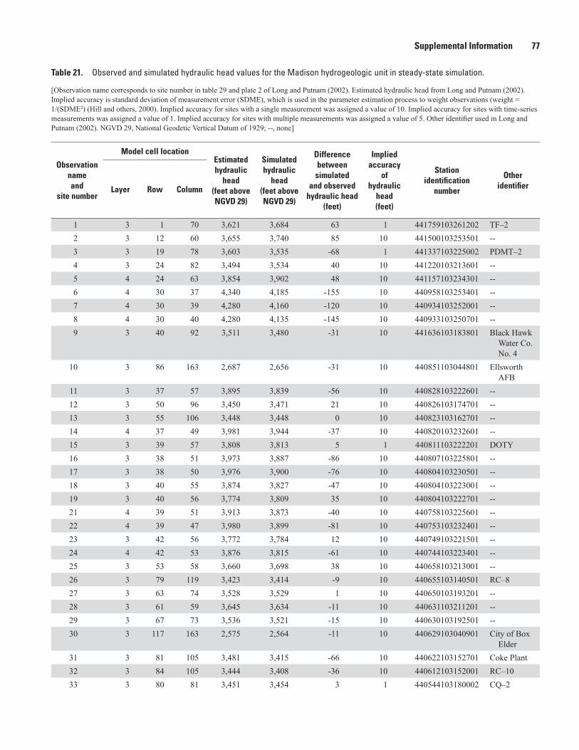
Supplemental Information 77
Table 21. Observed and simulated hydraulic head values for the Madison hydrogeologic unit in steady-state simulation. —Continued
[Observation name corresponds to site number in table 29 and plate 2 of Long and Putnam (2002). Estimated hydraulic head from Long and Putnam (2002). Implied accuracy is standard deviation of measurement error (SDME), which is used in the parameter estimation process to weight observations (weight = 1/(SDME2) (Hill and others, 2000). Implied accuracy for sites with a single measurement was assigned a value of 10. Implied accuracy for sites with time-series measurements was assigned a value of 1. Implied accuracy for sites with multiple measurements was assigned a value of 5. Other identifier used in Long and Putnam (2002). NGVD 29, National Geodetic Vertical Datum of 1929; --, none]
Observation name and
site number
Model cell locationEstimated hydraulic
head(feet above NGVD 29)
Simulated hydraulic
head(feet above NGVD 29)
Difference between simulated
and observed hydraulic head
(feet)
Implied accuracy
of hydraulic
head (feet)
Station identification
number
OtheridentifierLayer Row Column
1 3 1 70 3,621 3,684 63 1 441759103261202 TF–22 3 12 60 3,655 3,740 85 10 441500103253501 --3 3 19 78 3,603 3,535 -68 1 441337103225002 PDMT–24 3 24 82 3,494 3,534 40 10 441220103213601 --5 4 24 63 3,854 3,902 48 10 441157103234301 --6 4 30 37 4,340 4,185 -155 10 440958103253401 --7 4 30 39 4,280 4,160 -120 10 440934103252001 --8 4 30 40 4,280 4,135 -145 10 440933103250701 --9 3 40 92 3,511 3,480 -31 10 441636103183801 Black Hawk
Water Co. No. 4
10 3 86 163 2,687 2,656 -31 10 440851103044801 Ellsworth AFB
11 3 37 57 3,895 3,839 -56 10 440828103222601 --12 3 50 96 3,450 3,471 21 10 440826103174701 --13 3 55 106 3,448 3,448 0 10 440823103162701 --14 4 37 49 3,981 3,944 -37 10 440820103232601 --15 3 39 57 3,808 3,813 5 1 440811103222201 DOTY16 3 38 51 3,973 3,887 -86 10 440807103225801 --17 3 38 50 3,976 3,900 -76 10 440804103230501 --18 3 40 55 3,874 3,827 -47 10 440804103223001 --19 3 40 56 3,774 3,809 35 10 440804103222701 --21 4 39 51 3,913 3,873 -40 10 440758103225601 --22 4 39 47 3,980 3,899 -81 10 440753103232401 --23 3 42 56 3,772 3,784 12 10 440749103221501 --24 4 42 53 3,876 3,815 -61 10 440744103223401 --25 3 53 58 3,660 3,698 38 10 440658103213001 --26 3 79 119 3,423 3,414 -9 10 440655103140501 RC–827 3 63 74 3,528 3,529 1 10 440650103193201 --28 3 61 59 3,645 3,634 -11 10 440631103211201 --29 3 67 73 3,536 3,521 -15 10 440630103192501 --30 3 117 163 2,575 2,564 -11 10 440629103040901 City of Box
Elder31 3 81 105 3,481 3,415 -66 10 440622103152701 Coke Plant32 3 84 105 3,444 3,408 -36 10 440612103152001 RC–1033 3 80 81 3,451 3,454 3 1 440544103180002 CQ–2

78 Numerical Groundwater-Flow Model of the Minnelusa and Madison Hydrogeologic Units, Rapid City Area, S. Dak.
Table 21. Observed and simulated hydraulic head values for the Madison hydrogeologic unit in steady-state simulation. —Continued
[Observation name corresponds to site number in table 29 and plate 2 of Long and Putnam (2002). Estimated hydraulic head from Long and Putnam (2002). Implied accuracy is standard deviation of measurement error (SDME), which is used in the parameter estimation process to weight observations (weight = 1/(SDME2) (Hill and others, 2000). Implied accuracy for sites with a single measurement was assigned a value of 10. Implied accuracy for sites with time-series measurements was assigned a value of 1. Implied accuracy for sites with multiple measurements was assigned a value of 5. Other identifier used in Long and Putnam (2002). NGVD 29, National Geodetic Vertical Datum of 1929; --, none]
Observation name and
site number
Model cell locationEstimated hydraulic
head(feet above NGVD 29)
Simulated hydraulic
head(feet above NGVD 29)
Difference between simulated
and observed hydraulic head
(feet)
Implied accuracy
of hydraulic
head (feet)
Station identification
number
OtheridentifierLayer Row Column
34 3 70 55 3,646 3,581 -65 10 440540103211301 --35 3 85 84 3,447 3,425 -22 10 440526103173001 RC–636 3 91 97 3,424 3,404 -20 10 440523103155701 BHPL37 3 80 67 3,477 3,509 32 10 440518103193001 --38 4 73 46 3,734 3,694 -40 10 440512103215701 --39 4 73 45 3,764 3,716 -48 10 440508103220701 --40 3 83 63 3,520 3,513 -7 10 440500103193601 WT–241 3 88 72 3,405 3,432 27 10 440453103184001 --42 3 86 64 3,430 3,468 38 10 440446103193201 --43 3 97 91 3,417 3,402 -15 10 440446103161701 LC44 3 87 64 3,428 3,456 28 10 440441103193301 --45 3 90 66 3,405 3,417 12 10 440432103191401 --46 3 101 91 3,423 3,401 -22 1 440430103160202 SP–247 3 110 114 3,146 3,198 52 1 440427103131701 RC–748 3 99 62 3,418 3,416 -2 10 440337103191801 --49 3 110 87 3,415 3,396 -19 10 440342103160701 RC–950 3 106 75 3,418 3,405 -13 1 440338103173302 CL–251 3 132 138 2,655 2,584 -71 10 440334103095601 Rapid Valley
No. 4, RV–4
52 3 106 70 3,418 3,402 -16 1 440326103180702 JS–1A53 3 110 73 3,418 3,406 -12 10 440310103173802 CHLN–354 3 107 63 3,417 3,415 -2 1 440308103184601 CLEGmdsn55 3 110 69 3,419 3,405 -14 10 440308103180701 --

Supplemental Information 79
Table 21. Observed and simulated hydraulic head values for the Madison hydrogeologic unit in steady-state simulation. —Continued
[Observation name corresponds to site number in table 29 and plate 2 of Long and Putnam (2002). Estimated hydraulic head from Long and Putnam (2002). Implied accuracy is standard deviation of measurement error (SDME), which is used in the parameter estimation process to weight observations (weight = 1/(SDME2) (Hill and others, 2000). Implied accuracy for sites with a single measurement was assigned a value of 10. Implied accuracy for sites with time-series measurements was assigned a value of 1. Implied accuracy for sites with multiple measurements was assigned a value of 5. Other identifier used in Long and Putnam (2002). NGVD 29, National Geodetic Vertical Datum of 1929; --, none]
Observation name and
site number
Model cell locationEstimated hydraulic
head(feet above NGVD 29)
Simulated hydraulic
head(feet above NGVD 29)
Difference between simulated
and observed hydraulic head
(feet)
Implied accuracy
of hydraulic
head (feet)
Station identification
number
OtheridentifierLayer Row Column
56 3 112 72 3,419 3,408 -11 10 440300103173501 CHLN–257 3 108 61 3,415 3,419 4 10 440247103192401 --58 3 107 56 3,438 3,427 -11 10 440302103194601 --59 3 110 57 3,434 3,426 -8 10 440247103191701 --60 3 113 60 3,416 3,422 6 10 440238103185201 --61 3 120 70 3,426 3,420 -6 10 440223103173201 Carriage
Hills No. 1, CH
62 3 124 77 3,423 3,422 -1 10 440220103164001 RC–1163 3 124 70 3,445 3,426 -19 10 440205103172001 --64 3 137 62 3,475 3,463 -12 10 440054103173801 --65 4 137 43 3,806 3,626 -180 10 440523103194201 --66 3 146 58 3,531 3,543 12 10 440004103174001 HH67 4 148 48 3,626 3,639 13 10 435937103184101 --68 3 160 65 3,497 3,511 14 1 435916103161801 RG69 4 156 49 3,594 3,617 23 10 435903103181301 --70 4 157 44 3,580 3,639 59 10 435851103184201 --71 3 170 77 3,498 3,476 -22 10 435851103143501 HR–272 3 176 55 3,488 3,514 26 10 435746103160601 --73 3 187 84 3,498 3,375 -123 10 435718103130301 HR–174 3 183 38 3,515 3,552 37 10 435635103181401 PG75 3 187 52 3,509 3,481 -28 10 435619103161901 --76 3 189 38 3,530 3,509 -21 10 435518103173001 --77 3 198 13 3,542 3,620 78 10 435227103185301 HWRD

80 Numerical Groundwater-Flow Model of the Minnelusa and Madison Hydrogeologic Units, Rapid City Area, S. Dak.
Table 22. Supplemental interpolated hydraulic head values for the Minnelusa and Madison hydrogeologic units in steady-state simulation. —Continued
[Interpolated hydraulic head from estimated potentiometric contours in Long and Putnam (2002, plates 1 and 2). Implied accuracy is standard deviation of mea-surement error (SDME), which is used in the parameter estimation process to weight observations (weight = 1/(SDME)2 (Hill and others, 2000). The SDME or implied accuracy for these supplemental sites was set at 10 feet. NGVD 29, National Geodetic Vertical Datum of 1929]
Observation name
Model cell location
Interpolated hydraulic head
(feet above NGVD 29)
Simulated hydraulic head
(feet above NGVD 29)
Difference between
simulated and interpolated
hydraulic head (feet)
Implied accuracy of
hydraulic head (feet)
Layer Row Column
Minnelusa hydrogeologic unit
801 1 17 162 3,020 3,001 -19 10802 1 11 102 3,315 3,382 67 10803 1 21 152 3,160 3,131 -29 10804 1 34 128 3,266 3,197 -69 10805 1 34 164 2,880 2,849 -31 10806 1 69 156 3,070 3,010 -60 10807 1 176 133 3,100 3,094 -6 10808 1 193 163 2,780 2,816 36 10809 1 193 139 3,130 3,043 -87 10810 1 195 90 3,430 3,269 -161 10811 1 122 126 3,150 3,184 34 10812 1 76 161 2,900 2,890 -10 10813 1 184 157 2,900 2,927 27 10814 1 128 159 2,800 2,903 103 10815 1 139 115 3,200 3,225 25 10816 1 212 157 3,105 2,953 -152 10817 1 104 124 3,200 3,227 27 10818 1 127 154 2,900 3,006 106 10819 1 122 142 3,000 3,093 93 10820 1 162 141 3,000 3,063 63 10

Supplemental Information 81
Table 22. Supplemental interpolated hydraulic head values for the Minnelusa and Madison hydrogeologic units in steady-state simulation. —Continued
[Interpolated hydraulic head from estimated potentiometric contours in Long and Putnam (2002, plates 1 and 2). Implied accuracy is standard deviation of mea-surement error (SDME), which is used in the parameter estimation process to weight observations (weight = 1/(SDME)2 (Hill and others, 2000). The SDME or implied accuracy for these supplemental sites was set at 10 feet. NGVD 29, National Geodetic Vertical Datum of 1929]
Observation name
Model cell location
Interpolated hydraulic head
(feet above NGVD 29)
Simulated hydraulic head
(feet above NGVD 29)
Difference between
simulated and interpolated
hydraulic head (feet)
Implied accuracy of
hydraulic head (feet)
Layer Row Column
Madison hydrogeologic unit
901 3 17 162 3,010 2,989 -21 10902 3 11 102 3,300 3,399 99 10903 3 21 152 3,100 3,126 26 10904 3 34 128 3,200 3,208 8 10905 3 34 164 2,880 2,792 -88 10906 3 69 156 3,050 2,822 -228 10907 3 176 133 2,900 2,854 -46 10908 3 193 163 2,775 2,708 -67 10909 3 193 139 3,090 2,973 -117 10910 3 195 90 3,400 3,266 -134 10911 3 122 126 2,910 2,914 4 10912 3 76 161 2,880 2,724 -156 10913 3 184 157 2,710 2,700 -10 10914 3 128 159 2,570 2,588 18 10915 3 139 115 3,020 3,038 18 10916 3 212 157 3,100 2,897 -203 10917 3 104 124 3,100 3,127 27 10918 3 127 154 2,600 2,604 4 10919 3 122 142 2,700 2,623 -77 10920 3 162 141 2,700 2,648 -52 10

Publishing support provided by:Helena Publishing Service Center
For more information concerning this publication, contact:Director, USGS South Dakota Water Science Center1608 Mt. View Rd.Rapid City, SD 57702(605) 394–3200
Or visit the South Dakota Water Science Center Web site at:http://sd.water.usgs.gov


Printed on recycled paper
Putnam and Long—
Num
erical Groundw
ater-Flow M
odel of the Minnelusa and M
adison Hydrogeologic U
nits, Rapid City Area, South D
akota—SIR 2009–5205


![Data Validation Charts for Aerosol Sulfate Definitions: Sulfate concentration: SO4fVal = [SO4]](https://img.pdfslide.us/doc/110x75/5681474d550346895db491a6/data-validation-charts-for-aerosol-sulfate-definitions-sulfate-concentration-5697209c43453.jpg)