NUMERICAL EXPERIMENTS IN REVISITED BRITTLE FRACTURE.

B. Bourdin G. A. Francfort

J.-J. Marigo∗

Institut Galilee, Universite Paris-Nord, 93430 Villetaneuse, France

Abstract

The numerical implementation of the model of brittle fracture developed in Francfort

and Marigo (1998) is presented. Various computational methods based on variational

approximations of the original functional are proposed. They are tested on several an-

tiplanar and planar examples that are beyond the reach of the classical computational

tools of fracture mechanics.

Keywords : fracture, fracture toughness, energy methods, variational calculus, finite

elements.

1 Introduction

The present work follows in the footsteps of a previous study (Francfort and Marigo, 1998)

where a variational model for quasistatic crack evolution in a brittle material is proposed.

Its merits and drawbacks are elaborated upon in Francfort and Marigo (1998) and we will

presently refrain from any further commenting, so as to concentrate instead on a numerical

feasibility study. Our goal is to convince the reader that the model lives up to its theoretical

expectation and is a useful and manageable predictive tool. To this end, we will confront

settings that are beyond the scope of the usual computational arsenal of the investigator in

the field; we will demonstrate that a carefully tailored numerical version of the model does

not stall in such hostile environments but delivers cracks evolutions which fit squarely within

the proposed framework.

Of course, we still fall short of the ultimate goal of any predictive theory, namely the

corroboration and prediction of experimental results. Such a goal cannot be contemplated

without prior internal review of the self-consistency of the model. This is how the present

work should be viewed, although we do not turn a blind eye to experimental results, whenever

they are known to us. But, in all fairness, such comparisons can only be qualitative in the

absence of a detailed experimental/numerical protocol. We do hope to be able, in a not too

distant future, to report on the success —or failure— of such an undertaking.

Let us now briefly recapitulate the main features of the model in an exemplary setting: a

homogeneous two-dimensional elastic body Ω with elasticity tensor A and fracture toughness

∗To whom correspondence should be addressed. e-Mail : marigo@lpmtm.univ-paris13.fr

1

k is submitted to an imposed displacement field U(t, x) on the part ∂Ω \ N of its boundary

and free of tractions on the complementary part N of that boundary. We further assume

that, at time t = 0, the body Ω is uncracked and that U(t, x) = tU(x), where U(x) is

a smooth displacement field. If Γ is a crack, a compact in Ω (the crack may go to the

boundary), its surface energy is

Es(Γ) = kH1(Γ \ N ),

where, here and in the remainder of the paper, Hn−1 denotes the n−1–dimensional Hausdorff

measure, a measure which coincides with the usual surface measure for smooth enough

hypersurfaces of Rn. Note that the surface energy will be infinite for cracks that are too

fat, i.e., with infinite one-dimensional Hausdorff measure. Note also that this definition of

the surface energy slightly departs from that proposed in Francfort and Marigo (1998); the

resulting formulation will however be equivalent.

We now define the bulk energy as

Ee(Γ, t) = infw

∫

Ω\ΓAe(w) · e(w) dx; w = U(t) on ∂Ω \ (N ∪ Γ)

,

where e(w) = 1/2(∇w + ∇wt). A more precise definition is given in Francfort and Marigo

(1998). It is worth emphasizing that the bulk energy is not a minimum, but merely an

infimum because the infimum might not be attained if Γ is not smooth “enough”.

The total energy is defined as

E(Γ, t) = Es(Γ) +Ee(Γ, t).

The evolution of the crack is then governed by the following law (see Law 2.9 in Francfort

and Marigo (1998)):

• (a) Γ(t) ր with t with Γ(t) = ∅, t < 0,

• (b) E(Γ(t), t) ≤ E(Γ, t), for any Γ ⊃ ∪s<tΓ(s),

• (c) E(Γ(t), t) ≤ E(Γ(s), t), for all s < t.

As noted in Francfort and Marigo (1998) the first condition forces the crack to grow with

time, the second states that the total energy of the actual crack is minimal among all cracks

that are compatible with the fracture state at the current time, while the third and surprising

condition forces the crack to keep track of its prior energetic states. The latter condition is

shown in Francfort and Marigo (1998) to amount to a selection criterion among possible

crack evolutions (see Remark 4.18 in Francfort and Marigo (1998)). Remark also that fat

cracks are prohibited by condition (b).

The search for global minimizers might be too difficult a task for an actual material

whenever energy bareers surround a ”metastable state”. In such a situation, it is certainly

more realistic for the material to remain in that metastable state. In mathematical terms,

2

local minimizers should provide a more accurate description of crack evolution. This is

not taken into consideration in the proposed model, although it is the object of ongoing

research. In any case, global minimization delivers the worst case scenario for quasistatic

crack growth. Further note that the lack of convexity of the relevant energies may lead the

numerical schemes to actually detect local rather than global minimizers.

Whenever time is discretized —which is certainly the case in any numerical simulation—

and the time steps are t0 = 0 ≤ t1 ≤ ... ≤ tp ≤ ..., conditions (a)-(c) degenerate into

• (a) Γi ⊃ Γi−1,

• (b) E(Γi, ti) ≤ E(Γ, ti), for all Γ ⊃ Γi,

which is more readily interpreted than its continuous analogue.

Our goal is to implement the discretized scheme in a realistic setting. A brute force

approach is doomed because we do not a priori know the locus of the optimal crack at time

ti. The two methods detailed in Section 2 address the aforementioned issue. Both are based

on the concept of Γ–convergence which describes in mathematical terms how a sequence of

functionals depending on a parameter converges to the desired functional as that parameter

tends to 0 (see Section 2).

The first method introduces a two-field functional; the first field approximates the solution-

displacement field for the given boundary displacement and for the solution-crack while the

second is a field that varies between 0 and 1, takes the value 0 near the crack and 1 away

from it. This functional, which has been introduced in the context of image segmentation

in Ambrosio and Tortorelli (1990), is a continuous two-field functional. It has to be further

discretized, so as to become amenable to numerical implementation. The functional, its

discretization and associated issues are discussed in Subsection 2.1.

The second method goes directly to the discrete level by introducing a one-field functional

defined on a triangulation of the domain. In essence, it is also a two-field functional, but

the second field is a triangulation. That functional and associated issues are discussed in

Subsection 2.2.

The short subsection 2.3 aims at comparing the two methods and refers for such a task

to the example developed in Subsection 3.1.

Subsection 2.4 mentions the additional theoretical hurdles raised by a plane elasticity

setting.

Section 3 is devoted to the computation of three evolutions that illustrate the flexibility

of the methods introduced in Section 2. Subsection 3.1 investigates the tearing of a rigid

reinforcement in an elastic matrix; Subsection 3.2 looks at crack growth in a fiber reinforced

rectangular matrix submitted to monotonically increasing displacements on one of its sides;

Subsection 3.3 follows the mixed mode propagation of a preexisting crack in a rectangular

plate.

Unfortunately, the intricacies of the proposed schemes are, as in all numerical studies, of

a mathematical nature. Although we made every feasible attempt to keep technicalities to

3

the bare minimum, we could not ignore or bypass notions such as Γ–convergence, because

those are at the root of a satisfactory handling of the model. The mechanical soundness of

the model cannot be found in its numerical implementation, but rather in the results that

such an implementation will produce. Therefore, a reader merely interested in confronting

the model with her own mechanical intuition is urged to skip Section 2 and to ponder the

examples presented in Section 3; she, as well as others, should however refrain from lending

mechanical significance to the approximations discussed in Section 2.

2 Numerical implementation of the model

This section is devoted to an exposition of two numerical methods that are suited to the

implementation of the model presented in the introduction.

Our model of brittle fracture is close to a model of image segmentation, namely that

obtained through the minimization of the Mumford-Shah functional (Mumford and Shah,

1989); the latter has been thoroughly investigated in recent years. For a given grey level

image, (i.e., a real valued function g, defined on a bounded open domain Ω), the goal is to

minimize the following energy∫

Ω\K|∇u|2 + |u− g|2 dx+ Hn−1(K),

over each compact subset of Rn, K (the “edge set” of the image) and each real valued

function u (the “segmented image”), continuous on Ω \K.

From a mathematical standpoint this minimization problem is awkward, mainly because

it is not easy to see how to topologize such compact sets. The remarkable “trick” used in

De Giorgi et al.(1989) is to resort to an adequate weak formulation of this problem in a

framework that is more classical from the standpoint of the calculus of variations, albeit

at the expense of using a somewhat exotic functional space, the space of special bounded

variation functions, SBV (Ω), a space introduced in Ambrosio (1990) which allows for jump

discontinuities in the fields (the jump set of an element u in SBV (Ω) is denoted by Su). The

weak functional is then defined as∫

Ω|∇v|2 + |v − g|2 dx+ Hn−1(Sv ∩ Ω).

Using results in Ambrosio (1989a), Ambrosio (1989b) and Ambrosio (1990), the latter is

shown in De Giorgi et al.(1989) to admit a minimum u in SBV (Ω), and it is also shown

there that the pair (u, Su) is a solution to the original problem.

The weak formulation provides a good starting point for a numerical implementation of

the Mumford-Shah model. That this is so is not obvious at first glance because functions

of SBV (Ω) can exhibit jump discontinuities on arbitrary “smooth” lower-dimensional man-

ifolds. A classical finite element method —or finite difference method, or any other method

for that matter— is immediately doomed since the locus of the jump set is a priori un-

known. The proposed methods rely on some kind of “regularization” through Γ–convergence

4

(see Ambrosio and Tortorelli (1990), Ambrosio and Tortorelli (1992) and Chambolle and Dal

Maso (1998) for different regularizations).There is still the additional task of implementing a

numerical method for the minimization of the regularized problem ( Finzi-Vita and Perugia

(1995), Bourdin (1998a), Chambolle (1998), Bourdin and Chambolle (to appear), Bellettini

and Coscia (1994)).

The antiplane isotropic elasticity case with constant elasticity and fracture toughness

is the closest in spirit to the Mumford-Shah functional. In the former however, non-

homogeneous Dirichlet boundary conditions will replace the∫Ω |u − g|2 dx term while the

set of admissible cracks will be somewhat different from the set of edges. Indeed, while in

the image context, edges are to be detected inside the domain, cracks are to be accounted

for inside and at the boundary of the domain. As such, the weak formulation cannot be a

direct transposition of that established for the image problem. A similar difficulty has been

addressed in Carriero and Leaci (1990) through the use of an extension of the boundary

condition to the whole space Rn. This method will be slightly modified so as to be in a

position to treat a mixed boundary value problem.

The numerical models used for the isotropic antiplane case with constant toughness are

described below. Their extension to plane elasticity is also discussed. The mathematical de-

tails are kept to the absolute minimum and the interested reader should refer to the quoted

references for a rigorous study. Firstly, we present the weak formulation and explain how

boundary conditions are dealt with, then we suggest two regularizations of the resulting func-

tional and detail their implementations. Finally a comparison between those is conducted

on a test case (see Subsection 3.1).

In what follows, Ω denotes a bounded open domain of R2 with piecewise Lipschitz bound-

ary and U , a W 1,∞ function. The variational model for brittle fracture described in this

section is applied to an isotropic antiplane case with constant fracture toughness and, for

the sake of simplicity, we will assume that the toughness is 1 and that the Lame coefficient µ

is 2. Note however that general values of µ can be recovered by a change of scales, because

the energy is not scale invariant. The “strong” problem is given by the functional

E(u,K) =

∫

Ω\K|∇u|2 dx+ H1(K ∩ Ω),

for each admissible crack set K ⊂ Ω and each admissible function, u ∈W 1,2(Ω\K) such that

u = U on a part of ∂Ω, denoted by D, and such that ∂u/∂n = 0 on N = ∂Ω \ D. As noted

above, the formulation must allow for jumps of u on ∂Ω. Thus the functional E is redefined

on a “large enough” open set Ω, containing Ω (an estimate of “how large” Ω should be will

be given). We are now in a position to lend a meaning to the Dirichlet boundary condition

U upon replacing the set of admissible functions by the set of W 1,2(Ω \K)–functions with

prescribed value U on Ω \ Ω. We have however lost the traction free boundary conditions

on N . They are recovered by allowing Ω to experience free cracking wherever the normal

derivative of the function u should be zero. The surface energy is thus computed on Ω \ N

5

(i.e., H1(K) is replaced by H1(K \ N )). The mixed boundary problem is

(P) :

Find a compact subset K of Ω, and

u ∈ Us = v ∈W 1,2(Ω \ (K ∪N )) such that v = U on Ω \ Ω,that minimizes

E(v,K) =∫Ω\(K∪N ) |∇v|2 dx+ H1(Sv \ N ).

Note that such a procedure permits to consider cracked domains with traction-free crack lips

upon letting N be a subset of Ω instead of ∂Ω.

It can be proved (see Bourdin (1998b)) that the “strong” problem is equivalent to the

following “weak” problem:

(P) :

Find u ∈ SBV (Ω), such that u = U on Ω \ Ω, minimizing

E(v) =∫Ω |∇v|2 dx+ H1(Sv \ N )

on Uw = v ∈ SBV (Ω) such that v = U on Ω \ Ω.

In other words the problem (P) admits (u, Su \ N ) as a minimum. Let us merely recall the

main steps in the proof. It is firstly shown that if (u,K) is a minimizer for (P), then u is

an admissible function for (P) and its weak energy E(u) is lower than or equal to than its

strong energy E(u,K). Then one establishes the existence of at least one solution to the weak

problem and one shows that the associated jump set satisfies H1((Su \ N ) \ (Su \ N )) = 0

(i.e., E(u, Su \ N ) = E(u) ) which yields the existence of a solution to (P).

The weak problem is closer to a standard minimization problem but does not yet fit

into an adequate framework for numerical implementation (the set K has been somehow

“artificially” removed in E, but the jump set Su is still a problem as far as the numerical

implementation is concerned). But, as will be seen below, a correct approximation of the

weak problem is in turn amenable to numerical implementation.

The two methods introduced below make use of the same analytical tools. Formally, we

build a sequence of regularized functionals Ecc and successively prove its Γ–convergence to

E, the existence of minimizers for each of its terms Ec and the compactness of the resulting

sequence. We merely recall the definition of Γ–convergence and explain how the above quoted

properties can give rise to an adequate numerical scheme. Let us define a functional G and

a sequence Gcc on a functional space X. Then, Gc Γ(τ)–converges to G when c→ 0 if the

following properties are met by each function u ∈ X

1. each sequence of functions ucc in X converging to u for the topology τ satisfies

lim infc→0

Gc(uc) ≥ G(u) ;

2. there exists a sequence of functions (uc)c in X that converges to u for the topology τ ,

such that

lim supc→0

Gc(uc) ≤ G(u)

6

If both properties hold true, let ucc be a sequence of minimizer for Gcc. By the com-

pactness property, there exists u ∈ X such that, for a subsequence of uc, still indexed by c,

ucτ−→ u; by the estimate for the lower Γ–limit, ones deduces than lim infc→0Gc(uc) ≥ G(u)

and then by applying the estimate for the upper Γ–limit to the minimum for G, there exists,

for each v ∈ X, a sequence vcc converging to v such that

G(v) ≥ lim supc→0

Gc(vc) ≥ lim infc→0

Gc(uc) ≥ G(u),

so that u is a minimizer for G and Gc(uc)c→0−→ G(u).

We are now in a position to introduce two different regularizations of the weak energy

E in the antiplane case. While the first one is a straightforward adaptation of a well-

known regularization of the Mumford-Shah problem (see Ambrosio and Tortorelli (1990)

and Ambrosio and Tortorelli (1992)) —itself in the spirit of a result on the regularization of

a phase transition problem (see Modica and Mortola (1977))—, the approach in the second

one is totally different and extensively uses the mesh adaptation techniques. We will detail

the computation of the first time step, according to the discrete time scheme introduced

in Francfort and Marigo (1998) and extend both methods to the following time steps.

2.1 Approximation by an elliptic functional

In this subsection, we adapt the regularized formulation used in Ambrosio and Tortorelli

(1992) to our problem and discuss its implementation.

The main idea in this kind of approximation is to introduce an auxiliary variable (sub-

sequently denoted by v) that represents in some sense the jump set in E. In order to lend a

meaning to the Γ–convergence of a two-field functional to a one-field one, it is convenient to

extend the definition of E by setting

F (u, v) =

E(u) if u ∈ SBV (Ω), u = U on Ω \ Ω, and v = 1 a.e. on Ω,

+∞ otherwise,(1)

and to introduce the following regularized functional, for each u ∈ W 1,2(Ω \ N ) and v ∈W 1,2(Ω \ N ; [0, 1]),

Ec(u, v) =

∫

Ω\N(v2 + kc)|∇u|2 dx+

∫

Ω\N(c|∇v|2 +

(1 − v)2

4c) dx, (2)

where kc is a positive constant depending only on c. We then define

Fc(u, v) =

Ec(u, v) if u ∈W 1,2(Ω \ N ), u = U on Ω \ Ω, and v ∈W 1,2(Ω \ N ; [0, 1])

+∞ otherwise.

(3)

Then, if kc ≪ c when c→ 0, the following properties are proved:

1. Fc Γ(L2)–converges to F as c→ 0,

2. there exists at least one minimizer (uc, vc) for Ec with prescribed value U on Ω \ Ω,

7

3. the sequence of minimizers for Fc is compact in L2.

Thus, in the limit the minimization of F and that of Fc are equivalent. The proofs of the

Γ–limit estimates further demonstrate that the first part of the regularized energy∫Ω\N (v2 +

kc)|∇u|2 dx converges to the bulk energy∫Ω\N |∇u|2 dx while the second one converges to

the surface energy H1(Su \ N ). Finally, the auxiliary function v in Ec converges pointwise

to 1 on Ω \ Su and to 0 on Su.

The same Γ–convergence result holds for the discrete functional Ec,h, defined by the

projection of Ec over a piecewise affine finite element space, provided that the characteristic

length of the mesh, h (defined as the radius of a circle included in or containing an element)

tends to zero faster than the infinitesimals kc and c (Bellettini and Coscia (1994)). In the

following subheading, we discuss the numerical solving of the discrete minimization problem.

2.1.1 Numerical solving of the discrete problem

We propose to minimize the regularized functional for small c’s. Note however that the

Γ–convergence result does not provide an error estimate between the minimizers for E and

those for Ec,h, so that we cannot evaluate how close the computed solution is to that of the

original problem.

At this stage, quite a few technical issues are to be addressed. Firstly, in view of the

presence of the term v2|∇u|2, the functional Ec,h is not convex in (u, v). Then, even if the

existence of a minimizer is proved, it may not be unique (remark that since this is also true

of the strong and weak functionals, a regularized functional, the minimizer of which is unique

would be a bad candidate for actual numerical use). Further, the convergence criterion is

rather ambiguous, and does not guide our choice of the parameters c, kc, h and of the size of

Ω. Let us first describe the minimization of the discrete functional, assuming that the fixed

parameters c, kc and h are already suitable for a good approximation.

Although Ec,h is not convex in general, it is convex and coercive in each variable, so that,

once one of the fields is fixed, the minimization with respect to the other variable is easy.

The idea is then to iterate minimizations in each variable until the successive minimizers are

close enough to one another. This alternate minimization method is similar to the relaxation

algorithm for quadratic problems (in order to prevent any confusion between the relaxation

method for solving quadratic problems and the functional theory of relaxation, we will keep

calling the method alternate minimization). Again, we are unable to prove the convergence

of this algorithm; the sequence of optimal energies does converge and, up to a subsequence,

the alternate minimizers converge to some critical point of Ec,h. Both minimization problems

are implemented by a standard finite elements method, with triangular first order Lagrange

elements. As discussed in the next section, it is not required nor desirable to use higher

order elements. Remark that the u–problem can be solved in the physical domain Ω, while

the v–problem needs to be implemented on the logical domain Ω. Note that, for the sake of

simplicity, we use the same triangulation for both problems. The minimization algorithm is

then

8

• initialization

Fix the regularization parameter c, the mesh size h and the parameter kc, build a

triangulation of Ω and choose a “good” starting point v0,

• iteration k

1. Compute uk, minimizing Ec,h(•, vk−1) on Ω for the given boundary conditions,

2. extend uk by U on Ω \ Ω,

3. compute vk, minimizing Ec,h(uk, •) on Ω.

4. If ‖vk − vk−1‖∞ ≥ ε, perform an additional step; if not, exit.

• conclusion

Compute the optimal energies, save data and return to the initialization step for the

next time step.

The implementation of the next load steps in the study of a monotonically increasing load

follows easily. Since it suffices to add an irreversibility criterion on the crack set (i.e., that

the cracks do not experience self-healing as the load increases), one should disconnect the

nodes where a crack is detected, or, equivalently, add restrictions on the admissible set for

the crack field by imposing some homogeneous Dirichlet conditions on the detected crack

field v. The second solution is that which has been implemented.

2.1.2 Parameter adjustment

We now discuss the choice of parameters for an actual and efficient numerical implementation

of the algorithm. The numerical parameters that have to be set prior to any computation

are the logical domain Ω, the regularization parameters c and kc and the mesh step h. The

role of the parameter kc is easy to understand. It is used to ensure the existence of the

minimizers for Ec at fixed c. As far as the solving of the discrete problem is concerned, it is

used to prevent the problem from being ill-posed. Assume that kc = 0; then, if the v field

is numerically equal to zero for a node and for each of its neighbors, the corresponding line

of the finite element matrix and of its right hand-side are both identically equal to zero and

the solving of the linear system associated with the finite element problem will diverge. On

contrary, if kc is too big, then some rigidity will remain in the cracked region, and the bulk

energy will be overestimated while the energy restitution of a crack will be underestimated.

The choice of this parameter is then a compromise between numerical stability and efficiency.

The choice of the other parameters is more subtle and requires the study of various

estimates for the upper and lower Γ–limits. For the sake of simplicity, we only investigate

the sequence built for the estimate from above in the Γ–limit in a one-dimensional case.

Assume that the crack is at the section τ = 0 of the domain, τ being a parameterization

of the bar. In that case, the function v, built in the upper Γ–limit estimate is equal to 0

for |τ | ≤ Ch, and to 1 − exp (−|τ |/2c) otherwise. Thus, for fixed h and c, the first term

is of the order of h/c, which illustrates the hypothesis h ≪ c. Note that this estimate is

9

independent of the order of the finite element method, so that increasing the accuracy of the

discrete approximation through the use of a higher order interpolation operator will not be

beneficial. Note also that this criterion is only required “close” to the cracks, so fine meshing

is only necessary across the cracks.

The estimate for v “far” from the cracks is useful for understanding how big Ω should

be compared to Ω. Let us neglect the discretization error. The approximation of v far from

the jumps of the displacement field implies that the computed surface energy in that region

is less than 1/c∫ T0 exp(−t/c) dt, where T = dist(Su, ∂Ω). So the error on the surface energy

term is of the order of exp(−T/c).The last parameter is the regularization constant, c. Its influence on the computed energy

and minimizers has a mechanical interpretation: Ec resembles a damage model where v is the

damage variable. This is however a mere mathematical artifact, although it does establish

the convergence of a very specific damage model to a fracture model. In this context, the

parameter c can be interpreted as a characteristic damage scale; a softening phenomenon

takes place across the crack, causing the bulk energy to be underestimated.

The previous considerations can be summarized as follows:

• c must be chosen small enough to prevent a softening effect that causes the bulk energy

to be underestimated and large enough compared to the discretization step h near the

cracks, so as not to overestimate the surface energy.

• kc must be big enough to prevent the numerical scheme from diverging but small

enough, so as not to overestimate the bulk energy near the crack.

• The logical domain must be tailored to c, so as to adequately estimate the energy of

cracks near the boundary of the physical domain.

Our remarks on the shape of the approximating crack field permit an easy implementa-

tion of an adaptive mesh strategy where the v field is used as an error estimator in a mesh

generator that refines the triangulation wherever h is close to 0 (close to the cracks), and

possibly enlarges elements elsewhere. This kind of adaptive approach seems very promising

in terms of computational cost. Indeed, the proposed algorithm forces the solving of an

elasticity-like problem (the u–problem) at each alternate minimization step (we have ob-

served up to 150 such steps for a single loading step). Thus, any improvement in the finite

element process (assembly, linear system solving) could drastically reduce the computational

cost.

That last datum to be set before starting the algorithm is the starting point v0. For want

of uniqueness of the minimizers, the algorithm will be sensitive to the choice of v0. As first

time step in a discrete time scheme, we choose v0 ≡ 1. At the next time step, we can choose

either to reuse the last computed field v or to start again with v0 ≡ 1. In the numerical

experiments presented below, we initialize v0 ≡ 1 at each time step.

10

2.2 Approximation by means of adaptive finite elements

In this section, we briefly detail the implementation of a second approximation that makes

an extensive use of the mesh adaptation techniques. The method is based on that developed

for the Mumford-Shah problem in Bourdin and Chambolle (to appear), where the numerical

implementation and the mathematical properties of a variant of an approximation proposed

in Chambolle and Dal Maso (1998) is detailed.

The main difference between this method and the previous one is that we try to build

a regularized functional defined on a finite element space —a finite dimensional space—

instead of discretizing a continuous approximation of E.

Firstly, we define a set of triangulation Th(Ω), for each k ≥ 6 and 0 < θ0 ≤ 60 of Ω, the

triangles T of which exhibit the following characteristics:

• the length of all three edges of T lies between h and kh,

• the three angles of T are greater than or equal to θ0.

We call Vc(Ω), the set of continuous and piecewise affine functions of Ω and, for u ∈ Vc(Ω),

Th(u) ⊆ Th(Ω), the set of all triangulations adapted to u, i.e., such that u belongs to the

Lagrange first order finite element induced by Th(Ω). Then we consider a non decreasing

concave function f : [0,+∞) → [0,+∞) such that

limt↓0

f(t)

t= 1 and lim

t→+∞f(t) = 1/3,

for example f(t) = 2tan−1(3πt/2)/3π. For each piecewise constant function v, defined on a

triangulation T, we denote by vT its value on the element T ∈ T and define the following

regularizing operators

(Mv)T = MT (v) =

∑

T ′∈T,T ′∩T 6=∅

|T ′ ∩ Ω|vT ′

∑

T ′∈T,T ′∩T 6=∅

|T ′ ∩ Ω|(4)

and its adjoint

(M∗v)T = M∗T (v) =

∑

T ′∈T,T ′∩T 6=∅

|T ′ ∩ Ω|ST ′

vT ′ , (5)

where ST =∑

T ′∩T 6=∅ |T ′ ∩ Ω|. Then, for each u ∈ L2(Ω) and each T ∈ Th(Ω), we define the

functionals

Gh(u,T) =

∑

T∈T

|T ∩ Ω| 1

hT

f(htM∗T (|∇u|2), if u ∈ Vh(Ω),T ∈ T (u),

+∞, otherwise,

(6)

and

Gh(u) = minT∈Th(Ω)

Gh(u,T). (7)

11

It is proved in Bourdin and Chambolle (to appear) that there exists Θ > 0 such that if

θ0 ≥ Θ then as h→ 0, Gh Γ(L2(Ω))–converges to the functional defined on L2 by

G(u) =

∫

Ω|∇u|2 dx+ H1(Su), if u ∈ L2(Ω) ∩GSBV (Ω),

+∞, if u ∈ L2(Ω) \GSBV (Ω),(8)

where GSBV (Ω) is the space of functions such that all their truncates lie in SBV (Ω).

According to the remarks made in the previous sections, we now wish to minimize Gh

for a small h. Recall that the mesh itself is a minimization variable; the construction for the

estimate from above in the Γ–limit shows how to build the optimal triangulation, given the

optimal displacement field u, for the approximated functional (7). This minimizer u being

obviously unknown (since it is exactly what we are trying to compute), we propose to deduce

some nearly optimal triangulation from a previously computed approximation uε, assuming

that it is “close” to u. The following iterative algorithm that can also be seen as a relaxation

algorithm between the two unknowns is proposed for the solving of (6):

• initialization (background mesh generation):

given h0, choose an arbitrary (regular) triangulation Th0.

• iteration i (minimization process):

1. find ui solving minu∈Vhi

(Ω)Ghi

(u,Thi) with prescribed value U on Ω \ Ω,

2. mesh adaptation: build the mesh Thi+1for ui and hi+1 (possibly equal to hi).

Note that we do not know how to truly minimize (6) with respect to the triangulation, and

merely estimate a near optimal triangulation, used in the construction of the upper Γ–limit.

The minimization with respect to u is addressed through a dualization technique where

an auxiliary variable v, constant on each element, is introduced; it relies on elementary

properties of the Fenchel transform. Assume that f is differentiable and extend it by −∞on ] −∞, 0]. The Fenchel transform of −f is

ψ(−v) = supt∈R

tv − (−f)(t) = (−f)∗(v).

By a classical result (see for example Ekeland and Temam (1976)), (−f)∗∗ = −f , so that

−f(t) = supv∈R

tv − ψ(−v) = infv∈R

tv + ψ(v).

Hence,

f(t) = minv∈[0,1]

tv + ψ(v)

and the minimum is reached for v = f ′(t), so that v(t) varies between 0 and 1. Given Th,

the minimization of (6) is then equivalent to that of

∑

T∈Th

|T ∩ Ω|(vTM

∗T (|∇u|2) +

ψ(vT )

hT

)(9)

12

which is again implemented by an alternate minimization scheme between both variable u and

v. While the u–problem is solved by a finite element method, given u and the triangulation,

the optimal value for MT (v) is given by

MT (v) = MT (f ′(hM∗(|∇u|2));

thus we do not explicitly compute ψ or v.

The boundary conditions on u are taken into account in a way similar to that of the

previous method: the “physical” domain is extended into a “logical” domain, where the

displacement field is fixed at its boundary value U , and the boundary of the “physical”

domain is cracked (its nodes are disconnected) along its Neuman part N .

It is easily seen that if u wants to jump across a triangle T then M∗T (|∇u|2) tends to

+∞ with h and thus vT tends to 0 with h, while otherwise M∗T (|∇u|2) tends to 1 thus vT

as well, hence vT plays in the present context a role similar to that of the v–field in the

first approximation method. The irreversibility of the crack field for an increasing load is

adressed by forcing the vT –field for the time step i to remain equal to zero if it is so at the

time step i− 1.

The description of the triangulation adapted to u is the following: “Close” to the jump

set of u, the triangles are as flat as feasible within the admissible class and thus “follow” the

crack field, while, ‘’far” from the jump, there is no recipe on how to position the elements.

Therefore, we use an anisotropic mesh generator, and build an estimator defined at each node

of the triangulation by a metric, itself built from the value of the v field and the gradient of

the displacement field u. For a detailed discussion on anisotropic mesh adaptation, refer to

Borouchaki and Laug (1996).

2.3 Mutual advantages of both methods

Since we cannot prove convergence, a comparison between results computed by the two

different methods can help to decide on the reliability of the numerical simulations. We

illustrate with an example that the results of both methods seem satisfactory and refer the

reader to Subsection 3.1 where the tearing of a reinforcement provides a benchmark for that

comparison.

In the light of Subsection 3.1 below the following is not without merit: The first method

seems very stable and will, for a sound choice of parameters c, kc and h, give a good estimate

of the different terms of the energy E . On the other hand, the second method is very

fast, because the solution of the v–problem is explicitly given, and also because after each

adaptation step the number of nodes of the adapted mesh can be reduced (in the example

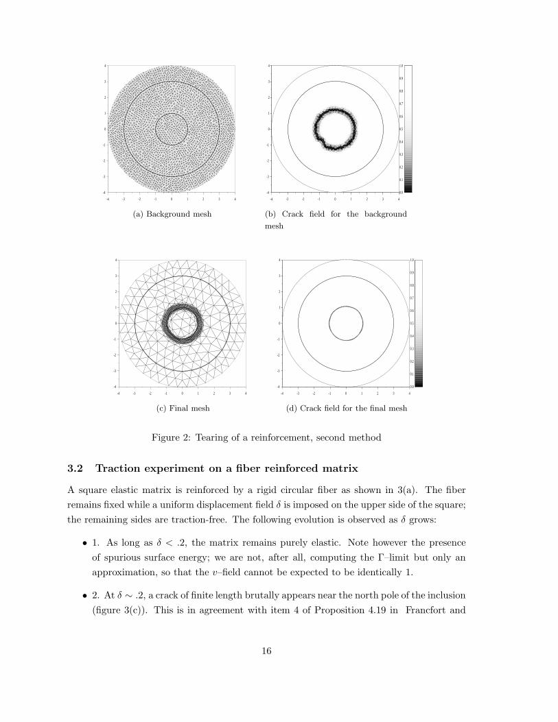
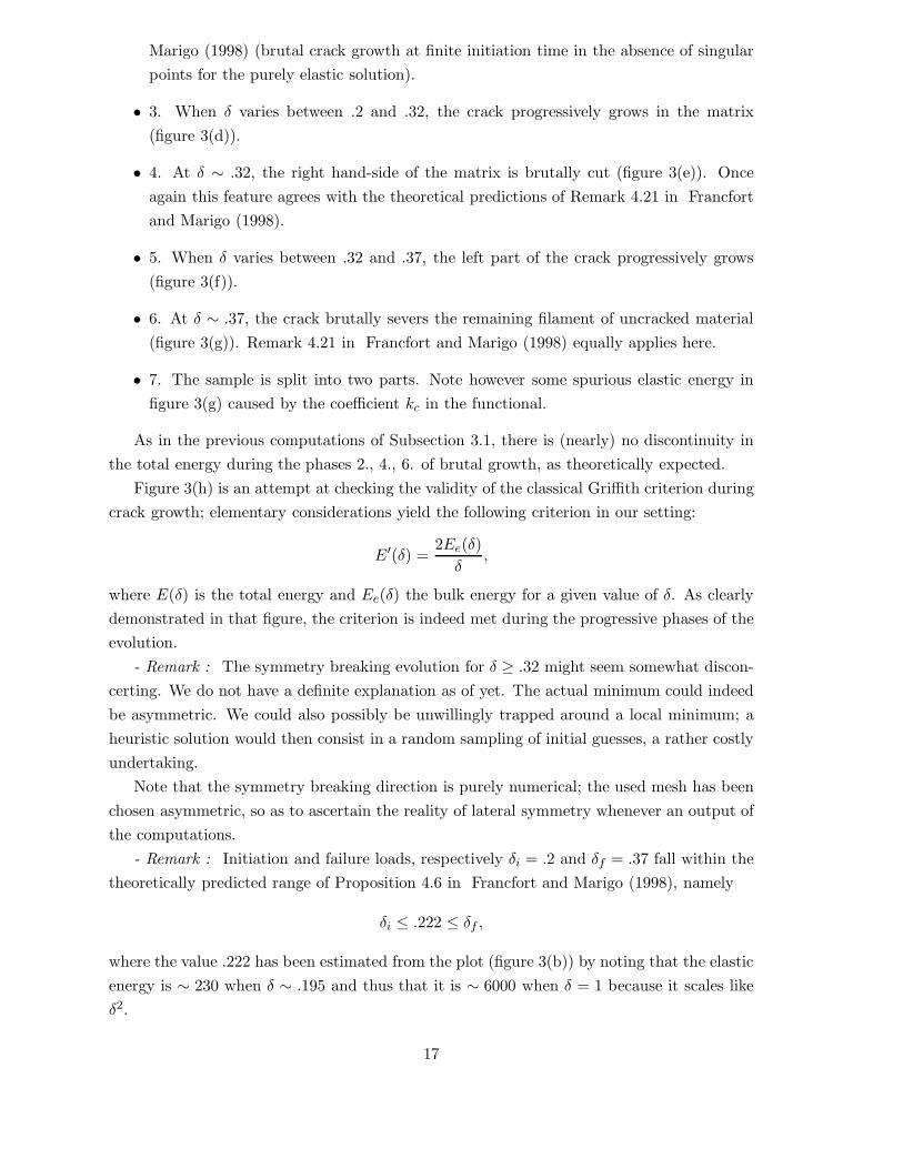
of figure 2, the first mesh (2(a)) is made of 2615 nodes while the last one (2(c)) is made of

only 1005).

13

2.4 Remarks on the plane elasticity case

The study of the plane elasticity problem is still in its infancy. The equivalence between

strong and weak formulation is not established at this time. Furthermore non-interpenetration

of the crack lips should be imposed. The numerical adaptation of the algorithm to a linear

isotropic elasticity problem in the absence of unilateral conditions is similar to that of the

antiplane case. The regularized functional that has to be minimized is

∫

Ω\N(v2 + kc)W (e(u)) dx +

∫

Ω\N(c|∇v|2 +

(1 − v)2

4c) dx, (10)

where W (ξ) = 12tr(ξ)2 + 2e(ξ).e(ξ) (recall that we have chosen to set all constants at 1).

This is the method that has been used for the computations shown in figures 3 and 4. The

result are satisfactory, but can sometimes give results that are not physically admissible (see

for example figure 4(f)). Implementing unilateral conditions is however an open problem as

of yet for want of the proper regularized functional in place of (10).

3 Numerical experiments

In this section three numerical experiments are described and compared with theoretical

predictions, when available. Let us emphasize once again that we do not try and compare our

results with those of true experiments —this will be the object of a forthcoming collaborative

investigation with experimentalists—, but rather strive to test the validity of the presented

computations against the theoretical background developed in Francfort and Marigo (1998).

The color-coded figures presented below represent the v-field for both methods. The crack

site is included within the set of points where that field is near zero (color-coded black in

the figures).

3.1 Tearing of a reinforcement

The tearing of a three-dimensional cylinder of length L can be solved in a closed form

as demonstrated in Francfort and Marigo (1998). A cylinder with annular cross section

of respective inner and outer radii 1 and 3 is considered (see figure 1(a)). It is glued on

its inner surface to a rigid shaft which is submitted to an increasing coaxial displacement

field δ while its outer surface is clamped. Furthermore, the in–section components of the

displacement field, as well as the normal component of the normal stress, are zero at both ends

(u1 = u2 = σ33 = 0, x3 = 0, L).. The analytical result predicts —within our formulation—

the existence of a critical displacement δc =√

2 log 3 ∼ 1.48 such that if δ is less than δc, then

no cracks will appear and the solution is that of the elastic problem, while if δ ≥ δc, a crack

will appear over the entire inner boundary of the material with a surface energy equal to 2π.

The computations presented in figure 1 are obtained with the first method. The parameters

are h = 10−3, c = 10−1, kc = 10−4. In figure 1(b), we plot the bulk energy, surface energy

and total energy versus the load δ. The computed critical load is underestimated but the

14

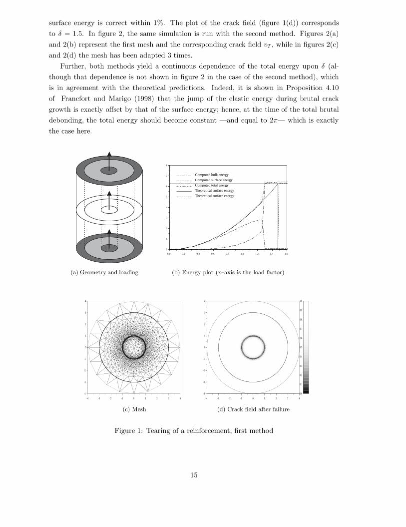
surface energy is correct within 1%. The plot of the crack field (figure 1(d)) corresponds

to δ = 1.5. In figure 2, the same simulation is run with the second method. Figures 2(a)

and 2(b) represent the first mesh and the corresponding crack field vT , while in figures 2(c)

and 2(d) the mesh has been adapted 3 times.

Further, both methods yield a continuous dependence of the total energy upon δ (al-

though that dependence is not shown in figure 2 in the case of the second method), which

is in agreement with the theoretical predictions. Indeed, it is shown in Proposition 4.10

of Francfort and Marigo (1998) that the jump of the elastic energy during brutal crack

growth is exactly offset by that of the surface energy; hence, at the time of the total brutal

debonding, the total energy should become constant —and equal to 2π— which is exactly

the case here.

(a) Geometry and loading

0.0 0.2 0.4 0.6 0.8 1.0 1.2 1.4 1.6

0

1

2

3

4

5

6

7

8

Computed bulk energy

Computed surface energy

Computed total energy

Theoretical surface energy

Theoretical surface energy

(b) Energy plot (x–axis is the load factor)

-4 -3 -2 -1 0 1 2 3 4

-4

-3

-2

-1

0

1

2

3

4

(c) Mesh

-4 -3 -2 -1 0 1 2 3 4

-4

-3

-2

-1

0

1

2

3

4

0.0

0.1

0.2

0.3

0.4

0.5

0.6

0.7

0.8

0.9

1.0

(d) Crack field after failure

Figure 1: Tearing of a reinforcement, first method

15

-4 -3 -2 -1 0 1 2 3 4

-4

-3

-2

-1

0

1

2

3

4

(a) Background mesh

-4 -3 -2 -1 0 1 2 3 4

-4

-3

-2

-1

0

1

2

3

4

0.0

0.1

0.2

0.3

0.4

0.5

0.6

0.7

0.8

0.9

1.0

(b) Crack field for the background

mesh

-4 -3 -2 -1 0 1 2 3 4

-4

-3

-2

-1

0

1

2

3

4

(c) Final mesh

-4 -3 -2 -1 0 1 2 3 4

-4

-3

-2

-1

0

1

2

3

4

0.0

0.1

0.2

0.3

0.4

0.5

0.6

0.7

0.8

0.9

1.0

(d) Crack field for the final mesh

Figure 2: Tearing of a reinforcement, second method

3.2 Traction experiment on a fiber reinforced matrix

A square elastic matrix is reinforced by a rigid circular fiber as shown in 3(a). The fiber

remains fixed while a uniform displacement field δ is imposed on the upper side of the square;

the remaining sides are traction-free. The following evolution is observed as δ grows:

• 1. As long as δ < .2, the matrix remains purely elastic. Note however the presence

of spurious surface energy; we are not, after all, computing the Γ–limit but only an

approximation, so that the v–field cannot be expected to be identically 1.

• 2. At δ ∼ .2, a crack of finite length brutally appears near the north pole of the inclusion

(figure 3(c)). This is in agreement with item 4 of Proposition 4.19 in Francfort and

16

Marigo (1998) (brutal crack growth at finite initiation time in the absence of singular

points for the purely elastic solution).

• 3. When δ varies between .2 and .32, the crack progressively grows in the matrix

(figure 3(d)).

• 4. At δ ∼ .32, the right hand-side of the matrix is brutally cut (figure 3(e)). Once

again this feature agrees with the theoretical predictions of Remark 4.21 in Francfort

and Marigo (1998).

• 5. When δ varies between .32 and .37, the left part of the crack progressively grows

(figure 3(f)).

• 6. At δ ∼ .37, the crack brutally severs the remaining filament of uncracked material

(figure 3(g)). Remark 4.21 in Francfort and Marigo (1998) equally applies here.

• 7. The sample is split into two parts. Note however some spurious elastic energy in

figure 3(g) caused by the coefficient kc in the functional.

As in the previous computations of Subsection 3.1, there is (nearly) no discontinuity in

the total energy during the phases 2., 4., 6. of brutal growth, as theoretically expected.

Figure 3(h) is an attempt at checking the validity of the classical Griffith criterion during

crack growth; elementary considerations yield the following criterion in our setting:

E′(δ) =2Ee(δ)

δ,

where E(δ) is the total energy and Ee(δ) the bulk energy for a given value of δ. As clearly

demonstrated in that figure, the criterion is indeed met during the progressive phases of the

evolution.

- Remark : The symmetry breaking evolution for δ ≥ .32 might seem somewhat discon-

certing. We do not have a definite explanation as of yet. The actual minimum could indeed

be asymmetric. We could also possibly be unwillingly trapped around a local minimum; a

heuristic solution would then consist in a random sampling of initial guesses, a rather costly

undertaking.

Note that the symmetry breaking direction is purely numerical; the used mesh has been

chosen asymmetric, so as to ascertain the reality of lateral symmetry whenever an output of

the computations.

- Remark : Initiation and failure loads, respectively δi = .2 and δf = .37 fall within the

theoretically predicted range of Proposition 4.6 in Francfort and Marigo (1998), namely

δi ≤ .222 ≤ δf ,

where the value .222 has been estimated from the plot (figure 3(b)) by noting that the elastic

energy is ∼ 230 when δ ∼ .195 and thus that it is ∼ 6000 when δ = 1 because it scales like

δ2.

17

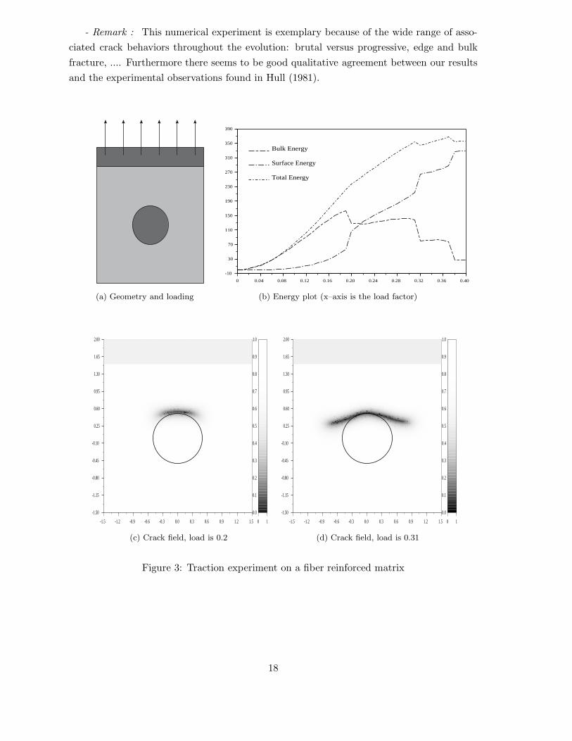
- Remark : This numerical experiment is exemplary because of the wide range of asso-

ciated crack behaviors throughout the evolution: brutal versus progressive, edge and bulk

fracture, .... Furthermore there seems to be good qualitative agreement between our results

and the experimental observations found in Hull (1981).

(a) Geometry and loading

0 0.04 0.08 0.12 0.16 0.20 0.24 0.28 0.32 0.36 0.40

-10

30

70

110

150

190

230

270

310

350

390

Bulk Energy

Surface Energy

Total Energy

(b) Energy plot (x–axis is the load factor)

-1.5 -1.2 -0.9 -0.6 -0.3 0.0 0.3 0.6 0.9 1.2 1.5

-1.50

-1.15

-0.80

-0.45

-0.10

0.25

0.60

0.95

1.30

1.65

2.00

0 1

0.0

0.1

0.2

0.3

0.4

0.5

0.6

0.7

0.8

0.9

1.0

(c) Crack field, load is 0.2

-1.5 -1.2 -0.9 -0.6 -0.3 0.0 0.3 0.6 0.9 1.2 1.5

-1.50

-1.15

-0.80

-0.45

-0.10

0.25

0.60

0.95

1.30

1.65

2.00

0 1

0.0

0.1

0.2

0.3

0.4

0.5

0.6

0.7

0.8

0.9

1.0

(d) Crack field, load is 0.31

Figure 3: Traction experiment on a fiber reinforced matrix

18

-1.5 -1.2 -0.9 -0.6 -0.3 0.0 0.3 0.6 0.9 1.2 1.5

-1.50

-1.15

-0.80

-0.45

-0.10

0.25

0.60

0.95

1.30

1.65

2.00

0 1

0.0

0.1

0.2

0.3

0.4

0.5

0.6

0.7

0.8

0.9

1.0

(e) Crack field, load is 0.32

-1.5 -1.2 -0.9 -0.6 -0.3 0.0 0.3 0.6 0.9 1.2 1.5

-1.50

-1.15

-0.80

-0.45

-0.10

0.25

0.60

0.95

1.30

1.65

2.00

0 1

0.0

0.1

0.2

0.3

0.4

0.5

0.6

0.7

0.8

0.9

1.0

(f) Crack field, load is 0.36

-1.5 -1.2 -0.9 -0.6 -0.3 0.0 0.3 0.6 0.9 1.2 1.5

-1.50

-1.15

-0.80

-0.45

-0.10

0.25

0.60

0.95

1.30

1.65

2.00

0 1

0.0

0.1

0.2

0.3

0.4

0.5

0.6

0.7

0.8

0.9

1.0

(g) Crack field, load is 0.37

+

0.00 0.05 0.10 0.15 0.20 0.25 0.30 0.35 0.40

-1.5

-1.0

-0.5

0.0

0.5

1.0

1.5

0.00 0.05 0.10 0.15 0.20 0.25 0.30 0.35 0.40

-1.5

-1.0

-0.5

0.0

0.5

1.0

1.5

Ο

ΟΟ Ο Ο Ο Ο Ο Ο Ο Ο Ο Ο Ο Ο Ο Ο Ο

ΟΟ Ο Ο

Ο Ο Ο ΟΟ Ο Ο Ο

Ο

Ο Ο ΟΟ Ο

Ο

Ο

(h) Check of Griffith criterion

Figure 3: Traction experiment on a fiber reinforced matrix

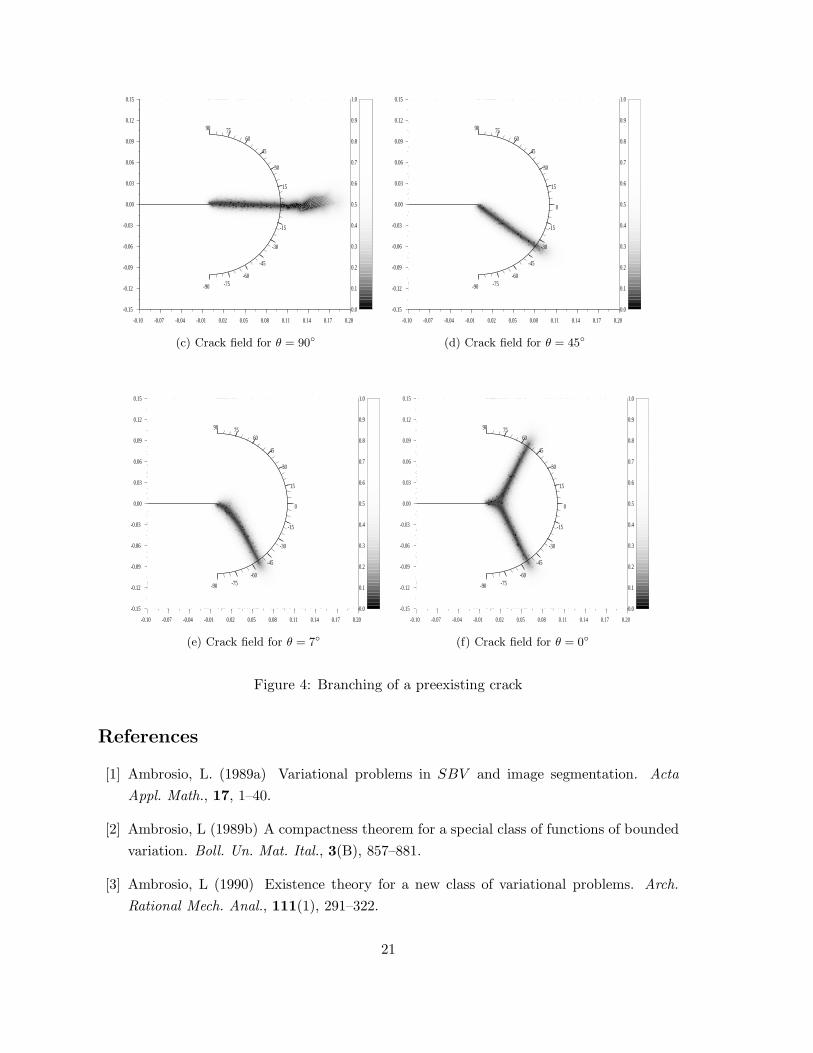
3.3 Crack branching

The branching of a crack is one of the conundrums of brittle fracture. The classical Griffith

theory is inadequate and additional criteria have to be introduced (see e.g. Amestoy (1987),

Amestoy and Leblond (1989), Leblond (1989) and Leguillon (1993)).

19

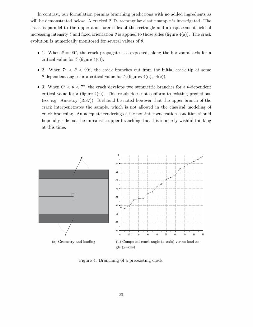
In contrast, our formulation permits branching predictions with no added ingredients as

will be demonstrated below. A cracked 2–D. rectangular elastic sample is investigated. The

crack is parallel to the upper and lower sides of the rectangle and a displacement field of

increasing intensity δ and fixed orientation θ is applied to those sides (figure 4(a)). The crack

evolution is numerically monitored for several values of θ.

• 1. When θ = 90, the crack propagates, as expected, along the horizontal axis for a

critical value for δ (figure 4(c)).

• 2. When 7 < θ < 90, the crack branches out from the initial crack tip at some

θ-dependent angle for a critical value for δ (figures 4(d), 4(e)).

• 3. When 0 < θ < 7, the crack develops two symmetric branches for a θ-dependent

critical value for δ (figure 4(f)). This result does not conform to existing predictions

(see e.g. Amestoy (1987)). It should be noted however that the upper branch of the

crack interpenetrates the sample, which is not allowed in the classical modeling of

crack branching. An adequate rendering of the non-interpenetration condition should

hopefully rule out the unrealistic upper branching, but this is merely wishful thinking

at this time.

(a) Geometry and loading

0 10 20 30 40 50 60 70 80 90

-90

-80

-70

-60

-50

-40

-30

-20

-10

0

0 10 20 30 40 50 60 70 80 90

-90

-80

-70

-60

-50

-40

-30

-20

-10

0

Ο Ο ΟΟ Ο

Ο Ο Ο

ΟΟ

ΟΟ

ΟΟ

Ο

ΟΟ

ΟΟ

ΟΟ

(b) Computed crack angle (x–axis) versus load an-

gle (y–axis)

Figure 4: Branching of a preexisting crack

20

-0.10 -0.07 -0.04 -0.01 0.02 0.05 0.08 0.11 0.14 0.17 0.20

-0.15

-0.12

-0.09

-0.06

-0.03

0.00

0.03

0.06

0.09

0.12

0.15

-90 -75 -60

-45

-30

-15

0

15

30

45

60 75 90

0.0

0.1

0.2

0.3

0.4

0.5

0.6

0.7

0.8

0.9

1.0

(c) Crack field for θ = 90

-0.10 -0.07 -0.04 -0.01 0.02 0.05 0.08 0.11 0.14 0.17 0.20

-0.15

-0.12

-0.09

-0.06

-0.03

0.00

0.03

0.06

0.09

0.12

0.15

-90 -75 -60

-45

-30

-15

0

15

30

45

60 75 90

0.0

0.1

0.2

0.3

0.4

0.5

0.6

0.7

0.8

0.9

1.0

(d) Crack field for θ = 45

-0.10 -0.07 -0.04 -0.01 0.02 0.05 0.08 0.11 0.14 0.17 0.20

-0.15

-0.12

-0.09

-0.06

-0.03

0.00

0.03

0.06

0.09

0.12

0.15

-90 -75 -60

-45

-30

-15

0

15

30

45

60 75 90

0.0

0.1

0.2

0.3

0.4

0.5

0.6

0.7

0.8

0.9

1.0

(e) Crack field for θ = 7

-0.10 -0.07 -0.04 -0.01 0.02 0.05 0.08 0.11 0.14 0.17 0.20

-0.15

-0.12

-0.09

-0.06

-0.03

0.00

0.03

0.06

0.09

0.12

0.15

-90 -75 -60

-45

-30

-15

0

15

30

45

60 75 90

0.0

0.1

0.2

0.3

0.4

0.5

0.6

0.7

0.8

0.9

1.0

(f) Crack field for θ = 0

Figure 4: Branching of a preexisting crack

References

[1] Ambrosio, L. (1989a) Variational problems in SBV and image segmentation. Acta

Appl. Math., 17, 1–40.

[2] Ambrosio, L (1989b) A compactness theorem for a special class of functions of bounded

variation. Boll. Un. Mat. Ital., 3(B), 857–881.

[3] Ambrosio, L (1990) Existence theory for a new class of variational problems. Arch.

Rational Mech. Anal., 111(1), 291–322.

21

[4] Ambrosio, L. and Tortorelli, V.M. (1990) Approximation of functionals depending on

jumps by elliptic functionals via Γ-convergence. Comm. Pure Appl. Math., XLIII,

999–1036.

[5] Ambrosio, L. and Tortorelli, V.M. (1992) On the approximation of free discontinuity

problems. Boll. Un. Mat. Ital. ,7, (6B), 105–123.

[6] Amestoy, M. (1987) Propagations de fissures en elasticite plane. These d’Etat, Paris.

[7] Amestoy, M. and Leblond, J.-B. (1989) Crack path in plane situation -II, detailed form

of the expansion of the stress intensity factors. In. J. Solids Structures, 29(4), 465–501.

[8] Bellettini, G. and Coscia, A.(1994) Discrete approximation of a free discontinuity prob-

lem. Numer. Funct. Anal. Optim, 15, 105–123.

[9] Borouchaki, H. and Laug, P. (1996) Maillage de courbes gouverne par une carte de

metriques. Technical Report RR-2818, INRIA.

[10] Bourdin, B. (1998a) Image segmentation with a finite element method. RAIRO Model.

Math. Anal. Numer., (to appear).

[11] Bourdin, B. (1998b) Une formulation variationnelle en mecanique de la rupture, theorie

et mise en œuvre numerique. These de Doctorat, Universite Paris Nord.

[12] Bourdin, B. and Chambolle, A. (to appear) Implementation of an adaptive finite element

approximation of the Mumford-Shah functional.

[13] Carriero, M. and Leaci, A. (1990) Existence theorem for a Dirichlet problem with free

discontinuity set. Nonlinear Anal., Th. Meth. Appls., 15(7), 661–677.

[14] Chambolle, A. (1998) Finite differences discretizations of the Mumford-Shah functional.

RAIRO Model. Math. Anal. Numer., (to appear).

[15] Chambolle, A. and Dal Maso, G. (1998) Discrete approximation of the Mumford-Shah

functional in dimension two. RAIRO Model. Math. Anal. Numer., (to appear).

[16] De-Giorgi, E., Carriero, M. and Leaci, A. (1989) Existence theorem for a minimum

problem with free discontinuity set. Arch. Rational Mech. Anal., 108, 195–218.

[17] Ekeland, I. and Temam, R. (1976) Convex analysis and variational problems. North-

Holland, Amsterdam.

[18] Finzi-Vita, S. and Perugia, P. (1995) Some numerical experiments on the variational

approach to image segmentation. In Proc. of the Second European Workshop on Image

Processing and Mean Curvature Motion, pp. 233–240, Palma de Mallorca, September

25-27.

22

[19] Francfort, G. and Marigo, J.-J. (1998) Revisiting brittle fracture as an energy mini-

mization problem. J. Mech. Phys. Solids, 46(8), 1319–1342.

[20] Hull, D. (1981) An introduction to composite materials. Cambridge Solid State Science

Series, Cambridge University Press.

[21] Leblond, J.-B. (1989) Crack paths in plane situation - I, general form of the expansion

of the stress intensity factors. In. J. Solids Structures, 25, 1311–1325.

[22] Leguillon, D. (1993) Asymptotic and numerical analysis of a crack branching in non-

isotropic materials. Eur. J. Mech. A/Solids, 12(1), 33–51.

[23] Modica, L. and Mortola, S. (1977) Un esempio di Γ–convergence. Boll. Un. Mat. Ital.,

14-B, 285–299.

[24] Mumford, D. and Shah, J. (1989) Optimal approximation by piecewise smooth functions

and associated variational problems. Comm. Pure Appl. Math., 42, 577–685.

23