Numerical evolutions of Einstein's equations …sfb.aei.mpg.de/Meetings/School04/Talks/Denis1.pdf · Numerical evolutions of Einstein’s equations Denis Pollney Max-Plank-Institut

Numerical evolutions of Einstein’s equations

Denis Pollney

Max-Plank-Institut fur Gravitationsphysik(Albert-Einstein-Institut)

Golm, Germany

SFB School / September 2004

AbstractThis lecture will cover various issues in obtaining numerical solutions of Einstein’s

equations. Formulated as an initial boundary value problem, the field equations become acoupled elliptic-hyperbolic system. Special care needs to be taken in the choice of variables,and form of the evolution system, choice of gauge, and boundary conditions. The lecturewill provide an introduction to these points and discuss current techniques being applied insimulations of black hole spacetimes.

2

Overview

Today: Methods for solving the Einstein equations numerically . . .

• 3+1 formalism

• hyperbolicity, Einstein’s equations, and numerical evolutions

• coordinate conditions

• numerical methods

Friday: Applications . . .

• solving initial data constraints

• quasi-circular orbit parameters for black hole binaries

• tools for analysing spacetime (horizon dynamics, waveform extraction)

• black hole merger simulations

Denis Pollney <[email protected]> Golm / 22 Sep 2004

3

Numerical relativity

• Our goal is to find a solution of a system of non-linear, time-dependent, partialdifferential equations using numerical methods.

Rαβ −1

2gαβR = 8πTαβ

• The equations of the theory are known explicitly; solutions are scarce.

• Numerical solutions involve approximations to the continuum equations, butunlike other approximations:

? don’t impose symmetries or simplifications;? don’t rely on the smallness of relevant physical parameters;? is equipped with error estimates and convergence results.


3



Rαβ −1

2gαβR = 8πTαβ

• The generally covariance of the field equations give rise to a separation intoequations of evolution type, plus constraints.

• A number of different “formulations” have been developed to treat the equations.Differences involve:

? choice of dynamical variables? choice of field equations? choice of coordinate, or classes of coordinate systems? choice of slicing

Mathematical and empirical evidence shows that the choice of formulations canhave significant impact on continuum well-posedness, and thus the ability tocompute a consistent, convergent numerical solution.


3



Rαβ −1

2gαβR = 8πTαβ

Other aspects:

• Don’t expect shocks in the vacuum system.

• There are, however, singularities. These must somehow be avoided in numericalwork.

• Large range of dynamical length scales (from BH horizon to many gravitationalwavelengths).

• Gravitational waves are a small effect – need to be calculated precisely.


4

3+1 decomposition of Einstein equations

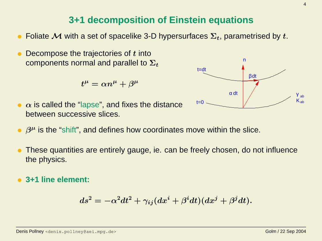
• Foliate M with a set of spacelike 3-D hypersurfaces Σt, parametrised by t.

• Decompose the trajectories of t intocomponents normal and parallel to Σt

tµ = αnµ + βµ

• α is called the “lapse”, and fixes the distancebetween successive slices.

ab

t=0

t=dt

n

βdt

dtαK ab

γ

• βµ is the “shift”, and defines how coordinates move within the slice.

• These quantities are entirely gauge, ie. can be freely chosen, do not influencethe physics.

• 3+1 line element:

ds2 = −α2dt2 + γij(dxi + βidt)(dxj + βjdt).


5


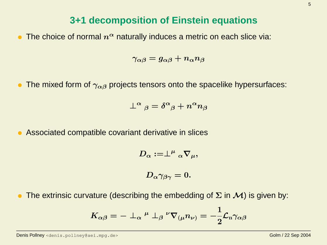
• The choice of normal nα naturally induces a metric on each slice via:

γαβ = gαβ + nαnβ

• The mixed form of γαβ projects tensors onto the spacelike hypersurfaces:

⊥αβ = δαβ + nαnβ

• Associated compatible covariant derivative in slices

Dα :=⊥µα∇µ,

Dαγβγ = 0.

• The extrinsic curvature (describing the embedding of Σ in M) is given by:

Kαβ = − ⊥αµ ⊥β

ν∇(µnν) = −1

2Lnγαβ


6


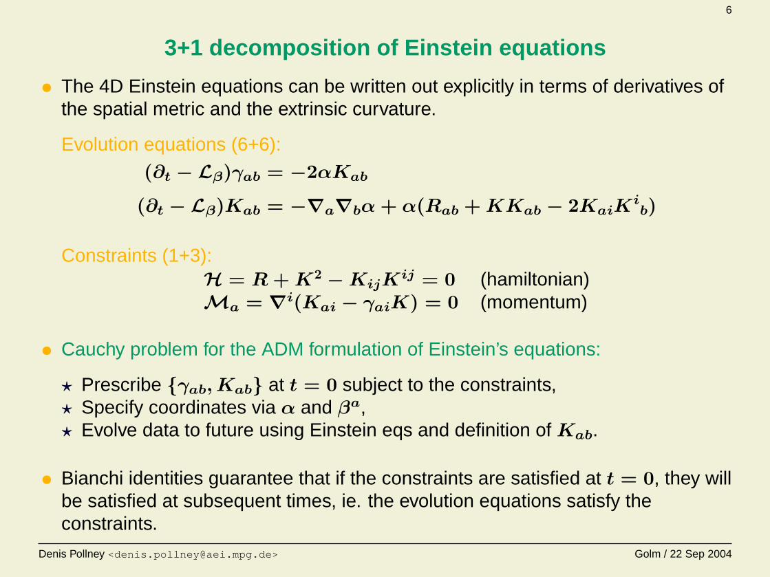
• The 4D Einstein equations can be written out explicitly in terms of derivatives ofthe spatial metric and the extrinsic curvature.

Evolution equations (6+6):

(∂t − Lβ)γab = −2αKab

(∂t − Lβ)Kab = −∇a∇bα+ α(Rab +KKab − 2KaiKib)

Constraints (1+3):H = R+K2 −KijK

ij = 0 (hamiltonian)Ma = ∇i(Kai − γaiK) = 0 (momentum)

• Cauchy problem for the ADM formulation of Einstein’s equations:

? Prescribe {γab,Kab} at t = 0 subject to the constraints,? Specify coordinates via α and βa,? Evolve data to future using Einstein eqs and definition of Kab.

• Bianchi identities guarantee that if the constraints are satisfied at t = 0, they willbe satisfied at subsequent times, ie. the evolution equations satisfy theconstraints.


7

Constraints

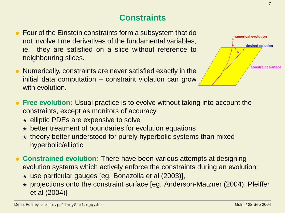
• Four of the Einstein constraints form a subsystem that donot involve time derivatives of the fundamental variables,ie. they are satisfied on a slice without reference toneighbouring slices.

• Numerically, constraints are never satisfied exactly in theinitial data computation – constraint violation can growwith evolution.

numerical evolution

constraint surface

desired solution

• Free evolution: Usual practice is to evolve without taking into account theconstraints, except as monitors of accuracy? elliptic PDEs are expensive to solve? better treatment of boundaries for evolution equations? theory better understood for purely hyperbolic systems than mixed

hyperbolic/elliptic

• Constrained evolution: There have been various attempts at designingevolution systems which actively enforce the constraints during an evolution:? use particular gauges [eg. Bonazolla et al (2003)],? projections onto the constraint surface [eg. Anderson-Matzner (2004), Pfeiffer

et al (2004)]


8

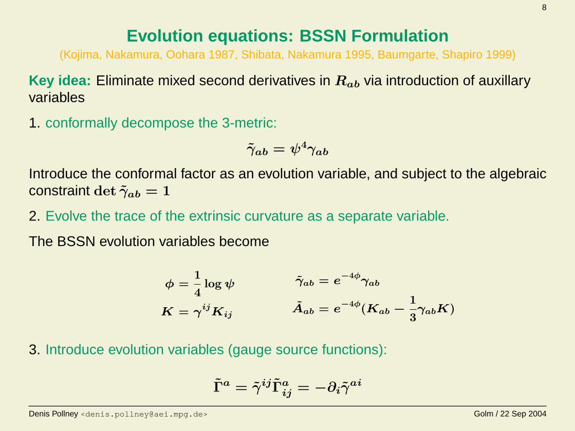
Evolution equations: BSSN Formulation(Kojima, Nakamura, Oohara 1987, Shibata, Nakamura 1995, Baumgarte, Shapiro 1999)

Key idea: Eliminate mixed second derivatives in Rab via introduction of auxillaryvariables

1. conformally decompose the 3-metric:

γab = ψ4γab

Introduce the conformal factor as an evolution variable, and subject to the algebraicconstraint det γab = 1

2. Evolve the trace of the extrinsic curvature as a separate variable.

The BSSN evolution variables become

φ =14

logψ

K = γijKij

γab = e−4φγab

Aab = e−4φ(Kab −

13γabK)

3. Introduce evolution variables (gauge source functions):

Γa = γijΓaij = −∂iγai


9

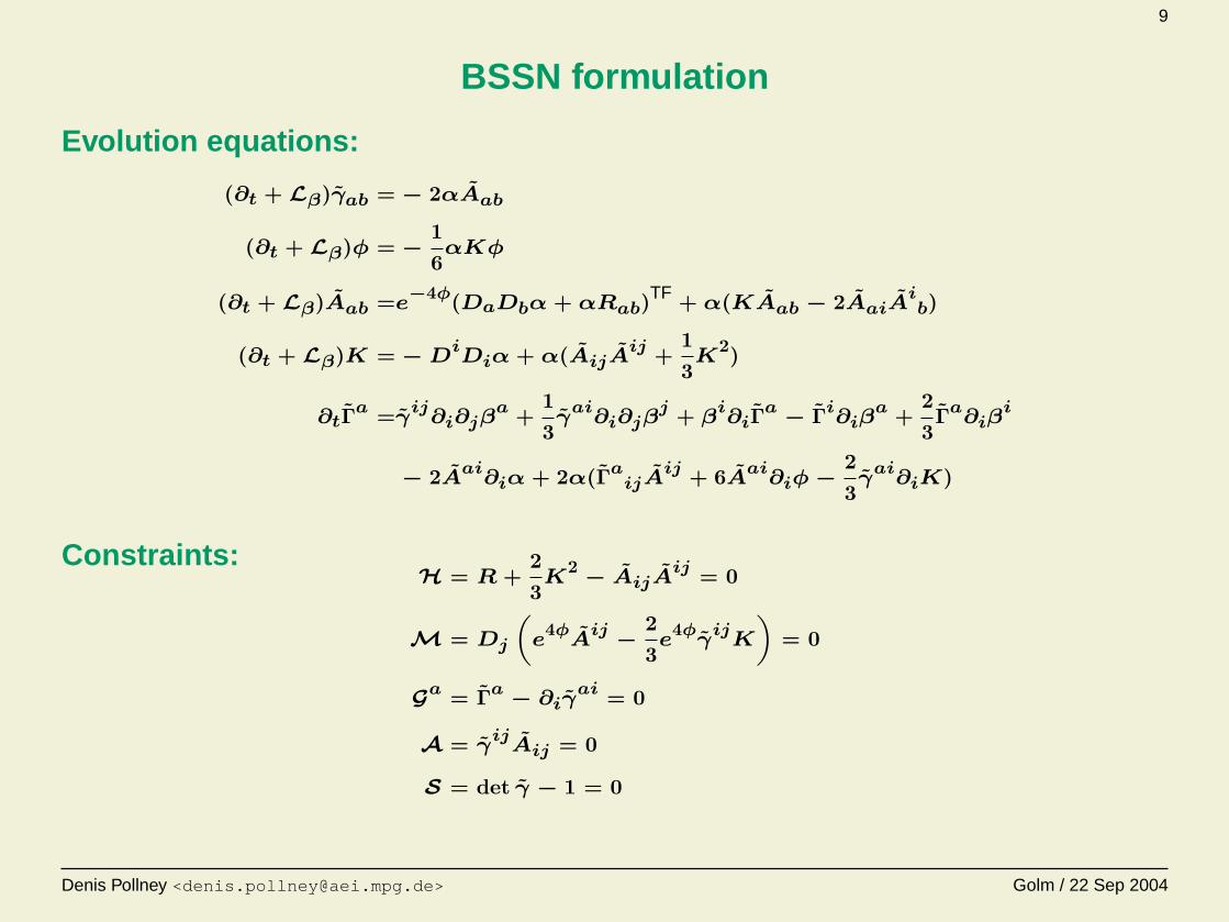
BSSN formulation

Evolution equations:

(∂t + Lβ)γab = − 2αAab

(∂t + Lβ)φ = −16αKφ

(∂t + Lβ)Aab =e−4φ(DaDbα + αRab)TF + α(KAab − 2AaiA

ib)

(∂t + Lβ)K = −DiDiα + α(AijA

ij +13K

2)

∂tΓa =γij∂i∂jβ

a +13γai∂i∂jβ

j + βi∂iΓ

a − Γi∂iβa +

23Γa∂iβ

i

− 2Aai∂iα + 2α(ΓaijAij + 6Aai∂iφ−

23γai∂iK)

Constraints:H = R +

23K

2 − AijAij = 0

M = Dj

„e4φAij −

23e4φγijK

«= 0

Ga = Γa − ∂iγai = 0

A = γijAij = 0

S = det γ − 1 = 0


10

BSSN formulation

0.0 20.0 40.0 60.0 80.0 100.0

t/M

−0.00010

−0.00005

0.00000

0.00005

0.00010

Imψ

4

2D(300x59)

3D(1953x0.5)

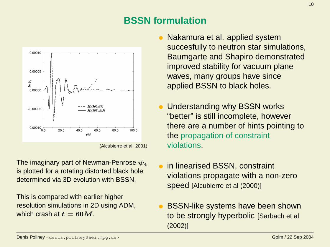
(Alcubierre et al. 2001)

The imaginary part of Newman-Penrose ψ4

is plotted for a rotating distorted black holedetermined via 3D evolution with BSSN.

This is compared with earlier higherresolution simulations in 2D using ADM,which crash at t = 60M .

• Nakamura et al. applied systemsuccesfully to neutron star simulations,Baumgarte and Shapiro demonstratedimproved stability for vacuum planewaves, many groups have sinceapplied BSSN to black holes.

• Understanding why BSSN works“better” is still incomplete, howeverthere are a number of hints pointing tothe propagation of constraintviolations.

• in linearised BSSN, constraintviolations propagate with a non-zerospeed [Alcubierre et al (2000)]

• BSSN-like systems have been shownto be strongly hyperbolic [Sarbach et al(2002)]


11

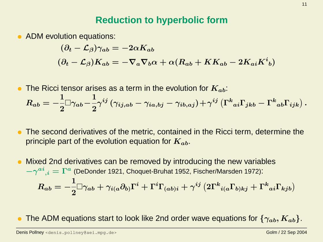
Reduction to hyperbolic form

• ADM evolution equations:

(∂t − Lβ)γab = −2αKab

(∂t − Lβ)Kab = −∇a∇bα+ α(Rab +KKab − 2KaiKib)

• The Ricci tensor arises as a term in the evolution for Kab:

Rab = −1

2�γab−

1

2γij (γij,ab − γia,bj − γib,aj)+γij

(ΓkaiΓjkb − ΓkabΓijk

).

• The second derivatives of the metric, contained in the Ricci term, determine theprinciple part of the evolution equation for Kab.

• Mixed 2nd derivatives can be removed by introducing the new variables−γai,i = Γa (DeDonder 1921, Choquet-Bruhat 1952, Fischer/Marsden 1972):

Rab = −1

2�γab + γi(a∂b)Γi + ΓiΓ(ab)i + γij

(2Γki(aΓb)kj + ΓkaiΓkjb

)

• The ADM equations start to look like 2nd order wave equations for {γab,Kab}.


12

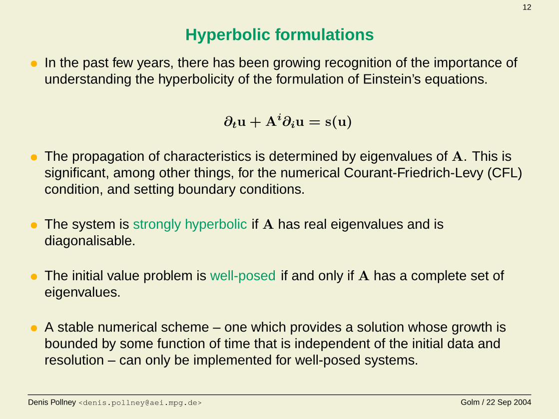
Hyperbolic formulations

• In the past few years, there has been growing recognition of the importance ofunderstanding the hyperbolicity of the formulation of Einstein’s equations.

∂tu + Ai∂iu = s(u)

• The propagation of characteristics is determined by eigenvalues of A. This issignificant, among other things, for the numerical Courant-Friedrich-Levy (CFL)condition, and setting boundary conditions.

• The system is strongly hyperbolic if A has real eigenvalues and isdiagonalisable.

• The initial value problem is well-posed if and only if A has a complete set ofeigenvalues.

• A stable numerical scheme – one which provides a solution whose growth isbounded by some function of time that is independent of the initial data andresolution – can only be implemented for well-posed systems.


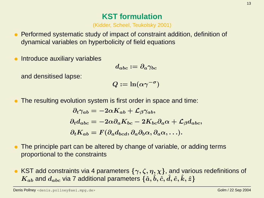
13

KST formulation(Kidder, Scheel, Teukolsky 2001)

• Performed systematic study of impact of constraint addition, definition ofdynamical variables on hyperbolicity of field equations

• Introduce auxiliary variablesdabc := ∂aγbc

and densitised lapse:Q := ln(αγ−σ)

• The resulting evolution system is first order in space and time:

∂tγab = −2αKab + Lβγab,∂tdabc = −2α∂aKbc − 2Kbc∂aα+ Lβdabc,∂tKab = F (∂adbcd, ∂a∂bα, ∂aα, . . .).

• The principle part can be altered by change of variable, or adding termsproportional to the constraints

• KST add constraints via 4 parameters {γ, ζ, η, χ}, and various redefinitions ofKab and dabc via 7 additional parameters {a, b, c, d, e, k, z}


14

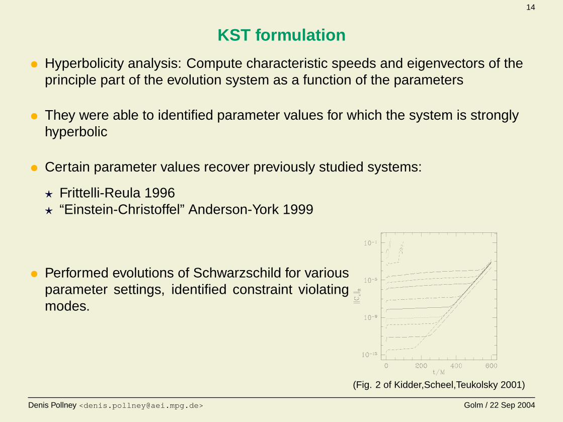
KST formulation

• Hyperbolicity analysis: Compute characteristic speeds and eigenvectors of theprinciple part of the evolution system as a function of the parameters

• They were able to identified parameter values for which the system is stronglyhyperbolic

• Certain parameter values recover previously studied systems:

? Frittelli-Reula 1996? “Einstein-Christoffel” Anderson-York 1999

• Performed evolutions of Schwarzschild for variousparameter settings, identified constraint violatingmodes.

(Fig. 2 of Kidder,Scheel,Teukolsky 2001)


15

Finite-difference schemes for NR

• Time integration is performed via a method of lines technique.

• The PDE system∂tu + Ai∂iu = s(u)

is re-cast into the form of an ODE in time

∂tu = L(u).

• The operator L(u) consists of any suitable spatial discretisation (eg. finitedifference, spectral expansion, finite element).

• Any stable ODE integrator can be used to carry out the time integration(Runge-Kutta, Crank-Nicholson, etc.)


16

Finite-difference schemes for NR

• Symmetric hyperbolic systems can be shown to be well-posed by defining apositive definite energy

E =∫uTHu d3x

over a hypersurface, and showing that it can be bounded as a function of theinitial/boundary data.

• Stable finite-difference schemes can be constructed so that similar energyestimates hold at the discrete level.

• The finite difference analogy to “integration by parts” is “summation by parts”.Introduced to numerical relativity by Calabrese et al. (2003).

• Equations are discretised in space. Scalar product of any two grid functions isdefined and used to construct a semi-discrete energy. The spatial discretisationoperator is defined so that summation by parts holds.

• Stability is ensured by a temporal scheme that preserves the energy estimate.


17

Coordinate conditions

General covariance means that for vacuum relativity, there is no “natural” set ofobservers – no natural coordinate system.

In the 3+1 decomposition, choosing coordinates corresponds to choosing a lapse,α, and shift, βa.

There are a number of features we’d like to see in a good choice of coordinates:

• Cover regions of spacetime of interest

• Simplify equations of motion

? eliminate evolution variables? recast equations into nice form (eg. harmonic coords)

• Simplify the physics (eg. reduce dynamics on the numerical grid)

? minimal distortion (Smarr-York 1978), “symmetry seeking” (Garfinkle-Gundlach 1999)? co-rotating coordinates? known asymptotic states

• Avoid physical singularities

• Computationally efficient

• Compatible with hyperbolicity, well-posedness


18

Coordinate conditions: Examples

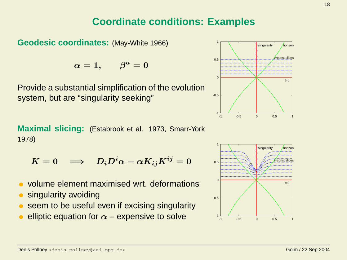
Geodesic coordinates: (May-White 1966)

α = 1, βa = 0

Provide a substantial simplification of the evolutionsystem, but are “singularity seeking”

Maximal slicing: (Estabrook et al. 1973, Smarr-York1978)

K = 0 =⇒ DiDiα− αKijK

ij = 0

• volume element maximised wrt. deformations• singularity avoiding• seem to be useful even if excising singularity• elliptic equation for α – expensive to solve

-1

-0.5

0

0.5

1

-1 -0.5 0 0.5 1

horizon

t=const slices

t=0

singularity

-1

-0.5

0

0.5

1

-1 -0.5 0 0.5 1

horizon

t=const slices

t=0

singularity


19


Generalised harmonic coordinates:

• Coordinate functions are harmonic ∇µ∇µxα = 0

• In terms of lapse and shift:

(∂t − βi∂i)α = −α2K,

(∂t − βi∂i)βa = −α2(γai∂i lnα+ γijΓaij).

• Field equations reduce to non-linear wave equations

• Harmonic slices are only marginally singularity avoiding, and may also develop“coordinate shocks” [Alcubierre 1997]


20


Bona-Mass o slicings

• Introduced by Bona et al. 1995, who considered slicings invariant under spatialcoordinate transformations.

(∂t − βi∂i)α = −α2f(α)K

with f(α) > 0.

? f = 0: Geodesic slicing? f = ∞: Maximal slicing? f = 1: Harmonic slicing? f = 2/α: “1 + log” slicing

• Empirically, “1 + log” slicing has good singularity avoidance properties (similarto maximal) and is computationally inexpensive.

• Widely used in current 3+1 simulations involving black holes.


21


Minimal distortion shift:

• Smarr-York (1978) propose a shift based on minimising changes in theconformal metric during evolution.

• Define:

Θab = 12 ⊥ Ltγab (strain tensor)

Σab = Θab − 13γabΘ

ii (distortion tensor)

• Minimising ΣijΣij under changes of βa leads to:

∇i∇iβa +

1

3∇a∇iβ

i +Raiβi − 2(Kai −

1

3γaiK)∇iα = 0

• A modification of this condition converts it to a hyperbolic “driver” condition –computationally more efficient


22

Conclusions

Stability is the main problem hampering numerical relativity.

Recent experience has shown that successful evolutions require carefulconsideration of

• formulation of Einstein equations

• finite difference techniques

• gauge

In recent years, stability has improved dramatically from improved understanding ofthese issues.

• identification of constraint violating modes

• introduction of sophisticated finite difference techniques

• effective gauges for strong source evolutions

A number of open issues remain, in particular related to the

• coupling between artificial boundary conditions and the interior evolution

• instabilities arising from nonlinear effects, non-principle partsDenis Pollney <[email protected]> Golm / 22 Sep 2004

Documents

Numerical evolutions of Einstein's equations …sfb.aei.mpg.de/Meetings/School04/Talks/Denis1.pdf · Numerical evolutions of Einstein’s equations Denis Pollney Max-Plank-Institut