Metals 2015, 5, 1-xmanuscripts; doi:10.3390/met50x000x

metals ISSN 2075-4701

www.mdpi.com/journal/metals/ Article

Numerical evaluation of temperature field and residual stresses in an API 5L X80 steel welded joint using the finite element method

Jailson A. Da Nóbrega1, Diego D. S. Diniz2, Antonio A. Silva1, Theophilo M. Maciel1, Victor Hugo C. de Albuquerque3 and João Manuel R. S. Tavares4, *

1 Universidade Federal de Campina Grande (UFCG), Campina Grande-PB, Brazil; E-Mails: jailson_engmec@hotmail.com; antonio.almeida@ufcg.edu.br; theophilo.maciel@ufcg.edu.br

2 Universidade Federal Rural do Semi-Árido (UFERSA), Caraúbas-RN, Brazil; E-Mails: diego.diniz@ufersa.edu.br

3 Programa de Pós-Graduação em Informática Aplicada, Universidade de Fortaleza, Fortaleza-CE, 60811-905, Brazil; E-Mail: victor.albuquerque@unifor.br

4 Instituto de Ciência e Inovação em Engenharia Mecânica e Industrial, Departamento de Engenharia Mecânica, Universidade do Porto, 4200-465, Portugal; E-Mail: tavares@fe.up.pt

* Author to whom correspondence should be addressed; E-Mail: tavares@fe.up.pt; Tel.: +351 22 508 1487.

Academic Editor:

Abstract: Metallic materials undergo many metallurgical changes when subjected to welding thermal cycles, and these changes have a considerable influence on the thermo-mechanical properties of welded structures. One method for evaluating the welding thermal cycle variables, while still in the project phase, would be simulation using computational methods. This paper presents an evaluation of the temperature field and residual stresses in a multipass weld of API 5L X80 steel, which is extensively used in oil and gas industry, using the Finite Element Method (FEM). In the simulation, the following complex phenomena were considered: the variation in physical and mechanical properties of the material as a function of the temperature, welding speed and convection and radiation mechanisms. Additionally, in order to characterize a multipass weld using the Gas Tungsten Arc Welding process for the root pass and the Shielded Metal Arc Welding process for the filling passes, the analytical heat source proposed by Goldak & Chakravarti was used. Also we were able to analyze the influence of the mesh refinement in the simulation results. The findings indicated a significant variation of about 50% in the peak

OPEN ACCESS

Metals2015, 5 2

temperature values. Furthermore, changes were observed in terms of the level and profile of the welded joint residual stresses when more than one welding pass was considered.

Keywords: Multipass welding; temperature field; residual stress; finite element method; computer simulation

1. Introduction

The materials, in welded joints, undergo many metallurgical changes due to the intense localized heat input, particularly for fusion welding. This heat input takes place in a nonlinear and transient manner, with the main heat input near the heat source and a lesser heat input coming from the center of the welding zone. Thus, non-uniform elastic and plastic deformations are generated promoting high residual stresses in the welded joint [1]. The level and profile of residual stresses exert a considerable influence on the welded joint properties and their control can avoid possible structural failures [2]. Thus, the influence of the residual stresses on the crack growth of welded joints is the focus of many studies concerning engineering applications [3, 4], as well as in the optimization of turbine flanges [5] and in the petroleum industries [6], just to name some examples. Therefore, various destructive and non-destructive techniques have been used to evaluate the residual stresses in welded joints. Currently, one of the non-destructive methods is computational analysis based on analytical methods.

The Finite Element Method (FEM) has been used to evaluate the weld thermal cycle, by various authors such as Cho et al. [7] and Robertsson & Svedman [8] who used the commercial software ANSYS® and SIMULIA ABAQUS®, respectively. These authors found excellent results in the thermal and structural analyses compared to the experimental ones obtained by thermocouples inserted in the welded joint for temperature measurements and X-ray diffraction to assess the residual stresses.

Methods of numerical analysis can provide benefits to many areas of engineering, from the development of new products to maintenance services. In manufacturing, the welding parameters can be pre-established to minimize distortions and residual stresses caused by plastic deformation and thermal expansion, without the need to carry out costly laboratory experiments. In some cases, control models can be developed from the inversion of computational models in order to perform real-time corrections in the welding process and prevent variations that can produce weak points in components [abariki, 10, 11].

The purpose of this study was to simulate and evaluate the temperature field and residual stresses in an API 5L X80 steel welded joint using the GTAW (Gas Tungsten Arc Welding) process and SMAW (Shielded Metal Arc Welding) process, through the use of the commercial software ABAQUS®, which is based on FEM. This work studies the evolution of the thermal cycles and residual stresses by employing a single welding process or a combination of multiple welding passes, thereby making the computational simulation more realistic.

2. Mathematical model

2.1. Thermal Modeling

Metals2015, 5 3

In the electric arc welding process, an electrical source generates a voltage U between the electrode and the base metal, inducing the formation of an electric arc traversed by a current I. In this process, energy losses occur through several factors, among them, the convection and radiation in the electric arc can be mentioned. Consequently, only a portion of this energy is used to melt the material, and therefore it is necessary to add a variable called power efficiency (η). Hence, the effective weld heat input can be given as:

𝑄 = 𝜂.𝑈. 𝐼. (1)

In this thermal model, the thermal gradient can be assessed by establishing the related energy balance:

𝜌 𝑇 𝑐 𝑇 !!!!= 𝑄 + !

!"𝐾! 𝑇

!"!"

+ !!"

𝐾! 𝑇!"!"

+ !!"

𝐾! 𝑇!"!"

, (2)

where ρ is the material density, c is the specific heat, Q is the heat input (Eq. 1), Kx, Ky, Kz are the thermal conductivity coefficients in each direction, T is the temperature and t the time. The associated heat flow is not linear, and the thermophysical properties of the material are highly dependent on the temperature.

The heat loss by convection qc and radiation qr can be calculated using the following equations:

𝑞! = ℎ!(𝑇 − 𝑇!), and (3)

𝑞! = 𝜀𝜎(𝑇! − 𝑇!!), (4)

where hf is the convective coefficient, T∞ is the ambient temperature, σ is the Stefan-Boltzmann constant and ε the emissivity of the body surface.

A phase change occurs during the process and this generates a latent heat, which can be expressed as a function of the enthalpy (H) as:

𝐻 = 𝜌𝑐𝑑𝑇. (5)

For computational analysis by FEM, an essential issue in the simulation is the modeling of the heat source. Goldak & Chakravarti [12] proposed an analytical solution for modeling the distributed heat source associated to the arc welding which is commonly used in this type of analysis. Therefore, the temperature field can be determined, computationally, based on a 3D finite Gaussian on a double ellipsoid, as shown in Figure 1. This heat source is analytically defined by the equations [13]:

𝑞! 𝑥,𝑦, 𝑧 = 𝑓!!"#

!!!"# !6 3𝑒

(!!!!

!!! )𝑒(

!!!!

!!)𝑒(

!!!!

!!), and (6)

𝑞! 𝑥,𝑦, 𝑧 = 𝑓!!"#

!!!"# !6 3𝑒

(!!!!

!!!)𝑒(

!!!!

!!)𝑒(

!!!!

!!), (7)

where qf and qr are the volumetric energy distributions before and after the torch [W/m3], and ff and fr are the fractional factors of the distributions of the accumulated heat before and after the torch [14] (Figure 1). Additionally, U, I, η are parameters directly linked to the welding procedures, while b and d are the geometric parameters of the heat source and can be determined by metallographic examination. The other parameters af, ar, ff and fr are obtained through the parameters b and d; furthermore, the sum of ff and fr is equal to 2 [12]. In the absence of better data, the distance (af) from the triad reference

Metals2015, 5 4

point to the front of the heat source is defined as being equal to half the width of the weld and the distance (ar) from the reference point to behind the heat source is defined as being equal to twice the width; this procedure has led to good approximations [13].

Figure 1. 3D Volumetric Gaussian on a double ellipsoidal of radius a, b and d.

Due to the tighter specifications and control of modern steels, thermal analysis is of great importance to estimate the correct preheating temperature value for reliable welding. For example, Cooper et al. [15] compared four methods for calculating the preheating temperature of structural steels, including the API 5L grade X80. The four methods used were: a) the British Standard Institution method (BS 5135) based on the CE value (IIW), b) the American Welding Society method (AWS D1.1) that calculates the temperature of preheating through Pcm, c) the TCE method (Total Carbon Equivalent) which calculates the temperature of preheating as a function of the CE, material thickness, diffusible hydrogen in the weld metal and the heat input, and d) the CEN method.

In this work, the preheating temperature value was based on the study of Cooper et al. [15] and the experimental work conducted by Araújo [16]. The preheating temperature value was defined as being equal to 100 °C corresponding to the BS method, which is the most conservative method of those considered by Cooper et al.. The interpass temperature value was 150 °C following the N-133J standard [17]. 2.2. Residual Stresses Model

The movement of the welding electric arc generates a non-linear thermal gradient and the thermal and mechanical changes arising from the heat source promote thermal stresses and distortions. Therefore, based on the thermal gradients given by Equation 2, the residual stresses based on the deformations caused by the gradients can be determined according to:

𝜎! = 𝛿! 𝜆𝜀!! + 2𝜇𝜀! − 𝛿! (3𝜆 + 2𝜇)𝛼𝑇, (8)

where λ and µ are the Lame constants, which represent the components of the material deformation due to the temperature and are related to the material elasticity modulus E and Poisson's ratio v. The 𝜀! variable is linked to the deformation and displacement according to:

𝜀! = !!

!!!!!!

+ !!!!!!

. (9)

The model used for determining the residual stresses was elastoplastic with isotropic hardening and the correspondent values were obtained from the strains generated during the welding process.

The strains were considered to have elastic, plastic and thermal natures; so, the total strain was determined as:

Metals2015, 5 5

𝜀!" = 𝜀!"! + 𝜀!"! + 𝜀!"!!, (10)

where εij is the total deformation, εije the elastic deformation, εijp the plastic deformation and εijth the thermal deformation.

Based on the Hooke's law, the elastic deformation can be written as:

𝜀 !"! = 𝜎!"! .𝐸(𝑇)!!. (11)

On the other hand, the deformation due to the thermal effect is given as:

𝜀 !"!! = 𝛼!"( 𝑇 − 𝑇!

), (12)

where αij is the thermal coefficient of linear expansion and T∞ is the reference temperature. This thermal deformation depends on the phase of the material.

The theory of plasticity describes the elastic-plastic response of materials through mathematical relationships based on some restrictive assumptions. Among these assumptions, it can be assumed that plastic deformation is the result of a history of tensions that occurred instantaneously, i.e., independently of time [18].

Using the model of the flow rule, which establishes the direction of plasticity for metal materials under conditions of small displacements, the plastic potential function g is equal to the flow area capability f. This relation is known as the associated flow rule, and the direction of plasticity is considered to be normal to the flow surface. The plastic strain ratio is determined as:

𝑑𝜀 !"!" = 𝑑𝜆

!"!!!"

, (13)

where λ is a positive constant dependent on the properties of the material. For a perfect elastic-plastic material and for the cases in which a Von Mises surface is used as flow area capability criterion, the parameter λ can be described as:

𝜆 =!!!!"!!"!!!

. (14)

Further details can be seen in the works of Akbari & Sattari-Far [9], Syahroni & Hidayat [10], Queresh [13], Depraudeux [19] and Yao Xin et al. [20].

3. Material and Computational Simulation

The computational model was developed in ABAQUS® version 6.12, which is based on FEM. The workpiece was an API 5L X80 steel plate 0.120x0.360x0.017 m3, which is the same as the one used in the experimental work of Araújo [16]. The chemical composition of this steel is shown in Table 1.

Table 1. Chemical composition of the API 5L X80 steel.

Percentage (%) by weight

C Mn Si P S Ni Mo Al Cr V Cu 0.084 1.61 0.23 0.01 0.011 0.17 0.17 0.035 0.135 0.015 0.029

The majority of the published works on numerical simulation of welding processes considers that the material properties are highly dependent on temperature. However, it is very difficult to obtain

Metals2015, 5 6

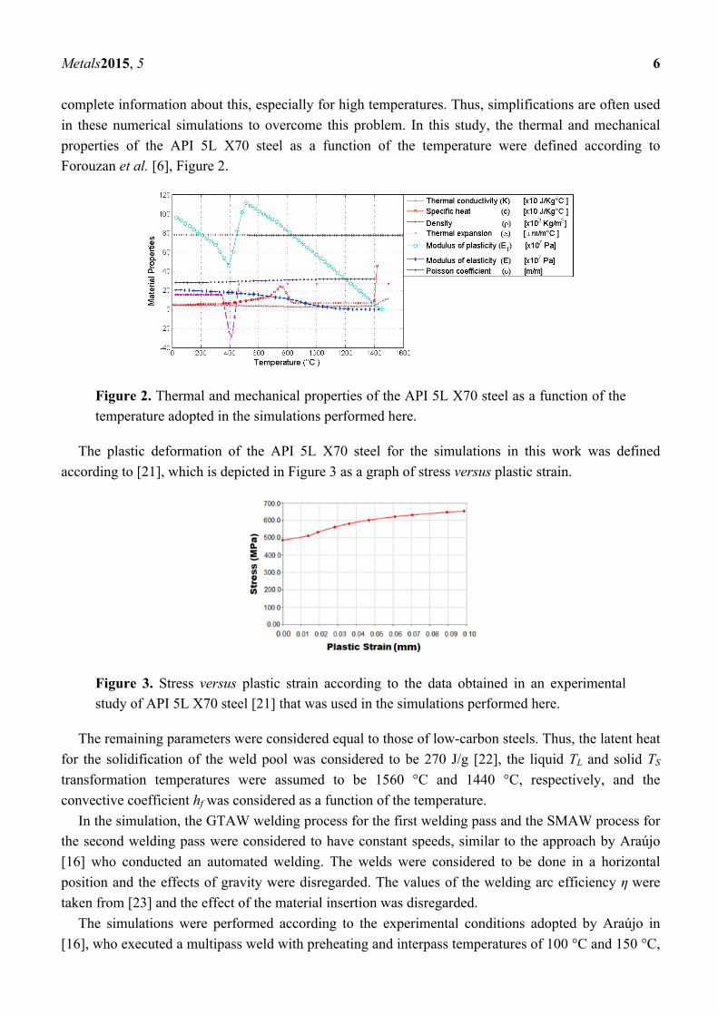
complete information about this, especially for high temperatures. Thus, simplifications are often used in these numerical simulations to overcome this problem. In this study, the thermal and mechanical properties of the API 5L X70 steel as a function of the temperature were defined according to Forouzan et al. [6], Figure 2.

Figure 2. Thermal and mechanical properties of the API 5L X70 steel as a function of the temperature adopted in the simulations performed here.

The plastic deformation of the API 5L X70 steel for the simulations in this work was defined according to [21], which is depicted in Figure 3 as a graph of stress versus plastic strain.

Figure 3. Stress versus plastic strain according to the data obtained in an experimental study of API 5L X70 steel [21] that was used in the simulations performed here.

The remaining parameters were considered equal to those of low-carbon steels. Thus, the latent heat for the solidification of the weld pool was considered to be 270 J/g [22], the liquid TL and solid TS transformation temperatures were assumed to be 1560 °C and 1440 °C, respectively, and the convective coefficient hf was considered as a function of the temperature.

In the simulation, the GTAW welding process for the first welding pass and the SMAW process for the second welding pass were considered to have constant speeds, similar to the approach by Araújo [16] who conducted an automated welding. The welds were considered to be done in a horizontal position and the effects of gravity were disregarded. The values of the welding arc efficiency ƞ were taken from [23] and the effect of the material insertion was disregarded.

The simulations were performed according to the experimental conditions adopted by Araújo in [16], who executed a multipass weld with preheating and interpass temperatures of 100 °C and 150 °C,

Metals2015, 5 7

respectively, according to the N-133J standard [17]. The welding variables and geometric parameters of the welding passes used in the simulations are shown in Table 2.

Table 2.Welding parameters used in the simulations. (1°pass) GTAW (2°pass) SMAW

ε (%) V(m/s) I (A) U (V) Ε (%) V (m/s) I (A) U(V) 65 0.0012 152 12 80 0.0015 69 33

af (m) ar (m) b (m) d (m) af ( m) ar (m) b (m) d (m) 0.00245 0.0098 0.00245 0.00403 0.0043 0.0172 0.0043 0.00376

To represent the required welding conditions, the model of Goldak & Chakravarti [12] was applied

and developed in a DFLUX subroutine in FORTRAN and integrated in ABAQUS®. Figure 4 shows the detailed steps of the computational model used to perform the thermal and

thermo-mechanical simulations.

Figure 4. Detailed sequence of preprocessing, processing and post-processing developed in the thermal and thermo-mechanical simulations.

Metals2015, 5 8

The choice of the mesh used in computer simulations is of fundamental importance as a refined mesh usually leads to results of greater robustness and reliability due to an increase in the number of degrees of freedom. However, the mesh refinement must be carried out carefully, as this also will result in an increased computational cost. In this work, convergence tests were performed on the meshing process. The maximum temperature reached on the weld pool was considered as the reference point for the mesh refinement as was considered by Queresh in [13]; however, the mesh refinement in terms of the thermo-mechanical effects was not considered, due to the associated high computational cost. The response of the refinement process used is shown in Figure 5.

Figure 5. Mesh refinement based on the maximum temperature in the weld pool.

After the convergence tests, the optimized configuration of the mesh refinement led to three main regions, which are depicted in Figures 6 and 7. Each region has a specific number of elements, as shown in Table 3. As aforementioned, for the thermo-mechanical simulation, the mesh refinement was disregarded, since it would increase the computational cost and the simulation time considerably. The elements DC3D8 and C3D8T were used in the thermal and thermo-mechanical simulations, respectively [24].

Table 3. Number of elements of the FEM mesh of each region studied (indicated in Figures 6 and 7).

Model Number of elements Region 1 Region 2 Region 3 Total

Thermal 24,480 41,616 -------- 66,096 Thermo-mechanical 3,640 4,480 5,600 13,720

In the thermal simulation, only half of the plate was considered, since the phenomenon and the conditions used allowed the application of the symmetry theory [25]. In addition, to create a region of higher mesh refinement, the partition (Region 3) at 0.02 m distance from where the heat source passes was defined, due to a higher probability of occurrence of thermal transformations at this location. Such procedure was also adopted in [13, 18, 25].

The thermal boundary conditions for the heat exchanged by radiation and convection were defined in the model for five sides of the plate; the sixth side supported by the table was excluded. This is in

Metals2015, 5 9

accordance with experimental laboratory procedures, and therefore, the hypothesis of zero heat exchange with the table was adopted. The values of these boundary conditions were defined as: ambient temperature of 25 °C, Stefan-Boltzmann constant equal to 5.67x10-8 W.m-2.K-4 and emissivity of 0.77, which were obtained from [26], while the hf value was defined according to [13].

The movement of the heat source is shown in Figure 6. The first welding pass was carried out along the XY plane, with the movement of the heat source along the Y axis. The second welding pass was carried out following the same procedure; however, it was displaced vertically 0.004 m along the Z-axis. The computational thermal evaluation was conducted on the node 0.002 m from the root pass fusion line. The 0.05 m extremities of the plate ends were disregarded, which is in-line with the conditions adopted in a laboratory due to the fixing clips [16].

Figure 6. Movement of the welding heat source for the two welding passes. The second pass was initiated when the temperature at the end of the first pass region dropped to 150 °C.

After the two welding passes, the transverse residual stresses were analyzed in three different positions (beginning, middle and terminal), using the average value for each region, Figure 7. The positions to evaluate these stresses are similar to those followed by Araújo in [16].

Figure 7. Three positions were analyzed in terms of the transverse residual stresses: beginning, middle and terminal; at each position, the average values based on three reference lines 80 mm long and 0.045 mm equidistant from each other were used.

Region 1

Region 2

Region 3

Region 2

Region 1

Metals2015, 5 10

3. Results and Discussion

In order to validate the computational model used in the simulations, the welding of an API 5LX70 steel plate with dimensions of 0.1x0.1x0.019 m3, and the same experimental parameters and conditions used by Laursen et al. [27] were employed here. The authors used a current of 140 A, a voltage of 23V and an automated speed equal to 0.001 m/s to performing the root pass at room temperature (25 °C). After convergence tests, it was found that the model with 30000 elements converges to the maximum temperature results in the monitored region. The same conditions of thermal contours described in [27] were employed here, except for the geometric parameters af, ar, b and d, energy parameters ff and fr, and the weld pool that were obtained from the literature [28, 13]. The virtual thermal cycling was evaluated here in the same region considered in [27], and is shown in Figure 8.

Figure 8: Comparative thermal cycle analysis of the experimental and the numerical method.

The comparative thermal cycle showed a good similarity in terms of the shape of the curves between the experimental and numerical processes (Figure 8); however, the numerical curve had a bandwidth greater than the experimental process. Some assumptions may explain the differences found. The lack of material data and the simplifications adopted may hinder a better approximation between the real and the computational results. According to Heinze et al. [29], the diameter of the thermocouple and its position may influence the comparison between the experimental and computer modeling since the computing node has an accuracy greater than the thermocouple positioned in the welded joint. The computational values of the peak temperature and ∆t8/5 were 1062.30 °C and 7.60 seconds, respectively, while the experimental ones were 1055.55 °C and 6.81 seconds, causing an error inferior to 1% as to the peak temperature and of 11.60% for the ∆t8/5 value.

The results of the thermal analysis obtained from the simulation were consistent and close to other results obtained computationally, and the errors were in agreement with those obtained by Heinze et al. [29], who found errors up to 14%. This close approximation of the peak temperature was due to the Goldak heat source model used [14], which closely portrays the heat source in the experiment and because it also applied accurate values of this heat source; therefore, when the simulated heat source is at the location of where the workpiece is under analysis an error of less than 1% was obtained.

Figures 9 and 10 show the temperature gradients obtained in the simulated welding when the heat source is at the center of the plate. Figure 11 shows the thermal cycles at the beginning, middle and terminal of the welding process for the two welding passes.

Metals2015, 5 11

Figure 9. Temperature gradient obtained when the virtual source of heat is in the middle of the first welding pass.

Figure 10. Temperature gradient obtained when the virtual source of heat is in the middle of the second welding pass.

Figures 9 and 10 show that the maximum temperatures are located close to and just behind the heat source, and that several isotherms with lower temperatures arise from the end of the plate, developing a temperature gradient along the plate, as reported by Kenneth [30]. There was a variation in the maximum temperature between the welding passes: 1655 °C and 1706 °C for the 1st and 2nd passes, respectively. This variation may have occurred due to variations in the welding speed although the welding energy used was constant. This fact was also observed in previous studies, such as the ones by Deng & Kiyoshima [31], Samardžić et al. [32], Zhu & Chao [33] and Nandan et al. [34].

Figure 11. Temperature cycles evaluated at the beginning, middle and end of the welding process at a point located 0.002 m from the heat source.

Metals2015, 5 12

Table 4 indicates the cooling time between the 800 °C and 500 °C thermal cycles of the curves of Figure 11.

Table 4. Cooling time between 800-500 °C (∆t8/5) values at 0.002 m from the fusion line.

∆t8/5

Beginning

(s)

∆t8/5

Middle

(s)

∆t8/5

Terminal

(s)

∆t8/5

Average

(s)

Variation (%)

1°pass 3.71 4.02 3.30 3.68 22.00

2°pass 22.50 26.89 27.30 25.56 21.00

Table 4 shows that there were variations of up to 22% in Δt8/5 when it was assessed at different

points in the region under study (beginning, middle and end of the weld joint). The largest cooling time of 27.30 s is located at the end of the second simulated welding pass.

Figure 12 shows a comparison between the transverse residual stresses computationally obtained at the beginning, middle and end of the weld joint after the simulated welding with one pass and two passes until cooling to the ambient temperature.

(a) (b)

Figure 12. Transverse residual stresses located at the beginning, middle and end, after the first simulated welding pass until cooling to room temperature (a), and after two simulated welding passes until cooling to room temperature (b).

Figure 12a shows a predominance of traction residual stresses in the center region of the welded joint that corresponds to the weld metal, with stresses varying from 240 to -300 MPa, and compressive stress from -120 to -200 MPa in the regions near the fusion line. This behavior was also observed in the work by Stamenković & Vasovic [35], who performed a computer simulation with a virtual welding pass. On the other hand, Figure 12b shows that there was a change in the level of the residual transverse stresses when the second welding pass was applied on the first one. The traction residual stresses tend to be reduced. Therefore on considering a greater number of passes in the simulated

Metals2015, 5 13

welding, there is a tendency for decreased tensions, and the profile of the residual stresses after the fusion line region becomes more alike to the ones observed experimentally by Araújo [16].

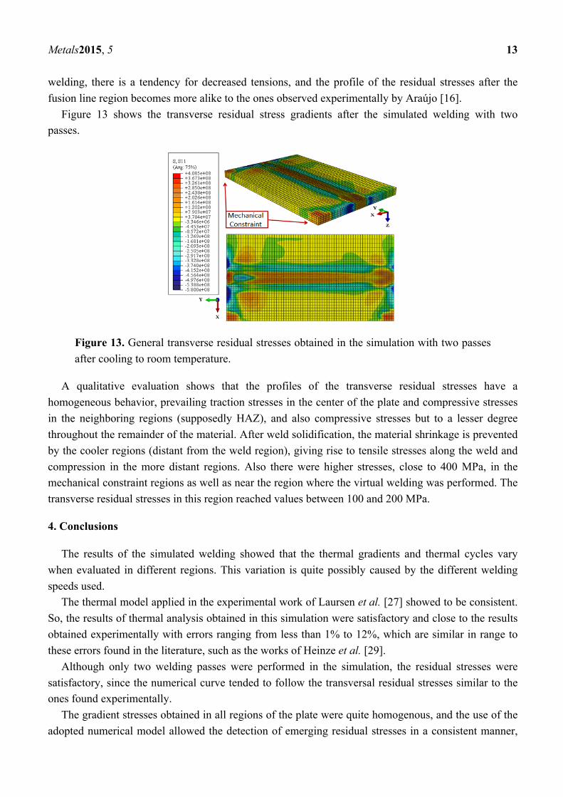
Figure 13 shows the transverse residual stress gradients after the simulated welding with two passes.

Figure 13. General transverse residual stresses obtained in the simulation with two passes after cooling to room temperature.

A qualitative evaluation shows that the profiles of the transverse residual stresses have a homogeneous behavior, prevailing traction stresses in the center of the plate and compressive stresses in the neighboring regions (supposedly HAZ), and also compressive stresses but to a lesser degree throughout the remainder of the material. After weld solidification, the material shrinkage is prevented by the cooler regions (distant from the weld region), giving rise to tensile stresses along the weld and compression in the more distant regions. Also there were higher stresses, close to 400 MPa, in the mechanical constraint regions as well as near the region where the virtual welding was performed. The transverse residual stresses in this region reached values between 100 and 200 MPa.

4. Conclusions

The results of the simulated welding showed that the thermal gradients and thermal cycles vary when evaluated in different regions. This variation is quite possibly caused by the different welding speeds used.

The thermal model applied in the experimental work of Laursen et al. [27] showed to be consistent. So, the results of thermal analysis obtained in this simulation were satisfactory and close to the results obtained experimentally with errors ranging from less than 1% to 12%, which are similar in range to these errors found in the literature, such as the works of Heinze et al. [29].

Although only two welding passes were performed in the simulation, the residual stresses were satisfactory, since the numerical curve tended to follow the transversal residual stresses similar to the ones found experimentally.

The gradient stresses obtained in all regions of the plate were quite homogenous, and the use of the adopted numerical model allowed the detection of emerging residual stresses in a consistent manner,

Metals2015, 5 14

with the highest levels of traction stresses in the central regions of the welded joint and compressive in more distant regions.

Possible future works could be related to the mesh refinement based on the residual stress which can lead to important insights for more competent welding processes although this type of mesh refinement can lead to high computational costs. Also interesting for such a goal would be investigations into the influence of the properties of the temperature-dependent and -independent materials on the simulation results.

Acknowledgments

The authors thank the Academic Unit of Mechanical Engineering and Postgraduate Program in Mechanical Engineering from the Federal University of Campina Grande and the Coordination for the Improvement of Higher Education Personnel (CAPES) in Brazil for the financial support.

Victor Hugo C. de Albuquerque acknowledges the sponsorship from the Brazilian National Council for Research and Development (CNPq) through the grants with references 470501/2013-8 and 301928/2014-2.

Conflicts of Interest

The authors declare no conflict of interest.

References

1. Soul, F.; Hamdy, N. “Numerical Simulation of residual stress and strain behavior after temperature modification”. Welding Processes, Chapter 10, Radovan Kovacevic (Ed.), ISBN: 978-953-51-0854-2. InTech, 2012, DOI: 10.5772/47745.

2. Araújo, B. A; Maciel, T. M.; Carrasco, J. P.; Vilar, E. O.; Silva, A. A. “Evaluation of the diffusivity and susceptibility to hydrogen embrittlement of API 5L X80 steel welded joints”. The Intl. Journal of Multiphysics. Vol. 7, No 3 (2013), DOI: 10.1260/1750-9548.7.3.183.

3. Carlone, P.; Citarella, R.; Lepore, M.; Palazzo, G. S. "A FEM-DBEM investigation of the influence of process parameters on crack growth in aluminum friction stir welded butt joints", International Journal of Material Forming, Vol. 8, Issue 4, p. 591-5992015, DOI: 10.1007/s12289-014-1186-7.

4. Citarella, R.; Carlone, P.; Lepore, M.; Palazzo, G. S. "Numerical–experimental crack growth analysis in AA2024-T3 FSWed butt joints", Advances in Engineering Software 80 (2015) 47–57.

5. Jiang, W.; Fan, Q.; Gong, J. "Optimization of welding joint between tower and bottom flange based on residual stress considerations in a wind turbine", Energy 35(1) (2010), 461-467.

6. Forouzan, M. R.; Heidari, A.; Golestaneh, S. J. F. “Simulation of submerged arc welding of API 5L-X70 straight seam oil and gas pipes”. Journal of Computational Methods in Engineering 28, No 1 (2009), 93-110.

7. Cho, J. R.; Lee, B. Y.; Moon, Y. H.; Van Tyne, C. J. “Investigation of residual stress and post weld heat treatment of multi-pass welds by finite element method and experiments”. Journal of Materials Processing Technology, 155-159 (2004), 1690-1695.

Metals2015, 5 15

8. Robertsson, A.; Svedman, J. (2013). “Welding simulation of a gear wheel using FEM”. Göteborg: Chalmers University of Technology (Department of Applied Mechanics), Sweden, nr: 2013:50.

9. Akbari, D.; Sattari-Far, I. “Effect of the welding heat input on residual stresses in butt-welds of dissimilar pipe joints”. International Journal of Pressure Vessels and Piping, 86 (2009), 769-776, DOI: 10.1016/j.ijpvp.2009.07.005.

10. Syahroni, N.; Hidayat, M. I. P. “3D Finite Element Simulation of T-Joint Fillet Weld: Effect of Various Welding Sequences on the Residual Stresses and Distortions”, Numerical Simulation - From Theory to Industry, Chapter 24, Mykhaylo Andriychuk (Ed.), ISBN: 978-953-51-0749-1, InTech, 2012, DOI: 10.5772/50015.

11. Nóbrega, J. A.; Diniz, D. D. S.; Melo, R. H. F.; Araújo, B. A.; Maciel, T. M.; Silva, A. A.; Santos, N. C. “Numerical evaluation of multipass welding temperature field in API 5L X80 steel welded joints”. The Intl. Journal of Multiphysics. Vol. 8, No 3, 2014, DOI: 10.1260/1750-9548.8.3.337.

12. Goldak, J.; Chakravarti, A. “A new finite element model for welding heat sources”. Metallurgical Transactions, Vol. 15, p. 299-305, 1984.

13. Queresh, E, M. “Analysis of residual stresses and distortions in circumferentially welded thin-walled cylinders”. PhD thesis. National University of sciences and Technology, 2008.

14. Attarha, M. J.; Sattari-Far, I. "Study on welding temperature distribution in thin welded plates through experimental measurements and finite element simulation", Journal of Materials Processing Technology 211(4) (2011), 688–694.

15. Cooper, R.; Silva, J. H. F.; Trevisan, R. E. “Influence of preheating on API 5L-X80-pipeline joint welding with self-shielded flux-cored wire”. Revista de Metalurgia, 280-287, 2004.

16. Araújo, B. A. “Avaliação do nível de tensão residual e susceptibilidade à fragilização por hidrogênio em juntas soldadas do aço API 5L X80 utilizados para o setor de petróleo e gás”. PhD thesis, Universidade Federal de Campina Grande, 2013. (in Portuguese)

17. N-133J – Soldagem, revisão setembro 2002, pp 28-29. (in Portuguese)

18. Guimarães, P. B.; Pedrosa, P. M. A.; Yadava, Y. P.; Barbosa, J. M. A.; Siqueira Filho, A. V.; Ferreira, R. A. S. "Determination of residual stresses numerically obtained in ASTM AH36 steel welded by TIG process". Materials Sciences and Applications, Vol. 4, p. 268-274, 2013, DOI: 10.4236/msa.2013.44033.

19. Depradeux, L. “Simulation numérique du soudage – Acier 316L 2004. Validation sur cas tests de complexité croissante”. PhD thesis. INSA Lion, 2004.

20. You Xin; Li-hau, Z.; Victor, L. M. “Finite element analysis of residual stress and distortion in an eccentric ring induced by quenching”. Transactions of Materials and Heat Treatment. Vol. 25, No 5, pp. 746-751, 2004.

21. Veiga, J. L. B. C. “Analysis of Acceptance Criteria of Wrinkles in Pipeline Cold Bends”. MSc thesis, Pontifícia Universidade Católica do Rio de Janeiro, 2008.

Metals2015, 5 16

22. Deng, D. “FEM prediction of welding residual stress and distortion in carbon steel considering phase transformation effects”. Materials and Design 30, (2009), 359-366.

23. Stenbacka, N. “On arc efficiency in Gas Tungsten Arc Welding”. Soldagem e inspeção. 2013, Vol.18, Nº 4, pp. 380-390.

24. Hibbit, Karlsson & Sorenson Inc. Abaqus/CAE User manual - Version 6.3. 2007.

25. Jiang, W. G. “The development and applications of the helically symmetric boundary conditions in finite elements analysis”. Communications in Numerical Methods in Engineering 15, (1999), 435-443.

26. Incropera, F. P.; DeWitt, D. P.; Bergman, T. L.; Lavine, A. S. “Fundamentals of heat and mass transfer”. Seventh Edition. USA: John Wiley & Sons, 2011.

27. Laursen, A.; Maciel, T. M.; Melo, R. H. F. "Influence of weld thermal cycle on residual stress of API 5L X65 and X70 welded joint". In: 2014 Canweld Conference, 2014, Vancouver.

28. Gery, D.; Long, H.; Maropoulos, P. "Effects of welding speed, energy input and heat source distribution on temperature variations in butt joint welding". Journal of Materials Processing Technology, Vol. 167, p. 393-40, 2005.

29. Heinze, C.; Schwenk, C.; Rethmeier, M. "Numerical calculation of residual stress development of multi-pass gas metal arc welding". Journal of Constructional Steel Research, Vol. 72, p. 12-19, 2012.

30. Kenneth Easterling. Chapter1 - Fusion welding – process variables. In Introduction to the Physical Metallurgy of Welding (Second Edition). Kenneth Easterling (Ed.). Butterworth-Heinemann. 1992, Pages 1-54. ISBN 9780750603942. DOI: 10.1016/B978-0-7506-0394-2.50006-X.

31. Deng, D.; Kiyoshima, S. “FEM prediction of welding residual stresses in a SUS304 girth-welded pipe with emphasis on stress distribution near weld start/end location”. Computational Materials Science, Vol. 50, Issue 2, 2010, p. 612-621, DOI: 10.1016/j.commatsci.2010.09.025.

32. Samardžić, I.; Čikić, A.; Dunđer, M. “Accelerated weldability investigation of TStE 420 steel by weld thermal cycle simulation”. Metalurgija 52 (2013), Vol. 4, p. 461-464.

33. Zhu, X. K.; Chao, Y. J. “Effects of temperature-dependent material properties on welding simulation”. Computers & Structures. Vol. 80, p. 967-976, DOI: 10.1016/S0045-7949 (02)00040-8.

34. Nandan, R.; Roy, G. G.; Lienert, T. J.; DebRoy, T. “Numerical modelling of 3D plastic flow and heat transfer during friction stir welding of stainless steel”. Science and Technology of Welding and Joining 2006, 11(5), 526-537. DOI: 10.1179/174329306X107692.

35. Stamenković, D.; Vasović, I. "Finite element analysis of residual stress in butt welding two similar plates". Scientific technical review, (2009). Vol. 59, Issue 1, p. 57-60.

© 2015 by the authors; licensee MDPI, Basel, Switzerland. This article is an open access article distributed under the terms and conditions of the Creative Commons Attribution license (http://creativecommons.org/licenses/by/4.0/).