Embed Size (px)
Citation preview

Numerical convergence of the block-maximaapproach to the Generalized Extreme Value
distribution
Faranda, DavideDepartment of Mathematics and Statistics, University of Reading;
Whiteknights, PO Box 220, Reading RG6 6AX, UK. [email protected]
Lucarini, ValerioDepartment of Meteorology, University of Reading;
Department of Mathematics and Statistics, University of Reading;
Whiteknights, PO Box 220, Reading RG6 6AX, UK. [email protected]
Turchetti, GiorgioDepartment of Physics, University of Bologna.INFN-Bologna
Via Irnerio 46, Bologna, 40126, Italy. [email protected]
Vaienti, SandroUMR-6207, Centre de Physique Théorique, CNRS, Universités d’Aix-Marseille I,II,
Université du Sud Toulon-Var and FRUMAM
(Fédération de Recherche des Unités de Mathématiques de Marseille);
CPT, Luminy, Case 907, 13288 Marseille Cedex 09, France.
Abstract
In this paper we perform an analytical and numerical study ofExtreme Value distributions in discrete dynamical systems. In thissetting, recent works have shown how to get a statistics of extremesin agreement with the classical Extreme Value Theory. We pursuethese investigations by giving analytical expressions of Extreme Value
1
distribution parameters for maps that have an absolutely continuousinvariant measure. We compare these analytical results with numericalexperiments in which we study the convergence to limiting distribu-tions using the so called block-maxima approach, pointing out in whichcases we obtain robust estimation of parameters. In regular maps forwhich mixing properties do not hold, we show that the fitting pro-cedure to the classical Extreme Value Distribution fails, as expected.However, we obtain an empirical distribution that can be explainedstarting from a different observable function for which Nicolis et al.[2006] have found analytical results.
1 IntroductionExtreme Value Theory (EVT) was first developed by Fisher and Tippett[1928] and formalized by Gnedenko [1943] which showed that the distribu-tion of the block-maxima of a sample of independent identically distributed(i.i.d) variables converges to a member of the so-called Extreme Value (EV)distribution. It arises from the study of stochastical series that is of greatinterest in different disciplines: it has been applied to extreme floods [Gum-bel, 1941], [Sveinsson and Boes, 2002], [P. and Hense, 2007], amounts of largeinsurance losses [Brodin and Kluppelberg, 2006], [Cruz, 2002]; extreme earth-quakes [Sornette et al., 1996], [Cornell, 1968], [Burton, 1979]; meteorologicaland climate events [Felici et al., 2007a], [Felici et al., 2007b],[Vitolo et al.,2009], [Altmann et al., 2006], [Nicholis, 1997], [Smith, 1989]. All these eventshave a relevant impact on socioeconomic activities and it is crucial to finda way to understand and, if possible, forecast them [Hallerberg and Kantz,2008], [Kantz et al., 2006].The attention of the scientific community to the problem of modeling ex-treme values is growing. This is mainly due to the fact that this theory isalso important in defining risk factor in a wide class of applications suchas the modeling of financial risk after the significant instabilities in financialmarkets worldwide [Gilli and Këllezi, 2006], [Longin, 2000], [Embrechts et al.,1999], the analysis of seismic and hydrological risk [Burton, 1979], [Martinsand Stedinger, 2000]. Even if the probability of extreme events decreases withtheir magnitude, the damage that they may bring increases rapidly with themagnitude as does the cost of protection against them Nicolis et al. [2006].From a theoretical point of view, extreme values represent extreme fluctua-tions of a system. Very recently, many authors have shown clearly how thestatistics of global observables in correlated systems can be related to EVstatistics [Dahlstedt and Jensen, 2001], [Bertin, 2005]. Clusel and Bertin[2008] have shown how to connect fluctuations of global additive quantities,
2

like total energy or magnetization , by statistics of sums of random variablesin such a way that it is possible to identify a class of random variables whosesum follows an extreme value distributions.The so called block-maxima approach is widely used in EVT since it repre-sents a very natural way to look at extremes. It consists of dividing the dataseries of some observable into bins of equal length and selecting the maximum(or the minimum) value in each of them [Coles et al., 1999]. When dealingwith climatological or financial data, since we usually have limited data-set,the main problem in applying EVT is related to the choice of a sufficientlylarge statistics of extremes provided that each bin contains a suitable numberof observations. Therefore a smart balance between number of maxima andobservations per bin is needed [Felici et al., 2007a], [Katz and Brown, 1992],[Katz, 1999], [Katz et al., 2005].Recently a number of alternative approaches have been studied. One consistsin looking at exceedance over high thresholds rather than maxima over fixedtime periods. While the idea of looking at extreme value problems from thispoint of view is very old, the development of a modern theory has startedwith Todorovic and Zelenhasic [1970] that have proposed the so called PeaksOver Threshold approach. At the same time there was a mathematical devel-opment of procedures based on a certain number of extreme order statistics[Pickands III, 1975], [Hill, 1975] and the Generalized Pareto distribution forexcesses over thresholds [Smith, 1984], [Davison, 1984], [Davison and Smith,1990].
Since dynamical systems theory can be used to understand features ofphysical systems like climate and forecast financial behaviors, many authorshave studied how to extend EVT to these field. When dealing with dynam-ical systems we have to know what kind of properties (i.e. stability, degreeof mixing, correlations decay) are related to Gnedenko’s hypotheses and alsowhich observables we must consider in order to obtain an EV distribution.Furthermore, even if the convergence is achieved, we should evaluate howfast it is depending on all parameters and properties used. Empirical stud-ies show that in some cases a dynamical observable obeys to the extremevalue statistics even if the convergence is highly dependent on the kind ofobservable we choose [Vannitsem, 2007], [Vitolo et al., 2009]. For example,Balakrishnan et al. [1995] and more recently Nicolis et al. [2006] and Haiman[2003] have shown that for regular orbits of dynamical systems we don’t ex-pect to find convergence to EV distribution.The first rigorous mathematical approach to extreme value theory in dy-namical systems goes back to the pioneer paper by P. Collet in 2001 [Collet,2001]. Collet got the Gumbel Extreme Value Law (see below) for certain
3
one-dimensional non-uniformly hyperbolic maps which admit an absolutelycontinuous invariant measure and exhibit exponential decay of correlations.Collet’s approach used Young towers [Young, 1999], [Young, 1998] and hissuggestion was successively applied to other systems. Before quoting them,we would like to point out that Collet was able to establish a few conditions(usually called D and D′) and which have been introduced by Leadbetteret al. [1983] with the aim to associate to the stationary stochastic processgiven by the dynamical system, a new stationary independent sequence whichenjoyed one of the classical three extreme value laws, and this law could bepulled back to the original dynamical sequence. Conditions D and D′ re-quire a sort of independence of the stochastic dynamical sequence in termsof uniform mixing condition on the distribution functions. Condition D wassuccessively improved by Freitas and Freitas [Freitas and Freitas, 2008], inthe sense that they introduced a new condition, called D2, which is weakerthan D and that could be checked directly by estimating the rate of decayof correlations for Hölder observables 1. . We notice that conditions D2 andD′ allow immediately to get Extreme Value Laws for absolutely continuousinvariant measures for uniformly one-dimensional expanding dynamical sys-tems: this is the case for instance of the 1-D maps with constant densitystudied in Sect. 3 below. Another interesting issue of Collet’s paper wasthe choice of the observables g’s whose values along the orbit of the dynam-ical systems constitute the sequence of events upon which we successivelysearch for the partial maximum. Collet considered a function g(dist(x, ζ)) ofthe distance with respect to a given point ζ, with the aim that g achievesa global maximum at almost all points ζ in the phase space; for exampleg(x) = − log x. Using a different g, Freitas and Freitas [Moreira Freitas andFreitas, 2008] were able to get the Weibull law for the family of quadraticmaps with the Benedicks-Carlesson parameters and for ζ taken as the criticalpoint or the critical value, so improving the previous results by Collet whodid not keep such values in his set of full measure.
1We briefly state here the two conditions, we defer to the next section for more detailsabout the quantities introduced. If Xn, n ≥ 0 is a stochastic process, we can defineMj,l ≡ Xj , Xj+1, · · · , Xj+l and we put M0,n = Mn. Moreover we set an and bn twonormalising sequences and un = x/an + bn, where x is a real number, cf. next section forthe meaning of these variables. The condition D2(un) holds for the sequence Xn if for anyinteger l, t, n we have |ν(X0 > un,Mt,l ≤ un)− ν(X0 > un)ν(Mt,l ≤ un)| ≤ γ(n, t), whereγ(n, t) is non-increasing in t for each n and nγ(n, tn) → 0 as n → ∞ for some sequencetn = o(n), tn →∞.We say condition D′(un) holds for the sequence Xn if limk→∞ lim supn n
∑[n/k]j=1 ν(X0 >
un, Xj > un) = 0. Whenever the process is given by the iteration of a dynamical systems,the previous two conditions could also be formulated in terms of decay of correlationintegrals, see Freitas and Freitas [2008], Gupta [2010]
4

The latter paper [Moreira Freitas and Freitas, 2008] strongly relies on condi-tion D2; this condition has also been invoked to establish the extreme valuelaws on towers which model dynamical systems with stable foliations (hyper-bolic billiards, Lozi maps, Hénon diffeomorphisms, Lorenz maps and flows).This is the content of the paper by Gupta, Holland and Nicol [Gupta et al.,2009]. We point out that the observable g was taken in one of three differentclasses g1, g2, g3, see Sect. 2 below, each one being again a function of thedistance with respect to a given point ζ. The choice of these particular formsfor the g’s is just to fit with the necessary and sufficient condition on thetail of the distribution function F (u), see next section, in order to exist anon-degenerate limit distribution for the partial maxima [Freitas et al., 2009],[Holland et al., 2008]. The paper Gupta et al. [2009] also covers the easiercase of uniformly hyperbolic diffeomorphisms, for instance the Arnold Catmap which we studied in Sect. 3.2.Another major step in this field was achieved by establishing a connectionbetween the extreme value laws and the statistics of first return and hittingtimes, see the papers by Freitas, Freitas and Todd [Freitas et al., 2009], [Fre-itas et al., 2010b]. They showed in particular that for dynamical systems pre-serving an absolutely continuous invariant measure or a singular continuousinvariant measure ν , the existence of an exponential hitting time statisticson balls around ν almost any point ζ implies the existence of extreme valuelaws for one of the observables of type gi, i = 1, 2, 3 described above. Theconverse is also true, namely if we have an extreme value law which applies tothe observables of type gi, i = 1, 2, 3 achieving a maximum at ζ, then we haveexponential hitting time statistics to balls with center ζ. Recently these re-sults have been generalized to local returns around balls centered at periodicpoints [Freitas et al., 2010a]. We would like to point out that the equiv-alence between extreme values laws and the hitting time statistics allowedto prove the former for broad classes of systems for which the statistics ofrecurrence were known, for instance for expanding maps in higher dimension.
In this work we consider a few aspects of the extreme value theory ap-plied to dynamical systems throughout both analytical results and numericalexperiments. In particular we analyse the convergence to EV limiting distri-butions pointing out how robust are parameters estimations. Furthermore,we check the consistency of block-maxima approach highlighting deviationsfrom theoretical expected behavior depending on the number of maxima andnumber of block-observation. To perform our analysis we use low dimensionalmaps with different properties: mixing maps in which we expect to find con-vergence to EV distributions and regular maps where the convergence is notensured.
5
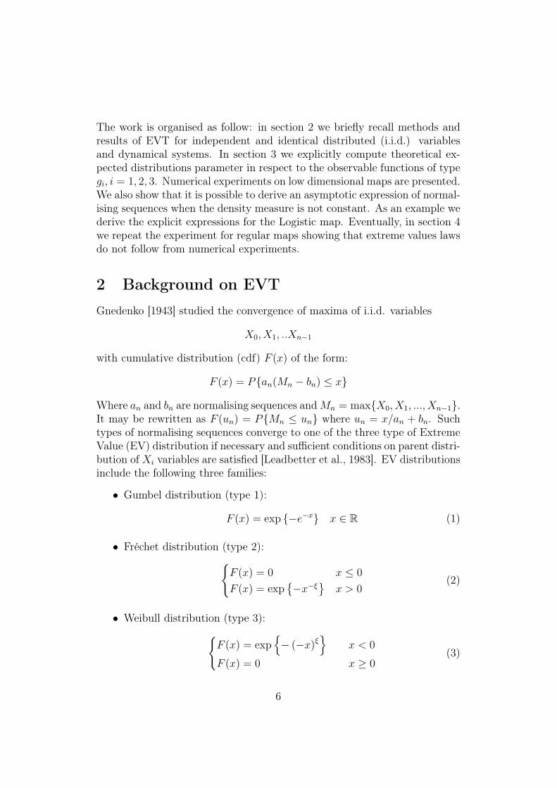
The work is organised as follow: in section 2 we briefly recall methods andresults of EVT for independent and identical distributed (i.i.d.) variablesand dynamical systems. In section 3 we explicitly compute theoretical ex-pected distributions parameter in respect to the observable functions of typegi, i = 1, 2, 3. Numerical experiments on low dimensional maps are presented.We also show that it is possible to derive an asymptotic expression of normal-ising sequences when the density measure is not constant. As an example wederive the explicit expressions for the Logistic map. Eventually, in section 4we repeat the experiment for regular maps showing that extreme values lawsdo not follow from numerical experiments.
2 Background on EVTGnedenko [1943] studied the convergence of maxima of i.i.d. variables
X0, X1, ..Xn−1
with cumulative distribution (cdf) F (x) of the form:
F (x) = Pan(Mn − bn) ≤ x
Where an and bn are normalising sequences andMn = maxX0, X1, ..., Xn−1.It may be rewritten as F (un) = PMn ≤ un where un = x/an + bn. Suchtypes of normalising sequences converge to one of the three type of ExtremeValue (EV) distribution if necessary and sufficient conditions on parent distri-bution of Xi variables are satisfied [Leadbetter et al., 1983]. EV distributionsinclude the following three families:
• Gumbel distribution (type 1):
F (x) = exp −e−x x ∈ R (1)
• Fréchet distribution (type 2):F (x) = 0 x ≤ 0
F (x) = exp−x−ξ
x > 0
(2)
• Weibull distribution (type 3):F (x) = exp
− (−x)ξ
x < 0
F (x) = 0 x ≥ 0(3)
6
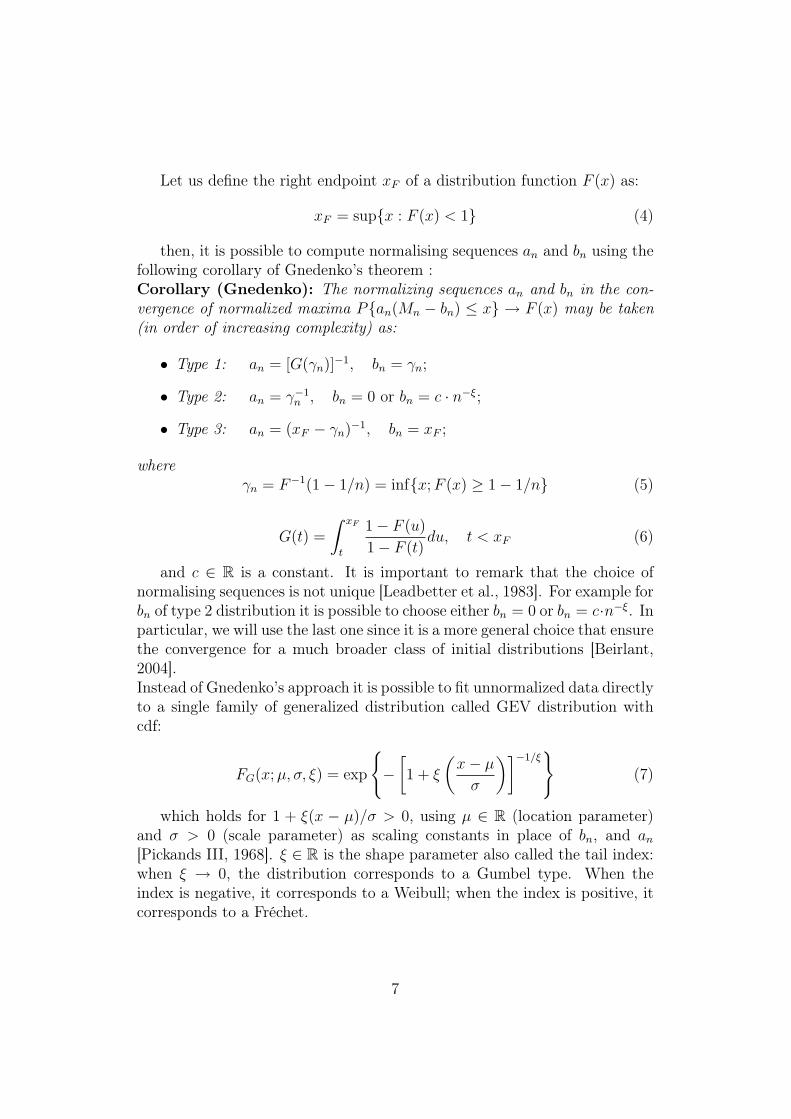
Let us define the right endpoint xF of a distribution function F (x) as:
xF = supx : F (x) < 1 (4)
then, it is possible to compute normalising sequences an and bn using thefollowing corollary of Gnedenko’s theorem :Corollary (Gnedenko): The normalizing sequences an and bn in the con-vergence of normalized maxima Pan(Mn − bn) ≤ x → F (x) may be taken(in order of increasing complexity) as:
• Type 1: an = [G(γn)]−1, bn = γn;
• Type 2: an = γ−1n , bn = 0 or bn = c · n−ξ;
• Type 3: an = (xF − γn)−1, bn = xF ;
whereγn = F−1(1− 1/n) = infx;F (x) ≥ 1− 1/n (5)
G(t) =
∫ xF
t
1− F (u)
1− F (t)du, t < xF (6)
and c ∈ R is a constant. It is important to remark that the choice ofnormalising sequences is not unique [Leadbetter et al., 1983]. For example forbn of type 2 distribution it is possible to choose either bn = 0 or bn = c·n−ξ. Inparticular, we will use the last one since it is a more general choice that ensurethe convergence for a much broader class of initial distributions [Beirlant,2004].Instead of Gnedenko’s approach it is possible to fit unnormalized data directlyto a single family of generalized distribution called GEV distribution withcdf:
FG(x;µ, σ, ξ) = exp
−[1 + ξ
(x− µσ
)]−1/ξ
(7)
which holds for 1 + ξ(x − µ)/σ > 0, using µ ∈ R (location parameter)and σ > 0 (scale parameter) as scaling constants in place of bn, and an[Pickands III, 1968]. ξ ∈ R is the shape parameter also called the tail index:when ξ → 0, the distribution corresponds to a Gumbel type. When theindex is negative, it corresponds to a Weibull; when the index is positive, itcorresponds to a Fréchet.
7

In order to adapt the extreme value theory to dynamical systems, we willconsider the stationary stochastic process X0, X1, ... given by:
Xn(x) = g(dist(fn(x), ζ)) ∀n ∈ N (8)where ’dist’ is a Riemannian metric on Ω, ζ is a given point and g is an
observable function, and whose partial maximum is defined as:
Mn = maxX0, ..., Xn−1 (9)The probability measure will be here the invariant measure ν for the
dynamical system. As we anticipated in the Introduction, we will use threetypes of observables gi, i = 1, 2, 3, suitable to obtain one of the three typesof EV distribution for normalised maxima:
g1(x) = − log(dist(x, ζ)) (10)
g2(x) = dist(x, ζ)−1/α (11)
g3(x) = C − dist(x, ζ)1/α (12)where C is a constant and α > 0 ∈ R.
These three types of functions are representatives of broader classes which aredefined, for instance, throughout equations (1.11) to (1.13) in Freitas et al.[2009]. It is easy to understand where they arise. The Gnedenko corollarysays that the different kinds of extreme value laws are determined by thedistribution of F (u) = ν(X0 ≤ u) and by the right endpoint of F , xF . Wewill see in the next section that the local invertibility of gi, i = 1, 2, 3 inthe neighborhood of 0 together with the Lebesgue’s differentiation theorem(which basically says that whenever the measure ν is absolutely continuouswith respect to Lebesgue with density ρ, the the measure of a ball of radius δcentered around almost any point x0 scales like δρ(x0)), allow us to computethe tail of F and according to this tail one will have the three types of extremelaws. At this regard let us compare Th. 1.6.2. in Leadbetter et al. [1983]with formulas (1.11)-(1.13) in Freitas et al. [2009]: one see immediately howand why the assumptions for the gi translate into similar conditions for thethree different types of asymptotic behavior for the distribution function F .
3 Extreme distributions in mixing mapsOur goal is to use a block-maxima approach and fit our unnormalised datato a GEV distribution; for that it will be necessary to find a linkage among
8
an, bn, µ and σ. At this regard we will use Gnedenko’s corollary to computenormalising sequences showing that they correspond to the parameter weobtain fitting directly data to GEV distribution.
We derive the correct expression for mixing maps with constant densitymeasure and the asymptotic behavior for logistic map that is a case of non-constant density measure.
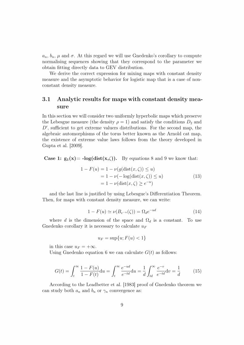
3.1 Analytic results for maps with constant density mea-sure
In this section we will consider two uniformly hyperbolic maps which preservethe Lebesgue measure (the density ρ = 1) and satisfy the conditions D2 andD′, sufficient to get extreme valuers distributions. For the second map, thealgebraic automorphisms of the torus better known as the Arnold cat map,the existence of extreme value laws follows from the theory developed inGupta et al. [2009].
Case 1: g1(x)= -log(dist(x,ζ)). By equations 8 and 9 we know that:
1− F (u) = 1− ν(g(dist(x, ζ)) ≤ u)
= 1− ν(− log(dist(x, ζ)) ≤ u)
= 1− ν(dist(x, ζ) ≥ e−u)
(13)
and the last line is justified by using Lebesgue’s Differentiation Theorem.Then, for maps with constant density measure, we can write:
1− F (u) ' ν(Be−u(ζ)) = Ωde−ud (14)
where d is the dimension of the space and Ωd is a constant. To useGnedenko corollary it is necessary to calculate uF
uF = supu;F (u) < 1
in this case uF = +∞.Using Gnedenko equation 6 we can calculate G(t) as follows:
G(t) =
∫ ∞t
1− F (u)
1− F (t)du =
∫ ∞t
e−ud
e−tddu =
1
d
∫ ∞td
e−v
e−tddv =
1
d(15)
According to the Leadbetter et al. [1983] proof of Gnedenko theorem wecan study both an and bn or γn convergence as:
9
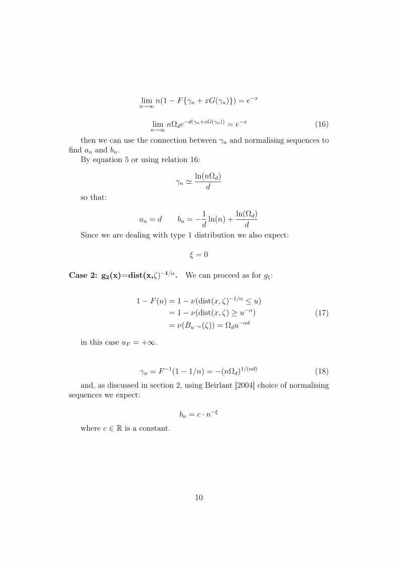
limn→∞
n(1− Fγn + xG(γn)) = e−x
limn→∞
nΩde−d(γn+xG(γn)) = e−x (16)
then we can use the connection between γn and normalising sequences tofind an and bn.
By equation 5 or using relation 16:
γn 'ln(nΩd)
d
so that:
an = d bn = −1
dln(n) +
ln(Ωd)
d
Since we are dealing with type 1 distribution we also expect:
ξ = 0
Case 2: g2(x)=dist(x,ζ)−1/α. We can proceed as for g1:
1− F (u) = 1− ν(dist(x, ζ)−1/α ≤ u)
= 1− ν(dist(x, ζ) ≥ u−α)
= ν(Bu−α(ζ)) = Ωdu−αd
(17)
in this case uF = +∞.
γn = F−1(1− 1/n) = −(nΩd)1/(αd) (18)
and, as discussed in section 2, using Beirlant [2004] choice of normalisingsequences we expect:
bn = c · n−ξ
where c ∈ R is a constant.
10
Case 3: g3(x)=C-dist(x,ζ)1/α. Eventually we compute an and bn for theg3 observable class:
1− F (u) = 1− ν(C − dist(x, ζ)1/α ≤ u)
= 1− ν(dist(x, ζ) ≥ (C − u)α)
= ν(B(C−u)α(ζ)) = Ωd(C − u)αd(19)
in this case uF = C.
γn = F−1(1− 1/n) = C − (nΩd)1/(αd) (20)
For type 3 distribution:
an = (uF − γn)−1, bn = uF ; (21)
3.2 Numerical Experiments for Maps with constant den-sity measure
Since we want to show that unnormalised data may be fitted by using theGEV distribution FG(x;µ, σ, ξ) we expect to find the following equivalence:
an = 1/σ bn = µ
where, clearly, µ = µ(n) and σ = σ(n). This fact can be seen as a linearchange of variable: the variable y = an(x − bn) has a GEV distributionFG(y;µ = 0, σ = 1, ξ) (that is an EV one parameter distribution with anand bn normalising sequences) while x is GEV distributed FG(x;µ = bn, σ =1/an, ξ).
As we said above we now apply the previous considerations to two mapswhich enjoy extreme values laws and have constant density: we summarizebelow the theoretical results we obtained for all three type of observables.
For g1 type observable:
σ =1
dµ ∝ −1
dln(n) (22)
For g2 type observable:
σ ∝ −n1/(αd) µ ∝ −n1/(αd) (23)
For g3 type observable:
11
σ ∝ n1/(αd) µ = C (24)
The one-dimensional map used is a Bernoulli Shift map:
xt+1 = qxt mod 1 q > 1 ∈ N (25)
with q = 3.
By comparing with the form of the GEV (eq. (7)) we also know the valuesof shape parameter ξ. It has to be ξ = 0 for g1 type , ξ = 1/(αd) for g2 typeand ξ = −1/(αd) for g3 type.
We now consider the Arnold’s cat map defined on the 2-torus by:[xt+1
yt+1
]=
[2 11 1
] [xtyt
]mod 1 (26)
A wide description of properties of these maps can be found in Arnoldand Avez [1968] and Hasselblatt and Katok [2003].
All the numerical analysis contained in this work has been performed us-ing MATLAB Statistics Toolbox functions such as gevfit and gevcdf. Thesefunctions return maximum likelihood estimates of the parameters for thegeneralized extreme value (GEV) distribution giving 95% confidence inter-vals for estimates [Martinez and Martinez, 2002].For each observable function gi i = 1, 2, 3 we have done k = 107 iterationsfor both maps starting from different initial conditions ζ. The results wepresent don’t depend on the choice of initial point except for some trivialinitial conditions. The method of maximum likelihood selects values of themodel parameters that produce the distribution most likely to have resultedin the observed data. Since we have a strong theoretical models for our obser-vations that is we expect to find a well defined GEV distribution this fittingprocedure seems appropriate to check the experimental data distribution.Once the series of observables is divided into n bins each containing m = k/nobservations, and the maximum value of gi is taken in each bin, the unnor-malised maxima have been fitted to GEV distribution FG(x;µ, σ, ξ) for dif-ferent (n, k/n) combinations. In every case considered, fitted distributionspassed, with maximum confidence interval, the Kolmogorov-Smirnov test de-scribed in Lilliefors [1967].Numerical data let us check two different limiting behaviors:
• The limit in which n is small (few maxima taken within intervals con-taining many iterations of maps).
12
• The limit in which intervals contain few iterations of maps but with awide number of maxima n .
Regarding n we have in general that in order to obtain a reliable fit fora distribution with p parameters we need 10p independent data [Felici et al.,2007a] so that we expect that fit procedure gives reliable results for n > 103,while the lower bound on m depends on the ability to select proper extremevalues in a bin that contains a consistent number of observations. In thelatter case we have no a priori estimations on the magnitude of m but wecan study it numerically against theoretical parameters.
For a g1 type observable function the behavior against n of the threeparameters is presented in figure 1. According to equation 22 we expect tofind ξ = 0. For relatively small values of n the sample is too small to ensurea good convergence to analytical ξ and confidence intervals are wide. Onthe other hand we see deviations from expected value as m < 103 that iswhen n > 104. For the scale parameter a similar behavior is achieved anddeviations from expected theoretical values σ = 1/2 for Arnold Cat Map andσ = 1 for Bernoulli Shift are found when n < 103 or m < 103. Locationparameter µ shows a logarithm decay with n as expected from equation 22.A linear fit of µ in respect to log(n) is shown with a red line in figure 1. Thelinear fit computed angular coefficients K∗ of equation 22 well approximate1/d: for Bernoulli Shift map we obtain |K∗| = 1.001±0.001 while for ArnoldCat map |K∗| = 0.489 ± 0.001. We find that ξ values have best matchingwith theoretical ones with reliable confidence interval when both n > 103
and m > 103. These results are confirmed even for g2 type and g3 type ob-servable functions as shown in figures 2a) and 3a) respectively. We presentthe fit results for α = 3 but we have done tests for different α and for fixedn and different α.For g2 observable function we can also check that µ and σ parameters followa power law as described in eq. 23. In the log-log plot in Figure 2b), 2c), wecan see a very clear linear behavior. For the Bernoulli Shift map we obtain|K∗| = 0.330± 0.001 for µ series , |K∗| = 0.341± 0.001 for σ in good agree-ment with theoretical value of 1/3. For Arnold Cat map we expect to findK∗ = 1/6, from the experimental data we obtain |K∗| = 0.163± 0.001 for µand |K∗| = 0.164± 0.001 for σ.Eventually, computing g3 as observable function we expect to find a constantvalue for µ while σ has to grow with a power law in respect to n as expectedfrom equation 24. As in g2 case we expect |K∗| = 1/(αd) and numericalresults shown in figure 3b), 3c) are consistent with the theoretical one since|K∗| = 0.323 ± 0.006 for Bernoulli shift map and |K∗| = 0.162 ± 0.006 for
13
Arnold Cat map.
In all cases considered the analytical behavior described in equation 23and 24 is achieved and the fit quality improves if n > 103 and m > 103. Theg3 type observable constant has been chosen C = 10. The nature of theselower bound is quite different:
3.3 Asymptotic sequences for maps with non-constantdensity measure
The main problem when dealing with maps that have absolutely continuousbut non-constant density measure ρ(ζ) is in the computation of the integral:
ν(Bδ(ζ)) =
∫Bδ(ζ)
ρ(ζ)dζ (27)
where Bδ(ζ) is the d-dimensional ball of radius δ centered in ζ.We have to know the value of this integral in order to evaluate F (u) and,therefore, the sequences an and bn.As shown in the previous section δ is linked to the observable type: in allcases, since we substitute u = 1 − 1/n, δ → 0 means that we are interestedin n→∞.In this limit, a first order approximation of the previous integral is:
ν(Bδ(ζ)) ' ρ(ζ)δd +O(δd+1) (28)
that is valid if we are not in a neighborhood of a singular point of ρ(ζ).
As an example we compute the asymptotic sequences for a logistic map:
xt+1 = rxt(1− xt) (29)
with r = 4. This map satisfies hypothesis described in the analysis per-formed for Benedicks-Carleson maps in Moreira Freitas and Freitas [2008].
For this map the density of the absolutely continuous invariant measureis explicit and reads:
ρ(ζ) =1
π√ζ(1− ζ)
ζ ∈ (0, 1) (30)
So that:
14
∫Bδ(ζ)
ρ(ζ)dζ =2
π
[arcsin(
√ζ + δ − arcsin(
√ζ − δ
](31)
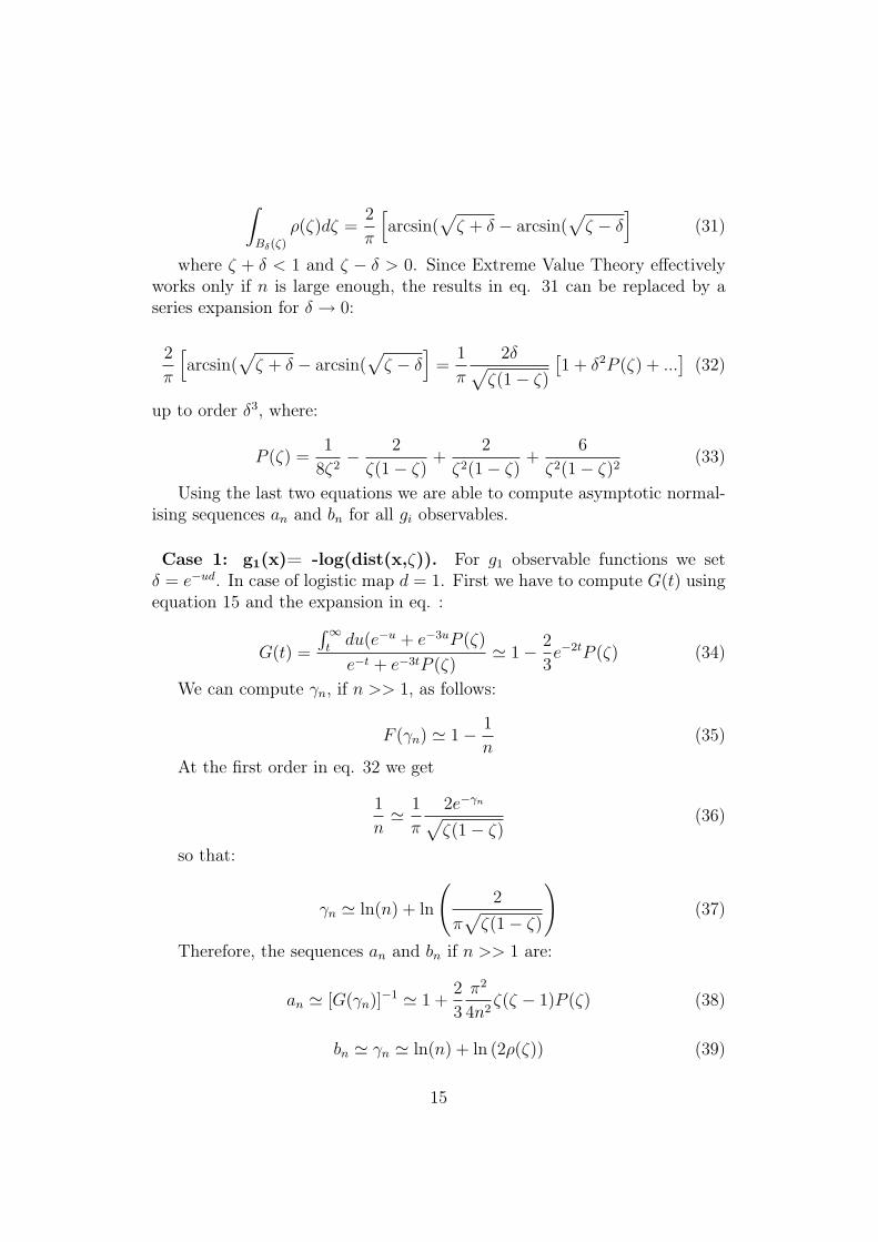
where ζ + δ < 1 and ζ − δ > 0. Since Extreme Value Theory effectivelyworks only if n is large enough, the results in eq. 31 can be replaced by aseries expansion for δ → 0:
2
π
[arcsin(
√ζ + δ − arcsin(
√ζ − δ
]=
1
π
2δ√ζ(1− ζ)
[1 + δ2P (ζ) + ...
](32)
up to order δ3, where:
P (ζ) =1
8ζ2− 2
ζ(1− ζ)+
2
ζ2(1− ζ)+
6
ζ2(1− ζ)2(33)
Using the last two equations we are able to compute asymptotic normal-ising sequences an and bn for all gi observables.
Case 1: g1(x)= -log(dist(x,ζ)). For g1 observable functions we setδ = e−ud. In case of logistic map d = 1. First we have to compute G(t) usingequation 15 and the expansion in eq. :
G(t) =
∫∞tdu(e−u + e−3uP (ζ)
e−t + e−3tP (ζ)' 1− 2
3e−2tP (ζ) (34)
We can compute γn, if n >> 1, as follows:
F (γn) ' 1− 1
n(35)
At the first order in eq. 32 we get
1
n' 1
π
2e−γn√ζ(1− ζ)
(36)
so that:
γn ' ln(n) + ln
(2
π√ζ(1− ζ)
)(37)
Therefore, the sequences an and bn if n >> 1 are:
an ' [G(γn)]−1 ' 1 +2
3
π2
4n2ζ(ζ − 1)P (ζ) (38)
bn ' γn ' ln(n) + ln (2ρ(ζ)) (39)
15
Case 2: g2(x)=dist(x,ζ)−1/α. We can proceed as for g1 setting δ =(αu)−α, computing γn we get at the first order in eq. 32:
1
n' 1
π
2γ−αn√ζ(1− ζ)
= 2ρ(ζ)(αγn)−α (40)
γn =1
α
(1
2nρ(ζ)
)−1/α
(41)
We can respectively compute an and bn as:
an = γ−1n bn = (2nρ(ζ))ξ (42)
Case 3: g3(x)=C-dist(x,ζ)1/α. As in the previous cases, we compute γnup to the first order setting δ = [α(C − γn)]α:
1
n' 1
π
2[α(C − γn)]α√ζ(1− ζ)
= 2ρ(ζ)[α(C − γn)]α (43)
γn = C − 1
α
(1
2nρ(ζ)
)1/α
(44)
For type 3 distribution:
an = (uF − γn)−1, bn = uF ; (45)
where uf = C.
3.4 Numerical experiment on the logistic map
We want to show the equivalence between EV computed normalising se-quences an and bn and the parameters of a GEV distribution obtained di-rectly fitting the data even in case of logistic map that has not constantdensity measure. Using eq. 38-39 for g1 we obtain the following theoreticalexpression:
σ(n, ζ) ' 1 +2
3
π2
4n2ζ(ζ − 1)P (ζ) µ(n, ζ) ' ln(n) + ln(2ρ(ζ)) (46)
From eq. 39, for g2 observable type, we write:
σ(n, ζ) ' 1
α(2nρ(ζ))
1α µ(n, ζ) ' (2nρ(ζ))
1α (47)
16

and in g3 case using eq. 45, we expect to find:
σ(n, ζ) ' 1
α(2nρ(ζ))−1/α µ(n, ζ) ' C = uF (48)
Values of ξ are independent on density and, as stated in Freitas’ ξ = 0for g1 type , ξ = 1/(αd) for g2 type and ξ = −1/(αd) for g3 type.
In figures 4-6 we presents a numerical test of the asymptotic behavior de-scribed in equations 46 - 48 on logistic map for d = 1 , a = 3, C = uF = 10,ζ = 0.3 and variable n. As shown in previous section, block maxima ap-proach works well with maps with constant density measure when n and mare at least 103: In fact, regarding ξ parameter. Significant deviations fromthe theoretical value are achieved when n < 1000 or m < 1000 even in thecase of the Logistic Map.Regarding µ and σ, for g1 observable a linear fit of µ in respect to log(n)give us |K∗| = 0.999± 0.002, while σ shows the same behavior of ξ since thebest agreement with theoretical value σ = 1 is achieved when n,m > 103.In the log-log plots of figure 5b), 5c) for g2 observable, we can observeagain the expected linear behavior for µ and σ with |K∗| corresponding to1/(αd). From numerical fit we obtain |K∗| = 0.3334 ± 0.0007 for µ seriesand |K∗| = 0.337 ± 0.002 for σ in good agreement with theoretical value of1/3. By applying a linear fit to the log-log plot in figure 6b), the angularcoefficient corresponding to σ series is |K| = 0.323 ± 0.003 again consistentwith the theory.
For a logistic map we can also check the GEV behavior in respect to initialconditions. If we fix n∗ = m∗ = 103 and fit our data to GEV distribution for103 different ζ ∈ (0, 1) an asymptotic behavior is reached as shown from theprevious analysis. For g1 observable function we have observed that the firstorder approximation works well for all three parameters. Deviation from thisbehavior are achieved for ζ → 1 and ζ → 0 as the measure become singularwhen we move to these points and we should take in account other terms ofthe series expansion. Numerically, we found that deviations from first orderapproximation are meaningful only if ζ < 10−3 and ζ > 1− 10−3. Averagingover ζ both ξ and σ we obtain < ξ >= 1.000±0.009 and < σ >= 1.00±0.03where the uncertainties are computed with respect to the estimator. Sincewe expect ξ = 0 and σ = 1 at zero order approximation, numerical resultsare consistent with the theoretical ones; furthermore, experimental data arenormally distributed around theoretical values.Asymptotic expansion also works well for g2 observables: we obtain < ξ >=0.334 ± 0.001 in excellent agreement with theoretical value ξ = 1/3. Even-
17

tually, in g3, averaging ξ over different initial conditions we get < ξ >=−0.334± 0.002 that is again consistent to theoretical value -1/3.
4 Extreme distributions in regular mapsFreitas and Freitas [2008] have posed the problem of dependent extreme val-ues in dynamical systems that show uniform quasi periodic motion. Here wetry to investigate this problem numerically. We have used a one-dimensionaland a bi-dimensional discrete map. The first one is the irrational translationon the torus defined by:
xt+1 = xt + β mod 1 β ∈ [0, 1] \Q (49)
And for the bidimensional case, we use the so called standard map:
yt+1 = yt +λ
2πsin(2πxt) mod 1; xt+1 = xt + yt+1 mod 1. (50)
with λ = 10−4. For this value of λ, the standard map exhibits a regularbehavior and it is not mixing, as well as torus translations. This means thatthese maps fail in satisfying hypothesis D2 and D′ and moreover they do notenjoy as well an exponential hitting time statistics. About this latter statis-tics, it is however known that it exists for torus translation and it is givenby a particular piecewise linear function or a uniform distribution dependingon which sequence of sets Ak is considered [Coelho and De Faria, 1996]. Ina similar way, a non-exponential HTS is achieved for standard map whenλ << 1 as well as for a skew map, that is a standard map with λ = 0 [Buricet al., 2005]. Therefore we expect not to obtain a GEV distribution of anytype using gi observables.
We have pointed out that the observable functions choice is crucial inorder to observe some kind of distribution of extreme values when we aredealing with dynamical systems instead of stochastic series. Nicolis et al.[2006] have shown how it is possible to obtain an analytical EV distributionwhich does not belong to GEV family choosing a simple observable: theyconsidered the series of distances between the iterated trajectory and theinitial condition. Using the same notation of section 2 we can write:
Yn(x = f tζ) = dist(f tζ, ζ) Mn = minY0, ...Yn−1For this observable they have shown that the cumulative distribution
F (x) = Pan(Mn − bn) ≤ x of a uniform quasi periodic motions is not
18

smooth but piecewise linear (Nicolis et al. [2006], figure 3). Furthermore slopchanges of F (x) can be explained by constructing the intersections betweendifferent iterates of equation 49. F (x) must correspond to a density distribu-tion continuous obtained as a composition of box functions: each box mustbe related to a change in the slope of F (x).
The numerical results we report below confirm that for the maps 49 and50 the distributions of maxima for various observables cannot be fitted witha GEV since they are multi modal. We recall that the return times into asphere of vanishing radius do not have a spectrum, if the orbits have the samefrequency, whereas a spectrum appears if the frequency varies continuouslywith the action, as in the standard map for λ close to zero [Hu et al., 2004].Since the EV statistics refers to a single orbit, no change due to the localmixing, which insures the existence of a return times spectrum [Hu et al.,2004], can be observed. Considering that the GEV exists when the systemis mixing and does not when it is integrable, one might use the quality offit to GEV as a dynamical indicator, for systems which exhibit regions withdifferent dynamical properties, ranging from integrable to mixing as it occursfor the standard map when λ is order 1. Indeed we expect that in the neigh-borhood of a low order resonance, where the omoclinic tangle of intersectingseparatrices appears, a GEV fit is possible. Preliminary computations car-ried out for the standard map and for a model with parametric resonanceconfirm this claim, that will be carefully tested in the near future.
Using the theoretical framework provided in Nicolis et al. [2006] we checknumerically the behavior of maps described in eq. 49-50 analysing EV dis-tributions for gi observable functions. Proceeding as in section 3 for mixingmaps, we try to perform a fit to GEV distribution starting with different ini-tial conditions ζ, a set of different α values and (n,m) combinations. In allcases analysed the Kolmogorov Smirnov test fails and this means that GEVdistribution is not useful to describe the behavior of this kind of statistics.This result is in agreement with Freitas et al. [2010b] but we may find outwhich kind of empirical distribution is obtained.
Looking in details atMn histograms that correspond to empirical densitydistributions, they appear always to be multi modal and each mode have awell defined shape: for g1 type observable function modes are exponentialwhile, for g2 and g3, their shape depends on α value of observable function.Furthermore, the number of modes and their positions are highly dependenton both n and initial conditions.Using Nicolis et al. [2006] results it is possible to understand why we obtain
19
this kind of histograms: since density distribution of Mn is a compositionof box functions, when we apply gi observables we modulate it changing theshape of the boxes. Therefore, we obtain a multi modal distribution modifiedaccording to the observable functions gi.An example is shown in figure 7 for standard map: the left figures correspondto the histogram of the minimum distance obtained without computing giobservable and reproduce a composition of box functions. The figures in theright show how this distribution is modified by applying g1 observable to theseries of minimum distances. We can see two exponential modes, while thethird is hidden in the linear scale but can be highlighted using a log-scale.The upper figures are drawn using n = 3300, m = 3300, the lower withn = 10000, m = 1000.
5 Concluding RemarksEVT was developed to study a wide class of problems of great interest indifferent disciplines: the need of modeling events that occur with very smallprobability comes from the fact that they can affect in a strong way severalsocioeconomic activities: floods, insurance losses, earthquakes, catastrophes.It was applied on limited data series using the block-maxima approach fac-ing the problem of having a good statistics of extreme values retaining asufficient number of observation in each bin. Often, since no theoretical apriori values of GEV parameters are available for this kind of applications,we may obtain a biased fit to GEV distribution even if tests of statisticalsignificance succeed. The recent development of an extreme value theory indynamical systems give us the theoretical framework to test the consistencyof block-maxima approach when analytical results for distribution parame-ters are available.
Our main finding is that a block-maxima approach for GEV distributionis totally equivalent to fit an EV distribution after normalising sequences arecomputed. To prove this we have derived analytical expressions for an andbn normalising sequences, showing that µ and σ of fitted GEV distributioncan replace them. This approach works for maps that have an absolutelycontinuous invariant measure and retain some mixing properties that canbe directly related to the exponential decay of HTS. Since GEV approachdoes not require the a-priori knowledge of the measure density that is in-stead require by the EV approach, it is possible to use it in many numericalapplications.
20

Furthermore, if we compare analytical and numerical results we can studywhat is the minimum number of maxima and how big the set of observationsin which the maximum is taken has to be. To accomplish this goal we haveanalysed maps with constant density measure finding that a good agreementbetween numerical and analytical value is achieved when both the numberof maxima n and the observations per bin m are at least 103. We remarkthat the fits have passed Kolmogorov Smirnov test with maximum confidenceinterval even if n < 103 or < m < 103 so that parametric or non parametrictests are not the only thing to take in account when dealing with extremevalue distributions: if maxima are not proper extreme values (which meansm is not large enough) the fit is good but parameters are different from ex-pected values. The lower bound of n can be explained using the argumentthat a fit to a 3-parameters distribution needs at least 103 independent datato give reliable informations.Therefore, we checked that in case of non-constant absolutely continuousdensity measure the asymptotic expressions used to compute µ and σ workswhen we consider n and m of order 103. For logistic map the numericalvalues of parameters we obtain averaging over different initial conditions aretotally in agreement with the theoretical ones. In regular maps, as expected,the fit to a GEV distribution is unreliable. We obtain a multi modal distri-bution, that, for the analyzed maps, is the result of a composition of modesin which the shape depends on observable types. This behavior can be ex-plained pointing out that this kind of systems have not an exponential HTSdecay and therefore have no EV law for observables of type gi.
To conclude, we claim that we have provided a reliable way to investigateproperties of extreme values in mixing dynamical systems which may satisfymixing conditions (like D2 and D′), finding an equivalence among an, bn, µand σ behavior for absolutely continuous measures. In our future work weintend to address the case of singular measure. Recently the theorem wasgeneralised to the case of non smooth observations and therefore it holdsalso with non absolutely continuous invariant probability measure [Freitaset al., 2010b]. In this case we expect the same for all the procedure describedhere. Understanding the extreme values behavior for singular measures willbe crucial to apply proficiently this analysis to operative geophysical modelssince in these case we are always dealing with singular measures (for a detaileddiscussion of this issue, see Lucarini and Sarno [2011]). In this way wewill provide a complete tool to study extreme events in complex dynamicalsystems used in geophysical or financial applications. Furthermore, sincea GEV distribution for extreme values exists when the system is mixingand does not when it is integrable, in future works we will also address the
21
problem of using the quality of fit to GEV as a dynamical indicator, forsystems which exhibit regions with different dynamical properties.
6 AcknowledgmentsS.V. was supported by the CNRS-PEPS Project Mathematical Methods ofClimate Models , and he thanks the GDRE Grefi-Mefi for having supportedexchanges with Italy. V.L. and D.F. acknowledge the financial support of theEU FP7-ERC project NAMASTE “Thermodynamics of the Climate System".
22

Figure 1: g1 observable, ζ ' 0.51. a) ξ VS log10(n); b) σ VS log10(n); c) µVS log(n). Right: Bernoulli Shift map. Left: Arnold Cat Map. Dotted linesrepresent computed confidence interval, red lines represent a linear fit, bluelines are theoretical values.
23

Figure 2: g2 observable, ζ ' 0.51. a) ξ VS log10(n); b) log10(σ) VS log10(n);c) log10(µ) VS log10(n). Right: Bernoulli Shift map. Left: Arnold Cat Map.Dotted lines represent computed confidence interval, red lines represent alinear fit, blue lines are theoretical values.
24

Figure 3: g3 observable, ζ ' 0.51. a) ξ VS log10(n); b) log10(σ) VS log10(n);c) log10(µ) VS log10(n). Right: Bernoulli Shift map. Left: Arnold Cat Map.Dotted lines represent computed confidence interval, red lines represent alinear fit, blue lines are theoretical values.
25

Figure 4: g1 observable, ζ = 0.31. a) ξ VS log10(n); b) σ VS log10(n);c) µ VS log(n). Logistic map. Dotted lines represent computed confidenceinterval, red lines represent a linear fit, blue lines are theoretical values.
26

Figure 5: g2 observable, ζ = 0.3. a) ξ VS log10(n); b) log10(σ) VS log10(n);c) log10(µ) VS log10(n). Logistic map. Dotted lines represent computedconfidence interval, red lines represent a linear fit, blue lines are theoreticalvalues.
27
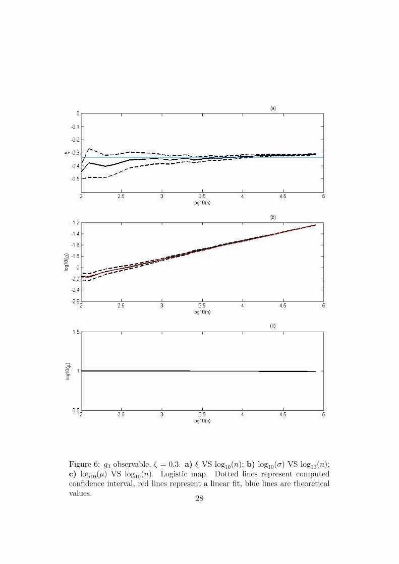
Figure 6: g3 observable, ζ = 0.3. a) ξ VS log10(n); b) log10(σ) VS log10(n);c) log10(µ) VS log10(n). Logistic map. Dotted lines represent computedconfidence interval, red lines represent a linear fit, blue lines are theoreticalvalues.
28
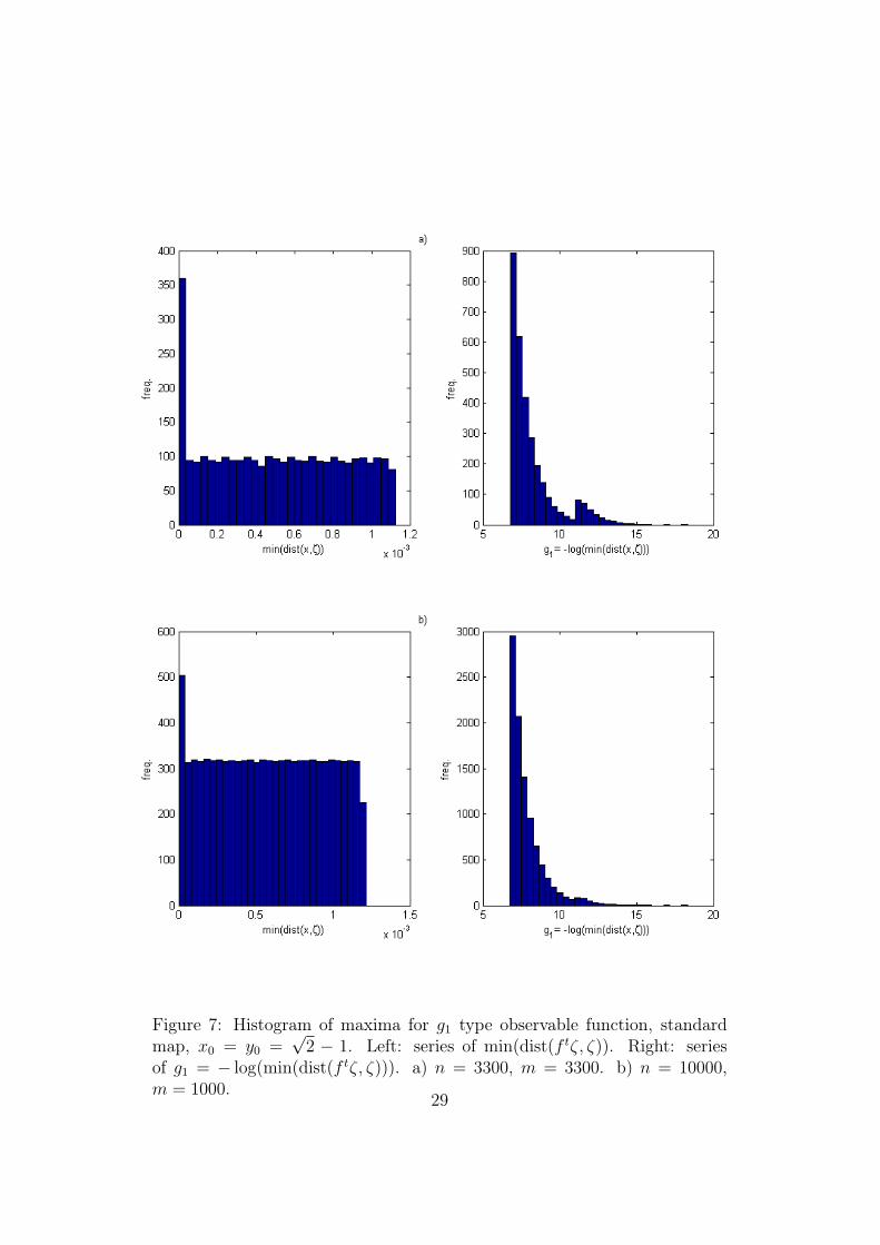
Figure 7: Histogram of maxima for g1 type observable function, standardmap, x0 = y0 =
√2 − 1. Left: series of min(dist(f tζ, ζ)). Right: series
of g1 = − log(min(dist(f tζ, ζ))). a) n = 3300, m = 3300. b) n = 10000,m = 1000.
29
ReferencesE.G. Altmann, S. Hallerberg, and H. Kantz. Reactions to extreme events:Moving threshold model. Physica A: Statistical Mechanics and its Appli-cations, 364:435–444, 2006.
V.I. Arnold and A. Avez. Ergodic problems of classical mechanics. BenjaminNew York, 1968.
V. Balakrishnan, C. Nicolis, and G. Nicolis. Extreme value distributionsin chaotic dynamics. Journal of Statistical Physics, 80(1):307–336, 1995.ISSN 0022-4715.
J. Beirlant. Statistics of extremes: theory and applications. John Wiley &Sons Inc, 2004. ISBN 0471976474.
E. Bertin. Global fluctuations and Gumbel statistics. Physical review letters,95(17):170601, 2005. ISSN 1079-7114.
E. Brodin and C. Kluppelberg. Extreme Value Theory in Finance. Submittedfor publication: Center for Mathematical Sciences, Munich University ofTechnology, 2006.
N. Buric, A. Rampioni, and G. Turchetti. Statistics of Poincaré recurrencesfor a class of smooth circle maps. Chaos, Solitons & Fractals, 23(5):1829–1840, 2005.
P.W. Burton. Seismic risk in southern Europe through to India examinedusing Gumbel’s third distribution of extreme values. Geophysical Journalof the Royal Astronomical Society, 59(2):249–280, 1979. ISSN 1365-246X.
M. Clusel and E. Bertin. Global fluctuations in physical systems: a subtleinterplay between sum and extreme value statistics. International Journalof Modern Physics B, 22(20):3311–3368, 2008. ISSN 0217-9792.
Z. Coelho and E. De Faria. Limit laws of entrance times for homeomorphismsof the circle. Israel Journal of Mathematics, 93(1):93–112, 1996. ISSN0021-2172.
S. Coles, J. Heffernan, and J. Tawn. Dependence measures for extreme valueanalyses. Extremes, 2(4):339–365, 1999. ISSN 1386-1999.
P. Collet. Statistics of closest return for some non-uniformly hyperbolic sys-tems. Ergodic Theory and Dynamical Systems, 21(02):401–420, 2001. ISSN0143-3857.
30
C.A. Cornell. Engineering seismic risk analysis. Bulletin of the SeismologicalSociety of America, 58(5):1583, 1968. ISSN 0037-1106.
M.G. Cruz. Modeling, measuring and hedging operational risk. John Wiley& Sons, 2002. ISBN 0471515604.
K. Dahlstedt and H.J. Jensen. Universal fluctuations and extreme-valuestatistics. Journal of Physics A: Mathematical and General, 34:11193,2001.
A.C. Davison. Modelling excesses over high thresholds, with an application.Statistical Extremes and Applications, pages 461–482, 1984.
AC Davison and R.L. Smith. Models for exceedances over high thresholds.Journal of the Royal Statistical Society. Series B (Methodological), 52(3):393–442, 1990. ISSN 0035-9246.
P. Embrechts, S.I. Resnick, and G. Samorodnitsky. Extreme value theoryas a risk management tool. North American Actuarial Journal, 3:30–41,1999. ISSN 1092-0277.
M. Felici, V. Lucarini, A. Speranza, and R. Vitolo. Extreme Value Statisticsof the Total Energy in an Intermediate Complexity Model of the Mid-latitude Atmospheric Jet. Part I: Stationary case.(3337K, PDF). Journalof Atmospheric Science, 64:2137–2158, 2007a.
M. Felici, V. Lucarini, A. Speranza, and R. Vitolo. Extreme value statisticsof the total energy in an intermediate complexity model of the mid-latitudeatmospheric jet. Part II: trend detection and assessment. Journal of At-mospheric Science, 64:2159–2175, 2007b.
RA Fisher and LHC Tippett. Limiting forms of the frequency distributionof the largest or smallest member of a sample. In Proceedings of the Cam-bridge philosophical society, volume 24, page 180, 1928.
A.C.M. Freitas and J.M. Freitas. On the link between dependence and in-dependence in extreme value theory for dynamical systems. Statistics &Probability Letters, 78(9):1088–1093, 2008. ISSN 0167-7152.
A.C.M. Freitas, J.M. Freitas, and M. Todd. Hitting time statistics and ex-treme value theory. Probability Theory and Related Fields, pages 1–36,2009.
A.C.M. Freitas, J.M. Freitas, and M. Todd. Extremal Index, Hitting TimeStatistics and periodicity. Arxiv preprint arXiv:1008.1350, 2010a.
31
A.C.M. Freitas, J.M. Freitas, M. Todd, B. Gardas, D. Drichel, M. Flohr,RT Thompson, SA Cummer, J. Frauendiener, A. Doliwa, et al. Ex-treme value laws in dynamical systems for non-smooth observations. Arxivpreprint arXiv:1006.3276, 2010b.
M. Gilli and E. Këllezi. An application of extreme value theory for measuringfinancial risk. Computational Economics, 27(2):207–228, 2006. ISSN 0927-7099.
B. Gnedenko. Sur la distribution limite du terme maximum d’une sériealéatoire. The Annals of Mathematics, 44(3):423–453, 1943.
EJ Gumbel. The return period of flood flows. The Annals of MathematicalStatistics, 12(2):163–190, 1941. ISSN 0003-4851.
C. Gupta. Extreme-value distributions for some classes of non-uniformlypartially hyperbolic dynamical systems. Ergodic Theory and DynamicalSystems, 30(03):757–771, 2010. ISSN 0143-3857.
C. Gupta, M. Holland, and M. Nicol. Extreme value theory for hyperbolicbilliards. Lozi-like maps, and Lorenz-like maps, preprint, 2009.
G. Haiman. Extreme values of the tent map process. Statistics & ProbabilityLetters, 65(4):451–456, 2003. ISSN 0167-7152.
S. Hallerberg and H. Kantz. Influence of the event magnitude on the pre-dictability of an extreme event. Physical Review E, 77(1):11108, 2008.ISSN 1550-2376.
B. Hasselblatt and AB Katok. A first course in dynamics: with a panoramaof recent developments. Cambridge Univ Pr, 2003.
B.M. Hill. A simple general approach to inference about the tail of a distri-bution. The Annals of Statistics, 3(5):1163–1174, 1975. ISSN 0090-5364.
M. Holland, M. Nicol, and A. Török. Extreme value distributions for non-uniformly hyperbolic dynamical systems. preprint, 2008.
H. Hu, A. Rampioni, L. Rossi, G. Turchetti, and S. Vaienti. Statistics ofPoincaré recurrences for maps with integrable and ergodic components.Chaos: An Interdisciplinary Journal of Nonlinear Science, 14:160, 2004.
H. Kantz, E. Altmann, S. Hallerberg, D. Holstein, and A. Riegert. Dynamicalinterpretation of extreme events: predictability and predictions. Extremeevents in nature and society, pages 69–93, 2006.
32

RW Katz. Extreme value theory for precipitation: Sensitivity analysis forclimate change. Advances in Water Resources, 23(2):133–139, 1999. ISSN0309-1708.
R.W. Katz and B.G. Brown. Extreme events in a changing climate: vari-ability is more important than averages. Climatic change, 21(3):289–302,1992. ISSN 0165-0009.
R.W. Katz, G.S. Brush, and M.B. Parlange. Statistics of extremes: Modelingecological disturbances. Ecology, 86(5):1124–1134, 2005. ISSN 0012-9658.
MR Leadbetter, G. Lindgren, and H. Rootzen. Extremes and related proper-ties of random sequences and processes. Springer, New York, 1983.
H.W. Lilliefors. On the Kolmogorov-Smirnov test for normality with meanand variance unknown. Journal of the American Statistical Association,62(318):399–402, 1967. ISSN 0162-1459.
F.M. Longin. From value at risk to stress testing: The extreme value ap-proach. Journal of Banking & Finance, 24(7):1097–1130, 2000. ISSN0378-4266.
V. Lucarini and S. Sarno. A Statistical Mechanical Approach for the Com-putation of the Climatic Response to General Forcings . Nonlin. ProcessesGeophys, 2011.
W.L. Martinez and A.R. Martinez. Computational statistics handbook withMATLAB. CRC Press, 2002.
E.S. Martins and J.R. Stedinger. Generalized maximum-likelihood gener-alized extreme-value quantile estimators for hydrologic data. Water Re-sources Research, 36(3):737–744, 2000. ISSN 0043-1397.
A.C. Moreira Freitas and J.M. Freitas. Extreme values for Benedicks–Carleson quadratic maps. Ergodic Theory and Dynamical Systems, 28(04):1117–1133, 2008. ISSN 0143-3857.
N. Nicholis. CLIVAR and IPCC interests in extreme events’. In WorkshopProceedings on Indices and Indicators for Climate Extremes, Asheville,NC. Sponsors, CLIVAR, GCOS and WMO, 1997.
C. Nicolis, V. Balakrishnan, and G. Nicolis. Extreme events in deterministicdynamical systems. Physical review letters, 97(21):210602, 2006. ISSN1079-7114.
33

Friederichs P. and A. Hense. Statistical downscaling of extreme precipitationevents using censored quantile regression. Monthly weather review, 135(6):2365–2378, 2007. ISSN 0027-0644.
J. Pickands III. Moment convergence of sample extremes. The Annals ofMathematical Statistics, 39(3):881–889, 1968.
J. Pickands III. Statistical inference using extreme order statistics. the Annalsof Statistics, pages 119–131, 1975. ISSN 0090-5364.
R.L. Smith. Threshold methods for sample extremes. Statistical extremesand applications, 621:638, 1984.
R.L. Smith. Extreme value analysis of environmental time series: an appli-cation to trend detection in ground-level ozone. Statistical Science, 4(4):367–377, 1989. ISSN 0883-4237.
D. Sornette, L. Knopoff, YY Kagan, and C. Vanneste. Rank-ordering statis-tics of extreme events: application to the distribution of large earthquakes.Journal of Geophysical Research, 101(B6):13883, 1996. ISSN 0148-0227.
O.G.B. Sveinsson and D.C. Boes. Regional frequency analysis of extreme pre-cipitation in northeastern colorado and fort collins flood of 1997. Journalof Hydrologic Engineering, 7:49, 2002.
P. Todorovic and E. Zelenhasic. A stochastic model for flood analysis. WaterResources Research, 6(6):1641–1648, 1970. ISSN 0043-1397.
S. Vannitsem. Statistical properties of the temperature maxima in an in-termediate order Quasi-Geostrophic model. Tellus A, 59(1):80–95, 2007.ISSN 1600-0870.
R. Vitolo, PM Ruti, A. Dell’Aquila, M. Felici, V. Lucarini, and A. Sper-anza. Accessing extremes of mid-latitudinal wave activity: methodologyand application. Tellus A, 61(1):35–49, 2009. ISSN 1600-0870.
L.S. Young. Recurrence times and rates of mixing. Israel Journal of Mathe-matics, 110(1):153–188, 1999.
L.S. Young. Statistical properties of dynamical systems with some hyperbol-icity. Annals of Mathematics, 147(3):585–650, 1998. ISSN 0003-486X.
34