NUMERICAL ANALYSIS OF THE TRAILING-EDGE VORTEX LAYER · PDF filenumerical analysis of the trailing-edge vortex layer and the wake-vortex system of a generic transport-aircraft configuration

NUMERICAL ANALYSIS OF THE TRAILING-EDGE VORTEX LAYER AND

THE WAKE-VORTEX SYSTEM OF A GENERIC TRANSPORT-AIRCRAFT

CONFIGURATION

S. PfnurChair of Aerodynamics and Fluid Mechanics, Technical University of Munich

Boltzmannstr. 15, 85748 Garching, Germany

Abstract

The trailing-edge flow and wake-vortex system are numerically investigated on a generic transport-aircraft configuration,the Common Research Model (CRM). The analysis is performed for cruise condition with a Mach number of Ma = 0.85,a Reynolds number of Re = 5 · 106 and an angle of attack of α = 2. A time-accurate Reynolds-Averaged Navier-Stokessimulation applying the Menter-SST model is performed, which also allows for the representation of the starting vortex at thewing. The trailing-edge compatibility condition, derived with certain restrictions (e.g. Re→ ∞) is evaluated for the CommonResearch Model. The trailing-edge compatibility condition gives a relation between the flow velocity profiles in the vortexlayer near the wing trailing edge and the bound circulation along the wing. Although effects at the wing are present for theinvestigated case, which are not considered by the trailing-edge compatibility condition, the circulation distribution along thewing is predicted very well. Furthermore, the wake-vortex system is investigated with focus on the circulation of the wake.The absolute value of the overall circulation in the wake and its conservation in downstream direction are appropriatelypredicted. The roll-up process of the vortex layer into the trailing vortex is depicted and the associated characteristics of anincrease of the circulation in the trailing vortex during the roll-up stage is proven as well.

NOMENCLATURE

Are f Wimpress wing area, [m2]b Wing span, [m]cL Lift coefficient, cL = L

q∞·SRe f

cl Lift coefficient at 2D wing sectionc Wing chord, [m]cp Pressure coefficient, cp =

p−p∞

q∞

G Relative circulation, G = Γ/Γ0g Prism Layer Stretching Factorh1 Initial Prism Layer Thickness, [m]L Lift, [N]lµ Mean aerodynamic chord, [m]Ma Mach numberp Static pressure, [N/m2]p∞ Free stream static pressure, [N/m2]

q∞ Free stream dynamic pressure, [N/m2], q∞ =ρ∞·U2

∞

2r Radius, [m]rc Vortex radius, [m]Re Reynolds numberT∞ Reference temperature, [K]t Physical time, [s]U∞ Free stream velocity, [m/s]Vθ Circumferential velocity, [m/s]v1,v2,v3 Velocities in the local wake coordinate system, [m/s]x,y,z Cartesian coordinates, [m]x∗,y∗,z∗ Dimensionless coordinates

x1,x2,x3 Local wake coordinates, [m]y+ Dimensionless wall distance

α Angle of attack, [deg]β Angle between skin-friction lines and

boundary-layer edge flow, [deg]β Constant in the Lamb-Oseen vortex model, β = 1.25643Γ Circulation, [m2/s]Γ0 Root circulation, [m2/s]δ Wake edgesε Vortex-line angle, [deg]ζ Dimensionless axial vorticity (ω(b/2)/U∞)

Λ Wing aspect ratioλ Wing taper ratioρ∞ Free stream density, [kg/m3]σ Dimensionless circulation Γ/(U∞(b/2))τ * Dimensionless time (x∗16cL)/(π

4Λ)

ϕ25 Wing sweep related to the quarter line, [deg]Ψ Flow shear angle, [deg]Ω Local vorticity content, [m2/s2]ω Vorticity, [1/s]

Subscriptsl Loweru Uppere External inviscid flow

Deutscher Luft- und Raumfahrtkongress 2016DocumentID: 420336

1©2016

1 INTRODUCTION

In this paper the vortex sheet and trailing vortex of a generictransport-aircraft configuration are investigated. The anal-ysed geometry is the Common Research Model (CRM),which was also used for the fifth AIAA CFD Drag PredictionWorkshop [1]. The numerical investigations are undertakenwith a hybrid RANS solver, the DLR TAU-Code, which wasdeveloped by the German Aerospace Center (DeutschesZentrum fur Luft- und Raumfahrt, DLR) Institute of Aerody-namics and Flow Technology. The objectives are to investi-gate the trailing-edge flow and to validate the trailing-edgecompatibility condition. Furthermore, the roll-up process ofthe vortex sheet within the wake is illustrated and severalproperties of the wake-vortex system are analysed with re-spect to their development in downstream direction.

The Common Research Model

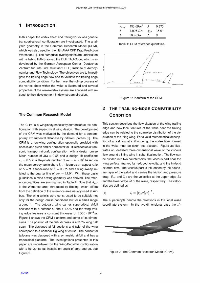
The CRM is a wing/body/nacelle/pylon/horizontal-tail con-figuration with supercritical wing design. The developmentof the CRM was motivated by the demand for a contem-porary experimental database by different parties [2]. TheCRM is a low-wing configuration optionally provided withnacelle and pylon and/or horizontal tail. It is based on a tran-sonic transport-aircraft configuration with a design cruiseMach number of Ma = 0.85 and a design lift coefficientcL = 0.5 at a Reynolds number of Re = 40 · 106 based onthe mean aerodynamic chord lµ . It features an aspect-ratioof Λ = 9, a taper-ratio of λ = 0.275 and a wing sweep re-lated to the quarter line of ϕ25 = 35.0 . With these basicguidelines in mind a wing geometry was derived. The refer-ence quantities are summarised in Table 1. Note that Are f

is the Wimpress area introduced by Boeing, which differsfrom the definition of the reference area usually used at Air-bus. The wing airfoils were constructed to be suitable notonly for the design cruise conditions but for a small rangearound it. The outboard wing carries supercritical airfoilsections with a camber of about 1.5 % and the wing trail-ing edge features a constant thickness of 3.556 · 10−4 m.Figure 1 shows the CRM planform and some of its dimen-sions. The position of the Yehudi break is at 37 % wing halfspan. The designed airfoil sections and twist of the wingcorrespond to a nominal 1-g wing at cruise. The horizontaltailplane was designed with a symmetric airfoil and has atrapezoidal planform. The investigations presented in thispaper are undertaken on the Wing/Body/Tail configurationwith a horizontal-tail installation angle of zero degree, seeFigure 2.

Are f 383.69m2 λ 0.275lµ 7.00532m ϕ25 35.0

b 58.763m Λ 9

Table 1: CRM reference quantities.

Figure 1: Planform of the CRM.

2 THE TRAILING-EDGE COMPATIBILITY

CONDITION

This section describes the flow situation at the wing trailingedge and how local features of the wake near the trailingedge can be related to the spanwise distribution of the cir-culation at the lfting wing. For a valid mathematical descrip-tion of a real flow at a lifting wing, the vortex layer formedin the wake must be taken into account. Figure 3a illus-trates an idealised three-dimensional wake of the viscousflow around a lifting wing in subcritical motion. The flow canbe divided into two counterparts, the viscous part near thewing surface, marked by reduced velocity, and the inviscidexternal flow. The viscous part is influenced by the bound-ary layer of the airfoil and carries the friction and pressuredrag. ~ve,u and ~ve,l are the velocities at the upper edge δuand the lower edge δ l of the wake, respectively. The veloc-ities are defined as

(1) ~ve =[v1

e ,v2e ,v

3e]T

.

The superscripts denote the directions in the local wakecoordinate system. In the two-dimensional case the x1-

Figure 2: The Common Research Model (CRM).

Deutscher Luft- und Raumfahrtkongress 2016

2©2016

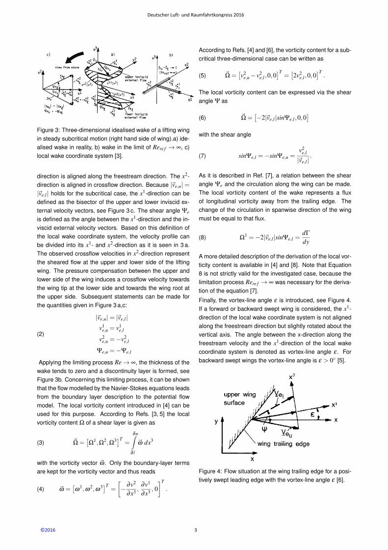
Figure 3: Three-dimensional idealised wake of a lifting wingin steady subcritical motion (right hand side of wing).a) ide-alised wake in reality, b) wake in the limit of Rere f → ∞, c)local wake coordinate system [3].

direction is aligned along the freestream direction. The x2-direction is aligned in crossflow direction. Because |~ve,u|=|~ve,l | holds for the subcritical case, the x1-direction can bedefined as the bisector of the upper and lower inviscid ex-ternal velocity vectors, see Figure 3 c. The shear angle Ψe

is defined as the angle between the x1-direction and the in-viscid external velocity vectors. Based on this definition ofthe local wake coordinate system, the velocity profile canbe divided into its x1- and x2-direction as it is seen in 3 a.The observed crossflow velocities in x2-direction representthe sheared flow at the upper and lower side of the liftingwing. The pressure compensation between the upper andlower side of the wing induces a crossflow velocity towardsthe wing tip at the lower side and towards the wing root atthe upper side. Subsequent statements can be made forthe quantities given in Figure 3 a,c:

(2)

|~ve,u|= |~ve,l |v1

e,u = v1e,l

v2e,u =−v2

e,l

Ψe,u =−Ψe,l

Applying the limiting process Re→ ∞, the thickness of thewake tends to zero and a discontinuity layer is formed, seeFigure 3b. Concerning this limiting process, it can be shownthat the flow modelled by the Navier-Stokes equations leadsfrom the boundary layer description to the potential flowmodel. The local vorticity content introduced in [4] can beused for this purpose. According to Refs. [3, 5] the localvorticity content Ω of a shear layer is given as

(3) ~Ω =[Ω

1,Ω2,Ω3]T =

δu∫δ l

~ω dx3

with the vorticity vector ~ω . Only the boundary-layer termsare kept for the vorticity vector and thus reads

(4) ~ω =[ω

1,ω2,ω3]T =

[−∂v2

∂x3 ,∂v1

∂x3 , 0]T

.

According to Refs. [4] and [6], the vorticity content for a sub-critical three-dimensional case can be written as

(5) ~Ω =[v2

e,u− v2e,l ,0,0

]T=[2v2

e,l ,0,0]T

.

The local vorticity content can be expressed via the shearangle Ψ as

(6) ~Ω =[−2|~ve,l |sinΨe,l ,0,0

]with the shear angle

(7) sinΨe,l =−sinΨe,u =v2

e,l

|~ve,l |.

As it is described in Ref. [7], a relation between the shearangle Ψe and the circulation along the wing can be made.The local vorticity content of the wake represents a fluxof longitudinal vorticity away from the trailing edge. Thechange of the circulation in spanwise direction of the wingmust be equal to that flux.

(8) Ω1 =−2|~ve,l |sinΨe,l =

dΓ

dy

A more detailed description of the derivation of the local vor-ticity content is available in [4] and [8]. Note that Equation8 is not strictly valid for the investigated case, because thelimitation process Rere f → ∞ was necessary for the deriva-tion of the equation [7].

Finally, the vortex-line angle ε is introduced, see Figure 4.If a forward or backward swept wing is considered, the x1-direction of the local wake coordinate system is not alignedalong the freestream direction but slightly rotated about thevertical axis. The angle between the x-direction along thefreestream velocity and the x1-direction of the local wakecoordinate system is denoted as vortex-line angle ε . Forbackward swept wings the vortex-line angle is ε > 0 [5].

Figure 4: Flow situation at the wing trailing edge for a posi-tively swept leading edge with the vortex-line angle ε [6].


3©2016

3 NUMERICAL APPROACH

3.1 Grid Generation

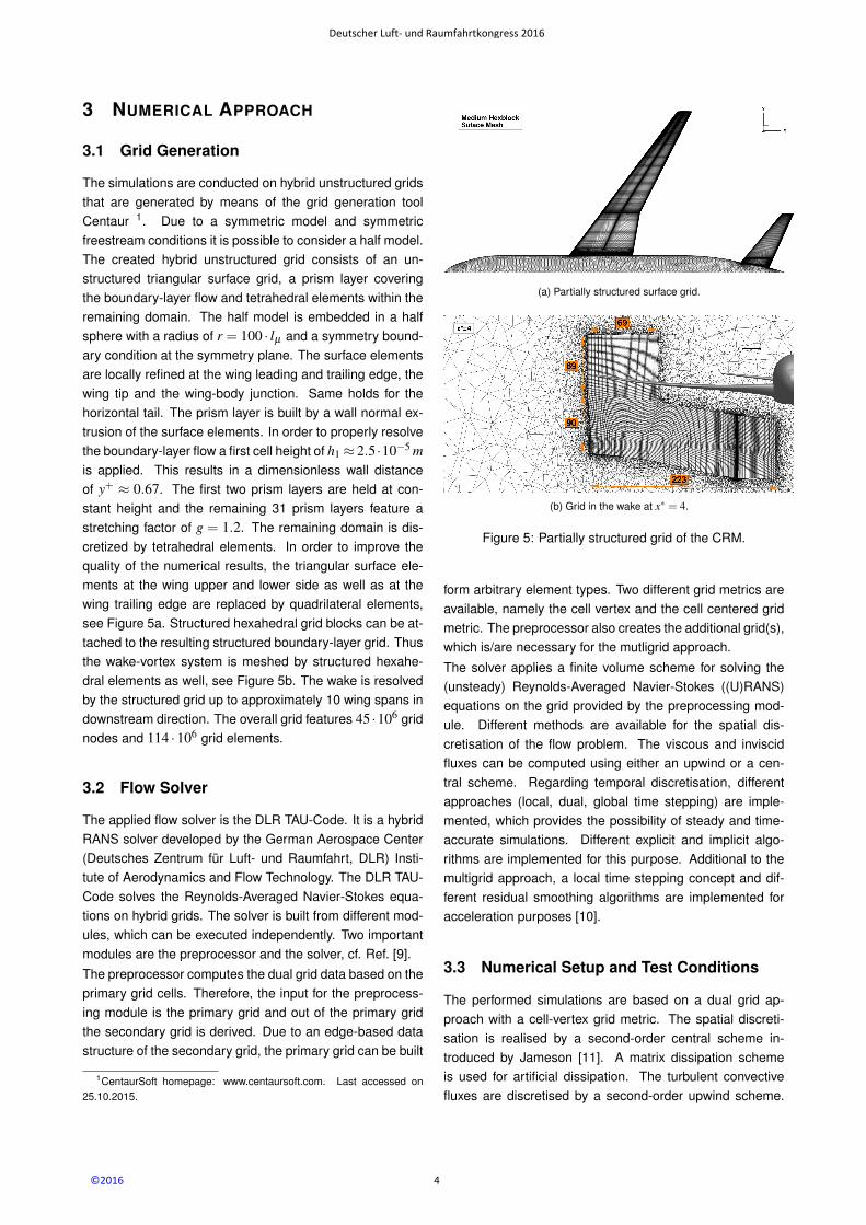
The simulations are conducted on hybrid unstructured gridsthat are generated by means of the grid generation toolCentaur 1. Due to a symmetric model and symmetricfreestream conditions it is possible to consider a half model.The created hybrid unstructured grid consists of an un-structured triangular surface grid, a prism layer coveringthe boundary-layer flow and tetrahedral elements within theremaining domain. The half model is embedded in a halfsphere with a radius of r = 100 · lµ and a symmetry bound-ary condition at the symmetry plane. The surface elementsare locally refined at the wing leading and trailing edge, thewing tip and the wing-body junction. Same holds for thehorizontal tail. The prism layer is built by a wall normal ex-trusion of the surface elements. In order to properly resolvethe boundary-layer flow a first cell height of h1≈ 2.5 ·10−5 mis applied. This results in a dimensionless wall distanceof y+ ≈ 0.67. The first two prism layers are held at con-stant height and the remaining 31 prism layers feature astretching factor of g = 1.2. The remaining domain is dis-cretized by tetrahedral elements. In order to improve thequality of the numerical results, the triangular surface ele-ments at the wing upper and lower side as well as at thewing trailing edge are replaced by quadrilateral elements,see Figure 5a. Structured hexahedral grid blocks can be at-tached to the resulting structured boundary-layer grid. Thusthe wake-vortex system is meshed by structured hexahe-dral elements as well, see Figure 5b. The wake is resolvedby the structured grid up to approximately 10 wing spans indownstream direction. The overall grid features 45 ·106 gridnodes and 114 ·106 grid elements.

3.2 Flow Solver

The applied flow solver is the DLR TAU-Code. It is a hybridRANS solver developed by the German Aerospace Center(Deutsches Zentrum fur Luft- und Raumfahrt, DLR) Insti-tute of Aerodynamics and Flow Technology. The DLR TAU-Code solves the Reynolds-Averaged Navier-Stokes equa-tions on hybrid grids. The solver is built from different mod-ules, which can be executed independently. Two importantmodules are the preprocessor and the solver, cf. Ref. [9].The preprocessor computes the dual grid data based on theprimary grid cells. Therefore, the input for the preprocess-ing module is the primary grid and out of the primary gridthe secondary grid is derived. Due to an edge-based datastructure of the secondary grid, the primary grid can be built

1CentaurSoft homepage: www.centaursoft.com. Last accessed on25.10.2015.

(a) Partially structured surface grid.

(b) Grid in the wake at x∗ = 4.

Figure 5: Partially structured grid of the CRM.

form arbitrary element types. Two different grid metrics areavailable, namely the cell vertex and the cell centered gridmetric. The preprocessor also creates the additional grid(s),which is/are necessary for the mutligrid approach.

The solver applies a finite volume scheme for solving the(unsteady) Reynolds-Averaged Navier-Stokes ((U)RANS)equations on the grid provided by the preprocessing mod-ule. Different methods are available for the spatial dis-cretisation of the flow problem. The viscous and inviscidfluxes can be computed using either an upwind or a cen-tral scheme. Regarding temporal discretisation, differentapproaches (local, dual, global time stepping) are imple-mented, which provides the possibility of steady and time-accurate simulations. Different explicit and implicit algo-rithms are implemented for this purpose. Additional to themultigrid approach, a local time stepping concept and dif-ferent residual smoothing algorithms are implemented foracceleration purposes [10].

3.3 Numerical Setup and Test Conditions

The performed simulations are based on a dual grid ap-proach with a cell-vertex grid metric. The spatial discreti-sation is realised by a second-order central scheme in-troduced by Jameson [11]. A matrix dissipation schemeis used for artificial dissipation. The turbulent convectivefluxes are discretised by a second-order upwind scheme.


4©2016

The temporal discretisation is done by an implicit Backward-Euler scheme. The applied version uses a LU-SGS al-gorithm [12]. The unsteady simulations using the dualtime approach are performed with a physical timestep of∆t = 4.6 · 10−4 s. 150 inner iterations are conducted foreach timestep. In order to accelerate the convergence ofthe solution, a 3v-multigrid cycle is used [13]. Turbulencemodeling is realised by means of the Menter-SST eddy-viscosity turbulence model. The Schwarz limitation andthe Positivity scheme are applied to increase stability [14].The analysis is performed for one target flow condition witha Mach number of Ma∞ = 0.85, a Reynolds number ofRe = 5 · 106, based on the mean aerodynamic chord lµ ,and an angle of attack of α = 2. The reference tem-perature of T∞ = 310.93K results in a freestream velocityof U∞ = 300.48m/s. The Reynolds number is chosen inaccordance with former experimental investigations at theNASA Langley National Transonic Facility by Rivers andDittberner [15]. The experimental results are used in orderto evaluate the numerical results by means of surface pres-sure distributions, cf. Ref. [16]. The resulting flight conditionfeatures a lift coefficient of cL = 0.43.

4 RESULTS AND DISCUSSION

4.1 Flow Past the Wing

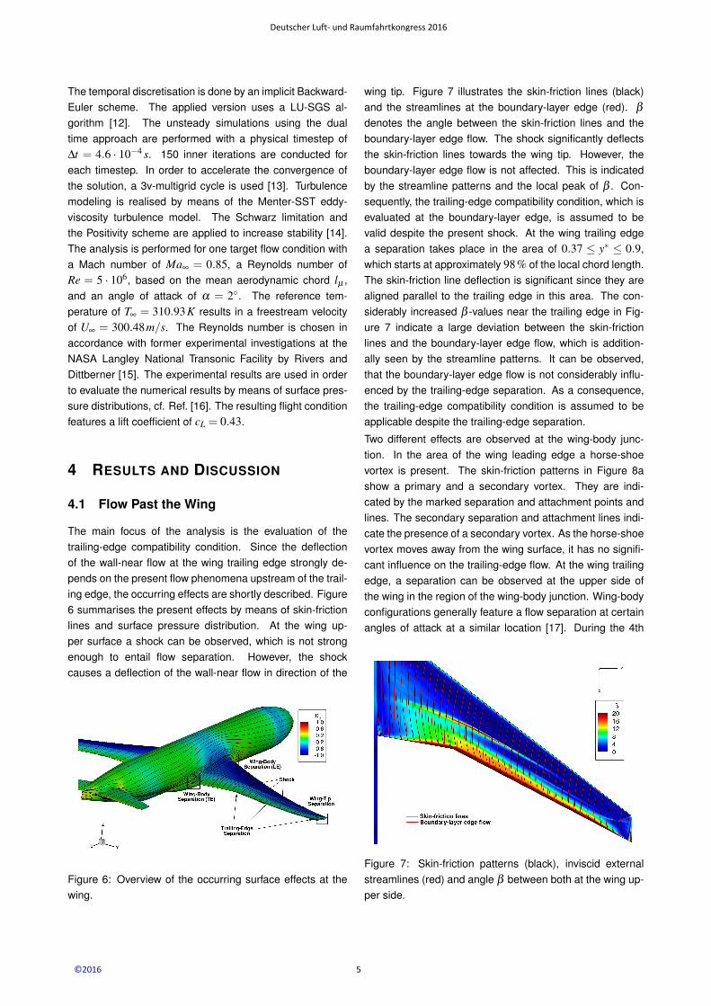
The main focus of the analysis is the evaluation of thetrailing-edge compatibility condition. Since the deflectionof the wall-near flow at the wing trailing edge strongly de-pends on the present flow phenomena upstream of the trail-ing edge, the occurring effects are shortly described. Figure6 summarises the present effects by means of skin-frictionlines and surface pressure distribution. At the wing up-per surface a shock can be observed, which is not strongenough to entail flow separation. However, the shockcauses a deflection of the wall-near flow in direction of the

Figure 6: Overview of the occurring surface effects at thewing.

wing tip. Figure 7 illustrates the skin-friction lines (black)and the streamlines at the boundary-layer edge (red). β

denotes the angle between the skin-friction lines and theboundary-layer edge flow. The shock significantly deflectsthe skin-friction lines towards the wing tip. However, theboundary-layer edge flow is not affected. This is indicatedby the streamline patterns and the local peak of β . Con-sequently, the trailing-edge compatibility condition, which isevaluated at the boundary-layer edge, is assumed to bevalid despite the present shock. At the wing trailing edgea separation takes place in the area of 0.37 ≤ y∗ ≤ 0.9,which starts at approximately 98% of the local chord length.The skin-friction line deflection is significant since they arealigned parallel to the trailing edge in this area. The con-siderably increased β -values near the trailing edge in Fig-ure 7 indicate a large deviation between the skin-frictionlines and the boundary-layer edge flow, which is addition-ally seen by the streamline patterns. It can be observed,that the boundary-layer edge flow is not considerably influ-enced by the trailing-edge separation. As a consequence,the trailing-edge compatibility condition is assumed to beapplicable despite the trailing-edge separation.

Two different effects are observed at the wing-body junc-tion. In the area of the wing leading edge a horse-shoevortex is present. The skin-friction patterns in Figure 8ashow a primary and a secondary vortex. They are indi-cated by the marked separation and attachment points andlines. The secondary separation and attachment lines indi-cate the presence of a secondary vortex. As the horse-shoevortex moves away from the wing surface, it has no signifi-cant influence on the trailing-edge flow. At the wing trailingedge, a separation can be observed at the upper side ofthe wing in the region of the wing-body junction. Wing-bodyconfigurations generally feature a flow separation at certainangles of attack at a similar location [17]. During the 4th

Figure 7: Skin-friction patterns (black), inviscid externalstreamlines (red) and angle β between both at the wing up-per side.


5©2016

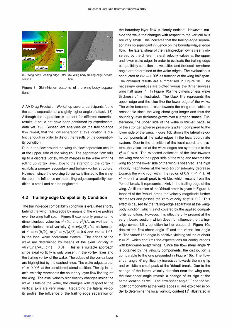
(a) Wing-body leading-edge inter-section.

(b) Wing-body trailing-edge separa-tion.

Figure 8: Skin-friction patterns of the wing-body separa-tions.

AIAA Drag Prediction Workshop several participants foundthe same separation at a slightly higher angle of attack [18].Although the separation is present for different numericalresults, it could not have been confirmed by experimentaldata yet [19]. Subsequent analyses on the trailing-edgeflow reveal, that the flow separation at this location is dis-tinct enough in order to distort the results of the compatibil-ity condition.

Due to the flow around the wing tip, flow separation occursat the upper side of the wing tip. The separated flow rollsup to a discrete vortex, which merges in the wake with therolling up vortex layer. Due to the strength of the vortex itexhibits a primary, secondary and tertiary vortex structure.However, since the evolving tip vortex is limited to the wing-tip area, the influence on the trailing-edge compatibility con-dition is small and can be neglected.

4.2 Trailing-Edge Compatibility Condition

The trailing-edge compatibility condition is evaluated shortlybehind the wing trailing edge by means of the wake profilesover the wing half span. Figure 9 exemplarily presents thedimensionless velocities v1/U∞ and v2/U∞ as well as thedimensionless axial vorticity ζ = ω(b/2)/U∞ as functionof z∗ = z/(b/2), at y∗ = y/(b/2) = 0.6 and x/c = 1.03,in the local wake coordinate system. The edges of thewake are determined by means of the axial vorticity atω(y∗,z∗)/ωmax(y∗) = 0.01. This is a suitable approachsince axial vorticity is only present in the vortex layer andthe trailing vortex of the wake. The edges of the vortex layerare highlighted by the dashed lines. The wake edges are atz∗≈ |0.005| at the considered lateral position. The dip in theaxial velocity represents the boundary-layer flow floating-offthe wing. The axial velocity significantly changes inside thewake. Outside the wake, the changes with respect to thevertical axis are very small. Regarding the lateral veloc-ity profile, the influence of the trailing-edge separation on

the boundary-layer flow is clearly noticed. However, out-side the wake the changes with respect to the vertical axisare very small. This indicates that the trailing-edge separa-tion has no significant influence on the boundary-layer edgeflow. The lateral shear of the trailing-edge flow is clearly ob-served by the different lateral velocity values at the upperand lower wake edge. In order to evaluate the trailing-edgecompatibility condition the velocities and the local flow shearangle are determined at the wake edges. The evaluation isconducted at x/c = 1.005 as function of the wing half span.The obtained results are summarised in Figure 10. Thenecessary quantities are plotted versus the dimensionlesswing half span y∗. In Figure 10a the dimensionless wakethickness z∗ is illustrated. The black line represents theupper edge and the blue line the lower edge of the wake.The wake becomes thicker towards the wing root, which isreasonable since the wing chord gets longer and thus theboundary-layer thickness grows over a larger distance. Fur-thermore, the upper side of the wake is thicker, becauseof the stronger adverse pressure gradient compared to thelower side of the wing. Figure 10b shows the lateral veloc-ity components at the wake edges in the local coordinatesystem. Due to the definition of the local coordinate sys-tem, the velocities at the wake edges are symmetric to thev2

e = 0 axis. The expected deflection of the flow towardsthe wing root on the upper side of the wing and towards thewing tip on the lower side of the wing is observed. The highvelocity magnitudes at the wing tip considerably decreasetowards the wing root within the region of 0.8 ≤ y∗ ≤ 1. Aty∗ = 0.37 a small peak is visible, which results from theYehudi break. It represents a kink in the trailing edge of thewing. An illustration of the Yehudi break is given in Figure 1.Inboard of the Yehudi break the velocity magnitude furtherdecreases and passes the zero velocity at y∗ ≈ 0.2. Thiseffect is caused by the trailing-edge separation at the wing-body junction, which is not covered by the applied compat-ibility condition. However, this effect is only present at thevery inboard section, which does not influence the trailing-edge compatibility condition further outboard. Figure 10cdepicts the flow-shear angle Ψ and the vortex-line angleε . The vortex-line angle is positive yielding values of aboutε ≈ 2, which confirms the expectations for configurationswith backward-swept wings. Since the flow-shear angle Ψ

is obtained by the velocity components, the distribution iscomparable to the one presented in Figure 10b. The flow-shear angle Ψ significantly increases towards the wing tipand exhibits a small peak at the Yehudi break. Due to thechange of the lateral velocity direction near the wing root,the flow-shear angle reveals a change of its sign at thesame location as well. The flow-shear angle Ψ and the ve-locity components at the wake edges ve are exploited in or-der to determine the local vorticity content Ω1, illustrated in


6©2016

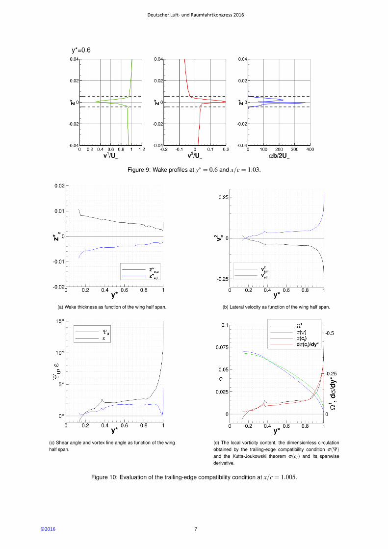
Figure 9: Wake profiles at y∗ = 0.6 and x/c = 1.03.

(a) Wake thickness as function of the wing half span. (b) Lateral velocity as function of the wing half span.

(c) Shear angle and vortex line angle as function of the winghalf span.

(d) The local vorticity content, the dimensionless circulationobtained by the trailing-edge compatibility condition σ(Ψ)

and the Kutta-Joukowski theorem σ(cl) and its spanwisederivative.

Figure 10: Evaluation of the trailing-edge compatibility condition at x/c = 1.005.


7©2016

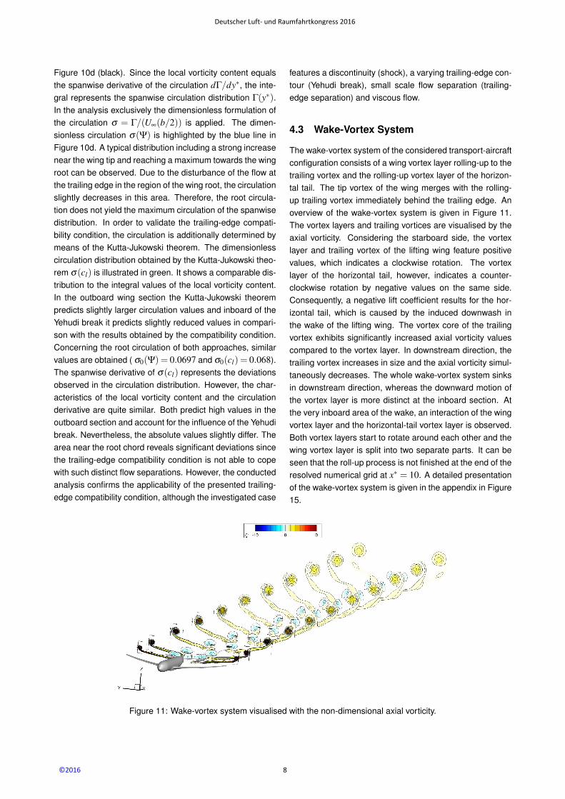
Figure 10d (black). Since the local vorticity content equalsthe spanwise derivative of the circulation dΓ/dy∗, the inte-gral represents the spanwise circulation distribution Γ(y∗).In the analysis exclusively the dimensionless formulation ofthe circulation σ = Γ/(U∞(b/2)) is applied. The dimen-sionless circulation σ(Ψ) is highlighted by the blue line inFigure 10d. A typical distribution including a strong increasenear the wing tip and reaching a maximum towards the wingroot can be observed. Due to the disturbance of the flow atthe trailing edge in the region of the wing root, the circulationslightly decreases in this area. Therefore, the root circula-tion does not yield the maximum circulation of the spanwisedistribution. In order to validate the trailing-edge compati-bility condition, the circulation is additionally determined bymeans of the Kutta-Jukowski theorem. The dimensionlesscirculation distribution obtained by the Kutta-Jukowski theo-rem σ(cl) is illustrated in green. It shows a comparable dis-tribution to the integral values of the local vorticity content.In the outboard wing section the Kutta-Jukowski theorempredicts slightly larger circulation values and inboard of theYehudi break it predicts slightly reduced values in compari-son with the results obtained by the compatibility condition.Concerning the root circulation of both approaches, similarvalues are obtained ( σ0(Ψ) = 0.0697 and σ0(cl) = 0.068).The spanwise derivative of σ(cl) represents the deviationsobserved in the circulation distribution. However, the char-acteristics of the local vorticity content and the circulationderivative are quite similar. Both predict high values in theoutboard section and account for the influence of the Yehudibreak. Nevertheless, the absolute values slightly differ. Thearea near the root chord reveals significant deviations sincethe trailing-edge compatibility condition is not able to copewith such distinct flow separations. However, the conductedanalysis confirms the applicability of the presented trailing-edge compatibility condition, although the investigated case

features a discontinuity (shock), a varying trailing-edge con-tour (Yehudi break), small scale flow separation (trailing-edge separation) and viscous flow.

4.3 Wake-Vortex System

The wake-vortex system of the considered transport-aircraftconfiguration consists of a wing vortex layer rolling-up to thetrailing vortex and the rolling-up vortex layer of the horizon-tal tail. The tip vortex of the wing merges with the rolling-up trailing vortex immediately behind the trailing edge. Anoverview of the wake-vortex system is given in Figure 11.The vortex layers and trailing vortices are visualised by theaxial vorticity. Considering the starboard side, the vortexlayer and trailing vortex of the lifting wing feature positivevalues, which indicates a clockwise rotation. The vortexlayer of the horizontal tail, however, indicates a counter-clockwise rotation by negative values on the same side.Consequently, a negative lift coefficient results for the hor-izontal tail, which is caused by the induced downwash inthe wake of the lifting wing. The vortex core of the trailingvortex exhibits significantly increased axial vorticity valuescompared to the vortex layer. In downstream direction, thetrailing vortex increases in size and the axial vorticity simul-taneously decreases. The whole wake-vortex system sinksin downstream direction, whereas the downward motion ofthe vortex layer is more distinct at the inboard section. Atthe very inboard area of the wake, an interaction of the wingvortex layer and the horizontal-tail vortex layer is observed.Both vortex layers start to rotate around each other and thewing vortex layer is split into two separate parts. It can beseen that the roll-up process is not finished at the end of theresolved numerical grid at x∗ = 10. A detailed presentationof the wake-vortex system is given in the appendix in Figure15.

Figure 11: Wake-vortex system visualised with the non-dimensional axial vorticity.


8©2016

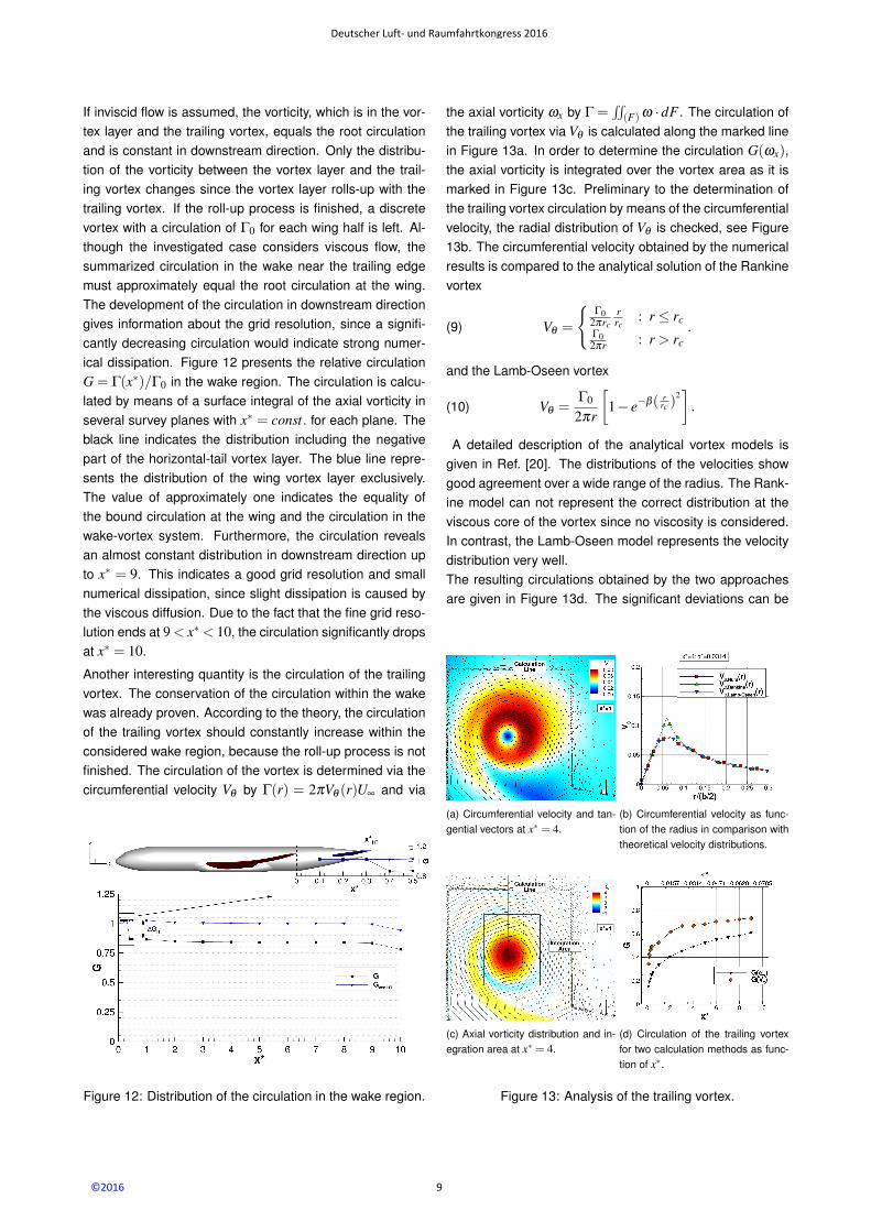
If inviscid flow is assumed, the vorticity, which is in the vor-tex layer and the trailing vortex, equals the root circulationand is constant in downstream direction. Only the distribu-tion of the vorticity between the vortex layer and the trail-ing vortex changes since the vortex layer rolls-up with thetrailing vortex. If the roll-up process is finished, a discretevortex with a circulation of Γ0 for each wing half is left. Al-though the investigated case considers viscous flow, thesummarized circulation in the wake near the trailing edgemust approximately equal the root circulation at the wing.The development of the circulation in downstream directiongives information about the grid resolution, since a signifi-cantly decreasing circulation would indicate strong numer-ical dissipation. Figure 12 presents the relative circulationG = Γ(x∗)/Γ0 in the wake region. The circulation is calcu-lated by means of a surface integral of the axial vorticity inseveral survey planes with x∗ = const. for each plane. Theblack line indicates the distribution including the negativepart of the horizontal-tail vortex layer. The blue line repre-sents the distribution of the wing vortex layer exclusively.The value of approximately one indicates the equality ofthe bound circulation at the wing and the circulation in thewake-vortex system. Furthermore, the circulation revealsan almost constant distribution in downstream direction upto x∗ = 9. This indicates a good grid resolution and smallnumerical dissipation, since slight dissipation is caused bythe viscous diffusion. Due to the fact that the fine grid reso-lution ends at 9< x∗ < 10, the circulation significantly dropsat x∗ = 10.

Another interesting quantity is the circulation of the trailingvortex. The conservation of the circulation within the wakewas already proven. According to the theory, the circulationof the trailing vortex should constantly increase within theconsidered wake region, because the roll-up process is notfinished. The circulation of the vortex is determined via thecircumferential velocity Vθ by Γ(r) = 2πVθ (r)U∞ and via

Figure 12: Distribution of the circulation in the wake region.

the axial vorticity ωx by Γ =∫∫

(F) ω ·dF . The circulation ofthe trailing vortex via Vθ is calculated along the marked linein Figure 13a. In order to determine the circulation G(ωx),the axial vorticity is integrated over the vortex area as it ismarked in Figure 13c. Preliminary to the determination ofthe trailing vortex circulation by means of the circumferentialvelocity, the radial distribution of Vθ is checked, see Figure13b. The circumferential velocity obtained by the numericalresults is compared to the analytical solution of the Rankinevortex

(9) Vθ =

Γ0

2πrcrrc

: r ≤ rcΓ02πr : r > rc

.

and the Lamb-Oseen vortex

(10) Vθ =Γ0

2πr

[1− e−β( r

rc )2].

A detailed description of the analytical vortex models isgiven in Ref. [20]. The distributions of the velocities showgood agreement over a wide range of the radius. The Rank-ine model can not represent the correct distribution at theviscous core of the vortex since no viscosity is considered.In contrast, the Lamb-Oseen model represents the velocitydistribution very well.The resulting circulations obtained by the two approachesare given in Figure 13d. The significant deviations can be

(a) Circumferential velocity and tan-gential vectors at x∗ = 4.

(b) Circumferential velocity as func-tion of the radius in comparison withtheoretical velocity distributions.

(c) Axial vorticity distribution and in-egration area at x∗ = 4.

(d) Circulation of the trailing vortexfor two calculation methods as func-tion of x∗.

Figure 13: Analysis of the trailing vortex.


9©2016

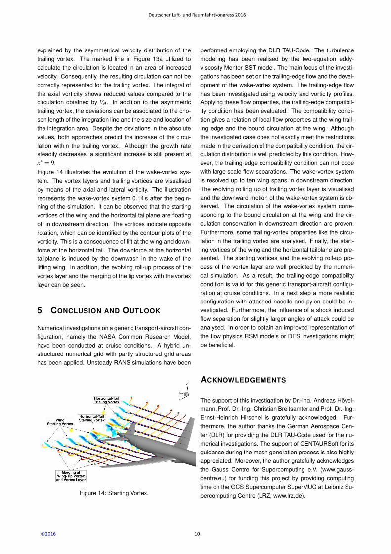
explained by the asymmetrical velocity distribution of thetrailing vortex. The marked line in Figure 13a utilized tocalculate the circulation is located in an area of increasedvelocity. Consequently, the resulting circulation can not becorrectly represented for the trailing vortex. The integral ofthe axial vorticity shows reduced values compared to thecirculation obtained by Vθ . In addition to the asymmetrictrailing vortex, the deviations can be associated to the cho-sen length of the integration line and the size and location ofthe integration area. Despite the deviations in the absolutevalues, both approaches predict the increase of the circu-lation within the trailing vortex. Although the growth ratesteadily decreases, a significant increase is still present atx∗ = 9.

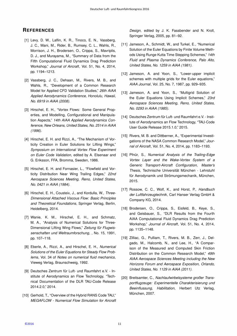
Figure 14 illustrates the evolution of the wake-vortex sys-tem. The vortex layers and trailing vortices are visualisedby means of the axial and lateral vorticity. The illustrationrepresents the wake-vortex system 0.14 s after the begin-ning of the simulation. It can be observed that the startingvortices of the wing and the horizontal tailplane are floatingoff in downstream direction. The vortices indicate oppositerotation, which can be identified by the contour plots of thevorticity. This is a consequence of lift at the wing and down-force at the horizontal tail. The downforce at the horizontaltailplane is induced by the downwash in the wake of thelifting wing. In addition, the evolving roll-up process of thevortex layer and the merging of the tip vortex with the vortexlayer can be seen.

5 CONCLUSION AND OUTLOOK

Numerical investigations on a generic transport-aircraft con-figuration, namely the NASA Common Research Model,have been conducted at cruise conditions. A hybrid un-structured numerical grid with partly structured grid areashas been applied. Unsteady RANS simulations have been

Figure 14: Starting Vortex.

performed employing the DLR TAU-Code. The turbulencemodelling has been realised by the two-equation eddy-viscosity Menter-SST model. The main focus of the investi-gations has been set on the trailing-edge flow and the devel-opment of the wake-vortex system. The trailing-edge flowhas been investigated using velocity and vorticity profiles.Applying these flow properties, the trailing-edge compatibil-ity condition has been evaluated. The compatibility condi-tion gives a relation of local flow properties at the wing trail-ing edge and the bound circulation at the wing. Althoughthe investigated case does not exactly meet the restrictionsmade in the derivation of the compatibility condition, the cir-culation distribution is well predicted by this condition. How-ever, the trailing-edge compatibility condition can not copewith large scale flow separations. The wake-vortex systemis resolved up to ten wing spans in downstream direction.The evolving rolling up of trailing vortex layer is visualisedand the downward motion of the wake-vortex system is ob-served. The circulation of the wake-vortex system corre-sponding to the bound circulation at the wing and the cir-culation conservation in downstream direction are proven.Furthermore, some trailing-vortex properties like the circu-lation in the trailing vortex are analysed. Finally, the start-ing vortices of the wing and the horizontal tailplane are pre-sented. The starting vortices and the evolving roll-up pro-cess of the vortex layer are well predicted by the numeri-cal simulation. As a result, the trailing-edge compatibilitycondition is valid for this generic transport-aircraft configu-ration at cruise conditions. In a next step a more realisticconfiguration with attached nacelle and pylon could be in-vestigated. Furthermore, the influence of a shock inducedflow separation for slightly larger angles of attack could beanalysed. In order to obtain an improved representation ofthe flow physics RSM models or DES investigations mightbe beneficial.

ACKNOWLEDGEMENTS

The support of this investigation by Dr.-Ing. Andreas Hovel-mann, Prof. Dr.-Ing. Christian Breitsamter and Prof. Dr.-Ing.Ernst-Heinrich Hirschel is gratefully acknowledged. Fur-thermore, the author thanks the German Aerospace Cen-ter (DLR) for providing the DLR TAU-Code used for the nu-merical investigations. The support of CENTAURSoft for itsguidance during the mesh generation process is also highlyappreciated. Moreover, the author gratefully acknowledgesthe Gauss Centre for Supercomputing e.V. (www.gauss-centre.eu) for funding this project by providing computingtime on the GCS Supercomputer SuperMUC at Leibniz Su-percomputing Centre (LRZ, www.lrz.de).


10©2016

REFERENCES

[1] Levy, D. W., Laflin, K. R., Tinoco, E. N., Vassberg,J. C., Mani, M., Rider, B., Rumsey, C. L., Wahls, R.,Morrison, J. H., Brodersen, O., Crippa, S., Mavriplis,D. J., and Murayama, M., “Summary of Data from theFifth Computational Fluid Dynamics Drag PredictionWorkshop,” Journal of Aircraft , Vol. 51, No. 4, 2014,pp. 1194–1213.

[2] Vassberg, J. C., Dehaan, M., Rivers, M. B., andWahls, R., “Development of a Common ResearchModel for Applied CFD Validation Studies,” 26th AIAAApplied Aerodynamics Conference, Honolulu, Hawaii,No. 6919 in AIAA (2008).

[3] Hirschel, E. H., “Vortex Flows: Some General Prop-erties, and Modelling, Configurational and Manipula-tion Aspects,” 14th AIAA Applied Aerodynamics Con-ference, New Orleans, United States, No. 2514 in AIAA(1996).

[4] Hirschel, E. H. and Rizzi, A., “The Mechanism of Vor-ticity Creation in Euler Solutions for Lifting Wings,”Symposium on International Vortex Flow Experimenton Euler Code Validation, edited by A. Elsenaar andG. Eriksson, FFA, Bromma, Sweden, 1986.

[5] Hirschel, E. H. and Fornasier, L., “Flowfield and Vor-ticity Distribution Near Wing Trailing Edges,” 22ndAerospace Sciences Meeting, Reno, United States,No. 0421 in AIAA (1984).

[6] Hirschel, E. H., Cousteix, J., and Kordulla, W., Three-Dimensional Attached Viscous Flow: Basic Principlesand Theoretical Foundations, Springer Verlag, Berlin,Heidelberg, 2014.

[7] Wanie, K. M., Hirschel, E. H., and Schmatz,M. A., “Analysis of Numerical Solutions for Three-Dimensional Lifting Wing Flows,” Zeitung fur Flugwis-senschaften und Weltraumforschung, , No. 15, 1991,pp. 107–118.

[8] Eberle, A., Rizzi, A., and Hirschel, E. H., NumericalSolutions of the Euler Equations for Steady Flow Prob-lems, Vol. 34 of Notes on numerical fluid mechanics,Vieweg Verlag, Braunschweig, 1992.

[9] Deutsches Zentrum fur Luft- und Raumfahrt e.V. - In-stitute of Aerodynamics an Flow Technology, “Tech-nical Documentation of the DLR TAU-Code Release2014.2.0,” 2014.

[10] Gerhold, T., “Overview of the Hybrid RANS Code TAU,”MEGAFLOW - Numerical Flow Simulation for Aircraft

Design, edited by J. K. Fassbender and N. Kroll,Springer Verlag, 2005, pp. 81–92.

[11] Jameson, A., Schmidt, W., and Turkel, E., “NumericalSolution of the Euler Equations by Finite Volume Meth-ods Using Runge Kutta Time Stepping Schemes,” 14thFluid and Plasma Dynamics Conference, Palo Alto,United States, No. 1259 in AIAA (1981).

[12] Jameson, A. and Yoon, S., “Lower-upper implicitschemes with multiple grids for the Euler equations,”AIAA Journal , Vol. 25, No. 7, 1987, pp. 929–935.

[13] Jameson, A. and Yoon, S., “Multigrid Solution ofthe Euler Equations Using Implicit Schemes,” 23rdAerospace Sciences Meeting, Reno, United States,No. 0293 in AIAA (1985).

[14] Deutsches Zentrum fur Luft- und Raumfahrt e.V. - Insti-tute of Aerodynamics an Flow Technology, “TAU-CodeUser Guide Release 2015.1.0,” 2015.

[15] Rivers, M. B. and Dittberner, A., “Experimental Investi-gations of the NASA Common Research Model,” Jour-nal of Aircraft , Vol. 51, No. 4, 2014, pp. 1183–1193.

[16] Pfnur, S., Numerical Analysis of the Trailing-EdgeVortex Layer and the Wake-Vortex System of aGeneric Transport-Aircraft Configuration, Master’sThesis, Technische Universitat Munchen - Lehrstuhlfur Aerodynamik und Stromungsmechanik, Munchen,2015.

[17] Rossow, C. C., Wolf, K., and Horst, P., Handbuchder Luftfahrzeugtechnik , Carl Hanser Verlag GmbH &Company KG, 2014.

[18] Brodersen, O., Crippa, S., Eisfeld, B., Keye, S.,and Geisbauer, S., “DLR Results from the FourthAIAA Computational Fluid Dynamics Drag PredictionWorkshop,” Journal of Aircraft , Vol. 51, No. 4, 2014,pp. 1135–1148.

[19] Zilliac, G., Pulliam, T., Rivers, M. B., Zerr, J., Del-gado, M., Halcomb, N., and Lee, H., “A Compar-ison of the Measured and Computed Skin FrictionDistribution on the Common Research Model,” 49thAIAA Aerospace Sciences Meeting including the NewHorizons Forum and Aerospace Exposition, Orlando,United States, No. 1129 in AIAA (2011).

[20] Breitsamter, C., Nachlaufwirbelsysteme großer Trans-portflugzeuge: Experimentelle Charakterisierung undBeeinflussung, Habilitation, Herbert Utz Verlag,Munchen, 2007.


11©2016

APPENDIX

A Wake-Vortex System

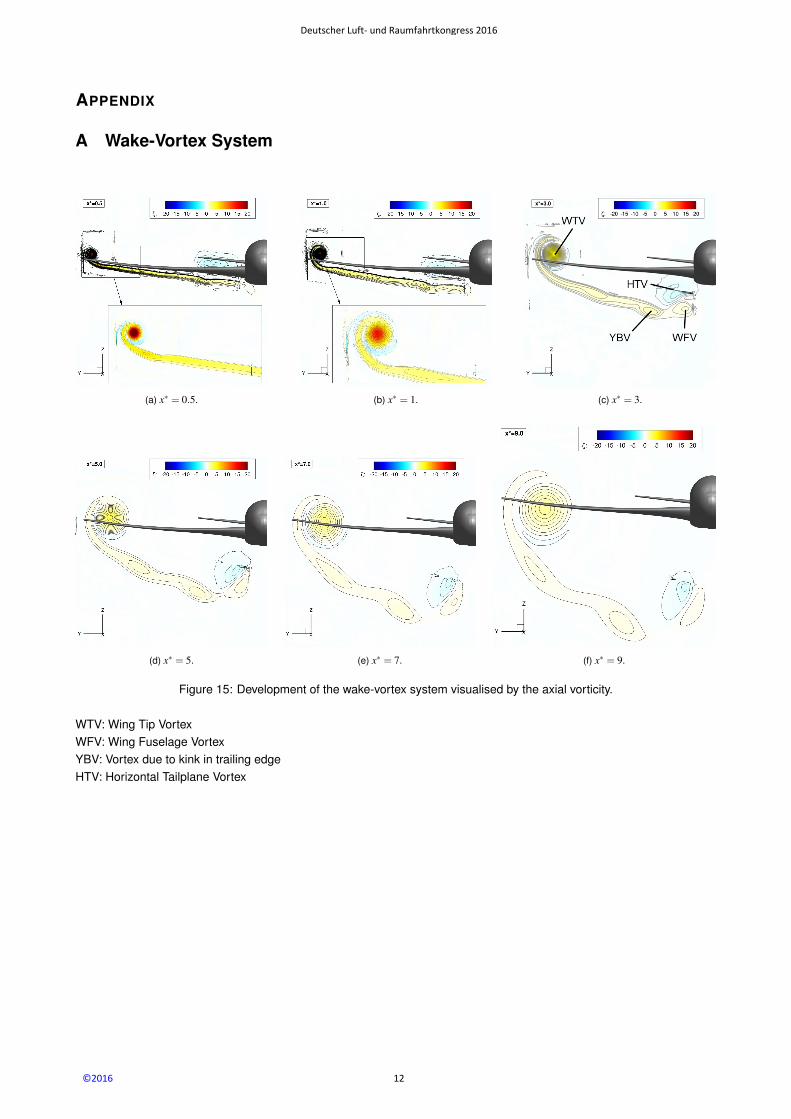
(a) x∗ = 0.5. (b) x∗ = 1. (c) x∗ = 3.

(d) x∗ = 5. (e) x∗ = 7. (f) x∗ = 9.

Figure 15: Development of the wake-vortex system visualised by the axial vorticity.

WTV: Wing Tip VortexWFV: Wing Fuselage VortexYBV: Vortex due to kink in trailing edgeHTV: Horizontal Tailplane Vortex


12©2016

Documents

NUMERICAL ANALYSIS OF THE TRAILING-EDGE VORTEX LAYER · PDF filenumerical analysis of the trailing-edge vortex layer and the wake-vortex system of a generic transport-aircraft configuration