Numerical Analysis of Power System Transients and Dynamics

IET POWER AND ENERGY SERIES 78

Numerical Analysisof Power System

Transients andDynamics

Other volumes in this series:

Volume 1 Power circuit breaker theory and design C.H. Flurscheim (Editor)Volume 4 Industrial microwave heating A.C. Metaxas and R.J. MeredithVolume 7 Insulators for high voltages J.S.T. LoomsVolume 8 Variable frequency ac motor drive systems D. FinneyVolume 10 SF6 switchgear H.M. Ryan and G.R. JonesVolume 11 Conduction and induction heating E.J. DaviesVolume 13 Statistical techniques for high voltage engineering W. Hauschild and W. MoschVolume 14 Uninterruptible power supplies J. Platts and J.D. St Aubyn (Editors)Volume 15 Digital protection for power systems A.T. Johns and S.K. SalmanVolume 16 Electricity economics and planning T.W. BerrieVolume 18 Vacuum switchgear A. GreenwoodVolume 19 Electrical safety: a guide to causes and prevention of hazards J. Maxwell AdamsVolume 21 Electricity distribution network design, 2nd edition E. Lakervi and E.J. HolmesVolume 22 Artificial intelligence techniques in power systems K. Warwick, A.O. Ekwue and

R. Aggarwal (Editors)Volume 24 Power system commissioning and maintenance practice K. HarkerVolume 25 Engineers’ handbook of industrial microwave heating R.J. MeredithVolume 26 Small electric motors H. Moczala et al.Volume 27 Ac-dc power system analysis J. Arrillaga and B.C. SmithVolume 29 High voltage direct current transmission, 2nd edition J. ArrillagaVolume 30 Flexible ac transmission systems (FACTS) Y-H. Song (Editor)Volume 31 Embedded generation N. Jenkins et al.Volume 32 High voltage engineering and testing, 2nd edition H.M. Ryan (Editor)Volume 33 Overvoltage protection of low-voltage systems, revised edition P. HasseVolume 36 Voltage quality in electrical power systems J. Schlabbach et al.Volume 37 Electrical steels for rotating machines P. BeckleyVolume 38 The electric car: development and future of battery, hybrid and fuel-cell cars

M. WestbrookVolume 39 Power systems electromagnetic transients simulation J. Arrillaga and N. WatsonVolume 40 Advances in high voltage engineering M. Haddad and D. WarneVolume 41 Electrical operation of electrostatic precipitators K. ParkerVolume 43 Thermal power plant simulation and control D. FlynnVolume 44 Economic evaluation of projects in the electricity supply industry H. KhatibVolume 45 Propulsion systems for hybrid vehicles J. MillerVolume 46 Distribution switchgear S. StewartVolume 47 Protection of electricity distribution networks, 2nd edition J. Gers and E. HolmesVolume 48 Wood pole overhead lines B. WareingVolume 49 Electric fuses, 3rd edition A. Wright and G. NewberyVolume 50 Wind power integration: connection and system operational aspects B. Fox et al.Volume 51 Short circuit currents J. SchlabbachVolume 52 Nuclear power J. WoodVolume 53 Condition assessment of high voltage insulation in power system equipment

R.E. James and Q. SuVolume 55 Local energy: distributed generation of heat and power J. WoodVolume 56 Condition monitoring of rotating electrical machines P. Tavner, L. Ran, J. Penman

and H. SeddingVolume 57 The control techniques drives and controls handbook, 2nd edition B. DruryVolume 58 Lightning protection V. Cooray (Editor)Volume 59 Ultracapacitor applications J.M. MillerVolume 62 Lightning electromagnetics V. CoorayVolume 63 Energy storage for power systems, 2nd edition A. Ter-GazarianVolume 65 Protection of electricity distribution networks, 3rd edition J. GersVolume 66 High voltage engineering testing, 3rd edition H. Ryan (Editor)Volume 67 Multicore simulation of power system transients F.M. UriateVolume 68 Distribution system analysis and automation J. GersVolume 69 The lightening flash, 2nd edition V. Cooray (Editor)Volume 70 Economic evaluation of projects in the electricity supply industry, 3rd edition

H. KhatibVolume 905 Power system protection, 4 volumes

Numerical Analysisof Power System

Transients andDynamics

Edited by Akihiro Ametani

The Institution of Engineering and Technology

Published by The Institution of Engineering and Technology, London, United Kingdom

The Institution of Engineering and Technology is registered as a Charity in England &Wales (no. 211014) and Scotland (no. SC038698).

† The Institution of Engineering and Technology 2015

First published 2015

This publication is copyright under the Berne Convention and the Universal CopyrightConvention. All rights reserved. Apart from any fair dealing for the purposes of researchor private study, or criticism or review, as permitted under the Copyright, Designs andPatents Act 1988, this publication may be reproduced, stored or transmitted, in anyform or by any means, only with the prior permission in writing of the publishers, or inthe case of reprographic reproduction in accordance with the terms of licences issuedby the Copyright Licensing Agency. Enquiries concerning reproduction outside thoseterms should be sent to the publisher at the undermentioned address:

The Institution of Engineering and TechnologyMichael Faraday HouseSix Hills Way, StevenageHerts, SG1 2AY, United Kingdom

www.theiet.org

While the authors and publisher believe that the information and guidance given in thiswork are correct, all parties must rely upon their own skill and judgement when makinguse of them. Neither the authors nor publisher assumes any liability to anyone for anyloss or damage caused by any error or omission in the work, whether such an error oromission is the result of negligence or any other cause. Any and all such liability isdisclaimed.

The moral rights of the authors to be identified as author of this work have beenasserted by him in accordance with the Copyright, Designs and Patents Act 1988.

British Library Cataloguing in Publication DataA catalogue record for this product is available from the British Library

ISBN 978-1-84919-849-3 (hardback)ISBN 978-1-84919-850-9 (PDF)

Typeset in India by MPS LimitedPrinted in the UK by CPI Group (UK) Ltd, Croydon

Contents

Preface xiii

1 Introduction of circuit theory-based approach and numericalelectromagnetic analysis 1A. Ametani1.1 Circuit theory-based approach: EMTP 1

1.1.1 Summary of the original EMTP 11.1.2 Nodal analysis 21.1.3 Equivalent resistive circuit 41.1.4 Sparse matrix 71.1.5 Frequency-dependent line model 81.1.6 Transformer 91.1.7 Three-phase synchronous machine 101.1.8 Universal machine 111.1.9 Switches 131.1.10 Surge arrester and protective gap (archorn) 161.1.11 Inclusion of nonlinear elements 181.1.12 TACS 201.1.13 MODELS (implemented in the ATP-EMTP) 221.1.14 Power system elements prepared in EMTP 241.1.15 Basic input data 24

1.2 Numerical electromagnetic analysis 361.2.1 Introduction 361.2.2 Maxwell’s equations 371.2.3 NEA method 381.2.4 Method of Moments in the time and frequency

domains 381.2.5 Finite-difference time-domain method 41

1.3 Conclusions 42References 42

2 EMTP-ATP 47M. Kizilcay and H.K. Hoidalen2.1 Introduction 472.2 Capabilities 48

2.2.1 Overview 482.2.2 Built-in electrical components 48

2.2.3 Embedded simulation modules TACS and MODELS 492.2.4 Supporting modules 502.2.5 Frequency-domain analysis 522.2.6 Power flow option – FIX SOURCE 522.2.7 Typical power system studies 53

2.3 Solution methods 532.3.1 Switches 532.3.2 Non-linearities 582.3.3 Transmission lines 582.3.4 Electrical machines 62

2.4 Control systems 632.4.1 TACS 632.4.2 MODELS 652.4.3 User-definable component (type 94) 65

2.5 Graphical preprocessor ATPDraw 662.5.1 Main functionality 672.5.2 Input dialogues 682.5.3 Line and cable modelling – LCC module 682.5.4 Transformer modelling – XFMR module 702.5.5 Machine modelling – Windsyn module 722.5.6 MODELS module 73

2.6 Other post- and pre-processors 732.6.1 PlotXY program to view and create scientific plots 742.6.2 ATPDesigner – design and simulation of electrical

power networks 742.6.3 ATP Analyzer 77

2.7 Examples 782.7.1 Lightning study – line modelling, flashover and

current variations 782.7.2 Neutral coil tuning – optimization 822.7.3 Arc modelling 842.7.4 Transformer inrush current calculations 882.7.5 Power system toolbox: relaying 93

References 99

3 Simulation of electromagnetic transients with EMTP-RV 103J. Mahseredjian, Ulas Karaagac, Sebastien Dennetiere and Hani Saad3.1 Introduction 1033.2 The main modules of EMTP 1033.3 Graphical user interface 1043.4 Formulation of EMTP network equations for steady-state and

time-domain solutions 1063.4.1 Modified-augmented-nodal-analysis used in EMTP 1063.4.2 State-space analysis 112

vi Numerical analysis of power system transients and dynamics

3.5 Control systems 1143.6 Multiphase load-flow solution and initialization 116

3.6.1 Load-flow constraints 1183.6.2 Initialization of load-flow equations 1193.6.3 Initialization from a steady-state solution 119

3.7 Implementation 1203.8 EMTP models 1203.9 External programming interface 1213.10 Application examples 122

3.10.1 Switching transient studies 1223.10.2 IEEE-39 benchmark bus example 1243.10.3 Wind generation 1263.10.4 Geomagnetic disturbances 1283.10.5 HVDC transmission 1303.10.6 Very large-scale systems 132


4 PSCAD/EMTDC 135D. Woodford, G. Irwin and U.S. Gudmundsdottir4.1 Introduction 1354.2 Capabilities of EMTDC 1384.3 Interpolation between time steps 1394.4 User-built modelling 1414.5 Interfacing to other programs 142

4.5.1 Interfacing to MATLAB/Simulink 1424.5.2 Interfacing with the E-TRAN translator 143

4.6 Operations in PSCAD 1454.6.1 Basic operation in PSCAD 1454.6.2 Hybrid simulation 1464.6.3 Exact modelling of power system equipment 1484.6.4 Large and complex power system models 148

4.7 Specialty studies with PSCAD 1494.7.1 Global gain margin 1504.7.2 Multiple control function optimizations 1504.7.3 Sub-synchronous resonance 1504.7.4 Sub-synchronous control interaction 1514.7.5 Harmonic frequency scan 152

4.8 Further development of PSCAD 1524.8.1 Parallel processing 1524.8.2 Communications, security and management of

large system studies 1534.9 Application of PSCAD to cable transients 154

4.9.1 Simulation set-up 155

Contents vii

4.9.2 Parameters for cable constant calculations 1584.9.3 Cable model improvements 1614.9.4 Summary for application of PSCAD to cable transients 165


5 XTAP 169T. Noda5.1 Overview 1695.2 Numerical integration by the 2S-DIRK method 169

5.2.1 The 2S-DIRK integration algorithm 1705.2.2 Formulas for linear inductors and capacitors 1725.2.3 Analytical accuracy comparisons with other

integration methods 1745.2.4 Analytical stability and stiff-decay comparisons with

other integration methods 1765.2.5 Numerical comparisons with other integration methods 177

5.3 Solution by a robust and efficient iterative scheme 1845.3.1 Problem description 1875.3.2 Iterative methods 1885.3.3 Iterative scheme used in XTAP 1945.3.4 Numerical examples 195

5.4 Steady-state initialization method 2055.5 Object-oriented design of the simulation code 207References 208

6 Numerical electromagnetic analysis using the FDTD method 213Y. Baba6.1 Introduction 2136.2 FDTD method 214

6.2.1 Fundamentals 2146.2.2 Advantages and disadvantages 217

6.3 Representations of lightning return-stroke channelsand excitations 2176.3.1 Lightning return-stroke channels 2176.3.2 Excitations 220

6.4 Applications 2216.4.1 Lightning electromagnetic fields at close and

far distances 2216.4.2 Lightning surges on overhead power transmission

lines and towers 2276.4.3 Lightning surges on overhead power distribution lines 2336.4.4 Lightning electromagnetic environment in

power substation 236

viii Numerical analysis of power system transients and dynamics

6.4.5 Lightning electromagnetic environment inairborne vehicles 236

6.4.6 Lightning surges and electromagnetic environmentin buildings 238

6.4.7 Surges on grounding electrodes 2386.5 Summary 239References 239

7 Numerical electromagnetic analysis with the PEEC method 247Peerawut Yutthagowith7.1 Mixed potential integral equations 2507.2 Formulation of the generalized PEEC models 252

7.2.1 Derivation of the generalized PEEC method 2527.2.2 Circuit interpretation of the PEEC method 2577.2.3 Discretization of PEEC elements 2587.2.4 PEEC models for a plane half space 259

7.3 Some approximate aspects of PEEC models 2607.3.1 Center-to-center retardation approximation 2607.3.2 Quasi-static PEEC models 2627.3.3 Partial element calculation 262

7.4 Matrix formulation and solution 2667.4.1 Frequency domain circuit equations and the solution 2677.4.2 Time-domain circuit equations and the solution 269

7.5 Stability of PEEC models 2727.5.1 þPEEC formulation 2737.5.2 Parallel damping resistors 273

7.6 Electromagnetic field calculation by the PEEC model 2747.7 Application examples 277

7.7.1 Surge characteristics of transmission towers 2777.7.2 Surge characteristics of grounding systems 284

References 286

8 Lightning surges in renewable energy system components 291K. Yamamoto8.1 Lightning surges in a wind turbine 291

8.1.1 Overvoltage caused by lightning surge propagationon a wind turbine 291

8.1.2 Earthing characteristics of a wind turbine 3008.1.3 Example of lightning accidents and its investigations 308

8.2 Solar power generation system 3188.2.1 Lightning surges in a MW-class solar power

generation system 3198.2.2 Overvoltage caused by a lightning strike to a solar

power generation system 339References 354

Contents ix

9 Surges on wind power plants and collection systems 359Y. Yasuda9.1 Introduction 3599.2 Winter lightning and back-flow surge 3619.3 Earthing system of wind turbines and wind power plants 362

9.3.1 Earthing system of WTs 3629.3.2 Earthing system in WPPs 363

9.4 Wind power plant models for lightning surge analysis 3639.4.1 WPP model 3639.4.2 Model for winter lightning 3659.4.3 Model for surge protection device (SPD) 3659.4.4 Comparison analysis between ARENE and

PSCAD/EMTDC 3679.5 Mechanism of SPD’s burnout incidents due to back-flow surge 368

9.5.1 Analysis of the surge propagations in WPP 3689.5.2 Detail analysis on surge waveforms 369

9.6 Effect of overhead earthing wire to prevent back-flow surge 3709.6.1 Model of a collection line in a WPP 3719.6.2 Observation of waveforms around SPDs 3729.6.3 Evaluation of the possibility of the SPD’s burning out 3739.6.4 Evaluation of potential rise of earthing system 376

9.7 Conclusions 377Symbols and abbreviations 377Acknowledgments 378References 378

10 Protective devices: fault locator and high-speed switchgear 381T. Funabashi10.1 Introduction 38110.2 Fault locator 381

10.2.1 Fault locator algorithm 38210.2.2 Fault locator model description using MODELS 38310.2.3 Study on influence of fault arc characteristics 38510.2.4 Study on influence of errors in input devices 389

10.3 High-speed switchgear 39310.3.1 Modeling methods 39510.3.2 Comparative study with measurement 39510.3.3 Influence of voltage sag magnitude 397


11 Overvoltage protection and insulation coordination 403T. Ohno11.1 Classification of overvoltages 403

11.1.1 Temporary overvoltage 404

x Numerical analysis of power system transients and dynamics

11.1.2 Slow-front overvoltage 40511.1.3 Fast-front overvoltage 40611.1.4 Very-fast-front overvoltage 407

11.2 Insulation coordination study 40811.2.1 Study flow 40811.2.2 Determination of the representative overvoltages 40811.2.3 Steps following the determination of the representative

overvoltages 41011.3 Selection of surge arresters 412

11.3.1 Continuous operating voltage 41211.3.2 Rated voltage 41311.3.3 Nominal discharge current 41311.3.4 Protective levels 41311.3.5 Energy absorption capability 41411.3.6 Rated short-circuit current 41511.3.7 Study flow 415

11.4 Example of the transient analysis 41611.4.1 Model setup 41611.4.2 Results of the analysis 422

References 428

12 FACTS: voltage-sourced converter 431K. Temma12.1 Category 43112.2 Control system and simulation modeling 43312.3 Application of STATCOM 434

12.3.1 Voltage fluctuation 43512.3.2 Small-signal stability 43612.3.3 Voltage stability 43712.3.4 Transient stability 44112.3.5 Overvoltage suppression 442

12.4 High-order harmonic resonance phenomena 44412.4.1 Overview of high-order harmonic resonance phenomenon 44412.4.2 Principle of high-order harmonic resonance phenomenon 45012.4.3 Field test 45312.4.4 Considerations and countermeasures 455

References 457

13 Application of SVC to cable systems 461Y. Tamura13.1 AC cable interconnection to an island 46113.2 Typical example of voltage variations in an island 46113.3 The required control function for the SVC 46313.4 V-I characteristics of the SVC 46313.5 Automatic Voltage Regulator (AVR) of the SVC 465

Contents xi

13.6 Transient analysis model 46613.7 Control parameter settings survey 46713.8 Comparison of the simulation results 46913.9 The applied control parameters 47213.10 Verification by the transient analysis 47313.11 Verification at the commissioning test 47513.12 Summary 478References 479

14 Transients on grounding systems 481S. Visacro14.1 Introduction: power system transients and grounding 48114.2 Basic considerations on grounding systems 48214.3 The response of grounding electrodes subjected to

transients currents 48414.3.1 Introduction 48414.3.2 Behavior of grounding electrodes subjected to

harmonic currents 48414.3.3 The frequency dependence of soil resistivity

and permittivity 48814.3.4 Behavior of grounding electrodes subjected to

impulsive currents 49214.3.5 The soil ionization effect 496

14.4 Numerical simulation of the transient response of groundingelectrodes 49714.4.1 Preliminary considerations 49714.4.2 General results of the response of grounding electrodes 49914.4.3 Grounding potential rise of electrodes subject to

lightning currents 50114.4.4 Impulse impedance and impulse coefficient for first

and subsequent return-stroke currents 50214.5 Case example: analysis of the influence of grounding

electrodes on the lightning response of transmission lines 503References 508

Index 513

xii Numerical analysis of power system transients and dynamics

Preface

Numerical analysis has become quite common and is a standard approach toinvestigate various phenomena in power systems. In the field of power systemtransients, numerical simulation started in the 1960s when digital computers becameavailable. In 1973 the CIGRE Working Group (WG) 13-05, of which A. Ametaniwas a member, was organized to investigate the accuracy and application limit ofvarious computer software developed in universities and industries. After three yearsof WG activities, all of the members realized that the electromagnetic transientsprogram (EMTP) originally developed by Prof. H.W. Dommel in the BonnevillePower Administration (BPA), US Department of the Interior (and later US Depart-ment of Energy), was superior to any other software in the world at that time. Sincethen, the BPA-EMTP became used by researchers, engineers and university studentsworldwide, and at the same time many experts contributed to a further developmentof the EMTP. In 1980, the EMTP was kind of a standard tool to analyze the powersystem transients, and it was also applied to steady-state phenomena such as power/load flow and to dynamic behavior of ac/dc converters, i.e., power electronic circuitsin general.

In 1984, the Development Coordination Group/Electric Power Research Institutestarted to restructure the BPA-EMTP and, in 1986, the first version of the EMTP-RV(restructured version) was completed by Hydro-Quebec. In the same time period,Manitoba HVDC Research Center was also developing a new type of EMTP called theEMTDC and PSCAD especially for an HVDC (high-voltage direct current) trans-mission system, because of the Nelson River HVDC system operated by ManitobaHydro. Also, Dr W. Scott-Meyer, who had taken care of the BPA-EMTP since 1973,started to develop a EMTP-ATP (alternative transients program) with his personaltime/expenses to keep the EMTP in the public domain.

Thus, there exist three EMTP-type simulation tools from the 1990s which havebeen widely used all over the world. The BPA-EMTP was developed for powersystem transients such as switching/fault surges and lightning surges together withsteady-state solutions. Since FACTS and Smart Grid became common and wereinstalled into power systems, EMTP-type software is required to deal with a muchlonger time period, i.e., millisecond to second, even a minute. For this, the above-mentioned software is modified and revised, and also new simulation tools aredeveloped by many industries to match demand. A typical example is XTAP,developed for Japanese utilities. Also, so-called real-time simulators such as RTDSand ARENE have been developed.

All the above tools are principally based on a circuit-theory which assumes aTEM (transverse electromagnetic) mode of electromagnetic wave propagation.To simulate a transient associated with the TEM and non-TEM mode propagation,such as a transient electromagnetic field within a building (horizontal and vertical steelstructures) and mutual coupling between power lines and nearby lightning etc., anumerical electromagnetic analysis (NEA) method is becoming a powerful approach.There are well-known softwares based on the NEA method, such as NEC and VSTL.

In the first part of this book, basic theories of circuit-theory based simulationtools and of numerical electromagnetic analysis methods are explained in Chapter 1.Then, various simulation tools are introduced and their features, strengths andweaknesses, if any, are described together with some application examples.

EMTP-ATP is explained in Chapter 2, EMTP-RV in Chapter 3, EMTDC/PSCAD in Chapter 4, and XTAP in Chapter 5. Numerical electromagnetic analysisis described using the FDTD (finite-difference time-domain) method in Chapter 6,and using the PEEC (partial element equivalent circuit) method in Chapter 7.

In the second part, various transient and dynamic phenomena in power systemsare investigated and studied by applying the numerical analysis tools explained inthe first.

Chapter 8 deals with transients in various components related to a renewablesystem, such as a wind turbine tower/generator/grounding, solar power system oran electric vehicle, by adopting an FDTD method.

Chapter 9 describes surges on windfarms and collection systems. Modeling ofthe system is explained for EMTP-ATP, EMTDC/PSCAD, ARENE, and an NEAmethod. Then, surge analysis is carried out especially for a back-flow surge.

Chapter 10 discusses a numerical analysis of protective devices, focusing onsimulations of a fault locator and high-speed switchgear. The EMTP-ATP is used inthis chapter.

Chapter 11 describes overvoltages in a power system and methods of protec-tion. Also, the reduction of the overvoltages by surge arresters is studied, and theinsulation coordination of the power system is explained.

Chapter 12 deals with dynamic phenomena in FACTS, especially STATCOM(static synchronous compensator). Also a numerical analysis of harmonic reso-nance phenomena of a voltage-sourced converter is described.

Chapter 13 explains the application of SVC to a cable system. The voltagecontrol of the cable system by the SVC is discussed, based on effective valueanalysis, i.e., RMS (root means square) value simulation.

Chapter 14 is dedicated to grounding systems. Basic concepts and the transientresponse of grounding electrodes are explained. This response is simulated andanalyzed using a numerical electromagnetic model. A case example is explored,consisting of sensitivity analysis of the influence of grounding electrodes on thelightning response of transmission lines.

Akihiro AmetaniEmeritus Professor, Doshisha University

Kyoto, Japan

xiv Numerical analysis of power system transients and dynamics

Chapter 1

Introduction of circuit theory-based approachand numerical electromagnetic analysis

A. Ametani*

1.1 Circuit theory-based approach: EMTP

The electromagnetic transients program (EMTP) has been the most well-knownand widely used simulation tool as a circuit theory-based approach since its originaldevelopment in the Bonneville Power Administration of the US Department ofEnergy from 1966 to 1984 [1–4]. Presently there exist three well-known EMTP-type tools, i.e., (1) EMTP-ATP, (2) EMTP-RV, and (3) EMTDC/PSCAD. Thedetails of these tools are explained in Chapters 2–4.

The EMTP-type tools are based on an electric circuit theory which assumestransverse electromagnetic (TEM) mode of wave propagation. Thus, these can-not solve phenomena associated with non-TEM mode wave propagation. This isnot only from the viewpoint of circuit theories, but also from viewpoint of theparameters used in a circuit analysis. For example, if the impedance and theadmittance of an overhead line are derived under the assumption of the TEMmode propagation, these are not applicable to phenomena involving non-TEMmode propagation.

1.1.1 Summary of the original EMTPThe EMTP is based on an electric circuit theory studied in a junior class of anengineering department in a university.

Among various circuit theories, a nodal analysis method is adopted in anEMTP-type numerical simulation tool to obtain unknown voltages and currents in agiven circuit [1–4]. In general, the nodal analysis results in taking the inverse of anodal admittance matrix, which is obtained as a solution of simultaneous nodalequations. Because the nodal admittance matrix is composed of resistances,inductances, and capacitances, i.e., the matrix is complex, and also its size is verylarge when analyzing phenomena in a real power system, a numerical calculation ofthe inverse matrix requires a large computational resource. In the 1960s and 1970swhen the original EMTP was developed in the Bonneville Power Administration of

*Doshisha University, Japan and Ecole Polytechnique Montreal, Canada

the US Department of Interior (later, the Department of Energy: DOE), it was aterrible job to calculate the inverse of a large complex matrix by an existingcomputer in that time.

Because of the above fact, Prof. H.W. Dommel, called the father of the EMTP,adopted the idea of an equivalent circuit composed only of a resistance and acurrent source to represent any circuit element in a power system so that a nodaladmittance matrix becomes a conductance matrix, i.e., the matrix becomes real butno more complex [1]. Because the admittance matrix is quite sparse, matrixreduction by the sparse matrix approach, which was very common in the field ofpower/load flow and stability analyses [5, 6], was also adopted.

To deal with a distributed-parameter line such as an overhead transmissionline and an underground cable, so-called Schnyder–Bergeron method [7–9],mathematically a method of characteristics to solve a partial differential equation,was introduced in the EMTP [1, 10]. Later, methods of handling the frequency-dependence of a distributed line due to a conductor (including earth) skin effectwere implemented into the EMTP [11–14].

From the late 1970s to the beginning of the 1980s, various power system ele-ments, such as a rotating machine and an arrester, were installed into the EMTP [3, 4,15–32] as described in Table 1.1. Among these, one of very significant elements isa subroutine called transient analysis of control systems (TACS) [15], later revisedand modified as ‘‘MODELS’’ [32] developed by late L. Dube. The TACS andMODELS are a kind of computer languages, and deal with control circuitsincluding mathematical equations interactively running with the EMTP main rou-tine that calculates transient or dynamic behavior of a given power system. It wasvery unfortunate that the theory behind the TACS originated by L. Dube could notbe understood by any reviewer of the IEEE Transactions in the 1970s and no IEEETransaction paper describing the TACS was published, and thus L. Dube was notawarded ‘‘Ph.D.,’’ although his work related the TACS/MODELS is far more than aPh.D. research.

1.1.2 Nodal analysisIn general, a nodal analysis can be defined by the following equation.

Ið Þ ¼ Y½ � � ðVÞ ð1:1Þwhere I : current, V : voltage, Y : nodal admittance

ð Þ for column vector, ½ � for full matrix

The nodal analysis results in forming the nodal admittance matrix from obtainedsimultaneous nodal equations. For example, let’s obtain the nodal admittance matrixof a circuit illustrated in Figure 1.1. By applying Kirchhoff’s current law to nodes 1to 3 in the circuit, the following simultaneous equations are obtained.

Ya þ Yc þ Ydð ÞV1 � YcV2 ¼ J1

�YcV1 þ Yb þ Yc þ Yeð ÞV2 ¼ J2

2 Numerical analysis of power system transients and dynamics

Table 1.1 Power system elements and subroutines prepared in the original EMTP

(a) Circuit elements

Element Model Remark

Lumped R, L, C Series, parallelLine/cable Multiphase p circuit

Distributed line with constantparameters frequency-dependent line

Transposed, untransposedOverhead, undergroundSemlyen, Marti, Noda

Transformer Mutually coupled R-L elementN winding, single-phaseThree-phase shell-typeThree-phase • 3-leg • core-type

Single-phase, three-phaseSaturation, hysteresis

Load, nonlinear Starecase R(t) (type-97)Piecewise time-varying R (type-91,94)Pseudo-nonlinear R (type-99)Pseudo-nonlinear L (type-98)Pseudo-nonlinear hysteretic L (type-96)

Nonlinear resistorNonlinear inductorTime-varying resistance

Arrester Exponential function Zn0Flashover type multiphase R

Gapped, gapless

Source Step-like (type-11)Piecewise linear (type-12, 13)Sinusoidal (type-14)Impulse (type-15)TACS controlled source

Voltage sourceCurrent sourceSurge functions

Rotating machine Synchronous generator (type-59)Universal machine

Synchronous,induction, dc

Switch Time-controlled switchFlashover switchStatistic/systematic switchMeasuring switchTACS controlled switch (type-12, 13)TACS controlled arc model

Circuit breakerDisconnectorVacumn switch

Semi-conductor TACS controlled switch (type-11) Diode, thyristorControl circuit TACS (MODELS) Transfer function,

control dynamicsArithmetics, logics

(b) Supporting routines

Name Function Input data

LINECONSTANTS

Overhead line parameters Frequency, configuration,physical parameters

CABLECONSTANTS

Overhead/undergroundcable parameters

Frequency, configuration,physical parameters

XFORMER Transformer parameters Configuration, rating, %ZBCTRAN Transformer parameters Configuration, rating, %ZSATURATION Saturation characteristics Configuration, rating, %ZHYSTERESIS Hysteresis characteristics (type-96) Configuration, rating, %ZNETEQV Equivalent circuit Circuit configuration, Z, Y,

frequencyMarti/Semlyen

SetupFrequency-dependent line Given by LINE

CONSTANTS orCABLE CONSTANTS

Introduction of circuit theory-based approach and NEA 3

Rearranging the above equation and writing in a matrix form,

Y11 Y12

Y12 Y22

� �V1

V2

� �¼ J1

J2

� �

or,

Y½ �ðV Þ ¼ ðJÞ ð1:2Þ

It should be clear from (1.2) that once the node admittance matrix is composed,the solution of the voltages is obtained by taking the inverse of the matrix, forcurrent vector (J ) is known. In the nodal analysis method, the composition of thenodal admittance is rather straightforward as is well known in a circuit theory. Ingeneral, the nodal analysis gives a complex admittance matrix, because the impe-dances of inductance L and capacitance C become complex, i.e., jwL and 1=jwC,respectively, where j ¼ ffiffiffiffiffiffiffi�1

p.

However, in the EMTP, all the circuit elements being represented by a currentsource and a resistance as explained in the following section, the admittance matrixbecomes a real matrix.

1.1.3 Equivalent resistive circuitInductance L, capacitance C, and a distributed-parameter line Z0 are represented bya current source and a resistance as illustrated in Figure 1.2.

For example, the voltage and the current of the inductance are defined in thefollowing equation.

v ¼ L � di=dt ð1:3Þ

Integrating the above equation from time t ¼ t � Dt to t,

ðt

t�Dtv tð Þ � dt ¼ L

ðt

t�Dtdi tð Þ=dtf g � dt ¼ L iðtÞ½ �tt�Dt ¼ L i tð Þ � iðt � DtÞf g

1 2

J1 J2Ya Yd

Yc

Ye Yb

3

Figure 1.1 Nodal analysis


By applying Tropezoidal rule to the left-hand side of the equation,ðv tð Þ � dt ¼ v tð Þ þ v t � Dtð Þf gDt=2

From the above two equations,

i tð Þ ¼ Dt=2Lð Þ v tð Þ þ v t � Dtð Þf g � i t � Dtð Þ ¼ vðtÞ=RL þ Jðt � DtÞ ð1:4Þ

(a)

iL icRL

JL(t – ∆t)

ik(t)

vk(t)

ik(t)

vk(t) vm(t)Zs

im(t)

vm(t)

im(t)

JC(t – ∆t)

Rc

(b)

(c)

k m

Ik Im Zs

Figure 1.2 Representation of circuit elements by a resistance and a currentsource: (a) inductance, (b) capacitance, (c) distributed line


where J t � Dtð Þ ¼ vðt � DtÞ=RL þ iðt � DtÞRL ¼ 2L=Dt; Dt: time step

It is clear from the above equation that current i tð Þ at time t flowing throughthe inductance is evaluated by voltage v tð Þ and current source Jðt � DtÞ, whichwas determined by the voltage and the current at t ¼ t � Dt. Thus, the inductanceis represented by the current source JðtÞ and the resistance RL as illustrated inFigure 1.2(a).

Similarly, Figure 1.2(b) for a capacitance is derived from a differentialequation expressing the relation between the voltage and the current of thecapacitance.

Figure 1.2(c) is for a distributed-parameter line of which the voltage and thecurrent are related by adopting Schnyder–Bergeron method [1, 7–10] or method ofcharacteristics to solve a partial differential equation in the following form.

v x; tð Þ þ Z0 � i x; tð Þ ¼ 2F1ðt � x=cÞð1:5Þ

v x; tð Þ � Z0 � i x; tð Þ ¼ 2F2ðt þ x=cÞ

where Z0: characteristic impedance.The above equation is rewritten at nodes 1 and 2 as

v1 t � tð Þ þ Z0i t � tð Þ ¼ v2 tð Þ � Z0i2ðtÞ ð1:6Þv1 tð Þ � Z0i tð Þ ¼ v2 t � zð Þ þ Z0i2ðt � tÞ

where t ¼ l=c: traveling time from node 1 to node 2, l: line length, c: propagationvelocity.

It is observed in (1.6) that voltage v1ðtÞ and current i1ðtÞ at node 1, the sendingend of the line, influence v2ðtÞ and i2ðtÞ at the receiving end for t � t, where t is thetraveling time from node 1 to node 2. Similarly v2ðtÞ and i2ðtÞ influence v1ðtÞ andi1ðtÞ with time delay t. In a lumped-parameter element, the time delay is Dt as canbe seen in (1.4). In fact, Dt is not a time delay due to traveling wave propagation,but it is a time step for time descritization to solve numerically a differentialequation describing the relation between the voltage and the current of the lumpedelement.

From the above equation, the following relation is obtained.

i1 tð Þ ¼ v1ðtÞ=Z0 þ J1ðt � tÞ; i2 tð Þ ¼ v2ðtÞ=Z0 þ J2ðt � tÞ ð1:7Þ

where J1 t � tð Þ ¼ �v2ðt � tÞ=Z0 � i2ðt � tÞ, J2 t � tð Þ ¼ �v1ðt � tÞ=Z0 � i1ðt � tÞ.The above results give the representation of a distributed-parameter line in

Figure 1.2(c).In (1.6), Z0 is the chatacteristic impedance which is frequency-dependent.

When the frequency dependence of a distributed-parameter line is to be considered,


a frequency-dependent line such as Semlyen’s and Marti’s line models are preparedas a subroutine in the EMTP.

1.1.4 Sparse matrixSparsity is exploited intuitively in hand calculations. For example, to solve thefollowing simultaneous equations:

x1 � x2 ¼ 2

x1 � x3 ¼ 6

2x1 � 3x2 þ 4x3 ¼ 6

Anybody picks the first and second equations first, i.e., to express x2 and x3 as afunction of x1, and to insert these expressions into the third equation to find x1. Thisis the basis of sparsity techniques. The sparsity techniques have been used in powersystem analysis since the early 1960s by W.F. Tinney and his coworkers [5, 6] inthe B.P.A. There are a number of papers on the subject to improve the techniques.

Let us consider the node equations for the network in Figure 1.3. The nodeequations are given in the following form where an ‘‘x’’ is to indicate nonzeroentries in the nodal admittance matrix in (1.2).

x x x x xx xx xx xx x

266664

377775

V1

V2

V3

V4

V5

266664

377775 ¼

I1

I2

I3

I4

I5

266664

377775 ð1:8Þ

After triangularization, the equations have the following form:

x x x x xx x x x

x x xx x

x

266664

377775

V1

V2

V3

V4

V5

266664

377775 ¼

I10

I20

I30

I40

I50

266664

377775 ð1:9Þ

I4V4

V2 V1 V3

V5

I2

I5

I3

I1

Figure 1.3 An example for sparsity technique


The triangular matrix is now full, in contrast to the original matrix which wassparse. The ‘‘full-in’’ is, of course, produced by the downward operations in theelimination process. This fill-in depends on the node numbering, i.e., on the orderin which the nodes are eliminated.

The simplest ‘‘good’’ ordering scheme is: Number nodes with only one branchconnected first, then number nodes with two branches connected, then nodes withthree branches connected, etc. Better ordering schemes are discussed in [5, 6].

Exploitation of sparsity is extremely important in large power systemsbecause it reduces storage requirements and solution time tremendously. Thesolution time for full matrices is proportional to N 3, where N is the order ofthe matrix. For sparse power systems, it increases about linearly. Typically, thenumber of series branches is about 1.6 � (number of nodes) and the number ofmatrix elements in the upper triangular matrix is about 2.5 to 3 times the numberof nodes in steady-state equations. The node equations for the transient solutionsare usually sparser because distributed-parameter lines do not contribute any off-diagonal elements.

1.1.5 Frequency-dependent line modelIt is well known that the impedances of an overhead line and an underground cableshow the frequency dependence due to the skin effect of any conductor as shown inFigure 1.4. It is not easy for a time domain transient analysis tool such as the EMTPto deal with the frequency-dependent effect.

When a step function voltage is applied to the sending end of a line, thereceiving-end voltage is deformed due to the frequency-dependent effect of the line.The receiving-end voltage is obtained in the following form in a frequencydomain.

S wð Þ ¼ exp �G � xð Þ ð1:10Þwhere G: propagation constant in frequency domain.

Vol

tage

(pu)

mode 0

Time (μs)100 200 3000

0.5

1

Figure 1.4 An example of step responses sðtÞ of wave deformation due to earthskin-effect on a 500 kV horizontal line


Assuming a traveling wave E0 wð Þ propagates from the sending end to thereceiving end, then at the receiving end, the traveling wave is given as

E wð Þ ¼ SðwÞ � E0 wð Þ ð1:11Þ

In a time domain, the above equation is expressed by a real time convolution.

e tð Þ ¼ s tð Þ � e0 tð Þ ¼ s 0ð Þ � e0 tð Þ þðt

0s0 tð Þ � e0ðt � tÞ � dt ð1:12Þ

where e tð Þ ¼ F�1E wð Þ; e0 tð Þ ¼ F�1E0 wð Þ; s tð Þ ¼ F�1SðwÞ=jw

F�1 : Fourier inverse transform

It should be noted that (1.11) is evaluated by single multiplication of twofunctions SðwÞ and E0 wð Þ, while (1.12) in the time domain requires a numberof multiplication, i.e., multiplication of two matrices. Thus, the inclusion of thefrequency-dependent effect needs a large memory strotage and computation time.In fact, it required three full days to calculate switching surges on a three-phase linewith the real time convolution to include the frequency-dependent effect of thepropagation constant in 1968.

To avoid this large computer resource, a recursive convolution was developedby Semlyen using exponential functions in 1974 [12], and by Ametani using linearapproximation of sðtÞ in 1975 [13]. Later a more sophisiticated approach wasdeveloped by Marti [14].

1.1.6 TransformerIn the first model of a transformer in the EMTP, the transformer was presented bybranch resistance and inductance matrices R½ � and L½ �. The supporting routineXFORMER was written to produce these matrices from the test data of single-phase two- and three-winding transformers. Stray capacitances are ignored in theserepresentations. However, it is easy to add the capacitances as branch data [22].

A star circuit representation for N-winding transformers was added later,which used matrices R½ � and L½ ��1 with the alternate equation in a transient analysis.

L½ ��1 v½ � ¼ L½ ��1 R½ � i½ � þ di=dt½ � ð1:13Þ

This formulation also became useful when supporting routines BCTRAN andTRELEG were developed for inductance and inverse inductance matrix repre-sentations of three-phase units.

Saturation has been represented by adding extra nonlinear inductances andresistances to the above inductance (or inverse inductance) matrix representation.In the case of the star circuit, the nonlinear magnetizing inductance and iron-coreresistance are added. A nonlinear inductance with hysteresis effects (pseudo-nonlinear) has been developed as well.


The simplest transformer representation in the form of an ‘‘ideal’’ transformerwas the last model to be added to the EMTP in 1982, as part of a revision to allowfor voltage sources between nodes.

1.1.7 Three-phase synchronous machineThe details with which synchronous machines must be modeled depend very muchon the type of transient studies. The simplest representation of the synchronousmachine is a voltage source E00 behind a subtransient reactance Xd

00. This repre-sentation is commonly used in a short-circuit study with steady-state phasor solu-tions, and is also reasonably accurate for a transient study for the first few cycles ofa transient disturbance. A typical example is a switching surge study. Another well-known representation is E0 behind Xd

0 for a simplified stability study. Both of theserepresentations can be derived from the same detailed model by making certainassumptions, such as neglecting flux linkage changes in the field structure circuitsfor E00 behind Xd

00, in addition, assuming that the damper winding currents havedied out for E0 behind X 0

d .The need for the detailed model arose in connection with a fault of generator

breakdown due to subsynchronous resonance in 1972 [23–25]. To analyze thesubsynchronous resonance, the time span is too long to allow the use of the aboveexplained simplified models. Furthermore, the torsional dynamics of the shaft withits generator rotor and turbine rotor masses have to be represented as well. Thedetailed model is now also used for other types of studies, for example, simulationof out-of-step synchronization. To cover all possible cases, the synchronousmachine model represents the details of the electrical part of the generator as wellas the mechanical part of the generator and turbine.

The synchronous machine model was developed for the usual design withthree-phase ac armature windings on the stator and a dc field winding with one ormore pole pairs on the rotor.

M.C. Hall, J. Alms (Southern California Edison Co.) and G. Gross (Pacific Gas &Electric Co.), with assistance of W.S. Meyer (Bonneville Power Administration),implemented the first model which became available to the general public. Theyopted for an iterative solution at each time step, with the rest of the system, as seenfrom the machine terminals, represented by a three-phase Thevenin equivalentcircuit [24]. To keep this ‘‘compensation’’ approach efficient, machines had to beseparated by distributed-parameter lines from each other. If that separation did notexist in reality, short artificial ‘‘stub lines’’ had to be introduced which sometimescaused problems. V. Barandwajn suggested another alternative in which themachine was basically presented as an internal voltage source behind some impe-dance [16]. The voltage source is recomputed for each time step, and the impe-dance becomes part of the nodal conductance matrix G½ � in (1.2). This approachdepends on the prediction of some variables, which are not corrected at one and thesame time step in order to keep the algorithm non-iterative. While the predictioncan theoretically cause numerical instability, it has been refined to such an extentby now that the method has become quite stable and reliable. Numerical stability


has been more of a problem with machine models partly because the typical timespan of a few cycles in switching surge studies has grown to a few seconds inmachine transient studies, with the step size Dt being only slightly larger, if at all, inthe latter case.

The sign conventions used in the model are summarized.

(a) The flux linkage l of a winding, produced by current in the same winding, isconsidered to have the same sign as the current (l ¼ Li, with L being the selfinductance of the winding).

(b) The ‘‘generator convention’’ is used for all windings, i.e., each winding k isdescribed by

vk tð Þ ¼ �Rkik tð Þ � dlkðtÞdt

ð1:14Þ

(with the ‘‘load convention,’’ the signs would be positive on the right-hand side).(c) The newly recommended position of the quadrature axis lagging 90� behind

the direct axis in the machine phasor diagram is adopted in the model [26]. InPark’s original work, and in most papers and books, it is leading, and as aconsequence terms in the transformation matrix T½ ��1 have negative signsthere.

The machine parameters are influenced by the type of construction. Forexample, salient-pole machines are used in hydro plants, with two or more (upto 50) pole pairs. The magnetic properties of a salient-pole machine along theaxis of symmetry of a field pole (direct axis) and along the axis of symmetrymidway between two field poles (quadrature axis) are noticeably differentbecause a large part of the path in the latter case is in air. Cylindrical-rotormachines used in thermal plants have long cylindrical rotors with slots inwhich distributed field windings are placed.

1.1.8 Universal machineThe universal machine was added to the EMTP by H.K. Lauw and W.S. Meyer[21], to be able to study various types of electric machines with the same model.It can be used to represent the following 12 major types of electric machines.

(1) synchronous machine, three-phase armature;(2) synchronous machine, two-phase armature;(3) induction machine, three-phase armature;(4) induction machine, three-phase armature and three-phase rotor;(5) induction machine, two-phase armature;(6) single-phase ac machine (synchronous or induction), one-phase excitation;(7) same as (6), except two-phase excitation;(8) dc machine, separately excited;(9) dc machine, series compound (long shunt) field;


(10) dc machine, series field;(11) dc machine, parallel compound (short shunt) field;(12) dc machine, parallel field.

The user can choose between two interfacing methods for the solution of themachine equations, with the rest of the network. One is based on compensation,where the rest of the network seen from the machine terminals is represented by aThevenin equivalent circuit, and the other voltage source behind an equivalentimpedance representation, similar to that of a synchronous machine, which requiresprediction of certain variables.

The mechanical part of the universal machine is modeled quite differentlyfrom that of the synchronous machine. Instead of a built-in model of the mass-shaftsystem, the user must model the mechanical part as an equivalent electric networkwith lumped R; L, and C, which is then solved as if it were part of the completeelectric network. The electromagnetic torque of the universal machine appears as acurrent source in this equivalent network.

Any electric machine has essentially two types of windings, one beingstationary on the stator, and the other rotating on the rotor. Which type is stationaryand which is rotating are irrelevant in the equations, because it is only the relativemotion between two types that counts. The two types are

(1) Armature windings (windings on ‘‘power side’’ in the EMTP Rule Book [3]).In induction and (normally) in synchronous machines, the armature windingsare on the stator. In dc machines, they are on the rotor, where the commutatorprovides the rectification from ac to dc.

(2) Windings on the field structure (‘‘excitation side’’ in the EMTP Rule Book[3]). In synchronous machines, the field structure windings are normally onthe rotor, while in dc machines they are on the stator. In induction machinesthey are on the rotor, either in the form of a short-circuited squirrel-cagerotor, or in the form of a wound rotor with slip-ring connections to theoutside. The proper term is ‘‘rotor windings’’ in this case; the term ‘‘fieldstructure winding’’ is only used here to keep the notation uniform for all typesof machines.

These two types of windings are essentially the same as those of the syn-chronous machine. It is therefore not surprising that the system of equations forthe synchronous machine describe the behavior of the universal machine alongthe direct and quadrature axes as well. The universal machine is allowed to haveup to three armature windings, which are converted to hypothetical windingsd; q; 0a (‘‘a’’ is for armature) in the same way as in Section 1.1.7. The field teststructure is allowed to have any number of windings on the quadrature axis, whichcan be connected to external circuits defined by the user. In contrast to the syn-chronous machine, the field structure may also have a single zero sequencewinding 0f (‘‘f ’’ for the field structure) to allow the conversion of three-phasewindings on the field structure (as in wound-rotor induction machines) intohypothetical D;Q; 0-windings.


With these minor differences to the synchronous machine, the voltage equa-tions for the armature windings in d; q-quantities become

vd

vq

� �¼ � Ra 0

0 Ra

� �idiq

� �� d

dtld

lq

� �þ �wlq

þwld

� �ð1:15Þ

with w being the angular speed of the rotor referred to the electrical side, and inzero sequence,

v0a ¼ Rai0a � dl0a=dt ð1:16Þ

1.1.9 Switches1.1.9.1 IntroductionAny switching operation in power systems can produce transients. For the simu-lation of such transients, it is necessary to model the various switching devices,such as circuit breakers, load breakers, dc circuit breakers, disconnectors, protec-tive gaps, and thyristors.

So far, all these switching devices are presented as ideal switches in the EMTP,with zero current (R ¼ 1) in the open position and zero voltage (R ¼ 0) in theclosed position. If the switch between nodes k and m is open, then both nodes arerepresented in the system of nodal equations as in Figure 1.5(a). It is possible to addother branches to the ideal switch to more closely resemble the physical behavior,for example, to add a capacitance from k to m for the representation of the straycapacitance or the R � C grading network of an acutual circuit breaker.

Switches are not needed for the connection of voltage and current sources ifthey are connected to the network at all times. The source parameters TSTART andTSTOP can be used in place of switches to have current sources temporarily con-nected for TSTART < t < TSTOP, as explained in Section 1.1.15. For voltage sources,this definition would mean that the voltage is zero for t < TSTART and for t > TSTOP,which implies a short-circuit rather than a disconeection. Therefore, switches areneeded to disconnect voltage sources.

Switches are also used to create piecewise linear elements.

1.1.9.2 Basic switchesThere are five basic switch types in the EMTP, which are all modeled as idealswitches. They differ only in the criteria being used to determine when they shouldopen or close.

(a) (b)

k m

(m discarded)

k

Figure 1.5 Representation of switches in the EMTP: (a) open, (b) closed


(a) Time-controlled switchThis type is intended for modeling circuit breakers, disconnectors, and similarswitching devices, as well as short-circuits. The switch is originally open, andcloses at TCLOSE. It opens again after TOPEN (if < tmax), either as soon as theabsolute value of the switch current falls below a user-defined current margin, or assoon as the current goes through zero (detected by a sign change) as illustrated inFigure 1.6. For the simulation of circuit breakers, the latter criterion for openingshould normally be used. The time between closing and opening can be delayed bya user-defined time delay.

The closing takes place at the time step where t > TCLOSE. If the simulationstarts from automatically calculated ac steady-state conditions, then the switch willbe recognized as closed in the steady-state phasor solution.

The EMTP has an additional time-controlled switch type (TACS-controlledswitch) in which the closing and opening action is controlled by a user specifiedTACS variable from the TACS part of the EMTP [3, 15]. With that feature, it isvery easy to build more complicated opening and closing criteria in TACS.

(b) Gap switchThis switch is used to simulate protective gaps, gaps in surge arresters, flashoversacross insulators, etc. It is always open in the ac steady-state solution. In the tran-sient simulation, it is normally open, and closes as soon as the absolute value of thevoltage across the switch exceeds a user-defined breakdown or flashover voltage.For this checking procedure, the voltage values are averaged over the last two steps,to filter out numerical oscillations. Opening occurs at the first current zero, pro-vided a user-defined delay time has already elapsed. This close–open cycle repeatsitself whenever the voltage exceeds the breakdown or flashover voltage again.

It is well known that the breakdown voltage of a gap or the flashover voltage ofan insulator is not a simple constant, but depends on the steepness of the incomingwave. This dependence is usually shown in the form of a voltage-time character-istic as illustrated in Figure 1.7, which can be measured in the laboratory forstandard impulse waveshapes.

Switch opens

t

iSwitch

Current forced tozero in next step

t

Current forced to zero innext step

iSwitch

Switch opens

Current margin

Current margin

(a) (b)

Figure 1.6 Opening of time-controlled switch: (a) current going to zero,(b) current less than margin


Unfortunately, the waveshapes of power system transients are usually veryirregular, and therefore voltage-time characteristics can seldom be used. Analyticalmethods based on the integration of a function could easily be implemented.

F ¼ðt2

t1

ðv tð Þ � v0Þk � dt ð1:17Þ

In (1.17), v0 and k are constants, and breakdown occurs at instant t2 where integralvalue F becomes equal to a user-defined value. For k ¼ 1, this is the ‘‘equal-areacriterion’’ of D. Kind [27].

The EMTP has an additional gap switch type (TACS-controlled switch), inwhich the breakdown or flashover is controlled by firing signal received from theTACS of the EMTP in Section 1.1.12. With that feature, voltage-time character-istics or criteria in the form of (1.17) can be simulated in TACS by skilled users.

(c) Diode switchThis switch is used to simulate diodes where current can flow in only one direction,from anode m to cathode k in Figure 1.8. The diode switch closes whenevervm > vk (voltage values averaged over two successive time steps to filter outnumerical oscillations), and opens after the elapse of a user-defined time delay assoon as the current imk becomes negative, or as soon as its magnitude becomes lessthan a user-defined margin.

In the steady-state solution, the diode switch can be specified as either open orclosed.

Incoming wave

t

v

vBreakdownBreakdown

Figure 1.7 Voltage-time characteristic of a gap

(cathode)

k

imk

m

(anode)

Figure 1.8 Diode switch


(d) Thyristor switch (TACS controlled)This switch is the building block for HVDC converter stations. It behavessimilarly to the diode switch, except that the closing action under the condition ofvm > vk only takes place if a firing signal has been received from the TACS part ofthe EMTP.

(e) Measuring switchA measuring switch is always closed, in the transient simulation as well as in the acsteady-state solution. It is used to obtain current, or power and energy, in placewhere these quantities are not otherwise available.

The need for the measuring switch arose because the EMTP does not calculatecurrents for certain types of branches in the updating procedure inside the time steploop. These branches are essentially the polyphase-coupled branches with lumpedor distributed parameters. The updating procedures could be changed fairly easilyto obtain the currents, as an alternative to the measuring switch.

(f) Statistics and systematic switchesSince circuit breakers can never close into a transmission line exactly simulta-neously from both ends, there is always a short period during which the line is onlyclosed, or reclosed, from one end, with the other end still open. Traveling waves arethen reflected at the open end with the well-known doubling effect, and transientovervoltages of 2 p.u. at the receiving end are therefore to be expected. In reality,the overvoltages can be higher for various reasons; for example, the line is three-phase with three different mode propagation velocities.

The design of transmission line insulation is somehow based on the highestpossible switching surge overvoltage. Furthermore, it is impossible or very difficultto know which combination of parameters would produce the highest possibleovervoltage. Instead, 100 or more switching operations are usually simulated, withdifferent closing times and possibly with variation of other parameters, to obtain astatistical distribution of switching surge overvoltages.

The EMTP has special switch types for running a large number of cases inwhich the opening or closing times are automatically varied. There are two types,one in which the closing times are varied statistically (statistics switch), and theother in which they are varied systematically (systematic switch). How well thesevariations represent the true behavior of the circuit breaker is difficult to say.Before the contacts have been completely closed, a discharge may occur acrossthe gap and create ‘‘electrical’’ closing slightly ahead of mechanical closing(‘‘prestrike’’).

1.1.10 Surge arrester and protective gap (archorn)To protect generator and substation equipment and also transmission lines againstlevels of overvoltages which could break down their insulation, surge arresters areinstalled as close as possible to the protected device. Short connections areimportant to avoid the doubling effect of traveling waves on open-ended lines, evenif they are short buses.


1.1.10.1 Protective gap (archorn)Protective gaps are crude protection devices. They consist of air gaps betweenelectrodes of various shapes. Examples are horns or rings on insulators and bush-ings, or rod gaps on or near transformers. They protect against overvoltages bycollapsing the voltage to practically zero after sparkover, but they essentially pro-duce a short-circuit which must then be interrupted by circuit breakers. Also, theirvoltage-time characteristic in Figure 1.7 rises steeply for fast fronts, which makesthe protection against fast-rising impulses questionable.

The protective gap is simulated in the EMTP with the gap switch described inSection 1.1.9.

1.1.10.2 Surge arresterThere are two basic types of surge arresters, namely silicon-carbide surge arresters,and metal-oxide (Zn0) surge arresters. Until about 30 years ago, only silicon-carbidearresters were used, but nowadays most arresters are the metal-oxide arrester.

Metal-oxide surge arresters are highly nonlinear resistors, with an almostinfinite slope in the normal-voltage region, and an almost horizontal slope in theovervoltage protection region as illustrated in Figure 1.9. They were originallygapless, but some manufacturers have reintroduced gaps into the design. Its non-linear resistance is represented by an exponential function of the form,

I ¼ kðV=Vref Þn ð1:18Þwhere k, Vref , and n are constans (typical values for n ¼ 20 to 30). Since it isdifficult to describe the entire region with one exponential function, the voltageregion has been divided into segments in the EMTP, with each segment defined byits own exponential function. For voltage substantially below Vref , the currentsbeing extremely small, a linear representation is therefore used in this low voltageregion. In the meaningful overvoltage protection region, two segments with expo-nential functions in (1.18) are usually sufficient.

The static characteristic of (1.18) can be extended to include dynamic char-acteristics similar to hysteresis effects, though the addition of a series inductance L,whose value can be estimated once the arrester current is approximately known [28].

V (kV)

ln I (A)−2 −1 0 1 2 3

Figure 1.9 Voltage-current characteristic of a gapless Zn0 arrester


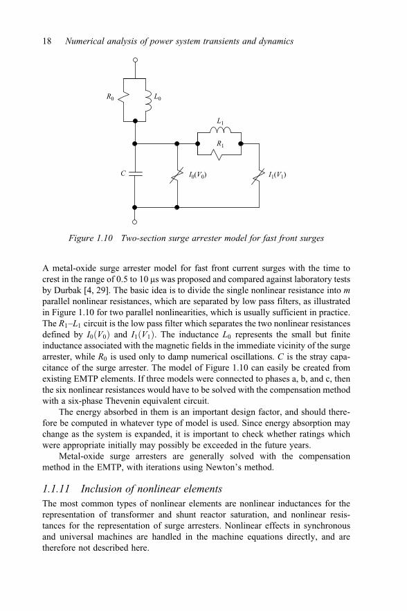
A metal-oxide surge arrester model for fast front current surges with the time tocrest in the range of 0.5 to 10 ms was proposed and compared against laboratory testsby Durbak [4, 29]. The basic idea is to divide the single nonlinear resistance into mparallel nonlinear resistances, which are separated by low pass filters, as illustratedin Figure 1.10 for two parallel nonlinearities, which is usually sufficient in practice.The R1–L1 circuit is the low pass filter which separates the two nonlinear resistancesdefined by I0ðV0Þ and I1ðV1Þ. The inductance L0 represents the small but finiteinductance associated with the magnetic fields in the immediate vicinity of the surgearrester, while R0 is used only to damp numerical oscillations. C is the stray capa-citance of the surge arrester. The model of Figure 1.10 can easily be created fromexisting EMTP elements. If three models were connected to phases a, b, and c, thenthe six nonlinear resistances would have to be solved with the compensation methodwith a six-phase Thevenin equivalent circuit.

The energy absorbed in them is an important design factor, and should there-fore be computed in whatever type of model is used. Since energy absorption maychange as the system is expanded, it is important to check whether ratings whichwere appropriate initially may possibly be exceeded in the future years.

Metal-oxide surge arresters are generally solved with the compensationmethod in the EMTP, with iterations using Newton’s method.

1.1.11 Inclusion of nonlinear elementsThe most common types of nonlinear elements are nonlinear inductances for therepresentation of transformer and shunt reactor saturation, and nonlinear resis-tances for the representation of surge arresters. Nonlinear effects in synchronousand universal machines are handled in the machine equations directly, and aretherefore not described here.

R0

C

L0

L1

R1

I0(V0) I1(V1)

Figure 1.10 Two-section surge arrester model for fast front surges


Usually, the network contains only a few nonlinear elements. It is thereforesensible to modify the well-proven linear methods more or less to accommodatenonlinear elements, rather than to use less efficient nonlinear solution methods forthe entire network. This has been the philosophy which has been followed in theEMTP. Three modification schemes have been used over the years, namely

● current-source representations with time lag Dt (no longer used),● compensation methods, and● piecewise linear representations.

1.1.11.1 Current-source representation with time lag DtAssume that the network contains a nonlinear inductance with a given flux/currentcharacteristic lðiÞ, and that the network is just being solved at instant t. All quan-tities are therefore known at t � Dt, including flux lðt � DtÞ, which is found byintegrating the voltage across the nonlinear inductance up to t � Dt. Provided Dt issufficiently small, one could use lðt � DtÞ to find a current iðt � DtÞ from thenonlinear characteristic, and inject this as a current source between the two nodes towhich the nonlinearity is connected for the solution at instant t. In principle, anynumber of nonlinearities could be handled this way.

Since this method is very easy to implement, it may be useful in special cases,provided that the step size Dt is sufficiently small. It is not a built-in option in anyof the available EMTP versions.

1.1.11.2 Compensation methodIn earlier version of the EMTP, the compensation method worked only for a singlenonlinearity in the network, or in case of more nonlinearities, if they were allseparated from each other through distributed-parameter lines. It appears that thetype-93 nonlinear inductance in the EMTP [3] still has this restriction imposed onit, but for most other types, more nonlinearities without travel time separation areallowed now.

The extension of the compensation method to more than one nonlinearity wasfirst implemented for metal-oxide surge arresters, and later used for other nonlinearelements as well.

In comparison-based methods, the nonlinear elements are essentially simulatedas current injections, which are super-imposed on the linear network after a solu-tion without the nonlinear elements has first been found.

When the EMTP tries to calculate the Thevenin equivalent resistance for thenonlinear branch by injecting current into node m, a zero diagonal elementwill be encountered in the nodal conductance matrix if the nonlinear elementis removed from the circuit during a simulation. Then, the EMTP will stop withthe error message ‘‘diagonal element in node-m too small.’’ The remedy in thiscase is: represent the nonlinear branch as a linear branch in parallel with a(modified) nonlinear branch. The EMTP manual also suggests the insertion ofhigh-resistance path where needed, but warns that the resistance values cannot bearbitrarily large.


1.1.12 TACS1.1.12.1 IntroductionThe program called TACS was developed in 1977 by late L. Dube [15]. In 1983/84,Ma Ren-Ming did a thorough study of the code, and made major revisions in it,particularly with respect to the order in which the blocks of the control system aresolved [30].

TACS was originally written for the simulation of HVDC converter controls,but it soon became evident that it had much wider applications. It has been used forthe following simulations for example.

(a) HVDC converter controls,(b) excitation systems of synchronous machines,(c) current limiting gaps in surge arresters,(d) arcs in circuit breakers.

TACS can be applied to the devices or phenomena which cannot be modeleddirectly with the existing network components in the EMTP.

Control systems are generally represented by block diagrams which show theinterconnections among various control system elements, such as transfer functionblocks, limiters. A block diagram representation is also used in TACS because itmakes the data specification simple. All signals are assigned names which aredefined by six alphanumeric characters (blank is included as one of the characters).By using the proper names for the input and output signals of blocks, any arbitraryconnection of blocks can be achieved. There exists no uniform standard fordescribing the function of each block in an unambiguous way, except in the case oflinear transfer functions. Users of the EMTP should be aware of this.

The control systems, devices and phenomena modeled in TACS, and theelectric network are solved separately at this time. Output quantities from the net-work solution can be used as input quantities in TACS over the same time step,while output quantities from TACS can become input quantities to the networksolution only over the next time step. TACS accepts as input network voltage andcurrent sources, node voltages, switch currents, status of switches, and certaininternal variables such as rotor angles of synchronous machines. The networksolution accepts output signals from TACS as voltage or current sources (if thesources are declared as TACS controlled sources), and as commands to open orclose switches (if the switch is a thyristor or a TACS controlled).

The present interface between the network solution and TACS is explained inthe following section.

1.1.12.2 Interface between TACS and electric networksTo solve the models represented simultaneously with the network is more com-plicated than for models of power system components such as generators ortransformers. Such components can essentially be represented as equivalent resis-tance matrices with parallel current sources, which fit directly into the nodal net-work (1.2). The equations of control system are quite different in that aspect. Theirmatrices are unsymmetrical and they cannot be represented as equivalent networks.


Because of these difficulties, L. Dube decided to solve the electric network(briefly called NETWORK from here on) and the TACS models (briefly calledTACS from here on) separately. This imposes limitations which the user shouldbe aware of. As illustrated in Figure 1.11, the NETWORK solution is firstadvanced from ðt � DtÞ to t as if TACS would not exist directly. There is anindirect link from TACS and NETWORK with a time delay of Dt, inasmuch asNETWORK can contain voltage and current sources defined between ðt � DtÞand t which were computed as output signals in TACS in the preceding stepbetween ðt � 2DtÞ to ðt � DtÞ. NETWORK also receives commands for openingand closing switches at time t, which are determined in TACS in the solutionfrom ðt � 2DtÞ to ðt � DtÞ. In the latter case, the error in the network solution dueto the time delay of Dt is usually negligible. First, Dt for this type of simulation isgenerally small, say, 50 ms. Second, the delay in closing a thyristor switchcompensated by the converter control, which alternately advances and retards thefiring of thyristor switches to keep the current constant in steady-state operation.With continuous voltage and current source functions coming from TACS, thetime delay can become more critical, however, and the users are aware of itsconsequences. Cases have been documented where this time delay of Dt cancause numerical instability, i.e., in modeling the arc of circuit breakers withTACS [31].

Once NETWORK has been solved, the network voltages and currents specifiedas input to TACS are known between ðt � DtÞ to t. No time delay occurs in this partof the interface, except that TACS itself has built-in delays which may not alwaysbe transparent to the user.

NETWORKsolution from

t – Δt to t

TACSsolution from

t – Δt to t

Timedelay Δt

Node voltages, branchcurruents, etc., betweent – Δt and t used asinput to TACS

Voltage and current sources,time-varying resistance, etc.,between t – Δt and t used asinput to NETWORK in nextstep from t to t + Δt

Figure 1.11 Interface between NETWORK and TACS solution


1.1.13 MODELS (implemented in the ATP-EMTP)MODELS is a kind of a simulation language to study electromagnetic transients,with focus on the needs answered by the language for EMTP use. MODELS wasdeveloped by L. Dube in 1992 [32] to allow users to describe electrical componentsand control systems that otherwise could not be represented easily using regularcomponents and control functions of EMTP. MODELS also provides a standardizedinterface at the modeling level for connecting user-supplied external programs toEMTP.

1.1.13.1 Design objectives of MODELSThe design objectives that have directed the construction of the MODELS languageare the following:

(a) to give the possibility directly to the users of EMTP to develop models ofnetwork components and control algorithms which cannot be built easily withthe set of basic elements available in EMTP and TACS;

(b) to provide to the user the flexibility of a full programming language withoutrequiring the users to interact with EMTP at the programming level;

(c) to let the user describe not only how a component operates, but also how theinitial state (initial values and initial history) of the component is established,at a detail level selected by the user;

(d) to provide standardized interface to EMTP defined at the modeling level interms of voltages, currents, and control quantities (as opposed to an interfacewhich would be defined at the programming level in terms of arrays of valuesand internal EMTP execution flow), giving directly to the user the possibilityof connecting external programs to EMTP for modeling of components,access to measurements, or interaction with equipment, without requiring theuser to have a programming knowledge if the internal operation of EMTP orto make any modification to the source code of EMTP.

In order to provide maximum power and flexibility when building models, itwas considered necessary to maintain the advantages offered by regular program-ming languages. In particular, the language had to include the followingpossibilities:

(a) separating the description of a component from its actual use in a simulation;(b) allowing the use of multiple instances of the same component, each possibly

supplied with different parameters, different inputs, or different simulationdirectives;

(c) providing a formal mechanism for the division of a large componentdescription into smaller procedures, for reduced model complexity, explicitidentification of interfaces, and functionality, easier testing, and use of pro-totyping during model development;

(d) providing a separate naming scope for each procedure, to allow the user toassign meaningful names to the variables used in a description;


(e) supporting the use of comments within a description, as an aid to producingmodels and procedures that are self-documenting:

(f) supporting the use of conditions and loops (if, while, for, etc.) for building thestructure of the execution flow of a procedure;

(g) providing a regular syntax for the use of variables, arrays, expressions, andfunctions.

1.1.13.2 Implementation of the design objectivesIn order to support the above design objectives, the simulation language MODELS hasbeen constructed as a Pascal-like procedural language with additional applications-specific syntax and functions for representing the continuous-time operation ofdynamic systems. Its grammar is keyword-directed and non-formatted.

In addition to the block diagram approach of TACS, MODELS accepts com-ponent descriptions in terms of procedures, functions, and algorithms. The user isnot limited to predefined set of components, but can build libraries of componentsand submodels as required by each application. Similarly, the user is not limited to aninput–output signal flow presentation, but can also combine this with numerical andlogical manipulation of variables inside algorithmic procedures.

The free format of the description and the possibility of using arbitrarily longnames facilitate self-documentation, valuable especially when large systems andteam work are of concern. Comments and illustrations can be introduced through-out a model description for clearer documentation.

Numerical and Boolean values are supported, in both scalar and array forms.Values are described using algebraic and Boolean expressions, differential equa-tions, Laplace transfer functions, integrals, and polynomials of derivatives. A largeselection of numerical and Boolean functions can be used inside expressions. Inaddition, simulations-specific functions provide access to the time parameters ofthe simulation and to past and predicted values of the variables of a model. Addi-tional functions can be defined by the user, in the form of parameterized expres-sions, point lists, and externally programmed functions.

Dynamic changes in the operation of a model are described by use of IF,WHILE, and FOR directives applied to groups of statements and to the use ofsubmodels. Groups of simultaneous linear equations are solved in matrix form,using Gaussian elimination. Arbitrary iteration procedures can also be specified bythe user for solving groups of simultaneous nonlinear equations. All other valueassignments are calculated and applied sequentially in the order of their definitionsin the model description.

The description of a model can be written directly as data in an EMTP datacase, or accessed at simulation time from libraries of pre-written model files.

Self-diagnosis is especially important when large models have to be set up,debugged, and fine-tuned. Detection of the existence of possible misoperation canbe built directly into the model by the user, forcing an erroneous simulation to behalted via the ERROR statement with clear indication of the problem that occurred.Warnings and other observations can also be recorded during the simulation forlater analysis.


The language provides a mechanism for explicitly structuring a system intoseparate sub-components, supporting the definition and use of embedded sub-models. The same model can be used at multiple locations in a simulation, withparameters, inputs, outputs, and simulation directives specified individually foreach use.

The simulation of each instance of a model is conducted in two phases. Theinitialization phase establishes initial values and initial history when the instance isfirst accessed. The model then repeatedly updates the values of the variables and ofthe accumulated history of the instance, in function of the changing values appliedto its inputs. A detailed procedure can be defined to describe separately with fullflexibility both the initialization and the operation of the model.

External programs can be directly defined and used as a model via a standar-dized interface, simply linked with the program without requiring any modificationto be made to the EMTP source code. The interface is defined by the user in termsof voltages, currents, and control variables of the simulation. No knowledge of theEMTP at the programming level is required.

1.1.14 Power system elements prepared in EMTPTable 1.1(a) summarizes various power system elements, and Table 1.1(b) showssupporting routines prepared in the original EMTP (Mode 31, April 1982 [3]). Thesupporting routines are a subroutine installed in the EMTP and calculate parametersrequired for the power system elements such as a transformer and a transmissionline in Table 1.1(a).

1.1.15 Basic input dataNowadays, any numerical simulation tool provides a user-friendly graphic interfaceof input (and output) data. Such an interface makes data input much easier from theusers’ viewpoint. At the same time, however, the users miss to catch physicalmeaning of each input data. It happens quite often that an input value is smaller orlarger by 103 or 106.

In this section, basic input data are described for a simulation of a switchingtransient in a circuit of Figure 1.12 in the input data format specified in the originalBPA EMTP [3] so that a use can catch the physical meaning of the input data.

Figure 1.13(a) shows the input data necessary for the simulation. The dataset, however, is not easy to understand for the user except an experienced one.

E = 100 V

R = 100 Ω

L = 1800 mH

TERRA

NODE_A

NODE_B

Figure 1.12 A transient on an R-L circuit


Figure 1.13(b) shows a more user-friendly version of the data set with in-linecomments explaining each data. Figure 1.14 gives the EMTP output to the inputdata in Figure 1.13. In Figures 1.13(b) and 1.14, ‘‘C’’ in the first column indicatesthat the line is for comments but not for the input data. 1 to ˙ in Figure 1.14 areidentical to those in Figure 1.13(b).

(a)

(b)

Figure 1.13 EMTP input data: (a) input data, (b) with in-line comments


The basic structure of the input data of the EMTP is

(1) BIGIN NEW DATA CASE: shows a new data set or the end of the data set;1 and ˙

(2) MISC (miscellaneous) data: to specify I/O formats; 2 and 3

(3) BRANCH data: data for the branch specified by two nodes; 4 and 5

(4) SWITCH data: data for a switch (no switch in this example)(5) SOURCE data: data for a source; 8(6) OUTPUT data: to specify the output; 0(7) PLOT data: to specify graphs of calculated results (not used in this example)(8) BLANK cards: to be inserted in between the data (2) to (7); 6, 7, 9, ˆ, ˜,

˘ in Figure 1.13.

(a)

Figure 1.14 (Continued )


Each data line is composed of 80 columns as shown in Figure 1.15. It should benoted that each column is specified to a specific data name or value. Thus, a usershould be very careful of the name, or of the value being correctly positioned in thespecified columns. This is a problem and a difficulty of producing a data set in theoriginal EMTP, and a reason for a user-friendly graphic interface has been providedin the EMTP-ATP, EMTP-RV, and PSCAD.

(b)

Figure 1.14 EMTP output: (a) input data copied by EMTP, (b) output


(1) M

ISC

dat

a

18

916

1724

2532

3340

4148

4956

DEL

TAT

TMA

XX

OPT

CO

PTEP

SILN

TOLM

AT

TSTA

RT

E8.0

E8.0

E8.0

E8.0

E8.0

E8.0

E8.0

18

916

1724

2532

3340

4148

4956

5764

6572

73

80

IOU

TIP

OLT

IDO

UB

LK

SSO

UT

MA

XO

UT

IPU

NM

EMSA

VIC

AT

NEN

ERG

IPR

SUP

I8I8

I8I8

I8I8

I8I8

I8I8

(2) B

RA

NC

H d

ata

123

89

1415

2627

3233

3839

4445

7980

ITY

-PE

node

nam

eno

de n

ame

refe

renc

e na

me

bran

ch d

ata

I-O

UT

NO

DE_

AN

OD

E_B

R [Ω

]L

[mH

]C

[μF]

I2A

6A

6A

6A

6A

6E6

.2E6

.2I1

Ex. 1

NO

DE_

1N

OD

E_2

1.2

Ex. 2

-1N

OD

E_A

TER

RA

100.

1800

.EX

. 2-2 N

OD

E_A

100.

1800

.Ex

. 3B

US_

1B

US_

210

.0.

05Ex

. 4IN

OU

T1.

5.1

.65

Ex. 5 1

NO

DE1

AN

OD

E1B

0.1

1.0

0.01

Ex. 6

IN_A

OU

T_A

1.5

0.1

1.2

IN_B

OU

T_B

IN_A

OU

T_A

IN_C

OU

T_C

IN_A

OU

T_A

2 3 4

Fig

ure

1.15

(Con

tinu

ed)

(3) S

WIT

CH

dat

a12

38

914

1524

2534

ITY

-

PE

node

nam

e

node

nam

e

time

to c

lose

T clos

e [s]

time

to o

pen

T open

[s]

SWIT

_1SW

IT_2

I2A

6A

6E1

0.0

E10.

0

Ex. 1

IN_A

SIN

_A.0

005

.002

(4) S

OU

RC

E da

ta12

38

9

1011

20

21

3031

40

41

5051

60

61

7071

80

(a)

ITY

-PE

(b)

node

nam

e(a

)V

/I(c

)A

MPL

I-TU

DE

(d)

FREQ

UEN

-C

Y

(e)

T 0 [se

c]q 0

[deg

ree]

(f)

only

for

TYPE

13,

14

A1

(f)

only

for

TYPE

13

T 1 [s]

(g)

T star

t [s]

for

TYPE

≠1,1

0

(h)

T stop

[s]

I2A

6I2

E10.

6E1

0.6

E10.

6E1

0.6

E10.

6E1

0.6

E10.

6

Ex. 1

-1

11V

OLT

_A10

00.

Ex. 1

-211

VO

LT_A

−11.

5Ex

. 2-1

11V

OLT

_A10

0..0

05Ex

. 2-2

12B

US_

2−1

−50.

.002

Ex. 3

-113

BU

S_A

100.

4.E−

650

.30

.E−6

40.E

−6Ex

. 3-2

13B

US_

A10

00.

2000

.50

.E−6

Ex. 4

-114

GEN

E_A

100.

50.

45.

Ex. 4

-214

GEN

E_B

100.

50.

45.

−1.

Ex. 4

-314

GEN

E_C

100.

50.

.002

51

Fig

ure

1.15

Bas

icst

ruct

ure

ofth

eE

MT

Pin

put

data

Now each data set, (2) to (6), is explained.

(1) BIGINDNEWDDATADCASE (19 characters, D ¼ space)1 To show data case and also a new data set in (2) to (7).

(2) MISC data2 First MISC data: explanation given in the line right above the data– DELTAT ¼ time step Dt in sec. [s], to be in columns 1st to 8th (total

8 characters).

example: 2E � 3 ¼ 2 ms

– TMAX ¼ maximum observation time in sec., 9th to 16th columns(8 characters).

– XOPT ¼ input format of an inductance. When it is made ‘‘blank’’ (¼ 0),defaulted format which means that the inductance value should be in theunit of [mH]. In this chapter, XOPT, which defines the unit (mH or W) ofthe inductance, is kept to be ‘‘blank.’’ XOPT is to be input in the columns17th to 24th.

– COPT ¼ input format of a capacitance. For COPT is ‘‘blank’’ (or zero),the capacitance value should be given in the unit of [mF]. In this chapter,it is kept ‘‘blank.’’ The data COPT in 25th to 32nd columns.

– EPSLN, TOLMAT ¼ variables related to the inverse calculation ofadmittance matrix, and to judge the singularity. These are neglected inthis example.

– TSTART ¼ the time to start a transient simulation, neglected in thisexample.3 Second MISC data: eight columns for every data

– IOUT ¼ sampling span of calculated results, i.e., the results are printedout for every Dt when IOUT ¼ 1. When IOUT ¼ 10, printout of theresults for every 10 � Dt. Thus, IOUT ¼ TMAT/DELTAT. 9th to 16thcolumns.

– IPLOT ¼ same as IOUT but for curve plotting. When IPLOT is definednegative, no curve plotting.

– IDUBLE ¼ 0: no output of the circuit connection diagram.

¼ 1: output circuit connection diagram.

In general, keep IDOUBLE ¼ 1 to check the circuit connection is corrector not.

– KSSOUT ¼ 0: no output of the steady-sate solution for t 0.

¼ 1: output the steady-state solution. When TSTART < 0, thesteady state is calculated to start a transient calculation.

– MAXOUT ¼ 0: no output of maximum voltages and currents.

¼ 1: The maximum voltages and currents are output after atransient simulation.


– IPUN ¼ 0: no output of node voltages and branch currents at t ¼ Tmax

which are used in the next transient in the same circuit.Also, there are the following MISC data which are required when a

special calculation or a specific output is necessary. In most cases, justleave them ‘‘blank.’’

MEMSAV ¼ memory save, ICAT ¼ plot file save, NENERG ¼statistical surge calculation, IPRSUP ¼ output of intermediate results.

(3) BANCH data4, 5 BRANCH data(a) ITYPE: 1st and 2nd columns

ITYPE is the data to specify if the branch data are lumped parameters ora distributed line.

ITYPE ¼ 0 or blank: lumped � parameter circuit

¼ negative value: distributed � parameter line

�1: for the first phase; �2: for the second phase; etc:

(b) node names: 3rd to 14th columnsIn the circuit of Figure 1.12, voltage source eðtÞ and inductance L are

grounded to the zero potential node (TERRA in the EMTP which isexpressed by ‘‘blank’’). In the BRANCH data, the six columns from the3rd to the 8th column (‘‘<BUS1>’’ in the comment line) are used for thenode name of the sending end of a branch, and the next six columns (fromthe 9th to the 14th column, ‘‘<BUS2>’’ in the comment line) are used forthe other end of the branch.

(c) Copied branch<BUS3> (from the 14th to the 19th column) and <BUS4> (from the

20th to 25th column) columns are used when the branch data for <BUS1>to <BUS2> branch are copied from <BUS3> to <BUS4> branch data.

(d) Branch dataBecause the branch from NODE_A to NODE_B is a resistance as

illustrated in Figure 1.12, the value of the resistance, 100 W, is to beinput in the columns from the 27th to the 32nd as shown in Figure 1.13.There exists an inductance between NODE_B to ground (TERRA ¼blank), and the value of the inductance 1,800 mH is input in the columnsfrom the 33rd to the 38th corresponding to the comment <L mH> in thecomment line.

Similarly if there is a capacitance in a circuit, its value is input in thecolumns from the 39th to the 44th corresponding to <C mF> in thecomment line.

(e) Series circuit of lumped-parameter elements, R, L, and C can be input inone BRANCH data line. If there is no capacitance, then the columns cor-responding to the capacitance should be made ‘‘blank.’’

Some examples are given in Figure 1.15 (2) corresponding to thecircuits illustrated in Figure 1.16.


(f) Multiphase p circuitBy setting ITYPE to be positive sequential numbers similarly to a

multiphase distributed line, p circuit equivalence of a multiphase dis-tributed line is input, i.e.,

ITYPE ¼ 1: first phase data, 2: the second phase, etc.

6 BLANK CARD: to show the end of the BRANCH data explained above.

(a)

(b)

(c)

(d)

(e)

Ea

Eb

Ec

IN_A

IN_B

IN_C

IN_AS0.1 mH

0.65 μF

OUT_A

OUT_B

OUT_C

0.1 ΩNODE1A NODE1B1 mH

C/2C/2

C = 0.01 μF

0.65 μF1.5 Ω

IN OUT0.1 mH

0.05 μF10 Ω

BUS_1 BUS_2

C = 1.2 μF

NODE_1 NODE_2

Figure 1.16 Examples of BRANCH: (a) Ex. 1 Capacitance C, (b) Ex. 3 R-C seriescircuit, (c) Ex. 4 R-L-C series circuit, (d) Ex. 5 p-equivalence,(e) Three-phase R-L-C circuit


(4) Switch data‘‘SWITCH’’ data are to specify the type of a switch, the closing time, the

opening time, etc. The columns 1–2 of the SWITCH data are to define thetype of switches as explained in Section 1.1.9. For example,

ITYPE ¼ 0 (or blank): ordinary switches for which the voltage drop iszero when closed, and the current is zero when open. The ordinary switchesinvolve the following options (called ‘‘Class’’).

Class 1 ¼ time-controlled switch (circuit breaker pole) which requires theinput data of closing time ‘‘Tclose’’ and opening time ‘‘Topen’’ as illustrated inFigure 1.15 (3).

The switch is open originally, close at t � Tclose and tries to open aftert � Topen. There are two options; see Figure 1.6 in Section 1.1.9 (2).

Option A: the opening is successful as soon as the current isw has gone throughzero detected by a sign change in isw.

Option B: the opening is successful as soon as jiswj < current margin or assoon as isw has gone through zero.

Class 2 ¼ voltage-controlled switch (gap) which requires the input data‘‘Vflash.’’ When the voltage across the switch (open) terminals exceeds Vflash,then the switch is closed.

Class 3a ¼ statistic switch: time-controlled switch where the closing time isa random variable.

Class 3b ¼ systematic switch: time-controlled switch where the closingtime is systematically varied.

Class 4 ¼ measuring switch: permanently closed, just for monitoring cur-rent, power, or/and energy.

Class 5 ¼ TACS controlled switch.

In the example illustrated in Figure 1.13, there is no switch although a switchis shown in Figure 1.12. This is because the switching operation is included inthe voltage source E which is connected to NODE_A at t ¼ 0.

7 BLANK CARD: to show the end of the switch data.(5) SOURCE data

8 SOURCE data: composed of ITYPE, NODE name, V=I , AMPLITUDE,FREQUENCY, etc.(a) ITYPE: 1st and 2nd columns to specify the type of sources.

ITYPE ¼ 11: dc source shown as Ex. 1 in Figure 1.15 (4) andFigure 1.17(a-1) and (a-2). Remind that the voltage (or current) at t ¼ 0is zero unless the initial conition is given in the circuit. Thus, the voltage(or current) reaches the given amplitude at t ¼ Dt (time step) as shownin Figure 1.17(a).ITYPE ¼ 12: ramp function with linear rise from t ¼ 0 to t ¼ T0, andconstant apmlitude thereafter; see Ex. 2 in Figures 1.15 (4) and 1.17(b).ITYPE ¼ 13: ramp function with linear decay; see Ex. 3-1 in Figure 1.15(4) and Figure 1.17(c-1). If A1>AMPLITUDE as in Ex. 3-2 inFigure 1.15(4), then the waveform in Figure 1.17(c-2) is given.


ITYPE ¼ 14: sinusoidal function, see Ex. 4 in Figures 1.15 (4) and 1.17(d).In Ex. 4-2, Tstart < 0 means that the circuit is in a steady state for t < 0as shown in dotted line (Ex. 4-2) in Figure 1.17(d). Unless this is done,no printout of a steady-state solution.In Ex. 4-3, A1 > 0 means that the sinusoidal function is defined by

f ðtÞ ¼ AMPLITUDE � cos½2pf ðt þ T0Þ�; T0 in sec:

When A1 ¼ 0: f tð Þ ¼ AMPLITUDE � cos 2pft þ q0½ �, q0 in degrees.

(a-1) (c-1)

(a-2) (c-2)

(b) (d)

0

v(t)

[V]

100

–100

t

Ex. 4-1

= Ex. 4-3

Ex. 4-2

5 10 15 20 [ms]

–50 A

T0 = 5 ms

0.002 = 2 ms0

v(t)

[V]

Ex. 2-2

Ex. 2-1

0

v(t)

[V]

T0 = 0t

T1 = 50 μs

AMPLITUDE= 1,000 V

A1 = 2,000 V

AMPLITUDE = 1.5A

1.5

0

[A]

4 μs

100

0

v(t)

[V]

30 μs 40 μsTSTOP

T0 T1AMPLITUDE = 1,000 V

1,000

0

v(t)

i(t)

[V]

Δt

Δt

t

AMPLITUDE = 100 V

Figure 1.17 Various source waveforms: (a-1) Ex. 1-1 Voltage source, (a-2) Ex. 1-2Current source, (b) Ex. 2, (c-1) Ex. 3-1, (c-2) Ex. 3-2, (d) Ex. 4


(b) Node name: columns 3–8 to specify the node to which a source is con-nected. The other node of the source is grounded (to TERRA).

(c) V=I : columns 9–10, V=I ¼ 0 (blank or positive integer): voltage source

¼ negative integer: current source, see Ex. 2-2in Figure 1.15 (4).

(d) AMPLITUDE: columns 11–20 to give the amplitude of a voltage [V]or current [A].

In the case of a dc source (ITYPE ¼ 11), the following data are notnecessary.

(e) FREQUENCY: columns 21–30 to specify the ac source frequency, onlyfor ITYPE ¼ 14.

(f) T0 s½ � or q0 deg:½ �: columns 31–40For ITYPE ¼ 14 (ac source): see the above explanation in (a).For ITYPE ¼ 12: time T0 to reach amplitude, see Ex. 2 in Figures 1.15and 1.17(b).For ITYPE ¼ 13: time T0 to the peak (amplitude), see Ex. 3-1 inFigures 1.15 (4) and 1.17(c-1). If T0 is given as ‘‘blank,’’ then, data forA1 and T1 are required.

(g) A1: columns 41–50 only for ITYPE ¼ 13 and 14, T1: columns 51–60only for ITYPE ¼ 13.For ITYPE ¼ 14: see (a)For ITYPE ¼ 13: linear rise for positive A1 at t ¼ T1 greater thanAMPLITUDE, see Ex. 3-2 in Figures 1.15 (4) and 1.17(c-2).

(h) Tstart: columns 71–80, blank in general. If a positive value of Tstop isgiven, then source e tð Þ ¼ 0 (or i tð Þ ¼ 0) at t ¼ Tstop.9 BLANK CARD: to end the SOURCE data.

(6) OUTPUT data0 OUTPUT data: to specify the node voltage output of an EMTP simulation.

In this example (see 0 in Figures 1.13 and 1.14), the voltage at NODE_A isprinted out. For a branch current and a branch voltage, the output is requestedat the 80th column of BRANCH data; see data 4 for a branch current output,and data 5 for a branch voltage (NODE_B to TERRA) in Figure 1.14(a).

The results output are shown in Figure 1.14(b).ˆ BLANK CARD: to end the OUTPUT data˜ BLANK CARD: to end the PLOT data¯ BLANK CARD: to end this data case˘ BLANK CARD: to show no more input data

Explained in the above is only a very basic component in the EMTP. Thereare many other components and functions as described in the previoussections. For example, a user-defined source is prepared as a SOURCE data(ITYPE ¼ 1 to 10). When a field test result is to be simulated, an appliedvoltage (or current) in the test is used as a SOURCE data by transferring themeasured voltage waveform to a PC in an electronic format.


The basic data format of a BRANCH data shown in Figures 1.13 and 1.14 isvery tight. To avoid this, a high precession format of a BRANCH data isprepared as shown in Figure 1.18. To use this format, ‘‘$VINTAGE, 1’’ datais to be input before the BRANCH data, and ‘‘$VINTAGE, 0’’ comes after thedata to declare the end of the BRABCH data.

More details of the input format and the output can be found in [3]. Also, anumber of test cases are described in [33].

1.2 Numerical electromagnetic analysis

It is hard to handle a transient associated with non-TEM mode propagation byconventional circuit theory-based tools such as the EMTP, because the tools arebased on TEM mode propagation. To overcome the problem, a numerical electro-magnetic analysis (NEA) method looks most promised among existing transientanalysis approaches for it solves Maxwell’s equation directly without assumptionsoften made for the circuit theory-based approach.

This section describes the basic theory of two representative methods, i.e.,method of moment (MoM) and finite-difference time-domain (FDTD) method, ofthe NEA.

1.2.1 IntroductionAn NEA method is becoming a powerful tool to solve surge phenomena in powersystems such as an induced lightning surge, a surge response of a grounding elec-trode and corona pulse propagation on a gas-insulated bus which are very hard tosolve by an existing circuit theory-based tool such as the EMTP, because thesesurge phenomena involve transverse magnetic (TM) and transverse electric (TE)modes of wave propagation rather than TEM mode propagation which is the basisof the existing circuit theory-based tool. Also the circuit parameters, which arenecessary to analyze a phenomenon by the circuit theory-based tool, are quite oftennot clear or not available. Because the NEA method solves Maxwell’s equationdirectly based on the boundary conditions and the physical and geometricalparameters of a surge phenomenon to be solved, it requires no circuit parameter.Also, the method can solve the TE, TM, and TEM mode propagation without anydifficulties.

$ VINTAGE, 11 2 3 8 9 14 15 20 21 26 27 42 43 58 59 74 75 79 80

ITYPE

node

name

node

namereference branch branch parameters

IOUT

NODE_1 NODE_2node

name

node

nameR [Ω] L [mH] C [μF]

I2 A6 A6 A6 A6 E16.0 E16.0 E16.0 I1

$ VINTAGE, 0

Figure 1.18 A high precision format of a BRANCH data


The IEE Japan Working Group of Numerical Electromagnetic AnalysisMethod for Surge phenomena (WG here after, convenor: Ametani) started in April2004 [34] and CIGRE WG C4.501 (convenor: Ametani) started in October 2009[35] has surveyed the basic theory and assumption of various approaches of theNEA published in literatures, and has collected the application examples. Fur-thermore, bench-mark tests are carried out by the WG members and finally the WGhas made clear the applicable limit, advantage, and disadvantage of each approach.

This section summarizes the works related to NEA including the WGactivities.

1.2.2 Maxwell’s equationsBefore NEA methods are explained, Maxwell’s equations, which are the basis ofelectromagnetics, are described. There are two types of the equations: one is in timedomain and the other is in frequency domain.

In the time domain, Maxwell’s equations are expressed as

r� E r; tð Þ ¼ � @B r; tð Þ@t

ð1:19Þ

r �H r; tð Þ ¼ @D r; tð Þ@t

þ J r; tð Þ ð1:20Þ

r �D r; tð Þ ¼ r r; tð Þ ð1:21Þr � B r; tð Þ ¼ 0 ð1:22Þ

where E(r, t): electric field, H(r, t): magnetic field, D(r, t): electric flux density,B(r, t): magnetic flux density, J(r, t): conduction current density, r(r, t): volumecharge density, each at the space point r and at the time t.

Equation (1.19) represents Faraday’s law, and (1.20) represents Ampere’s law.Equations (1.21) and (1.22) represent Gauss’s law for electric and magnetic fields,respectively.

In the frequency domain, Maxwell’s equations are expressed as

r� E rð Þ ¼ �jwB rð Þ ð1:23Þr �H rð Þ ¼ J rð Þ þ jwD rð Þ ð1:24Þr �D rð Þ ¼ r rð Þ ð1:25Þr � B rð Þ ¼ 0 ð1:26Þ

where j: imaginary unit, w: angular frequency.The relations of the electric and magnetic flux densities to the electric and

magnetic fields are given as

D rð Þ ¼ eE rð Þ ¼ ere0E rð Þ ð1:27ÞB rð Þ ¼ mH rð Þ ¼ mrm0H rð Þ ð1:28Þ


where e0: permittivity of vacuum ¼ 8.854 �10�12 F/m,m0: permeability of vacuum ¼ 4p�10�7 H/m, er: relative permittivity of medium,mr: relative permeability of medium, e: permittivity of medium,m: permeability of medium.

In a conductive medium, the following relation of the electric field to the con-duction current density, Ohm’s law, is fulfilled:

J rð Þ ¼ sE rð Þ ð1:29Þ

where s is the conductivity of the medium.

1.2.3 NEA method1.2.3.1 Various methodsTable 1.2 categorizes various methods of NEA which are presently used.

The method of moments (MoM) in the frequency and time domains [36–41],and the FDTD method [42, 43], both for solving Maxwell’s equations numerically,have frequently been used in calculating surges on power systems. Applications ofthe finite element method (FEM) and the transmission matrix method (TLM) tosurge calculations have been rare at present. The MoM and the FDTD methods are,therefore, two representative approaches in surge calculations.

1.2.4 Method of Moments in the time and frequency domains1.2.4.1 MoM in the time domainThe MoM in the time domain [36, 37] is widely used in analyzing responses ofthin-wire metallic structures to external time-varying electromagnetic fields. Theentire conducting structure representing the lightning channel is modeled by acombination of cylindrical wire segments whose radii are much smaller than thewavelengths of interest. The so-called electric-field integral equation for a perfectlyconducting thin wire in air as in Figure 1.19, assuming that current I and charge qare confined to the wire axis (thin-wire approximation) and that the boundarycondition on the tangential electric field on the surface of the wire (this field mustbe equal to zero) is fulfilled, is given by

s � Eincðr; tÞ ¼ m0

4p

ðC

s � s0

R

@Iðs0; t0Þ@t0

þ cs � R

R2

@Iðs0; t0Þ@s0

� c2 s � R

R3qðs0; t0Þ

2664

3775ds0 ð1:30Þ

where qðs0; t0Þ ¼ �Ð t0

�1@Iðs0;tÞ@s0 dt:

C is an integration path along the wire axis, Einc denotes the incident electricfield that induces current I, R ¼ r � r 0, r, and t denote the observation location (apoint on the wire surface) and time, respectively, r 0 and t 0 denote the source loca-tion (a point on the wire axis) and time, respectively, s and s0 denote the distancealong the wire surface at r and that along the wire axis at r 0, s, and s0 denote unit


Tab

le1.

2V

ario

usm

etho

dsof

NE

A

Par

titi

onSp

ace

Bou

ndar

y

Dis

cret

izat

ion/

dom

ain

Fin

ite

diff

eren

ceB

ound

ary

leng

thF

init

eel

emen

t

Tim

e-do

mai

nF

DT

DT

D-F

I3D

circ

uit

TL

MT

D-F

EM

MoM

(TW

TD

A)

Fre

quen

cy–

FI

––

FE

MM

oM

Bas

eeq

uati

onM

axw

ell

diff

eren

tial

Max

wel

lin

tegr

alM

axw

ell

char

acte

rist

icD

’Ale

mbe

rtso

luti

onF

ield

inte

gral

Cir

cuit

theo

ryex

tens

ion

Fea

ture

Eas

y prog

ram

min

gM

ulti

med

iaH

ard

prog

ram

Eas

ypr

ogra

mW

ide

appl

icat

ion

Sm

all

CP

U,n

onli

near

inti

me

dom

ain

vectors tangent to path C in (1.19) at r and r 0, m0 is the permeability of vacuum, andc is the speed of light. Through numerically solving (1.19), which is based onMaxwell’s equations, the time-dependent current distribution along the wirestructure (lightning channel), excited by a lumped source, is obtained.

The thin-wire time-domain (TWTD) code [36] (available from the LawrenceLivermore National Laboratory) is based on the MoM in the time domain. One ofthe advantages of the use of the time-domain MoM is that it can incorporate non-linear effects such as the lightning attachment process [38], although it does notallow lossy ground and wires buried in lossy ground to be incorporated.

1.2.4.2 MoM in the frequency domainThe MoM in the frequency domain [39] is widely used in analyzing the electro-magnetic scattering by antennas and other metallic structures. In order to obtain thetime-varying responses, Fourier and inverse Fourier transforms are employed. Theelectric-field integral equation derived for a perfectly conducting thin wire in air asin Figure 1.19 in the frequency domain is given by

�s � EincðrÞ ¼ jh4pk

ðC

Iðs0Þ k2s � s0 � @2

@s@s0

� �gðr; r0Þds0 ð1:31Þ

where gðr; r0Þ ¼ exp �jk r�r0j jr�r0j j

� �; k ¼ w ffiffiffiffiffiffiffiffiffim0e0

p; h ¼

ffiffiffiffim0e0

q:

w is the angular frequency, m0 is the permeability of vacuum, and e0 isthe permittivity of vacuum. Other quantities in (1.31) are the same as those in(1.30). Current distribution along the lightning channel can be obtained numericallysolving (1.31).

This method allows lossy ground and wires in lossy ground (for example,grounding of a tall strike object) to be incorporated into the model. The commer-cially available numerical electromagnetic codes [40, 41] are based on the MoM inthe frequency domain.

C(r)

s

s ¢

r ¢r

Origin

I (s′)

^

^

Figure 1.19 Thin-wire segment for MoM-based calculations. Current is confinedto the wire axis, and the tangential electric field on the surface of thewire is set to zero


1.2.5 Finite-difference time-domain methodThe FDTD method [42] employs a simple way to discretize Maxwell’s equations indifferential form. In the Cartesian coordinate system, it requires discretization of theentire space of interest into small cubic or rectangular-parallelepiped cells. Cells forspecifying or computing electric field (electric field cells) and magnetic field cellsare placed relative to each other as shown in Figure 1.20. Electric and magnetic fieldsof the cells are calculated using the discretized Maxwell’s equations given below.

Ezn i; j; k þ 1

2

� �¼ 1 � sði; j; k þ 1=2ÞDt= 2eði; j; k þ 1=2Þ½ �

1 þ sði; j; k þ 1=2ÞDt= 2eði; j; k þ 1=2Þ½ � � Ezn�1 i; j; k þ 1

2

� �

þ Dt=eði; j; k þ 1=2Þ1 þ sði; j; k þ 1=2ÞDt= 2eði; j; k þ 1=2Þ½ �

1DxDy

�Hy

n�12 i þ 1=2; j; k þ 1=2ð ÞDy � Hy

n�12 i � 1=2; j; k þ 1=2ð ÞDy

�Hxn�1

2 i; j þ 1=2; k þ 1=2ð ÞDx þ Hxn�1

2 i; j � 1=2; k þ 1=2ð ÞDx

24

35

ð1:32Þ

Hxnþ1

2 i; j � 12; k þ 1

2

� �¼ Hx

n�12 i; j � 1

2; k þ 1

2

� �þ Dt

mði; j � 1=2; k þ 1=2Þ1

DyDz

� �Ezn i; j; k þ 1=2ð ÞDz þ Ez

n i; j � 1; k þ 1=2ð ÞDz

þEyn i; j � 1=2; k þ 1ð ÞDy � Ey

n i; j � 1=2; kð ÞDy

" #

ð1:33Þ

Equation (1.32), which is based on Ampere’s law, is an equation updatingz component of electric field, Ez(i, j, k þ 1/2), at point x ¼ iDx, y ¼ jDy, andz ¼ (k þ 1/2)Dz, and at time t ¼ nDt. Equation (1.33), which is based on

H-field cell

Δz

Δx

ΔyEz (i, j, k + 1/2)

Hx (i, j – 1/2, k + 1/2)

Hx (i, j + 1/2, k + 1/2)

Hy (i + 1/2, j, k + 1/2)

Hy (i – 1/2, j, k + 1/2)

E-field cell

Ez (i, j – 1, k + 1/2)

Ez (i, j, k + 1/2)

Ey (i, j – 1/2, k + 1)

Ey (i, j – 1/2, k)

Hx (i, j – 1/2, k + 1/2)

E-field cell

H-field cell

Figure 1.20 Placement of electric-field and magnetic-field cells for solvingdiscretized Maxwell’s equations using the FDTD method


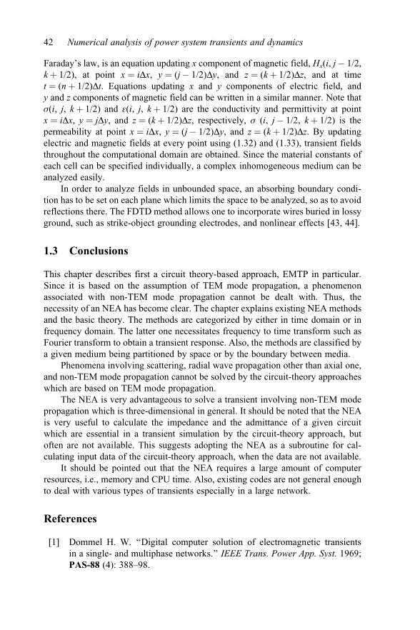
Faraday’s law, is an equation updating x component of magnetic field, Hx(i, j � 1/2,k þ 1/2), at point x ¼ iDx, y ¼ (j � 1/2)Dy, and z ¼ (k þ 1/2)Dz, and at timet ¼ (n þ 1/2)Dt. Equations updating x and y components of electric field, andy and z components of magnetic field can be written in a similar manner. Note thats(i, j, k þ 1/2) and e(i, j, k þ 1/2) are the conductivity and permittivity at pointx ¼ iDx, y ¼ jDy, and z ¼ (k þ 1/2)Dz, respectively, s (i, j � 1/2, k þ 1/2) is thepermeability at point x ¼ iDx, y ¼ (j � 1/2)Dy, and z ¼ (k þ 1/2)Dz. By updatingelectric and magnetic fields at every point using (1.32) and (1.33), transient fieldsthroughout the computational domain are obtained. Since the material constants ofeach cell can be specified individually, a complex inhomogeneous medium can beanalyzed easily.

In order to analyze fields in unbounded space, an absorbing boundary condi-tion has to be set on each plane which limits the space to be analyzed, so as to avoidreflections there. The FDTD method allows one to incorporate wires buried in lossyground, such as strike-object grounding electrodes, and nonlinear effects [43, 44].

1.3 Conclusions

This chapter describes first a circuit theory-based approach, EMTP in particular.Since it is based on the assumption of TEM mode propagation, a phenomenonassociated with non-TEM mode propagation cannot be dealt with. Thus, thenecessity of an NEA has become clear. The chapter explains existing NEA methodsand the basic theory. The methods are categorized by either in time domain or infrequency domain. The latter one necessitates frequency to time transform such asFourier transform to obtain a transient response. Also, the methods are classified bya given medium being partitioned by space or by the boundary between media.

Phenomena involving scattering, radial wave propagation other than axial one,and non-TEM mode propagation cannot be solved by the circuit-theory approacheswhich are based on TEM mode propagation.

The NEA is very advantageous to solve a transient involving non-TEM modepropagation which is three-dimensional in general. It should be noted that the NEAis very useful to calculate the impedance and the admittance of a given circuitwhich are essential in a transient simulation by the circuit-theory approach, butoften are not available. This suggests adopting the NEA as a subroutine for cal-culating input data of the circuit-theory approach, when the data are not available.

It should be pointed out that the NEA requires a large amount of computerresources, i.e., memory and CPU time. Also, existing codes are not general enoughto deal with various types of transients especially in a large network.

References

[1] Dommel H. W. ‘‘Digital computer solution of electromagnetic transientsin a single- and multiphase networks.’’ IEEE Trans. Power App. Syst. 1969;PAS-88 (4): 388–98.


[2] Dommel H. W., Scott-Meyer W. S. ‘‘Computation of electromagnetic tran-sients.’’ Proc. IEEE. Jul 1974; 62: 983–93.

[3] Scott-Meyer W. EMTP Rule Book. Portland, Oregon: Bonneville PowerAdministration (BPA); Apr 1982.

[4] Dommel H. W. EMTP Theory Book. Portland, Oregon: Bonneville PowerAdministration (BPA); 1986.

[5] Tinney W. F., Walker J. W. ‘‘Direct solution of sparse network equations byoptimally ordered triangular factorization.’’ Proc. IEEE. Nov 1967; 55:1801–9.

[6] Tinney W. F., Meyer W. S. ‘‘Solution of large sparse systems by orderedtriangular factorization.’’ IEEE Trans. Auto. Control. Aug 1973; AC-18:333–46.

[7] Schnyder O. ‘‘Druckstosse in Pumpensteigleitungen.’’ Schweiz Bauztg.1929; 94 (22): 271–86.

[8] Bergeron L. ‘‘Etude das variations de regime dans les conduits d’eau: Solutiongraphique generale.’’ Rev. Generale de L’hydraulique. 1935; 1: 12–69.

[9] Parmakian J. Waterhammer Analysis: New York: Dover; 1963.[10] Frey W., Althammer P. ‘‘The calculation of electromagnetic transients on lines

by means of a digital computer.’’ Brown Boveri Rev. 1961; 48 (5/6): 344–55.[11] Meyer W. S., Dommel H. W. ‘‘Numerical modeling of frequency-dependent

transmission parameters in an electromagnetic transients program.’’ IEEETrans. Power App. Syst. 1974; PAS-93: 1401–9.

[12] Semlyen A., Dabuleanu A. ‘‘Fast and accurate switching transient calcula-tions on transmission lines with ground return using recursive convolution.’’IEEE Trans. Power App. Syst. 1975; PAS-94: 561–71.

[13] Ametani A. ‘‘A highly efficient method for calculating transmission linetransients.’’ IEEE Trans. Power App. Syst. 1976; PAS-95; 1545–51.

[14] Marti J. R. ‘‘Accurate modeling of frequency-dependent transmission linesin electromagnetic transient simulations.’’ IEEE Trans. 1982; PAS-101 (1):147–55.

[15] Dube L., Dommel H. W. ‘‘Simulation of control systems in an electro-magnetic transients program with TACS.’’ IEEE PES PICA ConferenceRecord. 1977; 10: 266–71.

[16] Brandwajn V. Synchronous Generator Models for the Simulation of Elec-tromagnetic Transients. Ph.D. Thesis, University of British Columbia,Canada, Apr 1977.

[17] Carroll D. P., Flugan R. W., Kalb J. W., Peterson H. A. ‘‘A dynamic surgearrester model for use in power system transient studies.’’ IEEE Trans.Power App. Syst. 1972; PAS-91: 1057–67.

[18] Phadke A. G. (ed.). Digital Simulation of Electrical Transient Phenomena.IEEE Tutorial Course, Course Text 81, EH0173-5-PWR. Piscataway, NJ:IEEE Service Center; 1980.

[19] Avila-Rosales J., Alvarado F. L. ‘‘Nonlinear frequency-dependent trans-former model for electromagnetic transient studies in power systems.’’ IEEETrans. Power App. Syst. 1982; PAS-101: 4281–8.


[20] Frame J. G., Mohan N., Liu. T. ‘‘Hysterisis modeling in an electromagnetictransients program.’’ IEEE Trans. Power App. Syst. 1982; PAS-101: 3403–12.

[21] Lauw H. K., Meyer W. S. ‘‘Universal machine modeling for the presentationof rotating electric machinery in an electromagnetic transients program.’’IEEE Trans. Power App. Syst. 1982; PAS-101: 1342–51.

[22] Funabashi T., Sugimoto T., Ueda T. ‘‘A study on frequency characteristics ofa generator model for transformer transfer voltage simulation.’’ Int. Work-shop of High-Voltage Engineering (IWHV 99), paper HV-99-46, 1999.

[23] Shulz R. P., Jones W. D., Ewart D. N. ‘‘Dynamic models of turbine generatorsderived from solid rotor equipment circuits.’’ IEEE Trans. Power App. Syst.1973; PAS-92: 926–33.

[24] Cross G., Hall M. C. ‘‘Synchronous machine and torsional dynamics simu-lation in the computation of electromagnetic transients.’’ IEEE Trans. PowerApp. Syst. 1978; PAS-97: 1074–86.

[25] IEEE Subsynchronous Resonance Task Force. ‘‘First benchmark model forcomputer simulation of subsynchronous resonance.’’ IEEE Trans. PowerApp. Syst. 1999; PAS-96 (5): 1565–72.

[26] IEEE Working Group Report. ‘‘Recommended phasor-diagram for synchro-nous machines.’’ IEEE Trans. Power App. Syst. 1969; PAS-88: 1593–610.

[27] Kind D. ‘‘The equal area criterion for impulse voltage stress of practicalelectrode configurations in air.’’ ETZ-A. 1958; 79: 65–9.

[28] Tominaga S., Azumi K., Shibuya Y., Imataki M., Fujiwara Y., Nishikawa S.‘‘Protective performance of metal-oxide surge arrester based on the dynamicV-I characteristics.’’ IEEE Trans. Power App. Syst. 1979; PAS-98: 1860–71.

[29] Durbak D. W. ‘‘Zinc-oxide arrester model for first surges.’’ EMTP Newsletter.1985; 5 (1): 1–9.

[30] Ren-Ming M. ‘‘The challenge of better EMTP-TACS variable ordering.’’EMTP Newsletter. 1984; 4 (4): 1–6.

[31] Lima J. A. ‘‘Numerical instability due to EMTP-TACS inter-relation.’’EMTP Newsletter. 1985; 5 (1): 21–3.

[32] Dube L., Bonfanti I. ‘‘MODELS: a new simulation tool in the EMTP.’’ ETEP(European Trans. on Electrical Power Engineering). 1992; 2 (1): 45–50.

[33] Ametani A, Nagaoka N. ‘‘EMTP Test Cases.’’ Japanese EMTP Committee,Jun 1987.

[34] Working Group of IEE Japan (chair A. Ametani). ‘‘Numerical electromagneticanalysis method for surge phenomenon.’’ IEE Japan; Tokyo, Apr 2004 toSep 2007.

[35] CIGRE WG C4.501 (convenor A. Ametani). ‘‘Guideline for NumericalElectromagnetic Analysis Method and its Application to Surge Phenomena.’’CIGRE Technical Brochure 543, Jun 2013.

[36] Van Baricum M., Miller E. K. TWTD—A Computer Program for Time-DomainAnalysis of Thin-Wire Structures. UCRL-51-277, Lawrence LivermoreLaboratory, California, 1972.


[37] Miller E. K., Poggio A. J., Burke G. J. ‘‘An integro-differential equationtechnique for the time-domain analysis of thin wire structures.’’ J. Computa-tional Phys. 1973; 12: 24–48.

[38] Podgorski A. S., Landt J. A. ‘‘Three dimensional time domain modelling oflightning.’’ IEEE Trans. Power Delivery. Jul 1987; PWRD-2 (3): 931–8.

[39] Harrington R. F. Field Computation by Moment Methods. New York: Mac-millan Co.; 1968.

[40] Burke G. J., Poggio A. J. ‘‘Numerical Electromagnetic Code (NEC)—Method of Moments.’’ Technical Document 116. 1980; San Diego: NavalOcean Systems Center.

[41] Burke G. J. Numerical Electromagnetic Code (NEC-4)—Method ofMoments. UCRL-MA-109338, Lawrence Livermore National Laboratory,California, 1992.

[42] Yee K. S. ‘‘Numerical solution of initial boundary value problems involvingMaxwell’s equations in isotropic media.’’ IEEE Trans. Antennas Propagat.Mar 1966; AP-14 (3): 302–7.

[43] Tanabe K. ‘‘Novel method for analyzing dynamic behavior of groundingsystems based on the finite-difference time-domain method.’’ IEEE PowerEngineering Review. 2001; 21 (9): 55–7.

[44] Noda T., Tetematsu A., Yokoyama S. ‘‘Improvements of an FDTD-basedsurge simulation code and its application to the lightning overvoltage cal-culation of a transmission tower.’’ IPST05-138-24c, Montreal, Canada, Jun2005.


Chapter 2

EMTP-ATP

M. Kizilcay* and H.K. Hoidalen†

2.1 Introduction

EMTP-ATP (ElectroMagnetic Transients Program, version Alternative TransientsProgram) is a non-commercial digital simulation program for electromagnetictransients particularly in electrical power systems based on the royalty-free devel-opment of EMTP by Bonneville Power Administration (BPA) in Portland, Oregon,USA [1–3]. BPA was an agency of the U.S. Department of Energy. The roots ofEMTP-ATP can be traced to early 1984, when it became apparent to BPA’s EMTPdevelopers that Development Coordination Group (DCG) was not working as itwas supposed to, and formed a threat to free EMTP. DCG for EMTP was foundedby a coordination agreement in 1982, originally with the intention to keep theEMTP proper in public domain. At that point 12 years of ‘EMTP Memoranda’ wereended by Dr. Scott W. Meyer, and every available hour of his free time was swit-ched from BPA’s EMTP to the creation of a viable alternative that would be deniedto those having commercial ambitions. ATP was the result during the fall of 1984.This followed Dr. Meyer’s return from Europe, where the first European EMTPshort course, in Leuven, Belgium, took place, and purchase of his first homecomputer, the new IBM PC AT, during August of 1984. The first annual meetingof Leuven EMTP Center (LEC) was held in Leuven on November 4, 1985, andDr. Meyer agreed to bring the EMTP-ATP.

LEC as an institution of Katholieke University (K.U.) Leuven operated through1993 without any formal connection to any power organization of North America.However, LEC did cooperate with BPA on an informal basis for several years andit remained willing to consider the establishment of a formal tie provided non-commercial EMTP activity at K.U. Leuven could thereby be assisted. In 1994 theEuropean EMTP User Group was reformed as a non-profit scientific association‘European EMTP-ATP Users Group (EEUG)’ according to German law in Germanyby Prof. Mustafa Kizilcay. EEUG has been operating successfully for 20 years in

*University of Siegen, Germany†Norwegian University of Science and Technology, Norway

close cooperation with the program developers and Can/Am EMTP User Group inNorth America.

In order to spread EMTP-ATP efficiently all over the world and help newusers, national and regional EMTP user groups have been established in allcontinents. EEUG Association has been organizing since 1994 annual conferencesand courses in Europe, and giving services besides its members to all ATP users byoperating a mailing list and a web server for the distribution and maintenance ofprograms and documents. Any information about EMTP-ATP can be accessed or acontact can be established via websites http://www.emtp.org and http://www.eeug.org. EMTP-ATP licensing conditions are explained in detail at the official websitehttp://www.emtp.org. In general, EMTP-ATP software is royalty-free, but it is notfreeware.

2.2 Capabilities

2.2.1 OverviewEMTP-ATP consists, besides the actual time-domain simulation module, of severalprogram modules, the so-called supporting programs that have been developed in thepast four decades. ATP is capable to perform not only time-domain computationsbut also computations in the frequency-domain based on its steady-state phasorsolution method. A schematic overview of the simulation modules and supportingprograms is shown in Figure 2.1.

The supporting modules shown in Figure 2.1 have been embedded in EMTP-ATP program to generate model data of various power system components forelectromagnetic computations in the simulation part. Increasingly, newer support-ing modules have been embedded in ATPDraw – graphical pre-processor toEMTP-ATP (refer to section 2.5) – like the transformer model ‘hybrid model’.Besides the simulation core for the computation of electromagnetic transients in anelectrical network, there exist simulation modules TACS and MODELS, bothdeveloped by the same author [4–6]. In TACS (acronym for Transient Analysis ofControl Systems), any control system can be built as a block diagram by connectingvarious devices. MODELS is a general-purpose description and simulation lan-guage for the representation of user-defined components and time-variant systems.Both TACS and MODELS can be executed as stand-alone modules.

2.2.2 Built-in electrical componentsDue to continuing development of EMTP-ATP for more than five decades theextent of built-in components is huge. Starting with simple passive linear andnon-linear branches, switches, static sources up to sophisticated models of com-ponents like transmission lines, rotating machines, and power transformers areavailable to model power grids, and also special electrical circuits to study certaintransient phenomenon. Table 2.1 gives an overview of built-in components inEMTP-ATP.


2.2.3 Embedded simulation modules TACS and MODELSMODELS embedded in EMTP-ATP is a general-purpose description languagesupported by a large set of simulation tools for the representation and study of time-variant systems. The main features of MODELS can be summarized as follows:

● The description of each model is enabled using free-format, keyword-drivensyntax of local context, which is largely self-documenting.

● MODELS allows the description of arbitrary user-defined control componentsand of user’s own electrical component, providing a simple interface forconnecting other programs/models to ATP.

● As a general-purpose programmable tool, MODELS can be used for signalprocessing either in time or frequency domain.

B C T R A N

H Y S D A T

S A T U R A

Transientanalysis of

control systems

TACS

General-PurposeSimulationLanguage

MODELS

X F O R M E R

DATA BASE MODULE

ARMAFIT

Supporting modulesSimulation modules

Representation andcomputation of theelectrical network

Time-domain andfrequency-domain

solutions

ZNO FITTER

CABLE CONSTANTS

LINE CONSTANTS

SEMLYEN SETUP

CABLE PARAMETERS

NODA SETUP

JMARTI SETUP

Figure 2.1 Simulation and supporting modules of EMTP-ATP

EMTP-ATP 49

TACS is a simulation module for time-domain analysis of control systems. It wasoriginally developed for the simulation of HVDC converter controls. In TACS,block diagram representation of control systems is used. It contains various devicesand transfer functions of any order.

TACS/MODLES can be used, for example, for the simulation of

● HVDC converter controls;● excitation systems of synchronous machines;● power electronics and drives;● electric arcs (circuit breaker and fault arc).

Interface between electrical network and TACS/MODELS is established byexchange of signals like node voltage, switch current, switch status, time-varyingresistance, voltage and current sources. A special interface between MODELS andelectrical circuit allows modelling of user’s own electrical component as explainedin section 2.4.3.

2.2.4 Supporting modulesLINE CONSTANTS is a supporting routine to compute electrical parameters ofoverhead lines in frequency-domain like per length impedance and capacitance

Table 2.1 Overview of built-in electrical components

Component type Short description of components

Linear branches Series RLC element, mutually coupled p-circuit, coupled RLelements, various distributed parameter line models with/withoutconsideration of frequency dependency, various transformermodels, high-order rational admittance function, cascaded p-circuits,and [Y] matrix input for phasor solution

Non-linearbranches

Pseudo-non-linear resistance and inductance, true non-linearresistance and inductance, time-varying resistance, TACS/MODELScontrolled resistance, user-supplied Fortran non-linear element, andsurge arrester model

Switches Time-controlled switch, voltage-controlled switch, TACS/MODELScontrolled switches for diode, and thyristor and transistor (IGBT)applications

Sources Empirical sources, analytical sources (voltage/current) with variouswaveforms like step, ramp, cosine, and exponential type surgefunctions, TACS/MODELS controlled sources, rotating machinemodels with voltage and speed control like universal machinemodel enabling representation of DC machines, asynchronous andsynchronous machines, synchronous machine models

User-definablecomponents

MODELS-controlled electrical branch with variants Thevenin type,iterated type, non-transmission Norton type, and transmissionNorton type


matrices, p-equivalent, and model data for constant-parameter distributed line(CPDL) branch. LINE CONSTANTS in ATP is internally called to generatefrequency data for the line models SEMLYEN SETUP, JMARTI SETUP andNODA SETUP.

CABLE CONSTANTS and CABLE PARAMETERS are supporting routinesto compute electrical parameters of power cables. CABLE PARAMETERS isnewer than CABLE CONSTANTS and has additional features like handling ofconductors of arbitrary shape, snaking of a cable system and distributed shuntadmittance model. CABLE PARAMETERS is linked to the supporting routinesSEMLYEN SETUP, JMARTI SETUP and NODA SETUP to generate frequency-dependent electrical parameters of cables.

SEMLYEN SETUP is a supporting routine to generate frequency-dependentmodel data for overhead lines and cables. Modal theory is used to representunbalanced lines in time-domain. Modal propagation step response and surgeadmittance are approximated by second-order rational functions with real poles andzeros.

JMARTI SETUP generates high-order frequency-dependent model foroverhead lines and cables. The fitting of modal propagation function and surgeimpedance is performed by asymptotic approximation of the magnitude by meansof a rational function with real poles.

BCTRAN is an integrated supporting program in the EMTP-ATP that can beused to derive a linear [R], [wL] or [A], [R] matrix representation for a single- orthree-phase transformer using data of the excitation test and short-circuit test atrated frequency. For three-phase transformers, both the shell-type (low homopolarreluctance) and the core-type (high homopolar reluctance) transformers can behandled by the routine.

XFORMER is used to derive a linear representation for single-phase, two- andthree-winding transformers by means of RL coupled branches. BCTRAN should bepreferred to XFORMER.

SATURA is a conversion routine to derive flux–current saturation curve fromeither rms voltage–current characteristic or current–incremental inductance char-acteristic. Flux-current saturation curve is used to model a non-linear inductance,e.g., for transformer modelling. ATPDraw has this feature integrated in the model‘saturable three-phase transformer’.

ZNO FITTER can be used to derive a true non-linear representation for a zinc-oxide surge arrester, starting from manufacturer’s data. ZNO FITTER approximatesmanufacturer’s data (voltage–current characteristic) by a series of exponentialfunctions of type i ¼ p�ð v

VrefÞq.

DATA BASE MODULE allows the user to modularize network sections. Anymodule may contain several circuit elements. Some data, such as node names ornumerical data, may have fixed values inside the module, whereas other data can betreated as parameters that are passed to the database module when the module isconnected to the data case.

EMTP-ATP 51

2.2.5 Frequency-domain analysisEMTP-ATP performs optionally a steady-state phasor solution, provided sinusoidalsources are present in the electrical network with a negative TSTART parameter, inorder to start a time-domain computation from steady state. Frequency-domainsolution methods implemented in EMTP-ATP are based on the steady-state solu-tion of the linear network. Nodal equations are written using complex phasorquantities for currents and node voltages.

The FREQUENCY SCAN (FS) feature of the EMTP-ATP performs repetitionof steady-state phasor solutions, as the frequency of sinusoidal sources is auto-matically incremented between a beginning and an ending frequency. Rather thanconventional time-response output, a frequency-response output of desired quan-tities like node voltage, branch current or driving-point impedance/admittance isobtained. When plotted, the time axis of conventional ATP simulations becomesthe frequency axis, with the result being a frequency curve. Polar coordinates(magnitude and angle) and/or rectangular coordinates (real and imaginary parts) ofthe phasor solution variables are used for output purposes.

Typical applications of the FREQUENCY SCAN are

● analysis and identification of resonant frequencies of power networks andindividual system components;

● computation of frequency response of driving-point network impedancesor admittances seen from a busbar, e.g., positive-sequence or zero-sequenceimpedance;

● analysis of harmonics propagation in a power system using extended featureHarmonic Frequency Scan (HFS).

HARMONIC FREQUENCY SCAN is a companion to FS. Both FS and HFSperform a series of phasor solutions. FS solves the network for the specifiedsources, incrementing in each subsequent step the frequency of the sources but nottheir amplitudes. HFS, on the other hand, performs harmonic analysis by executinga string of phasor solutions determined by a list of sinusoidal sources entered by theuser [7]. This procedure is the same as the procedure for harmonic analysis used byall commercial harmonic analysis software. The main advantage of this approachcompared with the time-domain harmonic analysis is a reduction in runtime of tentimes or more, and avoidance of accuracy problems with Fourier analysis.

Models developed for HFS analysis using ATP are

● frequency-dependent R-L-C elements;● frequency-dependent load based on the CIGRE type C model [8];● harmonic current/voltage sources with frequency-dependent amplitude and

phase.

2.2.6 Power flow option – FIX SOURCEA three-phase power flow option was added to the EMTP in 1983. It adjusts themagnitudes and angles of sinusoidal sources iteratively in a sequence of steady-state solution, until specified active and reactive power, or specified active power


and voltage magnitude, or some other specified criteria, are achieved. This willcreate the initial conditions for the subsequent transient simulation. The perfor-mance of the ATP load flow method is sensitive to initial conditions and requiresgenerally high number of iterations.

2.2.7 Typical power system studiesElectrical transients in power systems are manifold. Over the years through theexperience in the operation of power systems, especially due to malfunction of thesystem, different kinds of transient phenomena have been identified and investi-gated. The following is the list of transient and steady-state phenomena that can beefficiently computed by EMTP-ATP:

● Lightning overvoltages and protection● Switching transients and overvoltages

– Energization and re-energization of lines and cables– Energization of transformers– Capacitor and reactor switching– Circuit breaker duty, current chopping, restriking phenomena– Load rejection– Ferroresonance– Motor startup

● Power electronics applications● HVDC studies● Harmonic distortion● Faults

– Fault clearing– Short-line faults– Shaft torsional oscillations– Transient stability

● Very fast transients in GIS (gas-insulated switchgear)

2.3 Solution methods

ATP uses a nodal description and the trapezoidal rule of integration [1, 3] forsolving the differential circuit equations. Sparsity of the system matrix is utilizedwith node ordering and the solution is generally very fast. Voltage sources arebasically handled as grounded but are available as ungrounded via ideal transformerusage. The solution method has some inherited weaknesses in case of abruptchanges in the circuit, typically when switching inductive currents. This is a fun-damental problem that all users of ATP will come across and need to manage.

2.3.1 SwitchesATP models switches as ideal (zero or infinite impedance) and re-establishes the systemdescription for each switching operation. Augmentation techniques or compensation

EMTP-ATP 53

methods are not used. Switches are not allowed to be connected in parallel or evenas delta as the current then becomes undefined. Switches have three differentproblems: trapezoidal rule oscillations, off-time-step switching and dependentswitching.

The trapezoidal rule of integration for an inductance ðv ¼ L � @i@tÞ gives

vk ¼ 2Lh �ðik � ik�1Þ � vk�1 with h equal to the time step. With a sudden change in

the inductor currents the voltage across the inductor will start to oscillate instead ofgoing to zero. Figure 2.2 shows the simulation result of a simple interruption of aninductive fault current case.

Several ways to overcome this problem are as follows, but none of them areperfect (see Figure 2.3):

● The user can add a damping resistor across the inductor of a value typicallyRd ¼ k � 2L=h with k ¼ 5..10 which will damp the transient but not change thecircuit behaviour too much. ATPDraw has an option to add this automatically.

● The user can smooth out the plot by adding an ‘AVERAGE OUTPUT’ requestcard. This is a post-process solution with two averaged consecutive solutionpoints. This will make the plot look better but will not fix the first time-steposcillation and the situation when the voltage is used in a more advancedcircuit.

● The user can add an ‘INTERPOLATE SWITCH ZERO CROSSING’ requestcard. This will completely remove the oscillations, but the time samples afterthe interruption will be off the initial time-step grid.

● The user can add snubber circuits across switches to ensure a smoothtransition.

● The user can of course also realize that the numerical oscillations really comefrom the unphysical and ideal switching and go ahead to model the arc voltageand stray capacitances.

Numerical oscillations can also be caused by a switching operation notoccurring exactly at the time-step grid. Reducing the time step could in such caseshelp. The solutions outlined above will also address this situation.

0–4–3–2–10123(kV)4

5 10 15 20 25 30 35

(ms)

40–400–300–200–100

100200300

(A)400

0

IUSRC

1 kV,50 Hz

10 mH

BUS FAULT

1 Ω

v

v:SRC -BUS

v:BUS

c: BUS -FAULT

Figure 2.2 Interruption of inductive current resulting in numerical oscillations;time step h ¼ 0.5 ms


Switches can in some circuits be dependent. This applies in particular to diodeswhich will change status simultaneously with other switching operations. However,the ATP program does not automatically know about this dependency and willfigure out one time step later (when it is too late) that for instance a diode shouldhave operated. The simple boost DC–DC converter in Figure 2.4 illustrates this. Inthis case the simulation is not just slightly troubled by some oscillations that can bedamped or averaged. In fact none of the methods in Figure 2.3 works.

0–2.0

–1.5

–1.0

–0.5

0

0.5

1.0

1.5

2.0(kV) c:BUS-FAULT v:BUS

v:SRC-BUS

(A)

(ms)

5 10 15 20 25 30 35 40–400

–300

–200

–100

0

100

200

300

400

0–2.0

–1.5

–1.0

–0.5

0

0.5

1.0

1.5

2.0(kV) c:BUS-FAULT

v:BUS

v:SRC-BUS

(A)

(ms)

5 10 15 20 25 30 35 40–400

–300

–200

–100

0

100

200

300

400

0–1.0

–0.75

–0.5

–0.25

0

0.25

0.5

0.75

1.0(kV)c:BUS-FAULT v:BUS

v:SRC-BUS

(A)

(ms)

5 10 15 20 25 30 35 40–400

–300

–200

–100

0

100

200

300

400

IU vBUS FAULTSRC

1 kV,50 Hz

10 mH 1 Ω

IU vBUS FAULTSRC

1 kV,50 Hz

10 mH

AverageREQ

1 Ω

IU vBUS FAULTSRC

1 kV,50 Hz

10 mH

InterpolateREQ

1 Ω

Figure 2.3 Solutions to remove inductive-switching numerical oscillations:damping resistor (top); output averaging (middle); interpolation(bottom)

EMTP-ATP 55

The solution to the dependent switch problems is as follows:

● Write a common control that manages both the involved switch and the diode.This is possible since we know the behaviour of the diode beforehand; itshould conduct when the switching transistor opens and vice versa. This is thesolution used in [9].

● ATP supports a feature called ‘GIFU’. A TACS-controlled switch (thyristor,triac and igbt) can be specified as ‘GIFU’, and the diodes immediately followingthe switch are checked for change in status simultaneously with the ‘GIFU’switch (actually the simulation goes one time step back to achieve this). Thesolution is illustrated in Figure 2.5.

The problem of dependent switches can also occur in a simple diode rectifieras shown in Figure 2.6. In addition to the inductive current interruption, opening ofa diode should cause a diode in the other leg to start conducting. In this case there isno ‘GIFU’ option to help the user. The simulation result without any precautionsbecomes completely wrong, as shown in Figure 2.6.

2.0–50.0–37.5–25.0–12.5

12.525.037.550.0

0.0

2.1 2.2 2.3 2.4 2.5–2

0

2

4

6

8(kV)

(ms)

v:LOAD

v:SWITCH

v:SRC

(V)500 Ω

8 Ω

v

20 kHzD = 0.75

GR

P10 μH6 V

SRC SWITCH LOADv v

Figure 2.4 Numerical oscillations and wrong result due to dependent (andinductive) switching

500 Ω

8 Ω

v

20 kHzD = 0.75

GR

P10 μH6 V

SRC SWITCH LOADv v

2.0–10–505

15202530

10

2.1 2.2 2.3 2.4 2.5

(ms)

v:LOAD

v:SWITCH

v:SRC

(V)

Figure 2.5 Using GIFU option to overcome the dependent switch problems


Several solution methods are needed, as illustrated in Figures 2.7 and 2.8:

● Add a forward resistance to the diode to avoid the problem of switchesin parallel. Without this, ATP reports an error message ‘Logic troublewithin SUBROUTINE SWITCH of overlay 16’.

0–200

0

200

400

600

800(V)

50–600

600(A)

(ms)v:SRCA

v:POS-NEG

c:SRCA-BUSA

–400

400

–200

200

0

40302010

ISRC BUS

169.7 V,60 Hz

1 mHv

1 mΩ

1 mF

20 Ω

POS

NEG

U

Figure 2.6 Diode rectifier modelled without any precautions, except forwardresistor; time step h ¼ 50 ms

0

169.7 V,60 Hz

REQ

v 20 Ω

1 mF

1 mΩ

1 mH

SRC BUS

NEG

POS

–200

–100

100

200

300

400

500(V)

0

10 20 30 40 50–50

50

100

150

200(A)

(ms)

v:SRCA

v:POS-NEG

0

UI

c:SRCA-BUSA

Figure 2.7 Diode rectifier with INTERPOLATE option

0

169.7 V,60 Hz

v 20 Ω

1 mF

1 μF, 33 Ω

1 mΩ

1 mH

SRC BUS

NEG

POS

–200

–100

100

200

300

400

500(V)

0

10 20 30 40 50–20

40

20

80

60

100

120(A)

(ms)

v:SRCA

v:POS-NEG

0

UI

c:SRCA-BUSA

Figure 2.8 Diode rectifier with snubber circuits. Top-left and bottom-right diodesare closed in steady state

EMTP-ATP 57

● The user can add an ‘INTERPOLATE SWITCH ZERO CROSSING’ requestcard. This will provide a correct solution, but the time samples after theinterruption will be off the initial time-step grid.

● Add a snubber circuit across the diode to ensure a smooth transition from on tooff. Adding a damping resistance across the source inductance will to someextent improve the result but not fix the problem completely.

● Select which diodes are closed during steady-state initialization. This willresult in a faster charging of the load capacitor and transition to the stationarysolution. Alternatively the load capacitor can have an initial DC condition.

2.3.2 Non-linearitiesATP supports several types of non-linearities both for resistances and inductances.All non-linearities are assumed to be linear during the steady-state initialization.Three fundamentally different types of non-linearities are as follows:

● Controlled non-linearity: This non-linearity involves values (of resistance andcurrent source) specified by the control system. This non-linearity can causethe conductance matrix to change frequently, requiring re-triangularization andtime-consuming simulations. The inherent time-step delay between measuredvoltage/current and the response can also cause some numerical problemsand inaccuracies. Otherwise this approach is very flexible when it comes tonon-linear modelling. The TYPE94 component combines the control and non-linearity to avoid the time delay.

● Pseudo-non-linearity: This non-linearity is supposed to operate on a linearsegment modelled by a constant conductance and a history source until thesegment boarder is violated. Then the conductance and current source arechanged. This will result in a time-step delay between each segment shifts andpossible inaccuracies especially for resistors. Otherwise this approach is quiterobust and allows connection of several non-linearities.

● True-non-linearity: This non-linearity assumes the rest of the network to belinear and reduces this to Thevenin equivalent. This equivalent is then solveddirectly or iteratively together with the system of non-linearities. Thisapproach is also called compensation in ATP. The current in this non-linearityis then used as a source in the final calculation step. This approach avoids time-step delays but requires the system to be solved twice (open circuit and with acurrent source). The final model as a current source also puts some topologicalconstraints on the non-linearities; this model cannot be connected in series ordelta, and even parallel connections can be a problem.

2.3.3 Transmission linesTransmission line models in EMTP-ATP can be treated in two groups: lumped-element line models and distributed-parameter line models. Lumped-element linemodels – called mutually coupled RLC elements – are mainly nominal multiphasep-circuits as shown in Figure 2.9 for a three-phase line. Usually, the line parametersof an untransposed line, series impedance matrix and shunt admittance matrixper unit length are computed with either one of the two supporting modules LINE


CONSTANTS and CABLE PARAMETERS (see section 2.2.4). In the case ofassumption of perfectly balanced line, either overhead line or cable, the user canenter directly positive-sequence and zero-sequence values for the series impedanceand shunt capacitance per unit length and the line length. Internally, the balancedline is represented by symmetrical [R], [L] and [C] matrices.

Nominal p-circuits are generally not the best choice for transient solutions,specially travelling waves on lines cannot be reproduced accurately. Cascadeconnections of nominal p-circuits of short line sections may be useful for thecomputation of low-frequency transients or steady-state problems. For steady-statephasor solution, exact equivalent p-circuit model is also available in EMTP-ATPthat considers well-known equations for long lines with the hyperbolic functions.

The distributed-parameter line models in EMTP-ATP are based on the differ-ential equations, called telegraph equations, of a homogenous transmission linewith regard to the length and time. Figure 2.10 shows an infinitesimal section

a

Coupled

[R]

12

[C ]

[L]

b

c

12

[C ]

Figure 2.9 Three-phase nominal p-circuit representation of a line

R′ ∙ ∆x L′ ∙ ∆x

G′ ∙ ∆x

∆x

C′ ∙ ∆x

Figure 2.10 Infinitesimal section of a single-phase homogenous line

EMTP-ATP 59

of a single-phase homogenous line. The telegraph equations for a multiphase line infrequency domain are written in matrix form:

d2

dx2Uphase

� � ¼ Z 0phase

h iY 0

phase

h iUphase

� � ð2:1Þd2

dx2Iphase

� � ¼ Y 0phase

h iZ 0

phase

h iIphase

� � ð2:2Þ

Following distributed-parameter line models for overhead lines and cables areavailable in EMTP-ATP:

(i) Constant-Parameter Distributed Line Model (CPDL)● Lumped-resistive modelling● Distortionless-mode modelling● Special double-circuit distributed line, with zero-sequence coupling

between circuits(ii) Second-Order, Recursive-Convolution Line Model (Semlyen Setup) [10]

(iii) Rigorous, Frequency-Dependent Line Model (JMarti Setup) [11, 12](iv) Frequency-Dependent ARMA (Auto-Regressive Moving-Average) Line

Model (Noda Setup) [13, 14]

CPDL models are based on the travelling wave method known as Bergeronmethod for lossless transmission lines. The line parameters that are in fact frequencydependent are computed at a particular frequency, usually at the dominant resonancefrequency of the line [1]. Except for distortionless-mode line model, the line lossesare represented by lumped resistances as shown in Figure 2.11 for single-phase line.The lossless line of total length l is divided in two parts of equal length.

A single-phase transmission line or a mode of an m-phase line is distortionlessunder the condition R0

L0 ¼ G0C0. Losses are incurred in the series resistance R0 as well as

in the shunt conductance G0. However, the real shunt conductance of an overheadline is very small (close to zero). If its value must be artificially increased to makethe line distortionless, with a resulting increase in shunt losses, then it is best tocompensate for that by reducing the series resistance losses. The EMTP does thisautomatically by regarding the input value R0

input as an indicator for the total lossesand uses only half of it for R0:

R0

L0 ¼G0

C0 ¼12

R0input

L0

R2

R4

l2

l2

R4

Figure 2.11 Representation of line losses by lumped resistances


With this formula the AC steady-state results are practically identical for the linebeing modelled as distortionless or with R lumped in three places (Figure 2.11); thetransient response differs mainly in the initial rate of rise [1].

For an unbalanced multiphase transmission line the line equations are firsttransformed into modal domain, by means of which an m-phase transmission linecan be treated like decoupled m single-phase lines. In general the transformationmatrices for current and voltage are dependent on frequency, and the matrixelements are complex. Usually, the modal transformation matrices and modalparameters of the transmission line are computed at the dominant resonancefrequency of the line for transient studies. The real part of the modal transmissionmatrix is to be used for time-domain computations. By means of eigenvectorrotation the imaginary part of the elements of the transformation matrix isminimized.

The transmission line models (ii), (iii) and (iv) consider the frequency depen-dence of line parameters due to skin effect in the conductors and in the earth asreturn medium. The first two models (ii) and (iii) make use of modal componentsfor the time-domain solution of line equations. The modal propagation function andmodal characteristic impedance/admittance are computed in a sufficiently widefrequency range. In the frequency-dependent line model (ii), these functions areapproximated by a second-order rational function with real poles, whereas linemodel (iii) uses higher-order rational function fitting with real poles of the modalpropagation functions and the characteristic impedances by asymptotic approx-imation of amplitudes [12]. The time-domain computation of the transients isperformed by numerical recursive convolutions. The drawback of the line modelsthat utilize modal components for time-domain computations is that modal trans-formation matrix is assumed to be constant and real. This assumption may intro-duce inaccurate results and in some cases may lead to instability of the line modelbecause of violation of the passivity conditions.

The line model (iv) attempted a new approach, a direct phase domain modelthat is based on a nodal-conductance representation [13, 14]. The time-domainmodel uses Interpolated Auto-Regressive Moving Average (IARMA) convolutionmethod. The modelling of a transmission line (overhead lines and cables) using theNODA SETUP requires following two steps:

1. Calculation of the frequency-dependent line constants of the transmission line,hereafter referred to frequency data, using CABLE PARAMETERS or LINECONSTANTS supporting routine in ATP

2. Fitting the frequency data with IARMA models for the time-domain realizationof the frequency dependence using an independent program ARMAFIT

Even if all the IARMA of the line model are stable, it is still possible that theline model behaves like an active circuit, and thus as a numerically unstable model.To ensure the complete numerical stability, the real part of the admittance matrix ofthe line model has to be positive-definite. This criterion has not been incorporatedin the optimization procedure.

EMTP-ATP 61

2.3.4 Electrical machinesEMTP-ATP supports several machine models [3, 4]. Two main solution methodcategories are constant inductance through park transformation that requires esti-mation of next time–step states, and variable inductances in the phase domain thatrequires the machine to be solved as a non-linear component. All machine modelsin ATP support saturation.

The first model implemented was the synchronous machine (SM) model (type59) [15, 16]. This is based on park transformation and usage of the compensation[15] and later prediction [16] method. Input to the model can either be manu-facturer’s data or direct electrical data. The SM is always automatically initializedbased on the armature phase voltage and angle provided by the user. The control ofthis machine is carried out by specifying the per unit field voltage or mechanicalpower from the control system. Internal machine variables can be brought into thecontrol system.

Later the universal machine (UM) module was implemented that generalizedthe machine equations also with park transformation [17]. The UM comes in 12different variants: synchronous (1: three-phase armature, 2: two-phase armature);induction (3: three-phase armature, cage rotor, 4: three-phase armature, three-phasefield, 5: two-phase armature, cage rotor); single-phase AC (6: one-phase field,7: two-phase field); and DC (8: separate excitation, 9: series compound field,10: series field, 11: parallel compound field, 12: self-excitation). Unlike the SMmodule which has an embedded mechanical system, the mechanical system of theUM module is external and connected as shown in Figure 2.12.

The UMs can be initialized either automatically like the SMs by providingterminal phase voltage and angle for SMs or slip for induction machines, ormanually by providing internal winding currents. For automatic initialization therequired mechanical torque (and field voltage) is calculated by ATP, and the torque(and field) source has to be of AC-type with a very low frequency, a negative Tstart,and connected to the machine. The solution method to handle the need for estimatedvalues in the park transformation is user-selectable (compensation or prediction).Control of the UMs is by setting the absolute values of the mechanical torque andthe field voltage. Internal machine variables can be brought into the control system.

Two more machine models support modelling directly in the phase domain andthus avoid the estimation required by the park transformation approach. These arethe type-58 SM and the type-56 induction machine. The type-58 machine istransparent to the user, while the type-56 machine has no direct park transformed

• Moment of inertia (km/m2) ↔ Capacitance (F)• Shaft section spring constant (Nm/rad) ↔ Inv. inductance (1/H)• Shaft friction, viscous damp (Nm/rad/s) ↔ Conductance (1/ohm)• Angular speed (rad/s) ↔ Voltage (Volt)• Torque (Nm) ↔ Current (A)• Angle (rad) ↔ Charge (Coulomb)

ω

Mass 2

Torque

Mass 1

SM

Figure 2.12 Universal machine and the external mechanical system


equivalent implemented. These machines are supposedly more stable for highertime steps. Both machines were developed by TEPCO.

2.4 Control systems

EMTP-ATP supports two different control systems TACS [6] and MODELS [5].TACS consists of predefined blocks categorized into sources, transfer functions anddevices as well as a Fortran statement. MODELS is a symbolic language withspecial features to handle time-domain signals, and this is what makes ATP veryflexible and adaptable to various technologies. The circuit and the controls aresolved separately resulting in a one time-step delay between the solutions. A specialclass of MODELS components called type-94 addresses the time delay problem.

2.4.1 TACSExtra time delays due to non-linearities in the controls are reduced by optimalsorting of the control blocks. The categorization of control variables as internal,output or input is no longer required.

The sources in TACS can come from the circuit or from the other controlsystem, MODELS. Circuit variables can be node voltage, switch current, internalmachine variables and switch status. Special, internal sources in TACS can also bedefined are supported. In addition Fortran statements can be used to define sourcesand relations between inputs and outputs. Table 2.2 shows the various sources.

Transfer function with maximum order 9 and optional with static and dynamiclimiters are supported. ATPDraw also supports some simplified variants for con-venience. Table 2.3 shows the various transfer functions.

Fortran statements are used to define variables with a Fortran-like syntax.Arguments in operations and functions can be other TACS functions. The sequenceof the calculations is by the order of the blocks in the input file to ATP.

Algebraic operators: þ, �, *, /, **Logical operators: .OR., .AND., .NOT.Relational operators: .EQ., .NE., .LT., .LE., .GE., .GT.

Table 2.2 Sources in TACS

Source Icon Source Icon

Circuit variableNode voltage, Switch current,Machine variable, Switch status

MODELS variableMODELS output

DC step – 11 AC cosine – 14

Pulse train – 23 Ramp sawtooth – 24

T

T

T

T

T

T

M

EMTP-ATP 63

Fortran functions: sin, cos, tan, cotan, sinh, cosh, tanh, asin, acos, atan(arguments in radians)

Special functions: tranc, minus, invers, rad, deg, sign, not, seq6, ran

The devices are numbered from 50 to 66 and have, with a few exceptions, fiveinputs that are first summed with a user-defined polarity. Table 2.4 shows thedevices.

Table 2.3 Transfer functions in TACS

Transfer function Icon Transfer function Icon

GeneralOrder 0–9, Input 1–5,Fixed and named Limits

Order 1Order 0–1, Input 1, Dynamic iconFixed and named Limits

Integral Derivative

Low pass High pass

G(s)∑

Ks K•s

K1+T•s

K1+T•s

1+s1+10s

S1+10s

5

Table 2.4 Devices in TACS

Device Icon Device Icon

Frequency sensor – 50 Simple derivative – 59

Relay switch – 51 Input IF – 60

Level triggered switch – 52 Signal selector – 61

Transport delay – 53 Sample & track – 62

Pulse delay – 54 Inst min/max – 63

Digitizer – 55 Min/max track – 64

User def nonlin – 56 Accumulator and counter – 65

Multiple open/close switch – 57 Rms meter – 66

Controlled integrator – 58

ff∑

50

∑

51

∑

52

53

∑

54

∑

55

∑

56

∑

57

G u

58

∑

∑

59

Gdudt

60

61

∑

62

SampTrack

63

MINMAX

∑

64

MINMAX

∑

65

ACC

∑

66

RMS


2.4.2 MODELSMODELS has a Fortran-like syntax and all variables (INPUT, OUTPUT, VAR) areassumed to be of double precision signals or array of signals with history valuesavailable via the DELAY function. Special functions like INTEGRAL,DERIV, LAPLACE etc. are available for converting the signals. MODELSalso supports logic (IF-THEN-ELSE) and control (FOR-WHILE) statementsand iteration (COMBINE). MODELS components are not present duringsteady-state initialization and must be initialized manually. As any othercomputer language, the syntax has to be mastered to take full advantage ofthe functionality as parser feedback is limited. The MODELS language isnot compiled but interpreted and this slows down the simulation speed. Thestructure of a MODELS component looks as follows:

MODEL <name>

INPUT i1, i2[1..3]

OUTPUT o1[1..3], o2

VAR o1[1..3], o2, v1,v2,v3[1..4]

DELAY CELLS

--specify required number of past values for variables. 100 default.

HISTORY

--assign variables for t<0. Required for laplace, delay etc.

INIT

--assign variables for t¼0

ENDINIT

EXEC

--execute every local time step, time T available

ENDEXEC

ENDMODEL

A MODELS component has also an interface to the circuit in ATP so that theINPUTs and OUTPUTs are assigned. This is done in two steps; first there is maininterface for all MODELS components and then each model is interfaced in what iscalled a USE statement. The input to the MODELS can be of the following types:current, voltage, switch status, machine variable, tacs, Im(V), Im(I), Model, ATP.

2.4.3 User-definable component (type 94)The type-94 component is a MODELS component that connects directly into thecircuit description in a way similar to the non-linearities. The usual time-step delayis thus somewhat avoided. The component comes in several flavours:

● Thevenin: Similar to a true non-linear component, with the same restrictions.The input to the model from the circuit is its Thevenin equivalent (resistancematrix and voltage vector). The model must then solve this reduced system andreturn the branch current vector.

● Norton: Similar to a pseudo-non-linear component. The model receives thenode voltage and returns a Norton equivalent (conductance matrix and current

EMTP-ATP 65

source) to be solved together with the circuit. The model is here connectedphase to ground.

● Norton transmission: The model receives the left and right node voltages andreturns a Norton equivalent (conductance matrix and current source) for boththe left and right sides to be solved together with the circuit. The model herehas two terminals.

● Iterated: The model gets the node voltage and returns the current and the di/dvconductance matrix to be solved iteratively together with the circuit.

The interface between type-94 component and the electrical circuit is shownfor these four variants in Figure 2.13.

2.5 Graphical preprocessor ATPDraw

ATPDraw is a graphical preprocessor to EMTP-ATP on the MS-Windows platform.The program is written in CodeGear Delphi 2007 (object-oriented Pascal) and runsunder Windows 9x/NT/2000/XP/Vista/7/8. In ATPDraw the user can construct anelectrical circuit using the mouse and selecting components from menus. ATPDrawgenerates the ATP input file in the appropriate format based on ‘what you see is whatyou get’. ATP itself and plotting programs can be integrated with ATPDraw.

k 1

u

uk

ik, gk

u1

i1, g1

iN, gN

u

i, g = di/dvThe electrical circuit

Thevenintype-94

component

Iteratedtype-94

component

uth, rth

i

Norton type-94 transmission component

Norton type-94 non-transmission

component

Figure 2.13 Various interfaces between type-94 component and the electrical circuit


ATPDraw supports multiple documents that make it possible to work onseveral circuits simultaneously and copy information between them. All kinds ofstandard circuit editing facilities (copy/paste, grouping, rotate, export/import, undo/redo) are available. In addition, ATPDraw supports the Windows clipboard andmetafile export. The circuit is stored on disk in a single project file, which includesall the simulation objects and options needed to run the case. The project file is inzip-compressed format that makes the file sharing with others very simple. ATP-Draw supports hierarchical modelling by replacing selected group of objects with asingle icon in an almost unlimited numbers of layers. Components have an indi-vidual icon in either bitmap or vector graphic style and an optional graphic back-ground. ATPDraw supports circuit sizes up to 10,000 components each withmaximum 64 data and 32 nodes.

Most of the standard components of ATP as well as TACS are supported, andin addition the user can create new objects based on MODELS or $Include (DataBase Module). Line/Cable modelling (KCLee, PI equivalent, Semlyen, JMarti andNoda) is also included in ATPDraw where the user specifies the geometry andmaterial data and has the option to view the cross section graphically and verify themodel in the frequency domain. Special components support the user in machineand transformer modelling based on the powerful UM and BCTRAN componentsin EMTP-ATP. In addition the advanced hybrid transformer model XFMR andWindsyn support are included.

ATPDraw is developed by Dr. Høidalen continuously since 1991. The initialmotivation was for educational purposes. Initially various DOS versions weredeveloped until the first Windows 3.1 version became available in 1997. InitiallyBonneville Power Administration sponsored much of the development. TodayATPDraw covers most of the possibilities in ATP and is a huge program with morethan 100,000 code lines. The latest year’s development has focused on transformermodelling, electrical machine support and power frequency components, in addi-tion to higher level optimization and variable solutions. ATPDraw has a copyinstallation and does not rely on external libraries. Even if ATPDraw supports mostof the functionality of ATP, there are exceptions and users should not forget tostudy the ATP RuleBook [4]. Further information can be obtained from [18–21]and at the website http://www.atpdraw.net.

2.5.1 Main functionalityThe user assembles the circuit by selecting components from the Selection menu(right-click in open space) or by copying them in from the ‘All.acp’ file or anyother circuit. Components and a group of components can be selected and rotated insteps of 90 degrees. A GridSnap feature helps to fix components at 10 px intervals.Nodes are automatically connected if they overlap or if a Connection is drawnbetween nodes, and a Connection picks up intermediate nodes. Typically, the userstores the circuit in a project file .acp and continues to build and extend this in aprocess. Only the circuit itself with data is stored in the project and not any simulationresults. Based on the graphical drawing and the given data, ATPDraw creates namesof all nodes and writes the circuit specification to disk in a format readable by ATP.

EMTP-ATP 67

ATPDraw will give warnings if a node has duplicate names or if the same name isgiven to non-connected nodes. Figure 2.14 shows the main windows of ATPDraw.

The tool bar at the top of the main window is customizable and by defaultcontains menu buttons for the most frequently used menu options (Table 2.5).

ATPDraw supports multiple (up to 100) undo-redo steps in strict sequence.Auto-saving and backup of the circuit can be performed at a user-selectableinterval. ATPDraw offers a large help file system in the compiled html help format(ATPDraw.chm). All default values of standard data of all components can be setby the user under the Library menu (ATPDraw.scl). This applies also to the icon.The icon can be in vector or bitmap graphic and have an accompanied bitmap(bmp, png) attached.

2.5.2 Input dialoguesMost of the components have the input dialogue shown in Figure 2.15 with datavalues given in the top-left grid. Node names are listed in the top-right grid but aretypically given by clicking individual nodes of special interest.

2.5.3 Line and cable modelling – LCC moduleATPDraw supports direct input of electrical parameters of lumped RL and RLC(p-equivalent) lines and fixed frequency and distributed transposed and un-transposed lines (1, 2, 3, 6 phases).

In addition ATPDraw supports (LCC module) LINE CONSTANTS, CABLECONSTANTS and CABLE PARAMETERS of ATP with the restriction ofmaximum 42 overhead line conductors and 16 cables. The maximum number ofungrounded conductors is 28. In this module geometrical and material data are

Mainmenu and

toolbarCircuitwindows

Selectionmenu

Sidebarselection

andsimulation

Variables

Circuitworld

map

Figure 2.14 Main window of ATPDraw


Table 2.5 Toolbar in ATPDraw with explanation

Itema Menu Shortcut Description

New File|New – Open an empty circuit file.Open File|Open CTRLþO Load a circuit file into a new window.Save File|Save CTRLþS Save the active circuit window to the

current project file.Save As File|Save As – Save the active circuit window to a new

project file.Import File|Import – Insert a stored circuit into the current

circuit.Export File|Export – Export the selected circuit to an

external project file.Undo Edit|Undo CTRLþZ Undo the previous operation.Redo Edit|Redo CTRLþY Redo the previous undo operation.Cut Edit|Cut CTRLþX Copy the current selected circuit to the

clipboard and then delete it.Copy Edit|Copy CTRLþC Copy the current selected circuit to the

clipboard.Paste Edit|Paste CTRLþV Paste the ATPDraw-content from the

clipboard into the circuit.Duplicate Edit|Duplicate CTRLþD CopyþPaste.Edit text Edit|Edit text CTRLþT Enter Edit text mode for adding and

selecting text.Select all Edit|Select|All CTRLþA Select the entire circuit.Rotate R Edit|Rotate-R CTRLþR Rotate 90 deg. clock-wise.Rotate L Edit|Rotate-L CTRLþL Rotate 90 deg. counter clock-wise.Flip Edit|Flip CTRLþF Flip left-to-right. The nodes change

postion. Vector text is not flipped.Refresh View|Refresh CTRLþQ Redraw circuit.Centre View|Centre circuit – Draw circuit centred in window.Lock View|Lock circuit – Turn on ‘child safety’; only input, no

edit.run ATP ATP|run ATP F2 Make node names þ write the ATP

fileþ run ATP.run Plot ATP|run Plot F8 Run the Plot Command (Tools|

Options/Preferences), send pl4 file.Result ATP|Sub-process... – View and select the result folder (atp/

pl4 etc).Zoom in View|Zoom in NUM þ Zoom in 20%.Zoom out View|Zoom out NUM � Zoom out 20%.Zoom – – Zoom in %.Node – – Node size in %.

aTools in the column ‘‘Item’’ are listed in order as appearing in the toolbar above the table, from left toright.

EMTP-ATP 69

entered and the electrical parameters (model) are calculated by ATP. ATPDrawsupports PI equivalents, fixed frequency-distributed parameter lines (Bergeron)and frequency-dependent-distributed parameter lines (Semylen, JMarti and Noda).The input dialogue of the LCC module, Figure 2.16, offers to plot the cross section(View) and model verification options (Verify).

The Verify feature calculates the open- and short-circuit input impedance eitherat power frequency or as function of frequency (LINE MODEL FREQUENCYSCAN feature of ATP) and lets the user compare the model to the exact PI modelfor positive-sequence or zero-sequence excitations. For long lines this method givesinaccurate results, so a LineCheck feature is added externally that compensates forthe receiving-end conditions and enables testing of multiple sections of transmis-sion lines with, for instance, manual transpositions.

2.5.4 Transformer modelling – XFMR moduleATPDraw supports the saturable transformer component (one- and three-phase)with all couplings (Wye, Delta, Auto and Zigzag) and vector groups where the userhas to specify the electrical quantities directly. The conversion from open circuittests (Urms/Irms-inductive) to the flux-linkage/current peak characteristic is sup-ported internally (SATURA routine of ATP).

ATPDraw also supports two modules with test report input: BCTRAN [22]and XFMR [23, 24]. The BCTRAN module supports some couplings (Wye, Deltaand Auto) with all phase shifts for two to three windings. The XFMR modulerequires input similar to BCTRAN but also supports up to four windings andzigzag coupling. In addition the structure of the core (triplex, three-legged, five-legged, shell-form A/B) can be taken into account if relative core dimensions areprovided. The magnetic B/H relationship is assumed to follow an expandedFrolich equation and is the same for both legs and yokes. This can be rewritten for

Data values Node namesRed = Userdefined

Ordernumber forsortingLabel onscreen

Comment inthe ATP file

Not written tothe ATP fileHigh, lowprecision ATPinput data

Displays thehelp text ofthe object

Reset all data todefault values

Copy/paste alldata via

Windowsclipboard

Branch outputrequest

Icon, local help,background,

node and datadefinitions

Figure 2.15 The Component dialogue box


the electrical quantities flux-linkage per relative area (l/Ar) and current per rela-tive length (i/lr).

lðiÞ=Ar ¼ i=lr

a þ b � jij=lr þ c � ffiffiffiffiffiffiffiffiffiffijij=lrp þ La � i=lr ð2:3Þ

The free variables a, b, c are then fitted to the open circuit test report datataking the core structure into account. The final slope La, which is a critical

(a)

(b)

Figure 2.16 (a) LCC dialogue – overhead line (JMarti model); (b) LCC dialogue– data for 745 kV overhead line

EMTP-ATP 71

parameter for inrush studies, must be provided by the user either from designinformation or from estimation; La ¼ m0 � N2 � AL=lL ¼ m0 � am=a, where N is thenumber of turns of the innermost winding, AL and lL are the absolute area andlength of the main leg, respectively, am is the initial inverse slope of the magneticrelation am � limH!0 H=B and a is the same for the electric relation and knownfrom the fitting process.

Figure 2.17 shows the XFMR input dialogue where data based on test report ischosen. The XFMR module also supports modelling based on typical values anddesign information.

2.5.5 Machine modelling – Windsyn moduleATPDraw supports ATP’s SMs type 58 (phase) and type 59 (Park) with up to fourmasses and with manufacturer’s data input. An initial support of the inductionmachine type 56 (phase) with electrical parameter input is also added. The UMstype 1 (synchronous), type 3 (induction), type 4 (doubly fed induction), type 6(single phase) and type 8 (DC machine) with electrical parameter input are alsosupported. Control of all these machines is totally up to the user and considerableexperience is required to accomplish this.

To facilitate the use of the UMs, the WIndSyn utility program was createdand offered by Gabor Furst. The program provided calculation of the electricalparameters from manufacturer’s data, added options regarding rotor type and

Figure 2.17 XFMR input dialogue


dampers and offered start-up and control functionalities. The concepts of this pro-gram are now directly integrated in ATPDraw [25] with input dialogue as shown inFigure 2.18. This module also offers exciter and governor controls and plotting oftorque–slip characteristics for induction machines.

2.5.6 MODELS moduleThe MODELS language is one of the things that make ATP powerful and flexible.ATPDraw facilitates the integration of MODELS into ATP by automatic identifica-tion of INPUT, OUTPUT and DATA variables in the declaration section and con-version of this interface into a component with proper nodes and data. This makes iteasy to customize and change a model. The icon is constructed so that inputs areplaced to the left and outputs to the right. Array interface [1..n] is supported up to theorder n ¼ 26 (corresponds to the A..Z phase extensions). Array data is also supportedto some extent (maximum total number of data is 64). The user must click on theinput nodes to define the type of input (current, voltage, switch status, machinevariable, tacs, Im(V), Im(I), Model, ATP). In order to use a model output as input toanother model, the first one must also come first in the ATP file. This can beaccomplished by the Order property of the MODELS component and Sort by Order.

2.6 Other post- and pre-processors

In the past three decades several interactive user interfacing tools have been developedrunning mainly at the Microsoft Windows platform. Those are PCPlot, TPPLOT,

Figure 2.18 Embedded WIndSyn module dialogue for the universal synchronousmachine

EMTP-ATP 73

GTPPLOT, PlotXY, ATP Analyzer, ATP Control Center and ATPDesigner. Atpresent PlotXY and ATPDesigner are continuously developed and maintained.

2.6.1 PlotXY program to view and create scientific plotsPlotXY was created initially in 1998 by Massimo Ceraolo, University of Pisa, Italy, asan answer to the need of the community that used the well-known electromagnetictransients program EMTP-ATP to have a Windows-based fast and practical program toview diagrams on the monitor and create plots interactively [26]. In 2014 a completelynew version of PlotXY has been developed using the open source compiler ‘Qt’,version 5.2. It is available for Microsoft Windows and Apple Macintosh.

The fundamental capability of PlotXY is to create line plots, with the followingspecial characteristics:

● Plots can easily have hundreds of thousands of data points each, and containseveral curves.

● From the same set of files different curves can be simultaneously displayed in asingle plot; up to four different plots (each having several curves) can bemanaged using the same program instance.

● Besides plotting raw data from files it can also create new plots mixing thosedata using sums, products, integrals etc.

● It can perform Fourier analysis of a plot and create bar charts for the Fourierharmonic components.

● The produced plots can be exported as images in the system’s clipboard or as aSVG (Scalable Vector Graphics) file. They can also be printed on an actualprinter or as a pdf file.

● Underlying numerical data can be peeked out directly from the plots.● Selected plot variables from a plot file can be exported as a subset into a new

plot file in different formats.

A sample screen shot of PlotXY’s user interface with two plot windows isshown in Figure 2.19. Formats of plot files recognized by PlotXY are as follows:

● ATP binary files (from Alternative Transients Program)● MAT files (fully compatible with MATLAB� 4.0 format, and partially com-

patible with 6.0 format)● COMTRADE files (both binary and textual)● LVM files (output from National Instruments’ Lab-view compatible software)● ADF files (a very simple text file format explicitly defined for PlotXY use)

2.6.2 ATPDesigner – design and simulation of electricalpower networks

ATPDesigner is a control centre for Interactive Design and Simulation of ElectricalPower Networks developed by Michael Igel, University for Technology andEconomy of the Saarland, Germany. The first version was released in 2007. ATP-Designer provides the user-analysing faults and disturbances in electrical powernetworks. In addition a lot of highly sophisticated features are implemented to makeEMTP-ATP-based network simulation easier. All these features are based on the


processing of the ATP-specific .PL4 plot files or COMTRADE files. ATPDesigner isable to read and write both the formats COMTRADE 1999 and 2001 according to theinternational standard IEC 60255-24. ATPDesigner provides the conversion of theATP plot files into the COMTRADE format. ATPDesigner has been approved forthe operating systems Windows NT, Windows 9x, Windows 2000, Windows XPHome Edition and Professional Edition, Windows Vista, Windows 7 (32 and 64 bit),Windows 8 (64 bit) and Windows 8.1 (64 bit). The new user interface is shown inFigure 2.20.

Main features of the program are as follows:

● Diagram viewer– Creating diagrams based on the .PL4 files of the ATP

● Processor for COMTRADE files– Converting .PL4 file to COMTRADE file– Creating COMTRADE-based diagrams– Analysing COMTRADE-based signals

● Integrated signal analysis methods– Based on the discrete Fourier transformation– Typical for protection relays– DFT windowing– Frequency spectrum– Harmonic analysis presented as a bar diagram

Figure 2.19 PlotXY user interface – comparison of two simulation cases withtransformer inrush currents

EMTP-ATP 75

– Calculation of the frequency-dependent power network impedance Z(f)– Calculation of true rms values

● Short circuit analysis– Overcurrent element I>– Undervoltage element V<– Overvoltage element V>– Short-circuit data displayed in tooltips in the power network graphics– Voltages and currents displayed in p.u. related to nominal values– Phase-to-phase and phase-to-ground impedances as usual for distance

protection relays– Calculation of power losses, e.g., for lines and transformers

● Protective relaying– Directional overcurrent protection using probes and short-circuit results– Distance protection: phase-to-phase and phase-to-ground impedances

calculated by short-circuit results and presented in tooltips– Displaying Trip commands directly in the network graphics– Testing protection schemes– Testing the dynamic behaviour of protection algorithms using MODELS– Protection relaying algorithms implemented in MODELS, e.g., PTOC:

Protection Time Overcurrent– Distance protection with two zones can be combined with a circuit-

breaker to simulated real-time tripping.

Further information on ATPDesigner can be obtained at the website http://www.atpdesigner.de.

Figure 2.20 New user interface of ATPDesigner


2.6.3 ATP AnalyzerThe 32-bit ATP Analyzer at present available in version 4.15 has been developedby Bonneville Power Administration, Portland, USA. ATP Analyzer is a Windows-based program intended for observing and analysing analog signals and discretechannel data-associated power generation, transmission and distribution systems.The program is capable of reading and displaying analog signals produced by ATPas type PL4 output file data, industry standard COMTRADE file analog and digitaldata produced from protective relays and fault recording equipment, analog signalsfrom table ASCII text data, and audio wave files. User interface and a sampleoverlay chart are shown in Figure 2.21.

Signals can be displayed in time domain on a single overlay chart, on multipleoverlay charts showing the same time range and as single signals on multiple chartsshowing the same time range. One or more signals can also be displayed as a functionof another on an X versus Y chart as a trace over time duration, or as instantaneouspoints or vectors. Relay characteristics with circular, polygon or threshold linecharacteristics may also be displayed with signals on the X versus Y chart.

Figure 2.21 User interface and a sample overlay chart of ATP Analyzer

EMTP-ATP 77

ATP Analyzer has extensive signal analysis functions. They are grouped asfollows:

● mathematical operations (add, subtract, multiply, divide, log etc.)● signal modification (clip, differentiate, filter, integrate, negate, offset, rectify etc.)● signal evaluation (symmetrical components, park, Clarke transformations,

measure phasors, sliding FFT window for harmonic analysis, impedancemeasurement using single phase signals, impedance measurement in symme-trical and d-q-0 components, power and rms computation etc.)

Charts may be printed on Windows compatible printers and can be madeavailable to other Windows applications using the system clipboard. Printer outputdocuments may be saved as Windows metafiles and bitmap images.

The data file can be resampled at any sampling frequency using either linear orcubic spline interpolation. Selected analog and digital signals can be exported inANSI standard COMTRADE C37.111-1999 file format with either binary or ASCIIdata, and in C37.111-1991 format with ASCII data. Analog signals can also beexported in table form to an ASCII text file, or as an ASCII file or binary (IEEE32 bit floating point data) file in the PL4 format of ATP output files.

A second PL4, COMTRADE, or table type ASCII data file can be viewed forcomparison against the signals of the main case without requiring the two cases tohave the same sampling frequency or starting time.

The ATP Analyzer program is royalty free. The proprietary rights of ATPAnalyzer belong to the Bonneville Power Administration USA, which financed theprogram development.

2.7 Examples

2.7.1 Lightning study – line modelling, flashover and currentvariations

This example illustrates how to perform a lightning study in ATP using ATPDraw.Values are approximate and the primary objective is to illustrate functionality andguidelines. The example handles transmission line, tower and surge arrester mod-elling, as well as an insulator string flashover model. How to perform a currentamplitude variation is also illustrated. However, Monte Carlo type of simulationswith statistical parameter and lightning strike location variations are not coveredhere. For the transmission line modelling the Template-Section approach is usedwhere the cross section is maintained in a single Template and section lengths areset in the Section. Figure 2.22 shows the base case with lightning hitting the sky-wire modelled as the fourth conductor of the transmission line. The cross section isadded to the circuit as a png bitmap.

2.7.1.1 Line modelThe overhead line is a tentative 420 kV triplex line with two sky-wires. Values areapproximate as the purpose is mainly to demonstrate functionality. Figure 2.23


shows the Model and Data input for the LCC-Template component. Within Systemtype the user selects the name of the object, the type of configuration (overheadline, single core cables, enclosing pipe), the number of phases (1–28) and somedetails regarding the overhead line modelling. Within Standard data the user spe-cifies the ground resistivity (Rho), initial (or only) frequency and the length (does notmatter for a Template). Under Model Type the user can choose the electrical model.

7.5 m

10 m15 m LCC

LCC LCC LCC LCC LCC

300 mUr =330 kV

.02 mH

50 m

1 nF

MODELwmax

vv

v

H

MO

V

Y

TRANSF

TA

U

300 m300 m?

300 m

20 Ω 20 Ω 20 Ω 5 Ω

10 km

Tower

Template

5 m

Figure 2.22 Lightning study base case

Figure 2.23 Line model; Model and Data pages; specification of a JMartioverhead line

EMTP-ATP 79

Bergeron, JMarti, Semlyen and Noda are all distributed parameter models (travel-ling waves), while PI is a lumped model. The Bergeron model is calculated at afixed frequency (Freq. init). For the JMarti, Semlyen and Noda models the fre-quency range for fitting is specified under Model Data. In this case a JMarti modelis selected and fitted from 1 Hz to 1 MHz with 10 samples per decade. TheFreq. matrix is the frequency at which the constant transformation matrix (phase-modal conversion) is calculated. It can be set to dominating frequency componentsof the transient, but for overhead line this does not matter (transformation matrix isfairly constant anyway), so instead a high frequency is assumed here. Freq. SSis the steady-state frequency to be used for initialization. On the Data page theconductor geometry is added. When Skin effect is turned on the user specifiesthe inner and outer radii of a conductor tube (in FeAl designs the steel core can beapproximated by air) and the DC resistance of the line. ATP then calculates theinternal resistance and inductance as function of frequency by analytical skin-effectformulas. When Auto bundling is turned on, the user can specify the number ofbundles NB, the separation distance inside the bundle and the angle (ref. horizontal)of the first conductor in the bundle.

2.7.1.2 Tower modelThe tower consists of a simple surge impedance of Z ¼ 130 W with travelling timet¼ 66.67 ns (20 m height, wave velocity equal to speed of light). The tower is thengrounded over a constant resistance of Rt ¼ 20 W. This model could have beenmade more sophisticated as shown in [27] chaps. 2.4–2.5.

2.7.1.3 Flashover modelTo study flashover of the insulator strings in the overhead line a simple model isdeveloped as shown in Table 2.6. The flashover model consists of a (three-phase)

Table 2.6 Flashover model

Basic components

MODELflash

EquivalentDATA;U0,UINF,TAUNODES; UP, UN


TACS switch controlled by a MODELS component with a time–voltage char-acteristic. The switch is three-phase but connected to a common neutral point, andwe accomplish this by checking the property Short circuit in the neutral nodedialogue box. The three-phase positive terminal and the single-phase neutralterminal are then connected to a model FLASH3 that controls the closing, OUT-PUT S [1..3]. The MODELS code is given below and it calculates a time–voltagecharacteristic (FLASH) as exponential decaying starting from U0 (2,250 kV) andending at UINF (1,250 kV) with a time constant of TAU (2 ms). The flashoverprocess is initiated when the voltage goes above UINF. The values in this char-acteristic can certainly be discussed, but the value of UINF should be well abovethe switching insulation level of typically 1,050 kV.

2.7.1.4 Surge arrester modelThe surge arrester data are taken from the catalogue of ABB’s Exlim-T 20 kA, line-discharge class 5. The catalogue provides data for switching and lightning protec-tion levels 1–40 kA, and data for lower currents are not accessible. The data for thesurge arrester with rated voltage 330 kV were chosen as input to the MOVNcomponent as shown in Figure 2.24. These data are fitted by ATPDraw withexponential functions on the form i ¼ p(U/Vref)q with so many segments asrequired to meet the ErrLim requirements if possible. Ilim is the value of currentwhere the characteristic switch is from linear to exponential. On the Attributes pagethe Vref data must be chosen within the range of the characteristic to avoid largeexponents in the fitted data.

Figure 2.24 Surge arrester input dialogue

EMTP-ATP 81

For convenience the MODEL-SWITCH components is compressed into agroup with a readable vector icon and with the data U0, UINF, TAU and nodes;UPA-B-C and UN surfaced.

2.7.1.5 Voltage at substation – base caseFigure 2.25 shows the voltage at the substation (A and T nodes) for lightning strikesof 30 kA to two towers away (600 m). The BIL for such 420 kV system is typically1,425 kV and as we see there are no overvoltage problems in the base case. We seefrom Figure 2.25 (right) that lightning strike to the phase conductor will cause aback-flashover at TOW3 and that the initial 2 MV spike is limited by the surgearrester.

2.7.1.6 Influence of current amplitudeWe can study the maximum voltage at the observation point T (transformer) asfunction of the lightning current directly in ATPDraw. We declare the currentamplitude as a variable CURR and assign this a value as function of the simulationnumber, for instance CURR ¼ 1000*KNT and KNT ¼ 1..100. The study is per-formed with the lightning strike at 600 m (third tower) from the substation. Thevoltages in this simulation did not exceed the basic insulation level (BIL) of1,450 kV as observed in Figure 2.26.

2.7.2 Neutral coil tuning – optimizationThis example illustrates how to use the Optimization module in ATPDraw to tune aneutral point reactor to resonance. Dependent on the complexity of the network,analytical solutions might be hard to identify and a simulation is required. Onething we can utilize is that the voltage in the neutral point reaches a maximum atresonance. Given the circuit in Figure 2.27 and regardless of complexity of thesystem the solution for coil tuning is always the same: give a variable name to the

0–20

10

40

70

100

130

160(kV)

v:TOW3Av:TOW3A

v:TA

v:TA

v:AA v:AA

10 20 30 40 50(us) 0–0.5

0.0

0.5

1.0

1.5

2.0

2.5(MV)

10 20 30 40 50(us)

Figure 2.25 Voltage at nodes A, T and TOW3 as function of time; strike tosky-wire (left) and phase conductor (right); 600 m strike distanceto surge arrester, 50 m from arrester to transformer


inductance, for instance REACT. Then add a MODELS|WriteMaxMin componentto the neutral point and measure the voltage there. Select to write out the MAXvalue. In the Variables section we can work directly with the REACT variable,but it is more common to use the equivalent current in the neutral reactance,X ¼ UN=

ffiffiffi3

p=IL. We can then let the current IL ¼ CURR vary over the desired

range, for instance from 1 A to 50 A in steps of 1 A. We do this simply by assigningthe simulation number KNT to CURR and specify 50 simulations.

The WriteMaxMin module will write out the maximum value of simulation tothe diagnosis file (LIS) and read back in the results after the ATP simulation, asshown in Figure 2.28. The module handles multiple runs and can plot the result asfunction of a variable (CURR in this case) or simply the simulation number KNT inAsFuncOf is zero. From Figure 2.28 we can identify that the inductor currentresulting in resonance is approximately equal to 25 A. We could of course fine-tunethe CURR range, but let us instead invoke the Optimization module (ATP|Opti-mization) as shown in Figure 2.29. In the optimization dialogue the user has tospecify the object function as one of the WriteMaxMin components in the circuitand then specify the variable space with minimum and maximum values. The usercan select any of the predefined variables here, but in our case we only have to lookat the variable CURR and we specify the range 1–50 A as shown in Figure 2.29.Then we must select an optimization algorithm. The Gradient method is best for aconvex and simple problem like this and the result converges quickly to the opti-mum, 24.6155 A. For more complex cases the Genetic Algorithm or the SimplexAnnealing methods can be tested first to reach the global optimum [28].

After the optimization process the optimal value is written back to the variable(CURR in this case). To set the neutral reactor to 10% overcompensation we cannow take advantage of the way we specified the reactance by simply dividingREACT by 1.1 in Figure 2.27b.

500.0

0.4

0.8

1.2

1.6

T (MV)

0.0

0.4

0.8

1.2

1.6

T (MV)

75 100 125 150 175 200

CURR (kA) CURR (kA)

0 10 20 30 40 50

Figure 2.26 Voltage at node T as function of lightning current magnitude; striketo sky-wire (left) and phase conductor (right); 600 m strike distanceto surge arrester, 50 m from arrester to transformer

EMTP-ATP 83

2.7.3 Arc modellingThe circuit-breaker (CB) arc model that is described here was represented first in1986 using type-91 TACS-controlled time-varying resistor. The ATP input data isavailable as ATP benchmark DC-43.DAT. The CB arc is modelled by the type-94component (see section 2.4.3). The fundamental difference and advantage of the

(b)

LCC LCC

25. km50. km

LCC LCC

25. km25. km

LCC LCC

1

2

25. km25. km

LCC

25. km

WRITEmax

min

SATY

v

ΔY

(a)

Figure 2.27 (a) Circuit for calculation of neutral reactor (22 kV); (b) input dialogues


type-94 component compared to the type-91 time-varying resistor is that the arcequations and the equations of the electrical system are solved simultaneously.

2.7.3.1 Arc equationsThe following form of the extended Mayr equation proposed by A. Hochrainer andA. Grutz is used for this application [29]. This model describes the arc by a dif-ferential equation of the arc conductance g:

dg

dt¼ 1

tG � gð Þ ð2:4Þ

where t is the arc time constant, g is the instantaneous arc conductance and G is thestationary arc conductance.

0.00.0

5.0

10.0

15.0

20.0

NEU

T (k

V) 25.0

30.0

35.0

40.0

10.0 20.0CURR (A)

30.0 40.0 50.0

Figure 2.28 Result from the WriteMaxMin component (View)

Figure 2.29 Optimization dialogue with final result

EMTP-ATP 85

The stationary arc conductance G is defined as

G ¼ i2arc

p0 þ u0 � iarcj j ð2:5Þ

where p0 is the steady-state heat dissipation and u0 is the constant percentage of thesteady-state V-I characteristic.

For p0 ¼ 170 kW and u0 ¼ 890 V the steady-state arc characteristic is shownin Figure 2.30.

A constant arc time constant t ¼ 0:29 ms will be used in the followingsimulations.

2.7.3.2 Thevenin type-94 arc representationIn the Thevenin-type component the electric arc is a two-pole element, whereas therest of the electric circuit is represented by a Thevenin equivalent (see Figure 2.31).Inputs to arc model are Thevenin voltage vth and resistance rth at the terminals forthe current time step. The arc model calculates the value of the resulting arc currentiarc. At each time step first the stationary arc conductance G is updated using (2.5).

00

1,000

2,000

3,000

4,000

5,000

100 200Current (A)

Vol

tage

(V)

300 400 500

Figure 2.30 Steady-state arc characteristic

rthvth g

Electric circuit

MODELSarc description

iarc iarc

vth

rth

Figure 2.31 Interaction between the electric circuit and the arc represented byThevenin type-94 component


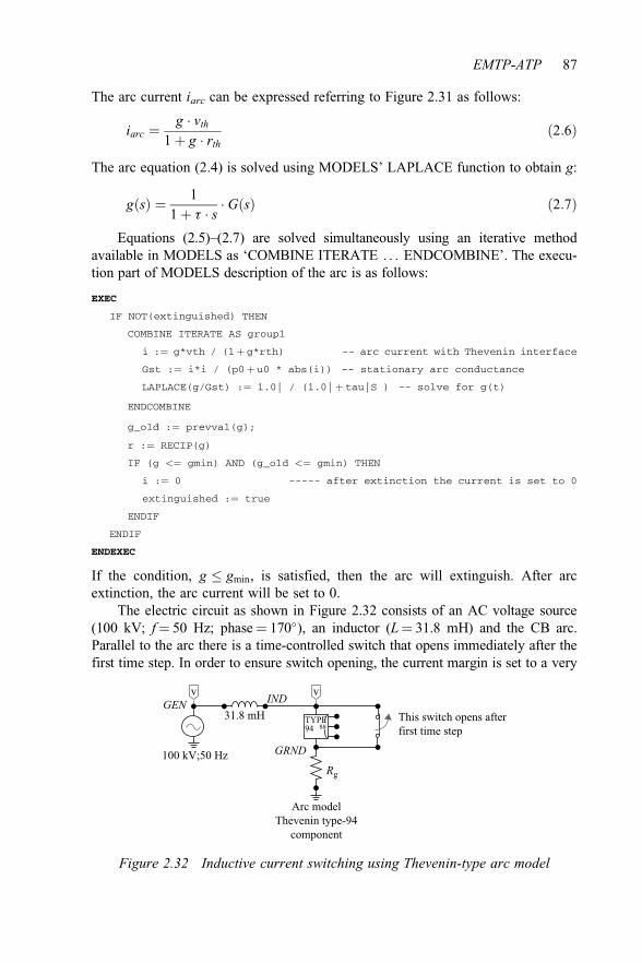
The arc current iarc can be expressed referring to Figure 2.31 as follows:

iarc ¼ g � vth

1 þ g � rthð2:6Þ

The arc equation (2.4) is solved using MODELS’ LAPLACE function to obtain g:

gðsÞ ¼ 11 þ t � s

� GðsÞ ð2:7Þ

Equations (2.5)–(2.7) are solved simultaneously using an iterative methodavailable in MODELS as ‘COMBINE ITERATE . . . ENDCOMBINE’. The execu-tion part of MODELS description of the arc is as follows:

EXEC

IF NOT(extinguished) THEN

COMBINE ITERATE AS group1

i :¼ g*vth / (1þ g*rth) -- arc current with Thevenin interface

Gst :¼ i*i / (p0þ u0 * abs(i)) -- stationary arc conductance

LAPLACE(g/Gst) :¼ 1.0| / (1.0|þ tau|S ) -- solve for g(t)

ENDCOMBINE

g_old :¼ prevval(g);

r :¼ RECIP(g)

IF (g <¼ gmin) AND (g_old <¼ gmin) THEN

i :¼ 0 ----- after extinction the current is set to 0

extinguished :¼ true

ENDIF

ENDIF

ENDEXEC

If the condition, g � gmin, is satisfied, then the arc will extinguish. After arcextinction, the arc current will be set to 0.

The electric circuit as shown in Figure 2.32 consists of an AC voltage source(100 kV; f ¼ 50 Hz; phase ¼ 170�), an inductor (L¼ 31.8 mH) and the CB arc.Parallel to the arc there is a time-controlled switch that opens immediately after thefirst time step. In order to ensure switch opening, the current margin is set to a very

100 kV;50 Hz

31.8 mH

GRND

TYPE94 ss

INDGENv v

This switch opens afterfirst time step

Arc modelThevenin type-94

component

Rg

Figure 2.32 Inductive current switching using Thevenin-type arc model

EMTP-ATP 87

high value, 100 kA. After opening of the switch the inductive current is diverted tothe electric arc. The data window of the type-94 component is shown in Figure 2.33.

The simulation results are shown in Figures 2.34 and 2.35. Contrary to thenumerical oscillations expected due to switching of an inductance, with the arcmodel no numerical oscillations occur.

2.7.4 Transformer inrush current calculationsATP supports natively the BCTRAN transformer component [3, 22] where manu-facturer’s (test report) data is used to calculate an inductance matrix transformermodel. This model does not contain support for the non-linear magnetization

Figure 2.33 Data window of the arc model

0–200

–150

–100

–50

0(kV)

50

0.1 0.2 0.3 0.4 0.5 0.6 0.7–500

500

1,000

1,500

2,000

2,500(A)

0

(ms)

Figure 2.34 Arc voltage (curve starting from 0 kV) and current (curve startingfrom 2,500 A) near current zero


characteristic, but ATPDraw offers to add this externally on one of the terminals.For inrush studies the final slope of this characteristic is of crucial importance andadding artificial points beyond the test report data is required to get correct results.Otherwise the inrush current will be substantially underestimated. Adding artificialpoint(s) is not straightforward and is most easily done in the final flux-linkage-current characteristic as shown in [30]. Another critical thing in inrush calculationsis the residual flux which to a large extent can influence the inrush current. Initi-alization of the magnetization characteristic is often difficult to achieve in practice.

ATPDraw also supports the hybrid transformer model called XFMR [23, 24].This model is based on the same type of input data as BCTRAN, but allows thecore design to be taken into account and more direct access to adding a final slopeof the magnetization characteristic. Here we bring an example from [30] thatillustrates the differences between various transformer models. The circuit diagramis shown in Figure 2.36.

Actual measurements were performed for the circuit shown in Figure 2.36. Themeasured inrush current of the target transformer is shown in Figure 2.37 and themeasured induced voltage when switching off the transformer on the 6.8 kV side isshown in Figure 2.38.

0.548–5.0

–2.5

0.0

2.5

5.0

7.5

10.0(A)

0.549 0.55 0.551 0.552 0.553 0.554 (ms) 0.5550.0

0.2

0.4

0.6

0.8

1.0(MΩ)

Figure 2.35 Arc current (thin line) and arc resistance (dark line) during arcextinction instant

3 × 550 MVA

2 × 100 Mvar

Source plant

P Q

Overhead line Targetplant

290 km 25 km

Figure 2.36 Circuit for inrush current calculations with ATP

EMTP-ATP 89

In order to evaluate the residual flux, the induced voltage on the secondary sidefor the de-energization transient prior to the inrush situation should be measuredand integrated. Capacitances in the circuit (naturally in the winding and in con-nected bushings and cables) will create a ring-down transient that will reduce the

0.46 0.48 0.5 0.52 0.54 0.56 0.58–150

–100

–50

0

50

100

Time (s)

Cur

rent

s HV

(A)

Figure 2.37 Measured inrush currents (energization), primary side

2.6 2.65 2.7 2.75–10

–5

0

5

10

Time (s)

Vol

tage

LV

(kV

)

Figure 2.38 Measured de-energization (prior to energization) transients, inducedvoltages on secondary side


residual flux. The integration of the induced voltage in Figure 2.38, shown inFigure 2.39, reveals that the residual flux here is below 10% and was ignored in thestudy [30]. Adding residual flux to the preferred inductance (pseudo-non-linear,type 98 used here) is not trivial as this device does not have a residual flux settingand that artificially application of voltage impulse is difficult in the complex net-work of inductances as seen in Figure 2.41. Jiles–Atherton non-linearities written inMODELS were instead used in [31].

2.7.4.1 Transformer modelThe transformer used in the study had an extended test report with open circuit testsup to 115% excitation and in addition information about the relative core dimen-sions and the air-core inductance were provided by the manufacturer. The hybridtransformer model XFMR was used in this study with an input dialogue shown inFigure 2.40, corresponding to the data provided in [30].

The air-core inductance calculated from the HV side consists of contributionfrom both leakage and the main flux. Ignoring the winding thickness this can bewritten

Lac ¼ La þ Lc þ LLH ¼ La þ ð1 þ kÞ � LLH ð2:8Þ

where La is the final slope of the magnetization inductance, Lc comes from theleakage channel between the inner winding and the core and LLH is the mainleakage channel. In the XFMR model Lc is estimated as LLH/2 resulting in k ¼ 0.5.

2.6 2.65 2.7 2.75–30

–20

–10

0

10

20

30

Time (s)

Flux

-link

age

LV (W

b-t)

Figure 2.39 Calculated flux-linkage by integration of the induced voltage inFigure 2.38

EMTP-ATP 91

This gives the final slope inductance

La ¼ Lac;HV � VL

VH

� �2

� ð1 þ kÞ2pf

�ffiffiffiffiffiffiffiffiffiffiffiffiffiffiffiffiffiffiffiffiffiffiffiffiffiffiffiffiffiffiffiffiffiffiffiffiffiffiffiffiffiffiffiffiffiffiffiffiffiffi

Z %½ �100

� �2

� P MW½ �S MVA½ �

� �2s

� V 2L

S

24

35 � 3

¼ 0:8289 mH ð2:9ÞThe relative core dimensions are given according to the manufacturer’s data

for the shell-form design and the core model given in Figure 2.41. Normally therelative areas are 10–15% above 1.

Figure 2.40 XFMR transformer input dialogue

CBA

Limb-AB

Out

Yok

e

Yok

e

Yok

e

Out

Leg

Leg

Leg

Limb-BC

A’B’C’

Figure 2.41 Transformer core configuration for shell-form type-B design


The final slope calculation in (2.8) can also be calculated for other transformermodels where the magnetization characteristic is connected to the artificial star pointof the transformer as in the Saturable Transformer Component (STC) or at theterminal as in BCTRAN according to [30]. This will result in characteristics as shownin Figure 2.42. As the XFMR model is based on a Frolich equation (2.3) fitting to thetest report, the final slope is added at a higher flux value compared to the BCTRANand STC models that have to use the final test report value as its second last point.

2.7.4.2 ResultsThis section compares the measured inrush currents with the calculated ones. Allmodels give fairly good agreement, but the XFMR with the detailed core infor-mation (shell-form) manages to reproduce most of the details better. The reason forthe fairly well agreement in all models is that the test report goes up to 115%excitation with additional air-core information (Figure 2.43).

2.7.5 Power system toolbox: relayingATPDraw offers a power system toolbox with calculation of steady-state qualitiesand relay protection devices. The work horse of this toolbox is the DFT algorithmthat is used for the phasor calculations. The components in the toolbox have anopen source so that users can modify and add sophistication.

2.7.5.1 Phasor calculationsThe work horse of the toolbox is a DFT algorithm in MODELS that calculatesthe fundamental (and harmonic) component of the time-domain signal by a

0 1 2 3 4 5 6 70.6

0.7

0.8

0.9

1

1.1

1.2

1.3

Current peak (%)

Flux

link

age

(pu)

XFMR shell (leg)

XFMR shell (yoke)

XFMR shell (m&o limb)

XFMR triplex

BCTRAN & STC

Figure 2.42 Magnetization characteristics of the transformer models, based ontest report and extra final slope

EMTP-ATP 93

moving window. The algorithm takes advantage of several of the signal proces-sing specialities of the MODELS language as shown in the programs below.

Sample frequency control is added with the declaration timestep min:1/SampleFreq, which simply puts an upper constraint of the local timestep in the model and where SampleFreq is given in Samples/second.

Low-pass filtering is added with the line claplace(Y[i]/X[i]):¼(1|s0)/(1|s0þtau|s1), where X is the input signal and Y is thefiltered signal that is used further in the DFT calculations and where tau isdefined as tau:¼recip(2*PI*FilterFreq). recip is a 1/x functionwith zero division protection. The claplace function uses the |s0 and |s1operators to define the transfer function.

Calculation of phasors is done with the syntax

D:¼1/PI*((f4-f2)*sin(OMEGA*T)-(f3-f1)*sin(OMEGA*(T-timestep))

þ(f4-f3-f2þf1)/(timestep*OMEGA)*(cos(OMEGA*T)-cos(OMEGA*(T-time-

step)))),

where D is the incremental contribution to the Fourier coefficients in which a fewdelay functions are used to throw out the sample one period ago and add the mostrecent sample.

The algorithm is based on assuming a linear behaviour of the signal y(t)between two sample points so that it can be written yðtÞ ¼ ai � t þ bi ^ t

0.46 0.48 0.5 0.52 0.54 0.56–150

–100

–50

0

50

100

(a) (b)

(c) (d)

150

Time (s)

Cur

rent

HV

(A)

0.46 0.48 0.5 0.52 0.54 0.56–150

–100

–50

0

50

100

150

Time (s)

Cur

rent

HV

(A)

0.46 0.48 0.5 0.52 0.54 0.56–150

–100

–50

0

50

100

Time (s)

Cur

rent

HV

(A)

0.46 0.48 0.5 0.52 0.54 0.56–150

–100

–50

0

50

100

Time (s)

Cur

rent

HV

(A)

Figure 2.43 (a) STC; (b) BCTRAN; (c) XFMR (shell B); (d) XFMR (triplex)


2 i � Dt; ði þ 1Þ � Dt½ � which is the same assumption as used in the trapezoidal ruleof integration. The Fourier series coefficients can then be written

ahðtÞ ¼ wp

ðtt�T

yðtÞ � cosðhw � tÞ � dt � wp

Xm

i¼0

ðt�Tþðiþ1ÞDt

t�Tþi�Dt

ai � tþ bið Þ�cosðhw � tÞ � dt

¼ 1h � p

Xm

i¼0

ai

hwcosðhwðt þ ði þ 1ÞDtÞÞ � cosðhwðt þ iDtÞÞð Þ

�

þðaiDt þ biÞ � sinðhwðt þ ði þ 1ÞDtÞÞ � sinðhwðt þ iDtÞÞð Þ�

ð2:10ÞSimilarly bhðtÞ ¼ w

p

Ð tt�T yðtÞ � sinðhw � tÞ � dt, where T is the period, h is the har-

monic number, w is the angular frequency and m ¼ T=Dt þ 1.By assuming a moving window of one period, the increment of the

Fourier coefficients can be written DahðtÞ ¼ ahðt; i ¼ mÞ � ahðt; i ¼ �1Þ andDbhðtÞ ¼ bhðt; i ¼ mÞ � bhðt; i ¼ �1Þ which is exactly what is calculated by theMODELS code below:

MODEL ABC2PHR2

INPUT X[1..3] --input signal to be transformed

DATA FREQ {dflt:50} --power frequency

SCALE {dflt:1} --multiply output by this number

FilterFreq {dflt:400}--low-pass corner frequency

SampleFreq {dflt:800}--actual sample frequency of algorithm

OUTPUT reF[1..3], imF[1..3] –DFT signals

VAR reF[1..3], imF[1..3], NSAMPL, OMEGA, Y[1..3]

D,F1,F2,F3,F4,i, h, tau, timestep min:1/SampleFreq

HISTORY Y[1..3] {dflt:0}

DELAY CELLS (Y[1..3]) : 1/(FREQ*timestep)þ1

INIT

OMEGA:¼ 2*PI*FREQ

NSAMPL:¼recip(FREQ*timestep)

tau:¼recip(2*PI*FilterFreq)

reF[1..3] :¼0

imF[1..3] :¼0

h:¼1 --harmonic number

ENDINIT

EXEC

FOR i:¼1 TO 3 DO

claplace(Y[i]/X[i]):¼(1|s0)/(1|s0þtau|s1)

f1:¼delay(Y[i],(NSAMPLþ1)*timestep,1)

f2:¼delay(Y[i],NSAMPL*timestep,1)

f3:¼delay(Y[i],timestep,1)

f4:¼Y[i]

D:¼1/(h*PI)*((f4-f2)*sin(h*OMEGA*T)-(f3-f1)*sin(h*OMEGA*(T-timestep))

EMTP-ATP 95

þ(f4-f3-f2þf1)/(timestep*h*OMEGA)*

(cos(h*OMEGA*T)-cos(h*OMEGA*(T-timestep))))

reFh[i]:¼reFh[i]þD*scale

D:¼1/(h*PI)*((f4-f2)*cos(h*OMEGA*T)-(f3-f1)*cos(h*OMEGA*(T-timestep))

-(f4-f3-f2þf1)/(timestep*h*OMEGA)*

(sin(h*OMEGA*T)-sin(h*OMEGA*(T-timestep))))

imFh[i]:¼imFh[i]þD*scale

ENDFOR

ENDEXEC

ENDMODEL

2.7.5.2 Power and impedance calculationsThe algorithm shown in the program above is used also for PQ and RX calculationsand in that case the phasors of two three-phase input current I [1..3] and voltageV [1..3] are calculated. This gives

R þ jX ¼ Vre þ jVim

Ire þ jIimand P þ jQ ¼ Vre þ jVimð Þ � Ire � jIimð Þ ð2:11Þ

For distance relays the positive-sequence impedance is needed and this is found bycalculating line quantities as shown below for the (real part of the) voltage:

VL[n]:¼(V[n]-V[(n mod 3) þ1])

claplace(YV[n]/VL[n]):¼(1|s0)/(1|s0þtau|s1)

2.7.5.3 Relay functionalityAll the relays connect to a signal conditioning model (rms value, RX calculation,phasor calculation). They have further a block-signal input, a diagnosis output anda trip signal. All relays have also a zone and trajectory plot functionality. This isaccomplished by reading in data from the LIS file.

● The overcurrent relay has either a constant or inverse time characteristic. Inboth the cases, the rms value of the current is used as input.

● The distance relay uses an RX input and contains settings for three zones withquadrilateral characteristic.

● The differential relay contains also harmonic blocking functionality. Theh-harmonic of the signal can easily be obtained from the above programs bysetting h to typically 2 or 5 and use a criterion for how much harmonic isallowed before trip should be blocked.

2.7.5.4 ExampleThe example illustrates a two-phase fault in a 420 kV system and the response of adistance relay. The circuit is shown in Figure 2.44 and consists of three 420 kVtransmission lines in a meshed network, one source and two loads at the secondaryside of 420:132 kV transformers. A distance relay is located as BUS1 looking intothe line to BUS2. A phase-to-phase fault is applied at BUS2.


The transmission line modelling is equivalent to what is described in section2.7.1, Figure 2.22, but the sky-wires are now assumed at ground potential by settingtheir Ph. No ¼ 0 in Figure 2.23. The line is still modelled as a JMarti line even if asimple PI equivalent could have been sufficient.

The transformers are modelled with the BCTRAN component with simple andtypical data input. The data are similar to those in Figure 2.40, but simplifiedsomewhat as saturation is not important here as shown in Figure 2.45.

The distance relay at BUS1 gets its RX signals from a DFT algorithm in apredefined MODELS component UI2RXL (line quantities) with a low-pass filterand sample frequency restrictions added as described above. The model has theinput data as shown in Figure 2.46.

The UI2RXL model must be written to the ATP file prior to the relay modeland to enforce this, the Order option can be used. The relay model has the inputdata as shown in Figure 2.47. This consists of the time delay for each of the threezones, four RX points for each of the three zones, an RL-XL point describing theline (just for plotting), a DownSample setting to reduce printout, a t_init setting thatdescribes the minimum time for the relay to respond (typically one period requiredto get reliable DFT signals) and an Idx value to identify the relay if several valuesare used in the data case.

2.7.5.5 ResultThe trajectory of all the relay can be plotted related to their zones of protection asseen in Figure 2.48. This shows initially the load position as seen from the relay

BUS1BUS2

BUS3

420:132 kV

100 MW

420:132 kV

Phase-to-phase fault

10+j25 MVA

Y YY

LCC

100. km LCC

50. km100. km

Phase faultsDistance relay

B T ?

21

M

V Δ

Δ Y

Δ Y

Δ

M

ui

RX

LCC

Template

LCC

Figure 2.44 Distance relay example circuit

EMTP-ATP 97

Figure 2.45 Transformer model as BCTRAN component

Figure 2.46 Input data to RX-calculation module UI2RXL

Figure 2.47 Input data to distance relay module W1RELAY21P, three zones,four points per zone


towards the steady-state fault location. In this case the phase A trajectory (thatcorresponds to phase A-B faults) will enter the trip zones around the boundary ofzone 2. Zone 2 should thus have been extended in X-direction to better cover thisfault.

References

[1] Dommel H. W., ‘Digital computer solution of electromagnetic transients insingle and multiphase networks,’ IEEE Transactions on Power Apparatusand Systems, vol. PAS-88, April 1969, pp. 388–399.

[2] Meyer W. S., Dommel H. W., ‘Numerical modelling of frequency-dependenttransmission-line parameters in an electromagnetic transients program’,IEEE Transactions on Power Apparatus and Systems, vol. PAS-93, no. 5,1974, pp. 1401–1409.

[3] Bonneville Power Administration. EMTP Theory Book, Branch of SystemEngineering, Oregon, USA, 1987 Available from the secure EEUG websitehttp://www.eeug.org.

[4] Canadian/American EMTP User Group. ATP Rule Book, Portland, Oregon,USA, revised and distributed by the EEUG Association, 2014. Availablefrom the secure EEUG website http://www.eeug.org.

[5] Dube L., Bonfanti, I., ‘MODELS: A new simulation tool in the EMTP’,European Transactions on Electrical Power, vol. 2, no. 1, January/February1992, pp. 45–50.

[6] Dube L., Dommel H. W., ‘Simulation of control systems in an electro-magnetic transients program with TACS’, Proceedings of the IEEE PICAConference, May 1972, pp. 266–271.

[7] Furst G., Kizilcay M., ‘Frequency-domain harmonic analysis using the ATP-EMTP program’, International Conference on Electrical Engineering 2000(ICEE), IEE Japan, Kitakyushu, Japan, July 24–28, 2000.

–0.5–1.5

–1.0

–0.5

0.0

0.5

1.0

1.5

2.0

0.0 0.5R (kohms)

X (k

ohm

s)

X (o

hms)

1.0 1.5 2.0 –100–100

–50

50

100

0

–50 0 50 100R (kohms)

Figure 2.48 Distance relay example with trajectory plots

EMTP-ATP 99

[8] CIGRE Working Group 36-05. ‘Harmonics, characteristic parameters,methods of study, estimates of existing values in the network’, Electra,vol. 77, 1981, pp. 35–54.

[9] Mohan N., Computer Exercises for Power Electronic Education, Depart-ment of Electrical Engineering, University of Minnesota, Minneapolis, MN,1990.

[10] Semlyen A., Dabuleanu A., ‘Fast and accurate switching transient calcula-tions on transmission lines with ground return using recursive convolutions’,IEEE Transactions on Power Apparatus and Systems, vol. PAS-94, no. 2,1975, pp. 561–571.

[11] Marti J. R., The Problem of Frequency Dependence in Transmission LineModelling, Ph.D. dissertation, University of British Columbia, Canada,1981.

[12] Marti J. R., ‘Accurate modelling of frequency-dependent transmission linesin electromagnetic transient simulations’, IEEE Transactions on PowerApparatus and Systems, vol. PAS-101, no. 1, 1982, pp. 147–155.

[13] Noda T., Nagaoka N., Ametani A., ‘Phase domain modeling of frequency-dependent transmission lines by means of an ARMA model’, IEEE Transactionson Power Delivery, vol. 11, no. 1, January 1996, pp. 401–411.

[14] Noda T., Nagaoka N., Ametani A., ‘Further improvements to a phase-domainARMA line model in terms of convolution, steady-state initialization, andstability’, IEEE Transactions on Power Delivery, vol. 12, no. 3, July 1997,pp. 1327–1334.

[15] Gross G., Hall M. C., ‘Synchronous machine and torsional dynamics simu-lation in the computation of electromagnetic transients’, IEEE Transactionson Power Apparatus and Systems, vol. PAS-97, no. 4, 1978, pp. 1074–1086.

[16] Brandwajn V., Dommel H. W., ‘A new method for interfacing generatormodels with an electromagnetic transients program,’ IEEE PES PICA Con-ference Record, May 24–27, 1977, pp. 260–265.

[17] Lauw H. K., Meyer W. S., ‘Universal machine modeling for the representationof rotating electric machinery in an electromagnetic transients program’,IEEE Transactions on Power Apparatus and Systems, vol. 101, no. 6, 1982,pp. 1342–1351.

[18] Prikler L., Høidalen H. K., ATPDraw for Windows 3.1x/95/NT version 1.0 –User’s Manual, 1998. Available from http://www.atpdraw.net.

[19] Prikler L., Høidalen H. K., ATPDRAW version 3.5 for Windows 9x/NT/2000/XP, 2002. Available from http://www.atpdraw.net.

[20] Prikler L., Høidalen H. K., ATPDRAW version 5.6 for Windows 9x/NT/2000/XP/Vista, 2009. Available from http://www.atpdraw.net.

[21] Høidalen H. K., Mork B. A., Prikler L., Hall J. L., ‘Implementation of newfeatures in ATPDraw version 3’, Proceedings of the International Conferenceon Power System Transients (IPST), New Orleans, LA, 29 Sep–2 Oct 2003.

[22] Brandwajn V., Dommel H. W., Dommel I. I., ‘Matrix representation of three-phase N-winding transformers for steady-state and transient studies’, IEEE


Transactions on Power Apparatus and Systems, vol. PAS-101, no. 6, 1982,pp. 1369–1378.

[23] Høidalen H. K., Mork B. A., Gonzalez F., Ishchenko D., Chiesa N.,‘Implementation and verification of the hybrid transformer model in ATP-Draw’, Proceedings of the International Conference on Power SystemTransients (IPST), Lyon, France, 3–7 June 2007.

[24] Høidalen H. K., Chiesa N., Avendano A., Mork B. A., ‘Developments in thehybrid transformer model – Core modeling and optimization’, Proceedingsof the International Conference on Power System Transients (IPST), Delft,the Netherlands, 14–17 June 2011.

[25] Høidalen H. K., ‘Universal machine modeling in ATPDraw – EmbeddedWindsyn’, Proceedings of the EMTP-ATP Users Group meeting, Ohrid,Makedonia, 25–28 September 2011.

[26] Ceraolo M., ‘PlotXY – a new plotting program for ATP’, EEUG News,February–May 1998. Available from http://www.eeug.org.

[27] Martinez-Velasco J. A. (Ed.), Power System Transients – ParameterDetermination, CRC Press, New York, 2010.

[28] Høidalen H. K., Radu D., Penkov D., ‘Optimization of cost functions inATPDraw’, Proceedings of the EMTP-ATP Users Group meeting, Delft, theNetherlands, 26–27 October 2009.

[29] Grutz A., Hochrainer A., ‘Rechnerische Untersuchung von Leistungsschalternmit Hilfe einer verallgemeinerten Lichtbogentheorie’, etz-a, vol. 92, no. 4,1971, pp. 185–191 (in German).

[30] Chiesa N., Høidalen H. K., Lambert M., Duro M. M., ‘Calculation of inrushcurrents – benchmarking of transformer models’, Proceedings of the Interna-tional Conference on Power System Transients (IPST), Delft, the Netherlands,14–17 June 2011.

[31] Chiesa N., Mork B. A., Høidalen H. K., ‘Transformer model for inrushcalculations: simulation, measurements and sensitivity analysis’, IEEETransactions on Power Delivery, vol. 25, no. 4, 2010, pp. 2599–2608.

EMTP-ATP 101

Chapter 3

Simulation of electromagnetic transientswith EMTP-RV

J. Mahseredjian*, Ulas Karaagac*, Sebastien Dennetiere†

and Hani Saad†

3.1 Introduction

EMTP-RV is the restructured version of the Electromagnetic Transients Program(EMTP). It is a simulation tool for electromagnetic transients (EMTs) in powersystems. The development of EMTP-RV was initiated and completed in the Devel-opment Coordination Group (DCG) of EMTP. It was funded by several internationalorganizations. The objective of the development of EMTP-RV, RV standing forrestructured version, was to rewrite and modernize the EMTP code using the latestprogramming techniques, and the most recent research on models and solutionmethods in the field of power system transients. The overall programming effortstarted in 1998 and was completed in 2003. Due to technical reasons, it was decidedto abandon completely the old DCG-EMTP code and program EMTP-RV fromscratch; that is why EMTP-RV does not contain any computer code lines from theold DCG-EMTP and innovates in several aspects as described below.

EMTP-RV is a commercial software package [1] used by many universitiesand industrial organizations worldwide.

Since the letters RV are only used to denote the new generation of EMTP, theyare dropped in the following sections by using only the software acronym EMTP.

3.2 The main modules of EMTP

The main modules of EMTP, presented in Figure 3.1, are:

1. Graphical user interface (GUI)2. Data input file3. Multiphase load-flow solution4. Steady-state solution5. Initialization: automatic or manual initial conditions

*Ecole Polytechnique de Montreal, Canada†RTE, France

6. Time-domain solution7. Results: waveforms and outputs8. External programming interface

The main modules are described in the following sections.

3.3 Graphical user interface

The graphical user interface (GUI) is the first entry level to the simulation processof EMTP. It is the simulated network schematic input. An example of EMTPschematic input is presented in Figure 3.2. The EMTP GUI is called EMTPWorks.

The EMTP GUI is based on a hierarchical design approach with subnetworksand masking. Subnetworks allow simplifying the drawing and hiding details whilemasking provides data encapsulation. The design of Figure 3.2 uses several sub-networks. The 230 kV network is interconnected with a 500 kV network evacuatedwith all its details into the subnetwork shown in Figure 3.2. In a hierarchical design,subnetworks can also contain other subnetworks. Subnetworks can be also used todevelop models. The three-phase transformers shown in Figure 3.2 are based on theinterconnection of single-phase units. The synchronous machine subnetworkscontain load-flow constraints, machine data and subnetworks with voltage reg-ulator and governor controls, as shown in Figure 3.2.

The EMTP GUI is programmed using three layers (Figure 3.3). The first layeris the hard code of the software (written in C/Cþþ) containing all its operations,menus, drawing tools and manipulations of data. The second layer delivers inter-facing methods for full access to schematic drawing functions and data scripting.This layer is based on JavaScript with extensions for EMTPWorks and constitutes

Multiphase load-flow

Steady state

Time domain

Initialization

Graphical user interface (GUI)

Results

Data

External programminginterface

Figure 3.1 EMTP computation modules


SM4

BU

S4

DY

g_B

US4

BU

S5

BU

S1

Subo

fBU

S1

+12

0kTL

M_1

20m

i

BU

S12 Y

gD_B

US1

3BU

S13

56MW12MVAR

57MW16MVAR

60MW16MVAR

120m

0.99

/_20

.7B

US2

BU

S11

13.8

/230

69/2

30

SM SM11

BU

S218

0m

500

kV

N S

CP

SUB

_BU

S1

45M

W21

MV

AR

LF

0.99

/_56

.5

BU

S7

CP

TLM

_90m

i

BU

S10.

99/_

40.3

BU

S6

BU

S6PV

bus:

SM_B

US6

AV

R_G

ov

Out IN

AV

R&

Gov

(pu)

LF

SM SMSM8

BU

S8D

Yg_

BU

S8

13.8

/230

0.96

/_43

.7

BU

S9 180k

Load9

LF24

0MW

60M

VA

R

TLM

_180

mi

Load

13c

Load

13b

Load

13a

CP2

13.8

kV55

0MV

A

P=52

0MW

V=1

3.8k

VR

MSL

LSM

:SM

6

DY

g_B

US6

13.8

/230 0.

99/_

56.0

+

+

+TL

M_1

5mi

CP

LFc

b

a

LF

LF

+

SM6

SM

TLM_10miTLM_60miCP

CP

+ untra

nspo

sed

untra

nspo

sed

Load5

12

13.8

/230

SM

12

12

12

12

Fig

ure

3.2

Sam

ple

230

kVne

twor

ksi

mul

atio

npr

esen

ted

ina

GU

I

the interface for the third layer. It provides a large collection of functions, allowingthe software developers and users to program data input panels and symbols forEMTP models. EMTPWorks data input functions are based on dynamic HTML(DHTML). A large collection of JavaScript functions also allows the writing ofscripts for externally modifying data and restarting simulations. Interfacing withActiveX and all types of application programming interfaces is also possiblethrough the JavaScript layer.

3.4 Formulation of EMTP network equations for steady-stateand time-domain solutions

The objective of this section is to present a brief overview on the numericalmethods used in EMTP.

Bold characters are used hereafter for the representation of vectors and matrices.

3.4.1 Modified-augmented-nodal-analysis used in EMTPThe traditional approach for the formulation of main network equation is based onnodal analysis. The network admittance matrix Yn is used for computing the sum ofcurrents entering each electrical node and the following equation results fromclassical nodal analysis.

Yn vn ¼ in ð3:1Þwhere vn is the vector of node voltages and the members of in hold the sum ofcurrents entering each node. It is assumed that the network has a ground node atzero voltage which is not included in (3.1). Since the network may contain voltagesources (known node voltages), (3.1) must be normally partitioned to keep only theunknown voltages on the left-hand side:

Y0n v0n ¼ i0n � Ys vs ð3:2Þ

where Y0n is the coefficient matrix of unknown node voltages v0n, i0n holds the sum

of currents entering nodes with unknown voltages, Ys 2 Yn and relates to knownvoltages vs. It is noticed that vn ¼ v0

n vs½ �T .

C/C++

Interfacemethods JavaScript

DHTML

Figure 3.3 EMTPWorks layers


Equation (3.1) has several limitations. It does not allow, for example, the modelingof branch relations instead of nodal relations and it basically assumes that everynetwork model has an admittance matrix representation, which is not possible in manycases. That is why EMTP uses the modified-augmented-nodal analysis (MANA) [2–4]formulation. Equation (3.1) is augmented to include generic device equations and thecomplete system of network equations can be rewritten in the more generic form:

AN xN ¼ bN ð3:3ÞIn this equation Yn 2 AN, xN contains both unknown voltage and current quantitiesand bN contains known current and voltage quantities. The matrix AN is notnecessarily symmetric in EMTP and it is possible to directly accommodate non-symmetric model equations. Equation (3.3) can be written explicitly as

Yn Ac

Ar Ad

� �vn

ix

� �¼ in

vx

� �ð3:4Þ

where the matrices Ar, Ac, and Ad (augmented portion, row, column, and diagonalcoefficients) are used to enter network model equations which are not or cannot beincluded in Yn; ix is the vector of unknown currents in device models, vx is thevector of known voltages, xN ¼ vn ix½ �T and bN ¼ in vx½ �T . In reality the net-work component equations can be entered in any order in (3.3), but the partitioningpresented in (3.4) allows to simplify explanations. Further details can be found in[3] and [4].

Equation (3.3) (or (3.4)) can be used for both steady-state and time-domainsolutions. A generic coupled admittance model is written as

ikim

� �¼ Ykk Ykm

Ymk Ymm

� �vk

vm

� �ð3:5Þ

where ik and im represent the current vectors for the sum of currents entering the kside and m side nodes, respectively, the vectors vk and vm represent the voltages onthe k side and m side nodes, respectively. In most cases Ykm ¼ Ymk and theresulting matrix Yn is symmetric, but EMTP also allows to use Ykm 6¼ Ymk.

For the case of a generic model equation such as

k1vk þ k2vm þ k3ix þ k4iy þ � � � ¼ bz ð3:6Þwhere the unknown node voltages (vk ,vm) and branch currents (ik ,im) are membersof xN, while bz is entered into bN. Any number of unknown node voltages andbranch currents can be used and (3.6) can also include coupling by rewriting it withvectors and matrices. A three-phase voltage source, for example, connected betweentwo arbitrary nodes k and m is expressed as:

vk � vm � Zsikm ¼ vb km ð3:7Þwhere Zs is the source impedance, ikm 2 ix representing source currents (enteringplus node k) and vb km 2 vx is the known source voltage. This equation contributes

Simulation of electromagnetic transients with EMTP-RV 107

its own row into Ar with coefficients 1 and �1 on the columns k and m, respectively.The impedance Zs (can be set to zero) is entered into a diagonal block of Ad. Therow contributed into Ar is transposed and placed into the corresponding column ofAc. Equation (3.7) can be rewritten in its single-phase form using scalars.

For a single-phase ideal switch model there are two states. In the closed state:

vk � vm ¼ 0 ð3:8Þand in the open state:

ikm ¼ 0 ð3:9Þwhere ikm is the switch current entering node k and leaving node m. Equation (3.8)is entered into (3.4) by setting:

Arik ¼ 1; Arim ¼ �1Acki ¼ 1; Acmi ¼ �1Adii ¼ 0

ð3:10Þ

where Ar 2 Ar, Ac 2 Ac, Ad 2 Ad and the switch equations are entered into the ithrow. In the case of (3.9), the formulation becomes:

Arik ¼ 0; Arim ¼ 0Acki ¼ 1; Acmi ¼ �1Adii ¼ 1

ð3:11Þ

Equation (3.11) makes AN non-symmetric and it is also noticed that any switchstatus change requires updating AN. It is also possible to model a non-ideal switchusing:

vk � vm � RS ikm ¼ 0 ð3:12Þwith RS being the switch resistance. In this case, the contributions into AN become:

Arik ¼ 1; Arim ¼ �1Acki ¼ 1; Acmi ¼ �1Adii ¼ �RS

ð3:13Þ

The resistance RS is replaced by a very high value for the switch open state andby a very low value for the switch closed state. In the closed state, it is allowed tomake RS ¼ 0 to obtain the ideal condition.

Single-phase and three-phase transformers can be built in EMTP using theideal transformer unit shown in Figure 3.4. It consists of dependent voltage andcurrent sources. The secondary branch equation is given by

vk2 � vm2 � g vk1 þ g vm1 ¼ 0 ð3:14Þwhere g is the transformation ratio. This equation contributes its own row into thematrix Ar, whereas the matrix Ac contains the transposed version of that row. It ispossible to extend to multiple secondary windings using parallel connected current


sources on the primary side and series connected voltage sources on the secondaryside. Leakage losses and the magnetization branch are added externally to this idealtransformer nodes.

Three-legged core-form transformer models or any other types can be includedusing coupled leakage matrices and magnetization branches.

The MANA formulation (3.3) of EMTP is completely generic and can easilyaccommodate the juxtaposition of arbitrary component models in arbitrary networktopologies with any number of wires and nodes. It is not limited to the usage of theunknown variables presented in (3.4) and can be augmented to include differenttypes of unknown and known variables. The MANA formulation is conceptuallysimple to realize and program.

3.4.1.1 Steady-state solutionThe steady-state version of (3.3) is based on complex numbers. Equation (3.3) isrewritten using capital letters for the specific case of complex variables (phasors).

AN XN ¼ BN ð3:15ÞFor a network containing sources with different frequencies, (3.15) can be

independently solved at each frequency and, assuming that the network is linear(linear models are used for all devices), the solutions of XN at each frequency arecombined to derive the harmonic steady-state solution in the form of a Fourierseries. EMTP is able to produce a steady-state linear harmonic solution.

In EMTP the steady-state solution is calculated for the frequencies of thestudied network, but can be also calculated for a user-specified frequency rangefor performing frequency scans. The frequency scan option can be also used tocalculate Thevenin impedances at arbitrary locations in the network. Sequenceimpedances can be calculated from three-phase buses.

3.4.1.2 Time-domain solutionEMTP uses the trapezoidal integration method with Backward Euler for the treat-ment of discontinuities. This approach is similar to [5, 6].

k1

–g ik2m2 g (vk1 – vm1)

ik2m2

m1

k2

+

–

m2

Figure 3.4 Ideal transformer model unit


For an ordinary differential equation given by

dx

dt¼ f ðx; tÞ

xð0Þ ¼ x0

ð3:16Þ

the trapezoidal integration rule allows to write:

xt ¼ Dt

2ft þ Dt

2ft�Dt þ xt�Dt ð3:17Þ

The time-domain module of EMTP starts from 0-state (all devices are initiallydeenergized) or from given automatic or manual initial conditions and computes allvariables as a function of time using a time-step Dt. The terms found at t � Dtconstitute history terms and all quantities at time-point t are also related throughnetwork equations. The computation process finds a solution at discrete time-pointsas illustrated in Figure 3.5.

During a discontinuity, (3.17) may cause numerical oscillations. Such oscil-lations can be eliminated by moving into two halved time-step integrations usingthe Backward Euler method. In this case, (3.17) becomes:

xt ¼ Dt

2ft þ xt�Dt

2ð3:18Þ

where t � Dt=2 is the discontinuity detection time-point. After the completion ofhalved time-step solutions with (3.18), and if there are no other discontinuities, thesolution method moves back to (3.17). Discontinuities can be automaticallydetected, for example, from ideal switches changing states, sources starting andstopping and nonlinear functions changing slopes. They become more complicatedto detect with black-box type device models and generic nonlinear functions.Although the concept of this approach is relatively simple, its actual implementa-tion causes several complexities and specific equations must be derived for eachdevice model in EMTP.

0

With initialconditions

No initialconditions

Δt 2Δt 3Δt 4Δtt

x

Figure 3.5 Discrete solution time-points


In the time-domain solution, EMTP uses the real version of (3.3) for solvingthe algebraic-differential equations of the network. At each solution time-point:

ANt xNt ¼ bNt ð3:19ÞThis is achieved simply by converting or discretizing the device equations

using a numerical integration technique such as (3.17). For a pure inductor branchconnected between two nodes k and m:

vkm ¼ Ldikm

dtð3:20Þ

and the discretized version (equivalent circuit model or companion branch) [7–9] isgiven by

it ¼ Dt

2Lvt þ Dt

2Lvt�Dt þ it�Dt ð3:21Þ

where the km subscript is dropped to simplify notation. Since the last two terms ofthis equation represent computations available from a previous time-point solution,it can be written as

it ¼ Dt

2Lvt þ iht ð3:22Þ

where iht is a history term for the solution at the time-point t. The history termcontributes into bNt , the coefficient of voltage contributes into ANt and vt 2 xNt .More specifically, (3.22) is rewritten as follows at the time-point t:

ik

im

� �¼ y �y

�y y

� �vk

vm

� �þ ih

�ih

� �ð3:23Þ

where y ¼ Dt2L.

An equation similar to (3.22) is written for capacitor branches. The inductor,capacitor, and resistor are primitive elements for building other models.

The companion branch approach is generalized in EMTP to include coupledbranch models, rotating machines, and other components with differential equa-tions. The generic nodal admittance formulation is similar to (3.5), but since it isdone in time-domain, it includes history terms as in (3.23).

3.4.1.3 Nonlinear modelsNonlinearities occur due to nonlinear functions used in EMTP network devicemodels. In most cases a nonlinear function can be modeled using piecewise linearsegments. The positive part of a sample nonlinear function with 3 segments isshown in Figure 3.6 for a voltage vx tð Þ and a current ix tð Þ. In EMTP such functionsare monotonically increasing since it is assumed that there is a unique solution for agiven voltage. Each segment j is represented by a liner equation:

ixj ¼ Kj vxj þ iqj ð3:24Þ


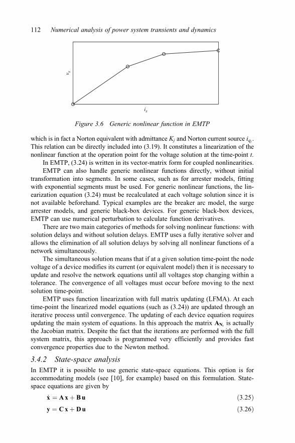
which is in fact a Norton equivalent with admittance Kj and Norton current source iqj .This relation can be directly included into (3.19). It constitutes a linearization of thenonlinear function at the operation point for the voltage solution at the time-point t.

In EMTP, (3.24) is written in its vector-matrix form for coupled nonlinearities.EMTP can also handle generic nonlinear functions directly, without initial

transformation into segments. In some cases, such as for arrester models, fittingwith exponential segments must be used. For generic nonlinear functions, the lin-earization equation (3.24) must be recalculated at each voltage solution since it isnot available beforehand. Typical examples are the breaker arc model, the surgearrester models, and generic black-box devices. For generic black-box devices,EMTP can use numerical perturbation to calculate function derivatives.

There are two main categories of methods for solving nonlinear functions: withsolution delays and without solution delays. EMTP uses a fully iterative solver andallows the elimination of all solution delays by solving all nonlinear functions of anetwork simultaneously.

The simultaneous solution means that if at a given solution time-point the nodevoltage of a device modifies its current (or equivalent model) then it is necessary toupdate and resolve the network equations until all voltages stop changing within atolerance. The convergence of all voltages must occur before moving to the nextsolution time-point.

EMTP uses function linearization with full matrix updating (LFMA). At eachtime-point the linearized model equations (such as (3.24)) are updated through aniterative process until convergence. The updating of each device equation requiresupdating the main system of equations. In this approach the matrix ANt is actuallythe Jacobian matrix. Despite the fact that the iterations are performed with the fullsystem matrix, this approach is programmed very efficiently and provides fastconvergence properties due to the Newton method.

3.4.2 State-space analysisIn EMTP it is possible to use generic state-space equations. This option is foraccommodating models (see [10], for example) based on this formulation. State-space equations are given by

_x ¼ A x þ B u ð3:25Þy ¼ C x þ D u ð3:26Þ

ix

v x

Figure 3.6 Generic nonlinear function in EMTP


where x is the vector of state variables, u is the vector of inputs and y is the vectorof outputs. The matrices A, B, C, and D are called the state matrices. Thesematrices can be calculated for given ideal switch positions and piecewise lineardevice segments. Each topological change requires updating the state matrices.EMTP allows to use the more generic version:

y ¼ C x þ D u þ D1 _u ð3:27Þfor output equations.

The state-space equations (3.25) and (3.26) can be solved in both steady-stateand time-domain. Other theoretical details can be found in EMTP documentationand [11].

3.4.2.1 Steady-state solutionIn steady-state conditions the differential of x is transformed into s~X with theLaplace operator s ¼ jw (w is the steady-state frequency in rad/s and j is thecomplex operator):

~X ¼ s I � Að Þ�1 B ~UÞ� ð3:28Þwhere tilde-upper-case vectors are used to denote phasors and I is the identitymatrix. Equation (3.27) can be written in steady-state as

~Y ¼ C s I � Að Þ�1 B þ D þ s D1

h i~U ð3:29Þ

In this equation ~U represents network voltages and ~Y corresponds to currents.This means that (3.29) has the same shape as (3.5) and can be directly enteredinto (3.15).

3.4.2.2 Time-domain solutionIn time-domain the state-space equations are discretized using trapezoidal integra-tion and Backward Euler for discontinuities. It can be shown that (3.25) results into

xt ¼ I � Dt

2A

� ��1

I þ Dt

2A

� �xt�Dt þ I � Dt

2A

� ��1 Dt

2B ut þ ut�Dtð Þ ð3:30Þ

when discretized through the trapezoidal integration method of (3.17). Equation(3.30) can be written as

xt ¼ A xt�Dt þ B ut�Dt þ B ut ð3:31Þwhere hatted matrices result from the discretization process.

Once (3.25) and (3.27) (or (3.26)) are defined for a given model (or group),they can be inserted into the main network equation (3.19) and simultaneouslyinterfaced with other model equations based on state-space or nodal formulations.It is first noticed that (3.27) can be rewritten at a solution time-point t in terms ofcurrent injections it and nodal voltages vt:

it ¼ Ck xt þ Dk vt þ ict ð3:32Þ


where trapezoidal integration for the capacitive current (ict ) results into

ict ¼2Dt

D1k vt � 2Dt

D1k vt�Dt � ict�Dt ð3:33Þ

The state equations are now written with input voltage:

xt ¼ Ak xt�Dt þ Bk vt�Dt þ Bk vt ð3:34ÞEquations (3.33) and (3.34) can be replaced into (3.32) for creating a nodal for-mulation that can be directly integrated into (3.19).

3.5 Control systems

The simulation of control system dynamics is fundamental for studying power sys-tem transients. In EMTP, control elements can be transfer functions, limiters, gains,summers, integrators, and many other mathematical functions. In many applicationsthe block-diagram approach is used in EMTP to build and interface user-definedmodels with the built-in power system and control system components.

A typical control diagram taken from the AVR_Gov block shown in Figure 3.2is shown in Figure 3.7. Such diagrams are drawn in the EMTP GUI and solveddirectly. The GUI allows drawing control systems directly.

A complicated problem in oriented-graph systems is the capability to solve thecomplete system simultaneously without inserting artificial (one-time step) delaysin feedback loops with nonlinear functions. A solution to this problem is availablein EMTP [12]. A matrix formulation is used in EMTP to solve the complete controlsystem equations. The system of equations is given by

AC xC ¼ bC ð3:35Þwhere the sparse matrix AC is the coefficient matrix of control signals xC and bC isthe vector of known variables. All linear functions (blocks) are entered directly

Pref

Pm1/Tg

rc rv

1 + a11sTw1 + sTp

Dw +

+

1 + sTr

ξ

d sTr

+

––

a23(1 + (a11 – sTw))a13a21a23

Figure 3.7 Sample control system diagram


into (3.35). The inclusion of nonlinear blocks is more complicated. Equation (3.35)is generically nonlinear and its solution is found through the minimization function

fðxÞ ¼ AC xC � bC ¼ 0 ð3:36ÞThis equation can be solved through an iterative Newton method:

fðxðkÞÞ þ JðkÞ xðkþ1ÞC � xðkÞC

� �¼ 0 ð3:37Þ

where k is the iteration count and JðkÞ is the Jacobian matrix. The combination of(3.35) to (3.37) results into

JðkÞ xðkþ1Þ ¼ JðkÞ xðkÞ � AC xðkÞ þ bðkÞC ð3:38Þ

which is now equivalent to writing:

AðkÞC x ðkþ1Þ

C ¼ BðkÞC ð3:39Þ

The matrix AðkÞC cells are the same as in AC for linear blocks and different from AC

for nonlinear blocks. This is best illustrated using the simple example of Figure 3.8. Inthis diagram, the input variable u is a known variable and the output signal is x3. Thefunction f4 is nonlinear. The Jacobian matrix of this system is given by

JðkÞ ¼

1 0 0 0

1 �1 0 �1

0 c �1 0

0 0 �2xðkÞ3 1

266664

377775 ð3:40Þ

Equation (3.40) is solved using sparse matrix techniques where decoupledblock diagrams are treated independently. The matrix AðkÞ

C must be continuouslyupdated, refactorized, and resolved at each iteration and for each solution time-point. This updating is not necessary when the quiescent points of all nonlinearfunctions are not changing. The size of JðkÞ is the total count of control blocks. Inaddition the derivative of each nonlinear block must be reevaluated either from itsknown formula or through perturbation for complex and black-box functions.

A relaxed non-iterative solution variant is also available in EMTP. It is based onupdating the Jacobian matrix only once at each solution time-point. This approach

x1 x2

x4

x3f4 = x23

f3 = C x2f2

u

f1

++–

Figure 3.8 Block diagram example in EMTP


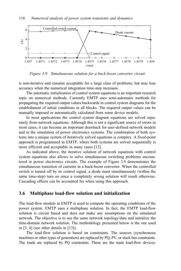
is non-iterative and remains acceptable for a large class of problems, but may loseaccuracy when the numerical integration time-step increases.

The automatic initialization of control system equations is an important researchtopic on numerical methods. Currently EMTP uses semi-automatic methods forpropagating the required output values backwards in control system diagrams for theestablishment of initial conditions in all blocks. The required output values can bemanually imposed or automatically calculated from some device models.

In most applications the control system diagram equations are solved sepa-rately from network equations. Although this is not a significant source of errors inmost cases, it can become an important drawback for user-defined network modelsand in the simulation of power electronics systems. The combination of both sys-tems into a unique system of iteratively solved equations is complex. A fixed-pointapproach is programmed in EMTP, where both systems are solved sequentially ismore efficient and acceptable in many cases [12].

As indicated above, the iterative solution of network equations with controlsystem equations also allows to solve simultaneous switching problems encoun-tered in power electronics circuits. The example of Figure 3.9 demonstrates thesimultaneous transition of currents in a buck-boost converter. When the controlledswitch is turned off by its control signal, a diode must simultaneously (within thesame time-step) turn on since a completely wrong solution will result otherwise.Cascading effects can be accounted for when using this approach.

3.6 Multiphase load-flow solution and initialization

The load-flow module in EMTP is used to compute the operating conditions of thepower system. EMTP uses a multiphase solution. In fact, the EMTP load-flowsolution is circuit based and does not make any assumptions on the simulatednetwork. The objective is to use the same network topology/data and initialize thetime-domain network solution. The methodology presented below is the one usedin [3, 4] (see other details in [13]).

The load-flow solution is based on constraints. The sources (synchronousmachines or other types of generation) are replaced by PQ, PV, or slack bus constraints.The loads are replaced by PQ constraints. These are the main load-flow devices.

1.457 1.4571 1.4572 1.4573 1.4574 1.4575 1.4576 1.4577 1.4578 1.4579 1.4580

2

4

6

t (ms)

(A)

Control signal

Controlled switch currentDiode current

Figure 3.9 Simultaneous solution for a buck-boost converter circuit


All network components must provide a load-flow solution model. For the majority ofdevices, this model is the same as the one used in the steady-state representation.

The system of (3.3) is used for representing the passive network equations, butit must be augmented with load-flow constraint equations. This is another majoradvantage of the augmented formulation approach. The modified-augmented load-flow equations are given by

ALFN AI

LLA Ld

" #Dx

DxLF

" #¼�fLF ð3:41Þ

Equation (3.41) is real, since real and imaginary parts must be represented sepa-rately for load-flow constraints. ALF

N is constructed from the original complexversion of AN by separating real and imaginary parts of each element, AI is aconnectivity matrix for accounting for load-flow devices, and LLA and Ld provideload-flow device constraint equations. The vector function fLF must be minimized(zero) for finding the load-flow solution. It is recalled that the solution offLFðxÞ ¼ 0 can be found using the Newton method:

Jð jÞDxð jÞ¼ �fLFðxð jÞÞ ð3:42Þwhere ð jÞ is the iteration count, J is the Jacobian matrix, and Dx is used in

xð jþ1Þ ¼ xð jÞ þ Dxð jÞ ð3:43ÞEquation (3.41) can be expanded and rewritten as

Yn Ac AIL AIG 0

Ar Ad 0 0 0

JL 0 JLI 0 0

YG 0 0 BGI BGE

JGPQ 0 0 JGPQI 0

JGPV 0 0 0 0

JGSL 0 0 0 0

26666666666664

37777777777775

ð jÞ

DVn

DIx

DIL

DIG

DEG

26666664

37777775¼�

fn

fx

fL

fGI

fGPQ

fGPV

fGSL

26666666666664

37777777777775

ð jÞ

ð3:44Þ

where the submatrices AIL and AIG are adjacency matrices for interfacing the load(IL) and generator (IG) currents with the corresponding passive network nodes. Thefollowing submatrices [13] are used to include load-flow constraints for anynumber of phases: JL and JLI for PQ-loads, YG, BGI, and BGE for generator currentequations, JGPQ and JGPQI for PQ-type generators, JGPV for PV-type generators,and JGSL for slack-type generators (buses). The unknown supplementary vectorsare defined as follows: IL is for PQ-load currents, IG is for generator currents, andEG represents generator internal voltages.

Equation (3.44) is the expanded version of (3.42) and the left-hand side matrixis the Jacobian matrix of the solved nonlinear function fLF.


The linear network coefficient submatrices are copied from the real version(3.4) and remain unchanged, except that now the right-hand side of (3.4) iseliminated due to the differentiation process for the derivation of the Jacobianmatrix. There is no need to derive separate equations for linear network devices.For the ideal transformer case, for example, the constraint equation is takendirectly from (3.14):

Vk2 � Vm2 � gVk1 þ gVm1 ¼ fx ð3:45Þand results into

DVk2 � DVm2 � g DVk1 þ g DVm1 ¼ �f ð jÞx ð3:46Þ

This means that the existing submatrices Ar and Ac are not affected andalready constitute the Jacobian terms allowing to account for all single-phase andthree-phase transformer configurations. The tap positions will affect the ratio g.

3.6.1 Load-flow constraintsEMTP uses constraint equations of load-flow devices which are presented in thissection to demonstrate how such arbitrary equations are entered into (3.44).

In the case of a single-phase load, the PQ constraint can be expressed in termsof load voltage and current. If a load is numbered as p in the list of load devices andconnected between the nodes k and m, its voltage VLp and current ILp are given by

VLp ¼ V Rk þ jV I

k � V Rm � jV I

m ¼ V Rkm þ jV I

km

ILp ¼ IRpkm

þ jI Ipkm

ð3:47Þ

where the superscripts R and I stand for real and imaginary parts, respectively, andthe subscript km means from k to m. The constraint equations become:

Pp � V Rkm IR

pkm� V I

kmI Ipkm

¼ f RLp

¼ 0

Qp � V Ikm IR

pkmþ V R

km I Ipkm

¼ f ILp

¼ 0ð3:48Þ

and the Jacobian terms can now be written as

�IRð jÞpkm

�I Ið jÞpkm

I Ið jÞpkm

�IRð jÞpkm

" #DV R

km

DV Ikm

" #þ �V Rð jÞ

km �V Ið jÞkm

�V Ið jÞkm V Rð jÞ

km

24

35 DIR

pkm

DI Ipkm

" #¼

�f Rð jÞLp

�f Ið jÞLp

24

35 ð3:49Þ

The voltage and current coefficient matrices populate the matrices JL and JLI

(of (3.44)), respectively. The right-hand side is entered into the vector fL of (3.44).In EMTP the three-phase load devices are created from three single-phase loads.The load can be connected in arbitrary configurations.

In EMTP the current constraint of a three-phase generator numbered as p in thelist of generators and connected between buses k and m takes the following form:

YGpðVk � Vm � ~EGpÞ � IGp ¼ fGIp ¼ 0 ð3:50Þ


This is a three-phase and complex system of equations. The generator currents inthe vector IGp are entering bus k, the matrix YGp is the internal admittance matrix,and the vector ~EGp

holds the internal positive sequence voltages and can be writtenas EGp ¼ 1 a2 a

TEGp with a ¼ 1ff120� and the scalar EGp being the voltage

of phase A. Equation (3.50) is rewritten as

YGpDVk � YGpDVm � BGEpDEGp � DIGp ¼ �f ð jÞGIp

ð3:51ÞIn this case YGp populates YG, BGEp is entered into BGE, and the identity

coefficient matrix of DIGp contributes to BGI. In addition, DEGp 2 DEG, DIGp 2 DIG

and fGIp 2 fGI.In addition to (3.50), each generator must provide its equations for controlled

quantities. In the case of PQ control, the Jacobian terms are similar to (3.49), exceptthat now the left-hand side voltage and current vectors are three-phase whichresults into two 6 by 6 coefficient matrices contributing into JGPQ and JGPQI. Theright-hand side is now related to fGPQ.

For the case of PV control, the Q row of PQ control is replaced by the voltageconstraint equation. The control is on the voltage magnitude Vp ( pth generator) ofone phase and gives:

Vp �ffiffiffiffiffiffiffiffiffiffiffiffiffiffiffiffiffiffiffiffiffiffiffiffiffiffiffiffiffiffiffiffiffi

V Rp

� �2 þ V Ip

� �2r

¼ fGPVp ¼ 0 ð3:52Þ

The contribution to (3.44) is found from:

� V Rp

� �2þ V I

p

� �2� ��1

2

V Rð jÞp DV R

p þ V Ið jÞp V I

p

� �¼ �f ðkÞGPVp

ð3:53Þ

and affects JGPV and fGPV. It is not complicated to extend (3.52) to control thepositive sequence voltage magnitude by calculating it from the Fortescue trans-formation for positive sequence.

For the slack bus case it is necessary to write two equations (real and imaginaryparts) for controlling the positive sequence voltage magnitude and phase.

3.6.2 Initialization of load-flow equationsTo initialize its load-flow equations, EMTP uses a linearized version of (3.44). Allloads are replaced by equivalent impedances calculated at nominal voltages and allgenerators are replaced by ideal sources behind their impedances. This approachyields sufficiently good initial conditions for the fast convergence of (3.44).

3.6.3 Initialization from a steady-state solutionUpon convergence of (3.44), all steady-state phasors become available in EMTP.The synchronous machine phasors are used to calculate internal state variables. Theasynchronous machine requires the calculation of slip for a given mechanicalpower or torque.


The steady-state module starts with the load-flow solution and replaces alldevices by lumped equivalents to proceed with a phasor solution. This is achievedwith (3.15). The resulting solution is the same as with the load-flow module, exceptthat now all device models have access to internal phasors for proceeding withinitialization. The steady-state solution phasors are used for initializing all state-variables at the time-point t ¼ 0. The solution at t ¼ 0 is only from the steady-stateand all history terms for all devices are initialized for the first solution time-point.

3.7 Implementation

The matrix AN of an arbitrary network is normally sparse. A block diagonalstructure results when the network contains transmission lines or cables. EMTPuses a sparse matrix solver for its load-flow (see (3.44)), steady-state (see (3.15)),and time-domain (see (3.19)) equations.

The direct approach is used with LU factorization. For the given sparse matrix A:

Ax ¼ LðUxÞ ¼ b ð3:54Þwhere L and U are lower and upper triangular matrices, respectively. Special orderingtechniques can be used to generate row and column permutations and reduce fill-induring factorization. Minimum degree ordering is currently used in EMTP.

Recently the KLU solver has been established as one of the most effectivesolvers for circuit simulation problems [14–16]. The KLU solver permutes thematrix A to obtain the Block Triangular Form (BTF) before ordering. The BTF ofA results into the new matrix A0:

PAQ ¼

A011 A0

12 . . . A014

0 A022

..

.

0 0 . .. ..

.

0 0 0 A0nn

2666664

3777775 ð3:55Þ

where P and Q are column and row permutation matrices, respectively. The BTFprovides important advantages. The diagonal blocks can become independent andhence only these blocks require factorization. The off-diagonal non-zeroes do notcontribute to any fill-in. When a network contains delay-based line/cable models,the BTF allows us to automatically formulate the block-diagonal version of A. Theindependent blocks can be solved in parallel. This method is currently available inEMTP for testing and generalization.

3.8 EMTP models

The basic modeling theory used in EMTP originates from [17], but severalimprovements have been made through ongoing research and within the new pro-gramming environment and computational engine of EMTP. A collection of built-in


models, referred to as primitive models, is used to construct assembled models. Theprimitive control block diagram models are used, for example, to construct governorand exciter models, metering devices, arc models, and various other models.

The models are programmed using an object-oriented approach. Each modelis given its set of data fields and methods. The interaction with the core code ispresented in Figure 3.10. The models receive requests (method calls) and mayparticipate by sending back the required data. This approach decouples completelythe models from the code and provides both flexibility and encapsulation. Themodel development is completely independent from the core code. The models canbe implemented directly or through standard libraries and DLLs (see below).

The rotating machine models are based on Park’s transformation (dq0). Themachine models [18, 19] are interfaced using Norton equivalents. In addition tointernal iteration loops [18, 19], it is optionally possible to iterate the machineequations with the main network equations to achieve highest accuracy levels [20].The importance of such an interface in practical applications is demonstrated in[20]. The machine models participate into all solution modules and it is possible toinitialize them under unbalanced network conditions.

In addition to constant parameter transmission line and cable models, EMTPuses frequency-dependent models based on [21–24].

The EMTP model libraries include numerous components, such as powerelectronics switching devices and converters; HVDC converters; breakers; idealswitches; transformers; arresters; rotating machines; wind generators; line/cabledate calculation tools; lines and cables; measuring devices; control system com-ponents; and various source functions.

EMTP does not require any compiler to perform simulations with its built-inmodels.

3.9 External programming interface

EMTP allows the development of user-defined models and interacts with itscomputational core, using various interfacing techniques. The dynamic link library(DLL) setup offers an elaborate programming interface that allows the building

Data

Core code

Organizer

Solver

Device modelsdata, methods

Scopes, external interaction

Request

Participation

Figure 3.10 EMTP architecture for interfacing its core code with device models


of user-defined models and interacts with the computational engine optionsand matrices. DLL-based models can access and respond to the same requests(methods) as the built-in models. DLL-based models are assembled and compiledindependently from the main EMTP code and can be based on any programminglanguage. The DLL approach is also used in EMTP for interfacing with modelsbuilt in external applications, such as Simulink� [25].

The DLLs can be programmed and built using compilers for the user selectedprogramming language.

3.10 Application examples

EMTP can be used to simulate generic and very large-scale power systems. It doesnot have memory constraints and can automatically allocate memory according tosimulated network requirements. EMTP applications include:

● switchgear, TRV, shunt compensation, current chopping, delayed-current zeroconditions

● insulation coordination● saturation and surge arrester influences● harmonic propagation, power quality● interaction between compensation and control● wind generation, distributed generation● precise determination of short-circuit currents● detailed behavior of synchronous machines and related controls, auto-excitation,

subsynchronous resonance, power oscillations● protection systems● distribution system analysis: unbalanced load-flow, protection, renewable

energies● HVDC systems, power electronics, FACTS and Custom Power controllers

These applications are in a wideband range of frequencies.

The following illustrative examples are presented below to provide a short listof EMTP simulation capabilities. The objective of EMTP is to allow users tosimulate various power system events for a wideband frequency range, using thesame data set and with no user intervention for supporting the solution methods. Itis not necessary, for example, to insert artificial delays between network portionsand control system equations or to insert artificial devices for helping convergenceor solving accuracy/robustness issues.

The graphical user interface of EMTP also allows us to work with variouslevels of complexity by scripting study scenarios and data.

3.10.1 Switching transient studiesA typical switching transient simulation case is presented in Figure 3.11. Thistransient is due to the energization of a transformer in the 500 kV network con-nected to BUS2 in Figure 3.2. A harmonic resonance is observed and the transient


results into a temporary overvoltage condition. It is apparent from the zoomedvoltage of phase-a in Figure 3.11(d) that the network is in steady-state (auto-matically initialized from its load-flow solution) before transformer energizationat 20 ms.

(a) Phase-a voltage, bus BUS2

(b) Phase-b voltage, bus BUS2

(c) Phase-c voltage, bus BUS2

(d) Phase-a voltage, bus BUS2, zoomed version

0 0.5 1 1.5 2 2.5 3 3.5 4

–1

0

1

2

Time (s)

(pu)

0 0.5 1 1.5 2 2.5 3 3.5 4–2

–1

0

1

2

Time (s)

(pu)

0 0.5 1 1.5 2 2.5 3 3.5 4–2

–1

0

1

2

Time (s)

(pu)

0 0.05 0.1 0.15 0.2 0.25 0.3 0.35 0.4 0.45 0.5

–1

0

1

2

Time (s)

(pu)

Figure 3.11 Transients resulting from transformer energization, test case ofFigure 3.2


Since the test case of Figure 3.2 includes synchronous machine models withvoltage regulator and governor controls, it can be also used to study electro-mechanical transients. A single-phase-to-ground fault occurs at 100 ms on the lineside of the breaker 120 k of the line TLM_120mi. The line is opened at both ends at200 ms, the fault is eliminated and the line breakers are reclosed at 400 ms.Figure 3.12 presents the simulation results for generator powers and demonstratesthat the system is able to regain stability for this event. It is apparent that thesynchronous machines are accurately initialized from the load-flow solution beforethe applied perturbation and the automatic initialization process includes the initi-alization of synchronous machine controls. It is noticed that some transmissionlines in this test case are not transposed and some loads are not balanced, but thesynchronous machine and network equations are correctly initialized through theutilized unbalanced load-flow and steady-state solutions.

3.10.2 IEEE-39 benchmark bus exampleIn this test case, the IEEE-39 bus system shown in Figure 3.13 is assembled usingconstant-parameter transmission lines, synchronous machines with magnetizationdata, governor, and exciter controls for synchronous machines, transformermodels with magnetization branch and load models. In this case, the load modelsare dynamic voltage and frequency-dependent models [26]. This type of systemsetup can be used for both electromagnetic and electromechanical transientsimulations.

The simulation results presented in Figures 3.14 and 3.15 are for a single-phase-to-ground fault occurring near bus B3 on the line side of the breaker (seeFigure 3.13). The permanent fault occurs at 200 ms and the line breakers are trippedat both ends at 300 ms. Once again, the network solution is in complete steady-stateat the startup of the time-domain solution.

0 0.5 1 1.5 2 2.5 3–200

0

200

400

600

800

Time (s)

(MW

)

SM6

SM3SM4

SM8 SM11

Figure 3.12 Electromechanical transients, synchronous machine powers, testcase of Figure 3.2


SM B37

PowerPlant_08

SM

PowerPlant_10

B30

SM PowerPlant_09B38

SM

PowerPlant_06

B35

SM

PowerPlant_01

SM

B31AndLoadSLACK

PowerPlant_02

SM

PowerPlant_03B32

SM PowerPlant_05B34

SM

PowerPlant_04B33

SM

PowerPlant_07

B36

+317.70

bus26_28+

101.20

bus28_29

+418.90

bus26_29

Load29Load26

+216.50

bus25_26

Load28Load25

PI+

bus0

2_25

58km

CP

+bus0

2_03

101.

20

+bu

s03_

18

89.1

0Load18

Load3

PI+

bus0

1_02

276k

m+

bus0

1_39

167.

60

+bus0

3_04

142.

80

Load4

Load39 +bu

s04_

05

85.8

0

PI+

bus0

5_06

17km

+bus0

6_07

61.7

0

Load7

PI+

31km

bus0

7_08

+bu

s05_

08

75.1

0

+bu

s09_

3916

7.60

+bu

s08_

09

243.

30

Load8

+bus2

6_27

98.5

0+bu

s17_

2711

6.00

PI+

bus17_18

55km

PI+

bus1

6_17

60km

PI

+

bus1

6_24

40km

+bu

s15_

16

63.0

0 +bu

s16_

21

90.5

0

+bu

s14_

15

145.

40

+bu

s16_

19

130.

70

+bus2

2_23

64.3

0

+bus2

3_24

234.

60

+bus21_22

93.80

+bus04_14

86.50

PI+

bus0

6_11

55km

2 3

1

xfo19_20530/300/12.5

tap=1.061400MVA

+bu

s13_

14

67.7

0

PI+

29km

bus1

0_13

PI

+

29km

bus1

0_11

Load27

Load24

Load16

Load12

Load20

Load23

Load15

+

BUS24_shunt

368uS92MVAR@500kV

Load21

F

Faul

t

BRKB3B4

BRKB4B31

2 -30

503/25

xfo1

2_13 200MVA

tap=1.006

12 -3

0

503/25xfo1

2_11

200MVAtap=1.006

B291.04/_-0.7

B28

1.04/_-3.4

B251.05/_-5.7

B2 1.04/_-7.1

B11.04/_-9.8

B70.98/_-11.2

B39

1.03/_-11.4

1.02/_-11.6B9

B8

0.98/_-11.7

B27 1.02/_-8.9

B26

1.04/_-6.9

B171.02/_-8.7

B181.01/_-9.6

B231.04/_-0.8

B241.02/_-7.4

B221.04/_-0.6

B21

1.02/_-5.1

B60.99/_-8.9

1.00/_-7.2

B11

B191.04/_-2.4

B13

1.00/_-7.1

B101.00/_-6.4

0.98/_-3.4300kV

B20

1.02/_-7.5B16B3

1.01/_-9.9

B140.99/_-8.8

B50.99/_-9.6

0.98/_-10.81.00/_-9.1

B15

0.97/_-37.3 B12

0.98/_-10.8B4

Figure 3.13 IEEE-39 benchmark version simulated in EMTP

0 1 2 3 4 5 6 7 8 9 10100200300400500600700

Time (s)

(MW

)

Figure 3.14 Power from synchronous generator PowerPlant_08, fault near busB3 in Figure 3.13

3.10.3 Wind generationIn this test case the IEEE-39 benchmark is modified to include wind generation.The wind parks are connected to the busses B1, B2, and B25 (Figures 3.16 and 3.17)for a total generation of 755 MW. The synchronous generators on buses B2 and B25

0 0.1 0.2 0.3 0.4 0.5 0.6–4

–2

0

2

4 × 104

Time (s)

(A)

Figure 3.15 Synchronous generator PowerPlant_10 phase currents, fault nearbus B3 in Figure 3.13

+bus25_26

216.50

Load25

PI+

58km

bus02_25

CP

+101.20

bus02_03PI+

276km

bus01_02

Onshore_WP1

Onshore_WP2

V1:1.02/_-5.3

B1

B2 V1:0.99/_-5.3

B25V1:0.99/_-4.9

Figure 3.16 Integration of wind generation into the IEEE-39 benchmark shown inFigure 3.13


B1

BW

12

TR1

500/

220

PI+

TR1_

to_W

P1

PI+

WP2

_to_

WP3

PI+

WP1

_to_

WP2

PI+

WP3

_to_

TR2

Type

-III

(4

5 �

1.5

MW

)

WP1

Type

-III

(4

5 �

1.5

MW

)

WP2

Type

-IV

(2

� 3

0 �

2 M

W)

WP3

+-1

|1E1

5|0

CB

23+

-1|1

E15|

0

CB

321

2TR2

315/

220

+ -1|1

.1|0

CB

_TR

2_in

+-1

|1.1

|0

CB

_TR

2_ou

t

F

Fault

Fig

ure

3.17

Win

dpa

rkO

nsho

re_W

P1

subn

etw

ork

cont

ents

(see

Fig

ure

3.16

)

are now removed. The design of wind park Onshore_WP1 is presented inFigure 3.17. Both wind parks (Onshore_WP1 and Onshore_WP2) contain aggre-gated wind parks with a combination of wind turbines of Type III and Type IV. Thewind generator subnetwork contents for the Type III version are shown in Fig-ure 3.18. The asynchronous generator is modeled with full details, but an averagevalue model is used in this case for the converters. The detailed (IGBT modelbased) converter model is available as an option, but its increased accuracy isunnecessary for this study. The control system subnetwork is presented in Fig-ure 3.19. It includes the protection systems, grid and rotor side converter controls,and pitch control. The setup of controls is the same for both average value anddetailed converter models.

The simulation results shown in Figures 3.20 and 3.21 are for a three-phase-to-ground fault occurring at 1 s (see location in Figure 3.17) and cleared by thebreakers at 1.1 s. The initialization of wind generators is based on startup fromload-flow solution and initial connection to an ideal source. The ideal source isswitched off at 200 ms.

3.10.4 Geomagnetic disturbancesIn this example, the IEEE-39 bus system in Figure 3.22 is used to study geo-magnetic disturbances (GMDs). The Geoelectric Field (GEF) is modeled with adc voltage source injected in series with each transmission line. All transformers

WIND TURBINE

WIND MODEL

ASYNCHRONOUS generator &AC/DC/AC CONVERTER

CONTROL SYSTEM

GEN_BUS

WIND

beta

WIND_TURBINE

ASM

DFIG_hardwareAVM1

pitc

h

crow

bar_

activ

e

w_r

otor

_rad

sV

dc_V

Vab

c_gr

id_V

Iabc

_grid

_AIa

bc_r

otor

_AIa

bc_s

tato

r_A

Iabc

_con

verte

r_A

switc

h_on

chop

per_

activ

e

Vre

f_ro

tor

Vre

f_gr

idbl

ock_

grid

bloc

k_ro

tor

CONTROL

Figure 3.18 Wind generator subnetwork, Type III wind generator model


switc

h_on

pitc

hch

oppe

r_ac

tive

crow

bar_

activ

e

Page

w_r

otor

Vre

f_ro

tor

Vre

f_gr

id

bloc

k_ro

tor

bloc

k_gr

id

Vab

c_gr

id_V

Iabc

_grid

_A

Iabc

_rot

or_A

Iabc

_sta

tor_

A

Iabc

_con

verte

r_A

Vdc

_V

Prot

ectio

n Sy

stem

chop

per_

activ

e

switc

h_on

Vdc

_mea

s

Vab

c_gr

idcr

owba

r_ac

tive

Iabc

_rot

orIa

bc_c

onve

rter

RSC

_blo

ckG

SC_b

lock

Prot

ectio

n

Low

_pas

s filt

er2n

d or

der

LP_f

ilter

Page

P

Con

vert

to p

u

SI - >

pu

conv

_to_

pu

w_r

otor

_rad

s

Com

putin

g V

aria

bles

thet

a_ro

tor_

rad

w_r

otor

Iabc

_rot

orIa

bc_s

tato

r

Iabc

_con

verte

r

w_r

otor

_mea

s

Idq_

conv

erte

rV

dq_g

rid

Idq_

roto

rId

q_st

atorP

thet

a_gr

id_r

ad

Vab

c_gr

idIa

bc_g

rid

Q

Vgr

id

w_s

tato

r

Vdc

_mea

s

Vdc

Com

putin

g_V

aria

bles

Page

Page

P

Gri

d C

ontr

ol

thet

a_gr

id_r

ad

Vre

f_PW

MV

dq_g

ridId

q_co

nver

ter

Vdc

w_s

tato

rGrid

_Con

trol

Rot

or C

ontr

ol

w_r

otor

Vdc

thet

a_ro

tor_

rad

Idq_

stat

orId

q_ro

tor

Vre

f_PW

M

P QVgr

id

w_s

tato

rRot

or_C

ontro

l

Pitc

h C

ontr

ol

Pw_r

otor

Pitc

h_de

g

Pitc

h_C

ontro

l

w_r

otor

Fig

ure

3.19

Typ

eII

Iw

ind

gene

rato

rco

ntro

lsy

stem

(see

subn

etw

ork

inF

igur

e3.

18),

top

leve

lsu

bnet

wor

ks

are modeled appropriately with magnetization data [27] and on load tap changer(OLTC) functionality for studying voltage regulation and voltage collapse con-ditions. The synchronous generator automatic voltage regulators include over-excitation limiters. Other details on this system setup and simulation results canbe found in [27].

Such detailed modeling allows the accurate simulation of GMDs on powersystems and predict voltage collapse conditions resulting from supplementary varconsumptions by network transformers submitted to dc currents. In this type ofanalysis, the simulation interval must be extended to 600 s and highest accuracy isachieved using a numerical integration time step of 50 ms.

3.10.5 HVDC transmissionAn example of HVDC transmission model simulated in EMTP is shown inFigure 3.23. The HVDC converters are modular multilevel converters (MMCs).The detailed simulation of such converter [28–30] requires modeling very large

0 0.5 1 1.5 2 2.5 30

2

4

6

8 × 107

Time (s)

(W)

Figure 3.20 Active power output from WP3 (second wind generator on the right)in Figure 3.18

0.9 0.95 1 1.05 1.1 1.15

–2,000

–1,000

0

1,000

2,000

Time (s)

(A)

Figure 3.21 Currents measured by breaker CB_TR2_out in Figure 3.17


GMD Field Voltage Definitionx+ == Nord-South, y+ == East-West.

SM

PowerPlant_08

B37

SM

B30

PowerPlant_10

SMB38

PowerPlant_09

SM B35

PowerPlant_06

SMPowerPlant_01

SM

PowerPlant_02B31AndLoadSLACK

SM

B32PowerPlant_03

SM B34PowerPlant_05

SM

B33PowerPlant_04

SM B36

PowerPlant_07

+bus26_28

317.70+bus28_29

101.20

+bus26_29

418.90Load29Load26

+bus25_26

216.50

Load28

Load25PI

+58

km

bus0

2_25

CP

+

101.

20bu

s02_

03

+89

.10

bus0

3_18

Load18

Load03

PI+

276k

m

bus0

1_02

+16

7.60

bus0

1_39

+ 142.

80

bus0

3_04

Load04

Load39

+85

.80

bus0

4_05

+

61.7

0bu

s06_

07

Load07

PI+

bus0

7_08

31km

+75

.10

bus0

5_08

+

167.

60bu

s09_

39

+24

3.30

bus0

8_09

Load08

+ 98.5

0

bus2

6_27

+ 116.

00

bus1

7_27

PI+55km

bus17_18

PI

+

60kmbus16_17

+63

.00

bus1

5_16

+14

5.40

bus1

4_15

+13

0.70

bus1

6_19

+64

.30

bus2

2_23

+ 234.

60

bus2

3_24

+93.80

bus21_22

+86.50

bus04_14

PI+

55km

bus0

6_11

+67

.70

bus1

3_14

PI+

bus1

0_13

29km

PI+

bus1

0_11

29km

Load27

Load24

Load16

Load12

Load20

Load23

Load15

+

92MVAR@500kV 368uSBUS24_shunt

Load21

12

200MVAtap=1.006

xfo1

2_11 503/25

12

200MVAtap=1.006

xfo1

2_13 503/25

23 1

xfo19_20

+

+

+

+

+

+

+

+ +

+

+

++

+

+

+

+ ++

+

+

+

++

++

+

field_x

field_y

2.0V/km, 45deg

f(u)time

x

y

PVdc

Vdc

Vdc

Vdc

VdcVdc

Vdc

Vdc

Vdc

PI

+

40km

bus1

6_24

Vdc

Vdc Vdc

Vdc

Vdc

Vdc

Vdc Vdc

Vdc

Vdc

+90

.50

bus1

6_21

Vdc

Vdc

Vdc

+

Vdc

+

Vdc

Vdc

+

Vdc

PI+

17km

bus0

5_06

+

+

VdcVdc

VdcVdc

VdcVdc

Vdc

+

Vdc

+

Vdc

1.05/_-5.9 B25

1.04/_-10.0B1

B7

B91.02/_-11.7

B8

B18

B23

B22

B6

B111.00/_-7.3

1.00/_-7.2B13

B10501.61/_-6.5

B5

B4 B15 1.00/_-9.2

B120.97/_-37.4

1.04/_-0.8B29

1.04/_-7.2B2

B14

B39

1.02/_-7.7B16

B17

B27

1.02/_-7.6B24

1.04/_-7.1B26 B28

B3

0.98/_-3.2 300kVB20

B19

B21

-30

-30

Figure 3.22 IEEE-39 benchmark version modified for GMD studies in EMTP

PQ1 MMCVSC_1

P2

N2N1

Cable_70kmPQ2

+

The equivalent source includesalso a load-flow device

Equivalent_source2

+

The equivalent source includesalso a load-flow device

Equivalent_source1

MMCVSC_2

P1

Figure 3.23 MMC-HVDC transmission system


numbers of nonlinear switching devices. Other types of models can be used inEMTP to reduce computing times. Detailed simulation results and analysis on suchsystems with EMTP can be found in [28–30].

3.10.6 Very large-scale systemsEMTP can be used to simulate very large-scale systems. Such a case is presented in[31]. Much larger systems can be simulated for distribution networks [32].

3.11 Conclusions

This chapter presented a summary on numerical methods used in EMTP (EMTP-RV version) for the computation of electromagnetic transients. EMTP offersseveral options and modules for the simulation and analysis of complex powersystems. EMTP offers a unified environment that can be applied to study powersystems from steady-state conditions, to electromechanical and electromagnetictransients.

References

[1] www.emtp.com[2] J. Mahseredjian, F. Alvarado, ‘‘Creating an electromagnetic transients pro-

gram in MATLAB�: MatEMTP,’’ IEEE Trans. on Power Delivery, vol. 12,no. 1, pp. 380–388, January 1997.

[3] J. Mahseredjian, S. Dennetiere, L. Dube, B. Khodabakhchian, L. Gerin-Lajoie, ‘‘On a new approach for the simulation of transients in power sys-tems,’’ Electric Power Systems Research, vol. 77, no. 11, pp. 1514–1520,September 2007.

[4] J. Mahseredjian, ‘‘Simulation des transitoires electromagnetiques dans lesreseaux electriques,’’ Edition ‘Les Techniques de l’Ingenieur’, February 10,2008, Dossier D4130. 2008, 12 pages.

[5] B. Kulicke, ‘‘(Simulation program NETOMAC: Difference conductancemethod for continuous and discontinuous systems),’’ Siemens Forschungs—und Entwicklungsberichte—Siemens Research and Development Reports,vol. 10, no. 5, pp. 299–302, 1981.

[6] J. R. Marti, J. Lin, ‘‘Suppression of numerical oscillations in the EMTPpower systems,’’ IEEE Trans. on Power Systems, vol. 4, no. 2, pp. 739–747,1989.

[7] F. H. Branin, ‘‘Computer methods of network analysis,’’ Proc. of IEEE,vol. 55, no. 11, pp. 1787–1801, November 1967.

[8] H. W. Dommel, ‘‘Digital computer solution of electromagnetic transients insingle- and multiphase networks,’’ IEEE Trans. on Power Apparatus andSystems, vol. 88, no. 4, pp. 734–741, April 1969.


[9] L. W. Nagel, ‘‘SPICE2 A computer program to simulate semiconductorcircuits,’’ Memorandum No. UCB/ERL M520, May 9, 1975.

[10] M. Tiberg, D. Bormann, B. Gustavsen, C. Heitz, O. Hoenecke, G. Muset,J. Mahseredjian, P. Werle, ‘‘Generic and automated simulation modelingbased on measurements,’’ Proc. of International Conference on Power Sys-tems Transients, IPST 2007 in Lyon, France, June 3–7, 2007.

[11] J. Mahseredjian, C. Dufour, U. Karaagac, J. Belanger, ‘‘Simulation of powersystem transients using state-space grouping through nodal analysis,’’ Proc.of International Conference on Power Systems Transients, IPST 2011 inDelft, Netherlands, June 14–17, 2011.

[12] J. Mahseredjian, L. Dube, M. Zou, S. Dennetiere, G. Joos, ‘‘Simultaneoussolution of control system equations in EMTP,’’ IEEE Trans. Power Sys-tems, vol. 21, no. 1, pp. 117–124, February 2006.

[13] I. Kocar, J. Mahseredjian, U. Karaagac, G. Soykan, O. Saad, ‘‘Multiphaseload flow solution of large scale distribution systems using the MANAapproach,’’ IEEE Trans. on Power Delivery, vol. 29, no. 2, pp. 908–915,April 2014.

[14] T. A. Davis, E. P. Natarajan, ‘‘Algorithm 907: KLU, a direct sparse solverfor circuit simulations problems,’’ ACM Transactions on MathematicalSoftware, vol. 37, no. 3, pp. 36:1–36:17, September 2010.

[15] S. A. Hutchinson, E. R. Keiter, R. J. Hoekstra, L. J. Waters, T. Russo,E. Rankin, S. D. Wix, C. Bogdan, ‘‘The XyceTM parallel electronicsimulator—an overview,’’ IEEE International Symposium on Circuits andSystems, Sydney (AU), May 2000.

[16] E. P. Natarajan, ‘‘KLU A high performance sparse linear solver for circuitsimulation problems,’’ Master’s Thesis, University of Florida, 2005.

[17] H. W. Dommel, EMTP Theory Book, Portland, Oregon: Bonneville PowerAdministration, 1996.

[18] U. Karaagac, J. Mahseredjian, O. Saad, ‘‘An efficient synchronous machinemodel for electromagnetic transients,’’ IEEE Trans. on Power Delivery,vol. 26, no. 4, pp. 2456–2465, October 2011.

[19] U. Karaagac, J. Mahseredjian, O. Saad, S. Dennetiere, ‘‘Synchronousmachine modeling precision and efficiency in electromagnetic transients,’’IEEE Trans. on Power Delivery, vol. 26, no. 2, pp. 1072–1082, April 2011.

[20] U. Karaagac, J. Mahseredjian, I. Kocar, O. Saad, ‘‘An efficient voltage-behind-reactance formulation based synchronous machine model for elec-tromagnetic transients,’’ IEEE Trans. on Power Delivery, vol. 28, no. 3,pp. 1788–1795, April 2013.

[21] J. R. Marti, ‘‘Accurate modeling of frequency-dependent transmission linesin electromagnetic transient simulations,’’ IEEE Transactions on PowerApparatus and Systems, vol. 101, no. 1, pp. 147–155, January 1982.

[22] A. Morched, B. Gustavsen, M. Tartibi, ‘‘A universal model for accuratecalculation of electromagnetic transients on overhead lines and undergroundcables,’’ IEEE Trans. on Power Delivery, vol. 14, no. 3, pp. 1032–1038, July1999.


[23] I. Kocar, J. Mahseredjian, G. Olivier, ‘‘Improvement of numerically stabilityfor the computation of transients in lines and cables,’’ IEEE Trans. on PowerDelivery, vol. 25, no. 2, pp. 1104–1111, April 2010.

[24] I. Kocar, J. Mahseredjian, G. Olivier, ‘‘Weighting method for transientanalysis of underground cables,’’ IEEE Trans. on Power Delivery, vol. 23,no. 3, pp. 1629–1635, July 2008.

[25] www.mathworks.com[26] IEEE Task Force on Load Representation for Dynamic Performance. Load

Representation for Dynamic Performance Analysis. IEEE Transactions onPower Systems, vol. 8, no. 2, pp. 472–482, May 1993.

[27] L. Gerin-Lajoie, J. Mahseredjian, S. Guillon, O. Saad, ‘‘Simulation ofvoltage collapse caused by GMDs—problems and solutions,’’ CIGREConference, Paris, August 24–28, 2014.

[28] J. Peralta, H. Saad, S. Dennetiere, J. Mahseredjian, S. Nguefeu, ‘‘Detailedand averaged models for a 401-level MMC-HVDC system,’’ IEEE Trans. onPower Delivery, vol. 27, no. 3, pp. 1501–1508, July 2012.

[29] H. Saad, J. Peralta, S. Dennetiere, J. Mahseredjian, et al., ‘‘Dynamic aver-aged and simplified models for MMC-based HVDC transmission systems,’’IEEE Trans. on Power Delivery, vol. 28, no. 3, pp. 1723–1730, July 2013.

[30] H. Saad, S. Dennetiere, J. Mahseredjian, et al., ‘‘Modular multilevel con-verter models for electromagnetic transients,’’ IEEE Trans. on PowerDelivery, vol. 29, no. 3, pp. 1481–1489, June 2014.

[31] L. Gerin-Lajoie, J. Mahseredjian, ‘‘Simulation of an extra large network inEMTP: from electromagnetic to electromechanical transients,’’ Proc. ofInternational Conference on Power Systems Transients, IPST 2009 inKyoto, Tokyo, June 2–6, 2009.

[32] V. Spitsa, R. Salcedo, R. Xuanchang, J. F. Martinez, R. E. Uosef, F. de Leon,D. Czarkowski, Z. Zabar, ‘‘Three-phase time–domain simulation of verylarge distribution networks,’’ IEEE Trans. on Power Delivery, vol. 27, no. 2,pp. 677–687, 2012.


Chapter 4

PSCAD/EMTDC

D. Woodford*, G. Irwin* and U.S. Gudmundsdottir†

4.1 Introduction

During the early 1970s, Manitoba Hydro was building the Nelson River DCTransmission System to bring hydroelectric power from Northern Manitoba toWinnipeg. At that time, Hydro Quebec was also developing its northern hydro-electric resources and had created IREQ (Hydro Quebec Research Institute) toassist them in their endeavour. IREQ acquired an analogue dc simulator fromEnglish Electric and Manitoba Hydro made good use of it to study their NelsonRiver DC Transmission System. The controls for the dc simulator were the same ason Nelson River DC Bipole 1.

The difficulty with the analogue dc simulator as a study tool was the lengthy set-up and checking time. For a study that lasted 2 weeks, the first 9 days were devoted toset-up and checking, and most of the studies was carried out during the last three hoursbefore the taxi came to drive the team to the airport to return back to Winnipeg.

In 1973, Manitoba Hydro received a copy of the Bonneville Power Adminis-tration’s Electromagnetic Transients Program or EMTP [1], as it later became to becalled. Dennis Woodford tried for 6 months to model a simple dc link on EMTP butgave up in despair. There was no control on modelling capability with EMTP inthose days. So, starting from Hermann Dommel’s classic paper on electromagnetictransients [2], Dennis Woodford wrote in FORTRAN4, the first code of EMTDC.1

After the frustrations for trying to model dc transmission on EMTP, he was carefulnot to look at EMTP code. He did not want to build the limitations of EMTP at thattime into EMTDC.

While working with English Electric in the United Kingdom in the late 1960s,Dennis Woodford made use of a digital controls modelling program known asKALDAS.2 Then at Manitoba Hydro, in the early 1970s, IBM’s CSMP3 controls

*Electranix Co., Canada†Dong Energy, Denmark1EMTDC was the ElectroMagnetic Transients for DC and was developed at Manitoba Hydro as asimulation engine.2‘KALDAS, an algorithmically based digital simulation of analogue computation’. Computer Journal,vol. 9, no. 2, pp. 181–187 (1966).3CSMP, Continuous System Modelling Program. IBM Systems Journal, vol. 6, no. 4, p. 242 (1967).

modelling software was used. Concepts from both these programs were designed toapply building blocks that emulated analogue computer functions. It made sensetherefore to incorporate the concept of these programs into the EMTDC electro-magnetic transients solution to interface with the network solution. The controlfunctions were labelled CSMF or ‘Continuous System Modelling Functions’. TheEMTDC network solution and the controls building blocks of CSMF were suc-cessfully merged so that users could write their own controls system models ina FORTRAN subroutine labelled DSDYN or Digital System DYNamics. Nodevoltages and branch currents could be accessed by the CSMF functions in DSDYNand could control sources, switches and branch inductors, capacitors or resistors.

The very first code of EMTDC contained phasor network solutions as well asthe controls. Eventually, the phasor solution was replaced by the electromagnetictransients solution.

The best way to model a large dc system was still not obvious. In the late1970s, Dennis Woodford had a project meeting in Bismarck, North Dakota for aproposed 500 kV transmission line between Canada and the United States. Theflight to Bismarck was at dawn, but it was fogged in. After several attempts, theplane landed. However, no more planes landed and Dennis was the only one whoarrived for the meeting. The flight out was not until that evening. It was during theday in a quiet corner of Bismarck airport that the concept for modelling large dcsystems in EMTDC was worked out.

At this time, a graduate student at the University of Manitoba, Ani Gole wasinvestigating a project for Manitoba Hydro. He needed a good synchronousmachine model for his study, and with Dr. Rob Menzies at the University ofManitoba, they teamed up with Dennis and produced one. Ani Gole’s project led tohis Ph.D. and he was the first graduate student to use the EMTDC.

Up until 1980 when Ani Gole and Rob Menzies joined the development ofEMTDC, only Dennis Woodford had used the program. He did not publicize hisefforts since every time he raised it for discussion, no support was offered. Engi-neers were quite negative about the possibility that dc transmission could beaccurately simulated digitally. One engineer said he would only believe it is pos-sible if it could model core saturation instability in dc transmission. It was felt thatdigital simulation of dc transmission was impossible to achieve. Without support,there was no chance of corporate funding for a project of ‘dubious’ outcome.Consequently, the development was bootlegged, which as it happens is a veryefficient development method.

The challenge to simulate core saturation instability was considered seriously.This performance problem on the Nelson River HVDC Transmission had occurredon several occasions and could not be reproduced on the analogue dc simulator atIREQ. The simulator’s high level of damping and losses were thought to inhibit theobservation of core saturation instability. Dennis Woodford embarked on a projectto model Bipoles One and Two of the Nelson River HVDC Transmission onEMTDC. Dr. Mohamed Rashwan, the dc engineer at Dorsey Station, was kindenough to provide data on the dc controls and protections that were subsequentlyprogrammed into the EMTDC model. Using recordings from known disturbances,


the EMTDC simulation was tested and found to have good performance by com-parison. John McNichol of Transmission Planning at Manitoba Hydro had systemdata and recordings of a core saturation instability event on the Nelson RiverHVDC Transmission that he was kind enough to share. When the system data wasentered into the simulation model on EMTDC, and the fault that instigated the coresaturation instability was applied, the EMTDC simulation immediately exhibitedthe elusive core saturation instability.

Even despite the success of simulating core saturation instability, there wasstill considerable reticence in accepting EMTDC as the replacement for analoguesimulation. Even Dennis Woodford did not feel completely confident that EMTDCwas simulating the right phenomenon. Another significant study was undertakenthat involved a spurious 93 Hz sustained oscillation on Nelson River Bipole II thatstarted up when its first 500 kV valve group was de-blocked. The EMTDC simu-lation could not reproduce the event. After some time, engineers from the WorkingGroup (BBC, Siemens and AEG), who were the equipment suppliers of Bipole II,were in Winnipeg and a meeting was convened at Dorsey Station to review theproblem. The key components of the EMTDC simulation model was reviewed withthem and everything checked out satisfactorily. The response time of the dc currenttransducers was asked. The reply from the equipment suppliers was ‘instanta-neous’. It was countered that it can’t be instantaneous. The Working Group engi-neers had some discussion among themselves, and it was obvious they didn’t knowand all they agreed on was that it was ‘fast’.

During the modelling of Bipole II on EMTDC, this same question was asked ofMohamed Rashwan who had proposed the dc current transducer response timeconstant be modelled as 10 ms. So, it was reset to 1 ms in the model and thesimulation repeated. Immediately the 93 Hz oscillation appeared. This increasedconfidence in the simulating capability of EMTDC for very complex power systemmodels. It is safe to say that during the early 1980s, this was the largest dc simu-lation model ever produced.

Just because the simulation of the 93 Hz simulation was successful, it did notmean that the reason for it was obvious. It took some time before with the use ofEMTDC, and it was determined to be a ground mode resonant frequency at 93 Hzon the dc transmission line reacting with a positive sequence 153 Hz ac systemresonance generated between the rectifier ac filters and the Long Spruce generatingstation. Since the EMTDC simulation with a slower responding dc current trans-ducer could not generate the offending 93 Hz oscillation, the immediate solutionwas to add a capacitor to the input to the analogue current control amplifier in theBipole II dc controls to effectively slow down the current feedback signal to about a10 ms response time. This solution stayed in effect for many years and the 93 Hzoscillation was never observed again.

In November 1981, the Manitoba HVDC Research Centre was incorporated asan independent non-profit company and EMTDC was given to them by ManitobaHydro for further development and marketing, although Manitoba Hydro retainedits intellectual property rights. The great contribution made by the Manitoba HVDCResearch Centre was the development of the graphical user interface to EMTDC

PSCAD/EMTDC 137

known today as PSCAD.4 Garth Irwin took over development of EMTDC addingsignificant improvements to it and guided the development of PSCAD. Manytalented and capable computer scientists and engineers continue to developEMTDC and PSCAD to this day at the Manitoba HVDC Research Centre, now afully owned subsidiary of Manitoba Hydro.

4.2 Capabilities of EMTDC

The development of EMTDC and PSCAD is guided by the needs of many usersaround the world. The following are some of the studies that can be conducted withPSCAD/EMTDC:

● Insulation coordination of ac and dc equipment, including steep front studies,lightning studies and circuit-breaker transient recovery voltages

● Ease of user-constructed models● Studies of very large systems through hybrid simulation of PSCAD with

PSS�E5 using E-TRAN6

● Designing power electronic systems and controls● Incorporating the capabilities of MATLAB�/Simulink�7 directly into PSCAD● Sub-synchronous oscillations, their damping and torsional interactions● Effects of dc currents and geomagnetically induced currents on power systems,

inrush effects and ferroresonance● Distribution system design with custom power controllers and distributed

generation● Power quality analysis and improvement● Design of modern transportation systems using power electronics (ships, rail,

auto)● Design, control coordination and system integration of wind and solar farms,

diesel systems, energy storage● Sub-synchronous control interactions (SSCI)● Impedance scans of a power system network over a range of frequencies and

contingencies● Under government security, PSCAD has been used to study the impact of

electromagnetic pulse on electric power systems

4PSCAD, Power System Computer Aided Design, the graphical user interface to EMTDC and theproperty of Manitoba Hydro and is developed by the Manitoba HVDC Research Centre (https://hvdc.ca/pscad/).5PSS�E is an integrated, interactive program of Siemens PTI for simulating, analysing and optimizingpower system performance.6E-TRAN by Electranix Corporation for translating steady-state and dynamic data for PSS�E intoPSCAD, for hybrid simulation between PSCAD and PSS�E, and for multi-core processing of PSCAD.7MATLAB/Simulink by MathWorks incorporates MATLAB, the language of technical computing andSimulink, for simulation and model-based design.


The development of frequency-dependent transmission lines and cables pro-vides an important capability for PSCAD. Experts were enlisted to support thisdevelopment and included Bjorn Gustaveson [3], L. Martin Wedepohl [4], GarthIrwin, John Nordstrom, Dr. Ani Gole and his graduate students. Improving theaccuracy of frequency-dependent transmission lines and cables is an ongoingdevelopment for PSCAD.

The User’s Guide on the use of PSCAD is available from the Manitoba HVDCResearch Centre [5].

4.3 Interpolation between time steps

Simplified phasor modelling such as with power system stability programs is farfrom adequate when solid-state switches, circuit breakers, faults, complex controland protection systems require precise representation. This is achieved by electro-magnetic transients programs with varying levels of accuracy depending on thesolution method it applies. Solution methods include (1) forward only time-stepprogressions, whether fixed or variable in time steps where a switching or changeof state can only occur at time points that are a multiple of the time step Dt or(2) interpolation between time steps.

PSCAD applies the principle of interpolation to deal with ensuring a switchingor change of state event occurs at the exact instant in time. This is achieved byallowing the solution to ‘back up’ to the precise instant in time when the change ofstate occurs. The advantages of interpolation are as follows:

● Allows simulation to be run with a larger time step without affecting accuracy.The alternative of changing to smaller time steps when a switching instant isdetected requires a retriangularization of the matrix and in general results inlonger calculation times

● Results in correct theoretical harmonics generated by switching devices(including HVDC and FACTS controllers) because each switch device fires atthe correct time

● Avoids voltage ‘spikes’ in VSC circuits due to incorrect back-diode turn-ontimes (unrealistic snubber circuits are required to control these spikes in fixedtime-step programs)

● Avoids numerical instabilities that can occur due to arrangements of multipleswitching devices in close proximity

● Results in more accurate models of non-linear devices (surge arresters), espe-cially in energy calculations

● Models correctly represent the low-frequency damping and harmonics ofswitching devices interacting with sub-synchronous resonance effects inmachines

The interpolation process applied in PSCAD ensures that any backing up intime is performed using solutions that are calculated by the same conductancematrix. As an example, an IGBT circuit switches when either the voltage or current

PSCAD/EMTDC 139

through it is zero, thus giving the correct losses the IGBT model and network it isembedded in will provide. Other features in the interpolation are as follows:

● Large portions of a network separated by travelling wave transmission lines orcables are separated into sub-systems (so interpolations and switchings areisolated to only the required sub-network without having to manipulate theentire network).

● Control of chatter at inductive nodes and in capacitor loop currents is stillcontrolled using the proven interpolated ½ step chatter removal process.

● The solution can be interpolated numerous times to accommodate multipleswitches that occur in the same time step.

The process of interpolation is demonstrated by current through a simplediode. The waveform in Figure 4.1(a) shows the current through the diode with astandard fixed time-step switching algorithm. The current reverses at some time inbetween time steps Dt and 2Dt, but because of the discrete nature of the time step,the impedance of the device can only be made infinite (i.e. the diode turns off) atintegrals of Dt. Here the simulated diode actually turns of at time 2Dt, whereas inreality the process should have occurred Dt time units earlier. The first recordedinstant of zero current is thus at 3Dt.

Figure 4.1(b) shows the same device with the switching interpolated to thecorrect instant. As before, the program calculates the solution at t ¼ Dt and t ¼ 2Dt.

Id

(a)

(b)

2.0

dt

1.00Id

0Id

3.0

2.02.2

1.01.2

3.03.2

Time (× Δt)

Time (× Δt)

Figure 4.1 Simulated diode switching off at a current zero (a) with fixed time stepand (b) with interpolation


However, on noticing that at the latter time, the current has already crossed zero, itestimates the turn-off time to be t ¼ 1.2Dt based on a linear interpolation of thecurrent within the switching interval. All the voltages and currents in the trape-zoidal solution method are then also interpolated to this intermediate time in alinear fashion. The admittance matrix is then reformulated and the solution con-tinues with the original time step, yielding the new solution one time step later att ¼ 2.2Dt. One additional interpolation step between t ¼ 1.2Dt and 2.2Dt yields thesolution at t ¼ 2Dt. The latter apparently cosmetic step is taken to put the solutionback on the original time grid.

A simple circuit to illustrate the excellent performance of interpolation isshown in Figure 4.2. Here the IGBT is first turned on and current IL ramps upthrough the inductor. Then the IGBT is turned off, and at the same instance, thediode must turn on as the inductor current commutates to it. The commutationprocess is as shown in Figure 4.3.

The success of interpolation is evident in Figure 4.3 as no spikes in voltage andcurrent occur. The simple test circuit of Figure 4.2 without snubbers on the IGBT ordiode is an excellent test for any simulation algorithm.

Although a very simple example has been presented, the interpreted solution isbeing successfully applied to large power electronic simulations without knownlimitations and good speed of simulations [6].

4.4 User-built modelling

PSCAD/EMTDC is a platform for users to build their own models. It is usual formodels to be incorporated into ‘Components’ that may consist of network and/orcontrols and perhaps with user-written descriptive code in FORTRAN or C. Theactual process of creating a Component is not covered in this section. However, if auser-built Component is available and required for simulation, this is the process tobe followed to include in the development of a simulation model for the develop-ment of a Component.

0.1Pulse

IGBT

IL

Idiode

2

D

10 volt dcsource

+–

VL

Figure 4.2 Network for simple test circuit with no snubber damping circuits

PSCAD/EMTDC 141

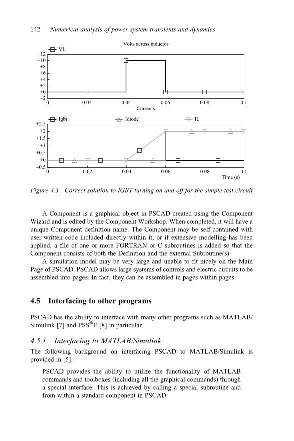
A Component is a graphical object in PSCAD created using the ComponentWizard and is edited by the Component Workshop. When completed, it will have aunique Component definition name. The Component may be self-contained withuser-written code included directly within it, or if extensive modelling has beenapplied, a file of one or more FORTRAN or C subroutines is added so that theComponent consists of both the Definition and the external Subroutine(s).

A simulation model may be very large and unable to fit nicely on the MainPage of PSCAD. PSCAD allows large systems of controls and electric circuits to beassembled into pages. In fact, they can be assembled in pages within pages.

4.5 Interfacing to other programs

PSCAD has the ability to interface with many other programs such as MATLAB/Simulink [7] and PSS�E [8] in particular.

4.5.1 Interfacing to MATLAB/SimulinkThe following background on interfacing PSCAD to MATLAB/Simulink isprovided in [5]:

PSCAD provides the ability to utilize the functionality of MATLABcommands and toolboxes (including all the graphical commands) througha special interface. This is achieved by calling a special subroutine andfrom within a standard component in PSCAD.

0–0.5

+0+0.5

+1+1.5

+2+2.5

0.02 0.04 0.06 0.08 0.1

0–2+0+2+4+6+8

+10+12

0.02 0.04Currents

Volts across inductor

0.06 0.08 0.1

Time (s)

Igbt

VL

Idiode IL

Figure 4.3 Correct solution to IGBT turning on and off for the simple test circuit


Components that interface to MATLAB/Simulink are not offered as part of thePSCAD Master Library and must be specially developed for this purpose. Once thespecial component is developed, it is treated as a normal component in PSCAD. Ofcourse MATLAB/Simulink must be installed on the computer with PSCAD inorder to use the interface component. Instructions in writing a MATLAB or aMATLAB/Simulink interface component are presented in [5] where contact can bemade for help if needed in preparing the interface component.

The MATLAB graphics functions are a very powerful addition to the PSCADplots and graphical interface. Three-dimensional plots, active graphics and rotatingimages are possible and integrate seamlessly with the PSCAD graphical libraries.

An important factor to consider before attempting to interface with MATLABfrom PSCAD: It will not function when using the free GNU FORTRAN77 compiler.

4.5.2 Interfacing with the E-TRAN translatorUsers of electromagnetic transients simulation programs such as PSCAD often facedifficulties in obtaining data and developing cases suitable for their studies. Manyutilities have the data available for their entire system in power flow programs, buta great deal of effort is required to re-enter the network data for use in EMTprograms.

There are three basic challenges:

● Translation of circuit/network data (differences in per-unit systems, dataentry etc.)

● The generation of network equivalents● Initialization of machines, generators or sources in large interconnected networks

E-TRAN will directly create the necessary files for PSCAD from solved PSS/Epower flow and transient stability files. The PSCAD files so translated are completewith correct data for all busses, loads, dc links, switched shunt devices, branches,generators, transformers, phase shifters etc., all correctly drawn and graphicallyinterconnected. E-TRAN translates an entire circuit, a zone or area, or a central busand ‘N busses away’. Network drawings are grouped by location and voltage level,and can be created for a complete network or a portion of a network. The E-TRANfeatures are shown in Figure 4.4.

Further explanation follows.

4.5.2.1 Formation of network equivalentsThe bus voltages and angles and power and reactive power flow information (fromthe solved power flow input file) are used to directly initialize sources/generators inPSCAD (and to initialize non-linear loads etc.). The initialization information canbe used in simple voltage source representations of generators, or can be used toinitialize detailed machines, governors, exciters, multi-mass systems etc. Theresulting simulation in PSCAD exactly matches the solved load flow results forany circuit, and complex systems with any number of machines can be initializedwithout start-up oscillations.

PSCAD/EMTDC 143

The algorithm used to automatically generate the circuit layout in PSCAD isbased purely on busses and connection information (for the PSS/E power flow fileis based on the graph theory).

4.5.2.2 Initialization of machines, generators and sourcesE-TRAN includes a downloadable Runtime Library with the .psl extension for usein PSCAD. The E-TRAN library contains all models used in power flow programsincluding load models, sources, transmission lines, transformers, phase shifters etc.It has data entry based on the same per-unit system and data entry standards as usedin power flow programs. PSCAD cases generated with E-TRAN can be freelydistributed to other users without license fees.

E-TRAN also supports a Substitution Library (also with a .psl extension),which allows a user to maintain and automatically substitute its own more detailedmodels instead of simple power flow data. E-TRAN also reads the standarddynamic models in PSS�E.

E-TRAN generates warnings and error messages when it reads in PSS�E .rawinput files. This will inform the user of areas of mismatched voltage levels,inconsistencies in the entry of data. The result messages are output to the E-TRANlog file.

Substitutionlibrary

Auto-routingand graphicalrepresentation

Initializingmachines,generators

and sources

Translate machinesfrom .dyr file

Sanitycheck and

dataverification

E-TRANruntime

library forPSCAD

Formationof networkequivalents

Translate PSS/E datato PSCAD models

E-TRAN

Figure 4.4 Illustration of the operations of E-TRAN


The user identifies a portion of the network for a direct translation into PSCADmodels (i.e. the ‘kept’ network), and E-TRAN creates a network equivalent of therest of the network based on the available fundamental frequency impedance andpower flow information. The equivalent is a multi-port representation that will becorrect for steady state as well as for open-circuit and short-circuit conditions andcontains Thevenin voltage sources to match PQ flow and represent generationin the equivalent network. The equivalents are generated based on the positivesequence data entered in PSS�E power flow files, and includes the effect ofnegative and zero sequence data if sequence files are available.

E-TRAN generates warnings and error messages when it reads in PSS�Epower flow input files. This will inform the user of areas of mismatched voltagelevels, inconsistencies in the entry of data. The result messages are output to theE-TRAN log file.

The E-TRAN library for PSCAD contains models which mirror the function-ality of the device models contained in PSS/E such as constant power and constantreactive power loads. The E-TRAN program translates the results into PSCAD, andthen the PSCAD differential equation solver is used during the run. The resultingsolution will match the PSS�E power flow results to about three or four decimalpoints everywhere in the system.

E-TRAN generates a complex admittance matrix for the entire system whichcan be greater than 50,000 busses. It then calculates the power and reactive powermismatch of the entire system to see if the input power flow file is solved anddecomposes using LDU sparse decomposition techniques to generate networkequivalents.

4.5.2.3 E-TRAN substitution libraryIf a user has more detailed data available (e.g. geometrical data for transmissionlines suitable for a frequency-dependent line model or a detailed core representa-tion of a transformer with saturation data entered etc.) then the user can maintainthis data in a Substitution Library and E-TRAN can directly write out this datainstead of the simple data used by PSS�E. A device in the Substitution Library canalso be a user-constructed component, in which case it can contain many sub-pagesof electrical or control devices such as a detailed model of an HVDC link or SVC.An initialization feature can be used to define �30 degree phase shifts (due to wye-delta transformers) and to accept the power flow steady-state voltage magnitudeand phase angles. This can be used to initialize any device. The process that indi-cates how the substitution library is a part of the E-TRAN translation procedure isshown in Figure 4.5.

4.6 Operations in PSCAD

4.6.1 Basic operation in PSCADComponents are either network components such as resistors, inductors, capacitors,switches, ac machines, transformers or power electronic devices, or measurement,

PSCAD/EMTDC 145

control, monitoring functions, signal processing, outputs etc. Basic components areavailable in a Master Library.

A valuable feature of PSCAD is the display of output results as the simulationis running. Increased interaction is possible where the user can observe outputresults either as the case is running or with the simulation in ‘pause’.

With the help of ‘fly-by’ monitoring see exactly how the network and controlsare performing, and adjust or switch parameters online as desired. The fly-by helpis operational when the case is running or in ‘pause’ mode.

Initialization of power systems with complex and non-linear power electronicequipment and their controls and protections is undertaken by a run-up to steadystate. A snapshot may be taken when steady state is reached, which becomes theinput data for a study requiring a fully initialized solution. Where E-TRAN is used,it can extract initial conditions from a solved power flow case of the system andinput the initialized states of generators, motors, as well as models extracted fromthe substitution library of E-TRAN. These fully initialized models from E-TRANstay fixed during start-up of a case until the steady state of all the complex non-linear power electronic equipment has been reached and a snapshot taken.

PSCAD provides online plotting of user-selected quantities as well as post-runplotting. Additional plotting programs are available for post-run plotting such asMicrosoft’s Excel program, Livewire8 and TOP.9

4.6.2 Hybrid simulationThe approach taken to implement the hybrid simulation with PSCAD is shown inFigure 4.6, and has been implemented at this time with the PSS�E transient sta-bility program. Hybrid simulation allows the simultaneous use of both PSS�E and

Read E-TRAN Write

PSS/E data files.raw.dyr.seq

PSCAD file.psc

PSCAD filesubstitutionlibrary.psl

Fetch element

Is elementin .psl file?

Check next element

Yes

No

Replace

Figure 4.5 State diagram showing at which stage of a translation E-TRAN checksfor detailed components of the substitution library

8Livewire 2 by Z Systems Inc. See also Manitoba HVDC Research Centre.9TOP, The Output Processor, by Electrotek Concepts, Inc.


PSCAD simulations, taking advantage of the strengths of each program for studycapability that is not possible in either program. The applications for hybridsimulation become exciting, as many of the limitations of each type of simulationprogram will disappear. The PSS�E portion of the simulation models the full acsystem, which includes all electromechanical modes of oscillation. Highly detailedPSCAD models for complex equipment are interfaced to the transient stabilitymodels currently used, and the resulting simulation will be more accurate and runfaster than either program by itself. The combined PSS�E transient stability andPSCAD simulation is capable of modelling more detail using different simulationtime steps, and run each portion of the network separately. There is also the cap-ability of interconnecting two asynchronous electric power systems each modelledin PSS�E through a PSCAD network that includes an HVDC interconnectorbetween the two asynchronous ac systems.

It is possible that each of the separate ac systems can be modelled with dif-ferent versions of PSS�E, and each PSCAD system model can also be with adifferent PSCAD version.

As the hybrid simulation runs, the sub-systems communicate boundary elec-trical conditions with each other at the larger simulation time step. Voltage mag-nitude and angle/frequency information from the transient stability simulation issent to the PSCAD simulation, where it is used to update equivalent voltage sourceson the diagonals of a system equivalent that is auto-created based on the power

G G GPSCAD

CPU #1CPU #1

TCP/IPCommunications

CPU #3

Hybrid PSCAD/Transient Stability Model

Pure TransientStability Model

CPU #2

PSCADG

LargeSystem

Transient Stability Model

LargeSystem

Transient Stability Model

Figure 4.6 Hybrid simulation on multiple CPUs

PSCAD/EMTDC 147

flow admittance matrix. A discrete Fourier transform is used to extract positivesequence power and reactive power from the PSCAD simulation, and transmit it tothe transient stability simulation, where it is used to update a dynamic power andreactive power generator/load model. This in turn acts as a current injection in thetransients simulation to calculate the new voltage at the interfacing point by per-forming a power flow calculation. The two programs run synchronously in time,allowing faults to be made on either side to correctly affect the other.

4.6.3 Exact modelling of power system equipmentEquipment suppliers of wind turbine generators, inverters for solar wind farms,STATCOMs and SVCs, and HVDC converters can supply an exact PSCAD com-ponent model of their equipment including the digital controls, protections and on-off firing pulses to the solid-state valves. The digital code used for controls andprotections can be downloaded into PSCAD and, along with the physical andelectrical stimulation of the equipment, can be provided by the supplier for use inPSCAD, usually in the form of a ‘black box’ and accompanied by a non-disclosureagreement. This has the advantage of having a PSCAD simulation model thatperforms exactly as the real equipment. It has the disadvantage that there is limitedor no adjustment of control or protection settings by the user and such models canonly be used for applications with the consent of the equipment supplier.

The PSCAD black box component models provided by equipment suppliersmust have the provision for storing state variables for support of snapshots andmultiple instances. The multiple instance requirements allow copies to be generatedin the simulation model for a study.

Only those who are independent of the equipment suppliers and have theirconfidence as well as the confidence of the equipment purchaser are in the positionto undertake PSCAD studies with simulations that include multiple competitorvendor equipment.

4.6.4 Large and complex power system modelsLarge system PSCAD studies require a circuit representation which is able toaccurately reproduce the detailed power electronic-based facilities of interest thatalso includes a reasonably accurate representation of electromechanical effectswith generators, motors, governors and exciters. These studies include sub-synchronous resonance (SSR) studies, series capacitors studies, HVDC and SVCinteraction studies and transient overvoltage (TOV) studies with lines using fast-reclosing and harmonic impedance frequency scans. To meet these study require-ments, transient models are constructed using PSCAD and the E-TRAN program.

The study methodology to create a PSCAD electromagnetic transients modelthat includes both the correct frequency response and the correct electromechanicalresponse is as follows:

● Start with a solved PSS�E power flow case. E-TRAN accepts .raw input files(all recent versions) and will translate this data into PSCAD. Studies can beundertaken with the electromagnetic transient area of interest including HVDC


transmission located between two large ac asynchronous networks that aremodelled in different versions of PSS�E.

● Determine how big an electrical and electromechanical system has to beincluded in the model by E-TRAN translation of successively larger systems.The harmonic impedance is computed using the PSCAD harmonic impedancecomponent, and the size of the system translated should be increased until theharmonic impedance no longer changes appreciably in the transient frequencyrange of interest (typically 0–2 kHz).

● Develop detailed models of nearby facilities with power electronic controllersthat can affect results such as HVDC transmission, SVCs and STATCOMswith custom controls, transmission lines and cables with detailed line geome-tries, wind and solar generators with exact supplier-provided models and storethem in a PSCAD library. Detailed models are stored in the library/databaseaccording to the power flow ‘from’ bus ‘to’ bus and the circuit number. Thisallows E-TRAN to initialize and use the detailed models in the PSCAD case.The substitution library/database contains the key data and models that need tobe backed up and saved. Eventually the substitution library will increase in sizeuntil detailed models for the full system have been entered and a study modelcan be quickly generated anywhere in the system modelled in PSS�E.

● Translate a case into PSCAD using E-TRAN. The selected circuit is auto-routed into PSCAD single-line diagram format. A multi-port system equiva-lent is auto-created for the portion of the network not represented in PSCAD.Machines, exciters, governors, stabilizers, min/max excitation limiters andcompounding models are directly translated from the PSS�E transient stabi-lity file into PSCAD; all standard models have been written in PSCAD andtested. This process also fully initializes the machines and controls so theystart at the correct power flow. If detailed models are found in the user-developed substitution library/database, they will be initialized and used andsubstituted in the PSCAD case – otherwise models will be created based onthe PSS�E data. Transmission line data from the power flow is represented asa Bergeron model (if the line travel time is longer than the time step) or as a PIsection (for short lines).

The harmonic impedance of the system is dominated by the overall systemstrength (i.e. the inductance) and the location of shunt capacitor banks and thecapacitance of long transmission lines. The harmonic impedance has been observedto change for systems going up to 10 busses away from the study point. Succes-sively larger systems are translated into PSCAD until the harmonic impedance asseen from the study point no longer changes. This process guarantees the integrityof the PSCAD model embedded in the larger network modelled in PSS�E.

4.7 Specialty studies with PSCAD

Modern electric power systems are becoming increasingly complex because ofpower electronic controllers proliferating through the network. Ensuring compatible

PSCAD/EMTDC 149

performance between equipment with power electronic controllers is a task thatPSCAD has been designed to address. Two common methods are global gainmargin assessment [9] and use of the PSCAD multi-function optimization com-ponent control [10]. In addition SSR and control interaction effects are becomingincreasingly important to investigate.

4.7.1 Global gain marginThe stability of a facility with power electronic controls is dependent on its gainmargin. When there are multiple power electronic controllers in proximity to eachother, individual controller gain margins may reduce resulting in a less robustpower system. If access to the key control gain or gains in all local power systemcontrollers is possible, the global gain margin analysis can be applied in PSCAD.

A global gain margin is defined as a setting on a scale between 0 and 1 whichcauses the ac system to reach the verge of instability when the gains on all fastacting control devices are simultaneously adjusted such that at a setting of 0, thegains of all devices are at their nominal values and at a setting of 1 and the gains ofall devices are at their respective gain margin limits.

Deterministic solutions with PSCAD can be used to set individual controllergains such that the individual controller and system gain margins provide accep-table system damping to large and small signal system disturbances.

4.7.2 Multiple control function optimizationsThe control parameters of one or more controllers are judiciously selected as beingsignificant to the stability of the controllers and power system. The optimal solutionby multiple runs converges to the best performance possible based on the mea-surement of robustness selected, such as the integral squared error method. In aPSCAD component, there is the choice of Nelder and Mead’s non-linear Simplex,Hookes and Jeeves methods for multi-variable problems, and genetic algorithms formixed integer problems.

4.7.3 Sub-synchronous resonancePSCAD can undertake studies to evaluate the potential for the well-known phe-nomenon of sub-synchronous resonance (SSR). Such studies are required when aseries capacitor is near gas/thermal turbines or generators with long shafts. Theyare also required when a thermal generator feeds radially into an HVDC converter.

Torsional amplification studies may also be required. Torsional amplificationmay occur due to the series capacitor located near the thermal generator, which cancause a sharp initial increase in the shaft torque when a fault clears as the energy inthe series capacitor discharges into the generator.

It is recommended that three stages of analysis be undertaken with PSCAD forSSR investigation:

1. With series capacitors, a screening study is performed using harmonic impe-dance scanning methods to determine the extent of negative damping from theelectric power system on the generator torsional modes. This is necessary to


efficiently cover the full set of contingency conditions and will identify gen-erators which are affected significantly by the electrical resonance created bythe series capacitor or DC links. This stage of work ignores the dynamic effectof SVCs, HVDC/VSC links and complex dynamic load models. This methoddoes not provide a definitive answer, but is a screening study. This method isnot useful for sub-synchronous torsional interactions with HVDC links.

2. For critical contingencies and suspect generators identified from Stage 1, smallsignal perturbation analysis is undertaken to determine more precisely thetorsional impact of adding the series capacitors. This stage of work representsany nearby power electronic controllers, complex loads, generator exciters,governors, stabilizers and HVDC links. The perturbation analysis may berepeated with and without generator controls including exciter, governor andstabilizer to determine if these models have a large impact on the results.Power system stability levels of exciter, governor and stabilizer model areoften not accurate at torsional frequencies. Mitigating and protection methodswill be proposed and tested.

3. For critical cases identified from Stage 2 and for generators which havedetailed shaft data available, a time domain large signal fault test will be per-formed – these results will correlate with Stage 2 results.

All three stages are applied using PSCAD with system data directly translatedfrom solved PSS�E power flow and dynamics data using E-TRAN.

4.7.4 Sub-synchronous control interactionSub-synchronous control interaction (SSCI) studies are required when a seriescapacitor is near wind turbines or other power electronic controllers such as SVC,HVDC, STATCOM etc.

Studies and real-system experience have indicated that Type 3 doubly fedinduction generator (DFIG) wind turbines may exhibit control instabilities whenconnected near or radial into series capacitors, resulting in damage to both seriescapacitors and wind turbines. The controls of Type 3 wind turbines can cause nega-tive damping to the dominant resonant frequency oscillation of a series-compensatedtransmission line. Type 4 (full converter) wind turbines seem to be more tolerant ofSSCI, although studies are still required to demonstrate acceptable performance.

SSCI studies are required to be performed to determine if unstable conditionsare possible. Precise/accurate models of the wind turbine equipment and controlsare required for the study (the best models use the actual C code from the realcontrols and protection hardware).

Mitigation methods are not trivial and can be expensive, including changes tothe wind turbine controls, detection of SSCI oscillations and protective actions,series capacitor segment sizing, series capacitor parallel torsional bypass filters orother ac filters, thyristor-controlled series capacitor (TCSC) banks etc.

SSCI studies should be performed relatively early in the interconnection/studyprocess, as it may have an impact on the turbines to be selected for the project, oron the series compensation scheme.

PSCAD/EMTDC 151

4.7.5 Harmonic frequency scanEssential design and definition of ac filters for SVCs and some HVDC transmissionconverters require studies to generate the harmonic impedance of the ac system atthe busbar to which the ac filters are to be located. PSCAD with system datatranslated by E-TRAN from PSS�E models is solved for a range of contingences.To obtain realistic results, impedances of dominant transmission lines and cablesnear to the busbar where the intended ac filters are to be located should be derivedfrom frequency-dependent parameters. Specific details of large nearby loads shouldbe included. For example, the frequency response of a large induction motor load isdifferent to a power electronic converter such as a smelter, or of an electric arcfurnace. Such detailed models not available from PSS�E files must be developedand placed in the E-TRAN substitution library.

Usually positive/negative sequence impedances as a function of frequency areadequate for ac filter design. The harmonic impedance study requires a case list thatconsiders outages of many nearby lines, transformers, shunt capacitors and gen-erators. Harmonic impedance plots are then computed for the base case and each ofthese contingencies. Impedance magnitude (ohms) and phase angle (degrees) areplotted as functions of frequency as well as resistance versus reactance over therange of, for example, 1–2,500 Hz. Many PSCAD cases must be run and the pro-cess can be automated and essential data compiled in Microsoft Excel spreadsheetsto access for ac filter design.

4.8 Further development of PSCAD

4.8.1 Parallel processingStudy requirements are demanding larger and larger models to be used, so PSCADsimulation speed is a limiting factor with a single CPU. The PSCAD algorithm wasinitially designed for parallel processing, due to the natural time delay that occurson transmission lines between substations since a 15 km transmission line has a50 ms travelling time delay at the speed of light. The power system can be brokenup into separate executables which can be run on the same computer or on differentcomputers on a local area network wherever there is a travelling wave transmissionline model. The inherent time delay in the travelling wave models is matched to thecommunication time delay/latency, so the overall simulation results are 100%identical and no approximations are made. Figure 4.7 indicates the basic config-uration of parallel operation of PSCAD [11].

The results are dramatic, showing that modern computer networks have rela-tively little latency communication delays, and therefore a near linear speed up insolution time can be obtained if each parallel segment is of similar size. Differentversions of PSCAD and different time steps can be paralleled and run on theseparate CPUs or cores with different compilers.

As an example, a communication library and tools allowing each simulated sub-system to operate at different time steps enables a wind farm whose power electronicsrequire small time steps to be simulated on one processor. The remaining part of


the ac grid can be run at larger or normal time steps for a significant saving insimulation speed.

Another example application for the communication library is for black-boxingto hide confidential information. Manufacturers of power electronic equipment canprepare simulation models and release them as executables (not as binary libraries),thus hiding confidential details, ensuring the model is run at the designed-for timestep and avoiding possible compatibility problems with future software compilerversions and versions of the programs.

4.8.2 Communications, security and management of largesystem studies

The parallel processing communication library has been implemented in severalways (with auto-selection of the best method), including TCP/IP (for communica-tions across standard local area network cards), direct memory transfer (for com-munications between shared memory cores on the same CPU) or other custominterfaces such as Infiband, which allows inter-machine communications usingultra-low latency custom network cards.

The security of these tools including the auto-start mechanism which launches aprogram on a remote computer is based on the same industry standard capabilityinherent in the Windows operating systems. This becomes of importance for anyof the highly confidential study involving models from many manufacturers. It isenvisioned that each manufacturer would have a dedicated computer all connected

ComplexSystem

ComplexSystem

ComplexSystem

PSCAD PSCAD PSCAD

PSCAD PSCAD

Single CPUPSCAD Model

ParallelizedPSCAD Model

CPU #1 CPU #1 CPU #2

CPU #3 CPU #4

ComplexSystem

ComplexSystem

ComplexSystem

TCP/IPCommunication

ComplexSystem

ComplexSystem

Figure 4.7 Parallel processing of PSCAD

PSCAD/EMTDC 153

via a local area network, on which they have installed their PSCAD cases. Allexecutable PSCAD cases would be placed into a directory with share access givenonly to a single user as the Operator. The Operator would be the only person whocould run all of the programs from each manufacturer and see the results on graphs onhis/her computer. The Operator is able to control the entire simulation, apply faults,set the finish times, write output files etc. When the Operator starts the main case, itwould auto-start the remote cases to establish communications every time step.

If a model or sub-system for a given manufacturer needs to be updated, thenthe manufacturer can connect in through a virtual private network (VPN) into theirown computer, and update the models remotely. They also would be able to remotedesktop into the remote computer and manually run PSCAD, thus seeing the fullcase details as they are simulated. In this case the interactive simulation wouldallow direct participation from the remote manufacturer but would not have accessto other manufacturer’s models. A concept for a secured PSCAD or hybrid com-putation centre for multi-vendor models is presented in Figure 4.8.

4.9 Application of PSCAD to cable transients

PSCAD has through the years been used for several types of system studies and foreducational purposes. It is an important tool in the work of many power systemengineers and is under constant improvements.

Modelling transmission cables has been an ongoing task for several years. Asthe electrical properties of underground cables differ considerably from that ofoverhead line (OHL), the modelling and studies of cables are considered verychallenging. Not too much is known about long or many underground cablesin a transmission system, as until today transmission systems have mainly been

Private VPN interfaces allowing manufacturers to remotely participate and update models

Wind #1 Wind #2 VSC #1

Operator(Public Area)

LAN/Switch

VSC #2 VSC #3

Central Control Computer 1. Start all cases 2. Stop, pause, snapshots 3. Plot from all models 4. Apply faults 5. Operator only has shared access to run 6. Hybrid cases possible

Figure 4.8 PSCAD/hybrid computation centre with security for multi-vendor models


constructed of OHLs. Nevertheless, the modelling of cables has been an issue forseveral decades. This part introduces how transmission cables are normally mod-elled in EMTDC/PSCAD and how the modelling can be improved even further.

4.9.1 Simulation set-upAs explained previously, experts were enlisted to support the development ofPSCAD. Bjørn Gustavsen was one of the experts who had his universal line modelimplemented in PSCAD, here named the frequency-dependent phase model (FDPM).

A layout of what the cable model looks like in EMTDC/PSCAD is shown inFigure 4.9, the upper part for the cable model and the lower part for the modelsegment cross section.

CSeg1

Seg1S1

C1

S2

C2

S3

C3

Seg1S1

C1

S2

C2

S3

C3

On0.5 [Hz]1.0E6 [Hz]10020200.2 [%]0.2 [%]

Frequency Dependent (Phase) Model OptionsLine Model General Data Name of Line: Seg1

Steady State Frequency: 10000 [Hz]

Length of Line: 880 [m]

Number of Conductors: 3

Ground Resistivity: S(gr)Relative Ground Permeability: 1.0

Earth Return Formula: Analytical Approximation

Cable #1

1.3 [m]

ConductorInsulator 1

Insulator 2Sheath

21.6 [mm]51.02 [mm]

57.71 [mm]53.41 [mm]


Insulator 2Sheath

21.6 [mm]51.02 [mm]

57.71 [mm]53.41 [mm]


Insulator 2Sheath

21.6 [mm]51.02 [mm]

57.71 [mm]53.41 [mm]

Cable #2

1.3 [m]

Cable #3

1.3 [m]

0 [m] 0.3 [m] 0.6 [m]

Travel Time Interpolation:Curve Fitting Starting Frequency:

Curve Fitting End Frequency:Total Number of Frequency Increments:Maximum Order of Fitting for YSurge:

Maximum Order of Fitting for Prop. Func.:Maximum Fitting Error for YSurge:

Maximum Fitting Error for Prop. Func.:

Figure 4.9 Simulation set-up in EMTDC/PSCAD for cable modelling

PSCAD/EMTDC 155

When modelling a cable, there is more to be modelled than only the cableparameters. For instance, the resistivity of the ground return path must be modelled.As the resistivity of the ground depends on the type of soil and the temperature, thisresistivity must be roughly evaluated. The soil resistivity of a very moist soil is30 W-m, for clay soil it is 100 W-m and for a sandy clay soil it is 150 W-m [12].

When using the FDPM, some important boundaries and parameters for thecalculations must be selected (see Figure 4.10).

4.9.1.1 Travel time interpolationThe model uses a travelling wave theory to calculate the terminal conditions of thecable. Therefore, the travelling time must be larger than the time step. When usingthis travelling wave theory in the FDPM, the calculated travelling time will not bean exact integer multiple of the time step. Therefore, it is possible to interpolatethe travel time for short cables or cable segments. This means that there will be amore correct calculation of the travelling time from the length of the cable, as thecable end can be reached in between time steps.

4.9.1.2 Curve-fitting starting and end frequencyThe model uses curve fitting with an Nth order approximation to approximate theimpedance and admittance of the cable. These calculations are performed over afrequency range. The selection of this frequency range will affect the calculatedcharacteristic impedance of the cable, Z ¼ ffiffiffiffiffiffiffiffiffiffiffiffiffiffiffiffiffiffiffiffiffiffiffiffiffiffiffiffiffiffiffiffiffiffiffiffiffiffiffiffiffiffiffiffiðR þ jwLÞ=ðG þ jwCÞp

.The selection of the curve-fitting starting frequency will affect the shunt con-

ductance (G) of the line because this limits the DC surge impedance. This isbecause the solution at the minimum frequency is used for all frequencies from DCto the minimum. At low frequencies or DC, the surge impedance is Z ¼ ffiffiffiffiffiffiffiffiffi

R=Gp

.This means that at frequencies below the starting frequency, the shunt con-

ductance has an effective value. If the lower limit of the frequency range is toohigh, this can result in a very large shunt conductance and shunt losses. Care mustbe taken not to choose a too small starting frequency as that can affect the accuracyof the curve fitting. This is because the specified maximum error is a percentage ofthe maximum, and the maximum surge impedance is larger for lower minimumfrequency. PSCAD recommends a good starting frequency at approximately0.5 Hz. The curve-fitting end frequency does not have as much effect on the

Frequency Dependent (Phase) Model OptionsTravel Time Interpolation: On

Curve Fitting Starting Frequency: 0.5 [Hz]Curve Fitting end Frequency: 1.0E6 [Hz]

Total Number of Frequency Increments: 100Maximum Order of Fitting for YSurge: 20

Maximum Order of Fitting for Prop. Func.: 20Maximum Fitting Error for YSurge: 0.2 [%]

Maximum Fitting Error for Prop. Func.: 0.2 [%]

Figure 4.10 Options when using the frequency-dependent phase model inEMTDC/PSCAD


calculations as the starting frequency. PSCAD states that this end frequency canusually be left at 1 MHz. This is because the time step used in the simulation usesthe Nyquist criteria and places an upper limit on the frequencies. The cable modelwill therefore truncate any elements of the curve-fitted approximations, which aremore than 1 decade above the Nyquist criteria.

4.9.1.3 Total number of frequency incrementsIt is possible to select between 100, 200, 500 and 1,000. This is the total number ofcalculation steps used in the frequency range for the curve fitting. An increasednumber of steps will result in a longer simulation time.

4.9.1.4 Maximum order of fitting for Ysurge and thepropagation function

The frequency-dependent phase model calculates the terminal conditions of thecable by use of the propagation function and the surge admittance (see (4.1)).

Ysurge ¼ gR þ jwL

H ¼ expð�g � lÞð4:1Þ

where g ¼ ffiffiffiffiffiffiffiffiffiffiffiffiffiffiffiffiffiffiffiffiffiffiffiffiffiffiffiffiffiffiffiffiffiffiffiffiffiffiffiffiffiðR þ jwLÞðG þ jwCÞp; Ysurge is the characteristic admittance, YC; and

H is the propagation function.In order to find the surge admittance and the propagation function, the FDPM

uses curve fitting. Usually the cable constants program will iterate and con-tinuously increase the order of curve-fitted waveforms until the error is below aspecified error for the fitting. On the other hand, for some real-time applicationsthere is not enough time to continuously increase the curve-fitted waveforms untilan acceptable accuracy is reached. Therefore, it is possible to set the maximumorder of fitting for both the surge admittance and the propagation function.

4.9.1.5 Maximum fitting error for Ysurge and thepropagation function

Choosing a large number here will result in a poorly fitted surge admittance andpropagation function. This will then lead to an inaccurate calculation of the term-inal conditions for the cable model. On the other hand, choosing a very small fittingerror can lead to unstable simulations. It is recommended by PSCAD to use 0.2%for these values. This can be approximated by using the smallest value that does notlead to unstable simulation. The curve-fitting algorithm is based on a weighted leastsquares fitting. It is possible to specify different weighting factors for

● the frequency range from DC to the curve-fitting starting frequency;● the given frequency at the curve-fitting starting frequency;● from the lower limit to the curve-fitting end frequency.

Specifying a higher weighting factor results in the curve fitting at that fre-quency being more important. This will lead to placing poles and zeros so that the

PSCAD/EMTDC 157

error at the given frequency is reduced. When the model boundaries and parametershave been implemented, the cable parameters need to be set for impedancecalculations.

4.9.2 Parameters for cable constant calculationsThe outcome of the simulations can only be as accurate as the input parameters tothe program; therefore, care must be taken when implementing a model for thecable. In this section, an overview over how model parameters should be chosen isgiven, as well as an overview over the model layout.

4.9.2.1 ConductorIn most modelling software, it is only possible to model the conductor either as asolid conductor or as a hollow conductor. For stranded or segmental conductors thecross section is not solid and this is compensated by increasing the resistivity ofthe conductor. If the measured DC resistance per kilometre and the actual radiusof the cable is known, then it is possible to correct the resistivity of the core by(4.2). r is the corrected resistivity, RDC is the given DC resistance per kilometre ofthe conductor, r1 is the core conductor radius and l is the length.

r0 ¼ RDCr2

1pl

ð4:2Þ

When the DC resistance is not exactly known, it is possible to correct the coreresistivity from the cross-sectional area and the given radius of the conductor. Asshown in (4.2), the resistivity is given by the resistance of a uniform specimen ofthe material, the nominal cross-sectional area and the length of the material.

r ¼ RDCA

lð4:3Þ

The new increased resistivity can be expressed as r0 ¼ RDCr2p

l , where theresistance of a uniform specimen of the conductor is unchanged, as well as theconductor length. Equation (4.4) can therefore be used to calculate the increasedresistivity for modelling the stranded conductor of the cable.

RDC ¼ r � l

A¼ r0 � l

r2p

) r0 ¼ rl

A� r2p

lð4:4Þ

) r0 ¼ r � r2pA

4.9.2.2 Insulation and semiconductive layers – permittivityIt is normally not possible to model directly the semiconductive (SC) layers.The inner and outer SC layers have permittivity around 1,000 [13], compared to


insulation permittivity of approximately 2.3, and a conductivity much lower thanfor both the core and screen conductors. Therefore, from the point of conduction,the SC layers can be neglected, while from the point of insulation they cannot. Theeffects of the SC layers are included by expanding the thickness of the insulationand increasing the relative permittivity, by assuming constant capacitance betweenthe conductor and the metallic screen [14]. The capacitance between the conductorand the screen can be calculated using (4.5).

C ¼ � � 2pl

lnðb=aÞ ð4:5Þ

When the corrected permittivity, �0, is calculated, the capacitance and thelength of the cable are kept constant.

C ¼ � � 2pl

lnðb=aÞ ¼ �0 � 2pl

lnðr2=r1Þ

) �0 ¼ � � 2pl

lnðb=aÞ �lnðr2=r1Þ

2plð4:6Þ

) �0 ¼ � � lnðr2=r1Þlnðb=aÞ

where � is the known relative permittivity for the insulation, b is the outer radius ofthe insulation, a is the inner radius of the insulation, r2 is the inner radius of themetal screen and r1 is the outer radius of the core conductor.

4.9.2.3 Insulation and semiconductive layers – permeabilityThe permeability is related to the inductance, caused by the magnetic field fromboth the conductor and the metallic screen. Normally it is only possible to modelcoaxial conductors (both for the conductor and the screen). In reality, the con-ductor is often stranded and the metallic screen is made of a thin foil and wiresthat are helically wounded around the outer SC layer. The associated axial mag-netic field will cause a solenoid effect and increase the total inductance [15]. Byuse of Amperes circuital law,

ÞC B � dl ¼ m0I , the inductance of the conductors can

be calculated from the stored inductive energy and the stored energy of themagnetic field, 1

2 LI2 ¼ ÐV

B2m dV . The magnetic field for the coaxial cable is cal-

culated using (4.7).

0 � r � r1 : B rð Þ ¼ mcIr

2pr21

r1 � r � r2 : B rð Þ ¼ mdI

2pr

ð4:7Þ

where r1 is the radius of the core conductor, r2 is the radius of the outer SC layer, mC

is the permeability of the core conductor and md ¼ 4p � 10�7 is the given perme-ability of the insulation.

PSCAD/EMTDC 159

This magnetic field is used to calculate the inductance. The inductance isshown in (4.8).

0 � r � r1 : L ¼ mc

8p

r1 � r � r2 : L ¼ md

2pln

r2

r1

� � ð4:8Þ

The flux density Bsol caused by the solenoid effect is given by the expression in(4.9) together with the associated inductance L.

Bsol rð Þ ¼ mdNI

L ¼ mdN2p r22 � r2

1

� � ð4:9Þ

where N is the number of turns per metre of the cable.In order to include the solenoid effect in the coaxial modes of propagation, the

relative permeability of the main insulation is set larger than unity by the expres-sion in (4.10).

mc

8pþ mdsol

2pln

r2

r1

� �¼ mc

8pþ md

2pln

r2

r1

� �þ mdN2pðr2

2 � r21Þ

) mdsol¼ md þ

md

lnr2

r1

� � 2p2N2ðr22 � r2

1Þ ð4:10Þ

where mdsolis the corrected insulation permeability.

It should be noted that in EMTDC/PSCAD the relative permeability is used, sothe corrected mdsol

should be divided by m0 ¼ 4p � 10�7.

4.9.2.4 Metallic screenAs is well known, the screen is constructed of two layers, a wired screen and ametallic tape (laminate layer), separated with a thin SC swelling tape. The wiredscreen and metallic tape are directly connected together both at each junction andcable ends and are therefore normally considered as a single conducting layer incable modelling. It is a common practice when modelling the screen in EMT-basedsoftware to set the resistivity equal to the doubled wired screen resistivity [15]. Thisapproximation has been implemented, because most of the current will be flowing inthe wired screen. As shown in Figure 4.2 the wired screen does not fill the whole areaaround the outer SC layer, i.e. there are some spaces in between some of the wires ofthe screen. Therefore, the resistivity of the screen is increased. This is an assumptionand must be considered when comparing simulations and field test results.

4.9.2.5 Outer insulationThere is no SC layer that needs to be taken into account when modelling the outerinsulation, nor any solenoid effect. Therefore, when modelling the outer sheath, the


permittivity is chosen as stated by the manufacturer and the permeability is chosenas unity. Normally the outer insulation is made of polyethylene with a permittivityof 2.3.

With an understanding of the frequency-dependent phase model in EMTDC/PSCAD and how to set modal boundaries and parameters, the model can be usedfor simulation studies and validation against field measurements.

4.9.3 Cable model improvementsIt has been shown how cable modelling solely based on the above chapters willgive some errors due to insufficient accuracy in representation of the metal screenlayers and the proximity effect [16–18]. By correct use of sheath layer imple-mentation in PSCAD and by including the proximity effect in the impedancemodelling part of the EMTDC calculations, essential accuracy improvements canbe made [19].

A typical layout of an XLPE HV cable is shown in Figure 4.11.As shown in Figure 4.11, the metal screen consists of several layers. There are

two conducting screen layers, the wired Cu screen and the Al foil. These two layersare separated by an SC swelling tape and connected to each other at cable ends andeach cable junction. However, as shown in Figure 4.9, the PSCAD set-up containsonly a single layer of metal screen.

Furthermore, when adjacent conductors carry current, the closeness of theconductors will cause the current distribution to be constrained to smaller regions.This phenomenon is called proximity effect. It was stated by Michael Faraday in1831, that when a magnetic flux from a current carrying conductor starts changing,it will induce an electromotive force (emf) in an adjacent conductor. This emf willproduce local currents in the adjacent conductor, which are perpendicular to themagnetic flux. These currents are called eddy currents. Because of the eddy currents,the overall distribution of current in the conductor will become non-homogeneous,or constrained to smaller regions. When AC currents flow in a conductor, theresulting magnetic flux will be time varying. When the frequency increases, themagnetic flux dj

dt will vary more, resulting in larger eddy currents of adjacentconductors. Therefore, the higher the frequency, the stronger the proximity effect.

Cu wires

A1 swelling tape Semiconductiveswelling tape

Figure 4.11 Layout of a typical 150 kV HV cable

PSCAD/EMTDC 161

As shown in Figure 4.11, the Cu wire part of the metal screen consists of manyparallel conductors, having the current flowing in the same direction.

For taking the above into account, improvements of PSCAD cable modellinghave been described in [19]. These include the following: (1) the physical layout ofthe screens is modelled more correctly and (2) both the correct physical screenlayout is modelled and the proximity effect is taken into account.

Furthermore, these improvements have been validated against measurementswhen explicitly exciting an intersheath mode. As new simulation results are in verygood agreement with field measurements of purely the intersheath mode on a singleminor section, they are assumed validated for crossbonded cables. In order to verifythis, these improvements are also to be validated against field measurements oflonger crossbonded cables.

4.9.3.1 Model validation against measurements of a singlemajor section

The single major section is a 2,510 m long 150 kV cable system having three minorsections. There are two crossbonding points but no grounding of the screen. In acomparison of field measurements with simulation results, for a non-improvedcable model, it was observed that the deviation between measurements and simu-lations appear the transient currents starts to be divided between the metal screensof two of the three phases.

Figure 4.12 shows a comparison of simulation and field test results for asending end current of the particular cable system.

As shown in Figure 4.12, the simulation results are very accurate when bothlayered screen and proximity effect are included. There is almost a perfect agree-ment between improved simulations and field measurement results.

Both simulation results are fully accurate until the transient currents start to bedivided between the metal screens of two of the three phases, or at 20 ms. Until thispoint in time is reached, only the coaxial wave is measured which has already beenproven to be correctly simulated by analytical calculations. After this time, how-ever, the measured and non-improved simulated current waves become more andmore out of phase as the current becomes affected by more crossbondings andreflected waves. In this set-up, there are no grounding points of the screen along thecable line, only at cable ends, and therefore only the crossbonding points are con-sidered a source of deviation. It can also be observed how, despite deviation, somesimilarities between PSCAD simulations and measurements are shown, where thesimulated wave appears to be less damped and delayed. This can be caused byinaccuracies in the real and imaginary parts of the characteristic admittance.

Because of correct metal screen impedances, the damping for the improvedcable model is correct. The difference in impedances of the line constant calcula-tions and the improved sub-division of conductors method is calculated to be up to42% at 1 MHz. Correcting the impedance matrix will therefore result in a correctintersheath mode propagation damping, which is the cause for the much bettersimulation results. The damping at the higher frequencies (above 10 kHz), becauseof the proximity effect, is clearly seen by the fact that the high-frequency oscillations


of the PSCAD simulations in Figure 4.12 are fully damped in the simulations withimproved proximity and metal screen layer modelling. This does not help only withmore accurate simulation results, but furthermore it allows for a larger time stepgiving faster simulations and less probability for an unstable model, which often isthe case for long cables with many separately modelled minor sections and cross-bonding points.

4.9.3.2 Model validation against measurements of multiplemajor sections

The multiple major section is a 55 km long 150 kV cable system having 11 majorsections with total of 22 crossbonding points and 10 grounding of the screens,apart from at cable ends. As for the single major section, when analysing thecomparison of field measurement and simulation results of the multiple majorsections, for a non-improved cable model, it was observed that the deviationbetween measurements and simulations appears when the intersheath mode startsflowing. Furthermore, the ground mode is equal to zero and will therefore not

0–300

–250

–200

–150

150

200

–100

100

–50

50

0

0.1 0.2 0.3Time (ms)

MeasurementMeasurement tolerancePSCAD simulationsMATLAB proximity

Cur

rent

(A)

0.4 0.5 0.6

Figure 4.12 Comparison for the measured and simulated core current at thesending end of the energized phase for the single major section cableline. The graph shows field measurements, universal line modelsimulations (PSCAD simulations) and simulations using both layeredscreen and proximity effect improvements (MATLAB proximitysimulations)

PSCAD/EMTDC 163

affect the simulation results. It is therefore assumed that improving only thesimulations of intersheath mode will result in accurate simulation results.

Figure 4.13 shows a comparison of simulation and field test results for thesending end current.

As shown in Figure 4.13, the simulation results are very accurate when bothlayered screen and proximity effect are included. There is almost a perfect agree-ment between improved simulations and field measurement results.

The first intersheath reflection is measured at approximately 11 ms. Bothsimulation results are therefore fully accurate until this point in time is reached.After this time, however, the measured and non-improved simulated current wavesbecome inaccurately damped as the current becomes affected by many cross-bondings and reflected waves. As for the single major section, despite deviationsome similarities between PSCAD simulations and measurements are shown,where the simulated wave appears to be less damped. A correctly calculated Z(w)matrix, when including the actual physical layout of the screen and the proximityeffect, results in the correct damping of the current waves.

MeasurementMeasurement tolerancePSCAD simulationsMATLAB proximity

0 0.1 0.2 0.3Time (ms)

0.4 0.5 0.6

150

200

100

–50

50

0

Cur

rent

(A)

Figure 4.13 Comparison for the measured and simulated core current at thesending end of the energized phase for the multiple major sectioncable line. The graph shows field measurements, universal line modelsimulations (PSCAD simulations) and simulations using both layeredscreen and proximity effect improvements (MATLAB proximitysimulations)


Correcting the impedance matrix results in a correct intersheath mode propa-gation damping, which is the cause for the much better simulation results. Thedamping at the higher frequencies (above 10 kHz), because of the proximity effect,is seen by the fact that the high-frequency oscillations of the PSCAD simulations inFigure 4.13 are fully damped in the MATLAB simulations in Figure 4.13. Only themodelling of the propagation characteristics of the intersheath mode has beenimproved and as the improved simulation results agree quite well with field mea-surements, the assumption of the ground mode not influencing the simulationresults is correct.

4.9.4 Summary for application of PSCAD to cable transientsIt has been shown how PSCAD can be used to make simulations of cable transients.For typical HV cables having two layers of metal screen, and a metal screen withparallel wires, it has, however, been observed that disagreement between cablesimulations and field test results starts appearing due to crossbonding points. Fornon-crossbonded cables, the coaxial modal waves will dominate and when exclu-sively exciting the coaxial mode, the simulation results fall within the tolerance ofthe field measurements.

The presence of crossbonding points in long cables causes excitation ofintersheath waves when the screens are shifted between cables. After the inter-sheath waves reach the measurement point, large deviations develop and thesimulation model is therefore suggested to be insufficient for crossbonded cablesystems. In order to validate this suggestion, a verification of improved simulationsis shown. This is done not only for non-crossbonded field measurements withexplicit excitation of the intersheath mode, but also against long crossbondedcables with several sections.

The model is therefore improved with respect to the screen layers. The actualphysical layout of the screen is modelled more accurately by use of layered screenand resulting in a more accurate damping of the lower frequencies (below 10 kHz).The more accurate damping is obtained because when the correct physical layout ofthe screen is implemented in the model, the series impedance matrix Z(w) becomesmore correct. The terminal conditions of the cable depend on YC wð Þ ¼ Y ðwÞffiffiffiffiffiffiffiffiffiffiffiffiffiffiffi

Y wð ÞZðwÞp

and H wð Þ ¼ e�ffiffiffiffiffiffiffiffiffiffiffiffiffiffiffiY wð ÞZðwÞ

pl. Therefore, when Z(w) is more correct, the cable’s

simulated terminal conditions will become more correct.Even though the simulations, when modelling the layered screen and field test

results, agree quite well regarding the damping in the waveforms of the lowerfrequency component, all simulation results still have inadequate damping ofhigher frequency oscillations. Because of this, it is not sufficient to increase thedamping at lower frequencies by introducing the layered screen. As the intersheathcurrent propagates between the screens of adjacent cables, their propagation char-acteristics are also affected by proximity effects which are not taken into accountby the simulation software. By expanding the improvements and including theproximity effect, more accurate simulation results at higher frequencies (above10 kHz) are acquired. This is validated to give precise simulation results when

PSCAD/EMTDC 165

explicitly exciting the intersheath mode, the origin of deviation between originalsimulations and field measurements.

In order to validate the improved cable model for transmission cables, the fieldmeasurements on a single major section with 2 crossbonding points and the fieldmeasurements on a cable with 11 major sections are performed. Comparison ofthese field measurement results and simulations including both layered screen andproximity effect does not give deviation outside of the tolerance of the field mea-surements. The improved cable model is therefore accurate and sufficient anddelivers reliable model for simulating long-distance cables and a transmissionsystem that is mostly or fully underground.

4.10 Conclusions

The development of EMTDC and its PSCAD operations interface with its asso-ciated software and its present capabilities are illustrated. The new simulationmethods and tools to study complex power electronics applications in power sys-tems are described. In addition, PSCAD has the ease in building user-definedmodels and can interface with other useful modelling and graphical software. Also,the latest application examples to cable transients are demonstrated.

The changing nature of electric power systems and associated equipment,including transportation, industrial requirements, and power electronic/controlsystems, are able to be studied and designed with PSCAD.

Very large electric grids are accommodated with parallel processing andhybrid simulation. Equipment supplier’s confidential models of their equipmentcan be included in a model under secured conditions.

PSCAD continues to be aggressively developed to meet the requirements ofthe developing power system industry so much dependent on power electronics.

References

[1] Scott-Meyer W. EMTP Reference Manual. Portland, OR: Bonneville PowerAdministration; January 1973.

[2] Dommel H. W. ‘Digital computer solution of electromagnetic transients insingle and multiphase networks’. IEEE Transactions on Power Apparatusand Systems. April 1969; PAS-88 (4):388–99.

[3] Morched A., Gustavsen B., Semlyen A. ‘A universal model for accuratecalculation of electromagnetic transients on overhead lines and undergroundcables’. IEEE Transactions on Power Delivery. July 1999; 14 (3):1032–8.

[4] Wedepohl L. M., Mohamed S. E. T. ‘Multi-conductor transmission lines;theory of natural modes and Fourier integral applied to transient analysis’.Proceedings of the IEE. September 1969; 116 (9):1553–63.

[5] Manitoba HVDC Research Centre (Canada). User’s Guide on the Use ofPSCAD. Winnipeg, 2004.


[6] Gole A. M., Woodford S. A., Nordstrom J. E., Irwin G. D. ‘A fully inter-polated controls library for electromagnetic transients simulation of powerelectronic systems’. Proceedings of the International Conference on PowerSystem Transients; Rio de Janiero, Brazil, June 24–28, 1995.

[7] MathWorks, 3, Apple Drive, Natick, MA 01760.[8] Siemens Power Technology International (USA), PSS/E User Guide, 400

State Street, P.O. Box 1058, Schenectady, NY 12301-1058, USA.[9] Woodford D. A. ‘Electromagnetic design considerations for fast acting

controllers’. IEEE Transaction on Power Delivery. 1996; 11 (3):1515–21.[10] Gole A. M., Filizadeh S., Wilson P. L. ‘Inclusion of robustness into design

using optimization-enabled transient simulation’. IEEE Transactions onPower Delivery. 2005; 20 (3):1991–7.

[11] Irwin G. D., Amarasinghe C., Kroeker N., Woodford D. ‘Parallel processingand hybrid simulation of HVDC/VSC PSCAD studies’. Paper B6.3 pre-sented to the ACDC 2012 10th International Conference on AC and DCPower Transmission, Birmingham, UK, December 2012.

[12] Fluke. Earth Ground Resistance – principles, testing methods and applications.Available from http://www.newarkinone.thinkhost.com/brands/promos/Earth_Ground_Resistance.pdf [Accessed 19 November 2008].

[13] Gustavsen B. ‘Panel session on data for modeling system transients – insu-lated cables’. IEEE Power Engineering Society Winter Meeting, 2001.vol. 2, pp. 718–23.

[14] Gustavsen B., Martinez J. A., Durbak D. ‘Parameter determination formodeling system transients – part ii: insulated cables’. IEEE Transactions onPower Delivery. July 2005; 20 (3):1045–1050.

[15] Gustavsen B. A Study of Overvoltages in High Voltage Cables withEmphasis on Sheath Overvoltages. Trondheim, Norway: Ph.D. Thesis, NTH,1986.

[16] Gudmundsdottir U. S., Gustavsen B., Bak C. L.,Wiechowski W., da Silva F.F. ‘Field test and simulation of a 400 kV crossbonded cable system’. IEEETransactions on Power Delivery. July 2011; 26 (3):1403–10.

[17] Gudmundsdottir U. S., De Silva J., Bak C. L., Wiechowski W. DoubleLayered Sheath in Accurate HV XLPE Cable Modeling’. IEEE PES GM2010, Minneapolis, MN, July 2010.

[18] Gudmundsdottir U. S. ‘Proximity effect in fast transient simulations of anunderground transmission cable’. Electric Power Systems Research. 2014;115:50–6.

[19] Gudmundsdottir U. S. Modelling of Long High Voltage AC Cables inTransmission Systems. Fredericia: Energinet.dk, Aalborg University: Ph.D.Thesis, 2010, ISBN 978-87-90707-73-6.

PSCAD/EMTDC 167

Chapter 5

XTAP

T. Noda*

5.1 Overview

In 1951, Central Research Institute of Electric Power Industry (CRIEPI) was foundedby electric power companies in Japan. It conducts various research activities related tothe electric power sector from various aspects. Electromagnetic transient (EMT)phenomena occurred in power systems are, of course, one of the subjects of itsresearch activities. CRIEPI has been developing an electromagnetic transient analysisprogram called XTAP (eXpandable Transient Analysis Program) for its internalresearch purpose. One of the most important features of XTAP is that it uses a math-ematically oscillation-free integration algorithm which never produces ‘‘fictitious’’numerical oscillation. The widely used trapezoidal integration algorithm producesthe numerical oscillation which does not exist in reality if an inductor current or acapacitor voltage is changed stepwise, and it has been an important problem requiringan effective solution. One solution is to use the backward Euler method twice with ahalved time step size only at the moment a sudden change of a current or a voltage isdetected, and this method, used by Electro-Magnetic Transients Program (EMTP), isknown as the Critical Damping Adjustment (CDA). On the other hand, XTAP uses the2-Stage Diagonally Implicit Runge-Kutta (2S-DIRK) method which is mathemati-cally oscillation-free, for the numerical integration. It is mathematically guaranteedthat the numerical oscillation is never observed in results obtained by a straightforwardapplication of the 2S-DIRK method. Therefore, XTAP can be used for simulationsinvolving switching without concern of the numerical oscillation, and it is used byelectric power companies in Japan for simulations of power electronics applicationssuch as HVDC, frequency conversion, FATCS, and integration of renewables. Thischapter describes distinctive algorithms used in XTAP.

5.2 Numerical integration by the 2S-DIRK method

This section describes the integration algorithm used in XTAP by summarizing andrevising [1]. In an EMT simulation, the circuit equations describing the power systemof interest are solved at successive time steps with a small interval h, and the successive

*Central Research Institute of Electric Power Industry (CRIEPI), Japan

solutions give voltage and current waveforms at various points of the power system. Inorder to integrate the voltage-current relationships of dynamic components such asinductances and capacitances into the circuit equations, we have to convert the deri-vative terms appearing in the voltage-current relationships into algebraic relationsdefined at the successive time steps with h. For this conversion, an integration algo-rithm is used or discretization (the algebraic relations are obtained by ‘‘integrating’’ thederivative terms). EMTP uses the trapezoidal method for the integration [2]. The tra-pezoidal method is a simple one-step integration algorithm, which calculates thesolution at the present time step only from values obtained at the previous time step. Inspite of its simple formula, the trapezoidal method has a second-order accuracy and isA-stable [3]. When an integration method is said to be A-stable, it does not diverge forany time step size as long as the system to be simulated is stable. However, the tra-pezoidal method produces ‘‘fictitious’’ sustained numerical oscillation for a suddenchange of a variable. This numerical oscillation appears when an inductor current or acapacitor voltage is suddenly changed, and this can be a serious drawback for EMTsimulations that include power electronics converters utilizing semiconductorswitches. To cope with this problem, the Critical Damping Adjustment (CDA) hasbeen proposed and implemented in some versions of EMTP [4, 5]. In the CDA scheme,the trapezoidal method is basically used, and only at a moment a sudden change of avariable is detected the integration method is replaced by the backward Euler methodwith a halved time step. In most cases, an acceptable solution is obtained, since thebackward Euler method does not produce sustained numerical oscillation. It should benoted that if the time step size of the backward Euler method is selected to the half ofthat of the trapezoidal method, the coefficients of the circuit equations do not changeand thus additional LU decomposition is not required. In the practical implementationsin old versions of EMTP, switching events, sudden changes of voltage and currentsource values, and changes of the operating points of nonlinear components repre-sented by piece-wise linear curves are detected to switch the integration algorithm tothe backward Euler method [5]. However, detecting a sudden change of a variable isnot always feasible. For instance, when a sudden change of a voltage or a current istransmitted to another place by a transmission or distribution line represented by atraveling-wave-based model, detecting the sudden change at the receiving end is not aneasy task (since the arriving instant is dependent on the traveling time of the linemodel). A voltage or current source controlled by a control system can produce asudden change for instance due to a limiter operation, but detecting this is also difficult.Detecting all types of sudden changes by programming is not practical or can be aserious overhead of execution time even if such programming is done. An inherently‘‘oscillation-free’’ integration method, therefore, is desired.

5.2.1 The 2S-DIRK integration algorithmThe 2S-DIRK integration algorithm is described using the differential equation:

dy

dt¼ f ðt; yÞ ð5:1Þ


where t is time and f is function of t and the variable y. Assume that we are carryingout an EMT simulation using the 2S-DIRK method and have obtained the solutionup to t ¼ tn�1. Now, we integrate (5.1) from t ¼ tn�1 to t ¼ tn using the 2S-DIRKmethod which consists of two stages. The first stage calculates the solution at theintermediate time point which is in between t ¼ tn�1 and t ¼ tn:

~tn ¼ tn�1 þ ~h; ~h ¼ ah ð5:2Þwhere a ¼ 1 � 1=

ffiffiffi2

pand h is the time step size used. If the values of y at t ¼ tn�1

and t ¼ ~tn are respectively denoted by yn�1 and ~yn, the first stage formula is

~yn ¼ yn�1 þ ~hf ð~tn;~ynÞ ð5:3ÞBefore moving on to the second stage, ~yn is converted to ~yn�1 using:

~yn�1 ¼ ayn�1 þ b~yn ð5:4Þwhere a ¼ � ffiffiffi

2p

and b ¼ 1 þ ffiffiffi2

p. The second stage calculates the solution yn at

t ¼ tn by

yn ¼ ~yn�1 þ ~hf ðtn; ynÞ ð5:5ÞIt should be noted from the programming point of view that both (5.3) and (5.5) arein the same form as the backward Euler method, and code for the 2S-DIRK methodcan be written in such a way that the backward Euler method is applied twice.

The reason why the 2S-DIRK method has been selected, among many existingintegration methods, for XTAP is explained as follows [1, 3, 6]. Power systemcircuits are generally large and have both very short and very long time constants,that is, they are large stiff circuits. To solve a large circuit, we have to save com-puter memory thus leading to a single step method rather than a multistep method.To solve a stiff circuit, we have to use an A-stable integration method that guar-antees that the numerical solution obtained is always stable if the circuit equationsof the given circuit satisfy the mathematical stability condition (if the given circuitis stable, its numerical solution is always stable). Implicit Runge-Kutta methods aresingle-step and A-stable, and thus, they are appropriate for the purpose. Since themethod to be selected should be efficient, the number of stages should be two thatis minimum and the following diagonality should be taken into account. When ageneral two-stage implicit Runge-Kutta method is used to solve a circuit resultingin n circuit equations, 2n simultaneous equations have to be solved to obtain thesolution at each time step. This is because the two integration stages are coupledwith each other. The coefficients of the two-stage implicit Runge-Kutta method caningeniously be chosen so that the two stages are decoupled, and in this way the2-Stage Diagonally Implicit Runge-Kutta (2S-DIRK) method has been obtained.The word ‘‘diagonally’’ comes from the fact that the two stages are decoupled bysetting the ‘‘diagonal’’ coefficients of the integration formula to equal values. Usingthe 2S-DIRK method, two sets of n simultaneous equations are sequentially solved,rather than solving 2n simultaneous equations, thus resulting in more efficientsimulations.

XTAP 171

Since the 2S-DIRK method is considered as the ‘‘oscillation-free’’ substitute forthe trapezoidal method in XTAP, here, the 2S-DIRK method is compared with thetrapezoidal method quite briefly. Detailed comparisons with other integrationmethods are presented in section 5.2.3. From the algorithmic point of view, both the2S-DIRK and the trapezoidal method are one-step methods which require values atthe previous time step only to calculate the solution at the present time step. On theother hand, one of the major differences between the two, besides the issue of fic-titious numerical oscillation, is that the 2S-DIRK method consists of two stageswhile the trapezoidal method consists of a single stage. The 2S-DIRK method thusrequires additional calculations for the intermediate time step at t ¼ ~tn as previouslydescribed. It should be noted that the 2S-DIRK method is more efficient comparedwith other two-stage implicit Runge-Kutta methods, since two sets of n simultaneousequations can be sequentially solved as mentioned above, but less efficient comparedwith the trapezoidal method due to the additional calculations at t ¼ ~tn.

5.2.2 Formulas for linear inductors and capacitorsConsider a linear inductor whose inductance is L. The relationship between thecurrent i flowing through and the voltage v across the linear is given by

di

dt¼ 1

Lv ð5:6Þ

Applying the 2S-DIRK method described in section 5.2.1 to (5.6) gives the fol-lowing formulas:

first stage: ~in ¼~h

L~vn þ in�1 ð5:7Þ

variable conversion: ~in�1 ¼ ain�1 þ b~in ð5:8Þ

second stage: in ¼~h

Lvn þ~in�1 ð5:9Þ

Following section 5.2.1, subscripts are added to v and i to denote time steps andtilde symbols to indicate intermediate values. Both the first-stage formula (5.7) andthe second-stage formula (5.9) lead to the equivalent circuit shown in Figure 5.1.The equivalent circuit consists of the conductance G with the current source J inparallel, and their values are given by

G ¼~h

L; J ¼ in�1 ð5:10Þ

for the first stage and by

G ¼~h

L; J ¼ ~in�1 ð5:11Þ

for the second stage. Note that the conductance values of the first and the secondstage are the same, and this enables efficient computation as described below.


Next, consider a linear capacitor whose capacitance is C. The relationshipbetween the voltage v across and the current i through it is given by

dv

dt¼ 1

Ci ð5:12Þ

Applying the 2S-DIRK method described in section 5.2.1 to (5.12) gives thefollowing formulas:

first stage: ~in ¼ C~h~vn � C

~hvn�1 ð5:13Þ

variable conversion: ~vn�1 ¼ avn�1 þ b~vn ð5:14Þ

second stage: in ¼ C~h

vn � C~h~vn�1 ð5:15Þ

Following section 5.2.1, subscripts are added to v and i to denote time steps andtilde symbols to indicate intermediate values. In the same way as the linear inductorcase, both the first stage formula (5.13) and the second stage formula (5.15) lead tothe equivalent circuit shown in Figure 5.1. The conductance value and the currentsource value of the equivalent circuit are given by

G ¼ C~h; J ¼ �C

~hvn�1 ð5:16Þ

for the first stage and by

G ¼ C~h; J ¼ �C

~h~vn�1 ð5:17Þ

for the second stage. Again, in the same way as the linear inductor case, the con-ductance values of the first and the second stage are the same. This means thatlinear inductors and capacitors do not require refactorization of the large coefficientmatrix obtained by the circuit equations describing the whole circuit.

For the 2S-DIRK formulas for nonlinear inductors and those for nonlinearcapacitors, see [1].

iG

J

v

Figure 5.1 Equivalent circuit of linear inductors and linear capacitors� 2009 IEEE. Reprinted with permission from Noda, T., Takenaka, K. and Inoue, T.,‘Numerical integration by the 2-stage diagonally implicit Runge-Kutta method forelectromagnetic transient simulations’, IEEE Transactions on Power Delivery, vol. 24,no. 1, January 2009

XTAP 173

5.2.3 Analytical accuracy comparisons with otherintegration methods

An inductor can be viewed as a pure integrator when its voltage is considered theinput, and a capacitor can also be viewed as a pure integrator when its currentis considered the input. Considering this, the accuracy of the 2S-DIRK method iscompared with those of the backward Euler, the trapezoidal, and the Gear-Shichmanmethod using the pure integrator [4].

The pure integrator is described by

dy

dt¼ x ð5:18Þ

where x(t) is the input and y(t) is the output. Applying the 2S-DIRK methoddescribed in section 5.2.1 to the equation above gives the following formula:

yn ¼ 1 � 1ffiffiffi2

p� �

xn þ 1ffiffiffi2

p xn� 1ffiffi2

p þ yn�1 ð5:19Þ

If the time step size h is normalized to unity, the Fourier transform of x(n �m) isgiven by X( jw)e�jwm with X(jw) being the frequency response, that is, the Fouriertransform of x(n). This brings (5.19) into the input-output frequency response:

H2S-DIRKðjwÞ ¼ffiffiffi2

p � 1 þ e�jw=ffiffi2

p

ffiffiffi2

p ð1 � e�jwÞ ð5:20Þ

Note that the angular frequency w is also normalized so that the Nyquist frequencyis fN ¼ 1/2. Equation (5.20) is the input-output frequency response of the pureintegrator when the 2S-DIRK method is applied. In the same way, the input-outputfrequency response of the pure integrator is obtained using the backward Euler(BE), the trapezoidal (TR), and the Gear-Shichman (GS) method, respectively:

HBEðjwÞ ¼ 11 � e�jw ð5:21Þ

HTRðjwÞ ¼ 1 þ e�jw

2ð1 � e�jwÞ ð5:22Þ

HGSðjwÞ ¼ 23 � 4e�jw þ e�j2w ð5:23Þ

The three methods above are taken for comparisons due to the following reasons.The trapezoidal method has been used as the main integration method in the widelyused EMTP programs. The backward Euler method is additionally used when theCDA scheme is activated in some versions of EMTP. The Gear-Shichman method,which is a two-step implicit integration method, is widely known and used in thefield of electronic circuit analysis [7, 8].

Then, each of (5.20)�(5.23) is divided by H(jw) ¼ 1/(jw) that is the exact fre-quency response of the pure integrator, and they are plotted in Figure 5.2. Since they


are divided by the exact frequency response, a response closer to unity in magnitudeand zero in phase angle is more accurate. The 2S-DIRK and the trapezoidal methodshow better accuracy over the other two methods. In terms of magnitude, the2S-DIRK method is better than the trapezoidal method. In terms of phase angle, onthe other hand, the trapezoidal method is better. The trapezoidal method which is

(a)

(b)

0 0.1 0.2 0.3 0.4 0.50

0.5

1

1.5

2

Normalized frequency

Mag

nitu

de

2S-DIRKBETRGS

0 0.1 0.2 0.3 0.4 0.5−90

−60

−30

0

30

60

90

Normalized frequency

Phas

e an

gle

(deg

)

2S-DIRKBETRGS

Figure 5.2 Comparison of the frequency responses of the pure integrator obtainedby the 2S-DIRK, the backward Euler (BE), the trapezoidal (TR), andthe Gear-Shichman (GS) method� 2009 IEEE. Reprinted with permission from Noda, T., Takenaka, K. and Inoue, T.,‘Numerical integration by the 2-stage diagonally implicit Runge-Kutta method forelectromagnetic transient simulations’, IEEE Transactions on Power Delivery, vol. 24,no. 1, January 2009

XTAP 175

symmetrical with respect to the previous time step and the present time step pro-duces no error in phase angle. The 2S-DIRK method shows ideal response up to arelatively high frequency. It is concluded that the accuracy of the 2S-DIRK methodis almost the same as or slightly better than the trapezoidal method.

5.2.4 Analytical stability and stiff-decay comparisonswith other integration methods

It is common to use the scalar, first-order simple differential equation:

dy

dt¼ ly ð5:24Þ

to assess the stability of numerical integration methods. This is often called the testequation [3]. When the absolute stability region of a numerical integration methodcontains the entire left half plane of z ¼ hl, the integration method is said to beA-stable. This condition is equivalent to that for any time step size, the solution of(5.24) satisfies:

ynj j � yn�1j j ð5:25ÞIf a given circuit is physically stable, an A-stable integration method does notdiverge for any time step size. All of the 2S-DIRK, the backward Euler, the tra-pezoidal, and the Gear-Shichman method are A-stable.

Satisfying the A-stable condition is, however, not sufficient for being free fromsustained numerical oscillation. When an integration method is free from sustainednumerical oscillation, it is said to have stiff decay [3]. It should be noted that theconcept of S-stability is similar to that of stiff decay [9]. Whether an integrationmethod has stiff decay or not can be assessed by R(z) ¼ yn/yn�1 in the case ofone-step methods. The forms of R(z) for the 2S-DIRK, the backward Euler (BE),and the trapezoidal (TR) method are

R2S-DIRKðzÞ ¼ 1 þ ffiffiffi2

paz

ð1 � azÞ2 ð5:26Þ

RBEðzÞ ¼ 11 � z

ð5:27Þ

RTRðzÞ ¼ 2 þ z

2 � zð5:28Þ

where z ¼ hl. When the time constant of the test equation approaches zero,Re{l} ? �?. In this situation, R2S-DIRK(z) ? 0 and RBE(z) ? 0 for any positive h.This means that:

ynj j < yn�1j j ð5:29Þis satisfied when the time constant is small compared with the time step size used.This is the condition that an integration method does not produce sustained numer-ical oscillation, that is, it has stiff decay. Therefore, the 2S-DIRK and the backward


Euler method have stiff decay. The Gear-Shichman method also has stiff decay,since it is one of the backward differentiation formulas (BDFs) that are designed tohave stiff decay (see section 5.1.2 of [3]). In the case of the trapezoidal method, onthe other hand, RTR(z) ?�1 when the time constant approaches zero, thus leading to

yn ¼ �yn�1 ð5:30ÞThis equation itself indicates that the trapezoidal method produces sustainednumerical oscillation and does not have stiff decay.

To sum up the discussion above, all of the 2S-DIRK, the backward Euler, thetrapezoidal, and the Gear-Shichman method are A-stable and thus do not diverge forany time step size if the given circuit is physically stable (or, if the circuit equationsgiven are mathematically stable). The 2S-DIRK, the backward Euler, and the Gear-Shichman method have stiff decay and do not produce sustained numerical oscillationeven if an inductor current or a capacitor voltage are subjected to stepwise change(zero time constant). On the other hand, the trapezoidal method does not have stiffdecay and produces sustained numerical oscillation under such a condition.

5.2.5 Numerical comparisons with other integration methodsIn this section, five numerical examples are used to compare the 2S-DIRK methodwith the backward Euler, the trapezoidal, and the Gear-Shichman method, or withthe CDA scheme.

5.2.5.1 Series RC circuitFigure 5.3(a) shows a series RC circuit excited by a voltage source, whileFigure 5.3(b) shows the voltage waveform generated by the voltage source E.The value of the resistance R is 100 W. In the first numerical test, the capacitanceC is set to 1 mF, and the voltage vC across the capacitance is calculated by the fourintegration methods mentioned above with a time step of 0.1 ms. The calculatedresults for this short time constant (t¼ RC¼ 0.1 ms) case are shown in Figure 5.4(a).In each waveform plot, the exact solution

vCðtÞ ¼ 1h

t � t 1 � e�t=t� �n o

� t � h � t 1 � e�ðt�hÞ=t� �n o

uðt � hÞh i

ð5:31Þ

where u(t) is the unit step function, is superimposed by a dashed line. Figure 5.4(b)compares the deviations from the exact solution for the four integration methods.The backward Euler method exhibits the largest error and then the Gear-Shichmanmethod follows. The 2S-DIRK and the trapezoidal method show similar errors,where the error of the former is slightly better than that of the latter. This resultagrees with that of the frequency-domain comparison shown in Figure 5.2.

Next, the capacitance value is set to C ¼ 10 mF. Figure 5.5(a) shows the cal-culated results for this long-time constant (t¼ 1 ms) case. Figure 5.5(b) shows theirdeviations from the exact solution (5.31). Again, the 2S-DIRK method exhibits thesmallest error, and then, the trapezoidal, the Gear-Shichman, and the backwardEuler method follow in this order.

XTAP 177

5.2.5.2 Series RL circuitWith this test circuit, the stiff-decay properties of the four integration methods arecompared. Figure 5.6(a) shows a series RL circuit excited by a current source, andthe waveform of the current source J is shown in Figure 5.6(b). The values of Rand L are 100 W and 10 mH, respectively. The current source initially injects 1 A andthen interrupts it at t ¼ 1 ms. Since the magnetic energy stored in the inductorcannot be released through the resistor, the time constant t ¼ L/R has no effect tothis current interruption. The voltage vRL across the RL branch is calculated bythe four integration methods mentioned above with a time step of 0.1 ms, and theresults are shown in Figure 5.7. The exact solution:

vRLðtÞ ¼100 ðt < 1 msÞ�106ðt � 10�3Þ ð1 ms < t < 1:1 msÞ0 ðt > 1:1 msÞ

8<: ð5:32Þ

is superimposed in each plot using a dashed line. It should be noted that the spikevoltage is observed in reality but does not initiate an oscillation in this circuit conditionwithout a capacitance. Both the 2S-DIRK and the backward Euler method correctlyreproduce the exact solution. The Gear-Shichman method gives an acceptable result,but the peak value of the spike is larger than that of the exact solution and an unwantedundershoot follows. Since these three methods have stiff decay as mentioned insection 5.2.4, the current interruption does not initiate numerical oscillation. On the

R = 100 Ω

C vCE+

−

(a)

(b)

0.8 1 1.2 1.4 1.6

0

0.5

1

Time (ms)

E (V

)

Figure 5.3 Series RC circuit. (a) Shows the circuit diagram, and (b) the voltagewaveform generated by the voltage source E� 2009 IEEE. Reprinted with permission from Noda, T., Takenaka, K. and Inoue, T.,‘Numerical integration by the 2-stage diagonally implicit Runge-Kutta method forelectromagnetic transient simulations’, IEEE Transactions on Power Delivery, vol. 24,no. 1, January 2009


(a)

(b)

1 1.5 20

0.5

1

Time (ms)

2S-DIRKexact

1 1.5 20

0.5

1

Vol

tage

vC (V

)V

olta

ge v

C (V

)

Vol

tage

vC (V

)V

olta

ge v

C (V

)

Time (ms)

BEexact

1 1.5 20

0.5

1

Time (ms)

TRexact

1 1.5 20

0.5

1

Time (ms)

GSexact

1 1.5 2−0.1

0

0.1

0.2

Time (ms)

Dev

iatio

n fr

om e

xact

solu

tion

(V)

2S-DIRKBETRGS

Figure 5.4 Calculated capacitor voltage waveforms of the series RC circuitfor the short-time constant (t¼ 0.1 ms) case. (a) Shows the calculatedwaveforms obtained by the four integration methods, and(b) comparison of deviations from the exact solution� 2009 IEEE. Reprinted with permission from Noda, T., Takenaka, K. and Inoue, T.,‘Numerical integration by the 2-stage diagonally implicit Runge-Kutta method forelectromagnetic transient simulations’, IEEE Transactions on Power Delivery, vol. 24,no. 1, January 2009

XTAP 179

(a)

(b)

0 2 4 6 80

0.5

1

Time (ms)

Vol

tage

vC (V

)V

olta

ge v

C (V

)

Vol

tage

vC (V

)V

olta

ge v

C (V

)

2S-DIRKexact

0 2 4 6 80

0.5

1

Time (ms)

BEexact

0 2 4 6 80

0.5

1

Time (ms)

TRexact

0 2 4 6 80

0.5

1

Time (ms)

GSexact

0 2 4 6 8−0.01

0

0.01

0.02

0.03

0.04

0.05

Time (ms)

Dev

iatio

n fr

om e

xact

solu

tion

(V)

2S-DIRKBETRGS

Figure 5.5 Calculated capacitor voltage waveforms of the series RC circuitfor the long-time constant (t¼ 1 ms) case. (a) Shows the calculatedwaveforms obtained by the four integration methods, and(b) comparison of deviations from the exact solution� 2009 IEEE. Reprinted with permission from Noda, T., Takenaka, K. and Inoue, T.,‘Numerical integration by the 2-stage diagonally implicit Runge-Kutta method forelectromagnetic transient simulations’, IEEE Transactions on Power Delivery, vol. 24,no. 1, January 2009


other hand, the result obtained by the trapezoidal method that does not have stiff decayshows sustained numerical oscillation initiated by the current interruption.

5.2.5.3 Half-wave rectifier circuitFigure 5.8 shows a half-wave rectifier circuit. The diode D is modeled by an idealswitch with the following ‘‘diode’’ logic. It turns on (zero resistance) when thevoltage across it becomes positive and turns off (infinite resistance) when its cur-rent becomes negative. The representation of an ideal switch is described inAppendix B of [1]. The simulation of this circuit is performed, with a time step of0.1 ms, by the 2S-DIRK method and also by the trapezoidal method with andwithout the CDA scheme, and the results are shown in Figure 5.9. The results bythe 2S-DIRK method and that by the trapezoidal method with the CDA scheme areacceptable, while the result by the trapezoidal method without the CDA scheme isspoiled by sustained numerical oscillation.

5.2.5.4 Distributed-parameter circuitFigure 5.10 shows a test circuit in which a capacitor is excited by a voltage sourcethrough a distributed-parameter circuit (transmission line). The distributed-parametercircuit represents an underground cable, and Bergeron’s model (lossless) [2]is used for its simplified modeling. The capacitance value is 1,000 pF, and it

R = 100 Ω

vRLJ

L = 10 mH

(a)

(b)

0.8 1 1.2 1.4 1.6

0

0.5

1

Time (ms)

J (A

)

Figure 5.6 Series RL circuit. (a) Shows the circuit diagram, and (b) the currentwaveform generated by the current source J� 2009 IEEE. Reprinted with permission from Noda, T., Takenaka, K. and Inoue, T.,‘Numerical integration by the 2-stage diagonally implicit Runge-Kutta method forelectromagnetic transient simulations’, IEEE Transactions on Power Delivery, vol. 24,no. 1, January 2009

XTAP 181

represents winding capacitance of a transformer. This circuit may be viewed as asimplified representation of a cable transmission system terminated by a trans-former. The simulation is performed, with a time step of 1 ms, by the 2S-DIRKmethod and also by the trapezoidal method with the CDA scheme. The latter

1 1.5 2

−200

−100

0

100

200

Time (ms)

Vol

tage

vRL

(V)

Vol

tage

vRL

(V)

Vol

tage

vRL

(V)

Vol

tage

vRL

(V)

2S-DIRKexact

1 1.5 2

−200

−100

0

100

200

Time (ms)

BEexact

1 1.5 2

−200

−100

0

100

200

Time (ms)

TR

exact

1 1.5 2

−200

−100

0

100

200

Time (ms)

GSexact

Figure 5.7 Calculated waveforms of the resistor-inductor branch in the series RLcircuit. (a) Shows the calculated waveforms obtained by the fourintegration methods, and (b) comparison of deviations from theexact solution� 2009 IEEE. Reprinted with permission from Noda, T., Takenaka, K. and Inoue, T.,‘Numerical integration by the 2-stage diagonally implicit Runge-Kutta method forelectromagnetic transient simulations’, IEEE Transactions on Power Delivery, vol. 24,no. 1, January 2009


simulation was carried out by an existing version of EMTP. From the resultsshown in Figure 5.11, we can verify that the result obtained by the 2S-DIRKmethod is consistent with the circuit theory and thus correct, while thatobtained by the trapezoidal method with the CDA scheme is spoiled by numericaloscillation. The implementation of the CDA scheme fails to detect the stepwisechange of the voltage transmitted by the distributed-parameter circuit with a time

100 Ω

vRL100 Vr.m.s.60 Hz

10 mH

20 V

D

Figure 5.8 Half-wave rectifier circuit� 2009 IEEE. Reprinted with permission from Noda, T., Takenaka, K. and Inoue, T.,‘Numerical integration by the 2-stage diagonally implicit Runge-Kutta method forelectromagnetic transient simulations’, IEEE Transactions on Power Delivery, vol. 24,no. 1, January 2009

0 10 20

0

100

Time (ms)

Vol

tage

vRL

(V)

Vol

tage

vRL

(V)

2S-DIRKCDA

0 10 20

0

100

Time (ms)

TR

Figure 5.9 Simulation results of the half-wave rectifier circuit� 2009 IEEE. Reprinted with permission from Noda, T., Takenaka, K. and Inoue, T.,‘Numerical integration by the 2-stage diagonally implicit Runge-Kutta method forelectromagnetic transient simulations’, IEEE Transactions on Power Delivery, vol. 24,no. 1, January 2009

XTAP 183

delay. We may confirm the effectiveness of the inherently ‘‘oscillation-free’’integration method from this example.

5.2.5.5 Output from a control systemFigure 5.12(a) shows a series RL circuit excited by a current source representingthe output from a control system [10]. The voltage across the inductor is calculated,with a time step of 1 ms, for the case where the output from the control system ischanged stepwise from 0 to 1 at t ¼ 10 ms. The calculated result obtained by the2S-DIRK method is shown in Figure 5.12(b), where a spike voltage is generated atthe instant the current is forced to change stepwise. This is in accordance with thecircuit theory and thus correct. The calculated result obtained by the trapezoidalmethod with the CDA scheme is shown in Figure 5.12(c). Again, an existing ver-sion of EMTP was used for this simulation. The implementation of the CDAscheme fails to detect the stepwise change of the current, and sustained numericaloscillation is produced, on the other hand. This sustained numerical oscillation, ofcourse, does not exist in reality, and it may be too hard to expect for simulationbeginners to distinguish this kind of ‘‘fictitious’’ oscillation from other kinds of‘‘physical’’ oscillation. We can confirm again the effectiveness of the inherently‘‘oscillation-free’’ integration method, that is, the 2S-DIRK method.

5.3 Solution by a robust and efficient iterative scheme

A power system often includes nonlinear circuit components such as surge arrest-ers, windings with iron cores, and semiconductor switching devices. When thesimulation circuit includes these nonlinear components that yield nonlinear con-stitutive relationships between their voltages and currents, the resultant circuitequations become also nonlinear. To carry out the EMT simulation of a nonlinearcircuit, we have to solve, at each time step, a resistive nonlinear circuit which isderived by discretization of the dynamic circuit components included in the circuit.In XTAP, the dynamic circuit components such as inductors and capacitors are

Stepvoltagesource(100 V)

1,000pF

Distributed-parameter lineZ0 = 30 Ω, c = 1.73 × 108 m/s

l = 10 km

+−

Figure 5.10 Test circuit in which a capacitor is excited through a distributed-parameter circuit� 2009 IEEE. Reprinted with permission from Noda, T., Takenaka, K. and Inoue, T.,‘Numerical integration by the 2-stage diagonally implicit Runge-Kutta method forelectromagnetic transient simulations’, IEEE Transactions on Power Delivery, vol. 24,no. 1, January 2009


(a)

(b)

0 0.1 0.2 0.3 0.4 0.5

0

100

200

300

Time (ms)

Vol

tage

(V)

Sending end Receiving end

0 0.1 0.2 0.3 0.4 0.5−0.3−0.2−0.1

00.10.20.3

Cur

rent

(A)

Time (ms)

Capacitor current

0 0.1 0.2 0.3 0.4 0.5

0

100

200

300

Time (ms)

Vol

tage

(V)

Sending end Receiving end

0 0.1 0.2 0.3 0.4 0.5−0.3−0.2−0.1

00.10.20.3

Cur

rent

(A)

Time (ms)

Capacitor current

Figure 5.11 Simulation results of the test circuit with a distributed-parametercircuit� 2009 IEEE. Reprinted with permission from Noda, T., Takenaka, K. and Inoue, T.,‘Numerical integration by the 2-stage diagonally implicit Runge-Kutta method forelectromagnetic transient simulations’, IEEE Transactions on Power Delivery, vol. 24,no. 1, January 2009

XTAP 185

discretized with respect to time using the 2S-DIRK method mentioned insection 5.2. In general, nonlinear circuit equations cannot be solved by a non-iterative method and thus require an iterative method such as the Newton-Raphson(NR) algorithm. In addition, the solution process using an iterative process is proneto convergence problems.

XTAP uses a robust and efficient iterative scheme for solving nonlinear circuitequations as its solution method for EMT simulations. It is described in this sectionby summarizing and revising [11].

The characteristics of nonlinear components are, in most cases, obtained bymeasurements, and they are represented by piece-wise linear curves. This is prob-ably not true for electronic circuit simulations in which exponential formulas are

Control systemwith step output

Controlledcurrent source

10 Ω

100 mH

1 A0 A h = 1 ms

(a) Test case

(b) 2S-DIRK

(c) CDA

0 20 40 60 80 100

0

100

Indu

ctor

vol

tage

(V)

Time (ms)

0 20 40 60 80 100

−200

0

200

Time (ms)

Indu

ctor

vol

tage

(V)

Figure 5.12 Test circuit in which a series RL circuit is excited by a current sourcerepresenting the output from a control system and its simulationresults� 2014 Elsevier. Reprinted with permission from T. Noda, T. Kikuma andR. Yonezawa, ‘Supplementary techniques for 2S-DIRK-based EMT simulations’,Electric Power Systems Research, vol. 115, October 2014


often used for representing the characteristics of semiconductor devices. On theother hand, this is quite true for power system EMT simulations. Therefore, it isacceptable to assume that the characteristics of all nonlinear components aregiven by monotonically increasing piece-wise linear curves. As pointed out in [12],with the assumption above the standard NR algorithm shows good efficiencywhen it converges, but it is prone to get into an infinite loop thus resulting innon-convergence.

The iterative scheme used in XTAP combines the three different iterativealgorithms, the standard NR, the biaxial NR, and the Katzenelson algorithm. Thebiaxial NR algorithm was developed especially for XTAP by extending the stan-dard NR algorithm so as to select a better operating section (piece-wise linearsection) by utilizing the information of both axes of the nonlinear characteristicrather than using the information of the horizontal axis only [11]. The Katzenelsonalgorithm [13–15] is famous for the fact that its convergence is mathematicallyguaranteed, but it is also known for its inefficiency. The iterative scheme used inXTAP first tries the standard NR algorithm that is most efficient but the leastconvergent. If it fails to converge, then the biaxial NR algorithm that is moreconvergent but less efficient is employed. In most cases, the iterative schemeconverges to the solution at the standard or the biaxial NR stage. Just in case whenthe biaxial NR algorithm fails to converge, the Katzenelson algorithm whoseconvergence is guaranteed but least efficient is applied so as to ensure to obtain thesolution. In this way, XTAP’s iterative scheme always converges to the solutionwith a relatively small number of iteration steps.

5.3.1 Problem descriptionIn most EMT simulation programs, first, each of the dynamic circuit componentssuch as inductors and capacitors in the circuit is replaced by the parallel connectionof a conductance and a current source shown in Figure 5.1 using a numericalintegration method, and then, the circuit equations to be solved are formulated fromthe circuit obtained. This is the case where the program uses the nodal [16], themodified nodal [17], or the sparse tableau [18] approach for the formulation ofcircuit equations. Note that some programs use the state-space formulation [19],and the procedure described here cannot be applied to such state-space-basedprograms. The procedure mentioned above transforms a given nonlinear circuitincluding dynamic circuit components into a nonlinear resistive circuit. Therefore,the EMT simulation can be viewed as calculating the solutions of nonlinear resis-tive circuits obtained at successive time steps.

In general, the circuit equations of a nonlinear resistive circuit are obtained inthe following form

f ðxÞ ¼ z ð5:33Þwhere x and z are column vectors of size N and f(�) is the function that givesN nonlinear relationships. The vector x contains unknown circuit variables, andz contains the contributions from independent voltage and current sources.

XTAP 187

Equation (5.33) is composed of equations derived by Kirchhoff’s current andvoltage laws and Ohm’s law. Linearizing (5.33) gives the recursive formula:

Fðn�1ÞxðnÞ ¼ yðn�1Þ ðn ¼ 1; 2; 3; � � �Þ ð5:34Þwhere F, called the Jacobian of (5.33), is an N-by-N matrix given by

Fðn�1Þ ¼ @f ðxÞ@x

��x¼xðn�1Þ

ð5:35Þ

and y is a column vector of size N containing the contributions from current sourcesrepresenting the operating points (the intercepts of the v � i characteristics) ofnonlinear components in addition to those from independent voltage and currentsources as in z. It should be noted that, in (5.35), each of nonlinear resistors in thecircuit can be interpreted as the parallel connection of a conductance and a currentsource shown in Figure 5.1, where the conductance G and the current source J,respectively, represent the slope and the intercept of the present operating point inits nonlinear v � i characteristic. The superscript n in parentheses indicates theiteration number. Starting with an appropriate initial solution x(0), successivelysolving (5.34) gives update solutions x(n) for n ¼ 1, 2, 3, . . . . Once x(n) has con-verged to the solution of the circuit, the iterative process is terminated, and then, thesimulation moves on to the next time step.

In the iterative process mentioned above, the values of F (n�1) and y(n�1) in(5.34) are calculated using the solution x(n�1) obtained at the previous iteration stepas follows. For each nonlinear component, its branch voltage and current calculatedat the previous iteration step are obtained from x(n�1). Based on the branch voltage orcurrent, the operating point of the nonlinear component is determined, and the valuesof G and J of the equivalent circuit shown in Figure 5.1 are obtained from its v � icharacteristic. Once the values of G’s and J’s of all nonlinear components have beenobtained, F(n�1) and y(n�1) are reconstructed using the formulation method used.Most practical implementations follow the procedure mentioned here, that is, theprocedure to directly build (5.34) utilizing the equivalent circuit shown in Figure 5.1with a formulation method, rather than linearizing (5.33) using (5.35) [16].

5.3.2 Iterative methodsUsing a simple illustrative circuit, the three iterative algorithms: (i) the standardNR, (ii) the biaxial NR, and (iii) the Katzenelson algorithm are compared in termsof convergence performance. Among these methods, the biaxial NR algorithm wasdeveloped for XTAP [11]. These three methods differ in how to obtain the values ofF(n�1) and y(n�1) from x(n�1), that is, in how to obtain the values of G and J of eachnonlinear component from its branch voltage and current calculated at the previousiteration step. Since it is assumed that the characteristic of each nonlinear compo-nent is represented by a piece-wise linear curve, obtaining G and J corresponds tochoosing an operating section in the piece-wise linear curve.

Figure 5.13(a) shows the schematic diagram of the illustrative circuit. Thelinear resistor R and the nonlinear resistor RN are connected in series to the dcvoltage source e. The voltage-current characteristic of RN, shown in Figure 5.13(b),


consists of three linear sections. It is assumed that the characteristic outside theregion defined by the breakpoints are linearly extrapolated, and the same applies tothe other nonlinear characteristics presented in this section. In the following illus-trations, the nonlinear resistor case is dealt with, but the same discussion applies tothe nonlinear inductor and capacitor cases.

5.3.2.1 Standard NR algorithmThe standard NR algorithm chooses an operating section in the piece-wise linearcharacteristic of each nonlinear component in the following way. At the nth itera-tion step, the solution x(n�1) obtained at the previous iteration step gives the branchvoltage of each nonlinear component calculated at the previous iteration step, andthe section to which that branch voltage belongs is chosen as the operating sectionfor the nth iteration step. A new operating section is determined based only on thebranch voltage, and this procedure is illustrated in Figure 5.14. It is also possible touse the branch current to determine a new operating section. Anyhow, the standardNR algorithm determines a new operating section based on the information ofeither one of the two axes of the nonlinear characteristic.

R = 10 Ω

e = 5 V

i

RN v

(a)

v

i

Section #3

Section #2

Section #1

(1, 1)

(−1, −1)

(101, 2)

(−101, −2)

(b)

Figure 5.13 Illustrative circuit for comparing (1) the standard NR, (2) the biaxialNR, and (3) the Katzenelson method in terms of convergenceperformance. (a) Schematic diagram, (b) voltage-current characteristicof the nonlinear resistor RN

� IEEE 2011. Reprinted with permission from Noda, T. and Kikuma, T., ‘A robustand efficient iterative scheme for the EMT simulations of nonlinear circuits’,

IEEE Transactions on Power Delivery, vol. 26, no. 2, April 2011

XTAP 189

In most textbooks on numerical computing, it is common to describe the NRalgorithm, which is called the ‘‘standard’’ NR algorithm for distinction in this book,in such a way that correction terms calculated by Jacobian matrices are succes-sively added to an initial solution to obtain updated solutions. According to [16], itis common, however, in the field of circuit simulations to directly obtain updatedsolutions by successively solving (5.34). This is made possible by including thecontributions from current sources representing the operating points of nonlinearcomponents in the vector y in (5.34).

Using the illustrative circuit shown in Figure 5.13, the convergence perfor-mance of the standard NR algorithm is examined. In this examination, a newoperating section is assumed to be determined based on the voltage axis.Figure 5.15 shows the solution locus during the iteration process when the standardNR algorithm is applied to solving the illustrative circuit. The initial solutionassumed is designated by x(0). Due to this initial solution, the operating sectionat the first iteration step is section #3. The intersection of the straight line ofsection #3 and the straight line expressed by

e ¼ Ri þ v ð5:36Þis the solution at the first step, and it is designated by x(1) in Figure 5.15. Thesolution x(1) gives the branch voltage RN at the first iteration step, and this deter-mines the operating point at the second iteration step, that is, Point A. The operatingsection at the second iteration step is thus determined to section #1. The intersectionof the straight line of section #1 and that of (5.36) is the solution at the seconditeration step, and it is designated by x(2) in Figure 5.15. The solution x(2) gives thebranch voltage of RN at the second iteration step, and this determines the operatingpoint at the third iteration step, that is, Point B. Since both the initial solution x(0) and

v

i

Section# i + 1

Solution atthe previousiteration step

Section tobe chosen

Section# i

Figure 5.14 Determination of a new operating section in the standard NRalgorithm� IEEE 2011. Reprinted with permission from Noda, T. and Kikuma, T., ‘A robustand efficient iterative scheme for the EMT simulations of nonlinear circuits’,IEEE Transactions on Power Delivery, vol. 26, no. 2, April 2011


Point B are in section #3, the iteration steps following simply trace this cyclic locus.As a result, the solutions x(n) (n ¼ 3, 4, 5, . . . ) following never reach the solution ofthe circuit marked by the solid dot in Figure 5.15. If a new operating section isdetermined based on the branch current, the iteration process converges to thesolution of the circuit in this particular case. However, if the voltage-current char-acteristic were such that the voltage saturates with respect to the current, the itera-tion process would trace a cyclic locus and never reaches the solution of the circuit.

Since the process to find a new operating section can be implemented by asimple search algorithm, the computational complexity of the standard NRalgorithm is quite small.

5.3.2.2 Biaxial NR algorithmThe biaxial NR algorithm that was developed especially for XTAP [11] adaptivelyalters which variable to use—the branch voltage or the branch current—forchoosing a new operating section. The word ‘‘biaxial’’ comes from the fact that thealgorithm utilizes the information of both axes of the nonlinear characteristic. Ateach iteration step, the biaxial NR algorithm first identifies the two candidates forthe new operating section: one determined by the branch voltage and the other bythe branch current. Then, the one that is closer to the operating section at theprevious iteration step is selected as the new operating section.

Using the illustrative circuit shown in Figure 5.13, we examine the con-vergence performance of the biaxial NR algorithm. Figure 5.16 shows the solutionlocus when the biaxial NR algorithm is applied to solving the illustrative circuit.The initial solution x(0) is assumed at the same position as that of the standard NRalgorithm case. The iteration process is the same as that of the standard NRalgorithm, until the solution x(1) is obtained at the first iteration step. At the second

v

i

e

x(0)

x(1)

x(2)A

B

Section #1 Section #2

Section #3Solution ofthe circuit

Figure 5.15 Solution locus during the iteration process due to the standard NRalgorithm� IEEE 2011. Reprinted with permission from Noda, T. and Kikuma, T., ‘A robustand efficient iterative scheme for the EMT simulations of nonlinear circuits’,IEEE Transactions on Power Delivery, vol. 26, no. 2, April 2011

XTAP 191

iteration step, the two candidates Point A and A0 are identified. If the new oper-ating section is chosen based on the branch voltage, Point A, that is, section #1 isdetermined. If it is chosen based on the branch current, on the other hand, Point A0,that is, section #2 is determined. Since section #2 (Point A) is closer to the pre-vious operating section, section #2 is finally selected as the new operating sectionat the second iteration step. Next, the intersection of the straight line of section #2and the straight line expressed by (5.36) is obtained as the solution at the seconditeration step. Since this is the solution of the circuit, the iteration process is ter-minated. Note that the biaxial NR algorithm is able to reach the solution of thecircuit, even if the voltage is saturated with respect to the current in the nonlinearcharacteristic. It is clear from this example that the biaxial NR algorithm has muchimproved probability of convergence to the solution of the circuit. It should also benoted at the same time that its convergence is not mathematically guaranteed.

To find a new operating section, the biaxial NR algorithm has to repeat thesame search algorithm as that of the standard NR algorithm twice for both axes ofthe nonlinear characteristic. However, the time required for such a simple searchalgorithm is actually negligible, and the following fact is more essential. Thebiaxial NR algorithm chooses an operating section that is closer to the previousoperating section out of the two candidates obtained by both axes. When a largenumber of sections exist between the initial solution and the final solution to beobtained, the number of sections to be jumped over by the biaxial NR algorithm isthus reduced when compared with that by the standard NR algorithm. As a result,the biaxial NR algorithm requires more iteration steps to reach the final solution,since the number of sections to be jumped over is less. Therefore, the biaxialNR algorithm is more demanding in terms of computational complexity whencompared with the standard NR algorithm.

v

i

e

x(0)

x(1)

A

A ′Section #3

Section #2

Solution ofthe circuit

Section #1

Figure 5.16 Solution locus during the iteration process due to the biaxial NRalgorithm� IEEE 2011. Reprinted with permission from Noda, T. and Kikuma, T., ‘A robustand efficient iterative scheme for the EMT simulations of nonlinear circuits’,IEEE Transactions on Power Delivery, vol. 26, no. 2, April 2011


5.3.2.3 Katzenelson algorithmThe Katzenelson algorithm is always able to reach the solution of the circuit with afinite number of iterations, when the characteristics of all nonlinear components aregiven in the form of monotonically increasing piece-wise linear curves [13]. And,its convergence is mathematically guaranteed [13–15]. The Katzenelson algorithmdiffers from the standard NR algorithm in how to choose a new operating section,just like the biaxial NR algorithm. In the case of the standard NR algorithm, even ifthe branch voltage or current determines a section which is far away from theprevious one, that determined section is chosen as the new operating section. TheKatzenelson algorithm, on the other hand, determines which direction to go basedon the branch voltage or current but stops at the first breakpoint encountered, thatis, at the boundary between the previous operating section and its neighboringsection located in the determined direction. Then, that neighboring section is cho-sen as the new operating section, and the breakpoint is considered the updatedsolution. Therefore, the Katzenelson algorithm moves the operating section only toone of the neighboring sections and does not jump over multiple sections.

Using the illustrative circuit shown in Figure 5.13, the Katzenelson algorithm isbriefly described here. Figure 5.17 shows the solution locus when the Katzenelsonalgorithm is applied to solving the illustrative circuit. The initial solution x(0) isassumed at the same position as that of the standard NR algorithm case. At the firstiteration step, the intersection of the straight line of section #3 and that expressedby (5.36) is calculated as the tentative solution which is marked by Point C inFigure 5.17. Then, the tentative solution is modified to the first breakpointencountered, that is, the breakpoint between sections #3 and #2 designated by x(1).Finally, section #2 is chosen as the new operating section. Since the solution of the

v

i

e

x(0)

x(1)C Section #3

Section #2


Section #1

Figure 5.17 Solution locus during the iteration process due to the Katzenelsonalgorithm� IEEE 2011. Reprinted with permission from Noda, T. and Kikuma, T., ‘A robustand efficient iterative scheme for the EMT simulations of nonlinear circuits’,IEEE Transactions on Power Delivery, vol. 26, no. 2, April 2011

XTAP 193

circuit is in section #2, the Katzenelson algorithm reaches the final solution to beobtained at the next iteration step.

The Katzenelson algorithm is computationally quite demanding. When thetentative solution is modified to one of the neighboring breakpoints, interpolation isrequired. More importantly, the Katzenelson algorithm moves the operating sectiononly to one of the neighboring section; in other words, it moves just one section perone iteration step. When the nonlinear characteristic has a large number of piece-wise linear sections, the Katzenelson algorithm requires a significant number ofiterations to reach the final solution to be obtained. Note that the biaxial NRalgorithm can jump over multiple sections unlike the Katzenelson algorithm.Therefore, the Katzenelson algorithm requires further more computational com-plexity compared with the biaxial NR algorithm.

5.3.3 Iterative scheme used in XTAPThe iterative scheme used in XTAP combines the three iterative algorithms describedabove so as to realize robust and efficient iterations. Among the three algorithms, thestandard NR algorithm is the most efficient if it converges, but its probability toconverge to the solution of the circuit is the lowest, in other words, it is the least.Considering this property, the scheme first employs the standard NR algorithm. If itconverges, the solution is obtained in the most efficient way. If it does not converge,then the biaxial NR algorithm which is more convergent but less efficient is employed.Due to its high probability of convergence, most cases converge at this stage. How-ever, the convergence of the biaxial NR algorithm is not mathematically guaranteed.Just in case when it does not converge, the Katzenelson algorithm is finally employedto ensure the convergence. Since the convergence of the Katzenelson algorithm ismathematically guaranteed, the solution of the circuit is obtained with a finite numberof iterations. As mentioned above, the Katzenelson algorithm requires a large numberof iteration steps to reach the solution of the circuit. But, here, we have to make thefollowing compromise: obtaining the solution even if it takes a significant time byusing the Katzenelson algorithm is much better than getting into a cyclic locus andending up with no solution obtained. To sum up, the iterative scheme starts with themost efficient but the least convergent algorithm that is the standard NR algorithm andsuccessively changes it with a less efficient but more convergent algorithm if it doesnot converge. It finally employs the mathematically convergent Katzenelson algo-rithm to ensure the convergence. In this way, the iterative scheme used in XTAPalways obtains the solution of the circuit with a relatively small number of iterations.

In a practical implementation, judging whether an iteration process is conver-ging to the solution of the circuit or being in a cyclic locus is not an easy task. Thus,we specify a positive integer and assume that the process is not converging if thenumber of iterations exceeds that given positive integer. For the iterative schemediscussed, we specify the two positive integers NB and NK satisfying NB � NK. Atfirst, the standard NR algorithm is employed, and if the number of iterations reachesNB, the algorithm is changed with the biaxial NR algorithm. Then, if the number ofiterations reaches NK, the biaxial NR algorithm is changed with the Katzenelson


algorithm. The resultant flowchart of the iterative scheme is shown in Figure 5.18.The values of NB and NK have to be specified by the user, and NB ¼ 30 and NK ¼ 60are used as the default values in XTAP. To the best of this writer’s knowledge, thesedefault values seem to be working generally well for most simulation cases.

5.3.4 Numerical examplesIn this section, two more voltage-current characteristics for which the standard NRalgorithm does not converge are shown, and they are used to illustrate how theiterative scheme used in XTAP converges to the solutions to be obtained. Then, anactual inverter circuit for which the standard NR algorithm also does not convergeis presented to show the practical convergence performance of XTAP’s iterativescheme.

5.3.4.1 Voltage-current curves with cyclic lociIn the first example, we assume that the nonlinear resistor RN of the illustrativecircuit shown in Figure 5.13 has the voltage-current characteristic shown inFigure 5.19. Figure 5.20(a) shows the solution locus when the standard NR algo-rithm which determines the new operating section based on the branch voltage isused. The initial solution x(0) is assumed to be at Point 0 shown in Figure 5.20(a).The iteration process of the standard NR algorithm follows Points 1, 2, 3, 4, 5,6, . . . , and the solution is thus updated as x(1), x(2), x(3), . . . . Following Point 6, theiteration process obtains the solution x(2) at Point 3 that is the same solution as thatat the second iteration step. Therefore, the solution process gets into the infiniteloop formed by 6 ? 3 ? 4 ? 5 ? 6, in which x(2) and x(3) alternate the solution.

Start (Reset the number of iterations: N = 1)

End

Katzenelson

N ≥ NB ?

Converged?

N ≥ NK ?

No No

Yes

Yes Yes

Standard NR Biaxial NR

N = N + 1 No

NR: Newton-Raphson

Figure 5.18 Flowchart of the iterative scheme used in XTAP� IEEE 2011. Reprinted with permission from Noda, T. and Kikuma, T., ‘A robustand efficient iterative scheme for the EMT simulations of nonlinear circuits’,IEEE Transactions on Power Delivery, vol. 26, no. 2, April 2011

XTAP 195

In summary, when the standard NR algorithm is applied, its iteration process firstgoes around a cyclic locus and then gets into another cyclic locus which is aninfinite loop. When XTAP’s iterative scheme is applied, on the other hand, thefirst solution locus before the NBth iteration step is the same as that of the standardNR algorithm mentioned above. At the NBth iteration step, the biaxial NR algo-rithm is employed and it reaches to the solution of the circuit with one or twoiteration steps, depending on the value of NB specified, as shown in Figure 5.20(b).If the solution at the (NB � 1)-th iteration step is x(1) or x(2), it requires only onemore iteration step to reach the final solution. If the solution at the (NB � 1)-thiteration step is x(3), two more iteration steps are required. Figure 5.20(b) showsthese three different loci. Note that the biaxial NR algorithm effectively avoidsgetting into the infinite loop.

In the second example, we assume that the nonlinear resistor RN has thevoltage-current characteristic shown in Figure 5.21. Figure 5.22(a) shows thesolution locus when the standard NR algorithm with its new operating sectionsdetermined by the branch voltage is used. Starting from the initial solution x(0)

designated by Point 0 in Figure 5.22(a), the iteration process follows Points 1,2, 3, 4, 5, 6, 7, . . . , and thus the solution is updated as x(1), x(2), x(3), x(4), . . . .Since x(4) at Point 7 determines the operating section in which x(0) exists, theiteration process gets into the infinite loop formed by 0 ? 1 ? 2 ? . . . ? 6 ?7 ? 0. As a result, the iteration process of the standard NR algorithm keepsgoing around the double infinite loop: 0 ? 1 ? 2 ? 3 ? 4 and 5 ? 6 ? 7 ? 0.If XTAP’s iterative scheme is applied, after the NBth iteration step, the biaxialNR algorithm converges to the solution of the circuit with one or two iterationsteps, as shown in Figure 5.22(b). Again, it is verified that the biaxial NRalgorithm effectively avoids getting into the infinite loop, and the Katzenelsonalgorithm is not used.

(–100, –1)

(0, 0)

(1, 1) (2, 1.1)

(102, 2.1)

–6–0.5

0

0.5

1

1.5

–4 –2 0Voltage (V)

Cur

rent

(A)

2 4 6

Figure 5.19 First example for the voltage-current characteristic of RN

� IEEE 2011. Reprinted with permission from Noda, T. and Kikuma, T., ‘A robustand efficient iterative scheme for the EMT simulations of nonlinear circuits’,IEEE Transactions on Power Delivery, vol. 26, no. 2, April 2011


5.3.4.2 Actual inverter circuitFigure 5.23 shows the inverter portion of an actual power conditioner for a pho-tovoltaic (PV) power generation system. The power conditioner was developed asa prototype to achieve reduced losses by utilizing the improved efficiency of


0, x(0)

1, x(1)

23, x(2)

45, x(3)

6

–6–0.5

0.5

1

1.5

0


Cur

rent

(A)

2 4 6

(a)


x(0)

x(1)

x(2)

x(3)

(b)

–6–0.5

0.5

1

1.5

0


Cur

rent

(A)

2 4 6

Figure 5.20 Solution locus during the iteration process for the first example of thevoltage-current characteristic. (a) Shows the result obtained by thestandard NR algorithm, (b) shows the result obtained by the iterativescheme used in XTAP� IEEE 2011. Reprinted with permission from Noda, T. and Kikuma, T., ‘A robustand efficient iterative scheme for the EMT simulations of nonlinear circuits’,IEEE Transactions on Power Delivery, vol. 26, no. 2, April 2011

XTAP 197

silicon-carbide (SiC) Schottky barrier diodes (SBDs) compared with conventionalsilicon (Si) diodes. Figure 5.23(a) shows the main circuit, and (b) shows thedetailed representation of each inverter arm. The purpose of the simulation is toevaluate losses of the inverter, and the results are reported in [20], where thecalculated voltage and current waveforms agree quite well with measured onesincluding instants of turning on and off of the IGBTs. In Figure 5.23(a), the outputfrom the chopper circuit which is used for stepping up the voltage of PV panelsand also for maximum power point tracking (MPPT) control is represented by a dcvoltage source of 365 V, since the losses of the inverter portion is focused on inthis simulation. Note that the simulations presented in [20] include the choppercircuit. For each inverter arm, two discrete SiC SBDs are used, and their equiva-lent circuit model is shown in Figure 5.24(a). The static voltage-current char-acteristic of each SiC SBD is represented by the nonlinear resistor Rst whosecharacteristic is shown in Figure 5.25(a). The junction capacitance of the SiC SBDis represented by the nonlinear capacitor Cj whose charge-voltage characteristic isshown in Figure 5.25(b). The Si IGBT of each inverter arm is represented byKraus’s IGBT model as shown in Figure 5.24(b). For the details of Kraus’s IGBTmodel, see [21]. The controlled voltage source Vmos represents the MOSFET(metal-oxide semiconductor field-effect transistor) portion of the IGBT, andthe nonlinear capacitance of the oxide film by the nonlinear capacitance Cox.Figure 5.25(c) shows the nonlinear charge-voltage characteristic of Cox. Thecontrolled current source IQ represents the dynamics of the base current due tothe variation of the base charge. The controlled current source Ipc represents thedynamics of the collector current mainly observed at the tail portion when theIGBT is turned off. D1 and D2 are nonlinear resistors representing ideal diode

(–102, –2.5)

(1, 1)

(32, 4.01)

(–1, –1)

(2, 1.01)

(–2, –1.5)

–10–2

–1

0

1

2

3

–5 0 5Voltage (V)

Cur

rent

(A)

10 15 20

Figure 5.21 Second example for the voltage-current characteristic of RN



characteristics. The on- and off-resistance values of D1 are 10�4 and 1014 W, andthose of D2 are 10�5 and 1013 W. Note that the nonlinear components are enclosedby dotted boxes in Figure 5.24. Since the simulation circuit involve many non-linear components, its convergence is not easy.


0, x(0)1, x(1)

2

–10–2

–1

0

1

2

3

–5 0 5Voltage (V)

10 15 20

3, x(2)

4

5, x(3)

6

7, x(4)

(a)


x(0)x(1)

x(2)

x(3) x(4)

(b)

–10–2

–1

0

1

2

3

–5 0 5Voltage (V)

Cur

rent

(A)

Cur

rent

(A)

10 15 20

Figure 5.22 Solution locus during the iteration process for the second exampleof the voltage-current characteristic. (a) Shows the resultobtained by the standard NR algorithm, (b) shows the resultobtained by the iterative scheme used in XTAP� IEEE 2011. Reprinted with permission from Noda, T. and Kikuma, T., ‘A robustand efficient iterative scheme for the EMT simulations of nonlinear circuits’,IEEE Transactions on Power Delivery, vol. 26, no. 2, April 2011

XTAP 199

The EMT simulation of this inverter circuit is carried out with a time step of10 ns. At each time step, the nonlinear circuit is solved iteratively. Figure 5.26shows the calculated voltage and current waveforms of the inverter output. Thetransition of the iteration count with respect to time, when NB and NK are set to 100and 200, respectively, is shown in Figure 5.27. By setting NB and NK to such largenumbers, we can easily tell which algorithm has reached the solution of the circuitat each time step. As can be seen from Figure 5.27, at most time steps, the solutionof the circuit is reached by the standard NR algorithm with about six iterations. Atcertain time steps, the iteration count exceeds 100, which indicates that the standard

365V

70mΩ

0.03μH

1500μF

0.21 μH 10 mΩ

0.06μH 70 mΩ

0.03μH 300 Ω

0.68 μF

0.02 μH

Arm 1 Arm 3

Arm 2 Arm 4

50 mΩ

806 μH

2.5 Ω

9.5 μH

45 μF

2mH 11 mΩ

11 mΩ

10 Ω

110 V(rms)

110 V(rms)

Electrolytic capacitors Film capacitors

Harmonic filter

Power line

70mΩ

0.03μH

1500μF

0.03 μH

300 Ω

0.68 μF

2mH

(a)

0.08 μH 50 ΩEach ofthe arms

0.02 μH 3.3 Ω

5 mΩ

IGBT(Si)

SBD(SiC)

Gate pulse(PWM)

(b)

Figure 5.23 Inverter portion of an actual power conditioner for a photovoltaicpower generation system. The main circuit is shown in (a), and thedetailed representation of each inverter arm is shown in (b)� IEEE 2011. Reprinted with permission from Noda, T. and Kikuma, T., ‘A robustand efficient iterative scheme for the EMT simulations of nonlinear circuits’,IEEE Transactions on Power Delivery, vol. 26, no. 2, April 2011


NR algorithm does not converge at those time steps, and the biaxial NR algorithmis employed. Then, the biaxial NR algorithm converges to the solution of the circuitwith a small number of iterations. To identify what kind of instant the standardNR algorithm does not converge, the IGBT voltages of the lower-left and theupper-right arm are plotted with the same time scale as that of the iteration count inFigure 5.28. It is observed that the standard NR algorithm does not converge atinstants when one of the IGBTs turns on or off. When the IGBTs do not turn on oroff, the voltage and current distributions of the circuit do not change significantly,

K

A

0.01μH

0.01μH

: Nonlinear elements

Paralleltwo diodes

Rst Cj Rst Cj

(a)

0.0026μH

C

: Nonlinear elements

G

E

0.0026μH

100kΩ

2 mΩ

10mΩ

15.5mΩ

3140pF

Cox

IQ

IpC

Vmos

D1

D1

D2

(b)

Figure 5.24 Diode and IGBT models used in the simulation. The equivalentcircuit model of the SiC SBD is shown in (a), and that of the Si IGBTis shown in (b)� IEEE 2011. Reprinted with permission from Noda, T. and Kikuma, T., ‘A robustand efficient iterative scheme for the EMT simulations of nonlinear circuits’,IEEE Transactions on Power Delivery, vol. 26, no. 2, April 2011

XTAP 201

that is, the operating sections of nonlinear components do not largely move. Whenone of the IGBTs turns on or off, on the other hand, the operating sections of somenonlinear components largely move. If an infinite loop is formed in the iterationprocess, then the standard NR algorithm does not converge. At the 100th (¼NBth)iteration step, the biaxial NR algorithm is employed and it can get rid of the infiniteloop and reach the solution of the circuit. Like the two voltage-current character-istic examples, the Katzenelson algorithm is not used, since the iteration count doesnot exceed 200 at any time step. From the result presented above, we can verify thegood convergence property of the biaxial NR algorithm. As mentioned before, NB

and NK have been set to large values (100 and 200) so that we can easily tell whichalgorithm has reached the solution of the circuit in Figures 5.27 and 5.28(c).

(a) (b)

(c)

−2 −1 0 1 2

0

10

20

30

Voltage (V)

Cur

rent

(A)

0 500 1,000

0

50

100

Voltage (V)

Cha

rge

(nC

)

0 100 200 300 400 500

0

50

100

150

Voltage (V)

Cha

rge

(nC

)

Figure 5.25 Nonlinear characteristics of (a) Rst, (b) Cj, and (c) Cox



0 10 20−400

−200

0

200

400

Time (ms)

Vol

tage

(V)

0 10 20

−20

−10

0

10

20

Time (ms)

Cur

rent

(A)

(b)

(a)

Figure 5.26 Calculated voltage and current waveforms of the inverter output.(a) Shows the voltage, and (b) shows the current� IEEE 2011. Reprinted with permission from Noda, T. and Kikuma, T., ‘A robustand efficient iterative scheme for the EMT simulations of nonlinear circuits’,IEEE Transactions on Power Delivery, vol. 26, no. 2, April 2011

00

50Itera

tion

coun

t

100

150

5 10Time (ms)

15 20

Figure 5.27 Transition of the iteration count for one period� IEEE 2011. Reprinted with permission from Noda, T. and Kikuma, T., ‘A robust andefficient iterative scheme for the EMT simulations of nonlinear circuits’, IEEETransactions on Power Delivery, vol. 26, no. 2, April 2011

XTAP 203

It should be noted that even if the default values NB ¼ 30 and NK ¼ 60 are used,identical simulation results can be obtained.

Figure 5.29 compares the inverter output voltage waveforms obtained byXTAP’s iterative scheme and by the standard NR algorithm. XTAP’s iterationscheme is able to reach the solution of the circuit at all-time steps, and the simu-lation has completed normally. On the other hand, the standard NR algorithm is not

2.25–200

200

400

600

0

2.3 2.35Time (ms)(a)

(b)

(c)

Vol

tage

(V)

2.4 2.45

2.25–200

200

400

600

0

2.3 2.35Time (ms)

Vol

tage

(V)

2.4 2.45

2.250

100

150

50

2.3 2.35Time (ms)

Itera

tion

coun

t

2.4 2.45

Figure 5.28 Relationship between IGBT voltage waveforms and the iterationcount. (a) Lower-left-arm IGBT voltage, (b) upper-right-armIGBT voltage, (c) iteration count� IEEE 2011. Reprinted with permission from Noda, T. and Kikuma, T., ‘A robustand efficient iterative scheme for the EMT simulations of nonlinear circuits’,IEEE Transactions on Power Delivery, vol. 26, no. 2, April 2011


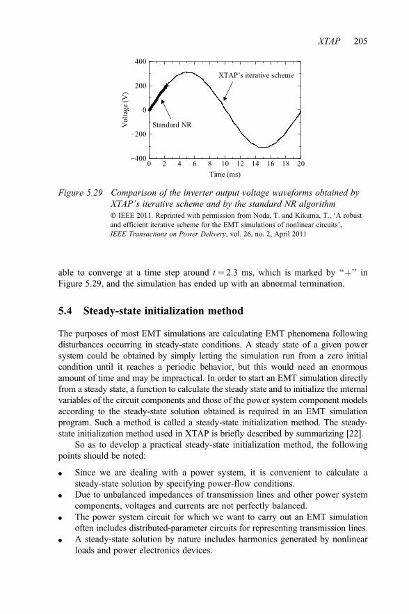
able to converge at a time step around t ¼ 2.3 ms, which is marked by ‘‘þ’’ inFigure 5.29, and the simulation has ended up with an abnormal termination.

5.4 Steady-state initialization method

The purposes of most EMT simulations are calculating EMT phenomena followingdisturbances occurring in steady-state conditions. A steady state of a given powersystem could be obtained by simply letting the simulation run from a zero initialcondition until it reaches a periodic behavior, but this would need an enormousamount of time and may be impractical. In order to start an EMT simulation directlyfrom a steady state, a function to calculate the steady state and to initialize the internalvariables of the circuit components and those of the power system component modelsaccording to the steady-state solution obtained is required in an EMT simulationprogram. Such a method is called a steady-state initialization method. The steady-state initialization method used in XTAP is briefly described by summarizing [22].

So as to develop a practical steady-state initialization method, the followingpoints should be noted:

● Since we are dealing with a power system, it is convenient to calculate asteady-state solution by specifying power-flow conditions.

● Due to unbalanced impedances of transmission lines and other power systemcomponents, voltages and currents are not perfectly balanced.

● The power system circuit for which we want to carry out an EMT simulationoften includes distributed-parameter circuits for representing transmission lines.

● A steady-state solution by nature includes harmonics generated by nonlinearloads and power electronics devices.

0 2 4 6 8 10 12 14 16 18 20−400

−200

0

200

400

Time (ms)

Vol

tage

(V)

XTAP’s iterative scheme

Standard NR

Figure 5.29 Comparison of the inverter output voltage waveforms obtained byXTAP’s iterative scheme and by the standard NR algorithm� IEEE 2011. Reprinted with permission from Noda, T. and Kikuma, T., ‘A robustand efficient iterative scheme for the EMT simulations of nonlinear circuits’,IEEE Transactions on Power Delivery, vol. 26, no. 2, April 2011

XTAP 205

Xia and Heydt proposed a method to solve circuit equations not only of thepower frequency but also of harmonic frequencies together with power-flow con-straints [23, 24]. In this pioneering work, only positive-sequence circuit equationsare taken into account, and thereby, unbalanced circuit conditions cannot berepresented. Later, methods to take both harmonics and unbalanced circuit condi-tions were proposed [25�27]. However, these methods simply calculate a steady-state solution by specifying the waveforms of voltage and current sources as thedriving force, not by specifying power-flow conditions as desired by power engi-neers. The methods proposed in [28�30] are able to take all of harmonics, unba-lanced circuit conditions, and power-flow constraints into account. If these methodsare viewed as steady-state initialization methods for EMT simulations, there isunfortunately the following intrinsic drawback. These methods are based on theshooting method [31]. Since the shooting method assumes that the circuit equationsare described by a set of ordinary differential equations (ODEs), distributed-parameter circuits which are described by partial differential equations (PDEs)cannot be included in the steady-state calculation [32].

Considering the discussion above, the three-stage method was proposed [22]and implemented in XTAP as its steady-state initialization function. The methodconsists of the following three stages:

Stage 1: Using power-flow conditions specified by the user, a conventional single-phase (positive-sequence) power-flow calculation is performed.

Stage 2: The generators and the substations connected to upper-voltage systemsincluded in the simulation circuit are replaced by balanced three-phasesinusoidal voltage sources whose magnitudes and phase angles areobtained by the power-flow solution of Stage 1. Then, a three-phasepower-frequency steady-state solution is calculated by solving the circuitequations in the frequency domain.

Stage 3: Based on the power-frequency steady-state solution obtained at Stage 2,the internal variables of the circuit components and those of the powersystem component models are initialized, and then, the EMT simulationis kept running for a certain number of cycles.

As an initial approximation, the conventional single-phase power-flow calcu-lation at Stage 1 gives a balanced power-frequency solution. Then, at Stage 2, thethree-phase power-frequency steady-state solution in the frequency domain takesinto account unbalanced circuit conditions at the power frequency. Finally, theEMT simulation at Stage 3 generates harmonics due to nonlinear loads and power-electronics devices. In this way, we can obtain a steady-state solution taking har-monics and unbalanced circuit conditions into account by specifying power-flowconditions.

The three-stage method should not be considered a novel method, and actually,most users of EMT simulation programs have been manually carrying out thesethree stages in their routine simulations. For details of the three stage method,consult [22].


5.5 Object-oriented design of the simulation code

The name XTAP stands for eXpandable Transient Analysis Program. The word‘‘eXpandable’’ comes from the fact that the simulation code of XTAP is written inthe Cþþ programming language and its design philosophy accepts adding a newsimulation model without substantial revision of the code. This topic is brieflyintroduced here by summarizing [33].

Power system engineers started using object-oriented methods for power sys-tem simulations in the late 1980s. Object-oriented methods are now used in variousaspects of power system simulations. In [34], an object-oriented implementation of aload-flow program using the Objective-C language is illustrated. How power systemcomponents such as transmission lines, transformers, etc. are modeled using classesis explained, and it is concluded that the object-oriented approach reduces the effortsof programming. Similar results are obtained in [35–37] using the Cþþ language.In addition, [35] shows how to handle sparse matrices using Cþþ, and [37] dealswith large-scale networks including FACTS controllers. Object-oriented modelingof a power system for dynamic stability-type simulations is proposed in [38] and forobtaining the steady-state solution of a nonlinear power network in [39], both usingCþþ. An object-oriented modeling methodology, called DCOM (DistributionCircuit Object Model), for a distribution analysis system is reported in [40]. As anapplication to other than programming, an object-oriented concept was used todevelop a common database which generates input data files for different simulationprograms ranging from load flow to electromagnetic transients [41]. The databasestores parameters of power system components in various aspects and appropriatelyprocesses the parameters to generate an input file for a specific type of power systemsimulations. Reference [42] reports a development of graphical user interfaces forpower system simulations using object-oriented programming. The development ofa fault locating system using an object-oriented approach is described in [43].

Two important features of the object-oriented programming are (i) abstractionof data and their procedures using ‘‘classes’’ and (ii) derivation of a new class froman existing class using the concept of ‘‘inheritance.’’ An efficient implementationof an electromagnetic transient program is reported in [44] based on a partly object-oriented approach using Fortran 95. The approach uses (i) for optimizing theexecution speed.

The core simulation code of XTAP is based on the following object-orienteddesign philosophy utilizing the Cþþ programming language. The object-orientedmethodology first defines a base class called ‘‘Branch’’ from which all kinds ofcircuit components are derived using inheritance. This is illustrated in Figure 5.30.The Branch class has data and their procedures which are common to all circuitcomponents but no specific model parameters and behaviors are defined. Usinginheritance, specific model parameters and behaviors are added to the Branch class,and as a result a specific circuit component is derived. From the Branch class, notonly simple components like resistors, inductors, capacitors, etc. but also complexcomponents such as a frequency-dependent line model are derived. In order to

XTAP 207

carry out an electromagnetic transient simulation, each circuit component has to beinitialized preceding the time step loop and then updated at each time step (if thecomponent is nonlinear, then updated at each iteration step). The design metho-dology significantly simplifies these processes. Since all circuit components arederived from the common base class Branch, all circuit components can be put intoan array of the Branch class. Once all components of a circuit are stored in thearray, the circuit solver can issue an initialization or updating message to eachelement of the array. When issuing these messages, the circuit solver does not haveto specify how to initialize or how to update and even does not have to know whateach element in the array is. On the other hand, each element knows how to initi-alize or update itself, since the initialization and updating processes are definedwhen each component has been derived from the Branch class. This enablesseparately writing the code of the circuit solver and that of circuit components andthus significantly simplifies the entire code structure. Code maintainability is alsoenhanced. Especially, adding a new component or a user-defined componentbecomes an easy task. When adding a new component, the circuit solver does nothave to be revised and only the code for deriving the new component from theBranch class is required. For details, consult [33].

References

[1] T. Noda, K. Takenaka, and T. Inoue, ‘‘Numerical integration by the 2-stagediagonally implicit Runge-Kutta method for electromagnetic transientsimulations,’’ IEEE Trans., Power Delivery, vol. 24, no. 1, pp. 390–399, Jan.2009.

Branch

VoltagesourceResistor Inductor Capacitor

Currentsource

Transm.line Generator

Nonlinearcapacitor

Nonlinearinductor

Nonlinearresistor Cable

Figure 5.30 Class hierarchy of the circuit components in the core simulation codeof XTAP� IPST 2011. Reprinted with permission from T. Noda and K. Takenaka, ‘A practicalsteady-state initialization method for electromagnetic transient simulations,’ Proc. ofIPST 2011, Paper # 11IPST097, Delft, The Netherlands, 2011


[2] H. W. Dommel, ‘‘Digital computer solution of electromagnetic transients insingle- and multi-phase networks,’’ IEEE Trans. Power Apparatus andSystems, vol. PAS-88, no. 4, pp. 388–399, Apr. 1969.

[3] U. M. Ascher and L. R. Petzold, ‘‘Computer Methods for Ordinary DifferentialEquations and Differential-Algebraic Equations,’’ SIAM, Philadelphia, PA,USA, 1998.

[4] J. R. Marti and J. Lin, ‘‘Suppression of numerical oscillations in the EMTP,’’IEEE Trans., Power Systems, vol. 4, no. 2, pp. 739–747, May 1989.

[5] J. Lin and J. R. Marti, ‘‘Implementation of the CDA procedure in theEMTP,’’ IEEE Trans., Power Systems, vol. 5, no. 2, pp. 394–402, May 1990.

[6] R. Alexander, ‘‘Diagonally implicit Runge-Kutta methods for stiff O.D.E.’s,’’SIAM Journal on Numerical Analysis, vol. 14, no. 6, pp. 1006–1021, Dec. 1977.

[7] C. W. Gear, Numerical Initial Value Problems in Ordinally DifferentialEquations, Prentice-Hall, Inc., NJ, USA, 1971.

[8] H. Shichman, ‘‘Integration system of a nonlinear network-analysis program,’’IEEE Trans., Circuit Theory, vol. CT-17, no. 3, pp. 378–386, Aug. 1970.

[9] A. Prothero and A. Robinson, ‘‘On the stability and accuracy of one-stepmethods for solving stiff systems of ordinary differential equations,’’ Math.Comp., vol. 28, pp. 145–162, 1974.

[10] T. Noda, T. Kikuma, and R. Yonezawa, ‘‘Supplementary techniques for2S-DIRK-based EMT simulations,’’ Electric Power Systems Research,Elsevier, Vol. 115, pp. 87–93, Oct. 2014. See http://www.sciencedirect.com/science/article/pii/S0378779614001515.

[11] T. Noda and T. Kikuma, ‘‘A robust and efficient iterative scheme for theEMT simulations of nonlinear circuits,’’ IEEE Trans., Power Delivery,vol. 26, no. 2, pp. 1030–1038, Apr. 2011.

[12] L. O. Chua, ‘‘Efficient computer algorithms for piecewise-linear analysis ofresistive nonlinear networks,’’ IEEE Trans., Circuit Theory, vol. CT-18,no. 1, pp. 73–85, Jan. 1971.

[13] J. Katzenelson, ‘‘An algorithm for solving nonlinear resistor networks,’’Bell Syst. Tech. J., vol. 44, no. 8, pp. 1605–1620, Oct. 1965. See http://onlinelibrary.wiley.com/doi/10.1002/j.1538-7305.1965.tb04195.x/abstract.

[14] T. Fujisawa and E. S. Kuh, ‘‘Piecewise-linear theory of nonlinear networks,’’SIAM J. Appl. Math., vol. 22, no. 2, pp. 307–328, Mar. 1972.

[15] T. Ohtsuki, T. Fujisawa, and S. Kumagai, ‘‘Existence theorems and a solu-tion algorithm for piecewise-linear resistor networks,’’ SIAM J. Math. Anal.,vol. 8, no. 1, pp. 69–99, Feb. 1977.

[16] L. O. Chua and P.-M. Lin, Computer-Aided Analysis of Electronic Circuits—Algorithms and Computational Techniques, Prentice-Hall, EnglewoodCliffs, NJ, USA, 1975.

[17] C.-W. Ho, A. E. Ruehli, and P. A. Brennan, ‘‘The modified nodal approachto network analysis,’’ IEEE Trans., Circuit and Systems, vol. CAS-22, no. 6,pp. 504–509, Jun. 1975.

[18] G. D. Hachtel, R. K. Brayton, and F. G. Gustavson, ‘‘The sparse tableauapproach to network analysis and design,’’ IEEE Trans., Circuit Theory,vol. CT-18, no. 1, pp. 101–113, Jan. 1971.

XTAP 209

[19] R. A. Rohrer, Circuit Theory: An introduction to the state variableapproach, McGraw-Hill, Englewood Cliffs, NJ, USA, 1975.

[20] T. Kikuma, N. Okada, M. Takasaki, A. Kuzumaki, and K. Kodani, ‘‘Simu-lation analysis of SiC diode applied inverter,’’ Proc., 2008 IEEJ IndustryApplications Society Conference, pp. I 347–350, 2008 (in Japanese).

[21] R. Kraus, P. Turkes, and J. Sigg, ‘‘Physics-based models of power semi-conductor devices for the circuit simulator SPICE,’’ Proc., 29th AnnualIEEE Power Electronics Specialists Conference Record, vol. 2,pp. 1726–1731, May 1998.

[22] T. Noda and K. Takenaka, ‘‘A practical steady-state initialization method forelectromagnetic transient simulations,’’ Proc. of IPST 2011, Paper #11IPST097, Delft, The Netherlands, 2011.

[23] D. Xia and G. T. Heydt, ‘‘Harmonic power flow studies Part I—Formulationand solution,’’ IEEE Trans., Power Apparatus and Systems, vol. 101, no. 6,pp. 1257–1265, Jun. 1982.

[24] D. Xia and G. T. Heydt, ‘‘Harmonic power flow studies Part II—Imple-mentation and practical application,’’ IEEE Trans., Power Apparatus andSystems, vol. 101, no. 6, pp. 1266–1270, Jun. 1982.

[25] A. Semlyen and A. Medina, ‘‘Computation of the periodic steady state insystems with nonlinear components using a hybrid time and frequencydomain methodology,’’ IEEE Trans., Power Systems, vol. 10, no. 3,pp. 1498–1504, Aug. 1995.

[26] E. Acha and M. Madrigal, Power Systems Harmonics: Computer Modellingand Analysis, 1st edition, John Wiley & Sons, Ltd, West Sussex, EnglandJun. 4, 2001.

[27] T. Noda, A. Semlyen, and R. Iravani, ‘‘Entirely harmonic domain calculationof multiphase nonsinusoidal steady state,’’ IEEE Trans., Power Delivery,vol. 19, no. 3, pp. 1368–1377, Jul. 2004.

[28] A. Semlyen and M. Shlash, ‘‘Principles of modular harmonic power flowmethodology,’’ IEE Proceedings—Generation, Transmission and Distribu-tion, vol. 147, no. 1, pp. 1–6, Jan. 2000.

[29] N. Garcia and E. Acha, ‘‘Periodic steady-state analysis of large-scale electricsystems using Poincare map and parallel processing,’’ IEEE Trans., PowerSystems, vol. 19, no. 4, pp. 1784–1793, Nov. 2004.

[30] K. L. Lian and T. Noda, ‘‘A time-domain harmonic power-flow algorithmfor obtaining nonsinusoidal steady-state solutions,’’ IEEE Trans., PowerDelivery, vol. 25, no. 3, pp. 1888–1898, Jul. 2010.

[31] T. J. Aprille and T. N. Trick, ‘‘Steady state analysis of nonlinear circuits withperiodic inputs,’’ Proceedings of the IEEE, vol. 60, no. 1, pp. 108–114, Jan.1972. See http://ieeexplore.ieee.org/xpl/login.jsp?tp=&arnumber=1450493&url=http%3A%2F%2Fieeexplore.ieee.org%2Fxpls%2Fabs_all.jsp%3Farnumber%3D1450493

[32] K. S. Kundert, ‘‘Steady-state methods for simulating analog circuits,’’ Ph.D.Thesis, University of California, Berkley, Technical Report No. UCB/ERLM89/63, 1989.


[33] T. Noda, ‘‘Object oriented design of a transient analysis program,’’ Proc. ofIPST 2011, Paper # 07IPST075, Lyon, France, 2007.

[34] A. F. Neyer, F. F. Wu, and K. Imhof, ‘‘Object-oriented programming forflexible software: Example of load flow,’’ IEEE Trans. on Power Systems,vol. 5, no. 3, pp. 689–696, Aug. 1990.

[35] B. Hakavik and A. T. Holen, ‘‘Power system modeling and sparse matrixoperations using object-oriented programming,’’ IEEE Trans. on PowerSystems, vol. 9, no. 2, pp. 1045–1051, May 1994.

[36] E. Z. Zhou, ‘‘Object-oriented programming, Cþþ and power system simu-lation,’’ IEEE Trans. on Power Systems, vol. 11, no. 1, pp. 206–215, Feb.1996.

[37] C. R. Fuerte-Esquivel, E. Acha, S. G. Tan, and J. J. Rico, ‘‘Efficient objectoriented power systems software for the analysis of large-scale networkscontaining FACTS-controlled branches,’’ IEEE Trans. on Power Systems,vol. 13, no. 2, pp. 464–472, May 1998.

[38] A. Manzoni, A. S. e Silva, and I. C. Decker, ‘‘Power system dynamicssimulation using object-oriented programming,’’ IEEE Trans. on PowerSystems, vol. 14, no. 1, pp. 249–255, Feb. 1999.

[39] A. Medina, A. Ramos-Paz, R. Mora-Juarez, and C. R. Fuerte-Esquivel,‘‘Object oriented programming techniques applied to conventional and fasttime domain algorithms for the steady state solution of nonlinear electricnetworks,’’ Proc. 2004 IEEE Power Engineering Society General Meeting,pp. 342–346, Jun. 6–10, 2004.

[40] J. Zhu and D. L. Lubkeman, ‘‘Object-oriented development of softwaresystems for power system simulations,’’ IEEE Trans. on Power Systems, vol.12, no. 2, pp. 1002–1007, May 1997.

[41] D. G. Flinn and R. C. Dugan, ‘‘A database for diverse power systemsimulation applications,’’ IEEE Trans. on Power Systems, vol. 7, no. 2,pp. 784–790, May 1992.

[42] M. Foley, W. Mitchell, and A. Faustini, ‘‘An object based graphical userinterface for power systems,’’ IEEE Trans. on Power Systems, vol. 8, no. 1,pp. 97–104, Feb. 1993.

[43] M. Kezunovic and Y. Liao, ‘‘Development of a fault locating system usingobject-oriented programming,’’ Proc. 2001 IEEE ower Engineering SocietyWinter Meeting, pp. 763–768, Jan. 28–Feb. 1, 2001.

[44] J. Mahseredjian, B. Bressac, A. Xemard, L. Gerin-Lajoie, and P.-J. Lagace,‘‘A Fortran-95 implementation of EMTP algorithms,’’ Proc. of IPST 2001,Paper # 01IPST118, Rio de Janeiro, Brazil, 2001.

XTAP 211

Chapter 6

Numerical electromagnetic analysisusing the FDTD method

Y. Baba*

6.1 Introduction

Numerical electromagnetic analysis (NEA) methods, which include the method ofmoments (MoM) [1], the finite-element method (FEM) [2], the partial-elementequivalent-circuit (PEEC) method [3], the hybrid electromagnetic/circuit model(HEM) [4], the transmission-line-matrix (TLM) method [5], and the finite-differencetime-domain (FDTD) method [6], have been widely used in analyzing lightningelectromagnetic pulses (LEMPs) and surges (e.g., [7–11]). One of the advantages ofNEA, in comparison with circuit simulation methods, is that it allows a self-consistent full-wave solution for both the transient current distribution in a 3Dconductor system and resultant electromagnetic fields, although they are computa-tionally expensive.

Among NEA methods, the FDTD method has been most frequently used inLEMP calculations. The first peer-reviewed paper, in which the FDTD method wasused in a lightning electromagnetic field simulation, was published in 2003 byBaba and Rakov [12], and it was first applied to the surge analysis of groundingelectrodes by Tanabe [13] in 2001. The amount of published material on applica-tions of the FDTD method to lightning electromagnetic field and surge simulationsis quite large. Interest in using the FDTD method continues to grow because of theavailability of numerical codes and increased computer capabilities.

In this chapter, applications of the FDTD method to lightning electro-magnetic field and surge simulations are reviewed. The structure of this chapter isas follows. In section 6.2, the fundamental theory of the FDTD method is brieflydescribed, and advantages and disadvantages of the FDTD method in comparisonwith other representative NEA methods are identified. In section 6.3, sevenrepresentations of the lightning return-stroke channel used to date are described.In section 6.4, representative applications of the FDTD method are reviewed.They include simulations of (i) lightning electromagnetic fields at close and fardistances [12, 14–30], (ii) lightning surges on overhead power transmission lines

*Doshisha University, Japan

and towers [31–41], (iii) lightning surges on overhead power distribution lines[42–50], (iv) lightning electromagnetic environment in power substations [51],(v) lightning electromagnetic environment in airborne vehicles [52, 53],(vi) lightning surges and electromagnetic environment in buildings [54–58], and(vii) surges on grounding electrodes [13, 59–65].

6.2 FDTD method

6.2.1 FundamentalsThe FDTD method involves the space and time discretization of the working spaceand the finite-difference approximation to Maxwell’s equations. For the analysisof the electromagnetic response of a structure in an unbounded space using theFDTD method, an absorbing boundary condition such as Liao’s condition [66] orperfectly matched layers [67], which suppress unwanted reflections, should beapplied.

The method requires the whole working space to be divided into cubic orrectangular cells. Cells for specifying or computing electric field (electric fieldcells) and magnetic field cells are placed relative to each other as shown inFigure 6.1. Generally, the cell size (Dx, Dy, and Dz) should not exceed one-tenthof the wavelength corresponding to the highest frequency in the excitation.Time-updating equations for electric- and magnetic-field components, Ex, Ey, Ez,Hx, Hy, and Hz, are derived and as shown below.

Ampere’s law is given as

r�Hn�12 ¼ e

@En�12

@tþ Jn�1

2 ¼ e@En�1

2

@tþ sEn�1

2 ð6:1Þ

where H is the magnetic field intensity vector, E is the electric field intensityvector, J is the conduction-current-density vector, e is the electric permittivity, s is

H-field cell

Δz

Δx

ΔyEz(i, j, k+1/2)

Hx(i, j-1/2, k+1/2)

Hx(i, j+1/2, k+1/2)

Hy(i+1/2, j, k+1/2)

Hy(i–1/2, j, k+1/2)

E-field cell

Ez(i, j–1, k+1/2)

Ez(i, j, k+1/2)

Ey(i, j–1/2, k+1)

Ey(i, j–1/2, k)

Hx(i, j–1/2, k+1/2)

E-field cell

H-field cell

Figure 6.1 Placement of electric-field and magnetic-field cells for solvingdiscretized Maxwell’s equations using the FDTD method


the electric conductivity, t is the time, and n � 1/2 is the present time step. If thetime-derivative term in (6.1) is approximated by its central finite difference, (6.1)can be expressed as

e@En�1

2

@tþ sEn�1

2 � eEn � En�1

Dtþ s

En þ En�1

2� r�Hn�1

2 ð6:2Þ

where Dt is the time increment. Note that En�1/2 in the second term of (6.2) isapproximated by its average value, (En þ En�1)/2. Rearranging (6.2), the updatingequation for electric field at time step n from its one time-step previous value En�1

and half time-step previous magnetic-field curl value r�Hn�1=2 is obtained asfollows:

En ¼1 � sDt

2e

1 þ sDt

2e

0B@

1CAEn�1 þ

Dt

e

1 þ sDt

2e

0B@

1CAr�Hn�1

2 ð6:3Þ

From (6.3), the updating equation for Ezn at the space point (i þ 1/2, j, k) (see,

e.g., Figure 6.1) is expressed as

Enz i; j; k þ 1

2

� �¼

1 � sði; j; k þ 1=2ÞDt

2eði; j; k þ 1=2Þ1 þ sði; j; k þ 1=2ÞDt

2eði; j; k þ 1=2ÞEn�1

z i; j; k þ 12

� �

þDt

eði; j; k þ 1=2Þ1 þ sði; j; k þ 1=2ÞDt

2eði; j; k þ 1=2Þ

@Hn�1

2y i; j; k þ 1

2

� �@x

�@H

n�12

x i; j; k þ 12

� �@y

2664

3775

�1 � sði; j; k þ 1=2ÞDt

2eði; j; k þ 1=2Þ1 þ sði; j; k þ 1=2ÞDt

2eði; j; k þ 1=2ÞEn�1

z i; j; k þ 12

� �þ

Dt

eði; j; k þ 1=2Þ1 þ sði; j; k þ 1=2ÞDt

2eði; j; k þ 1=2Þ

1DxDy

�H

n�12

y i þ 12; j; k þ 1

2

� �Dy � H

n�12

y i � 12; j; k þ 1

2

� �Dy

�Hn�1

2x i; j þ 1

2; k þ 1

2

� �Dx þ H

n�12

x i; j � 12; k þ 1

2

� �Dx

266664

377775

ð6:4Þwhere the spatial-derivative terms in (6.4) are approximated by their central finitedifferences. Updating equations for En

x and Eny can be derived in the same manner.

Numerical electromagnetic analysis using the FDTD method 215

Faraday’s law is written as

r� En ¼ �m@Hn

@tð6:5Þ

where n is the present time step and m is the magnetic permeability. If the time-derivative term in (6.5) is approximated by its central finite difference, (6.5) isexpressed as

m@Hn

@t� m

Hnþ12 �Hn�1

2

Dt� �r� En ð6:6Þ

Rearranging (6.6), we obtain the updating equation for magnetic field at timestep n þ 1/2 from its one time-step previous value Hn�1/2 and half time-step pre-vious electric-field curl value r� En as follows:

Hnþ1=2 ¼ Hn�1=2 � Dt

mr� En ð6:7Þ

From (6.7), the updating equation for Hxnþ1/2 at the location (i, j � 1/2, k þ 1/2)

(see, e.g., Figure 6.1) is expressed as follows:

Hnþ1

2x i; j � 1

2; k þ 1

2

� �¼ H

n�12

x i; j � 12; k þ 1

2

� �þ Dt

m i; j � 1=2; k þ 1=2ð Þ

� �@En

z i; j � 12; k þ 1

2

� �@y

þ@En

y i; j � 12; k þ 1

2

� �@z

2664

3775

� Hn�1

2x i; j � 1

2; k þ 1

2

� �þ Dt

m i; j � 1=2; k þ 1=2ð Þ1

DyDz

��En

z i; j; k þ 12

� �Dz þ En

z i; j � 1; k þ 12

� �Dz

þEny i; j � 1

2; k þ 1

� �Dy � En

y i; j � 12; k

� �Dy

26664

37775ð6:8Þ

where the spatial-derivative terms in (6.8) are approximated by their central finitedifferences. Updating equations for Hnþ1=2

y and Hnþ1=2z can be derived in the same

manner.By updating En

x , Eny , En

z , Hnþ1=2x , Hnþ1=2

y , and Hnþ1=2z at every point, transient

electric and magnetic fields throughout the working volume are obtained.


6.2.2 Advantages and disadvantagesAdvantages of the FDTD method in comparison with other NEA methods aresummarized as follows:

1. It is based on a simple procedure in electric and magnetic field computations,and therefore its programming is relatively easy.

2. It is capable of treating complex geometries and inhomogeneities.3. It is capable of incorporating nonlinear effects and components.4. It can handle wideband quantities from one run with the help of a time-to-

frequency transforming tool.

Disadvantages are as follows:

1. It is computationally expensive compared to other methods such as theMoM.

2. It cannot deal with oblique boundaries that are not aligned with the Cartesiangrid.

3. It would require a complex procedure for incorporating dispersive materials.

6.3 Representations of lightning return-stroke channelsand excitations

6.3.1 Lightning return-stroke channelsSeven types of representation of lightning return-stroke channels are used in elec-tromagnetic pulse and surge computations:

1. a perfectly conducting/resistive wire in air above ground;2. a wire loaded by additional distributed series inductance in air above

ground;3. a wire surrounded by a dielectric medium (other than air) that occupies the

entire half space above ground (this fictitious configuration is used only forfinding current distribution, which is then applied to a vertical wire in air aboveground for calculating electromagnetic fields);

4. a wire coated by a dielectric material in air above ground;5. a wire coated by a fictitious material having high relative permittivity and high

relative permeability in air above ground;6. two parallel wires having additional distributed shunt capacitance in air (this

fictitious configuration is used only for finding current distribution, which isthen applied to a vertical wire in air above ground for calculating electro-magnetic fields); and

7. a phased-current-source array in air above ground, each current source beingactivated successively by the arrival of lightning return-stroke wavefront pro-gressing upward at a specified speed.


The return-stroke speed, along with the current peak, largely determines theradiation field initial peak (e.g., [68]). The characteristic impedance of the lightningreturn-stroke channel influences the magnitude of lightning current and/or thecurrent reflection coefficient at the top of the strike object when a lumped voltagesource is employed. It is therefore desirable that the return-stroke speed and thecharacteristic impedance of simulated lightning channel agree with observationsthat can be summarized as follows:

1. Typical values of return-stroke speed are in the range from c/3 to c/2 [69], asobserved using optical techniques, where c is the speed of light.

2. The equivalent impedance of the lightning return-stroke channel is expected tobe in the range from 0.6 to 2.5 kW [70].

Type 1 was used, for example, by Baba and Rakov [12] in their FDTD simu-lation on electromagnetic fields due to a lightning strike to flat ground. Note thatthis lightning-channel representation was first used by Podgorski and Landt [71] intheir simulation of lightning current in a tall structure with the MoM in the timedomain. The speed of the current wave propagating along a vertical perfectlyconducting/resistive wire is nearly equal to the speed of light, which is two tothree times larger than typical measured values of return-stroke wavefront speed(c/3 to c/2). This discrepancy is the main deficiency of this representation. Thecharacteristic impedance of the channel-representing vertical wire of radius 3 cm isestimated to be around 0.6 kW at a height of 500 m above ground (it varies withheight above ground). This is right at the lower bound of its expected range ofvariation (0.6 to 2.5 kW). Note that a current wave suffers attenuation (distortion)as it propagates along a vertical wire even if it has no ohmic losses [31].Further attenuation can be achieved by loading the wire by distributed seriesresistance.

Type 2 was used, for example, by Baba and Rakov [7] in their FDTD simu-lation of current along a vertical lightning channel. Note that this lightning-channel representation was first used by Kato et al. [72] in their simulation onlightning current in a tall structure and its associated electromagnetic fields withthe MoM in the time domain. The speed of the current wave propagating along avertical wire loaded by additional distributed series inductance of 17 and 6.3 mH/min air is c/3 and c/2, respectively, if the natural inductance of vertical wire isassumed to be L0 ¼ 2.1 mH/m (as estimated by Rakov [73] for a 3-cm-radius wireat a height of 500 m above ground). The corresponding characteristic impedanceranges from 1.2 to 1.8 kW (0.6 kW� [(17 þ 2.1)/2.1]1/2 ¼ 1.8 kW, and 0.6 kW�[(6.3 þ 2.1)/2.1]1/2 ¼ 1.2 kW) for the speed ranging from c/3 to c/2. The char-acteristic impedance of the inductance-loaded wire is within the range of values ofthe expected equivalent impedance of the lightning return-stroke channel. Note thatadditional inductance has no physical meaning and is invoked only to reduce thespeed of current wave propagating along the wire to a value lower than the speed oflight. The use of this representation allows one to calculate both the distributionof current along the channel-representing wire and remote electromagnetic fields in


a single, self-consistent procedure. Bonyadi-ram et al. [74] have incorporatedadditional distributed series inductance that increases with increasing height inorder to simulate the optically observed reduction in return-stroke speed withincreasing height (e.g., [75]).

Type 3 was used, for example, by Baba and Rakov [7] in their FDTDsimulation of current along a vertical lightning channel. Note that this lightning-channel representation was first used by Moini et al. [76] in their simulation onlightning electromagnetic fields with the MoM in the time domain. The artificialdielectric medium was used only for finding current distribution along thelightning channel, which was then removed for calculating electromagneticfields in air. When the relative permittivity is 9 or 4, the speed is c/3 or c/2,respectively. The corresponding characteristic impedance ranges from 0.2 to0.3 kW (0.6 kW/

ffiffiffi9

p ¼ 0.2 kW, and 0.6 kW/ffiffiffi4

p ¼ 0.3 kW) for the speed rangingfrom c/3 to c/2. These characteristic impedance values are smaller than theexpected ones (0.6 to 2.5 kW).

Type 4 was used, for example, by Baba and Rakov [7] in their FDTD simu-lation of current along a vertical lightning channel. Note that this lightning-channelrepresentation was first used by Kato et al. [77] in their simulation of lightningelectromagnetic fields with the MoM in the frequency domain. Baba and Rakov [7]represented the lightning channel by a vertical perfectly conducting wire, whichhad a radius of 0.23 m and was placed along the axis of a dielectric rectangularparallelepiped of relative permittivity 9 and cross section 4 m � 4 m. This dielectricparallelepiped was surrounded by air. The speed of the current wave propagatingalong the wire was about 0.74c. Such a representation allows one to calculate boththe distribution of current along the wire and the remote electromagnetic fields in asingle, self-consistent procedure, while that of a vertical wire surrounded by anartificial dielectric medium occupying the entire half space (type 3 describedabove) requires two steps to achieve the same objective. However, the electro-magnetic fields produced by a dielectric-coated wire in air might be influenced bythe presence of coating.

Type 5 was first used by Miyazaki and Ishii [78] in their FDTD simulation ofelectromagnetic fields due to a lightning strike to a tall structure. Although theexact values of relative permittivity and relative permeability of the coating werenot given in [78], the speed of the current wave propagating along the wire wasabout 0.5c. Similar to type 4, this representation allows one to calculate both thedistribution of current along the wire and the remote electromagnetic fields in asingle, self-consistent procedure. For the same speed of current wave, the char-acteristic impedance value for this channel representation is higher than that fortype 4, since both relative permittivity and permeability are set at higher values inthe type 5 representation.

Type 6 has not been used in LEMP and surge simulations with the FDTDmethod to date. It was, however, used by Bonyadi-ram et al. [79] in their simulationwith the MoM in the time domain. The speed of the current wave propagating alongtwo parallel wires having additional distributed shunt capacitance in air is 0.43cwhen the additional capacitance is 50 pF/m. In this model, each of the wires has a


radius of 2 cm, and the separation between the wires is 30 m. Similar to type 3described above, this representation employs a fictitious configuration for finding areasonable distribution of current along the lightning channel, and then this currentdistribution is applied to the actual configuration (vertical wire in air aboveground).

Type 7 was used by Baba and Rakov [12] in their FDTD calculations oflightning electromagnetic fields. This representation can be employed for simula-tion of ‘‘engineering’’ lightning return-stroke models. Each current source of thephased-current-source array is activated successively by the arrival of lightningreturn-stroke wavefront that progresses upward at a specified speed. Although theimpedance of this channel model is infinity, appropriate reflection coefficients atthe top and bottom of the structure and at the lightning attachment point can bespecified to account for the presence of tall strike object and upward-connectingleader (e.g., [80, 81]).

Among the above seven types, types 2 and 5 appear to be best in terms ofthe resultant return-stroke wavefront speed, the characteristic impedance, and theprocedure for current and field computations. Type 7 is also useful since thereturn-stroke wavefront speed and the current attenuation with height are con-trolled easily with a simple mathematical expression: ‘‘engineering’’ return-strokemodel such as the transmission-line (TL) model [82], the traveling-current-source(TCS) model [83], or the modified transmission-line model with linear currentdecay model with linear current decay (MTLL) model [68].

6.3.2 ExcitationsMethods of excitation of the lightning channel used in electromagnetic pulse andsurge computations include:

1. closing a charged vertical wire at its bottom end with a specified impedance(or circuit);

2. a lumped voltage source (same as a delta-gap electric-field source);3. a lumped current source; and4. a phased-current-source array.

Type 1 was used, for example, by Baba and Rakov [7] in their FDTD simu-lation of currents along a vertical lightning channel. Note that this representationwas first used by Podgorski and Landt [71] in their simulation of lightning currentswith the MoM in the time domain. Baba and Rakov [7] represented a leader/return-stroke sequence by a pre-charged vertical perfectly conducting wire connected viaa nonlinear resistor to flat ground. In their model, closing a charged vertical wire ina specified circuit simulates the lightning return-stroke process.

Type 2 representation was used, for example, by Baba and Rakov [7] in theirFDTD simulation of lightning currents, but it was first used by Moini et al. [84] intheir simulation of lightning-induced voltages with the MoM in the time domain.This type of source generates a specified electric field, which is independent of


current flowing through the source. Since it has zero internal impedance, its pre-sence in series with the lightning channel and strike object does not disturb anytransient processes in them. If necessary, one could insert a lumped resistor inseries with the voltage source to adjust the impedance seen by waves entering thechannel from the strike object to a value consistent with the expected equivalentimpedance of the lightning channel.

Type 3 was used, for example, by Noda et al. [33]. However, in contrast witha lumped voltage source, a lumped current source inserted at the attachmentpoint is justified only when reflected waves returning to the current source arenegligible. This is the case for a branchless subsequent lightning strike termi-nating on flat ground, in which case an upward connecting leader is usuallyneglected and the return-stroke current wave is assumed to propagate upwardfrom the ground surface. The primary reason for the use of a lumped currentsource at the channel base is a desire to use directly the channel-base current,known from measurements for both natural and triggered lightning, as an inputparameter of the model. When one employs a lumped ideal current source at theattachment point in analyzing lightning strikes to a tall grounded object, thelightning channel, owing to the infinitely large impedance of the ideal currentsource, is electrically isolated from the strike object, so that current wavesreflected from ground cannot be directly transmitted to the lightning channel(only electromagnetic coupling is possible). Since this is physically unreason-able, a series ideal current source is not suitable for modeling of lightning strikesto tall grounded objects [80].

Features of type 4 excitation are described in section 6.3.1 for type 7 repre-sentation of lightning return-stroke channel.

6.4 Applications

In this section, representative applications of the FDTD method are reviewed.These include simulations of (i) lightning electromagnetic fields at close and fardistances [12, 14–30], (ii) lightning surges on overhead power transmission linesand towers [31–41], (iii) lightning surges on overhead power distribution lines[42–50], (vi) lightning electromagnetic environment in power substations [51],(v) lightning electromagnetic environment in airborne vehicles [52, 53], (vi) light-ning surges and electromagnetic environment in buildings [54–58], and (vii) surgeson grounding electrodes [13, 59–65].

6.4.1 Lightning electromagnetic fields at close andfar distances

The FDTD method has been widely used in analyzing electromagnetic fields due tolightning strikes to flat ground. When the lightning channel is vertical andthe configuration is cylindrically symmetrical, simulations are often performed inthe 2D cylindrical coordinate system (e.g., [14, 15, 18–20, 23, 25, 29, 30]), since


2D simulations are computationally much less expensive than the corresponding3D simulations. Since the FDTD method yields reasonably accurate results forlossy ground, it has been used to test the validity of approximate expressions forhorizontal electric fields [14, 23, 24] such as the Cooray-Rubinstein formula [85].Also, underground electric and magnetic fields have been analyzed by Mimouniet al. [29]. Furthermore, the influence of horizontally stratified ground has beenstudied by Shoory et al. [20] and Zhang et al. [27], and the influence of roughground surface has been investigated by Li et al. [26, 28].

Baba and Rakov [17] have calculated, using the 3D FDTD method, the ver-tical electric field Ez and azimuthal magnetic field Hj due to lightning strikesin the presence and in the absence of building at the field point, as shown inFigure 6.2. Strikes to both flat ground and tall objects of height h ¼ 100, 200, or500 m were considered, and the strike object and the lightning current wererepresented by a vertical array of current sources specified using the ‘‘engineer-ing’’ TL model as described by Baba and Rakov [86]. The magnitude of Hj is notmuch influenced by the presence of either building at the field point or strikeobject, while the magnitude of Ez is significantly influenced by either of them. Inthe case of a lightning strike to flat ground, the magnitude of Ez at the top of thebuilding (at the center point of its flat roof) of plan area Sb ¼ 40 m � 40 m andheight hb ¼ 20, 50, or 100 m located at a horizontal distance d ranging from 100 to500 m from the lightning channel is about 1.5, 2, or 3 times, respectively, greaterthan that at the same horizontal distance on the ground surface in the absence ofbuilding, as shown in Table 6.1. The magnitude of Ez at ground level in theimmediate vicinity of the building is reduced relative to the case of no building,with this shielding effect becoming negligible at horizontal distances from thebuilding exceeding twice the height of the building. The ratios for lightningstrikes to a tall object of height 100, 200, or 500 m are almost the same as those inthe case of lightning strike to flat ground, although the corresponding results arenot shown here. On the basis of these results, Nag et al. [87] employed an electricfield enhancement factor of 1.4 for their antenna installed on the roof of a five-story building.

Berenger [15] has analyzed Ez radiated by a lightning strike at a distance of morethan 5,000 km on the flat Earth surface using the 2D cylindrical FDTD method. Herepresents lightning channel by a 1 km vertical current dipole, and uses a 1,000-km-longdomain that moved horizontally and was divided into 0.5 km� 0.5 km squarecells. Oikawa et al. [21] have carried out a similar simulation of Ez using the 3DFDTD method. They represent lightning channel as a 10 m vertical current source,simulate a realistic bumpy ground geometry with 10 m � 10 m � 10 m cubiccells, and employ a 7 km � 4 km� 7 km moving domain within a 7 km �28 km� 7 km working volume. Haddad et al. [22] computed vertical electric fieldwaveforms at distances ranging from 100 to 400 km using an FDTD model ofVLF propagation in the Earth-ionosphere waveguide [16].

Using the 2D cylindrical FDTD method, Baba and Rakov [18] have calculatedEz, horizontal (radial) electric field Eh, and Hj produced on the ground surface bylightning strikes to a 160 m and a 553 m high conical strike objects representing the


1,000 m

1,000 m

TLs representingchannel and strike object

Building

d = 100, 200, or 500 m

Points 1, 2, and 3

Liao’s 2nd-order absorbing boundaries

1,000 m 1,500 m

Plan view

2,700 m

300 m

TL representingstrike object

Buildinghb = 0, 20, 50, or 100 m

Points 1, 2, and 3

TL representingchannel

v = 0.5c

h = 0, 100, 200, or 500 m

sb = 1 mS/m, erb = 10

sg = 1 mS/m, erg = 10

1,000 m 1,500 m

Side view

Figure 6.2 Building of height hb ¼ 0 (for the case of no building), 20, 50, or 100 mand plan area Sb ¼ 40 m � 40 m located at distance d ¼ 100, 200, or500 m from a tall grounded object of height h ¼ 0 (for the case oflightning strike to flat ground), 100, 200, or 500 m struck by lightning.The strike object and the lightning channel are represented by avertical array of current sources specified using the ‘‘engineering’’TL model described by Baba and Rakov [86]. The current propagationspeed along the lightning channel is set to v ¼ 0.5c. The workingvolume of 2,000 m � 2,500 m � 3,000 m is divided into 10 m �10 m � 10 m cubic cells and surrounded by six planes of Liao’ssecond-order absorbing boundary condition [66] to avoid reflectionsthere� 2007 IEEE. Reprinted with permission from Yoshihiro Baba and Vladimir A. Rakov,‘Electromagnetic fields at the top of a tall building associated with nearby lightningreturn strokes’, IEEE Transactions on Electromagnetic Compatibility, vol. 49, no. 3,pp. 632–643, August 2007, Figure 1


Peissenberg tower (Germany) and the CN Tower (Canada), respectively. The fieldsare computed for a typical subsequent stroke at distances d 0 from the bottom of theobject ranging from 5 to 100 m for the 160 m tower and from 10 to 300 m forthe 553 m tower. Grounding of the 160 m object is assumed to be accomplished byits underground basement represented by a 10-m-radius and 8-m-long perfectlyconducting cylinder with or without a reference ground plane located 2 m below.The reference ground plane simulates, to some extent, a higher conducting groundlayer that is expected to exist below the water table. The configuration withoutreference ground plane actually means that this plane is present, but is located at aninfinitely large depth. Grounding of the 553 m object is modeled in a similarmanner but in the absence of reference ground plane only. In all cases considered,waveforms of Eh and Hj are not much influenced by the presence of strike object,while waveforms of Ez are. Waveforms of Ez are essentially unipolar (as they are inthe absence of strike object) when the ground conductivity s is 10 mS/m (theequivalent transient impedance is several ohm) or greater. For the 160 m tower andfor s¼ 1 and 0.1 mS/m, waveforms of Ez become bipolar (exhibit polarity change)at d 0 � 10 m and d 0 � 50 m, respectively, regardless of the presence of thereference ground plane. The corresponding equivalent transient grounding impe-dances are about 30 and 50 W in the absence of the reference ground plane andsmaller than 10 W in the presence of the reference ground plane. The source ofopposite polarity Ez is the potential rise at the object base (at the air/ground inter-face) relative to the reference ground plane. For a given grounding electrode geo-metry, the strength of this source increases with decreasing s, provided that the

Table 6.1 Ratios of magnitudes of vertical electric field Ez at points 1, 2, and 3(see Figure 6.2) due to a lightning strike to flat ground (h ¼ 0) in thepresence of building of height hb ¼ 20, 50, and 100 m at the field point,located at a horizontal distance of d ¼ 100, 200, and 500 m from thelightning strike point and those in the absence of building (hb ¼ 0)

Field point Horizontaldistance, d (m)

Building height, hb (m)

20 50 100

Point 1, on ground in front of building 100 0.98 0.94 0.88200 0.95 0.88 0.77500 0.96 0.82 0.71

Point 2, on roof of building 100 1.5 2.1 2.7200 1.5 2.2 3.0500 1.5 2.2 3.2

Point 3, on ground behind building 100 0.90 0.69 0.46200 0.91 0.72 0.51500 0.93 0.75 0.57

� 2007 IEEE. Reprinted with permission from Yoshihiro Baba and Vladimir A. Rakov, ‘Electro-magnetic fields at the top of a tall building associated with nearby lightning return strokes’, IEEETransactions on Electromagnetic Compatibility, vol. 49, no. 3, pp. 632–643, August 2007, Table I.


grounding impedance is linear. Potential rises at the strike object base for s¼ 1 and0.1 mS/m are some hundreds of kilovolts, which is sufficient to produce electricalbreakdown from relatively sharp edges of the basement over a distance of severalmeters (or more) along the ground surface. The resultant ground surface arcs willserve to reduce the equivalent grounding impedance and, hence, potential rise.Therefore, the polarity change of Ez near the Peissenberg tower, for which s isprobably about 1 mS/m, should be a rare phenomenon, if it occurs at all. Theequivalent transient grounding impedance of the cylindrical basement is similar tothat of a hemispherical grounding electrode of the same radius. For the 160 m towerand for hemispherical grounding electrode, the transient grounding impedance ishigher than its dc grounding resistance for s¼ 10 and 1 mS/m, but lower for s¼0.1 mS/m. For the 553 m tower, the transient grounding impedance of hemi-spherical electrode is equal to or larger than its dc resistance for all values of sconsidered. Mimouni et al. [19] have performed a similar simulation using the 2Dcylindrical FDTD method.

Baba and Rakov [30] have examined, using the 2D cylindrical FDTD methodfor the configuration shown in Figure 6.3, the effect of upward-extending wire,used for artificial lightning initiation from natural thunderclouds, and coronaspace charge emanated from this wire on the close ground-level electric field(prior to lightning initiation). The wire current and charge transfer are also esti-mated. The lightning-triggering wire is assumed to be perfectly conducting andextending vertically upward with a constant speed of v ¼ 150 m/s. Due to thelimitations of the FDTD method, the wire radius is set to r ¼ 0.27 m, larger thanthe actual radius (0.1 mm), but the results are not expected to be much influencedby this assumption. The corona space charge emanated from the wire surfaceis represented by a conducting cylindrical sheath of outer radius r ¼ 2, 4, 8, and16 m, coaxial with the wire (dynamics of corona discharge are not consideredhere). It has been found that the results are insensitive to the value of corona-sheath conductivity ranging from 10�8 S/m to infinity. The corona-space-chargelayer at ground is simulated by perfectly conducting cylindrical tubes placed onthe ground surface, coaxial with the upward-extending conductor. The quasi-staticelectric field between the thundercloud charge source and the ground is simulatedby creating a quasi-uniform upward-directed electric field of 43 kV/m betweentwo parallel conducting plates limiting the FDTD computational domain. Thesimulated corona space charge at ground reduces the electric field at the groundsurface to 5.5 kV/m, a typical value at the time of rocket launch. The upward-directed electric field Ez on the ground surface in the vicinity of triggering wiredecreases with increasing the altitude of the wire top. When the wire-top altitudeis 200 m, the reduction of Ez at horizontal distance d ¼ 60 m is about 17%, 26%,31%, 40%, and 52% relative to the background value of 5.5 kV/m for r ¼ 0.27, 2,4, 8, and 16 m, respectively, while the corresponding reduction of Ez at d ¼ 360 min all cases is only 1% or less (see Figure 6.4 for r ¼ 4 m). The calculated resultsfor r � 4 to 16 m agree reasonably well with Ez variations measured at d ¼ 60 and350 m from the triggering wire by Biagi et al. [88]. This indicates that the electric-field reduction in the vicinity of triggering wire, prior to lightning initiation, is


Perfectly conducting disk

Perfectly conducting disk

Upward-extendingconductor

4 m thicklossy (1 S/m)layer to suppressreflections

1 km

1 km

v = 150 m/s

Concentriccylindrical-shellconductors

40 kV/mexcitation

(a)

1 km

40 kV/mexcitation

4 m thicklossy (1 S/m)layer to suppressreflections

Concentriccylindrical-shellconductors

Upward-extendingconductor

(b)

Figure 6.3 (a) Side view and (b) plan view of the configuration analyzed using theFDTD method, including a grounded conductor of radius 0.27, 2, 4, 8,or 16 m, which extends upward at a constant speed v ¼ 150 m/s in aquasi-static upward-directed electric field. The latter is formedbetween two perfectly conducting disks of 1 km radius and 1 km apart.Perfectly conducting cylindrical tubes on the ground surface, coaxialwith the upward-extending conductor, simulate the presence ofcorona-space-charge layer at ground� 2011 AGU. Reprinted with permission from Yoshihiro Baba and Vladimir A. Rakov,‘Simulation of corona at lightning-triggering wire: Current, charge transfer, and thefield-reduction effect’, Journal of Geophysical Research, vol. 116, no. D21,doi: 10.1029/2011JD016341, November 2011, Figure 3


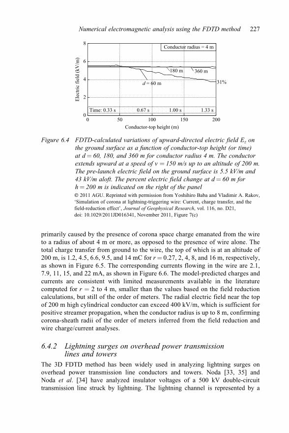
primarily caused by the presence of corona space charge emanated from the wireto a radius of about 4 m or more, as opposed to the presence of wire alone. Thetotal charge transfer from ground to the wire, the top of which is at an altitude of200 m, is 1.2, 4.5, 6.6, 9.5, and 14 mC for r ¼ 0.27, 2, 4, 8, and 16 m, respectively,as shown in Figure 6.5. The corresponding currents flowing in the wire are 2.1,7.9, 11, 15, and 22 mA, as shown in Figure 6.6. The model-predicted charges andcurrents are consistent with limited measurements available in the literaturecomputed for r ¼ 2 to 4 m, smaller than the values based on the field reductioncalculations, but still of the order of meters. The radial electric field near the topof 200 m high cylindrical conductor can exceed 400 kV/m, which is sufficient forpositive streamer propagation, when the conductor radius is up to 8 m, confirmingcorona-sheath radii of the order of meters inferred from the field reduction andwire charge/current analyses.

6.4.2 Lightning surges on overhead power transmissionlines and towers

The 3D FDTD method has been widely used in analyzing lightning surges onoverhead power transmission line conductors and towers. Noda [33, 35] andNoda et al. [34] have analyzed insulator voltages of a 500 kV double-circuittransmission line struck by lightning. The lightning channel is represented by a

0

2

4

6

8

0 50 100 150 200Conductor-top height (m)

Elec

tric

field

(kV

/m)

180 m

d = 60 m

0.67 s 1.00 s 1.33 sTime: 0.33 s

Conductor radius = 4 m

360 m

31%

Figure 6.4 FDTD-calculated variations of upward-directed electric field Ez onthe ground surface as a function of conductor-top height (or time)at d ¼ 60, 180, and 360 m for conductor radius 4 m. The conductorextends upward at a speed of v ¼ 150 m/s up to an altitude of 200 m.The pre-launch electric field on the ground surface is 5.5 kV/m and43 kV/m aloft. The percent electric field change at d ¼ 60 m forh ¼ 200 m is indicated on the right of the panel� 2011 AGU. Reprinted with permission from Yoshihiro Baba and Vladimir A. Rakov,‘Simulation of corona at lightning-triggering wire: Current, charge transfer, and thefield-reduction effect’, Journal of Geophysical Research, vol. 116, no. D21,doi: 10.1029/2011JD016341, November 2011, Figure 7(c)


0

5

10

15

20


Cha

rge

(mC

)Conductor radius = 16 m

4 m8 m

2 m0.27 m

Approximation byquadratic function

0.67 s 1.00 s 1.33 sTime: 0.33 s

Figure 6.5 FDTD-calculated variations of total charge on the surface of anupward-extending conductor (representing both the triggering wireand its corona sheath) as a function of conductor-top height (or time)for different conductor radii, 0.27, 2, 4, 8, and 16 m. The apparentirregularities (superimposed oscillations) are related to the presence ofconducting tubes simulating the effect of corona-space-charge layer atground. Broken-line curves are approximations by quadratic functionsused for evaluating corresponding currents shown in Figure 6.6� 2011 AGU. Reprinted with permission from Yoshihiro Baba and Vladimir A. Rakov,‘Simulation of corona at lightning-triggering wire: Current, charge transfer, and thefield-reduction effect’, Journal of Geophysical Research, vol. 116, no. D21,doi: 10.1029/2011JD016341, November 2011, Figure 8

0

10

20

30

40

Cur

rent

(mA

)

Conductor radius = 16 m

4 m8 m

0.27 m 2 m

0.67 s 1.00 s 1.33 sTime: 0.33 s


Figure 6.6 Currents flowing in the upward-extending conductor as a function ofconductor-top height (or time) for different conductor radii, 0.27, 2, 4,8, and 16 m, estimated as time derivatives of quadratic-function-approximated variations of charge shown in Figure 6.5� 2011 AGU. Reprinted with permission from Yoshihiro Baba and Vladimir A. Rakov,‘Simulation of corona at lightning-triggering wire: Current, charge transfer, and thefield-reduction effect’, Journal of Geophysical Research, vol. 116, no. D21,doi: 10.1029/2011JD016341, November 2011, Figure 9


vertical wire loaded by additional distributed series inductance [33, 34]. Yao et al.[40] have analyzed lightning currents in a 500-kV single-circuit tower struck bylightning and transient magnetic fields around the tower, with lightning representedby a lumped current source. Takami et al. [41] have studied lightning surges pro-pagating on inclined ground wires and phase conductors from a double-circuittower struck by lightning to the substation, and have shown that the surge voltagescomputed for realistic inclined power line conductors are significantly differentfrom those computed for horizontal conductors.

Baba and Rakov [32] have analyzed, using the 3D FDTD method, the char-acteristics of current wave propagating along perfectly conducting conical struc-tures (see Figure 6.7). A conical conductor is excited at its apex by a lumpedcurrent source in Figure 6.7(a), and it is excited at its base in Figure 6.7(b). They

8 cm

40 cm

ConeAir: e0, m0

1 m

Ez(q = p/4)Current source

Perfectly conducting planesEz(q = p/2)

Eh(q = p/4)

(a)

40 cmCone

Air: e0, m0

1 m

Ez(q = p/4)Current source

Perfectly conducting planes

Ez(q = p/2)

Eh(q = p/4)

8 cm

(b)

Figure 6.7 (a) A perfectly conducting cone in air excited at its apex by a currentsource having a height of 1 cm and a cross-sectional area of 1.5 cm �1.5 cm, and (b) a similar cone excited at its base by a current sourcehaving a height of 1 cm and an approximately circular cross-sectionalarea with a radius of 8.5 cm, analyzed using the FDTD method. Thecurrent source produces a Gaussian pulse having an amplitude of 1 Aand a half-peak width of 0.33 ns. The working volume of 2 m � 2 m �0.4 m, which is divided into 0.5 cm � 0.5 cm � 1 cm cells, issurrounded by six perfectly conducting planes� 2005 IEEE. Reprinted with permission from Yoshihiro Baba and Vladimir A. Rakov,‘On the interpretation of ground reflections observed in small-scale experiments:Simulating lightning strikes to towers’, IEEE Transactions on ElectromagneticCompatibility, vol. 47, no. 3, pp. 533–542, August 2005, Figure 1


have found that a current wave suffers no attenuation when it propagates downwardfrom the apex of the conical conductor to its base, but it attenuates significantlywhen it propagates upward from the base of the conical conductor to its apex, asseen in Figure 6.8. The current reflection coefficient at the base of the conicalconductor is close to 1, so that the equivalent grounding impedance of the con-ducting plane is close to zero. Our analysis suggests that the relatively highgrounding impedance (60 W) of conducting plane inferred from the small-scaleexperiments [89] is an engineering approximation to the neglected attenuation ofupward propagating waves. When the dependence of cone’s waveguiding prop-erties on the direction of propagation is taken into account, the results of

–0.5

0.0

0.5

1.0

1.5

0.0 0.5 1.0 1.5 2.0Time (ns)

Cur

rent

(A)

0 cm 5 cm 10 cm 20 cm

Cone excited at apex

Distance from cone apex

(a)

–0.5

0.0

0.5

1.0

1.5

0.0 0.5 1.0 1.5 2.0Time (ns)

Cur

rent

(A)

0 cm

Cone excited at base

Distance from cone base

10 cm20 cm

5 cm

(b)

Figure 6.8 Current waveforms for the conical conductor (see Figure 6.7) excitedat its (a) apex and (b) base at different vertical distances from thecurrent source, calculated using the FDTD method. The current pulsepropagates from the apex to the base (without attenuation) in (a) andfrom the base to the apex (with attenuation) in (b)� 2005 IEEE. Reprinted with permission from Yoshihiro Baba and Vladimir A. Rakov,‘On the interpretation of ground reflections observed in small-scale experiments:Simulating lightning strikes to towers’, IEEE Transactions on ElectromagneticCompatibility, vol. 47, no. 3, pp. 533–542, August 2005, Figure 2


small-scale experiments simulating lightning strikes to towers can be interpretedwithout invoking the fictitious grounding impedance of conducting plane.Representation of a vertical strike object by a uniform transmission line termi-nated in a fictitious high grounding impedance (60 W or so) appears to be justifiedin computing lightning-generated magnetic fields and relatively distant electricfields, but may be inadequate for calculating electric fields in the immediatevicinity of the object.

Baba and Rakov [31] have also shown that a current wave suffers attenuationas it propagates along a vertical perfect conductor of uniform, nonzero thickness(e.g., cylinder) above perfectly conducting ground excited at its bottom by a lumpedsource. The associated electromagnetic field structure is non-TEM, particularly nearthe source region. They decompose the ‘‘total’’ current in the conductor into twocomponents that they refer to as the ‘‘incident’’ and ‘‘scattered’’ currents. The‘‘incident’’ current serves as a reference (no attenuation) and is specified disregardingthe interaction of resultant electric and magnetic fields with the conductor, whilethe ‘‘scattered’’ current, found here using the 3D FDTD method, can be viewed as acorrection to account for that interaction. The scattered current modifies the inci-dent current, so that the resultant total current pulse appears attenuated. Theattenuation of the total current pulse is accompanied by the lengthening of its tail,such that the total charge transfer is independent of height. Takami et al. [36] haveshown experimentally that a current wave suffers attenuation and distortion when itpropagates along a vertical uniform conductor, both well reproduced by their 3DFDTD simulation.

Thang et al. [38] have analyzed, using the 3D FDTD method, lightning surgespropagating along overhead wires with corona discharge, and compared FDTD-computed results with the experiments of Inoue [90] and Wagner et al. [91]. InInoue’s experiment, a 12.65 mm radius, 1.4 km long overhead wire was employed.The radial progression of corona streamers from the wire is represented as theradial expansion of cylindrical conducting region, the conductivity of which is40 mS/m, as shown in Figure 6.9 [37]. The critical electric field on the surface ofthe 12.65 mm radius wire for corona initiation is set to E0 ¼ 2.4 MV/m. The cri-tical background electric field for streamer propagation is set to Ecp ¼ 0.5 MV/mfor positive voltage application and Ecn ¼ 1.5 MV/m for negative voltageapplication. Figure 6.10 shows the FDTD-computed waveforms (note wavefrontdistortion and attenuation at later times) of surge voltages at three different dis-tances from the energized end of the wire, which agree reasonably well with thecorresponding measured waveforms. Also, the FDTD-computed waveforms ofsurge voltages induced on a nearby parallel bundled conductor agree fairly wellwith the corresponding measured waveforms, although they are not shown here. Inthe FDTD simulation, the conductor system is accommodated in a working volumeof 60 m � 1460 m � 80 m, which is divided nonuniformly into rectangular cells.The side length in y direction (conductor-axis direction) of all the cells is 1 m(constant). Cell sides along x and z axes are not constant: 5.5 cm in the vicinity(220 cm � 220 cm) of the wire, increasing gradually (to 10, 20, and 100 cm)beyond that region.


Thang et al. [39] have analyzed, using the 3D FDTD method, transient voltagesacross insulators of a 60 m high transmission line whose overhead ground wire isstruck by lightning. The progression of corona streamers from the ground wireis represented as the radial expansion of cylindrical conducting region aroundthe wire. The lightning channel is represented by a vertical phased-current-sourcearray, along which a current wave propagates upward at speed 130 m/ms. On thebasis of the computed results, the role of corona discharge at the ground wire ontransient insulator voltages is examined. The insulator voltages are reduced bycorona discharge on the ground wire. The reduction of insulator-voltage peak dueto the ground-wire corona is not very significant: the upper-, middle-, and lower-phase-voltage peaks are reduced by 15%, 14%, and 13% for a positive-strokewith 50 kA peak and 3 ms risetime current, and those for negative stroke withthe same current waveform parameters are reduced by 10%, 9%, and 8%,respectively. In the FDTD simulation, the conductor system is accommodated in aworking volume of 400 m � 500 m � 750 m, which is divided nonuniformly intorectangular cells: 9 cm in the vicinity of the ground wire and each of the phaseconductors, increasing gradually (to 50, 100, and 500 cm) beyond that region.

x

z

y

Time step: n n + 1

Ezbn > 0.46E0

Wire

scor = 40 μS/m

(a)

x

z

y

Time step: n n + 1

rcn+1

Ezbn

Ezan

Exln Exr

n

from Ec and qn

(b)

scor = 40 μS/m

Figure 6.9 FDTD representations of (a) inception of corona discharge at the wiresurface and (b) radial expansion of corona discharge� 2012 IEEE. Reprinted with permission from Tran Huu Thang, Yoshihiro Baba, NaotoNagaoka; Akihiro Ametani, Jun Takami, Shigemitsu Okabe, and Vladimir A. Rakov,‘A simplified model of corona discharge on overhead wire for FDTD computations’,IEEE Transactions on Electromagnetic Compatibility, vol. 54, no. 3, pp. 585–593,June 2012, Figure 3


6.4.3 Lightning surges on overhead power distribution linesBaba and Rakov [42] have analyzed, using the 3D FDTD method, transient vol-tages on an overhead single wire above lossy ground due to nearby lightning strikesto flat ground and to a 100 m high object. The nearby lightning channel with orwithout the strike object is represented by a vertical phased-current-source array.The conductor system is accommodated in a working volume of 1,400 m �600 m � 850 m, which is divided uniformly into cubic cells of 5 m � 5 m � 5 m.They have examined the ratios of magnitudes of lightning-induced voltages for thecases of strikes to a 100 m high object and to flat ground as a function of distancefrom the lightning channel, d, current reflection coefficients at the top of the strikeobject, rtop, and at the bottom of the strike object, rbot, the current reflectioncoefficient at the channel base (in the case of strikes to flat ground), rgr, and thereturn-stroke speed, v. The ratio of magnitudes of lightning-induced voltages fortall-object and flat-ground cases increases with increasing d, decreasing rbot (<1),decreasing rtop (<0, except for the case of rbot ¼ 0), and decreasing v (<c). Theratio is larger than unity (strike object serves to enhance the induced voltage) ford ¼ 40 to 200 m and realistic conditions such as rbot ¼ (rgr) ¼ 1, rtop ¼�0.5,and v ¼ c/3, but becomes smaller than unity (lightning-induced voltage for the

00

500

+1580 kV

1,000

1,500

Computed

Measured by Inoue

1,050 m

Time (μs)

700 md = 350 m

Applied (measured at d = 0)

2,000

Vol

tage

(kV

)

1 2 3

Figure 6.10 FDTD-computed (for scor ¼ 40 mS/m and E0 ¼ 2.4 MV/m) andmeasured waveforms of surge voltage at d¼ 0, 350, 700, and 1,050 mfrom the energized end of the 12.65 mm radius, 1.4 km longhorizontal wire located 22.2 m above ground of conductivity10 mS/m. The applied voltage is positive and Ecp ¼ 0.5 MV/m.Applied voltage peak is 1,580 kV� 2012 IEEE. Reprinted with permission from Tran Huu Thang, Yoshihiro Baba,Naoto Nagaoka, Akihiro Ametani, Jun Takami, Shigemitsu Okabe, and Vladimir A.Rakov, ‘FDTD simulation of lightning surges on overhead wires in the presence ofcorona discharge’, IEEE Transactions on Electromagnetic Compatibility, vol. 54,no. 6, pp. 1234–1243, December 2012, Figure 2(a)


tall-object case is smaller than for the flat-ground case) under some special con-ditions such as rbot ¼ (rgr) ¼ 1, rtop ¼ 0, and v ¼ c.

Sumitani et al. [47] have computed lightning-induced voltages on an overheadtwo-wire line using the 3D FDTD method in which spatial discretization is fine inthe vicinity of overhead wires and coarse in the rest of the computational domain.They used the so-called subgridding method, which is different from nonuniformgridding and more efficient.

Tatematsu and Noda [45, 49] have analyzed lightning-induced voltages on anoverhead three-phase distribution line with an overhead ground wire and lightningarresters above perfectly conducting and lossy ground using the 3D FDTD method.The nonlinear voltage–current (V–I) relation of the arrester is represented by piece-wise linear curves, which is based on the measured V–I curve. The nearby lightningchannel is represented by a vertical phased-current-source array. The conductorsystem is accommodated in a working volume of 1,400 m � 650 m � 700 m, whichis divided nonuniformly into rectangular cells: 2 cm in the vicinity of the horizontalground wires, increasing gradually (to 200 cm) beyond that region.

Thang et al. [48] have computed, using the 3D FDTD method, lightning-inducedvoltages at different points along a 5 mm radius, 1 km long single overhead wireshown in Figure 6.11. Corona space charge around the wire is considered. FDTDcomputations are performed using a 3D nonuniform grid. The progression of coronastreamers from the wire is represented as the radial expansion of cylindrical weaklyconducting (40 mS/m) region around the wire. The magnitudes of FDTD-computedlightning-induced voltages in the presence of corona discharge are larger than thosecomputed without considering corona, as shown in Figure 6.12. The observedtrend, although less pronounced, is in agreement with that reported by Nucci et al.[92]. When corona is considered, there is a tendency for induced-voltage risetimesto increase. Figure 6.13 shows the variation with time of corona radius at differentpoints along the wire and the variation of corona radius along the wire at time 5 ms,computed for the case of perfectly conducting ground. The maximum radius ofcorona region around the wire for stroke location A (see Figure 6.11) and 35 kAcurrent peak is 19.8 cm. It follows from Figure 6.13 that the presence of lightning-induced corona on the wire makes the transmission line (formed by the wire and itsimage) nonuniform. Note that corona-radius variation is step-like due to the size ofrectangular cells employed in the FDTD computations. It appears that the dis-tributed impedance discontinuity, associated with corona development on the wire,is the primary reason for higher induced-voltage peaks and longer voltage risetimescompared to the case without corona.

Ren et al. [43], using the 2D cylindrical FDTD method instead of approximateexpressions, evaluated the electric fields over lossy ground, and calculated thelightning-induced voltages on an overhead two-wire distribution line using theFDTD-computed fields with Agrawal et al.’s field-to-wire coupling model [93].One of the reasons for using the two-step or hybrid approach is apparently relatedto a difficulty of representing closely spaced overhead thin wires in the 3D uniform-grid FDTD method. Zhang et al. [50] have used the same approach for investi-gating the influence of horizontally stratified ground on lightning-induced voltages.


Yang et al. [46] have employed a different two-step approach for evaluatinglightning-induced voltages on an overhead single wire above lossy ground. Thefirst step is a 2D cylindrical FDTD computation of electric and magnetic fieldsgenerated by a nearby lightning strike that illuminate the 3D volume accom-modating the overhead wire. The second step is a 3D FDTD computation oflightning-induced voltages on the overhead wire illuminated by incident electro-magnetic fields from the boundary of the 3D working volume.

Matsuura et al. [44] have analyzed transient voltages due to direct lightningstrikes to the overhead ground wire of three-phase distribution line over lossyground using the 3D FDTD method. The working volume is divided nonuniformly.The lightning channel attached to the ground wire is represented by a verticalperfectly conducting wire, excited by a lumped current source inserted between thesimulated lightning channel and the ground wire.

Phased current sourcearray representinglightning channel

Ground

1.200 m

400 m 1.200 m

500 m

50 m

100 m

100 m

50 m

50 m

500 m 500 m

(A) (B)

(A)

(B)

50 m

600 m

100 m

y

z x

z

x y

7.5 m

(a) (b)

Figure 6.11 (a) Plan (xy plane) and (b) side (yz plane) views of a 5 mm radius,1 km long overhead horizontal wire located 7.5 m above ground.Corona discharge is assumed to occur only on the horizontal wire.Ground strike points are shown in (a), and simulated lightingchannels are shown in (b)� 2014 IEEE. Reprinted with permission from Tran Huu Thang, Yoshihiro Baba,Naoto Nagaoka, Akihiro Ametani, Naoki Itamoto, and Vladimir A. Rakov, ‘FDTDsimulations of corona effect on lightning-induced voltages’, IEEE Transactions onElectromagnetic Compatibility, vol. 56, no. 1, pp. 168–176, February 2014, Figure 1


6.4.4 Lightning electromagnetic environment in power substationOliveira and Sobrinho [51], using the 3D FDTD method, have analyzed electro-magnetic environment in an air-insulated power substation struck by lightning.Electric potentials and step and touch voltages are calculated for a realistic con-figuration. The lightning channel is not considered, and the lightning current isappeared to be injected by a lumped current source.

6.4.5 Lightning electromagnetic environment in airborne vehiclesApra et al. [52], using the 3D FDTD method, have analyzed transient magneticfields and voltages induced on cables in an airborne vehicle struck by lightning.The lightning channel is represented by a vertical perfectly conducting wire.A lumped current source appears to be used as an exciter. The airborne vehicle,which is partially made of carbon fiber composite of conductivity 1.5 � 104 S/m, is22 m in length, 30 m in wing span, and 9 m in height. It is represented with cubiccells of 0.1 m � 0.1 m � 0.1 m. Perrin et al. [53] carried out a similar 3D FDTDcomputation for estimating currents induced on cables in an airborne vehicle struckby lightning. The representation of lightning channel is not given in [53]. Theairborne vehicle, which is partially made of carbon fiber composite of conductivity1,000 S/m, is represented with cubic cells of 5 cm � 5 cm � 5 cm.

00

50

100

Vol

tage

(kV

)

150

200

sgr = 0.01 S/m250

1 2 3

0 m

With coronaWithout corona

250 m

500 m

Time (μs)4 5

Figure 6.12 Negative stroke at location A (see Figure 6.11): FDTD-computed(for scor ¼ 40 mS/m, E0 ¼ 2.9 MV/m, and Ecn ¼ 1.5 MV/m)waveforms of induced voltages at d ¼ 0, 250, and 500 m fromeither end of the 5 mm radius, 1.0 km long horizontal wire. Thecomputations were performed for sgr ¼ 0.01 S/m� 2014 IEEE. Reprinted with permission from Tran Huu Thang, Yoshihiro Baba,Naoto Nagaoka, Akihiro Ametani, Naoki Itamoto, and Vladimir A. Rakov, ‘FDTDsimulations of corona effect on lightning-induced voltages’, IEEE Transactions onElectromagnetic Compatibility, vol. 56, no. 1, pp. 168–176, February 2014, Figure 4(b)


0

5000

5

10

Cor

ona

radi

us (c

m)

15

20

25

450 400 350 300 250 200Distance (m)

(b)

(a)

0

5

10

Cor

ona

radi

us (c

m)

15

20

25

1 2 3 4

250 m

300 m

350 m400 m

450 m

d = 500 msgr = ∞

5

Time (μs)

Figure 6.13 Negative stroke at location A: (a) Time variation of corona radiusat d ¼ 500, 450, 400, 350, 300, and 250 m from either end of the5 mm radius, 1.0 km long horizontal wire located above perfectlyconducting ground, and (b) corona radius as a function of distancefrom either end of the wire at time 5 ms� 2014 IEEE. Reprinted with permission from Tran Huu Thang, Yoshihiro Baba,Naoto Nagaoka, Akihiro Ametani, Naoki Itamoto, and Vladimir A. Rakov, ‘FDTDsimulations of corona effect on lightning-induced voltages’, IEEE Transactions onElectromagnetic Compatibility, vol. 56, no. 1, pp. 168–176, February 2014, Figure 6


6.4.6 Lightning surges and electromagnetic environmentin buildings

Nagaoka et al. [54] analyzed, using the 3D FDTD method, the transient distributionof current in a seismic-isolated 20 m high building struck by lightning and poten-tials at different parts of the building. The building is represented by a perfectlyconducting lattice structure of 8 m � 8 m � 20 m, and is represented with cubiccells of 1 m � 1 m � 1 m. Each pillar is connected to ground via a 1 or 2 mHinductor that represents a coiled wire bridging the seismic rubber insulator.The lightning channel is represented by a vertical perfectly conducting wire.A lumped current source is inserted between the lightning channel and the center ofthe building roof. Chen et al. [56] performed a similar 3D FDTD simulation, butthe building has no seismic wiring.

Ishii et al. [57] analyzed, using the 3D FDTD method, the transient distribu-tion of current in a 25 m high building struck by lightning and potentialsat different parts of the building. The building is represented by a perfectlyconducting lattice structure of 20 m � 20 m � 25 m, and is represented with cubiccells of 0.5 m � 0.5 m � 0.5 m. The lightning channel is represented by a vertical1 W/m resistive wire. An ideal current source in parallel with a 600 W resistor isinserted between the lightning channel and the 5 m long lightning rod on thebuilding roof. Surge protective devices for suppressing lightning overvoltages areincorporated in the simulation.

Chamie et al. [58] analyzed, using the 3D FDTD method, voltages induced onelectrical wirings of nine buildings of height 24 m, due to lightning strikes to thenearby 50 m high radio base station. Each building is represented by a perfectlyconducting lattice structure of 24 m � 12.8 m � 24 m with walls and floors of zeroconductivity and relative permittivity 7.5. It is represented with cubic cells of0.2 m � 0.2 m � 0.2 m. The lightning channel is represented by a vertical wireloaded by additional distributed series inductance. A lumped current source is usedas an exciter. Oshiro et al. [55] analyzed, using the 3D FDTD method, voltagesinduced on an electrical wiring in a house by nearby lightning strikes. The lightningchannel is represented by a vertical phased-current-source array.

6.4.7 Surges on grounding electrodesTanabe [13] has first applied the 3D FDTD method to analyzing the surge responseof a vertical grounding electrode of 0.5 m � 0.5 m � 3 m, and shown that FDTD-computed response agrees well with the corresponding measured one. Tsumuraet al. [60] analyzed the surge response of horizontal grounding electrode using the3D FDTD method, and used the FDTD-computed response to test the validity of asimplified equivalent circuit model of horizontal grounding electrode.

Baba et al. [59] have proposed a procedure for representing thin cylindricalwires buried in lossy ground, which is implemented in 3D FDTD surge simulations.Xiong et al. [62, 63] have proposed procedures for representing flat thin wiresburied in lossy ground, which is used in 3D FDTD surge simulations. Here ‘‘thin’’means the radius of the thickness of the conductor is smaller than the side length of


cell employed. Xiong et al. [64] have also carried out surge simulations for asymmetrical vertical grounding electrode using the 2D cylindrical FDTD method.

Ala et al. [61] considered the soil ionization around a grounding electrode intheir 3D FDTD computations. The ionization model is based on the dynamic soil-resistivity model of Liew and Darveniza [94]. In the model, the resistivity of eachsoil-representing cell is controlled by the instantaneous value of the electric fieldthere and time. Otani et al. [65] have applied the soil ionization model to analyzingdifferent grounding electrodes, and compared 3D FDTD-computed responses withcorresponding measured one.

6.5 Summary

In this chapter, the fundamental theory of the FDTD method has been reviewed,and advantages and disadvantages of the FDTD method in comparison with otherrepresentative NEA methods have been identified. Also, seven representations ofthe lightning return-stroke channel used to date have been described. Furthermore,the representative applications of the FDTD method have been reviewed. Theyinclude simulations of (i) lightning electromagnetic fields at close and far distances,(ii) lightning surges on overhead power transmission lines and towers, (iii) light-ning surges on overhead power distribution and telecommunication lines,(iv) lightning electromagnetic environment in power substations, (v) lightningelectromagnetic environment in airborne vehicles, (vi) lightning surges and elec-tromagnetic environment in buildings, and (vii) surges on grounding electrodes.

References

[1] Harrington R. F. Field Computation by Moment Methods, Macmillan,New York, 1968.

[2] Sadiku M. N. O. ‘A simple introduction to finite element analysis of elec-tromagnetic problems’. IEEE Transactions on Education. 1989, vol. 32,no. 2, pp. 85–93.

[3] A. Ruehli, ‘Equivalent circuit models for three-dimensional multiconductorsystems’. IEEE Transactions on Microwave Theory and Techniques. 1974,vol. 22, no. 3, pp. 216–221.

[4] Visacro S., Soares A. Jr. ‘HEM: A model for simulation of lightning relatedengineering problems’. IEEE Transactions on Power Delivery. 2005,vol. 20, no. 2, pp. 1206–1207.

[5] Johns P. B., Beurle R. B. ‘Numerical solutions of 2-dimensional scatteringproblems using a transmission-line matrix’. Proceedings of the IEE. 1971,vol. 118, no. 9, pp. 1203–1208.

[6] Yee K. S. ‘Numerical solution of initial boundary value problems involvingMaxwell’s equations in isotropic media’. IEEE Transactions on Antennasand Propagation. 1966, vol. 14, no. 3, pp. 302–307.


[7] Baba Y., Rakov V. A. ‘Electromagnetic models of the lightning returnstroke’. Journal of Geophysical Research. 2007, vol. 112, no. D4,doi:10.1029/2006JD007222, 17 pp.

[8] Baba Y., Rakov V. A. ‘Applications of electromagnetic models of thelightning return stroke’. IEEE Transactions on Power Delivery. 2008,vol. 23, no. 2, pp. 800–811.

[9] Baba Y., Rakov V. A. ‘Electric and magnetic fields predicted by differentelectromagnetic models of the lightning return stroke versus measuredfields’. IEEE Transactions on Electromagnetic Compatibility. 2009, vol. 51,no. 3, pp. 479–483.

[10] Baba Y., Rakov V. A. ‘Electromagnetic models of lightning return strokes’.In Lightning Electromagnetics (V. Cooray, Ed.). IET. 2012, London, UK.pp. 263–313.

[11] CIGRE Working Group C4.501. Guide for Numerical ElectromagneticAnalysis Methods: Application to Surge Phenomena and Comparison withCircuit Theory-based Approach. Technical Brochure. 2013, no. 543, ISBN:978-2-85873-237-1.

[12] Baba Y., Rakov V. A. ‘On the transmission line model for lightning returnstroke representation’. Geophysical Research Letters. 2013, vol. 30, no. 24,4 pp.

[13] Tanabe K. ‘Novel method for analyzing dynamic behavior of groundingsystems based on the finite-difference time-domain method’. IEEE PowerEngineering Review. 2001, vol. 21, no. 9, pp. 55–57.

[14] Yang C., Zhou B. ‘Calculation methods of electromagnetic fields very closeto lightning’. IEEE Transactions on Electromagnetic Compatibility. 2004,vol. 46, no. 1, pp. 133–141.

[15] Berenger J.-P. ‘Long range propagation of lightning pulses using the FDTDmethod’. IEEE Transactions on Electromagnetic Compatibility. 2005,vol. 47, no. 4, pp. 1008–1011.

[16] Hu W., Cummer S. A. ‘An FDTD model for low and high altitude lightning-generated EM fields’. IEEE Transactions on Antennas and Propagation.2006, vol. 54, no. 5, pp. 1513–1522.

[17] Baba Y., Rakov V. A. ‘Electromagnetic fields at the top of a tall buildingassociated with nearby lightning return strokes’. IEEE Transactions onElectromagnetic Compatibility. 2007, vol. 49, no. 3, pp. 632–643.

[18] Baba Y., Rakov V. A. ‘Influence of strike object grounding on close light-ning electric fields’. Journal of Geophysical Research. 2008, vol. 113,no. D12, doi:10.1029/2008JD009811, 18 pp.

[19] Mimouni A., Rachidi F., Azzouz Z. ‘A finite-difference time-domainapproach for the evaluation of electromagnetic fields radiated by lightningstrikes to tall structures’. Journal of Electrostatics. 2008, vol. 66, no. 9,pp. 504–513.

[20] Shoory A., Mimouni A., Rachidi F., Cooray V., Moini R., Sadeghi S. H. H.‘Validity of simplified approaches for the evaluation of lightning electro-magnetic fields above a horizontally stratified ground’. IEEE Transactionson Electromagnetic Compatibility. 2010, vol. 52, no. 3, pp. 657–663.


[21] Oikawa T., Sonoda J., Sato M., Honma N., Ikegawa Y. ‘Analysis of lightningelectromagnetic field on large-scale terrain model using three-dimensionalMW-FDTD parallel computation’ (in Japanese). IEEJ Transactions on Fun-damentals and Materials. 2012, vol. 132, no. 1, pp. 44–50.

[22] Haddad M., Rakov V. A., Cummer S. ‘New measurements of lightningelectric fields in Florida: Waveform characteristics, interaction with theionosphere, and peak current estimates’. Journal of Geophysical Research.2012, vol. 117, no. D10, doi:10.1029/2011JD017196, 26 pp.

[23 ] Zhang Q., Li D., Fan Y., Zhang Y., Gao J. ‘Examination of the Cooray-Rubinstein (C-R) formula for a mixed propagation path by using FDTD’.Journal of Geophysical Research. 2012, vol. 117, no. D15, doi:10.1029/2011JD017331, 7 pp.

[24] Khosravi-Farsani M., Moini R., Sadeghi S. H. H., Rachidi F. ‘On the validityof approximate formulas for the evaluation of the lightning electromagneticfields in the presence of a lossy ground’. IEEE Transactions on Electro-magnetic Compatibility. 2013, vol. 55, no. 2, pp. 362–370.

[25] Zhang S., Wu Q. ‘A new perspective to the attributes of lightning electro-magnetic field above the ground’. Journal of Electrostatics. 2013, vol. 71,no. 4, pp. 703–711.

[26] Li D., Zhang Q., Liu T., Wang Z. ‘Validation of the Cooray-Rubinstein(C-R) formula for a rough ground surface by using three-dimensional(3-D) FDTD’. Journal of Geophysical Research. 2013, vol. 118, no. 22,doi:10.1002/2013JD020078, 6 pp.

[27] Zhang Q., Tang V., Gao J., Zhang L., Li D. ‘The influence of the horizon-tally stratified conducting ground on the lightning-induced voltages’.IEEE Transactions on Electromagnetic Compatibility. 2014, vol. 56, no. 1,pp. 143–148.

[28] Li D., Zhang Q., Wang Z., Liu T. ‘Computation of lightning horizontal fieldover the two-dimensional rough ground by using the three-dimensionalFDTD’. IEEE Transactions on Electromagnetic Compatibility. 2014, vol. 56,no. 1, pp. 143–148.

[29] Mimouni A., Rachidi F., Rubinstein M. ‘Electromagnetic fields of a light-ning return stroke in presence of a stratified ground’. IEEE Transactions onElectromagnetic Compatibility. 2014, vol. 56, no. 2, pp. 413–418.

[30] Baba Y., Rakov V. A. ‘Simulation of corona at lightning-triggeringwire: Current, charge transfer, and the field-reduction effect’. Journal ofGeophysical Research. 2011, vol. 116, no. D21, doi:10.1029/2011JD016341,12 pp.

[31] Baba Y., Rakov V. A. ‘On the mechanism of attenuation of current wavespropagating along a vertical perfectly conducting wire above ground:Application to lightning’. IEEE Transactions on Electromagnetic Compat-ibility. 2005, vol. 47, no. 3, pp. 521–532.

[32] Baba Y., Rakov V. A. ‘On the interpretation of ground reflections observedin small-scale experiments: Simulating lightning strikes to towers’. IEEETransactions on Electromagnetic Compatibility. 2005, vol. 47, no. 3,pp. 533–542.


[33] Noda T. ‘A tower model for lightning overvoltage studies based on the resultof an FDTD simulation’ (in Japanese). IEEJ Transactions on Power andEnergy. 2007, vol. 127, no. 2, pp. 379–388.

[34] Noda T., Tatematsu A., Yokoyama S. ‘Improvements of an FDTD-basedsurge simulation code and its application to the lightning overvoltage cal-culation of a transmission tower’. Electric Power Systems Research. 2007,vol. 77, no. 11, pp. 1495–1500.

[35] Noda T. ‘A numerical simulation of transient electromagnetic fields forobtaining the step response of a transmission tower using the FDTDmethod’. IEEE Transactions on Power Delivery. 2008, vol. 23, no. 2,pp. 1262–1263.

[36] Takami J., Tsuboi T., Okabe S. ‘Measured distortion of current wavesand electrical potentials with propagation of a spherical wave in anelectromagnetic field’. IEEE Transactions on Electromagnetic Compat-ibility. 2010, vol. 52, no. 3, pp. 753–756.

[37] Thang T. H., Baba Y., Nagaoka N., Ametani A., Takami J., Okabe S., RakovV. A. ‘A simplified model of corona discharge on overhead wire for FDTDcomputations’. IEEE Transactions on Electromagnetic Compatibility. 2012,vol. 54, no. 3, pp. 585–593.

[38] Thang T. H., Baba Y., Nagaoka N., Ametani A., Takami J., Okabe S.,Rakov V. A. ‘FDTD simulation of lightning surges on overhead wires in thepresence of corona discharge’. IEEE Transactions on ElectromagneticCompatibility. 2012, vol. 54, no. 6, pp. 1234–1243.

[39] Thang T. H., Baba Y., Nagaoka N., Ametani A., Itamoto N., Rakov V. A.‘FDTD simulation of insulator voltages at a lightning-struck tower con-sidering ground-wire corona’. IEEE Transactions on Power Delivery. 2013,vol. 28, no. 3, pp. 1635–1642.

[40] Yao C., Wu H., Mi Y., Ma Y., Shen Y., Wang L. ‘Finite difference timedomain simulation of lightning transient electromagnetic fields on trans-mission lines’. IEEE Transactions on Dielectrics and Electrical Insulation.2013, vol. 20, no. 4, pp. 1239–1246.

[41] Takami J., Tsuboi T., Yamamoto K., Okabe S., Baba Y., Ametani A.‘Lightning surge response of a double-circuit transmission tower withincoming lines to a substation through FDTD simulation’. IEEE Transac-tions on Dielectrics and Insulation. 2014, vol. 21, no. 1, pp. 96–104.

[42] Baba Y., Rakov V. A. ‘Voltages induced on an overhead wire by lightningstrikes to a nearby tall grounded object’. IEEE Transactions on Electro-magnetic Compatibility. 2006, vol. 48, no. 1, pp. 212–224.

[43] Ren H.-M., Zhou B.-H., Rakov V. A., Shi L.-H., Gao C., Yang J.-H. ‘Ana-lysis of lightning-induced voltages on overhead lines using a 2-D FDTDmethod and Agrawal coupling model’. IEEE Transactions on Electro-magnetic Compatibility. 2008, vol. 50, no. 3, pp. 651–659.

[44] Matsuura S., Tatematsu A., Noda T., Yokoyama S. ‘A simulation study oflightning surge characteristics of a distribution line using the FDTDmethod’. IEEJ Transactions on Power and Energy. 2009, vol. 129, no. 10,pp. 1225–1232.


[45] Tatematsu A., Noda T. ‘Development of a technique for representing light-ning arresters in the surge simulations based on the FDTD method and itsapplication to the calculation of lightning-induced voltages on a distributionline’ (in Japanese). IEEJ Transactions on Power and Energy. 2010, vol. 130,no. 3, pp. 373–382.

[46] Yang B., Zhou B.-H., Gao C., Shi L.-H., Chen B., Chen H.-L. ‘Using a two-step finite-difference time-domain method to analyze lightning-inducedvoltages on transmission lines’. IEEE Transactions on ElectromagneticCompatibility. 2011, vol. 53, no. 1, pp. 256–260.

[47] Sumitani H., Takeshima T., Baba Y., Nagaoka N., Ametani A., Takami J.,Okabe S., Rakov V. A. ‘3-D FDTD computation of lightning-induced vol-tages on an overhead two-wire distribution line’. IEEE Transactions onElectromagnetic Compatibility. 2012, vol. 54, no. 5, pp. 1161–1168.

[48] Thang T. H., Baba Y., Nagaoka N., Ametani A., Itamoto N., Rakov V. A.‘FDTD simulations of corona effect on lightning-induced voltages’. IEEETransactions on Electromagnetic Compatibility. 2014, vol. 56, no. 1,pp. 168–176.

[49] Tatematsu A., Noda T. ‘Three-dimensional FDTD calculation of lightning-induced voltages on a multiphase distribution line with the lightning arrest-ers and an overhead shielding wire’. IEEE Transactions on ElectromagneticCompatibility. 2014, vol. 56, no. 1, pp. 159–167.

[50] Zhang Q., Tang V., Gao J., Zhang L., Li D. ‘The Influence of the horizon-tally stratified conducting ground on the lightning-.induced voltages’.IEEE Transactions on Electromagnetic Compatibility. 2014, vol. 56, no. 2,pp. 435–443.

[51] Oliveira R. Melo e Silva de, Sobrinho C. L. da Silva Souza. ‘Computationalenvironment for simulating lightning strokes in a power substation by finite-difference time-domain method’. IEEE Transactions on ElectromagneticCompatibility. 2009, vol. 51, no. 4, pp. 995–1000.

[52] Apra M., D’Amore M., Gigliotti K., Sarto M. S., Volpi V. ‘Lightningindirect effects certification of a transport aircraft by numerical simulation’.IEEE Transactions on Electromagnetic Compatibility. 2008, vol. 50, no. 3,pp. 513–523.

[53] Perrin E., Guiffaut C., Reineix A., Tristant F. ‘Using a design-of-experimenttechnique to consider the wire harness load impedances in the FDTD modelof an aircraft struck by lightning’. IEEE Transactions on ElectromagneticCompatibility. 2013, vol. 55, no. 4, pp. 747–753.

[54] Nagaoka N., Morita H., Baba Y., Ametani A. ‘Numerical simulations oflightning surge responses in a seismic isolated building by FDTD andEMTP’. IEEJ Transactions on Power and Energy. 2008, vol. 128, no. 2,pp. 473–478.

[55] Oshiro R., Isa S., Kaneko E. ‘A simulation study of induced surge on lowvoltage distribution system nearby the lightning point’ (in Japanese). IEEJTransactions on Power and Energy. 2010, vol. 130, no. 7, pp. 687–693.

[56] Chen J., Zhou B., Zhao F., Qiu S. ‘Finite-difference time-domain analysis ofthe electromagnetic environment in a reinforced concrete structure when


struck by lightning’. IEEE Transactions on Electromagnetic Compatibility.2010, vol. 52, no. 4, pp. 914–920.

[57] Ishii M., Miyabe K., Tatematsu A. ‘Induced voltages and currents on elec-trical wirings in building directly hit by lightning’. Electric Power SystemsResearch. 2012, vol. 85, pp. 2–6.

[58] Filho Ricardo H.T. Chamie, Carvalho Lorena F.P., Machado Pericles L.,Oliveira Rodrigo M.S. de. ‘Analysis of voltages induced on power outletsdue to atmospheric discharges on radio base stations’. Applied MathematicalModelling. 2013, vol. 37, no. 9, pp. 6530–6542.

[59] Baba Y., Nagaoka N., Ametani A. ‘Modeling of thin wires in a lossymedium for FDTD simulations’. IEEE Transactions on ElectromagneticCompatibility. 2005, vol. 47, no. 1, pp. 54–60.

[60] Tsumura M., Baba Y., Nagaoka N., Ametani A. ‘FDTD simulation of ahorizontal grounding electrode and modeling of its equivalent circuit’. IEEETransactions on Electromagnetic Compatibility. 2006, vol. 48, no. 4,pp. 817–825.

[61] Ala G., Buccheri P. L., Romano P., Viola F. ‘Finite difference time domainsimulation of earth electrodes soil ionisation under lightning surge condition’.IET Science, Measurement & Technology. 2008, vol. 2, no. 3, pp. 134–145.

[62] Xiong R., Chen B., Mao Y.-F., Deng W., Wu Q., Qiu Y.-Y. ‘FDTD mod-eling of the earthing conductor in the transient grounding resistance analy-sis’. IEEE Trans. Antennas and Wireless Propagation Letters. 2012, vol. 11,pp. 957–960.

[63] Xiong R., Chen B., Fang D. ‘An algorithm for the FDTD modeling of flatelectrodes in grounding systems’. IEEE Transactions on Antennas andPropagation. 2014, vol. 62, no. 1, pp. 345–353.

[64] Xiong R., Chen B., Zhou B. H., Gao C. ‘Optimized programs for shapedconductive backfill material of grounding systems based on the FDTDsimulations’. IEEE Transactions on Power Delivery. 2014, vol. 29, no. 4,pp. 1744–1751.

[65] Otani K., Shiraki Y., Baba Y., Nagaoka N., Ametani A., Itamoto N. ‘FDTDsurge analysis of grounding electrodes considering soil ionization’. ElectricPower Systems Research. 2014, vol. 113, pp. 171–179.

[66] Liao Z. P., Wong H. L., Yang B. P., Yuan Y. F. ‘A transmission boundaryfor transient wave analysis’. Science Sinica. 1984, vol. A27, no. 10,pp. 1063–1076.

[67] Berenger J. P. ‘A perfectly matched layer for the absorption of electro-magnetic waves’. Journal of Computational Physics. 1994, vol. 114,pp. 185–200.

[68] Rakov V. A., Dulzon A. A. ‘Calculated electromagnetic fields of lightningreturn stroke’ (in Russian). Tekh. Elektrodinam. 1987, vol. 1, pp. 87–89.

[69] Rakov V. A. ‘Lightning return stroke speed’. Journal of Lightning Research.2007, vol. 1, pp. 80–89.

[70] Gorin B. N., Shkilev A. V. ‘Measurements of lightning currents at theOstankino tower’ (in Russian). Electrichestrvo. 1984, vol. 8, pp. 64, 65.


[71] Podgorski A. S., Landt J. A. ‘Three dimensional time domain modelling oflightning’. IEEE Trans. Power Delivery. 1987, vol. 2, no. 3, pp. 931–938.

[72] Kato S., Narita T., Yamada T., Zaima E. ‘Simulation of electromagneticfield in lightning to tall tower’. Paper presented at 11th International Sym-posium on High Voltage Engineering, no. 467, London, UK, August 1999.

[73] Rakov V. A. ‘Some inferences on the propagation mechanisms of dart lea-ders and return strokes’. Journal of Geophysical Research. 1998, vol. 103,no. D2, pp. 1879–1887.

[74] Bonyadi-ram S., Moini R., Sadeghi S. H. H., Rakov V. A. ‘On representationof lightning return stroke as a lossy monopole antenna with inductive load-ing’. IEEE Transactions on Electromagnetic Compatibility. 2008, vol. 50,no. 1, pp. 118–127.

[75] Idone V. P., Orville R. E. ‘Lightning return stroke velocities in the Thun-derstorm Research International Program (TRIP)’. Journal of GeophysicalResearch. 1982, vol. 87, pp. 4903–4915.

[76] Moini R., Kordi B., Rafi G. Z., Rakov V. A. ‘A new lightning return strokemodel based on antenna theory’. Journal of Geophysical Research. 2000,vol. 105, no. D24, pp. 29693–29702.

[77] Kato S., Takinami T., Hirai T., Okabe S. ‘A study of lightning channelmodel in numerical electromagnetic field computation’ (in Japanese). Paperpresented at 2001 IEEJ National Convention, no. 7-140, Nagoya, Japan,March 2001.

[78] Miyazaki S., Ishii M. ‘Reproduction of electromagnetic fields associatedwith lightning return stroke to a high structure using FDTD method’(in Japanese). Paper presented at 2004 IEEJ National Convention, no. 7-065,p. 98, Kanagawa, Japan, March 2004.

[79] Bonyadi-ram S., Moini R., Sadeghi S. H. H., Rakov V. A. ‘Incorporation ofdistributed capacitive loads in the antenna theory model of lightning returnstroke’. Paper presented at 16th International Zurich Symposium on Elec-tromagnetic Compatibility, pp. 213–218, Zurich, March 2005.

[80] Baba Y., Rakov V. A. ‘On the use of lumped sources in lightning returnstroke models’. Journal of Geophysical Research. 2005, vol. 110, no. D3,D03101, doi:10.1029/2004JD005202, 10 pp.

[81] Baba Y., Rakov V. A. ‘Influences of the presence of a tall grounded strikeobject and an upward connecting leader on lightning currents and electro-magnetic fields’. IEEE Transactions on Electromagnetic Compatibility.2007, vol. 49, no. 4, pp. 886–892.

[82] Uman M. A., McLain D. K., Krider E. P. ‘The electromagnetic radiationfrom a finite antenna’. American Journal of Physics. 1975, vol. 43,pp. 33–38.

[83] Heidler F. ‘Traveling current source model for LEMP calculation’. Paperpresented at 6th International Symposium on Electromagnetic Compat-ibility, Zurich, Switzerland, pp. 157–162, 1985.

[84] Moini R., Kordi B., Abedi M. ‘Evaluation of LEMP effects on complex wirestructures located above a perfectly conducting ground using electric field


integral equation in time domain’. IEEE Transactions on ElectromagneticCompatibility. 1998, vol. 40, no. 2, pp. 154–162.

[85] Rubinstein M. ‘An approximate formula for the calculation of the horizontalelectric field from lightning at close, intermediate, and long range’. IEEETransactions on Electromagnetic Compatibility. 1996, vol. 38, no. 3,pp. 531–535.

[86] Baba Y., Rakov V. A. ‘On the use of lumped sources in lightning returnstroke models’. Journal of Geophysical Research. 2005, vol. 110, no. D3,D03101, doi:10.1029/2004JD005202.

[87] Nag A., Rakov V. A., Cramer J. A. ‘Remote measurements of currents incloud lightning discharges’. IEEE Transactions on Electromagnetic Com-patibility. 2011, vol. 53, no. 2, pp. 407–415.

[88] Biagi C. J., Uman M. A., Gopalakrishnan J., Hill J. D., Rakov V. A., Ngin T.,Jordan D. M. ‘Determination of the electric field intensity and space chargedensity versus height prior to triggered lightning’. Journal of GeophysicalResearch. 2011, vol. 116, no. D15, doi:10.1029/2011JD015710, 15 pp.

[89] Chisholm W. A., Janischewskyj W. ‘Lightning surge response of groundelectrodes’. IEEE Transactions on Power Delivery. 1989, vol. 4, no. 2,pp. 1329–1337.

[90] Inoue A. ‘Study on propagation characteristics of high-voltage travelingwaves with corona discharge’ (in Japanese). CRIEPI Report, 1983, no. 114.

[91] Wagner C. F., Gross I. W., Lloyd B. L. ‘High-voltage impulse tests ontransmission lines’. AIEE Transactions on Power Apparatus and Systems.1954, vol. 73, pp. 196–210.

[92] Nucci C. A., Guerrieri S., Correia de Barros M. T., Rachidi F. ‘Influence ofcorona on the voltages induced by nearby lightning on overhead distributionlines’. IEEE Transactions on Power Delivery. 2000, vol. 15, no. 4,pp. 1265–1273.

[93] Agrawal A. K., Price H. J., Gurbaxani H. H. ‘Transient response of multi-conductor transmission lines excited by a nonuniform electromagnetic field’.IEEE Transactions on Electromagnetic Compatibility. 1980, vol. 22, no. 2,pp. 119–129.

[94] Liew A. C., Darveniza M. ‘Dynamic model of impulse characteristics ofconcentrated earth’. Proceedings of IEE. 1974, vol. 121, no. 2, pp. 123–135.


Chapter 7

Numerical electromagnetic analysis withthe PEEC method

Peerawut Yutthagowith*

The conventional full-wave formulation of the partial element equivalent circuit(PEEC) method was derived from the mixed-potential integral equation (MPIE) forthe free space by A. E. Ruehli [1] in 1974. The final results are interpreted Max-well’s equations to a circuit domain by inductance, capacitance, and resistanceextraction including retardation in theory. In that time, the retardation is neglectedbecause the minimum wavelength corresponding to the considered maximum fre-quency is longer than dimensions of an interested domain. His development isbased on the concept of inductance and capacitance extraction, which was firstlyintroduced by Rosa [2] in 1908, and further developed by Grover [3] in 1946 andHoer and Love [4] in 1965. Despite the fact that the PEEC method has an exactfield theoretical basis, it was not primarily developed for the computation of elec-tromagnetic fields. Instead, the circuit designer has a tool at hand to analyze theparasitic effects on connecting structures of circuits without leaving the familiararea of a network theory. The original detailed description of the approach can befound in [1]. This method was considerably developed further in the 1990s whereretardation, external field excitation, and the treatment of a dielectric material wereinvestigated [5].

During the last 20 years, an interest, research efforts, and development of thePEEC method have increased significantly in many areas such as:

● Inductance calculations [6]● EM radiation from printed circuit boards [7]● Transmission line modeling [8]● Noise effect modeling [9]● Scattering problems [10]● Power electronic circuits [11, 12]● Antenna analysis [13]● Lightning-induced effects in electronic devices [14] and in power systems [15]

*King Mongkut’s Institute of Technology Ladkrabang, Thailand

● Lightning protection systems [16]● Surge over-voltage phenomena due to lightning strike in power systems [17]● Inductance effects in chip design [18]● Electromagnetic coupling effect on a measuring system [19, 20]● Ground potential rise due to lightning strike in power systems [21]

The PEEC approach [1] is an integral equation (IE)–based technique and anumerical method for modeling the electromagnetic behavior of arbitrary three-dimensional electrical interconnection structures. It is based on the mixedpotential integral equation (MPIE) from which an equivalent circuit is extracted.After discretizing the structure, introducing evaluation functions for current andcharge densities and applying the Galerkin method, the PEEC system equationsare obtained in a general form. With the introduction of generalized partialelements, the circuit interpretation results directly in PEEC models. The maindifference of the PEEC from the method of moment (MOM) is the possibilityto extract equivalent circuits from the integral equations. Unlike differentialequation–based methods, the PEEC method provides fewer unknowns, sinceit does not require discretization of the whole space of interests. Though theresultant matrices are dense, recent fast solvers have greatly improved thesolution time for PEEC simulations [22]. Like the other IE techniques, spuriousresonances may occur [23], most likely resulting from poor geometric meshing.The formulations of the PEEC methods can be carried out either in the frequencyor in the time domain.

In the case of frequency domain formulation, the time response is obtained byusing the inverse Fourier or Laplace transform. In the case of the time-domainformulation, nonlinear elements are handled easily. However, the solution is quitesensitive, i.e., it may result in an instability problem. Potentials and currents arerequired to be memorized every time step. Therefore, computation time efficiencyis not much different from that in the frequency domain formulation.

The first advantage of this method is that it can incorporate electrical compo-nents based on a circuit theory, such as resistors, inductors, capacitors, transmissionlines, cables, transformers, switches, and so on. The second one is that in the fre-quency domain formulation the composition matrix in this method depends on theconfiguration of a considered system and a medium, and does not depend onsources. The third one is the main advantage of the PEEC method. A potential and acurrent on a conductor is calculated directly from a node potential and an elementcurrent, respectively. Therefore, post-processing for calculating scalar potentialsand currents is not required.

In the PEEC method, the MPIE is interpreted as Kirchhoff’s voltage lawapplied to a current element, and the continuity equation or the charge conservationequation is applied via Kirchhoff’s current law to a potential element. Theequivalent circuit is extracted from three-dimensional geometries of a consideredstructure.


The procedure of a PEEC model simulation is illustrated in Figure 7.1, and isdescribed in the following procedures:

– Discretization of the structure to the partial elements (current elements andpotential elements)

– Interpretation of the partial elements as equivalent circuit elements– Matrix formulation with the MPIE and the continuity equation– Matrix solution by solving the circuit equations to obtain currents and

potentials in the element structure (in the time domain or in the frequencydomain)

– Post-processing of currents and potentials to obtain field variables– Solution transformation to the domain of interest

Starting

Descretization of structureto the partial elements

End

Interpretation of the partial elementsto the equivalent circuit elements

Solving equations

Post-processrequirement Post-process calculation

Yes

No

Formulation of matrixequations

Solution transformation tothe domain of interest

Figure 7.1 Procedures in the simulation of PEEC models

Numerical electromagnetic analysis with the PEEC method 249

7.1 Mixed potential integral equations

In this section, a mixed potential integral equation (MPIE) is derived in the fre-quency domain for general conducting and insulating materials, immersed in freespace media. From this derivation a generalized PEEC model is introduced in thenext section. The derivation in this section is carried out in the frequency domainfor the sake of simple explanation and the derivation in the time domain can also befound in many literature such as [1, 24, 25].

In general real materials, the permittivity e of the materials is a complex valuewhich is expressed as

e ¼ ere0 ¼ ðe0r � je00r Þe0 ð7:1Þ

where both e0r and e00r are frequency dependent. e00r is represented by the dielectric orpolarization loss. Thus electric flux density D can be written in the following form:

D ¼ ere0E ¼ e0E þ ðer � 1Þe0E ¼ e0E þ P ð7:2Þ

with

P ¼ ðer � 1Þe0E ð7:3Þ

where P is represented by the polarization of bound charges in free space.The third Maxwell’s equation can be expressed as

r �D ¼ er � E ¼ e0r � E þr � P ¼ rf ð7:4Þ

with

r � P ¼ rb ð7:5Þ

where rf is density of free charge and rb is density of bound charge. Therefore,from (7.4) and (7.5) the relation between electric field intensity and charges can beexpressed as

r � E ¼ rf

e¼ rf þ rb

e0¼ rt

e0ð7:6Þ

where rt is total charge density.It means that both bound and free charges are sources of the electric fields in

free space. Further, the second Maxwell’s equation can be written in the form:

r�H ¼ JC þ JD ¼ sE þ jweE¼ sE þ jwe0 er � 1ð ÞE þ jwe0E ð7:7Þ

where JC ¼ sE is conduction current density, JD ¼ jweE is displacement currentdensity in the medium, JP ¼ jwe(er � 1)E is polarization current density,


JD0 ¼ jwe0rE is displacement current density in free space, and J ¼ JC þ JP is totalcurrent density based on moving charges.

Substituting (7.1) into (7.7) yields:

r�H ¼ sþ we0e00r� �

E þ jwe0 e0r � 1� �

E þ jwe0E ð7:8Þ

The equivalent conductivity se including polarization loss is defined as

se ¼ sþ we0e00r ð7:9Þ

The total electric field strength at a point r on the material is calculated by(7.10).

E ¼ E i þ Es ð7:10Þ

where Ei is an incident electric field and Es is a scattering electric field reactedto Ei.

The scattering field can be written in the form of the auxiliary potentials as thefollowing equation.

Es ¼ �jwA�rf ð7:11Þ

The magnetic vector potential A is introduced according to (7.11) and usingLorenz gauge for free space by taking into account conduction and polarizationcurrents as well as free and bound charges. The decoupled wave equations of Aand f in the region, which is linear, isotopic, and homogeneous media, can beexpressed as

r2Ae� g2A ¼ �m0ðse þ jwe0ðe0r � 1ÞÞE ¼ �m0J ð7:12Þ

r2f� g2f ¼ � rt

e0ð7:13Þ

where g2 ¼ �w2m0e0 or g ¼ jw ffiffiffiffiffiffiffiffiffim0e0p

Substituting (7.12) and (7.13) into (7.11), the MPIE, which will be used in thenext section, can be written in the following form:

Ei ¼ J

se þ jwe0 e0r � 1� �þ jwm0

ðv 0

gðr; r0ÞJðr0;wÞdv0 þ rfðr;wÞ ð7:14Þ

where g r; r0ð Þ ¼ e�gjr�r0 j4pjr�r0 j and f ¼ 1

e0

Ðv0g r; r0ð Þrv r0;wð Þdv0

In the case of ideal conductors (er ¼ 1), (7.14) becomes as (7.15):

E i ¼ J

sþ jwm0

ðv0

g r; r0ð ÞJ r0;wð Þdv0 þ rf r;wð Þ ð7:15Þ


For the material immersed in the lossy dielectric space, the free spacepermittivity in (7.14) and (7.15) can be replaced by complex permittivity as thefollowing form:

eC ¼ e� jss=w ð7:16Þ

where e and ss are permittivity and conductivity of the lossy dielectric space,respectively.

7.2 Formulation of the generalized PEEC models

7.2.1 Derivation of the generalized PEEC methodThe derivation of the PEEC method starts from the MPIE which is explained in theprevious section. The whole structure is discretized into two groups which arecurrent elements, and charge or potential elements. The current elementsand potential elements are interleaved each other as illustrated in Figures 7.2 and7.3. Assume that there are N current volume elements and M potential elements.

Considering a current element, of which the definition is illustrated in Figure 7.4,its current density can be approximated by a pulse basis function weighted by anunknown coefficient as illustrated in Figure 7.3. All current densities can be writtenin the following form:

JðrÞ ¼XN

n¼1

bcnðrÞIn ð7:17Þ

J(r)

Potential element andpotential node

Current elementand current node

Element length ln

Figure 7.2 Discretization of structure in the PEEC models


with

bcnðrÞ ¼

unðrÞan

r 2 vi

0 otherwise

8<:

The charge density can also be defined in the similar form:

rðrÞ ¼XMm¼1

bPmðrÞqm

ð7:18ÞbP

m rð Þ ¼1sm

r 2 vi

0 otherwise

8<:

where bcn and bP

m is basis functions employed in PEEC models for current elementsand potential elements, respectively, as illustrated in Figures 7.2, 7.3, and 7.4.

Inbnc(r)

qmbmP(r)

Potential element

Current element

Figure 7.3 Pulse basis functions on current elements and potential element

vn (element volume)

sn (element surface area)

an (element cross-sectional area)

Jn (current density)

un (unit vector parallel to an element)

ln (element length)

ln

Jn

un

sn

vn

an

Figure 7.4 Current element n in the PEEC model


Applying Galerkin method, selecting bcn rð Þ as a weighted function, and con-

sidering dot production of bcn rð Þ and (7.14), the left-hand side is expressed asð

v0

bcnrð Þ � Ei r;wð Þdv0 ¼

ðvn

un rð Þan

� Ei r;wð Þdvn ¼ðln

Ei r;wð Þdln ¼ Uin ð7:19Þ

where Ei is electric field intensity component along the element n, and Uin is the

equivalent excited voltage source.Then, the first term on the right-hand side of (7.14) is considered asð

vn

un rð Þan

� Jn r;wð Þse þ jwe0 er � 1ð Þ dvn ¼

ðln

In r;wð Þ=an

se þ jwe0 er � 1ð Þ dln

¼ In r;wð Þan=lnð Þ se þ jwe0 er � 1ð Þð Þ ð7:20Þ

Equation (7.20) can be interpreted as a voltage U1n between both ends and the

relation of the current and the voltage can be expressed as

U 1n ¼ I r;wð Þ

Y 1n

Yn ¼ 1Zn

¼ Gn þ jwCþn ¼ seln

anþ jw

e0 er � 1ð Þlnan

ð7:21Þ

Gn ¼ 1Rn

¼ selnan

; Cþn ¼ e0 er � 1ð Þln

an

From (7.20) and (7.21), the first term on the right-hand side can be interpretedas a resistor Rn paralleled with an excess capacitor Cþ

n .Now, the second term on the right-hand side of (7.14), the magnetic vector

potential term, is under consideration. In a similar manner, the second term isderived as

ðvn

un rð Þan

� jwmðv0

g r; r0ð ÞJ r0;wð Þdv0

0@

1Advn

�XN

i¼1

jwmcos qin

aian

ðvi

ðvn

g r; r0ð Þdvndvi

0@

1AIi r

0;wð Þ

¼XN

i¼1

jwLinð ÞIi r0;wð Þ ð7:22Þ

where Lin ¼ mcos qin

aian

Ðvi

Ðvn

g r; r0ð Þdvndvi


The complex coefficient Lin in (7.22) has a unit of inductance, in particular,partial self (i ¼ n) and partial mutual (i 6¼ n) inductances.

The last term on the right-hand side refers to the electric scalar potential.Similarly, the last term is derived as

rf r;wð Þ ¼ re

ðv0

g r; r0ð Þrv r0;wð Þdv0

ðvn

un rð Þan

� rfðr;wÞdvn � 1anln

ðvn

fðrþ ln=2;wÞdvn

|fflfflfflfflfflfflfflfflfflfflfflfflfflfflfflfflfflfflfflffl{zfflfflfflfflfflfflfflfflfflfflfflfflfflfflfflfflfflfflfflffl}fnþ

� 1anln

ðvn

fðr� ln=2;wÞdvn

|fflfflfflfflfflfflfflfflfflfflfflfflfflfflfflfflfflfflfflffl{zfflfflfflfflfflfflfflfflfflfflfflfflfflfflfflfflfflfflfflffl}fn�

ð7:23ÞThe last terms on the right-hand side of (7.14) represents a voltage drop

between both ends of a current element. The voltage drop can be calculated fromthe difference of the average value of potentials fnþ and fn�, which are on the bothends of the element. This is the reason for introducing a second group of the Melements called potential elements, which shift by a half of the discretization lengthto the current elements as illustrated in Figure 7.5. The potential elements aresurface elements, since the charge is distributed on the surfaces only.

The potentials can be calculated on the potential elements in the similarmanner as a calculation of series impedance:

fm �XMi¼1

1e0sism

ðsi

ðsm

g r; r0ð Þdsmdsi

0@

1A qi r0;wð Þ

¼XMi¼1

Pimð Þ qi r0;wð Þ ð7:24Þ

Current cell p–

Potential cell pCurrent cell p+

Origin point

lp

–lp/2

r – lp/2 r + lp/2

lp/2

r

Figure 7.5 Current elements and potential elements in the PEEC model


where si is a surface area of a potential element i, qi is an unknown total charge on asurface of an element i, and Pim ¼ 1

e0sism

Ðsi

Ðsm

g r; r0ð Þdsmdsi.

The coefficient Pim in (7.24) is generalized as a potential coefficient in parti-cular self (i ¼ m) coefficient or mutual (i 6¼ m) potential coefficient.

Applying the above (7.22) and (7.23) for N current elements, N equations areobtained in the following form:

Uin ¼ ZnIn þ jw

XN

k¼1

LknIk þ fnþ � fn� ð7:25Þ

Then, applying the continuity equation to M potential elements, M equationsare obtained in the form:

Xnm

j¼1

Im�j � Ims

!þ jwqm ¼ 0 ð7:26Þ

where nm is the number of current elements connected to the potential element m,Im�j is a current away from a potential element m to a potential element j, and Ims isan external current source applied to the potential element m.

Figure 7.6 shows the current elements interleaved with a potential element forclarifying explanation.

The assignment of the oriented currents in the current element n is froma potential element n� to a potential element nþ, and a connectivity matrix A,which has N (the number of current elements) row and M (the number of potentialelements) column, is defined as

anm ¼þ1 current In along current element n is away from potential element m�1 current In along current element n is to potential element m0 no connection

8<:

ð7:27Þwhere amn is an element of A at row n and column m.

Ip1Ip2

Ip3

Ip4

Potential cell m

Current cell m − 1

Figure 7.6 Potential element m with four interleaved current elements(2D discretization)


Whole equations can be written in the form of matrix equations as follows:

�AP Z þ jwLjw1 AT

� �qI

� �¼ US

IS

� �ð7:28Þ

The solutions of (7.28) are charges and currents along a conductor. Thepotentials on the potential elements can be calculated by

F ¼ Pq ð7:29ÞFrom (7.28) and (7.29), another form of equations, which give the solution of

potentials and currents along the conductor, can be expressed as

� A Z þ jwLjwP�1 AT

� �FI

� �¼ US

IS

� �ð7:30Þ

where the parameters in the system matrix are defined as follows:

Z is a diagonal matrix (N, N) of local impedances calculated by (7.21).L is a matrix (N, N) of generalized partial inductances calculated by (7.22).P is a matrix (M, M) of generalized potential coefficients calculated by (7.24).A is a connectivity matrix (N, M) calculated by (7.27).I is a vector (N, 1) of currents calculated by (7.28) or (7.30).q is a vector (M, 1) of charges calculated by (7.28) and (7.29).F is a vector (M, 1) of potentials calculated by (7.28) and (7.29) or (7.30).US is a vector (N, 1) of excited voltage sources calculated by (7.19) or input

external lump sources.IS is a vector (M, 1) of excited current sources.

The system matrix in (7.30) is equivalent to the system matrix which con-structed by modified nodal analysis (MNA) approach. It is noted that for solving(7.30) in the case of large amount of unknowns is not effective when it is comparedwith (7.28) and (7.29), because the matrix P has to be inversed.

7.2.2 Circuit interpretation of the PEEC methodThe circuit interpretation of the system (7.30) derived in the previous section andwritten in a dense matrix form will be developed in this section.

Each of the N equations in (7.25) can be interpreted as a Kirchhoff’s voltagelaw (KVL) illustrated in Figure 7.7. Formally, the usual symbols of the circuittheory for resistances, inductances, capacitances, and independent and controlledvoltage sources are used regardless of the complex values of the generalized partialelements.

The remaining M equations are related to the potential elements and to (7.26).Each of the continuity equations in (7.26) can be interpreted as Kirchhoff’s currentlaw (KCL). Definition of transverse current ITm at each potential element is intro-duced as the following:

jwqm ¼ ITm ð7:31Þ


Substituting (7.31) into (7.26) and rearranging, the other form can be obtained as

ITi ¼ jwPii

fi �XM

m¼1;m6¼i

Pim

PimITm ð7:32Þ

or

fi ¼ fYi �

XMm¼1;m6¼i

Pim

PimfY

m ð7:33Þ

Equations (7.32) and (7.33) can be interpreted as an equivalent circuit com-posed of shunt capacitor and resistor, and a controlled voltage or a current source asillustrated in Figure 7.8. It is noted that the shunt resistor in Figure 7.8 is inter-pretation of the PEEC structure in lossy media. The shunt resistor is disappeared inthe case of free space.

7.2.3 Discretization of PEEC elementsThe level of the discretization or the sizes of the volume and surface elements aredetermined by the highest frequency in the PEEC model of interest. A rule of

+ –Rn

fn– fn+

Cn+

– +

Uin Ln

∑N

k=1,k≠nLknIkjw

In

Reference f = 0 at infinity

n– n+

Figure 7.7 Current interpretation via KVL

+–

jwPmm

fm

fi

(Pim)qi =

M

i=1,i≠m

M

i=1,i≠m

M

i=1,i≠m

Pii

Pim

ITijwPim

∑

∑∑

=

M

i=1,i≠m

ITiPii

Pim∑

ITmIm−1

Im−2

Im−nm

jwPmm

fm

ITmIm−1

Im−2

Im−nm

Reference f = 0 at infinity

or(impedance value)R C

Figure 7.8 Equivalent circuit model of a potential element


thumb for modeling is that the size of the volume and surface elements must neverexceed one tenth of the shortest wavelength to ensure a correct representation of anactual waveform. Time and memory limitations are one aspect which is in con-sideration, because the number of partial elements used in a PEEC model is directlyproportional to the discretization. Thus, the calculation time of the partial elementsand the computational time for solution increase for an over-discretized problem.On the other hand, the element size, which is not small enough, will lead to thesolution being erroneous and/or instable.

The discretization starts with the placement of nodes (on a potential element)in the structure. The current is in between the nodes, in the current elements, whileeach node charge is approximated with one surface element. The calculations ofgeneral 1D, 2D, and 3D partial elements are explained in section 7.3.3.

7.2.4 PEEC models for a plane half spaceThe PEEC models given in section 7.2.1 are a free space model based on the freespace Green’s function. The PEEC models for a plane half space is necessary forsome configurations of which the structure is located above a large ground plane.The Green function for a plane half space can be derived in the simple form byusing the image method as illustrated in Figure 7.9. The Green function of the planehalf space is given as summation of the Green functions of free space and its image.The generalized partial inductances of the half space are calculated by

Lhin ¼ ui � unð Þm

aian

ðvi

ðvn

g r; r0ð Þdvndvi þuiðimÞ � un

� �m

aian

ðvi

ðvn

g r; r0 � 2z0ezð Þdvndvi

ð7:34Þ

Image of a cell i

Cell i

z

z′

x y

Cell n

Image of a cell nui(im)

un(im)

uiun

Figure 7.9 PEEC models in a plane half space


Similarly, the potential coefficient of the half space can be calculated as

Phim ¼ 1

e0sism

ðsi

ðsm

g r; r0ð Þdsmdsi � 1e0sism

ðsi

ðsm

g r; r0 � 2z0ezð Þdsmdsi ð7:35Þ

where ui and ui(im) are unit vectors along element i and its image, respectively. ez isa unit vector in z direction.

7.3 Some approximate aspects of PEEC models

7.3.1 Center-to-center retardation approximationIn (7.22) and (7.24) for calculating a partial element in the frequency domain thedistributed retardation of Green’s function included in the integral leads to heavycomputation because the partial elements have to be calculated at every frequencystep. The approximation of constant retardation between the center to the center ofelements can simplify the formulation of (7.22) and (7.24) by moving the retarda-tion term out of the integral. The result is expressed by

Lin jwð Þ ¼ mcosqin

aian

ðvi

ðvn

g r; r0ð Þdvndvi

� mcosqin

aian

ðvi

ðvn

14pjr� r0j dvndvi

0@

1A� e�gdin

¼ Lin 0ð Þ � e�gdin ð7:36Þ

with

Lin 0ð Þ ¼ mcosqin

aian

ðvi

ðvn

14pjr� r0j dvndvi ð7:37Þ

and

Pim jwð Þ � 1esism

ðsi

ðsm

14pjr� r0j dsmdsi

0@

1A� e�gdim

¼ Pim 0ð Þ � e�gdim ð7:38Þwith

Pim 0ð Þ ¼ 1esism

ðsi

ðsm

14pjr� r0j dsmdsi ð7:39Þ


The retardation term depending on frequency can be written in another formwith propagation time t and attenuation constant a:

e�gdin ¼ e�ðaþjbÞdin ¼ e�adinþjwdin

v ¼ e�adin � e�jwtin ð7:40Þ

with din as a center-to-center distance, a as attenuation constant, tin ¼ din/v as acenter-to-center propagation time, and v is the speed of an electromagnetic wave inthe media.

It means that partial elements at a different frequency step can be calculated bymultiplication of the partial element at zero frequency and a retardation termdepending on the frequency. However, the approximation technique is applicablewhen the element length is much shorter than the minimum wavelength of anapplied source. The element length, which is not short enough, may lead to aninstability problem in the calculated results. The reason for the instability problemcan be explained by the damped characteristic of partial element values at a highfrequency where it cannot be found in the approximated retardation. Figure 7.10

10–2–1

–0.5

0.5

1

0

–1

–0.5

Re{

L in(

jw)/L

in(0

)} a

nd R

e{ex

p(jw

t in)}

w /wn

din/Δl = 2

din/Δl = 10

Lin( jw)/Lin(0)exp( jwtin)

0.5

1

0

10–1 100 101

10–2 10–1 100 101

Figure 7.10 Frequency behaviors of exp(jwtin) and Lin(jw)/Lin(0) with variousdistance din [26]


shows comparison of normalized calculated values based on distributed retardationand assumption of constant retardation. The wm is corresponding to

wm ¼ 2pfm ¼ c

10Dlð7:41Þ

where c is the light velocity, and Dl is element length.The details of the reason for the instability problems can be found in [26].

7.3.2 Quasi-static PEEC modelsThe full-wave PEEC model including retardation has been explained in the pre-vious section. A quasi-static PEEC model neglects the retardation. The structurehas to be electrically small compared with the minimum wave length of an appliedsource, i.e.,

d << l ð7:42Þwhere d is the maximum distance between two elements and l is a minimum wavelength of an applied source.

The retardation term in (7.36) and (7.38) can be approximated as unity in thequasi-static PEEC models.

The quasi-static assumption is widely used for an analysis of a parasitic elec-tromagnetic coupling in the field of power electronics due to consideration of aquite low-frequency range (lower than 100 kHz). However, there are someconfigurations where conductors are very close to the return path or nearby aconducting ground plane. The height of the conductors is much smaller than theminimum wavelength. The quasi-static PEEC models can be described as quasi-TEM propagation. It is noted that the configurations are the same as the assumptionof a transmission line approach.

The assumption of the quasi-static models can increase time efficiency in thePEEC models especially in time domain. A result of neglecting retardationis overestimated when the configuration is not corresponding to the aboveassumption.

7.3.3 Partial element calculationA calculation of partial elements is a step for a PEEC simulation. The partial ele-ment calculations are based on the mathematical formulae in section 7.2.1. In thisstep, the following calculations of partial inductances, partial coefficients ofpotential, element resistances, and excess capacitances of dielectric elements areperformed.

Reduction of dimensionality of a PEEC element from a three-dimensionalstructure to a two- or single-dimensional structure is an effective way for increasingefficiency or reducing computational time. For example, a two-dimensional


discretization can be used as a representative model in a high-frequency rangebased on an approximation that currents and charges are distributed on the sur-face of a metallic structure. Especially, for some structures composed ofcylindrical wires such as transmission towers, transmission lines, and a buildingstructure, a thin wire approximation (single-dimensional structure) can be used.Those are typical cases used for an analysis of transient surge phenomena inelectrical power systems.

Equations (7.22), (7.24), (7.37), and (7.39) of the partial elements can besolved using a numerical integration technique with general geometries of thestructure. The numerical integration technique is time consuming and also intro-ducing errors in the partial element values. To avoid these problems, exact analy-tical expressions have been developed to calculate the partial elements for anumber of basic geometries [27, 28].

7.3.3.1 Partial inductance calculationBy using the center-to-center retardation, partial elements at frequency zero can becalculated in an integral form. The formula of a partial inductance for a three-dimension structure is repeated again here for clarity.

Lin 0ð Þ ¼ mcos qin

4paian

ðvi

ðvn

1jr� r0j dvndvi

The formula for two- and single-dimensional structures can be derived fromthe above formula. The final result is given here for two- and single-dimensionalstructures in (7.43) and (7.44), respectively.


4pwiwn

ðsi

ðsn

1jr� r0j dsndsi ð7:43Þ

where wi and wn are widths of elements i and n, and si and sn are surface areas ofelements i and n.


4p

ðli

ðln

1jr� r0j dlndli ð7:44Þ

where li and ln are lengths of elements i and n.To achieve a satisfactory accuracy and fast evaluation of the self-partial

inductance, basic geometries have been defined. The most important basic geo-metry is the rectangular conductor illustrated in Figure 7.11, where the length lnis in the direction of the current flow. The formula of the self-inductance of a


three-dimensional rectangular conductor illustrated in Figure 7.11(a) can be cal-culated as follows [27]:

Lii 0ð Þli

¼ 2mp

(w2

24uln

1 þ A2

w

� � A5

� �þ 1

24uwln w þ A2ð Þ � A6½ �

þ w2

60uA4 � A3ð Þ þ w2

24ln

u þ A3

w

� � A7

� �

þ w2

60uw � A2ð Þ þ 1

20uA2 � A4ð Þ þ u

4A5

� u2

6wtan�1 w

uA4

� þ u

4wA6 � w

6tan�1 u

wA4

� þ A7

4

� 16w

tan�1 uw

A4

� þ 1

24w2ln u þ A1ð Þ � A7½ �

þ u

20w2A1 � A4ð Þ þ 1

60w2u1 � A2ð Þ

þ 160w2u

A4 � A1ð Þ þ u

20A3 � A4ð Þ

þ u3

24w2ln

1 þ A1

u

� � A5

� �þ u3

24wln

w þ A3

u

� � A6

� �

þ u3

60w2A4 � A1ð Þ � ðu � A5Þ½ �

)

ð7:45Þ

(a) (b) (c)

ln

wn

tn

In ln

wn

In

In

ln

2rn

Figure 7.11 Current elements for (a) 3D, (b) 2D, and (c) 1D (thin wire structure)


where u ¼ ln/Wn , w ¼ tn/Wn, A1 ¼ ffiffiffiffiffiffiffiffiffiffiffiffiffi1 þ u2

p, A2 ¼ ffiffiffiffiffiffiffiffiffiffiffiffiffiffi

1 þ w2p

, A3 ¼ ffiffiffiffiffiffiffiffiffiffiffiffiffiffiffiffiw2 þ u2

p,

A4 ¼ ffiffiffiffiffiffiffiffiffiffiffiffiffiffiffiffiffiffiffiffiffiffiffiffi1 þ w2 þ u2

p, A5 ¼ ln 1þA4

A3

�, A6 ¼ ln wþA4

A1

�, and A7 ¼ ln uþA4

A2

�.

The formula of the self-inductance of a two-dimensional rectangular conductoras illustrated in Figure 7.11(b) can be calculated as the following [27]:

Lii 0ð Þli

¼ m6p

(3ln u þ

ffiffiffiffiffiffiffiffiffiffiffiffiffiu2 þ 1

p �þ u2 þ 1=u

þ 3uln 1=u þffiffiffiffiffiffiffiffiffiffiffiffiffiffiffiffiffiffiffiffiffiffið1=uÞ2 þ 1

q� � u4=3 þ ð1=uÞ2=3 �3=2

)ð7:46Þ

The formula of the self-inductance of a thin wire conductor as illustrated inFigure 7.11(c) can be calculated by

Lii 0ð Þli

¼ m2p

lnlirþ

ffiffiffiffiffiffiffiffiffiffiffiffiffiffiffiffiffiffiffilir

� 2

þ 1

s0@

1Aþ r

li�

ffiffiffiffiffiffiffiffiffiffiffiffiffiffiffiffiffiffiffir

li

� 2

þ 1

s8<:

9=; ð7:47Þ

The analytical formula of the mutual inductance for coplanar and plane-perpendicular cases can be found in [27, 28]. It seems there is no analytical formulafor a mutual inductance calculation in arbitrary configuration. Therefore, numericalintegration is employed for the calculation.

7.3.3.2 Partial potential coefficient calculationA calculation of a partial potential coefficient can be carried out similarly to thosein the previous section. The integration on the surface of a structure is given by

Pim 0ð Þ ¼ 14pesism

ðsi

ðsm

1jr� r0j dsmdsi

For a single-dimensional structure or a thin wire structure the formula isreduced to

Pim 0ð Þ ¼ 14pelilm

ðli

ðlm

1jr� r0j dlmdli ð7:48Þ

The formula of the self-potential coefficient of a conductor surface illustratedin Figure 7.11(b) can be found in [28]. The following formula is a modified versionof the formula which is used for calculating a partial inductance.

Piið0Þ ¼ 16peli

(3ln u þ

ffiffiffiffiffiffiffiffiffiffiffiffiffiu2 þ 1

p �þ u2 þ 1=u

þ 3uln 1=u þffiffiffiffiffiffiffiffiffiffiffiffiffiffiffiffiffiffiffiffiffiffi1=uð Þ2 þ 1

q� � u4=3 þ 1=uð Þ2=3 �3=2

)ð7:49Þ


The equation of the self-potential coefficient of a thin wire conductor as illu-strated in Figure 7.11(c) can be calculated in the similar manner as employed forcalculating the self-inductance. The formula is given as

Pii 0ð Þ ¼ 12peli

lnlirþ

ffiffiffiffiffiffiffiffiffiffiffiffiffiffiffiffiffiffiffiffilir

� 2

þ 1

s0@

1Aþ r

li�

ffiffiffiffiffiffiffiffiffiffiffiffiffiffiffiffiffiffiffiffir

li

� 2

þ 1

s8<:

9=; ð7:50Þ

For a mutual potential coefficient calculation, the analytical formula forcoplanar and plane-perpendicular cases can be found in [28]. No analytical formulafor mutual potential coefficient calculation in arbitrary configuration can be found.Therefore, numerical integration is employed for the calculation of the mutualpotential coefficient.

7.3.3.3 Partial resistance calculationThe partial resistance in a PEEC model is calculated by the volume element dis-cretization and the resistance formula is given a simple form.

Ri ¼ li

aisið7:51Þ

where li is the length of the volume element in the current direction, ai is the cross-section normal to the current direction, and si is the conductivity of the volumeelement material.

The resistance in the PEEC model accounts for losses in the conductors andcan be neglected for lossless PEEC models.

7.3.3.4 Excess capacitanceWhen there is a dielectric material, an excess capacitance, Cþ

n , of the dielectricelement is to be calculated as defined in (7.21). The calculation is straightforwardand requires no further investigation.

7.4 Matrix formulation and solution

This section describes some approaches for solving a system equation which isformulated from the extraction of the currents in the current elements and thecharge at the potential elements in section 7.2. Focus is on the frequency domainsolution of PEEC models, and the time-domain solution is explained in brief.

For the solution of PEECs in the time and frequency domains a nodal analysis(an admittance method) and a modified nodal analysis (MNA) method are pre-sented. The MNA is adopted by using a stamp inspection technique to increasetime efficiency of the PEEC method. The admittance method produces a minimalbut dense system matrix to obtain the potentials on the structure. The MNA solvesboth voltages and currents on a structure and therefore produces a larger, and


sparser system matrix. The MNA method is widely used in modern circuit ana-lysis software because of its full-spectrum properties and flexibility to includeadditional circuit elements. The choice between the two methods depends on agiven problem.

7.4.1 Frequency domain circuit equations and the solutionThe potential of each potential element and the current flowing in each currentelement can be calculated from the equations employing a nodal analysis (admit-tance method) or an MNA approach in the frequency domain at each frequencyover the considered frequency range. The frequency step in the PEEC methoddepends on the maximum observation time and the frequency range specific to thecircuit condition and a measured result investigated. The length of a small elementshall be much smaller than the minimum wavelength which is inversely propor-tional to the maximum frequency.

The time solutions of the PEEC methods in the frequency domain are obtainedby using the inverse Fourier transform. It is well known that a frequency transformmethod is suffered by aliasing phenomenon, Gibb’s oscillation and truncation erroroccurred in the time domain as a result of employing conventional Fourier trans-form and conventional inverse Fourier transform such as discrete Fourier transform(DFT), fast Fourier transform, and their discrete inverse Fourier transforms(DIFTs). To mitigate those problems by using DIFT and inverse fast Fouriertransform (IFFT), it is necessary to reduce sizes of a frequency step and partialelement, and also increase the number of frequency step and enlarge a size ofmatrix equations. It leads to a large CPU time.

The modified Fourier transform (MFT) and the modified Fourier transform(MIFT) are developed to avoid those problems [29]. By employing MFT andMIFT, the results in the time domain are released from Gibb’s oscillation in a shorttime period and truncation error in a large time period.

7.4.1.1 Admittance method formulationThe full-wave solution of PEEC models in the frequency domain requires retar-dation which is included in a partial inductance and partial potential coefficient.Let’s consider (7.30) formulated based on an MNA method by adding an externaladmittance matrix YL, which is related to a node potential vector F and an addi-tional admittance current vector IL as

IL ¼ YLF ð7:52Þ

and

�A Z þ jwLjwP�1 þ YL AT

� �FI

� �¼ US

IS

� �ð7:53Þ


Equation (7.53) can be written in the separate form as

�AFþ ðZ þ jwLÞI ¼ U s ð7:54Þ

ðjwP�1 þ YLÞfþ AT I ¼ I s ð7:55Þ

Substituting (7.55) into (7.54), the admittance method equation is for-mulated as

jwP�1 þ YL

� �þ AT ðZ þ jwLÞ�1An o

f ¼ I s � AT ðZ þ jwLÞ�1U s ð7:56Þ

Or, a single expression,

YF ¼ I 0s ð7:57Þ

where

Y ¼ jwP�1 þ YL

� �þ AT ðZ þ jwLÞ�1A ð7:58Þ

and

I 0s ¼ I s � AT ðZ þ jwLÞ�1U s ð7:59Þ

The current I flowing into the current element can be calculated by substitutionof F calculated by (7.57) into (7.54). The result is expressed as

I ¼ ðZ þ jwLÞ�1U s þ AFð Þ ð7:60Þ

As mentioned above, the admittance method equation is densed and smallerthan the MNA equation. It seems to be more practical for solving but the for-mulation of the admittance method equation is, in fact, suffered by a few times ofmatrix inversion and matrix multiplication. The iterative method for solving theequation is also not effective. For a large system composed of thousand unknowns,the MNA method is more effective in practice.

7.4.1.2 Modified nodal analysis formulation with stamp inspectionIn an MNA method, all the node potentials and currents flowing in the currentelements are calculated at the same time. The created system matrix is larger thanthat of the admittance method, but it is also more sparsed than that of the admit-tance method. A sparse matrix solver can be used. The solutions of (7.28) arecharges and currents. To calculate potential, (7.29) has to be employed. The systemequation (7.28) is sparser than equation (7.30), but the implementation of lumpelements such as a resistor, an inductor, a capacitor, with (7.28) is not straightfor-ward. Therefore, (7.30) is more widely used in practice than system equations(7.38) and (7.29). However, the inversion of a potential coefficient matrix P is still


necessary for formulating system equation (7.30). In the case of very large amountof unknowns, the inversion is heavy time consuming. To avoid the matrix inver-sion, another kind of matrix formulation based on an MNA method with a stampinspection technique is introduced in this section.

The MNA method described here is derived from (7.30). The matrix propertiesare found as

P�1 ¼ FS�1 ð7:61Þ

FS�1 ¼ S�1� �TF ð7:62Þ

where F and S having dimension M � M are pseudo capacitance matrices and theirdefinitions of those elements are as follows:

fnm ¼ 1=pnn if m ¼ n

0 otherwise

(ð7:63Þ

where fmn is an element of F at row n and column m.

snm ¼ 0 if m ¼ n

pnm=pnn otherwise

(ð7:64Þ

where smn is an element of S at row n and column m.Implementing the properties in (7.61) and (7.62), the following system equa-

tion is given:

�A Z þ jwL

jwF þ STYL STAT

" #F

I

" #¼

US

ST IS

" #ð7:65Þ

Note that the result of the equation has no inversion of matrix on the secondrow of (7.65), but there are three additional multiplications of matrices. The stampinspection approach is more effective in a calculation time than that of matrixmultiplication. Because the matrices YL, AT, and IS are sparsed, the terms of STYL,STAT, and STIS can be calculated by using the stamp inspection technique and alsoimplemented readily in computer codes.

7.4.2 Time-domain circuit equations and the solutionTime-domain equations for the solution of a PEEC model can be derived from thesystem equations in the frequency domain. Let’s consider (7.66) and (7.67) dis-playing the induced voltage on an element due to the magnetic field coupling withthe element. The difference in the time-domain approach from that in the frequencydomain is the inclusion of the time retardation that is expressed as a complex part inthe partial mutual coupling for the frequency domain models as given in (7.66),


while in the time-domain PEEC models, the retardation is written as a finite timedelay as shown in (7.67).

finðwÞ ¼ jwLinIne�jwtin ð7:66Þ

finðtÞ ¼ LindInðt � tinÞ

dtð7:67Þ

where tin is time delay between element i and element n.A time step employed in the time-domain method must be smaller than the

smallest time delay and an interpolation technique is employed to calculate a cur-rent and a potential, which is not on discrete time points.

7.4.2.1 Time integration methodsThe solution of time-domain (TD) PEEC models involves the construction andsolution of the corresponding TD equations as detailed above. The stability mea-sures explained in the next section can produce stable PEEC models in combinationwith a well-suited time integration technique for the type of equations arising forPEEC models. Commonly used time integration techniques are the:

- Forward Euler- Backward Euler- Trapezoid- Lobatto III-C [30]

The backward Euler (BE) and Lobatto III-C are preferred over the forwardEuler and trapezoid [30] because of stability.

7.4.2.2 Modified nodal analysis and admittance methodformulations

Exclusion of retardation or quasi-static assumption in the time domain will increasethe computational time efficiency of the PEEC method, because the past historiesof potentials and currents are memorized only at the previous time step. Theinversion of an impedance matrix is required only once and also the model ofreduction (MOR) [31, 32] can be employed to reduce the equation size. For quasi-static time-domain PEEC models, the time-domain circuit equations can be derivedfrom (7.53) or (7.65). Employing (7.53) or (7.65) in the formulation does not affectmuch in time efficiency.

Firstly the MNA method is considered. From the derivation based on the MNAmethod, the formulation of an admittance method can be derived.

Let’s consider (7.53), neglecting excess capacitance from dielectric elementsfor simplicity in explanation. The excess capacitance, if necessary, can be derivedin a similar manner by using an equivalent resistance and an additional voltagesource from the previous time step. The approach is a well-known technique


employed in a circuit simulator for reducing the size of a system equation. Theformulation neglecting excess capacitance in the time domain is written as

�A Rþ Ld

dt

P�1 d

dtþ YL AT

264

375 F

I

� �¼ US

IS

� �ð7:68Þ

Discretizing the matrix (7.68) in the time domain by using the BE scheme, thefollowing equation is obtained.

�A Rþ L1Dt

P�1 1Dt

þ YL AT

2664

3775 Fn

In

" #¼

UnS þ L

1DtIn�1

InS þ P�1 1

DtFn�1

2664

3775 ð7:69Þ

The above equation can be rewritten to a single equation to calculate the cur-rent PEEC node potentials, Fn, in the following form.

Fn ¼ 1DtP�1 þ YL þ AT Rþ L

1Dt

� �1

A

!�1

� InS þ

1DtP�1Fn�1 � AT Rþ L

1Dt

� �1

UnS þ L

1Dt

In�1

� !ð7:70Þ

The element currents are calculated using post-processing by

In ¼ Rþ L1Dt

� �1

� UnS � L

1DtIn�1 þ AFn

� ð7:71Þ

For full-wave time-domain PEEC models, accounting for the individual retar-dation between the current element and the potential element, potentials and currentsat many time steps to be stored, and it requires heavy storage and computationaltime resources. The system of ordinary differential equations (ODEs) describing aquasi-static PEEC model is transformed into a system of neutral delay differentialequations (NDDEs) [33, 34] for the full-wave case. The full wave formulationrequires the separation of the self (instantaneous) and mutual (retarded) couplings inthe previous matrix formulations, and results in the following equations.

L ¼ LS þ LM

P ¼ PS þ PM

For the MNA method, the subscripts S and M indicate self and mutual terms,respectively. The resulting system of the NDDEs becomes:

C0y tð Þ þ G0y tð Þ þ C1y0ðt � tÞ þ G1yðt � tÞ ¼ B uðt; t � tÞ; t > t0 ð7:72Þ

y tð Þ ¼ g tð Þ; t � t0


The matrices C0, G0, y(t), C1, G1, and B in the above equation are real valuedand unrelated to previous matrix notations. The retarded couplings must be inter-preted in an operator sense. The separation of the self-term and the mutual termresults in an extended right-hand side in the corresponding equation system,because the mutual coupling is considered to be known for they are related to pastcurrent and potential values. This requires reevaluation at each time step. The time-domain modeling of PEECs is further investigated in [35].

7.4.2.3 PEEC model order reductionThe basic idea of a model order reduction (MOR) technique is to reduce the size ofa system described by circuit equations by describing only the dominant behaviorof the original system [31]. Within quasi-static PEEC modeling, the PRIMAalgorithm has been used with a satisfactory result as discussed in [32].

However, in a typical case in lightning surge analysis, there are few thousandelements and a few hundred calculation points. Over 80 percent in the process isspent for the formulation of the impedance matrix and inversion. Therefore, theMOR is not an effective way to increase time efficiency of the method in this case.

As it is well known, the transmission line approach assuming TEM modepropagation is still effective for the horizontal conductor close to a ground planebecause the electric field parallel to the line is not dominant. The PEEC methodtransforms the MPIE to the circuit domain, circuit elements and also a transmissionline model can be implemented readily with the method. Fortunately, in the case ofa lightning surge analysis in electrical power systems, most of typical elements canbe represented as horizontal wires close to a ground plane. Therefore, adopting thetransmission line model with the PEEC method is an effective way to increase timeefficiency. In section 7.7.1, the full-wave PEEC method and the PEEC methodneglecting a retardation effect in the time domain adopting the transmission linemodel is investigated for the lightning surge analyses.

7.5 Stability of PEEC models

The instability of the discretized electric field integral equation (EFIE) and/orMPIE formulations for the solution in the time domain is well known [30]. Anappropriate PEEC model with center-to-center retardation is described by a linear,ordinary delay differential equation (LODDE) system of which instability is alsowell known and depends on the delay. Reference [30] shows that by using anumerical method such as backward Euler (BE) or Lobatto III-C, one can obtain astable time-domain solution for a stable PEEC model. In fact, the instability isobserved in the solution of a PEEC model in the time domain and also in thefrequency domain. The instability is observed as spurious resonances of largeamplitudes.

There are some measures to mitigate an instability problem in PEEC models.In this section two measures are explained. The other measures for mitigation ofinstability can be found in [26].


7.5.1 þPEEC formulationThe most important addition to stabilize PEEC models is the þPEEC formulationdetailed in [36]. The þPEEC formulation suggests a refined calculation of thepartial elements as illustrated in Figure 7.12 to obtain a better phase response in theþPEEC model than in the basic PEEC model. The formulation utilizes a parti-tioning of the current and potential elements for both self and partial mutual ele-ment (an inductance and a potential coefficient). This results in a new partialinductance calculation according to

Lþin

jwð Þ ¼ mcos qin

aian

XNn

n¼1

XNi

m¼1

e�gdnm

ðvn

ðvm

g r; r0ð Þdvndvm ð7:73Þ

The maximum frequency fmax is changed to the extended frequency fe which isrelated to fmax and the maximum number of subdivision k.

fe ¼ kfmax ð7:74Þ

The extended partial coefficient can be calculated in the similar manner as theextended inductance. This approach gives a more stable PEEC model withoutintroducing additional number of unknowns, but a number of frequency steps haveto be increased.

7.5.2 Parallel damping resistorsTo further stabilize PEEC models in the extended frequency range, a paralleldamping resistor (Rd

n) can be used in conjunction with the þPEEC formulation. Thebasic PEEC model including a parallel damping resistor is shown in Figure 7.13.

The inclusion of the parallel resistance, Rdn in Figure 7.13, introduces losses in

the PEEC model that can improve the stability without increasing the number of

xl

xl

Rx

Current or potential cell i

Current or potential cell n

Sub cell x

Sub cell x

Figure 7.12 Extended current element in the PEEC model


unknowns and a number of frequency steps. The value of the parallel dampingresistance is calculated for each element according to

Rdn ¼ kwmaxLn ð7:75Þ

where wmax ¼ 2pfmax and k ¼ 10 to 100 depending on the problem [36].However, the parallel resistance leads to over-damped results if a constant

K, which is evaluated case by case, is not selected suitably.

7.6 Electromagnetic field calculation by the PEEC model

Electromagnetic fields generated from a small thin wire and calculated by thePEEC method are discussed in this section. Only the longitudinal current (flowingin the conductor) I is enough to calculate electromagnetic fields in the conventionalmethod [37]. To confirm the existence of a transverse current IT, which is producedby charges on the conductor and can be derived from the continuity equation in thePEEC model, another approach of electromagnetic field calculation is proposed.This comparison of results is calculated by the proposed method and the conven-tional method can be found in [15]. Good agreement between them is found.

A charge element (a potential element) and a current element in PEEC modelsare interleaved each other. For simplicity, an element of a line charge or a linecurrent is assumed laying out at origin as illustrated in Figure 7.14. From the dis-tribution of the longitudinal and transversal currents along the conductor, the scalarpotential f and magnetic vector potential A from a small element are calculated by(7.76) and (7.77).

f ¼ ITi

4pli sþ jweð Þ ln

ffiffiffiffiffiffiffiffiffiffiffiffiffiffiffiffiffiffiffiffiffiffiffiffiffiffiffiffiffiffiffiz þ li=2ð Þ2 þ r2

qþ z þ li=2ffiffiffiffiffiffiffiffiffiffiffiffiffiffiffiffiffiffiffiffiffiffiffiffiffiffiffiffiffiffiffi

z � li=2ð Þ2 þ r2

qþ z � li=2

0B@

1CAe�gR ð7:76Þ

A ¼ jwmIi

4pln




qþ z � li=2

0B@

1CAe�gRuz ð7:77Þ

+ –Rn

Cn+

– +

Uin Ln

∑N

k=1,k≠n

LknIkjw

Inn– n+

Rnd

Figure 7.13 Equivalent circuit models for a current element in the PEEC modelincluding a damping resistor


Total electric field can be calculated by contribution of a charge or a scalarpotential, and contribution of a moving charge (current) or a magnetic vectorpotential is given in the following equation.

E ¼ Ec þ EA ð7:78Þwith

Ec ¼ �rf ð7:79Þand

EA ¼ �jwA ð7:80ÞFrom the configuration illustrated in Figure 7.14, (7.78), (7.79), and (7.80), the

electric fields can be expressed in the following form:

Ec ¼ Ecrur þ Eczuz ð7:81ÞEA ¼ EAzuz ð7:82Þ

with

Ecr ¼ � @f@r

¼ ITi

4p sþ jweð Þli

(1r

z þ li=2ffiffiffiffiffiffiffiffiffiffiffiffiffiffiffiffiffiffiffiffiffiffiffiffiffiffiffiffiffiffiffi

z þ li=2ð Þ2 þ r2

q � z � li=2ffiffiffiffiffiffiffiffiffiffiffiffiffiffiffiffiffiffiffiffiffiffiffiffiffiffiffiffiffiffiffiz � li=2ð Þ2 þ r2

q!

þ gln




qþ z � li=2

!rR

)e�gR

ð7:83Þ

rx

y

z

z

li/2

–li/2

Er

Ez

R

P

Figure 7.14 Small element in a considered media


Ecz ¼ � @f@z

¼ ITi

4p sþ jweð Þli

(1ffiffiffiffiffiffiffiffiffiffiffiffiffiffiffiffiffiffiffiffiffiffiffiffiffiffiffiffiffiffiffi

z � li=2ð Þ2 þ r2q � 1ffiffiffiffiffiffiffiffiffiffiffiffiffiffiffiffiffiffiffiffiffiffiffiffiffiffiffiffiffiffiffi

z þ li=2ð Þ2 þ r2q

þ Gln




qþ z � li=2

0B@

1CA z

R

)e�gR

ð7:84Þand

EAz ¼ � jwIi

4pln




qþ z � li=2

0B@

1CA e�gR

Rð7:85Þ

where uz and ur are unit vectors corresponding to z and r directions as illustrated inFigure 7.14.

Assuming R � li, (7.80) to (7.82) can be simplified as

Ecr ¼ IT e�gR

4p sþ jweð Þ li

4li

4R2 � l2i

þ Gln2R þ li

2R � li

� � rR

ð7:86Þ

Ecz ¼ IT e�gR

4p sþ jweð Þli4li

4R2 � l2i

þ Gln2R þ li2R � li

� � z

Rð7:87Þ

and

EAz ¼ � jwIi

4pln

2R þ li=22R � li=2

� e�gR

Rð7:88Þ

The verification of the formulae in (7.86) to (7.88) under the assumption ofR � li is confirmed by the calculated results in [15]. It is not applicable to anelectric field calculation in the case of the considered point close to the conductorsurface.

Magnetic field intensity is also calculated by

H ¼ 1mr� A ð7:89Þ

Hf � � 1m

@Az

@r

� ¼ ILe�gR

4p4li

4R2 � l2i

þ Gln2R þ li2R � li

� � rR

ð7:90Þ

The total fields are obtained by the summation of the fields produced by allelements including the elements from the image method in the case of the planehalf space.


7.7 Application examples

In this section, the applications of the partial element equivalent circuit (PEEC)method in the time and frequency domains for calculating tower surge responsesand insulator voltages of an actual transmission tower, and transient performance ofgrounding systems are presented. Incorporation of nonlinear elements such as aflashover model and a soil ionization model and a transmission line model [38]with the PEEC method in the time domain is presented. Neglecting of electro-magnetic retardation effect in the PEEC method in the time domain and incor-poration of a transmission line model are able to increase efficiency of the method.Comparisons of the simulation results by the proposed methods in the time andfrequency domains with other numerical methods and with available experimentaldata show satisfactory agreement.

7.7.1 Surge characteristics of transmission towersExperiment on an actual transmission tower was selected as a test case. The PEECmethods are applied to determining the tower surge response of a 500-kV double-circuit transmission line and voltages across insulators and are compared withexperimental results reported by Ishii et al. [39].

In the actual tower case, the towers composed of slant elements and crossarmsincluding overhead ground wires and phase wires are considered in the simulation.The configuration of the experiment on an actual system of a 500-kV double circuittransmission line is illustrated in Figure 7.15(a). The simulated system is composed

(a) System configuration

(b) Fast front current

(c) Slow front current

0–101

Cur

rent

(A)

2345

–101

Cur

rent

(A)

2345

0.5 1.0 1.5 2.0 2.5 3 3.5 4.0Time (μs)

0

10.8 m

32.2 m

12.7 m

62.8 m

12.7 m

Ground wire120 mm2

Phase conductor810 mm2×4

50 cm

5.2 m

0.5 1.0 1.5 2.0 2.5 3 3.5 4.0Time (μs)

Figure 7.15 System configuration and applied current waveforms


of three towers with separation distances of 450 m and 560 m between towers, twooverhead ground wires, and six-phase wires. A pulse current is applied to the top ofthe middle tower.

To measure the insulator voltages, two current pulses characterized by differ-ent risetimes were applied. The first pulse (Figure 7.15(b)) has about 0.2 ms rise-time (fast front current) and the second (Figure 7.15(c)) has a time to crest of 3 ms.The peak amplitude of the two pulses is 3.4 A. To measure voltages across insulatorstrings 10-kW resistive voltage dividers were employed.

The full-wave PEEC simulation in the frequency domain involves 256 fre-quencies up to 5 MHz and 5-m element length. The tower is composed of fourmain poles of which elements have 0.2 m radius; slant and horizontal elementshave 0.1 m radius. The crossarms are composed of 0.2-m radius elements. Toincrease the efficiency of the PEEC method with incorporation of the transmissionline model, the overhead conductors are modeled using a lossless eight-conductortransmission line (six-phase wires and two ground wires). The same conditions areemployed in the PEEC simulation neglecting retardation effect in the time domainwith a 16-ns time step.

In a case of incorporation with a transmission line model, the towers and partsof the transmission lines close to the tower are modeled by the PEEC method fortaking into account the retardation of electromagnetic fields around the tower byself and mutual impedances of the elements. The total number of elements withoutthe use of the transmission line model is 2,488 while the total number of elementswhen using the transmission line model is reduced to 604.

In the simulation, the tower-footing resistance is represented by a 17-W resis-tance by connecting four 68-W resistors at the bottom of four main poles of thetower. Figures 7.16 and 7.17 show a comparison between measured and simulatedwaveforms. Experimental waveforms were taken from [39].

Very good agreement of the results calculated by the full-wave PEEC method[17] and experimental results are observed and a satisfactory agreement of thePEEC method neglecting retardation effects in the time domain with and withoutadopting the transmission line model [38] is also observed.

Table 7.1 shows computation times relative to the time corresponding to thefull-wave PEEC method in the frequency domain. From the results in Table 7.1, itcan be seen that the computation efficiency of the PEEC method neglecting retar-dation effect in the time domain is much better than that of the PEEC method in thefrequency domain. Furthermore, the incorporation with the transmission line modelfor the representation of overhead conductors is very effective to increase thecomputational efficiency of the method without losing accuracy. In the test cases,the computation time of the time-domain PEEC method is less than 1 percent of thecomputation time of the frequency-domain PEEC method.

Next, the accuracy of the PEEC method neglecting retardation effect in thetime domain is tested with a model of a nonlinear element. To demonstrate theapplication of the method incorporated with a flashover model [40] in analyzingvoltages across insulator, numerical analyses on a double-circuit 500-kV trans-mission line have been carried out by considering one-phase back-flashover for the


sake of demonstration of nonlinear resistance corporation and comparison with thinwire time-domain (TWTD) simulation.

The accuracy of TWTD code in analyzing a full-scale transmission tower wasinvestigated by comparison with the results obtained by the Numerical Electro-magnetics Code (NEC-2) [31] and experimental results. The difference was found

–50

0

50

100

150

200

Time (μs)

–50

0

50

100

150

200

–50

0

50

100

150

200

(a) Upper phase

(b) Middle phase

(c) Lower phase

0

Vol

tage

(V)

0.5 1.0 1.5 2.0 2.5 3 3.5 4.0

0

Vol

tage

(V)

Vol

tage

(V)

0.5 1.0 1.5 2.0Time (μs)

2.5 3 3.5 4.0

0 0.5

PEEC adapting TL model [38]

Full-wave PEEC [17] Measurement from [39]

PEEC without adapting TL model [38]

1.0 1.5 2.0Time (μs)

2.5 3 3.5 4.0

Voltage at crossarm

Insulator voltage

Voltage on phase wire

Voltage at crossarm

Insulator voltage


Voltage at crossarm

Insulator voltage


Figure 7.16 Comparison between simulated and measured waveforms, fast frontcurrent injected


to be less than 5 percent. The TWTD code has also been applied to analyzinginsulator voltages incorporated with Motoyama’s flashover model [40] by Mozumiet al. in [41]. The same model has been analyzed by the PEEC method.

Figure 7.18 illustrates the structure to be analyzed, which simulates a 500-kVtwin-circuit transmission tower. It includes four crossarms and slanted bars, as well

(a) Upper phase

(b) Middle phase

(c) Lower phase

0

Vol

tage

(V)

120

100

80

60

40

20

0

–200.5 1.0 1.5 2.0

Time (μs)2.5 3 3.5 4.0

0

Vol

tage

(V)

12010080604020

0–20

0.5 1.0 1.5 2.0Time (μs)

2.5 3 3.5 4.0

0

Vol

tage

(V)

120

100

80

60

40

20

0

–200.5 1.0 1.5 2.0

Time (μs)2.5 3 3.5 4.0

Voltage at crossarm

Insulator voltage


Voltage at crossarmInsulator voltage


Voltage at crossarm

Insulator voltage


PEEC adapting TL model [38]

Full-wave PEEC [17] Measurement from [39]

PEEC without adapting TL model [38]

Figure 7.17 Comparison between simulated and measured waveforms, slow frontcurrent injected


as four main poles. Each main pole has a variable radius of 0.1 m at the top and0.35 m at the bottom. Each main pole is connected to a perfectly conducting groundthrough 40-W resistors to realize a total tower footing resistance of 10 W. The radiusof elements composing crossarms and slanted bars are set to 0.1 m. A conductor of0.1 m in radius and 400 m in length, simulating a lightning channel, is stretchedvertically from the tower top. A pulse generator, the internal impedance of which is5 kW, is inserted between the tower top and the lower end of the simulated lightningchannel. Two parallel shield wires of 20 mm in radius and 800 m in length are

Table 7.1 Comparison of computation time base relative to computation time offull-wave PEEC method

PEEC in the timedomain

Formulation of animpedance matrix andinversion (p.u.)

Calculation of resultby multiplication (p.u.)

Total (p.u.)

Without adoptingtransmission line model

5.56 � 10�3 5.00�10�4 6.06 � 10�3

With adoptingtransmission line model

3.33 � 10�4 6.66 � 10�5 4.00 � 10�4

80 m

8 m

16 m

12 m

29 m

r = 20 mm

4 m

4 m

4 m

r = 0.373 m

16 m

4 m

44 m

Figure 7.18 Structure of a tower subject to analysis


stretched horizontally, and they are attached to the edges of shield-wire crossarm attheir centers. A phase wire, which is actually composed of six bundle-conductorswith radius 14.25 mm, is modeled by an equivalent single conductor of 0.373 m inradius. To save the computation time, only one three-phase circuit is consideredwith two shield wires, and the other circuit was removed from the model. The phasewires are in parallel with shield wires, and their length is 800 m. Each phase wire issuspended 4 m under the edge of the relevant crossarm. The ends of shield wiresand phase wires are open. These terminating conditions do not affect the phe-nomena at the tower during the time of the first 2.6 ms.

For the numerical analysis, the conductors of the system are divided intocylindrical segments of about 4 m in length. The time increment is set to 20 ns. Inthese simulations, a 1.0 ms ramp current of 150 kA in magnitude is injected, and aback-flashover is modeled by a nonlinear resistive element as stated below.

A flashover model of an archorn [40] is described briefly as follows.The leader onset condition is respecting to (7.91)

V tð Þ E0 � D kV½ � ð7:91Þwhere V(t) is the imposed voltage between archorns, and D is the length of a gap inmeter. The constant E0 is set to 750 kV/m.

The leader-developing process is expressed as the following equations.

IL tð Þ ¼ 2K0vLAVE tð Þ A½ � ð7:92Þ

XLAVE ¼ð

vLAVEðtÞdt m½ � ð7:93Þ

vLAVE ¼

K10 � V ðtÞD � 2XLAVEðtÞ � E0

�

ð0 � XLAVE � D=4Þ

K11 � V ðtÞD � 2XLAVEðtÞ � E0�

þ v0LAVE

ðD=4 � XLAVE � D=2Þ

8>>>>>>>>><>>>>>>>>>:

m=s½ � ð7:94Þ

where IL is the leader current; XLAVE is the average value of leader-developinglength; and vLAVE is that of leader-developing velocity. The constants K0, K10,and K11 are set to 410 mC/m, 2.5 m2/V s, and 0.42 m2/V s, respectively. E0 is thevalue of V(t)/(D � 2XLAVE) when XLAVE is D/4, and v0LAVE is that of vLAVE forXLAVE ¼ D/4.

The breakdown occurs when XLAVE attains D/2. If the imposed voltage V(t) isless than E0(D � 2XLAVE) during a leader-developing process, the leader is con-sidered to stop its development.

The dynamic characteristic of an arcing horn explained above is represented bya nonlinear resistive element [40, 41], inserted between the edge of the relevantcrossarm and the phase conductor. The instantaneous resistance value of thisresistive element is determined as the ratio of V(t) to IL(t). Before the leader onset,the resistance value is set to 1 MW, and it is set to 0.1 W after the breakdown.


Figure 7.19 shows comparison of the PEEC-computed results and the TWTD-computed results of back-flashover voltages on the upper phase, middle phase, andlower phase, respectively. It can be seen that the PEEC results are in good agree-ment with TWTD ones.

(a) Upper-phase back-flashover

(b) Middle-phase back-flashover

(c) Lower-phase back-flashover

0–1

0

1

2

3

4

5

6

Vol

tage

(MV

)

7

–1

0

1

2

3

4

5

6

Vol

tage

(MV

)

7

–1

0

1

2

3

4

5

6

Vol

tage

(MV

)

7

0.5 1 1.5 2 2.5Time (μs)

0 0.5 1 1.5 2 2.5Time (μs)

0 0.5 1 1.5 2 2.5Time (μs)

Upper phase

Upper phase

Upper phase

Lower phase

Lower phase

Lower phase

Middle phase

Middle phase

Middle phase

Solid line: TD PEECDash line: TWTD [41]



Figure 7.19 Waveforms of archorn voltages computed by the PEEC or by TWTDmethods, 150-kA, 1.0-ms ramp current injection


7.7.2 Surge characteristics of grounding systemsIn this subsection, the PEEC methods either including or neglecting retardationeffect are employed for analyzing transient performance of grounding electrodes.In [38], the PEEC methods have been validated with simple structures of groundingelectrodes. Good agreement was observed. For confirming validity of the PEECmethods in more complicated cases, the experiment on a ground grid carried out byStojkovic et al. [42] was selected as a test case. Moreover, a T-shape electrode [43]was also selected as the other test case for comparison of the FDTD and PEECcomputed results.

The configuration of the experiment of transient performance of a squareground grid carried out by Stojkovic et al. [42] is illustrated in Figure 7.20. Thesquare ground grid has 10-m sides and four meshes that are constructed of copperconductors with 4-mm radii and buried at a depth of 0.5 m. The soil resistivity ofthe equivalent uniform model is estimated to be 35 W�m. An impulse current wasapplied to the point denoted by ‘‘A.’’ The voltages were recorded at the injectionpoint and the point denoted by ‘‘B’’ of the ground grid as shown in Figure 7.20. Theinjected current amplitudes being relatively low, soil ionization effect was unlikelyto appear and was not taken into account in the computation.

The same conditions were simulated by the PEEC methods in the time domainneglecting retardation effect with a 500-ns time step and the full-wave PEECmethod in the frequency range from 7.8125 kHz to 2 MHz with a frequency step7.8125 kHz. The relative permittivity of soil was set to be 10.

Figures 7.20 and 7.21 show comparison results between experimental resultsand those calculated by the PEEC method neglecting retardation effects in timedomain and the full-wave PEEC method in the frequency domain.

0 20 40 60 80 100 120 140 160 180 20002468

101214161820

Vol

tage

(V) o

r Cur

rent

(A)

Time (μs)

Measurement [32]Computed by the full-wave PEEC methodComputed by the PEEC method neglecting retardation effect

Injected current

A B

10 m

10 m

Figure 7.20 Comparison of measured and PEEC-computed transient potentials atpoint A of the square ground grid


In addition, we compare our results computed by the PEEC method neglectingthe retardation effect with the FDTD-computed result in [43]. The T-shape elec-trode being in consideration is composed of perfect conductors with 14-mm radii asshown in Figure 7.22. The conductivity and relative permittivity of soil are set to be0.02 S/m and 10, respectively. The same configuration and conditions were simu-lated by the PEEC method neglecting retardation in the time domain with a 200-nstime step. The current was injected at the top end of the electrode. In this case, theinjected current is high enough to initiate soil ionization. Therefore, soil ionizationmodel was included in the simulation.

During the soil ionization process a longitudinal current along the elementsstill flows inside the conductors, and thus it is estimated that the series self andmutual impedances of the elements are not changed and only the shunt admittancesof the elements are affected by the soil ionization. During the soil ionization pro-cess, the radii of the elements are varied when the transverse electric field on thesurface of the element is over the critical electric field strength of soil (Ec). In the

0 20 40 60 80 100 120 140 160 180 20002468

101214161820

Vol

tage

(V) o

r Cur

rent

(A)

Time (μs)

Measurement [32]Computed by the full-wave PEEC methodComputed by the PEEC method neglecting retardation effect

Injected current

Figure 7.21 Comparison of measured and PEEC-computed transient potentials atpoint B of the square ground grid

Soil: s = 0.20 S/m, er = 10, Ec = 300 kV/m

0.61 m

0.61 m

Figure 7.22 Configuration of the T-shape grounding electrode and soilparameters


simulation Ec was set to be 300 kV/m. The transverse electric field on the boundaryof the ionized zone can be calculated by the following equation [44].

ITi

2prili¼ Ec

rð7:95Þ

where ITi, ri, and li are the transverse current, the radius, and length of ith element,respectively. r is the resistivity of soil.

Figure 7.23 shows a comparison of the FDTD-computed results [43] and thePEEC computed results of transient potential of a T-shape electrode when soilionization is neglected and included in the simulation. The figure shows a satis-factory agreement of the calculated results by the PEEC method with the FDTD-computed results collected from [43].

In fact the PEEC method neglecting the retardation effect is based on anassumption of quasi-static electromagnetic fields. The dimensions of the con-sidered system should be smaller than the minimum wavelength of the appliedsource. A satisfactory agreement is still observed not only for the amplitudes butalso for the wave shapes in all the cases.

References

[1] Ruehli A. E. ‘‘Equivalent circuit models for three-dimensional multiconductorsystems.’’ IEEE Trans. Microw. Theory Tech. 1974, vol. MTT-22(3), pp. 216–21.

[2] Rosa E. B. ‘‘The self and mutual inductance of linear conductors.’’ Bulletinof the National Bureau of Standards. 1908, vol. 4(2), pp. 301–44.

[3] Grover F. Inductance Calculations: Working Formulas and Tables. VanNostrand; New York 1946.

[4] Hoer C., Love C. ‘‘Exact inductance equations for rectangular conductorswith applications to more complicated geometries.’’ Journal of Research of

0 5 10 15 20 25 300

20

40

60

80

100

120

Vol

tage

(kV

)

Time (μs)

Solid line: computed by the PEEC methodDash line: computed by the FDTD method

30 kA

Injected current

No ionization

Ionization

Figure 7.23 Comparison of the FDTD and PEEC-computed transient potentialsand the injected current at the current injected point of the T-shapegrounding electrode


the National Bureau of Standards C, Engineering and Instrumentation.1965, vol. 69C(2), pp. 127–37.

[5] Ruelhi A. E., Heeb H. ‘‘Circuit models for three-dimensional geometricesincluding dielectrics.’’ IEEE Trans. Microw. Theory Tech. 1992, vol. 40(7),pp. 1507–16.

[6] Ruehli A. E., Paul C., Garrett J. ‘‘Inductance calculations using partialinductances and macromodels.’’ Proceedings of the Int. Symposium on EMC.Atlanta, GA, USA, Aug. 1995, pp. 23–28.

[7] Ruelhi A. E., Cangellaris A. C. ‘‘Application of the partial element equiva-lent circuit (PEEC) method to realistic printed circuit board problem.’’Proceedings of the IEEE Int. Symposium on EMC. Denver, CO, USA, Jul.1998, pp. 182–97.

[8] Ruehli A. E., Pinello W. P., Cangellaris A. C. ‘‘Comparison of differentialand common mode response for short transmission line using PEEC models.’’Proceedings of the IEEE Topical Meeting on Electrical Performance andElectronic Packaging. Napa, CA, USA, Oct. 1996, pp. 169–71.

[9] Cangellaris A. C., Pinello W., Ruehli A. E. ‘‘Circuit-based description andmodeling of electromagnetic noise effects in packaged low-power electronics.’’Proceedings of the Int. Conference on Computer Design. Austin, TX, USA,Aug. 1997, pp. 136–42.

[10] Ruehli A. E., Garrett J., Paul C. R. ‘‘Circuit models for 3D structures withincident fields.’’ Proceedings of the IEEE Int. Symposium on EMC. Dallas,TX, USA, Aug. 1993, pp. 28–31.

[11] Antonini G. ‘‘Full wave analysis of power electronic systems through aPEEC state variable method.’’ Proceedings of the IEEE Int. Symposium onIndustrial Electronics. Italy, Jul. 2002, pp. 1386–91.

[12] Antonini G., Cristina S. ‘‘EMI design of power drive system cages using thePEEC method and genetic optimization techniques.’’ Proceedings of theIEEE Int. Symposium on EMC. Montreal, Canada, Aug. 2001, pp. 156–60.

[13] Antonini G., Ekman J., Orlandi A. ‘‘Integral order selection rules for a fullwave PEEC solver.’’ Proceedings of the 15th Zurich Symposium on EMC.Zurich, Switzerland, Feb. 2003, pp. 431–36.

[14] Antonini G., Orlandi A. ‘‘Lightning-induced effects on lossy MTL termi-nated on arbitrary loads: A wavelet approach.’’ IEEE Trans. Electromagn.Compat. 2000, vol. 42(2), pp. 181–89.

[15] Yutthagowith P., Ametani A., Nagaoka N., Baba Y. ‘‘Lightning inducedvoltage over lossy ground by a hybrid electromagnetic-circuit model methodwith Cooray-Rubinstein Formula.’’ IEEE Trans. Electromagn. Compat.2009, vol. 51(4), pp. 975–85.

[16] Antonini G., Cristina S., Orlandi A. ‘‘PEEC modeling of lightning protectionsystems and coupling to coaxial cables.’’ IEEE Trans. Electromagn. Compat.1998, vol. 40(4-2), pp. 481–491.

[17] Yutthagowith P., Ametani A., Nagaoka N., Baba Y. ‘‘Application of the partialelement equivalent circuit method to tower surge response calculations.’’ IEEJTrans. EEE. 2011, vol. 6(4), pp. 314–30.


[18] Restle P., Ruehli A., Walker S. G. ‘‘Dealing with inductance in high-speedchip design.’’ Proceedings of the IEEE Int. Design Automation Conference.New Orleans, LA, USA, Jun. 1999, pp. 904–09.

[19] Yutthagowith P., Ametani A., Nagaoka N., Baba Y. ‘‘Influence of a currentlead wire and a voltage reference wire to a transient voltage on a verticalconductor.’’ IEEJ Trans. EEE., 2010, vol. 5(1), pp. 1–7.

[20] Yutthagowith P., Ametani A., Nagaoka N., Baba Y. ‘‘Influence of a mea-suring system to a transient voltage on a vertical Conductor.’’ IEEJ Trans.EEE. 2010, vol. 5(2), pp. 221–28.

[21] Yutthagowith P., Ametani A., Nagaoka N., Baba Y. ‘‘Application of thepartial element equivalent circuit method to analysis of transient potentialrises in grounding systems.’’ IEEE Trans. Electromagn. Compat. 2011,vol. 53(3), pp. 726–36.

[22] Antonini G. ‘‘Fast multipole method for time domain PEEC analysis.’’ IEEETrans. Mobile Computing. 2003, vol. 2(4), pp. 275–87.

[23] Ruehli A., Miekkala U., Heeb H. ‘‘Stability of discretized partial elementequivalent EFIE circuit models.’’ IEEE Trans. Antennas. Propagat. 1995,vol. 43(6), pp. 553–59.

[24] Ekman J. Electromagnetic modeling using the partial element equivalentcircuit method. Ph.D. Thesis, The LuLea University of Technology, Sweden,2003.

[25] Nitsch J., Gronwald F., Wollenberg G. Radiating Non-uniform TransmissionLine Systems and the Partial Element Equivalent Circuit Method. JohnWiley and Sons, Ltd, 2009.

[26] Kochetov S., Wollenberg G. ‘‘Stable and effective full-wave PEEC modelsby full-spectrum convolution macromodeling.’’ IEEE Trans. Electromagn.Compat. 2007, vol. 49(1), pp. 25–34.

[27] Ruehli A. E. ‘‘Inductance calculations in a complex integrated circuitenvironment.’’ IBM Journal of Research and Development. 1972, vol. 16(5),pp. 470–81.

[28] Brennan P. A., Ruehli A. E. ‘‘Efficient capacitance calculations for three-dimensional multiconductor systems.’’ IEEE Trans. Microwave Theory.Tech. 1973, vol. 21(2), pp. 76–82.

[29] Ametani A. ‘‘Application of the fast Fourier transform to electrical transientphenomena.’’ JEEE. 1972, vol. 4(2), pp. 277–87.

[30] Bellen A., Heeb H., Miekkala U., Ruehli A. E. ‘‘Stable time domainsolutions for EMC problems using PEEC circuit models.’’ Proceeding of theIEEE Int. Symposium on EMC, Chicago, IL, USA, Aug. 1994, pp. 371–76.

[31] Feldmann P., Freund R. W. ‘‘Efficient linear circuit analysis by Padeapproximation via the Lanczos process.’’ IEEE Tranaction on Computer-Aided Design. 1995, vol. 14(5), pp. 639–49.

[32] Odabasioglu A., Celik M., Pileggi T. ‘‘PRIMA: Passive reduce-order inter-connect macromodeling algorithm.’’ IEEE Transaction on Computer-AidedDesign. 1998, vol. 17(8), pp. 645–54.


[33] Bellen A., Guglielmi N., Ruehli A. ‘‘Methods for linear systems of circuitdelay differential equations of neutral type.’’ IEEE Trans. Circuits Sys. 1999,vol. 46(1), pp. 212–16.

[34] Kochetov, S. V., Wollenberg, G. ‘‘Stable time domain solution of EFIE viafull-wave PEEC modeling.’’ Proceedings of the IEEE Int. Symposium onElectromagnetic Compatibility and Electromagnetic Ecology, Saint Petersburg,Russia, Jun. 2005, pp. 371–76.

[35] Liniger W., Ruehli A. E. ‘‘Time domain integration methods for electricfield integral equations.’’ Proceedings of the 1995 Zurich Symposium onEMC, Zurich, Switzerland, Aug. 1995, pp. 209–14.

[36] Garrett J., Ruehli E., Paul C. ‘‘Accuracy and stability improvements of inte-gral equation models using the partial element equivalent circuit PEECapproach.’’ IEEE Trans. Antennas. Propagat. 1998, vol. 46(12), pp. 1824–31.

[37] Uman M. A., McLain D. K., Krider E. P. ‘‘The electromagnetic radiationfrom a finite antenna.’’ Amer. J. Phys. 1975, vol. 106(D13), pp. 33–38.

[38] Yutthagowith P., Ametani A., Rachidi F., Nagaoka N., Baba Y. ‘‘Applicationof a partial element equivalent circuit method to lightning surge analyses.’’Electric Power System Research Journal. 2013, vol. 94(4), pp. 30–37.

[39] Ishii M., Kawamura T., Kouno T., Ohasaki E., Murotani K., Higushi T.‘‘Multistory transmission tower model for lightning surge analysis.’’ IEEETrans. Power Del. 1991, vol. 6(3), pp. 1327–35.

[40] Motoyama H. ‘‘Development of a new flashover model for lightning surgeanalysis.’’ IEEE Trans. Power Del. 1996, vol. 11, pp. 972–79.

[41] Mozumi T., Baba Y., Ishii M., Nagaoka N., Ametani A. ‘‘Numericalelectromagnetic field analysis of archorn voltages during a back-flashoveron 500-kV twin-circuit line.’’ IEEE Trans. Power Del. 2003, vol. 18(1),pp. 207–13.

[42] Stojkovic Z., Savic M. S., Nahman J. M., Salamon D., Bukorovic B.‘‘Sensitivity analysis of experimentally determined grounding gridimpulse characteristics.’’ IEEE Trans. Power Del. Oct. 1998, vol. 13(4),pp. 1136–42.

[43] Ala G., Buccheri P. L., Romano P., Viola F. ‘‘Finite difference time domainsimulation of earth electrodes soil ionization under lightning surge condi-tion.’’ IET Sci. Meas. Technol. May 2008, vol. 2(3), pp. 134–45.

[44] Geri A. ‘‘Behaviour of grounding systems excited by high impulse currents:The model and its validation.’’ IEEE Trans. Power Del. 1999, vol. 14(3),pp. 1008–17.


Chapter 8

Lightning surges in renewable energysystem components

K. Yamamoto*

8.1 Lightning surges in a wind turbine

In recent years, the steady increase of the number of wind turbines (WTs) hasresulted in many accidents caused by natural phenomena such as lightning andtyphoons. In particular, this section focuses on the extensive damage on WTscaused by lightning [1–7].

In order to benefit from better wind conditions, WTs are often constructed onhilly terrain or at the seashore where few other tall structures exist; therefore,WTs are often struck by lightning. For promoting wind power generation, light-ning protection methodologies should be established for WTs.

To establish the lightning protection methodologies, a number of simulationmethods have been proposed. The simulation results are compared, in general, withmeasured results, and the accuracy and effectiveness are verified. In this section,numerical analyses of surge phenomena on a WT are introduced.

8.1.1 Overvoltage caused by lightning surge propagationon a wind turbine

There are experimental and analytical studies for the lightning protection of WTs[8] by using a reduced-size model of a WT and the finite-difference time-domain(FDTD) method [9, 10]. This study focuses on the overvoltage observed at thewave front of lightning surges. Assuming lightning strikes at the tip of a blade andthe rear portion of a nacelle, a fast-front current is injected into the points, and theexperiments and the analyses are carried out in the cases of the upward anddownward lightning. The voltage at the current-injected point and various voltagedifferences are measured with various wave-front durations of the injected currentand various earthing resistances. For the analytical studies based on the measuredresults, the FDTD method is used.

*Chubu University, Japan

8.1.1.1 Experimental conditionsA reduced-size model, as shown in Figure 8.1, was used in the experiments. It is a3/100th-scale model of an actual WT with the blade length of 25 m and the towerheight of 50 m. The material of the blades is vinyl chloride, and an insulated copperwire with a cross-sectional area of 2 mm2 is traced on each blade to represent alightning conductor. The actual tower is tapered; however, the tower of the scalemodel is of the tubular type with an outer diameter of 10 cm and a thickness of3 mm. The nacelle is a metal cube with a side length of 15 cm.

The above-mentioned reduced-size model was set up as illustrated inFigure 8.2. Many aluminum plates that have a thickness of 2 mm were embedded inthe earth so that the aluminum floor could be considered to be infinite in the timedimension of the measurements. The assumed point of a lightning strike is the tip ofone of the blades, as shown in Figure 8.2(a), or the rear portion of the nacelle, asshown in Figure 8.2(b). In the case of the measurements for downward lightning,the return stroke propagates from the WT to the cloud. Here, the current is injectedinto the coaxial cable from the pulse generator and is led to the lightning-strikepoint. The current is injected into the reduced-size model of a WT through theresistance Ri. While the current propagates on the current lead wire of the coaxialcable, electromagnetic field exists in the coaxial cable and does not exist around thecable. After the current arrived at the lightning-strike point, the current I is injectedinto the lightning-strike point and the current �I is reflected on the sheath of thecoaxial cable. This current represents the return stroke propagating from the WT to

75 cm

Vinyl chloride Steel

84.5 cm

15 cm

1.5 m

10 cm

15 cm4.5 cm

Steel

Insulatedcopperwire

Figure 8.1 Reduced-size model of a wind turbine [8]� Elsevier 2009. Reprinted with permission from K. Yamamoto, T. Noda, S. Yokoyama,A. Ametani, ‘Experimental and analytical studies of lightning overvoltages in windturbine generator systems’, Electric Power Systems Research, vol. 79, no. 3, March 2009


(a)

(b)

6.5 m

3.0 m

VI

Pulse generator

Voltage measuring wire

Current lead wire(coaxial cable for summer lightning,insulated copper wire for winter lightning)

Aluminum plate

Wind turbine model

Grounding resistance

3.0 m

Current lead wire(coaxial cable for summerand winter lightning)

3.0 m

6.5 m

V

I

Pulse generator

Voltage measuring wire

Aluminum plate

Wind turbine model

Grounding resistance

Rg

Rg

3.0 m

Current lead wire(coaxial cable for summerand winter lightning)

Current lead wire(coaxial cable for summer lightning,insulated copper wire for winter lightning)

Figure 8.2 Configurations of experimental set-ups: (a) cases of downwardand upward lightning strikes on one of the blades; (b) cases ofdownward and upward lightning strikes at the rear portion ofthe nacelle [8]� Elsevier 2009. Reprinted with permission from K. Yamamoto, T. Noda, S. Yokoyama,A. Ametani, ‘Experimental and analytical studies of lightning overvoltages in windturbine generator systems’, Electric Power Systems Research, vol. 79, no. 3, March 2009

Lightning surges in renewable energy system components 293

a cloud. In the case of upward lightning, the return stroke propagates from the cloudto the WT. Here, the current is injected into the coaxial cable from the pulse gen-erator and is led to a position at a height of 6.5 m above the lightning-strike point.At the end of the coaxial cable, the current is injected into the insulated copper wirethrough the resistance Ri. The lower end of the insulated copper wire is connected tothe lightning-strike point. After the current arrived at the end of the coaxial cable, thecurrent I is injected into the insulated copper wire. This current represents the returnstroke propagating from the cloud to the WT. The fast-front current generated by thepulse generator is injected using a 480 W resistor Ri from a current lead wire in thecase of downward lightning and using a 4 kW resistor in the case of upward light-ning. The internal resistance of the pulse generator is 50 W, and the surge impedanceof the insulated copper wire used as the current lead wire is approximately 500 W.Therefore, the total surge impedance of the lightning channel is (480þ 50þ 500) Wwhich is approximately 1 kW in the case of downward lightning; on the other hand,the surge impedance becomes approximately 500 W, which is the surge impedance ofthe insulated copper wire, in the case of upward lightning. To represent the surgeimpedance of the lightning channel of 1 kW in the case of upward lightning, theinsulated copper wire would be very thin. Therefore, the usual insulated copperwire was used in this experiment. The current lead wire and the voltage measuringwire are orthogonal, as shown in Figure 8.2, to decrease the mutual electromagneticinduction. A resistor Rg (0 W, 9.4 W, or 20 W), which represents the earthing resis-tance, is inserted between the tower foot and the aluminum plate. The wave front t ofthe injected current is varied as 4 ns, 10 ns, 20 ns, or 60 ns.

8.1.1.2 Analytical conditionsUsing the electromagnetic field analysis based on the FDTD method we canreproduce the measurements introduced in section 8.1.1.2. The FDTD analyticalspaces are shown in Figure 8.3. The dimensions of the analytical space are 6 m �5 m � 7.5 m, and the analytical space is divided into cube cells with a side length of2.5 cm. The absorbing boundary condition is the Liao’s second-order approxima-tion. A thin-wire model to model the current lead wire, voltage-measuring wire,and lightning conductor on a blade is used [11]. The nacelle is a cubic conductorwith a side length of 15 cm, and the tower is a tube conductor with a stair-likesurface. The lumped resistance representing the earthing resistance Rg is insertedbetween the tower foot and the aluminum plate. The current source paralleled withthe resistance Ri is connected exactly above the lightning-strike point in the case ofthe downward lightning. In the case of the upward lightning, it is connected at aheight of 6.5 m above the lightning-strike point.

8.1.1.3 Lightning surge propagation on a wind turbineIn Figures 8.4–8.7, the injected current I and the voltage V at the stroke points areshown. These values are normalized to 1 A for the peak value of the injected current.

The graphs in part (b) of Figures 8.4–8.7 show the voltages at the stroke points.Each solid line indicates the measured results and the broken line indicates thecalculation results. The voltage waveforms in Figures 8.4 and 8.6 can be explained


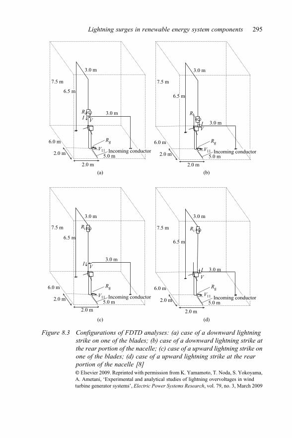
3.0 m

3.0 m

3.0 m

3.0 m

3.0 m 3.0 m

VI

Rg

Rg Rg

6.0 m

6.0 m 6.0 m

5.0 m

5.0 m 5.0 m

Ri

Ri Ri

7.5 m

7.5 m 7.5 m

(c) (d)

(a) (b)

2.0 m

2.0 m 2.0 m

2.0 m

2.0 m 2.0 m

6.5 m

6.5 m6.5 m

V11

V11 V11

VI

VI

3.0 m

3.0 m

Rg

5.0 m

Ri

7.5 m

2.0 m

V11

VI

6.0 m

2.0 m

6.5 m

Incoming conductor Incoming conductor

Incoming conductor Incoming conductor

Figure 8.3 Configurations of FDTD analyses: (a) case of a downward lightningstrike on one of the blades; (b) case of a downward lightning strike atthe rear portion of the nacelle; (c) case of a upward lightning strike onone of the blades; (d) case of a upward lightning strike at the rearportion of the nacelle [8]� Elsevier 2009. Reprinted with permission from K. Yamamoto, T. Noda, S. Yokoyama,A. Ametani, ‘Experimental and analytical studies of lightning overvoltages in windturbine generator systems’, Electric Power Systems Research, vol. 79, no. 3, March 2009


as follows: when current is injected at the tip of the blade equipped with the parallellightning conductor, the current propagates along the lightning conductor. Duringthis process, the intensity of the electric and magnetic fields generated around thelightning conductor increases, resulting in an increase in the voltage at the tip ofthe blade. After the traveling wave reaches the nacelle, the surge impedance of thenacelle becomes smaller than that of the lightning conductor; therefore, a negativereflection is caused at the nacelle, and the negative traveling wave returns to the tipof the blade. The electric and magnetic fields around the blade start weakening;further, the voltage at the tip attains its peak value when the negative reflectedwave reaches the tip again. Since the return propagation time of the blade is 5 ns,the peak of the voltage appears after approximately 5 ns. The surge impedance ofthe tower mainly influences the second peak of the voltage at approximately 17 ns,and the traveling waves on the lightning conductors that have an open end aresuperimposed on the voltage. Meanwhile, the voltage waveforms in Figures 8.5 and8.7 can be explained as follows: as soon as current is injected into the rear portion

(a)

(b)

0 5 10 15 20

0 5 10 15 20–0.5

0

0.5

1

1.5

Time (ns)

Cur

rent

(A)

Measured resultCalculated result

–100

0

100

200

300

400

Time (ns)

Vol

tage

(V)


Figure 8.4 Current I (a) and voltage V (b) at the lightning-strike point underthe conditions of downward lightning, tip of blade, Rg ¼ 9.4 W, andt¼ 4 ns [8]� Elsevier 2009. Reprinted with permission from K. Yamamoto, T. Noda, S. Yokoyama,A. Ametani, ‘Experimental and analytical studies of lightning overvoltages in windturbine generator systems’, Electric Power Systems Research, vol. 79, no. 3, March 2009


of the nacelle, the traveling wave disperses to the three blades and the tower.Because these surge impedances are connected in parallel, the voltage rise is smallfor 5 ns. After 5 ns, the positive traveling waves return to the nacelle from the tipsof the blades, and the voltage at the rear portion of the nacelle starts increasingbecause of the current flow through the tower. The voltage rise exhibits a peakwhen the negative traveling wave at the tower foot reaches the nacelle (afterapproximately 11 ns).

In both upward and downward lightning, the shapes of the voltage curves arealmost the same, as shown in Figures 8.4–8.7. However, the magnitudes in boththese conditions are different because a part of the traveling wave from above isreflected to the upper current lead wire, while a part of it permeates through the WTin the case of upward lightning.

The results calculated using the FDTD for Rg ¼ 0 W, 9.4 W, and 20 W areshown in Figure 8.8. The voltage waveforms obtained for Rg ¼ 0 W, 9.4 W, and20 W change after approximately 17 ns because the reflected wave at the tower foot

(a)

(b)

0 5 10 15 20–0.5

0

0.5

1

1.5

Time (ns)

Cur

rent

(A)


0 5 10 15 20–100

0

100

200

300

400

Time (ns)

Vol

tage

(V)


Figure 8.5 Current I (a) and voltage V (b) at the lightning-strike point underthe conditions of downward lightning, rear portion of a nacelle,Rg ¼ 9.4 W, and t¼ 4 ns [8]� Elsevier 2009. Reprinted with permission from K. Yamamoto, T. Noda, S. Yokoyama,A. Ametani, ‘Experimental and analytical studies of lightning overvoltages in windturbine generator systems’, Electric Power Systems Research, vol. 79, no. 3, March 2009


is different in each condition. The calculation results for t¼ 4 ns, 10 ns, 20 ns, and60 ns are shown in Figure 8.9. In the case of downward lightning at the top of theblade, the second peak of V becomes larger than its first peak when the wave frontof the injected current becomes large.

8.1.1.4 Overvoltage caused by potential riseV11 to V14 in Figure 8.10 represent the voltage difference between the tower foot andthe incoming conductor directed from a distant point and earthed at the remote end;depending on the earthing resistance, this voltage difference is caused by the voltageincrease at the tower foot. In particular, the voltage difference produces an over-voltage between a power line and a power converter or a transformer installed insidethe tower on the earth level, or that between a communication line and a tele-communication device. The incoming conductor is an insulated copper wire orcoaxial cable traced on the aluminum plate from a distant point and earthed at the

0 5 10 15 20–0.5

0

0.5

1

1.5

Time (ns)

Cur

rent

(A)


(a)

(b)

0 5 10 15 20–100

0

100

200

300

400

Time (ns)

Vol

tage

(V)


Figure 8.6 Current I (a) and voltage V(b) at the lightning-strike point underthe conditions of upward lightning, tip of blade, Rg ¼ 9.4 W, andt¼ 4 ns [8]� Elsevier 2009. Reprinted with permission from K. Yamamoto, T. Noda, S. Yokoyama,A. Ametani, ‘Experimental and analytical studies of lightning overvoltages in windturbine generator systems’, Electric Power Systems Research, vol. 79, no. 3, March 2009


remote end. The length of the conductors is 4.5 m. The large earth capacitance of thetraced conductor is comparable to that of the underground cables in actual WTs.

The experimental and calculation results are shown in Figure 8.11 under theconditions of downward lightning, top of the blade, Rg ¼ 9.4 W, and t¼ 4 ns. Inthe FDTD analyses, it is difficult to model a coaxial cable because a side of thecube cells that is part of the FDTD space is not sufficiently larger than the radius ofthe coaxial cable. In this FDTD analysis, only V11 is calculated. V11 to V13 becomenearly identical to the waveform shown in Figure 8.11. The same tendency isobserved in the other conditions. The potential of the insulated copper wire and themetal sheath of the coaxial cable become nearly equal because they are connectedto the aluminum plate at the remote end. Therefore, there is no large differencebetween V11 and V12. The potential of the core of the coaxial cable becomes nearlyequal to that of the metal sheath that covers the core. Therefore, the differencebetween V12 and V13 is not significant. In order to suppress the overvoltage betweenthe incoming conductor and the tower foot, the metal sheath of the coaxial cable is

(a)

(b)

0 5 10 15 20–0.5

0

0.5

1

1.5

Time (ns)

Cur

rent

(A)

0 5 10 15 20–100

0

100

200

300

400

Time (ns)

Vol

tage

(V)



Figure 8.7 Current I (a) and voltage V (b) at the lightning-strike point underthe conditions of upward lightning, rear portion of a nacelle,Rg ¼ 9.4 W, and t¼ 4 ns [8]� Elsevier 2009. Reprinted with permission from K. Yamamoto, T. Noda, S. Yokoyama,A. Ametani, ‘Experimental and analytical studies of lightning overvoltages in windturbine generator systems’, Electric Power Systems Research, vol. 79, no. 3, March 2009


connected to the earth of the tower foot. The voltage difference V14 in such case issuppressed, 40–80%, as compared with V13.

The relations between the maximum value of V11 to V13 and t under the condi-tions Rg ¼ 0 W, 9.4 W, and 20 W are shown in Figure 8.12. The relations between themaximum values of V11 to V13 and Rg under the conditions t¼ 4 ns, 10 ns, 20 ns, and60 ns are shown in Figure 8.13. The maximum value of V11 to V13 decreases with anincrease in t and is proportional to Rg. Moreover, in the case of Rg ¼ 0 W, the max-imum value of V11 to V13 becomes 12 V/A, which is caused by the electromagneticinduction from the current following through the tower and aluminum plates.

The same tendency is observed in the relations between the maximum valueof V14 and t and that between the maximum value of V14 and Rg. In the case ofRg ¼ 0 W, the maximum value of V14 becomes 5.9 V/A.

8.1.2 Earthing characteristics of a wind turbineDamage caused to WTs due to lightning affects the safety and reliability of thesesystems. Most of the breakdowns and malfunctions of the electrical and controlsystems inside or in the vicinity of WTs are caused by earth potential rise due to

1.5

1

0.5C

urre

nt (A

)Vo

ltage

(V)

0

–0.5

400

300

200

100

0

–100

0 5 10Time (ns)

20 Ω

0 Ω

15 20

0 5 10Time (ns)

15 20

20 Ω

0 Ω

(a)

(b)

Figure 8.8 Relations between V, I, and Rg under the conditions of downwardlightning, top of the blade and t¼ 4 ns: (a) current I from FDTDanalytical results; (b) voltage V from FDTD analytical results [8]� Elsevier 2009. Reprinted with permission from K. Yamamoto, T. Noda, S. Yokoyama,A. Ametani, ‘Experimental and analytical studies of lightning overvoltages in windturbine generator systems’, Electric Power Systems Research, vol. 79, no. 3, March 2009


lightning [4, 8, 12]. To solve the mechanism of generation of the potential rise inthese multifarious earth systems, impulse tests at many kinds of WT sites arenecessary [13–27].

In this section, the measurements of transient earthing characteristics carriedout at WTs [13–26] are described. Some of the measured earthing characteristicshave already been verified [17–26] using the FDTD method. From these comparedresults, it has been obvious that these earthing characteristics can be simulated bythe FDTD method accurately.

8.1.2.1 Measurement sitesThe measurements of earthing characteristics of WTs have been completed at the 11sites shown in Figure 8.14. The relations between lightning current characteristic andovervoltage on electrical and electronics equipment at each site have been clarified.Sites 1–5 are in winter lightning area around the Sea of Japan and Sites 6–11 are insummer lightning area. At most of the sites, the lightning current waveforms had beenrecorded using Rogowski coils whose frequency band is about 0.1 Hz to 1 MHz [5–7].

(a)

(b)

1.54 ns

4 ns

10 ns

10 ns

20 ns

20 ns

60 ns

60 ns

1

0.5

Cur

rent

(A)

Volta

ge (V

)0

–0.5

400

300

200

100

0

–100

0 5 10Time (ns)

15 20

0 5 10Time (ns)

15 20

Figure 8.9 Relations between V, I, and t under the conditions of downwardlightning, top of the blade, and Rg ¼ 9.4 W: (a) current I from FDTDanalytical results; (b) voltage V from FDTD analytical results [8]� Elsevier 2009. Reprinted with permission from K. Yamamoto, T. Noda, S. Yokoyama,A. Ametani, ‘Experimental and analytical studies of lightning overvoltages in windturbine generator systems’, Electric Power Systems Research, vol. 79, no. 3, March 2009


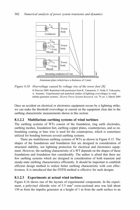
Once an accident on electrical or electronics equipment occurs by a lightning strike,we can make the threshold overvoltage or current on the equipment clear due to theearthing characteristic measurements shown in this section.

8.1.2.2 Multifarious earthing systems of wind turbinesThe earthing systems of WTs consist of the foundation, ring earth electrodes,earthing meshes, foundation feet, earthing copper plates, counterpoises, and so on.Insulating coating or bare wire is used for the counterpoise, which is sometimesutilized for bonding between several earthing systems.

There are multifarious earthing systems of WTs as shown in Figure 8.15. Theshapes of the foundations and foundation feet are designed in consideration ofstructural stability, not lightning protection for electrical and electronics equip-ment. However, the earthing characteristic of a WT depends on the shapes of thesefoundations and foundation feet considerably. The author is afraid that there arefew earthing systems which are designed in consideration of both transient andsteady-state earthing characteristics efficiently. It should be important to establishefficient design method to realize better earthing characteristic with cost effec-tiveness. It is introduced that the FDTD method is effective for such designs.

8.1.2.3 Experiments at actual wind turbinesFigure 8.16 shows one of the layouts of experimental components. In the experi-ment, a polyvinyl chloride wire of 5.5 mm2 cross-sectional area was laid about150 m from the impulse generator at a height of 1 m from the earth surface to an

Incoming conductor (4.5 m)

Aluminum plate (which have a thickness of 2 mm)

CoreSheath

V12

V13

Towerbody

Conductor

V11

Towerbody

V14 TowerbodyCore

Sheath

Figure 8.10 Overvoltage caused by voltage rise of the tower foot [8]� Elsevier 2009. Reprinted with permission from K. Yamamoto, T. Noda, S. Yokoyama,A. Ametani, ‘Experimental and analytical studies of lightning overvoltages in windturbine generator systems’, Electric Power Systems Research, vol. 79, no. 3, March 2009


area near the point of current injection (at the tower foot of the WT), and wasconnected to the foundation through a resistor of 500 W (resistance that is suffi-ciently greater than the earthing impedance of the WT). By injecting current intothe foundation through the resister of 500 W, the impulse generator is regarded as asource of current and steep wave front current can be injected. The current withsteep front of about 40 A in peak value and about 0.2 ms in wave front duration wasinjected as shown in Figure 8.17. Such steep front current contains wide frequencyband components. Once a time-domain response such as a potential rise of anearthing system is measured, wide frequency characteristic can be obtained.

The measured potential rise is the potential difference between the voltage mea-suring wire earthed at a remote point and the foundation. Since the surge impedance ofthe voltage reference line is about 400 W, the sum of the earth resistance value of theearthing electrode at the remote end of the voltage measuring wire and the value of amatching resistor inserted between the voltage measuring wire and the earthing elec-trode at the remote end is adjusted to the value of 400 W. This enables various types ofnoise induced in the voltage reference line to be discharged to the earth smoothly.

(a)

(b)

50

40

30

20

10Volta

ge (V

)0

–100 5 10 15

Time (ns)

Time (ns)

20 25 30 35

V11–V13V14

50

40

30

20

Volta

ge (V

)

10

0

–100 5 10 15 20 25 30 35

V11

Figure 8.11 Voltage differences between the incoming conductor and the towerfoot under the conditions of downward lightning, top of the blade,Rg ¼ 9.4 W, and t¼ 4 ns: (a) voltage V11–V14 of measured results;(a) voltage V11 of FDTD analytical results [8]� Elsevier 2009. Reprinted with permission from K. Yamamoto, T. Noda, S. Yokoyama,A. Ametani, ‘Experimental and analytical studies of lightning overvoltages in windturbine generator systems’, Electric Power Systems Research, vol. 79, no. 3, March 2009


As shown in Figure 8.16, the current lead and the voltage measuring wires arenot orthogonal in some experiments because of restrictions of available space forexperiments. If the angle is less than 90 degrees, inductive effects appear on thevoltage measuring wire, and the measured result of the potential rise may not becorrect. However, most of the results are verified using the FDTD method and we

50

Rg = 0 ΩRg = 9.4 ΩRg = 20 Ω

Rg = 0 ΩRg = 9.4 ΩRg = 20 Ω

Rg = 0 ΩRg = 9.4 ΩRg = 20 Ω

Rg = 0 ΩRg = 9.4 ΩRg = 20 Ω

40

30

20

Volta

ge (V

)

10

0

–10

50

40

30

20

Volta

ge (V

)

10

0

–10

50

40

30

20

Volta

ge (V

)

10

0

–10

50

40

30

20

Volta

ge (V

)

10

0

–100 10 20 30

Wavefront (ns)40 50 60 70

0 10 20 30Wavefront (ns)

40 50 60 70 0 10 20 30Wavefront (ns)

40 50 60 70

0 10 20 30Wavefront (ns)

40 50 60 70

(a) (b)

(c) (d)

Figure 8.12 Relations between the maximum values of V11 to V13 and t: (a) caseof the downward lightning and stroke at the top of the blade;(b) case of the downward lightning and stroke at the rear portion ofthe nacelle; (c) case of the upward lightning and stroke at the top ofthe blade; (d) case of the upward lightning and stroke at the rearportion of the nacelle [8]� Elsevier 2009. Reprinted with permission from K. Yamamoto, T. Noda, S. Yokoyama,A. Ametani, ‘Experimental and analytical studies of lightning overvoltages in windturbine generator systems’, Electric Power Systems Research, vol. 79, no. 3, March 2009


estimate the induction level. From those comparisons between measurements andsimulations, it has been obvious that influence of up to 30% appears on the mea-sured results of the potential rise.

When the steep wave front current such as that shown in Figure 8.17 is injectedinto earthing systems, the potential rise at all sites shows inductive potential, as can

50

(a) (b)

(c) (d)

40

30

20

Volta

ge (V

)

10

0

–100 10

Grounding resistance (Ω)

τ = 4 nsτ = 10 nsτ = 20 nsτ = 60 ns

τ = 4 nsτ = 10 nsτ = 20 nsτ = 60 ns

τ = 4 nsτ = 10 nsτ = 20 nsτ = 60 ns

τ = 4 nsτ = 10 nsτ = 20 nsτ = 60 ns

20

50

40

30

20

Volta

ge (V

)

10

0

–100 10

Grounding resistance (Ω)20

50

40

30

20

Volta

ge (V

)

10

0

–100 10


50

40

30

20

Volta

ge (V

)

10

0

–100 10


Figure 8.13 Relations between the maximum values of V11 to V13 and Rg: (a) caseof the downward lightning and stroke at the top of the blade; (b) caseof the downward lightning and stroke at the rear portion of thenacelle; (c) case of the upward lightning and stroke at the top of theblade; (d) case of the upward lightning and stroke at the rear portionof the nacelle [8]� Elsevier 2009. Reprinted with permission from K. Yamamoto, T. Noda, S. Yokoyama,A. Ametani, ‘Experimental and analytical studies of lightning overvoltages in windturbine generator systems’, Electric Power Systems Research, vol. 79, no. 3, March 2009


be seen in Figure 8.14. The values of earthing resistance of WTs have to be lessthan 10 W [2]. In such a low earthing resistance facility, it is common thatthe inductive potential rise appears. Some typical results of the potential rise areshown in Figure 8.18. The steady-state earthing resistance can be calculated usingthe wave tail values of the injected current and the potential rise waveforms. Themaximum value of the transient earthing impedance can be calculated usingthe wave front values of the injected current and the potential rise waveforms. Interms of lightning protection, both the values of transient earthing impedance andthe steady-state earthing resistance become important. Specially, the former andlatter are important for WTs constructed at summer and winter lightning area,respectively.

It is also obvious that the potential rise depends on the stratified earth resis-tivity at each WT site. High-frequency components of the injected current in thewave front propagate near the earth surface. The depth which depends on the fre-quency f of the injected current, soil permeability m, and resistivity r is calculatedapproximately as follows:

d ¼ffiffiffiffiffiffiffiffir

pf m

rð8:1Þ

If low-resistivity layer exists at near surface, surge can propagate easily. Itmeans that the potential rise at the wave front becomes lower. The stratiform earthresistivity at each site is measured using the Wenner method. Please see the detailsshown in [18].

Test sites

Figure 8.14 Measurement sites of wind turbine earthing characteristics


8.1.2.4 Simulations using the FDTD methodIn some sites shown in Figure 8.14, reproductions of measurements have been doneusing the FDTD method. Good agreements between measured and simulatedresults as shown in Figure 8.19 have been realized. Lately, the modeling methodsof the WTs are introduced in several technical papers [17–26], and high accuracysimulations have become possible.

8.1.2.5 Frequency characteristics of wind turbinesOnce the injected current and potential rise waveforms such as that shown inFigures 8.17–8.19 have been specified, the frequency characteristics of the earthingsystem as shown in Figure 8.20 can be calculated by using the Laplace transform.From the frequency characteristics of the absolute and phase values of the earthingimpedance, the time responses to all the different lightning wave shapes can becalculated. As examples, potential rise responses to a step current with a peak value

Needly electrode

0.5 m

Needly counterpoise

2.675 m

Groundingmesh

1.35 mSide view4.3 m

15.1 m

6.5 m

Top view

Groundingmesh

4.0 m

4.0 m

(a)

3 m

2 m

8.5 m

Grounding meshFoundationfoot: 50 m

Grounding mesh

0.3 m

4.25 m

Top view

Side view

Bottom view

Foundation

(b)4 m

2.8 m

14 m

0.5 m

6 m

0.5 m

Grounding wireGrounding copper plate

(c)

Figure 8.15 Multifarious earthing systems of wind turbines: (a) earthing system ofSite 3; (b) earthing system of Site 6; (c) earthing system of Site 9 [27]� IEEE 2012. Reprinted with permission from Yamamoto, K., Yanagawa, S., ‘Transientgrounding characteristics of wind turbines’, IEEE Proceedings, September 2012


of 1 A and a typical lightning current with a peak value of 30 kA, the wave front of5.5 ms, and the stroke duration of 75 ms are shown in Figure 8.21. By the way, theabove-mentioned measured results do not include the influence of surge propaga-tions at the tower and blades; they are the independent and pure characteristics ofthe earthing system, because the frequency characteristics of Figure 8.20 have beencalculated from the FDTD simulation without the tower and blades.

8.1.3 Example of lightning accidents and its investigationsIn this section, lightning protection studies for a wind farm are introduced [26]. InTaikoyama Wind Farm constructed in the north part of Kyoto Prefecture and nearthe Sea of Japan, WTs have often been damaged by lightning in winter. To solvethe problem and build lightning protection methodologies, a meeting of the com-mittee had been convened from March 2003; many professionals of lightningprotection and WTs had joined. As a result of the discussions at the meeting, alightning protection tower was built near one of the WTs in December 2003. Afterthe construction of the lightning protection tower, many lightning discharges havebeen caught by the tower; the efficiency of the tower has been recognized.

In the winter from 2011 to 2012, two typical accidents have occurred. In one ofthe accidents, a fire occurred inside the WT close to the lightning protection toweron January 28, 2012. Hereinafter, this accident is called ‘‘Accident 1.’’ Accident 1has been caused by a lightning to the WT itself; a back-to-back (BTB) convertersystem has remarkably burned out. Another accident has been the breakdown of theanemometers placed on the lightning protection tower on March 24, 2012. Here-inafter, this accident is called ‘‘Accident 2.’’

In this section, the causes and the protection methodologies for these accidentshave been introduced. To confirm reliability of the protection methods,

V

I

Ground

Foundation

Current lead wire150 m

I.G.

Voltage measuring wire70 m

Figure 8.16 Experimental set-up at Site 6 [27]� IEEE 2012. Reprinted with permission from Yamamoto, K., Yanagawa, S., ‘Transientgrounding characteristics of wind turbines’, IEEE Proceedings, September 2012


experiments of transient earthing characteristics and simulations using the FDTDmethod have been done. From comparison of these results, the degree of con-fidence in the simulation model can be testified, and the level of overvoltages at theWT and the lightning protection tower can be understood.

0

10

20

30

40

50

60

0 5 10 15 20 25 30 35

Cur

rent

(A)

Time (μs)

Time (μs)

Time (μs)

(a)

(b)

(c)

0

20

40

60

80

0 1 2 3 4 5

Cur

rent

(A)

0

10

20

30

40

0 2 4 6 8 10

Cur

rent

(A)

Figure 8.17 Typical injected current waveforms: (a) injected current waveform atSite 3; (b) injected current waveform at Site 6; (c) injected currentwaveform at Site 9 [27]� IEEE 2012. Reprinted with permission from Yamamoto, K., Yanagawa, S., ‘Transientgrounding characteristics of wind turbines’, IEEE Proceedings, September 2012


8.1.3.1 Situations of the accidentsAccident 1 has unfortunately occurred during anemometer installations; thoseanemometers were planned to be set up at the height of 49.7 m, 81 m, and 93.7 m asshown in Figure 8.22. Metal wires of control and power lines are connected to thethree anemometers and lead to the inside of the nearby WT by way of the con-nection box around the foot of the lightning protection tower. The details of the

(a)

(c)

(b)

–500

50100150200250300

0 5 10 15 20 25 30 35

Vol

tage

(V)

Time (μs)

–100

0

100

200

300

400

500

0 1 2 3 4 5

Vol

tage

(V)

Time (μs)

Time (μs)

–1000

100200300400500600

0 2 4 6 8 10

Vol

tage

(V)

Figure 8.18 Typical potential rise waveforms: (a) potential rise waveform atSite 3; (b) potential rise waveform at Site 6; (a) potential risewaveform at Site 9 [27]� IEEE 2012. Reprinted with permission from Yamamoto, K., Yanagawa, S., ‘Transientgrounding characteristics of wind turbines’, IEEE Proceedings, September 2012


circuit of the anemometer system involved in Accident 1 are shown in Figure 8.23(a).When lightning strike the WT, potential rise of the WT foundation occurred as shownin Figure 8.24. It can be guessed that the potential rise caused discharges between themetal wire lead from the lightning protection tower and earthed parts inside the WT[12]; finally the discharges gave rise to the fire. The pictures of Accident 1 are shownin Figure 8.25.

After Accident 1, the set-up of the anemometer system was finished. The circuitof the system is shown in Figure 8.23(a). The system didn’t have an enough lightningprotection system. Therefore, there was possibility of breakdowns of anemometersand other equipment. Lightning to the lightning protection tower caused voltage

(a)

(b)

(c)

(d)

(e)

(f)

0

10

20

30

40

0 5 10 15 20 25 30 35

Cur

rent

(A)

Time (μs) Time (μs)

Simulation

Experiment

–500

50100150200250300

0 10 20 30

Volta

ge (V

)

Time (μs)

Time (μs) Time (μs)

Time (μs)

SimulationExperiment

0

20

40

60

80

0 1 2 3 4 5

Cur

rent

(A)

FDTD calculation

Measurment

–1000

100200300400500

0 1 2 3 4 5

Volta

ge (V

)

FDTD calculation

Measurment

0

10

20

30

40

0 2 4 6 8 10C

urre

nt (A

)

Experiment

Simulation

–1000

100200300400500600700

0 2 4 6 8 10

Volta

ge (V

)

Simulation

Experiment

Figure 8.19 Comparisons between measurements and FDTD simulations:(a) injected current waveform at Site 3; (b) potential rise waveformat Site 3; (c) injected current waveform at Site 6; (d) potentialrise waveform at Site 6; (e) injected current waveform at Site 9;(f) potential rise waveform at Site 9 [27]� IEEE 2012. Reprinted with permission from Yamamoto, K., Yanagawa, S., ‘Transientgrounding characteristics of wind turbines’, IEEE Proceedings, September 2012


difference between the structures of the lightning protection tower and power andsignal lines leading to the anemometers. Breakdowns have occurred at the weakestpoint. The breakdown point is shown in Figure 8.26, where a spark track can be seen.

8.1.3.2 Protection methodologiesTo prevent these accidents, the protection system shown in Figure 8.23(b) wasproposed. In the protection system, anemometer system is gathered at the side ofthe lightning protection tower; there is no metal wire between the lightning pro-tection tower and the WT. However, this system could not be established at sitebecause of its higher cost exceeding the budgetary limits. Instead, the protectionsystem using potential equalization method shown in Figure 8.23(c) was set up.

The concept of the protection system shown in Figure 8.23(b) is ‘‘isolation’’between the lightning protection tower and the nearby WT. However, electro-optic

(a)

(b)

0

5

10

15

20

25

30

104 105 106 107

Impe

danc

e (Ω

)

Frequency (Hz)

0102030405060708090

104 105 106 107

Phas

e (d

egre

e)

Frequency (Hz)

Figure 8.20 Frequency responses of the earthing system at Site 6: (a) absolutevalue of the earthing impedance; (b) phase value of the earthingimpedance [18]� 2010 IEEE. Reprinted with permission from Yamamoto, K., Yanagawa, S.,Yamabuki, K., Sekioka, S., Yokoyama, S., ‘Analytical surveys of transient and frequency-dependent grounding characteristics of a wind turbine generator system on the basis offield tests’, IEEE Transactions on Power Delivery, vol. 25, no. 4, October 2010


–202468

101214161820

0 2 4 6 8 10

Vol

tage

(V)

Time (μs)

Time (μs)

(a)

(b)

(c)

05

101520253035

0 5 10 15 20

Time (μs)0 5 10 15 20

Cur

rent

(kA

)

010203040506070

Vol

tage

(kV

)

Figure 8.21 Potential rise response to step and typical lightning currents atSite 6: (a) potential rise response to a step current; (b) typicallightning current waveform; (c) potential rise response to the typicallightning current [18]� 2010 IEEE. Reprinted with permission from Yamamoto, K., Yanagawa, S.,Yamabuki, K., Sekioka, S., Yokoyama, S., ‘Analytical surveys of transient and frequency-dependent grounding characteristics of a wind turbine generator system on the basis offield tests’, IEEE Transactions on Power Delivery, vol. 25, no. 4, October 2010


conversion equipment is utilized and an independent source is needed. Becausethis system costs a lot, the system could not be installed. On the other hand, theconcept of the protection system shown in Figure 8.23(c) is ‘‘potential equaliza-tion.’’ To decrease the lightning current into the metal wires such as control andpower lines, earthing wires between the lightning protection tower and the nearbyWT are set up.

8.1.3.3 Measurements and simulations of transient earthingcharacteristic

To confirm reliability of the protection methods shown in Figure 8.23(c), the authorhas a plan to make a simulation model using the FDTD method. For the validationof the FDTD model, the earthing potential rises and shunt currents are compared onthe FDTD simulations and the measurements.

Figures 8.27 and 8.28 show the earthing wires between the foundation of WTand the lightning protection tower, and the details of the WT earthing system. Theearthing resistivity has been measured by using the Wenner method. Figures 8.29and 8.30 show the layer of earthing resistivity around the test site and the

(a) (b)

49.7

m31

.3 m

12.7

m

104

m

Vaneanemometer

Lightning rod

1.7 m

13.0 m 7.0 m

1.0 m2.0 m 2.5 m

Underground beamwidth 0.7 mheight 2.0 m

Plate-type groundingelectrode

0.9 m × 0.9 m

Ring earth electrode

9.0

m

7.0

m2.5 m

Figure 8.22 Details of the lightning protection tower: (a) overall view;(b) earthing system [26]� IEEE 2013. Reprinted with permission from Yamamoto, K., Sumi, S., ‘Validationsof lightning protections for accidents at a wind farm’, IEEE Proceedings, October 2013


measuring place of the Wenner method. Based on the experimental set-up shown inFigure 8.31, the transient characteristic of the earthing system has been measured.

In the analysis, the experiment layout is expressed as faithfully as possibleusing analytical spaces as shown in Figure 8.32. The shape of the analytical space isrectangular, with 166 m in the x direction, 141 m in the y direction, and 124 m inthe z direction, and grid spacing is all set to 0.5 m. Six faces that surround theanalytic spaces have an open space simulated using the Liao’s second-orderabsorbing boundary condition. The earth in the experiment is expressed by fillingthe space with the substance of resistivity r¼ 17.8 Wm and relative permittivity 10with 18 m high from the bottom of the analytic space, then, over the top of it, fillingthe space with the substance of resistivity r¼ 427 Wm and relative permittivity10 with 5 m thickness high.

Voltageconverter ELC

Measurementdevice

Distribution board(at wind turbine)

Distribution board(at the bottom of the lightning

protection tower)

Vane anemometerNo.1

No.2

No.3

January 25, 2012: OpenMarch 24, 2012: Close

PC

Current signal (4–20 mA):

Underground wire

Lightningprotection tower

No.1

No.2

No.3

Wind turbinegenerator

Communication line(Insulating covered wire)

Power line100 V

Com. line (Ground line)

SPD


SPD

ELCSPD

Power line24 V

100 V

(a)


SPD

Figure 8.23 Wire diagram of anemometer system: (a) wire diagram at accidents;(b) recommended lightning protection system; (c) adopted lightningprotection system [26]� IEEE 2013. Reprinted with permission from Yamamoto, K., Sumi, S., ‘Validationsof lightning protections for accidents at a wind farm’, IEEE Proceedings, October 2013


The polyvinyl chloride wires are used for the current lead wire and the voltagemeasuring wire; earthing wires are expressed by thin wire model with actual radiusof those wires. The foundation and plate-type earthing electrodes are simulated asperfect conductors. The WT near the lightning protection tower is connected withother WTs by counterpoises. It is impossible to model all WTs in the wind farm in asame FDTD analytical space because of shortage of performance of personalcomputers. In this simulation model, the earthing system of other WTs is modeledas a perfect conductor of 100 m � 20 m � 30 m.

The injected current in the analysis is set to be the same as that of theexperimental result shown in Figure 8.33. The current is injected to the top of thefoundation via 500 W resistance. In order to identify transient earthing

(b)

Vane anemometer


No.1

No.2

No.3

Power line

Optical signal :

Communication line(optical cable)

SPD

SPD

SPD

ELB

DC: 24 V

AC: 100 VPC

No.1

No.2

No.3

SPD

SPD

SPD

SPD box(grounded to the towerstructure near the vain

anemometer)

Voltageconverters

Distribution board(at the bottom of the lightning protection tower )

Measurementdevice

Figure 8.23 (Continued)


characteristics of the WT, current that flows into the foundation, the potential riseof the foundation, and the shunt current through the earthing wires between the WTand the lightning protection tower have been calculated.

The comparisons between experimental and simulation results are shown inFigures 8.33–8.35. The current shown in Figure 8.33 has been injected and thepotential rise at the foundation of the WT in Figure 8.14 has been measured andcalculated in the cases that the earthing system of the lightning protection tower isconnected and disconnected with that of the nearby WT. Figure 8.35 shows theshunt currents into three connection earthing wires. The waveform of the totalshunt current is shown in Figure 8.35(c); compared with the injected current, themaximum shunt current has become over 40% of the injected current. From theabove-mentioned results, we can get good agreements between experimental andsimulation results.

After the completion of the FDTD model, overvoltage and shunt current atsurge protective devices (SPDs) in the anemometers are simulated. From theseresults, the lightning protection efficiencies can be confirmed.

Measurementdevice

Distribution board(inside of the wind turbine)

Distribution board(at the bottom of the lightning

protection tower) Vane anemometer

No.1

No.2

No.3

Power line

Communication line

100 V

PC

Current signal (4–20 mA):

Underground wire(c)

Voltage signal (1–5 V):

SPDSPD

SPD

SPD

Signalconverter

SPD

Signalconverter

SPD

Voltageconverter

ELBMCCB

No.1

No.2

No.3

Wind turbinegenerator


SPD box(at the door of the wind turbine)

DC: 24 V

AC: 100 V

SPD

SPD

SPD

SPD

SPD

SPD

SPD box(grounded to the towerstructure near the vain

anemometer)

SPD

SPD

SPD

SPD

SPD

SPD

To signalconverters

SPD

Signalconverter

SPD

Com. line (Ground line)

Figure 8.23 (Continued)


8.2 Solar power generation system

In recent years, generation methods using renewable energy are rapidly spreadingas a countermeasure of global warming and energy depletion. Large-scale photo-voltaic power plants (PVPPs) are often constructed in the same way as large-scalewind farms.

In such large-scale PVPPs, PV modules are installed on the frame. PVPPs areusually constructed in a large open space where a few tall structures exist to getmore solar energy. Therefore, such large-scale PVPPs are likely to be a target oflightning. To protect them from lightning damages and establish appropriatelightning protections using the lightning rod, surge protective device (SPD) andsuch other devices are required. However, the mechanism of the lightning over-voltage generations has not been well discussed so far [28, 29].

In this section, examples of numerical simulations on PVPPs are introduced.

Potential V

Distance x

Soil

Lightning current

Discharge

Figure 8.24 Discharge caused by the potential rise of the wind turbinefoundation [26]� IEEE 2013. Reprinted with permission from Yamamoto, K., Sumi, S., ‘Validationsof lightning protections for accidents at a wind farm’, IEEE Proceedings, October 2013


8.2.1 Lightning surges in a MW-class solar powergeneration system

In the large-scale PVPPs such as MW-class plants, there are many power con-ditioning systems (PCSs) that are highly capacious and expensive. These expensivefacilities have to be protected from lightning overvoltage.

In this section, at first, the case that lightning overvoltage at the DC side of aPCS has been experimentally studied using the 1/10 scale model is introduced [30].Additionally, the case that the measurements have been verified using the FDTDmethod is explained. Finally, its sensitive analysis depending on the wave frontduration and the earthing resistivity has been introduced.

Figure 8.25 Pictures of the accident: (a) burned-out board of BTB; (b) endterminals of communication and power line leaded from outside [26]� IEEE 2013. Reprinted with permission from Yamamoto, K., Sumi, S., ‘Validationsof lightning protections for accidents at a wind farm’, IEEE Proceedings, October 2013


8.2.1.1 Experiments using the 1/10th scale modelPV array and frame shown in Figure 8.36 are constructed in large open spaceswhere a few tall structures exist. Therefore, these are likely to be a target oflightning. To protect PV modules from direct lightning strikes, sometimes lightningconductors are installed at the top of the frame as shown in Figure 8.37. Whenlightning strikes this lightning conductor, lightning current branches off from thelightning conductor to the frame, then it flows into the earth through the earthingsystem of the PVPP. The lightning conductor is installed on the top of the flame; itsinterval is about 10 cm. It is hard to think that the conductor shows good protectionefficiency for lightning protection because of such interval.

Figure 8.26 Damaged anemometer: (a) appearance of the anemometer; (b) traceof the breakdown discharge [26]� IEEE 2013. Reprinted with permission from Yamamoto, K., Sumi, S., ‘Validationsof lightning protections for accidents at a wind farm’, IEEE Proceedings, October 2013


Lightning often strikes a PV module directly. In such a case, the PV modulestruck by lightning is usually broken, and some PV modules installed near thestruck PV module may also be broken.

In large-scale PVPPs, there are many PCSs that are highly capacious andexpensive. A PCS is set up on each PV array as shown in Figure 8.36.

When lightning strikes the frame supporting PV arrays, surge voltage andcurrent are induced on DC power lines between PV arrays and a PCS and ACpower lines between a PCS and a substation. These induced voltage and currentdepend on the lightning current path on the structure according to the shape of theframe and the earthing system. As a result, overvoltage appears between powerlines and a PCS due to the induced voltage and current, and the potential rise of theearthing system.


Wire 1 (32.7 m)

Wind turbineGrounding

wires

Wire 2 (41.4 m)Wire 3 (32.7 m)

Soil0.6 m

Wind turbine

(a)

(b)

Foundationof wind turbine

Foundation of lightning protection tower

Grounding wires

Wire 1Wire 2

Wire 3

Figure 8.27 Earthing wires between wind turbine foundation and lightningprotection tower: (a) Overhead view; (b) Top view [26]� IEEE 2013. Reprinted with permission from Yamamoto, K., Sumi, S., ‘Validationsof lightning protections for accidents at a wind farm’, IEEE Proceedings, October 2013


17.8 Ωm

4.97 m

∞

427 Ωm

Figure 8.29 Earth resistivity [26]� IEEE 2013. Reprinted with permission from Yamamoto, K., Sumi, S., ‘Validationsof lightning protections for accidents at a wind farm’, IEEE Proceedings, October 2013

1.4 m

13.5 m

1.6 m

0.8 m

4.0 m

4.25 m 5.0 m 4.25 m

16 m

Plate-type grounding electrode0.9 m × 0.9 m Mesh grounding


1.0 m

Plate-type grounding electrode

Mesh grounding


Figure 8.28 Details of wind turbine earthing system [26]� IEEE 2013. Reprinted with permission from Yamamoto, K., Sumi, S., ‘Validationsof lightning protections for accidents at a wind farm’, IEEE Proceedings, October 2013


In this section, at first, the overvoltage appearing at the DC side of the PCS hasbeen experimentally discussed using the 1/10 scale model of the frame structure inthe large-scale PVPPs shown in Figures 8.36 and 8.37. The models of PV modulesare not included in this scale model. The effects of the PV module are ignored, andthe overvoltage that is directly induced to the power line is just considered.

The experimental set-up is shown in Figure 8.38. In this experiment, 1/10 scalemodel of a frame supporting PV arrays in the large-scale PVPP is set up on thealuminum plate of 2 mm in thickness. Current injected points are Point 1 (corner ofthe frame) and Point 2 (center of the frame) shown in Figure 8.38. When current isinjected to these assumed point of the lightning stoke, overvoltage at the DC side(V1, V2 [V]) of the PCS is measured with the injected current (I [A]) at the sametime. The frame shown in Figure 8.38 is made of aluminum pipes whose radius isapproximately 5 mm. The DC power line models are made of polyvinyl chloridewires whose radius is approximately 0.9 mm. The PCS is made of aluminum boxthat is a rectangular parallelepiped conductor, 15 cm on a side.

In general, PCS is installed in the metallic storage box as shown in Figure 8.39.Because this storage box is connected to the earth directly under it, the potential atthe storage box is equal to the earth potential of the installation location. When thepotential at the storage box fluctuates transiently by lightning strike to the frame ofthe supporting PV arrays in the large-scale PVPP, the potential of the PCS in thestorage box also fluctuates with potential at its storage box. As a result, bothpotentials become approximately equal. By such a reason, in this experiment,potential at the PCS installed in the storage box and the potential at the storage boxare dealt as same potential, and the overvoltage between the PCS and power line isdefined as that between the storage box and the power lines.

Locations of the PCS are shown in Figure 8.40(a)–(c). These locations aretypical examples of actual facilities. In Figure 8.40(a), the PCS is installed at the

22.5 m 22.5 m


Ground resistivitymeasuring point

Foundationof lightning protection tower

Grounding wires

Figure 8.30 Measuring point of earth resistivity [26]� IEEE 2013. Reprinted with permission from Yamamoto, K., Sumi, S., ‘Validationsof lightning protections for accidents at a wind farm’, IEEE Proceedings, October 2013


center of the frame, and the PCS gathers electrical power from bilateral PV arrays.In Figure 8.40(b), the PCS is installed at the side of the frame. But the PCS is stillinside of the frame. The PCS is installed at the outside of the frame as shownin Figure 8.40(c). There is the characteristic that the length of the power line inFigure 8.40(b) and (c) is longer than that in Figure 8.40(a).

In the set-up shown in Figure 8.38, coaxial cable (3D2V) connected withthe pulse generator (referred in the figure as P.G.) is laid up over the frame.

I

500 Ω

500 Ω

IV cable

I.G.

I

50 m

50 m

76 mV

Current read wire100 m


Lightning protection tower

(a)

(b)

Grounding wires

Soil0.6 m

Wind turbine

Foundationof lightning protection tower

Grounding wires

I

I

V

I.G.50 m

50 m

76 m

Current lead wire100 m



Figure 8.31 Experimental set-up: (a) Over view; (b) Top view [26]� IEEE 2013. Reprinted with permission from Yamamoto, K., Sumi, S., ‘Validationsof lightning protections for accidents at a wind farm’, IEEE Proceedings, October 2013


The resistance of 500 W is inserted between the frame and the core wire of coaxialcable, and the steep current shown in Figure 8.41 (its peak value and wave frontduration were approximately 1.2 A and 10 ns, respectively) is injected to theframe. The current is injected to the frame, and at the same time the differentpolarity current propagates upward from the injected point on the coaxial cable.

0

5

10

15

20

0 5 10 15 20 25 30 35

Cur

rent

(A)

Time (μs)

Simulation

Experiment

Figure 8.33 Injected current [26]� IEEE 2013. Reprinted with permission from Yamamoto, K., Sumi, S., ‘Validationsof lightning protections for accidents at a wind farm’, IEEE Proceedings, October 2013

Grounding wire(48 m)

VVoltage measurement wire

166 m

I

141 m

Soil

18 m

124 m

5 m17.8 Ωm 427 Ωm

Grounding system model ofother wind turbines

(100 m × 20 m × 3 m)

Current lead wire

Figure 8.32 Analytical set-up [26]� IEEE 2013. Reprinted with permission from Yamamoto, K., Sumi, S., ‘Validationsof lightning protections for accidents at a wind farm’, IEEE Proceedings, October 2013


A part of the current reflects at the curved point of the current lead wire (5 m inheight from the frame), and it returns to the injection point again. This feedbackcurrent influences on the measuring results. In this experiment, the time range of10 m/(3�108 m/s) ffi 30 ns until the reflection wave returns to the injected pointfrom the curved point is validated, because there is no such reflected current inactual lightning phenomenon. The current injection method using such a coaxialcable is explained in [31].

Under these conditions, the experiments of Cases 1.A–2.C shown in Table 8.1have been conducted. Measuring data are the injected current I [A] and thepotential difference between the PCS and DC power line V1, V2 [V].

The voltage waveforms of V1 and V2 in Cases 1.A–2.C are shown inFigures 8.42 and 8.43. In such experiments, the position of the voltage probe cablegreatly influences the experimental results because of the electromagnetic induc-tion from the current flowing on the current lead wire and the frames. To suppresssuch an electromagnetic induction, the voltage probes must be set perpendicularly

0

20

40

60

80

100

Vol

tage

(V)

Simulation

Experiment

0

20

40

60

80

100(a)

(b)

0 5 10 15 20 25 30 35

0 5 10 15 20 25 30 35

Vol

tage

(V)

Time (μs)

Time (μs)

Simulation

Experiment

Figure 8.34 Potential rise at the foundation of the wind turbine (foundationsare disconnected): (a) Connected by three earthing wires;(b) Disconnected [26]� IEEE 2013. Reprinted with permission from Yamamoto, K., Sumi, S., ‘Validationsof lightning protections for accidents at a wind farm’, IEEE Proceedings, October 2013


against all conductors where steep current flows. The distance between conductorsand voltage probes must be larger [12, 32].

However, in these experiments, there is no best set-up that voltage probe cableis placed in vertically against all conductors, because the frame model containsdiagonal bracings. Moreover, the distance between the voltage probe and con-ductors cannot be larger, because the voltage measuring points exist inside theframe. So, in this experiment, the voltage probe cable is extended to the backside ofthe PCS and frame vertically against the current lead wire and the top conductorconsisting the frame. That is the positive direction of the x-axis from the measuringpoint at V1, V2 shown in Figure 8.38.

Next, the amplitude of fluctuations in voltages depending on the position of thevoltage probe is explained. When the angle of the voltage probe cable is changed to10–20 degrees to the y, z direction, voltage fluctuation of 3–5 V occurs. Even ifvoltage probes are set up vertically against all conductors so that steep currentflows on, small induction still remains on it. The induced voltage cannot beremoved completely. I thought that it is because of these reasons the voltage fluc-tuation of 3–5 V occurs.

Because these experimental results are expected to show measurement errors,analyses using the FDTD method have been made in section 8.2.1.2 and the experi-mental results using the scale model are verified. Furthermore, in section 8.2.1.3,analytical studies using an actual-scale FDTD model have been conducted.

00.5

11.5

22.5

33.5

(a) (b)

(c) (d)

0 5 10 15 20 25 30 35

Cur

rent

(A)

00.5

11.5

22.5

33.5

Cur

rent

(A)

Cur

rent

(A)

Cur

rent

(A)

Time (μs)0 5 10 15 20 25 30 35

Time (μs)

0 5 10 15 20 25 30 35Time (μs)

0 5 10 15 20 25 30 35Time (μs)



00.5

11.5

22.5

33.5


0

5

10

15

20


Figure 8.35 Shunt current waveforms: (a) Wire 1; (b) Wire 2; (c) Wire 3; (d) Sumof the currents [26]� IEEE 2013. Reprinted with permission from Yamamoto, K., Sumi, S., ‘Validationsof lightning protections for accidents at a wind farm’, IEEE Proceedings, October 2013


8.2.1.2 Simulations using the FDTD method of the 1/10 scalemodel experiments

The analytical space is shown in Figure 8.44. The scale experiments described insection 8.2.1.1 are verified using this model. The dimension of the analyticalspace is 1.5 m � 5.0 m � 1.6 m and it is divided into cubic cells with a side lengthof 0.01 m. The absorbing boundary condition is the Liao’s second-order condition.

The frame model is installed on the aluminum plate; its resistivity and thick-ness are 2.65 � 10�8 Wm and 2 mm, respectively. This frame model is constructedby using thin wire models [11]. Thin wire models also model the power lines andcurrent lead wire, and the PCS is made of a rectangular parallelepiped conductorand thin wire models. Shape and arrangement of all models shown in Figures 8.38and 8.40 are expressed as faithfully as possible.

The current source and parallel resistance of 500 W are arranged above thecurrent injected point shown in Figure 8.44, and connected between the frame and alightning channel modeled by a thin wire.

As the injected current waveform is approximately equal to that in Figure 8.41,it is omitted in this chapter. In addition, 1 pF capacitor is inserted into the mea-suring point of potential difference because the voltage probe used in the experi-ments has the input capacitance.

Figure 8.36 Solar array of a large-scale photovoltaic power plant [30]� IEEJ 2012. Reprinted with permission from K. Yamamoto, J. Takami, N. Okabe,‘Overvoltages on DC side of power conditioning system caused by lightning strike tostructure anchoring photovoltaic panels’, IEEJ Trans, vol. 132, no. 11, pp. 903–913,November 2012


Under such analytical conditions, the calculations of Cases 1.A–2.C shown inTable 8.1 have been conducted. Output data are the injected current I [A] and thepotential difference between the PCS and DC power line V1, V2 [V].

The potential difference is calculated by multiplying the electric field at thecalculated point by the distance between the PCS and DC power line. The distanceis one cell size in this model. Therefore, the effect of the induced voltage appearedon the voltage probe in the scale model experiments is not contained.

Calculation results of Cases 1.A–2.C are shown in Figures 8.45 and 8.46. Fur-thermore, maximum overvoltage value of each case is summarized in Table 8.2. Asshown in Figures 8.45 and 8.46, the calculation and experimental results have beenqualitatively matched, but a little difference has appeared. The main cause of thedifference is thought to be the induced voltage to voltage probes (cf. section 8.2.1.1).

Approximately 10 ns periodic oscillation is shown in Figures 8.45 and 8.46.This periodic oscillation conforms to the resonant frequency of the conductorsconsisting the frame. The surge current flowing on the conductors reflects andpasses at the connection point, and causes the induced voltage and current on theDC power lines. Finally, the induced voltage becomes the overvoltage at the DCside of the PCS. Moreover, it has been obvious that the effect of induced voltageoccurred by the DC power line working as the dipole antenna [33].

Figure 8.37 Lightning conductor on a structure of a solar array [30]� IEEJ 2012. Reprinted with permission from K. Yamamoto, J. Takami, N. Okabe,‘Overvoltages on DC side of power conditioning system caused by lightning strike tostructure anchoring photovoltaic panels’, IEEJ Trans, vol. 132, no. 11, pp. 903–913,November 2012


In the scale experiments and calculations, the steep current having 10 ns wavefront duration is injected (this wave front duration is equivalent to 0.1 ms in theactual level). This represents very steep wave front duration of an actual subsequentstroke. The wave front duration becomes steeper, and the induced voltage on theDC power line becomes larger.

8.2.1.3 Simulations in case of an actual-scale modelIn this section, at first, the case that the current is injected into the frame supportinga full-scale PV array has been studied. The frame is on the earth where the earth

yxz

Aluminum plate

2 m Point 2

4 m

Power line models(DC sides)

50 cm10 cm

Current lead wire

Power conditioning system model

Coaxial cable

P.G.

V2I

R = 1 kΩ

50 cm80 cm

Point 1

V1

10 m

5 m

5 m

4 m

(a)

(b)

y

z

x


Power line models(DC sides)

Current lead wireI

Aluminum plate

6 cm

10 cm

8 cm

15 cm

15 cm

Figure 8.38 Experimental set-up of the 1/10 scale model of frame supporting PVarrays in a large-scale photo-voltaic power plant: (a) Overall view;(b) Side view [30]� IEEJ 2012. Reprinted with permission from K. Yamamoto, J. Takami, N. Okabe,‘Overvoltages on DC side of power conditioning system caused by lightning strike tostructure anchoring photovoltaic panels’, IEEJ Trans, vol. 132, no. 11, pp. 903–913,November 2012


resistivity is 100 Wm, and the wave front duration of the current is 1 ms. After thatstudy, the overvoltage characteristics dependences on the wave front duration andearth resistivity have been studied.

An analytical model of an actual-scale PVPP is shown in Figure 8.47. Thedimension of the analytical space is 15 m � 50 m � 18 m and it is divided intocubic cells with a side length of 0.1 m. The absorbing boundary condition is theLiao’s second-order condition. The earth level is 7 m from the bottom of the ana-lytical space; the earth resistivity is 100 Wm, and the relative permittivity is 10. Theframe supporting a full-scale PV array is earthed; its earthing resistance isapproximately 3 W. Thin wire models of 5 cm radius compose the frame. Thepower line is also composed by thin wire models of 5 mm radius. The PCS ismodeled as a rectangular parallelepiped conductor of 1.5 m on a side.

The injected current is shown in Figure 8.48. It is a step wave including widefrequency components, and its peak value and wave front duration were approxi-mately 1 A and 1 ms, respectively. Analytical cases are shown in Table 8.1. Otheranalytical conditions are the same as described in section 8.2.1.2.

Calculation results are shown in Figures 8.49 and 8.50. Moreover, maximumovervoltage value is summarized in Table 8.3. Data in Table 8.3 show that the

Figure 8.39 Actual box of a power conditioning system [30]� IEEJ 2012. Reprinted with permission from K. Yamamoto, J. Takami, N. Okabe,‘Overvoltages on DC side of power conditioning system caused by lightning strike tostructure anchoring photovoltaic panels’, IEEJ Trans, vol. 132, no. 11, pp. 903–913,November 2012


120–230 kV overvoltage is applied to PCS DC side when the lightning of the wavefront duration of 1 ms and peak current of 30 kA strikes the frame installed in thelarge-scale PV plant [34].

Next, features of overvoltage waveforms are discussed. In Figures 8.49 and8.50, the oscillation appearing in the waveforms depends on the size of the scale ofthe frame [12, 32].

These oscillated waveforms are also overvoltage occurred by the surge currentreflecting and passing on the frame, and by the DC power lines working as dipole

4 m

Power line models (DC sides)

50 cm

10 cm

50 cm80 cm

V2


V1

Point 1 Point 2

(c)

(b)

(a)

Point 1 Point 2

4 m

Power line model (DC sides)

50 cm

10 cm

50 cm80 cm

V1


Point 1 Point 2

4 m

Power line model (DC sides)

50 cm

10 cm

50 cm80 cm

V1


Figure 8.40 Positions of PCS: (a) Position A; (b) Position B; (c) Position C [30]� IEEJ 2012. Reprinted with permission from K. Yamamoto, J. Takami, N. Okabe,‘Overvoltages on DC side of power conditioning system caused by lightning strike tostructure anchoring photovoltaic panels’, IEEJ Trans, vol. 132, no. 11, pp. 903–913,November 2012


antennas [33]. Especially, the surge current that flows on the conductor existinghorizontally and close to the power line has a significant influence. All overvoltagewaveforms are oscillating in a period of 0.13 ms or 0.27 ms cycle. Those oscillationsare caused because the have half-wave length of each oscillation is equivalent to theapproximate distances of 20 m or 40 m between the current injected point and the endof the frame. In Case 1.A, 0.13 ms periodic oscillations mainly occurred because theDC power line has 20 m length. In Cases 2.A, 2.B, and 2.C, because the length fromcurrent injected point to the end of the frame is also 20 m, 0.13 ms periodic oscillationmainly appeared. On the other hand, in Cases 1.B and 1.C, because the distancebetween the current injected point and the end of the frame is 40 m and the length ofDC power line is 40 m, 0.27 ms periodic oscillation appeared.

The calculation results target the phenomena on the full-scale model, and itsovervoltage has shown the oscillated and inductive waveform with the rise time of

0

0.5

1

1.5

0 5 10 15 20 25 30

Cur

rent

(A)

Time (ns)

Figure 8.41 Injected current into the 1/10 scale model of frame supporting PVarrays in a large-scale photo-voltaic power plant [30]� IEEJ 2012. Reprinted with permission from K. Yamamoto, J. Takami, N. Okabe,‘Overvoltages on DC side of power conditioning system caused by lightning strike tostructure anchoring photovoltaic panels’, IEEJ Trans, vol. 132, no. 11, pp. 903–913,November 2012

Table 8.1 Experimental cases and conditions [30]

Case number Current injected point Position of PCS

1.A Point 1 A1.B Point 1 B1.C Point 1 C2.A Point 2 A2.B Point 2 B2.C Point 2 C

� IEEJ 2012. Reprinted with permission from K. Yamamoto, J. Takami, N. Okabe,‘Overvoltages on DC side of power conditioning system caused by lightningstrike to structure anchoring photovoltaic panels’, IEEJ Trans, vol. 132, no. 11,pp. 903–913, November 2012


approximately 0.5 ms. When lightning strikes the large-scale PVPP, the potential atthe frame supporting PV arrays rises depending on its earthing impedance. As theDC power lines are surrounded by the structures of the frame, the potential of thepower line rises with that of the surrounding space. On the other hand, the potentialof the PCS storage box installed inside the frame and earthed near the frame ismainly affected by the potential rise of the frame foot located closest to the PCSstorage box. It has been thought that V1 and V2 have shown the negative polaritybecause the potential rise of the PCS is higher than that of the DC power linesaround the both wave front and tail. In the study using the scale model, the earthingimpedance of the frame is zero because the frame is directly connected to thealuminum plates spread all over the floor. However, even if the earthing impedanceof the frame is zero, the transient potential rise appears due to electromagneticfields formed around the frame [12, 35, 36]. The results, shown in Figures 8.45 and8.46, in the scale model have indicated the negative polarity due to those reasons.

Sensitive analyses have been done using several different wave front durationsof 0.2, 1.0, 5.5, and 10.0 ms. The analytical conditions in these sensitive analyses arethe same as the previous calculations. Calculation results of Cases 1.A–2.C areshown in Figures 8.51 and 8.52. Maximum and steady-state values of overvoltage

–50–40–30–20–10

01020

(a) (b)

(c) (d)

–5 0 5 10 15 20 25 30

Volta

ge (V

)

Time (ns)

–50–40–30–20–10

01020

–5 0 5 10 15 20 25 30

Volta

ge (V

)

Time (ns)

–50–40–30–20–10

01020

–5 0 5 10 15 20 25 30

Volta

ge (V

)

Time (ns)

–50–40–30–20–10

01020

–5 0 5 10 15 20 25 30

Volta

ge (V

)

Time (ns)

Figure 8.42 Experimental results of V1 and V2 in Cases 1.A�1.B: (a) V1 inCase 1.A; (b) V2 in Case 1.A; (c) V1 in Case 1.B; (d) V1 inCase 1.C [30]� IEEJ 2012. Reprinted with permission from K. Yamamoto, J. Takami, N. Okabe,‘Overvoltages on DC side of power conditioning system caused by lightning strike tostructure anchoring photovoltaic panels’, IEEJ Trans, vol. 132, no. 11, pp. 903–913,November 2012


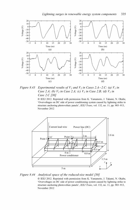
–50–40–30–20–10

01020

–5 0 5 10 15 20 25 30

Vol

tage

(V)

Time (ns)

–50–40–30–20–10

0

0

01020

–5 0 5 10 15 20 25 30

Vol

tage

(V)

Time (ns)(a)

(c)

(b)

(d)

–50–40–30–20–10

1020

–5 0 5 10 15 20 25 30V

olta

ge (V

)

Time (ns)

–50–40–30–20–10

1020

–5 0 5 10 15 20 25 30

Vol

tage

(V)

Time (ns)

Figure 8.43 Experimental results of V1 and V2 in Cases 2.A�2.C: (a) V1 inCase 2.A; (b) V2 in Case 2.A; (c) V1 in Case 2.B; (d) V1 inCase 2.C [30]� IEEJ 2012. Reprinted with permission from K. Yamamoto, J. Takami, N. Okabe,‘Overvoltages on DC side of power conditioning system caused by lightning strike tostructure anchoring photovoltaic panels’, IEEJ Trans, vol. 132, no. 11, pp. 903–913,November 2012

2 mPoint 1

Point 2

4 m

Power line (DC)

I

0.5 m

0.1 m0.5 m

0.8 m

Current lead wire

V2

Power conditioner

V1

5 m

1.5 m

yxz

1.6 m

Figure 8.44 Analytical space of the reduced-size model [30]� IEEJ 2012. Reprinted with permission from K. Yamamoto, J. Takami, N. Okabe,‘Overvoltages on DC side of power conditioning system caused by lightning strike tostructure anchoring photovoltaic panels’, IEEJ Trans, vol. 132, no. 11, pp. 903–913,November 2012


are summarized in Table 8.4. Figure 8.53 shows the relationship diagram betweenthe overvoltage and wave front duration of the injected current.

As described in the previous paragraph in this section, the oscillation includedin the overvoltage waveform is the induced voltage caused by the current flowing onthe frame. Therefore, the wave front duration becomes shorter; the amplitude of theoscillation becomes larger, because the time derivative of the current (dI/dt [A/s])becomes larger. This tendency has been verified in Figures 8.51–8.53. Furthermore,the wave front duration of the injected current gets shorter, and the inductivecharacteristic of the negative potential rise also becomes more sensible. On the otherhand, it is obvious that the influence on overvoltage in the wave tail by the wavefront duration is small.

Table 8.4 and Figure 8.53 represent the quantitative relationship between themaximum and steady-state overvoltage value and the wave front duration. Forexample, in V2 in Case 1.A, 540 kV overvoltage may be applied to the DC side ofthe PCS when the lightning with the wave front duration of 0.2 ms and the peakcurrent of 30 kA strikes the frame constructed on the earth with its resistivity of100 Wm [34]. Because this overvoltage level cannot be ignored on lightning pro-tection designs, it is obvious that establishing the appropriate lightning protectionfor the PCS is important.

–50–40–30–20–10

01020

–5 0 5 10 15 20 25 30

Volta

ge (V

)

Time (ns)(a)

(c) (d)

(b)

–50–40–30–20–10

01020

–5 0 5 10 15 20 25 30

Volta

ge (V

)

Time (ns)

–50–40–30–20–10

01020

–5 0 5 10 15 20 25 30

Volta

ge (V

)

Time (ns)

–50–40–30–20–10

01020

–5 0 5 10 15 20 25 30

Volta

ge (V

)

Time (ns)

MeasurementFDTD simulation Measurement

FDTD simulation

MeasurementFDTD simulation

MeasurementFDTD simulation

Figure 8.45 Analytical results of V1 and V2 in Cases 1.A�1.C: (a) V1 inCase 1.A; (b) V2 in Case 1.A; (c) V1 in Case 1.B; (d) V1 inCase 1.C [30]� IEEJ 2012. Reprinted with permission from K. Yamamoto, J. Takami, N. Okabe,‘Overvoltages on DC side of power conditioning system caused by lightning strike tostructure anchoring photovoltaic panels’, IEEJ Trans, vol. 132, no. 11, pp. 903–913,November 2012


Sensitive analyses using several different values of earth resistivity of 1 Wm,10 Wm, 100 Wm, 1,000 Wm have also been done. Calculation results of Cases 1.A–2.C are shown in Figures 8.54 and 8.55. Maximum and steady-state values ofovervoltage are summarized in Table 8.5. Figure 8.56 is the relationship diagrambetween the overvoltage and earth resistivity.

–50–40–30–20–10

0 01020

–5 0 5 10 15 20 25 30

Vol

tage

(V)

Time (ns)(a)

(c) (d)

(b)

–50–40–30–20–10

1020

–5 0 5 10 15 20 25 30

Vol

tage

(V)

Time (ns)

–50–40–30–20–10

0 01020

–5 0 5 10 15 20 25 30

Vol

tage

(V)

Time (ns)

–50–40–30–20–10

1020

–5 0 5 10 15 20 25 30V

olta

ge (V

)

Time (ns)

Measurement

FDTD simulation

Measurement

FDTD simulation

MeasurementFDTD simulation Measurement

FDTD simulation

Figure 8.46 Analytical results of V1 and V2 in Cases 2.A�2.C: (a) V1 in Case 2.A;(b) V2 in Case 2.A; (c) V1 in Case 2.B; (d) V1 in Case 2.C [30]� IEEJ 2012. Reprinted with permission from K. Yamamoto, J. Takami, N. Okabe,‘Overvoltages on DC side of power conditioning system caused by lightning strike tostructure anchoring photovoltaic panels’, IEEJ Trans, vol. 132, no. 11, pp. 903–913,November 2012

Table 8.2 Maximum values of overvoltage in the cases of the1/10 scale model [30]

Case number Maximum voltage (V)

Measurement FDTD

1.A �40.1 �30.41.B �43.3 �25.31.C �38.2 �28.82.A �41.8 �31.42.B �41.2 �36.12.C �40.8 �39.3

� IEEJ 2012. Reprinted with permission from K. Yamamoto, J. Takami, N.Okabe, ‘Overvoltages on DC side of power conditioning system caused bylightning strike to structure anchoring photovoltaic panels’, IEEJ Trans,vol. 132, no. 11, pp. 903–913, November 2012


As mentioned in the previous paragraph in this section, the potential of the DCpower lines rises with that of the surrounding space. On the other hand, thepotential of the PCS storage box is mainly affected from the potential rise of theframe foot located near the PCS. As the earth resistivity is larger, the earthing

20 mPoint 1

Point 2

40 m

Power line (DC)

I

5 m

1 m

5 m8 m

Current lead wire

V2

Power conditioner

V1

50 m

15 m

2 m18 m 7 m

yxz

Figure 8.47 Analytical model of an actual-scale photovoltaic power plant [30]� IEEJ 2012. Reprinted with permission from K. Yamamoto, J. Takami, N. Okabe,‘Overvoltages on DC side of power conditioning system caused by lightning strike tostructure anchoring photovoltaic panels’, IEEJ Trans, vol. 132, no. 11, pp. 903–913,November 2012

0

0.5

1

1.5

0 0.5 1 1.5 2

Cur

rent

(A)

Time (μs)

Figure 8.48 Injected current into the actual-scale model of frame supportingPV arrays in a large-scale photo-voltaic power plant [30]� IEEJ 2012. Reprinted with permission from K. Yamamoto, J. Takami, N. Okabe,‘Overvoltages on DC side of power conditioning system caused by lightning strike tostructure anchoring photovoltaic panels’, IEEJ Trans, vol. 132, no. 11, pp. 903–913,November 2012


resistance of the frame is also larger. Therefore, the potential rise of the frame footnear the PCS is also larger. On the other hand, the potential of the DC power lines isalso larger with the increase of the potential of the frame. Because the potential ofthe DC power lines is larger than that of the PCS storage box at the wave tail inFigures 8.54 and 8.55, the V1 and V2 become positive. At the wave front, thepotential of the PCS storage box becomes larger than that of the DC power linesbecause the inductive earthing potential rise appears around the PCS.

Table 8.5 and Figure 8.56 represent the quantitative relationship between theovervoltage values at the wave front and tail and the earthing resistivity. Forexample, in V1 in Case 1.A, 340 kV overvoltage may be applied to the DC side ofthe PCS when the lightning with the wave front duration of 1.0 ms and the peakcurrent of 30 kA strikes the frame constructed on the earth with its resistivity of1 kWm. This overvoltage level cannot be ignored while preparing lightning pro-tection designs, and the problem should be resolved immediately.

8.2.2 Overvoltage caused by a lightning strike to a solarpower generation system

It is thought that lightning overvoltage in PV systems depends on the type ofmodules, the method of installing the module mount, positions of wirings and theearthing system, etc. However, there is no report investigating the lightning toler-ance on actual equipment.

–10

–5

0

5

0 0.5 1 1.5 2

Vol

tage

(V)

Time (μs)(a) (b)

(c) (d)

–10

–5

0

5

0 0.5 1 1.5 2

Vol

tage

(V)

Time (μs)

–10

–5

0

5

0 0.5 1 1.5 2

Vol

tage

(V)

Time (μs)

–10

–5

0

5

0 0.5 1 1.5 2V

olta

ge (V

)

Time (μs)

Figure 8.49 Analytical results in Cases 1.A–1.C [30]� IEEJ 2012. Reprinted with permission from K. Yamamoto, J. Takami, N. Okabe,‘Overvoltages on DC side of power conditioning system caused by lightning strike tostructure anchoring photovoltaic panels’, IEEJ Trans, vol. 132, no. 11, pp. 903–913,November 2012


The overvoltage on the DC wirings in an actual small PV system has beenmeasured and analyzed numerically when surge current is injected into the frame ofthe PV array. In this section, the results are described. Furthermore, the level of theovervoltage and the generation mechanism of the overvoltage are explained [37].

–10

–5

0

5

0 0.5 1 1.5 2

Vol

tage

(V)

Time (μs)(a) (b)

(c) (d)

–10

–5

0

5

0 0.5 1 1.5 2

Vol

tage

(V)

Time (μs)

–10

–5

0

5

0 0.5 1 1.5 2

Vol

tage

(V)

Time (μs)

–10

–5

0

5

0 0.5 1 1.5 2

Vol

tage

(V)

Time (μs)

Figure 8.50 Analytical results in Cases 2.A–2.C [30]� IEEJ 2012. Reprinted with permission from K. Yamamoto, J. Takami, N. Okabe,‘Overvoltages on DC side of power conditioning system caused by lightning strike tostructure anchoring photovoltaic panels’, IEEJ Trans, vol. 132, no. 11, pp. 903–913,November 2012

Table 8.3 Maximum values of overvoltage in the cases of theactual-scale model [30]

Case number Maximum voltage (V)

1.A �6.471.B �3.881.C �4.012.A �6.662.B �7.772.C �7.44

� IEEJ 2012. Reprinted with permission from K. Yamamoto, J. Takami, N. Okabe,‘Overvoltages on DC side of power conditioning system caused by lightning strike tostructure anchoring photovoltaic panels’, IEEJ Trans, vol. 132, no. 11, pp. 903–913,November 2012


8.2.2.1 Investigations by experimentsFigure 8.57 shows the experimental set-up, Figure 8.58 shows the PV array outline,and Figure 8.59 shows the installation of PV arrays. An impulse generator (referredin the figure as I.G.) was set up at approximately 100 m away from the PVpower generation system. A current injection wire with the cross-sectional area of5.5 mm2 was laid approximately 1 m above the earth.

As shown in Figure 8.60, the DC wires from the array are incoming into thesteel junction box through the metal pipe shown in Figure 8.59(c), and into thedistribution board through the vinyl pipe shown in Figure 8.59(d). For the wiringsfrom the distribution board to the PCS located in the building near the PV system,the cross-linked polyethylene cables with a cross-sectional area of 8 mm2 are used.The earthing system of the building in which the PCS is located and the distributionboard are connected with an insulated wire with a cross-sectional area of 5.5 mm2.The earthing systems of the array and the distribution board are also connectedusually by the same insulated wire. This means that the earthing systems of thearray, the distribution board, and the building are connected.

The PV system is composed of 12 units of arrays. One array is composed of10 single-crystal modules (maximum output of 65 W, maximum output voltage of

0–20–15–10

Vol

tage

(V)

–505

10

2 4Time (μs)

(a) (b)

(c) (d)

t = 0.2 μst = 1.0 μs

t = 5.5, 10.0 μs

6 8 10

0–20–15–10

Vol

tage

(V)

–505

10

2 4Time (μs)

t = 0.2 μst = 1.0 μs

6 8 10

0–20–15–10

Vol

tage

(V)

–505

10

2 4Time (μs)

t = 0.2 μs

t = 1.0 μs

t = 5.5 μst = 10.0 μs

t = 5.5 μst = 10.0 μs

0–20–15–10

Vol

tage

(V)

–505

10

2 4Time (μs)

t = 0.2 μst = 1.0 μs

6 8 10

t = 5.5 μst = 10.0 μs

6 8 10

Figure 8.51 Analytical results in Cases 1.A–1.C for sensitive analyses usingseveral different wave front durations [30]� IEEJ 2012. Reprinted with permission from K. Yamamoto, J. Takami, N. Okabe,‘Overvoltages on DC side of power conditioning system caused by lightning strike tostructure anchoring photovoltaic panels’, IEEJ Trans, vol. 132, no. 11, pp. 903–913,November 2012


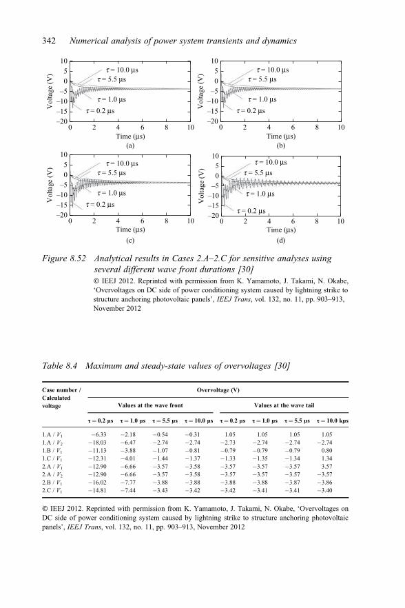
0–20–15–10

Vol

tage

(V)

–505

10

2 4Time (μs)

(a) (b)

(c) (d)

t = 0.2 μst = 1.0 μs

t = 5.5 μst = 10.0 μs

6 8 10 0–20–15–10

Vol

tage

(V)

–505

10

2 4Time (μs)

t = 0.2 μst = 1.0 μs

t = 5.5 μst = 10.0 μs

6 8 10

0–20–15–10

Vol

tage

(V)

–505

10

2 4Time (μs)

t = 0.2 μst = 1.0 μs

t = 5.5 μst = 10.0 μs

6 8 10 0–20–15–10

Vol

tage

(V)

–505

10

2 4Time (μs)

t = 0.2 μs

t = 1.0 μs

t = 5.5 μst = 10.0 μs

6 8 10

Figure 8.52 Analytical results in Cases 2.A–2.C for sensitive analyses usingseveral different wave front durations [30]� IEEJ 2012. Reprinted with permission from K. Yamamoto, J. Takami, N. Okabe,‘Overvoltages on DC side of power conditioning system caused by lightning strike tostructure anchoring photovoltaic panels’, IEEJ Trans, vol. 132, no. 11, pp. 903–913,November 2012

Table 8.4 Maximum and steady-state values of overvoltages [30]

Case number /Calculatedvoltage

Overvoltage (V)

Values at the wave front Values at the wave tail

t¼ 0.2 ms t¼ 1.0 ms t¼ 5.5 ms t¼ 10.0 ms t¼ 0.2 ms t¼ 1.0 ms t¼ 5.5 ms t¼ 10.0 kms

1.A / V1 �6.33 �2.18 �0.54 �0.31 1.05 1.05 1.05 1.051.A / V2 �18.03 �6.47 �2.74 �2.74 �2.73 �2.74 �2.74 �2.741.B / V1 �11.13 �3.88 �1.07 �0.81 �0.79 �0.79 �0.79 0.801.C / V1 �12.31 �4.01 �1.44 �1.37 �1.33 �1.35 �1.34 1.342.A / V1 �12.90 �6.66 �3.57 �3.58 �3.57 �3.57 �3.57 3.572.A / V2 �12.90 �6.66 �3.57 �3.58 �3.57 �3.57 �3.57 �3.572.B / V1 �16.02 �7.77 �3.88 �3.88 �3.88 �3.88 �3.87 �3.862.C / V1 �14.81 �7.44 �3.43 �3.42 �3.42 �3.41 �3.41 �3.40

� IEEJ 2012. Reprinted with permission from K. Yamamoto, J. Takami, N. Okabe, ‘Overvoltages onDC side of power conditioning system caused by lightning strike to structure anchoring photovoltaicpanels’, IEEJ Trans, vol. 132, no. 11, pp. 903–913, November 2012


1Wave front duration (μs)

1.B/V11.C/V12.C/V12.B/V1

2.A/V1, 2.A/V2

1.A/V2

1.C/V1

2.C/V1

2.B/V1

1.A/V2

1.A/V1

1.B/V1

2.A/V1, 2.A/V2

1.A/V1

–20

–15Ove

rvol

tage

(V)

–10

–5

0

–4

–3

–2

Ove

rvol

tage

(V)

–1

0

1

2

101Wave front duration (μs)

(a) (b)

10

Figure 8.53 Overvoltage characteristics depending on the wave front duration:(a) Values at the wave front; (b) Values at the wave tail [30]� IEEJ 2012. Reprinted with permission from K. Yamamoto, J. Takami, N. Okabe,‘Overvoltages on DC side of power conditioning system caused by lightning strike tostructure anchoring photovoltaic panels’, IEEJ Trans, vol. 132, no. 11, pp. 903–913,November 2012

0–8–4

48

12

0

Vol

tage

(V)

2 4 6 8 10Time (μs)

(a) (b)

(c) (d)

r = 1, 10 Ωm

r = 100 Ωm

r = 1,000 Ωm

0–8–4

48

12

0

Vol

tage

(V)

2 4 6 8 10Time (μs)

r = 1, 10 Ωm

r = 100 Ωm

r = 1,000 Ωm

0–8–4

48

12

0

Vol

tage

(V)

2 4 6 8 10Time (μs)

r = 1, 10 Ωm

r = 100 Ωm

r = 1,000 Ωm

0–8–4

48

12

0

Vol

tage

(V)

2 4 6 8 10Time (μs)

r = 1, 10 Ωm

r = 100 Ωm

r = 1,000 Ωm

Figure 8.54 Analytical results in Cases 1.A–1.C for sensitive analyses usingseveral different values of earth resistivity [30]� IEEJ 2012. Reprinted with permission from K. Yamamoto, J. Takami, N. Okabe,‘Overvoltages on DC side of power conditioning system caused by lightning strike tostructure anchoring photovoltaic panels’, IEEJ Trans, vol. 132, no. 11, pp. 903–913,November 2012


0–8–4

48

12

0

Vol

tage

(V)

2 4 6 8 10Time (μs)

(a) (b)

(c) (d)

r = 1, 10 Ωm

r = 100 Ωm

r = 1,000 Ωm

0–8–4

48

12

0

Vol

tage

(V)

2 4 6 8 10Time (μs)

r = 1, 10 Ωm

r = 100 Ωm

r = 1,000 Ωm

0–8–4

48

12

0

Vol

tage

(V)

2 4 6 8 10Time (μs)

r = 1, 10 Ωm

r = 100 Ωm

r = 1,000 Ωm

0–8–4

48

12

0V

olta

ge (V

)

2 4 6 8 10Time (μs)

r = 1, 10 Ωm

r = 100 Ωm

r = 1,000 Ωm

Figure 8.55 Analytical results in Cases 2.A–2.C for sensitive analyses usingseveral different values of earth resistivity [30]� IEEJ 2012. Reprinted with permission from K. Yamamoto, J. Takami, N. Okabe,‘Overvoltages on DC side of power conditioning system caused by lightning strike tostructure anchoring photovoltaic panels’, IEEJ Trans, vol. 132, no. 11, pp. 903–913,November 2012

Table 8.5 Maximum and steady-state values of overvoltages [30]

Case number /Calculatedvoltage

Overvoltage (V)

Values at the wave front Values at the wave tail

r¼ 1 Wm r¼ 10 Wm r¼ 100 Wm r¼ 1 kWm r¼ 1 Wm r¼ 10 Wm r¼ 100 Wm r¼ 1 kWm

1.A / V1 �2.86 �2.75 �2.18 �1.41 �0.09 0.02 1.05 11.391.A / V2 �7.49 �7.35 �6.47 �3.88 �3.87 �3.76 �2.74 7.581.B / V1 �5.56 �5.36 �3.88 �2.29 �1.78 �1.69 �0.79 8.231.C / V1 �6.04 �5.79 �4.01 �2.01 �2.40 �2.33 �1.35 8.862.A / V1 �7.83 �7.61 �6.66 �3.15 �4.70 �4.60 �3.57 6.732.A / V2 �7.83 �7.61 �6.66 �3.15 �4.70 �4.60 �3.57 6.732.B / V1 �8.67 �8.63 �7.77 �4.06 �4.86 �4.77 �3.88 5.112.C / V1 �8.46 �8.31 �7.44 �3.02 �4.55 �4.44 �3.41 6.78

� IEEJ 2012. Reprinted with permission from K. Yamamoto, J. Takami, N. Okabe, ‘Overvoltages onDC side of power conditioning system caused by lightning strike to structure anchoring photovoltaicpanels’, IEEJ Trans, vol. 132, no. 11, pp. 903–913, November 2012


–9

–8

–7

–6

–5

–4

–3

–2

–1

(a) (b)

1 10 100 1,000

Ove

rvol

tage

(V)

Ground resistivity (Ωm)1 10 100 1,000

Ground resistivity (Ωm)

1.A/V1

1.A/V2

1.B/V1

2.A/V1, 2.A/V22.C/V1

2.B/V1

1.C/V1

–5

0

5

10

Ove

rvol

tage

(V)

1.A/V1

1.A/V2

1.B/V1

2.A/V1, 2.A/V2

2.C/V1

2.B/V11.C/V1

Figure 8.56 Overvoltage characteristics depending on the earth resistivity:(a) Values at the wave front; (b) Values at the wave tail [30]� IEEJ 2012. Reprinted with permission from K. Yamamoto, J. Takami, N. Okabe,‘Overvoltages on DC side of power conditioning system caused by lightning strike tostructure anchoring photovoltaic panels’, IEEJ Trans, vol. 132, no. 11, pp. 903–913,November 2012

50 m

Structure

PV array

Distributionboard

CV 8 mm2–2C IV 5.5 mm2

Vinyl pipe (28)

Steel tower

IV 5.5 mm2

PCS

R = 500 ΩI.G.

Box

Figure 8.57 Experimental set-up [37]� IEEE 2013. Reprinted with permission from Sakai, K. and Yamamoto, K.,‘Lightning protection of photovoltaic power generation system: Influence ofgrounding systems on overvoltages appearing on DC wirings’, IEEE XPLORE 2013,XII SIPDA, pp. 418–422, October 2013


21.3 V, and maximum output current of 3.05 A) in series. The injection wire of thesurge current is connected with the module frame of array no. 12 through theresistance of 500 W.

The earthing resistance of the facilities is measured. A one-rod electrode isinstalled for two arrays. The installation mounts of the array are connected to eachother with insulated wires with a cross-sectional area of 2 mm2. The combinedearthing resistance of the entire array is about 14 W. The earthing resistance of theentire PV system connected with the entire array mounts, the distribution board,and the building is about 0.5 W, which is almost equal to the earthing resistance ofthe building that has low earthing resistance. In this study, it was impossible tomeasure the earthing resistance of the distribution board individually because theunderground connection wire was not able to be disconnected.

Two single-core CV cables with a cross-sectional area of 5.5 mm2 protected bymetal piping with a cross-sectional area of 22 mm2 are utilized as the wires fromthe array to the positive and negative electrodes at the distribution board. Theovervoltage between the positive and negative DC wirings of the array and theearth at the distribution board has been measured.

The experiments are conducted following two conditions. In the firstcondition, the earthing systems of the rod electrode of each array, the installation

Figure 8.58 PV arrays outline [37]� IEEE 2013. Reprinted with permission from Sakai, K. and Yamamoto, K., ‘Lightningprotection of photovoltaic power generation system: Influence of grounding systems onovervoltages appearing on DC wirings’, IEEE XPLORE 2013, XII SIPDA, pp. 418–422,October 2013


mount, and the distribution board are connected. This condition is called‘‘integrated earthing.’’ In the second condition, the earthing systems of each arrayand the rod electrode are connected, but the earthing systems of the array anddistribution board are not connected. This condition is called ‘‘independentearthing.’’

27.9°

20°

1.57 m

0.58 m

0.35 m0.05 m

Soil

1.75 m2.3 m

No.11, 12 PV modulesNo.9, 10 PV modulesto IG

Injected point

1 m

Earth electrodesFoundation Conjunction grounding wire

1.1 m

(a)

(b) (c)

(d)

Figure 8.59 Installation of PV arrays: (a) Earthing system of PV arrays;(b) Wiring layout; (c) Metal pipes under a PV array; (d) Layout ofPV modules in a PV array [37]� IEEE 2013. Reprinted with permission from Sakai, K. and Yamamoto, K., ‘Lightningprotection of photovoltaic power generation system: Influence of grounding systems onovervoltages appearing on DC wirings’, IEEE XPLORE 2013, XII SIPDA, pp. 418–422,October 2013


Figure 8.61 shows the injected current waveform, a steep-fronted wave whenthe injected current is used; its maximum current is 18.4 A at 0.35 ms.

In the case of the independent earthing, Figure 8.62 shows the overvoltages atthe array no. 12. The overvoltage at other arrays became smaller than that at no. 12,and the shape of the waveform was similar. Therefore, these waveforms are notshown in this chapter. The overvoltages between the positive and negative DCwirings of the array and the earth at the distribution board became very similarbecause the positive wire was placed close to the negative wire. In this chapter,only the overvoltage between the negative wire and the earth is shown inFigure 8.62.

At array no. 12, a larger voltage between the positive/negative wirings and theearth appeared as compared to those at other arrays. The voltage reached at 335 Vat 0.25 ms. Then, the voltage droped to 190 V and kept the constant value of about210 V until 80 ms during the measurement period. The voltage between the positiveand negative wirings became almost zero because the waveforms of the positiveand negative wirings were very similar.

FoundationEarth electrode

to I.G.PV array

Steel box

Distribution board

Metal pipe (22)

IV 5.5 mm2

Positive or negative wiring

Vinyl pipe (28)

Figure 8.60 Arrangement of wirings

–5

0

5

10

15

20

25

0 1 2 3 4 5 6 7 8

Cur

rent

(A)

Time (μs)

Figure 8.61 Injected current into the PV arrays shown in Figure 8.58


In the case of the integrated earthing, Figure 8.63 shows the overvoltage at thearray no. 12. The waveforms of the overvoltage between the negative power lineand the earth appeared in array no. 12 showed damped oscillation. The maximumovervoltage between the negative power line and the earth was 250 V at 0.2 ms, andthen the voltage between the power lines and the earth kept the constant of 9 V. Thevoltage between the positive and negative wirings became almost zero because thewaveforms of the positive and negative wirings were very similar.

8.2.2.2 Discussions of overvoltageIn the case of the independent earthing, the potential of the mounts and supportingstructures of the arrays rises when the current is injected. The potential of thedistribution board also rises depending on the potential rise around the mounts nearthe distribution board. However, both the earthing systems of the mounts and thedistribution board are not connected; the potential of the mounts and the supportingstructures is larger than that of the distribution board. The potential of the positive/negative wirings rises due to the inductive and electrostatic coupling between the

0

100

200

300

400

0 1 2 3 4 5 6 7 8

Vol

tage

(V)

Time (μs)

Figure 8.62 Overvoltage in the case of the independent earthing

0

100

200

300

400

0 1 2 3 4 5 6 7 8

Vol

tage

(V)

Time (μs)

Figure 8.63 Overvoltage in the case of the integrated earthing


support structures and the wirings. The voltages between the positive/negativewirings and the earth are regarded as the difference between the potential rise of thedistribution board and positive/negative wirings.

In the case of the integrated earthing, the earthing systems of the supportstructure and the distribution board are connected. The potential of the supportstructures rises when the current is injected. The potential of the support structureand the distribution board becomes similar because both are connected. Thepotential of the positive wiring and negative wiring rises due to the inductive andelectrostatic coupling between the support structure and the wirings. For such areason, the positive and negative wiring voltages to earth at the wave tail becamesmaller than that in case of the independent earthing.

Figure 8.64 shows the inside wirings of a PV module. Figure 8.65 shows thepicture of the PV module wirings. The area of the module is 0.51 m2. The areaencircled by wirings, which influences electromagnetic coupling, is 0.12 m2. Theinjected current spreads over the support structures, and generates magnetic fluxaround it. Due to this magnetic flux, the voltage occurs in the wirings connected tothe modules. However, the wirings between modules are usually processed at afactory. It is difficult to decrease the area encircled by this wiring.

8.2.2.3 Investigations by the FDTD simulationsThe FDTD simulation model has been made to reproduce and verify the measuredresults in the previous sections. Figure 8.66 shows the analytical space. Thedimension of the analytical space is 24.9 m � 8.275 m � 5.625 m and it is dividedinto cubic cells with a side length of 5 mm. The absorbing boundary condition isthe Liao’s second-order condition.

PV module framePV Cell

Wiring

25 mm

25 mm50 mm

1 mm

Figure 8.64 Inside wirings of a PV module [37]� IEEE 2013. Reprinted with permission from Sakai, K. and Yamamoto, K., ‘Lightningprotection of photovoltaic power generation system: Influence of grounding systems onovervoltages appearing on DC wirings’, IEEE XPLORE 2013, XII SIPDA, pp. 418–422,October 2013


The model of the PV system is installed on the earth shown in Figure 8.67. Thestratified earth structures of the resistivity are measured by the Wenner method.The current injection wire using a thin wire model is connected to the frame of thearray no. 12. The same current in measurements is injected through the 500 W. Thinwire models are also used for the power lines, structures supporting modules, andwirings in the modules. The wirings in the metal pipes are modeled as thin wires ina metal pipe model shown in Figure 8.68.

The earthing resistance values are compared at the experimental and calcula-tion set-ups. The comparisons are shown in Table 8.6. Under such analytical con-ditions, Vþ and V�, which are the voltages between positive/negative power linesand the earth of the distribution board, are calculated.

Figure 8.69 shows the injected current waveforms, and Figures 8.70 and 8.71show the comparisons of the overvoltage between the negative wiring and the earthat the distribution board in cases of the independent and integrated earthings,respectively.

In the case of the independent earthing, at array no. 12, the voltage between thenegative wiring and the earth reached at 330 V at 0.25 ms. Then, the voltage keptthe constant value about 200 V. The voltage between the positive and negativewirings became almost zero because the waveforms of the positive and negativewirings were very similar. These features are very similar with the measurements.

Figure 8.65 PV module wirings [37]� IEEE 2013. Reprinted with permission from Sakai, K. and Yamamoto, K., ‘Lightningprotection of photovoltaic power generation system: Influence of grounding systems onovervoltages appearing on DC wirings’, IEEE XPLORE 2013, XII SIPDA, pp. 418–422,October 2013


Injected point

8.275 m

24.9 m

1.3 m Distribution board(rectangular conductor)

Grounding electrode

Conjunction grounding wire

Foundation

2.375 m

0.5 m

1.45 m

I

Frame

Earth wire ofdistribution poles

(a)

(b)

Injected point

4.55 m

2.15 m

0.35 m

0.7 m0.35 m

0.4 m

Concrete (Dielectric (s = 0.005 S/m, er = 10))

Current lead wireR = 500 Ω

Thin wire model

Earth wireof thedistributionpoles

Distribution board

V+

V–

Figure 8.66 PV system model: (a) Outline; (b) Inside wiring

0.5 m

1.3 m

∞ m

190 Ωm

180.0 Ωm

50.0 Ωm

Figure 8.67 Earth resistivity at the experimental site


Table 8.6 Earthing resistance value

Experimental [W] Calculated [W]

PV array 14–30 11Earth electrode 120–300 260Distribution board 0.52 0.5PV arrays and distribution board 0.51 0.32

Flat conductor × 4

+

+

–

–

Thin wiresOutput terminal ofPV array no.11

Output terminal ofPV array no.12

Figure 8.68 Metal pipe model

–5

0

5

10

15

20

25

0 1 2 3 4 5 6

Cur

rent

(A)

Time (μs)

Figure 8.69 Injected current into the PV arrays

0

100

200

300

400

500

0 1 2 3 4 5

Vol

tage

(V)

Time (μs)

Experimental

Calculation

Figure 8.70 Comparison of overvoltage in the case of the independent earthing


In the case of the integrated earthing, the waveforms of the overvoltagebetween the negative power line and the earth appeared in array no. 12 showedinductive. The maximum overvoltage was 290 V at 0.15 ms, and then the voltagebetween the power lines and the earth kept the constant of �20 V. The voltagebetween the positive and negative wirings became almost zero because the wave-forms of the positive and negative wirings were very similar. For all the wave-forms, the calculation results agree well with the measured ones.

References

[1] Cotton I., Mcniff B., Soerenson T., Zischank W., Christiansen P., Hoppe-Kilpper M., Ramakers S. . . . Muljadi E. ‘Lightning protection for windturbines’. Proceedings of the 25th International Conference on LightningProtection; Rhodes, Greece, September 2000; pp. 848–853.

[2] IEC 61400-24: Wind Turbine Generator Systems-Part 24: Lightning Pro-tection. 2010.

[3] Ribrant J. and Bertling L.M. ‘Survey of failures in wind power systems withfocus on Swedish wind power plants during 1997–2005’. IEEE Transactionson Energy Conversion; March 2007; vol. 22, no. 1, pp. 167–173.

[4] Rachidi F., Rubinstein M., Montanya J., Bermudez J. -L., Rodriguez Sola R.,Sola G. and Korovkin N. ‘A review of current issues in lightning protectionof new-generation wind-turbine blades’. IEEE Transactions on IndustrialElectronics; June 2008; vol. 55, no. 6, pp. 2489–2496.

[5] NEDO: ‘Wind Turbine Failures and Troubles Investigating Committeeannual report’. 2006 (in Japanese).



[8] Yamamoto K., Noda T., Yokoyama S., Ametani A. ‘Experimental and ana-lytical studies of lightning overvoltages in wind turbine generator systems’.Electric Power Systems Research; March 2009; vol. 79, no. 3, pp. 436–442.

0

100

200

300

400

0 1 2 3 4 5 6

Vol

tage

(V)

Time (μs)

Experimental

Calculation

Figure 8.71 Comparison of overvoltage in the case of the integrated earthing


[9] Yee K. S., Chen J. S., Chang A. H. ‘Conformal finite-difference time-domain (FDTD) with overlapping grids’. IEEE Transactions on Antennasand Propagation; 1992; vol. 40, pp. 1068–1075.

[10] Kunz K. S., Luebbers, R. J. The Finite Difference Time Domain Method forElectromagnetics. Boca Raton, FL: CRC; 1993.

[11] Noda T., Yokoyama S. ‘Thin wire representation in finite difference timedomain surge simulation’. IEEE Transactions on Power Delivery; July 2002;vol. 17, pp. 840–847.

[12] Yamamoto K., Noda T., Yokoyama S., Ametani A. ‘An experimental studyof lightning overvoltages in wind turbine generation systems using areduced-size model’. Electrical Engineering in Japan; March 2007;vol. 158, no. 4, pp. 22–30.

[13] Yamamoto K., Yanagawa S., Sekioka S., Yokoyama S. ‘Transient groundingcharacteristics of an actual wind turbine generator system at a low resistivitysite’, IEEJ Transactions on Electrical and Electronic Engineering; January2010; vol. 5, no. 1, pp. 21–26.

[14] Yamamoto K., Yanagawa S. ‘Measurements of transient grounding char-acteristics at a wind turbine under construction’. ISWL2011: 3rd Interna-tional Symposium on Winter Lightning; June 2011; no. 3–4, pp. 97–101.

[15] Yamamoto K., Yanagawa S., Ueda T. ‘Field tests of grounding at an actualwind turbine generator system’. International Conference on LightningProtection (ICLP); Cagliari, Italy, September 2010; no. 1307.

[16] Yanagawa S., Natsuno D., Yamamoto K. ‘A measurement of transientgrounding characteristics of a wind turbine generator system and its con-siderations’. Asia-Pacific International Conference on Lightning (APL);Chengdu, Chinea, November 2011; pp. 401–404.

[17] Niihara J., Ametani A., Yamamoto K. ‘Transient grounding characteristics ata wind turbine with a counterpoise’. Asia-Pacific Symposium on Electro-magnetic Compatibility (APEMC); Singapore, May 2012.

[18] Yamamoto K., Yanagawa S., Yamabuki K., Sekioka S., Yokoyama S.‘Analytical surveys of transient and frequency dependent grounding char-acteristics of a wind turbine generator system on the basis of field tests’.IEEE Transactions on Power Delivery; October 2010; vol. 25, no. 4,pp. 3034–3043.

[19] Yamamoto K., Yanagawa S. ‘Grounding characteristics of a wind turbinemeasured immediately after its undergrounding’. Asia-Pacific Symposium onElectromagnetic Compatibility (APEMC); Singapore; May 2012.

[20] Yamamoto K., Yanagawa S., Ueda T. ‘Verifications of transient groundingimpedance measurements of a wind turbine generator system using theFDTD method’. International Symposium on Lightning Protection (SIPDA);Brazil, October 2011; pp. 255–260.

[21] Yanagawa S., Natsuno D., Yamamoto K. ‘An analytical surveys of transientgrounding characteristics of a wind turbine generator system and its con-siderations’. International Conference on Lightning Protection (ICLP);Vienna, Austria, September 2012.


[22] Yamamoto K. ‘Measurements of transient grounding characteristics of awind turbine generator system in mountainous area’. 2013 Asia-PacificInternational Conference on Lightning; June 2013; LPRE-437,pp. 431–434.

[23] Yoshikawa N., Ametani A., Yamamoto K., Yanagawa S. ‘Improvementof wind turbine grounding system using various grounding wires’. 2013Asia-Pacific Symposium on Electromagnetic Compatibility & TechnicalExhibition on EMC, RF/Microwave Measurement & Instrumentation; May2013.

[24] Yamamoto K., Sumi S., Yanagawa S. ‘Transient characteristic of an actualwind turbine grounding system’. 2013 Asia-Pacific Symposium on Electro-magnetic Compatibility & Technical Exhibition on EMC, RF/MicrowaveMeasurement & Instrumentation; May 2013.

[25] Yamamoto K., Sumi S., Yanagawa S., Natsuno D. ‘Transient groundingcharacteristic of a 600 kW class wind turbine’. 2012 CIGRE SC C4 Collo-quium in Japan; October 2012; no. III-4, pp. 79–84.

[26] Yamamoto K., Sumi S., ‘Validations of lightning protections for accidents ata wind farm’. XII SIPDA: International Symposium on Lightning Protection;October 2013; pp. 412–417.

[27] Yamamoto K., Yanagawa S. ‘Transient grounding characteristics of windturbines’. International Conference on Lightning Protection (ICLP); Vienna,Austria, September 2012; no. 74.

[28] Takahashi M., Kawasaki K., Matsunobu T. ‘Lightning surge characteristicand protection methods of photovoltaic power generation system’. IEEJTransactions on Power and Energy; October 1989; vol. 109, no. 10,pp. 443–450.

[29] Hernandez J. C., Vidal P. G., Jurado F. ‘Lightning and surge protection inphotovoltaic installations’. IEEE Transactions on Power Delivery; December2008; vol. 23, no. 4, pp. 1961–1971.

[30] Yamamoto K., Takami J., Okabe N. ‘Overvoltages on DC side of powerconditioning system caused by lightning strike to structure anchoringphotovoltaic panels’. IEEJ Trans. PE; November 2012; vol. 132, no. 11,pp. 903–913.

[31] Yamamoto K., Chikara T., Ametani A. ‘A study of transient magnetic fieldsin a nacelle of a wind turbine generator system due to lightning’. IEEJTransactions on Power and Energy; May 2009; vol. 129, no. 5, pp. 628–636.

[32] Matsuura S., Noda T., Asakawa S., Yokoyama S. ‘An experimental study ofsurge characteristics of a distribution line using a reduced-scale model’.IEEJ Transactions on Power and Energy; January 2008; vol. 128, no. 1,pp. 226–234.

[33] Kubo Y., Uno H., Nagaoka N., Baba Y., Ametani A. ‘Resonance char-acteristic of structure for PV panel and its influence on lightning surge’.Proceedings of the Twenty-Second Annual Conference of Power & EnergySociety. IEE of Japan; August 2011; session 27, no. 254, pp. 5, 6 (inJapanese).


[34] Betz H. D., Schumann U. Lightning: Principles, Instruments and Applica-tions – Review of Modern Lightning Research, ISBN: 978-1-4020-9078-3,Springer, New York, USA; 2009.

[35] Baba Y., Rakov V. A. ‘On the mechanism of attenuation of current wavespropagating along a vertical perfectly conducting wire above ground:Application to lightning’. IEEE Transactions on Electromagnetic Compat-ibility; August 2005; vol. 47, no. 3, pp. 521–532.

[36] Baba Y., Rakov V. A., ‘On the interpretation of grounding reflectionsobserved in small-scale experiments simulating lightning strikes to tower’.IEEE Transactions on Electromagnetic Compatibility; August 2005; vol. 47,no. 3, pp. 533–542.

[37] Sakai K., Yamamoto K. ‘Lightning protection of photovoltaic power genera-tion system’. XII SIPDA: International Symposium on Lightning Protection;October 2013; pp. 418–422.


Chapter 9

Surges on wind power plants andcollection systems

Y. Yasuda*

Definitions of the symbols and abbreviations used are included at the end ofthis chapter.

9.1 Introduction

Wind power generation has been considered as one of the most realistic options tosolve the confused energy problem in the global future. According to the latestreport by Global Wind Energy Council (GWEC), the global cumulative installedwind capacity has reached 300 GW, which is approximately a hundred times that ofa nuclear reactor [1].

Lightning protection systems (LPSs) for wind power generation are becominga more important public issue since installations of wind turbines (WT) have greatlyincreased worldwide. WTs are often struck by lightning because of their open-airlocations, special shapes, and very high construction heights. As well as seriousblade damage, breakdown accidents often occur in low-voltage and control circuitsin many wind power plants (WPPs).1 An earthing (grounding) system is one of themost important components required for appropriate LPSs in WTs and WPPs.According to the latest report by NEDO (New Energy and Industrial TechnologyDevelopment Organization) [2], the most frequent failures, more than 50%, in WTequipment are those occurring in low-voltage, control, communication circuits.Such frequent incidents in low-voltage circuit may cause a deterioration of theutilization rate and consequently cause increases in the cost of power generation.

Japan, in particular, suffers from frequent and heavy lightning strikes, anexample being the notorious ‘‘winter lightning’’ found in coastal areas of the Sea ofJapan [3, 4]. Indeed, many WTs in Japan have been hit by lightning, and winterlightning poses a specific threat due to its intense power and electric current whichare much higher than the world average [5–9]. Furthermore, due to its narrow

*Kansai University, Japan1The terminology ‘‘wind farm’’ may be also used in many literatures, which might suggest an idyllicimage where wind energy can be harvested from a natural resource. However, in modern technology,there exist huge groups of more than 100 turbines which are almost equivalent to a large thermal plant bythemselves. In this chapter, therefore, the author would like to use the terminology ‘‘wind power plant(WPP)’’ rather than ‘‘wind farm.’’

landmass, WPPs in Japan tend to be constructed in mountainous areas with highresistivity soil. Thus, earthing is one of the most important issues in Japan forprotecting WTs and WPPs from lightning.

It has been investigated and cleared that winter lightning may sometimeslead to burnout incidents of surge protection devices (SPDs) installed far fromthe WT that was actually struck by lightning (Figure 9.1). The phenomenon ofsurge invasion from a WT that is struck by winter lightning to the collectionsystem2 in the WPP is quite similar to the case of ‘‘back-flow surge’’, in whichthe lightning surge flows out from a high structure such as a communicationtower into a utility’s distribution line [12]. High resistivity soil often makes theSPDs at tower earthing systems operate in reverse and allows a surge current to

Ground wire

: Lightning current

Medium voltage line

TransformerArresters

Service line4

6

35 2

1

Controlcomponent

Figure 9.1 Concept of a ‘‘back-flow surge’’ from a WT [10]� 2009 The Institute of Electrical Engineers of Japan. Reproduced by permission ofThe Institute of Electrical Engineers of Japan

2Although the collection system is often confused by a distribution system, the terminology is clearlydefined by IEC 60050 International Electrotechnical Vocabulary; electrical system that collects thepower from a wind turbine generator system, and feeds it into a network step-up transformer or elec-trical loads (IEV 415-04-06) [11]. In this chapter, the author will use the terminology ‘‘collectionsystem’’ as the electrical network within a WPP whereas ‘‘distribution system’’ as that belongs to a utilityor a system operator.


flow back to the network. It is reported that the back-flow surge can sometimesburn SPDs or break down low-voltage circuits even far from the point of thelightning-strike.

This chapter analyzes incidents of burnout to SPDs resulting from winterlightning at a WPP using ARENE [13] and PSCAD/EMTDC [14]. Calculationswere performed to clarify the mechanism of how the back-flow surge propagates toother WTs from the directly struck WT. The calculations also clarified that burnoutincidents could easily occur even in a WT that had not been struck by the lightning.It also became evident that burnout incidents can be reduced when interconnectingearthing wires are installed between WTs.

9.2 Winter lightning and back-flow surge

It is well known among many researchers that Japan has a unique and somewhatrelentless environment that includes the notorious ‘‘winter lightning’’ in the coastalarea of the Sea of Japan. Winter lightning is a special lightning that typically hasupward flashes initiated by an upward leader from an earthed structure and has aduration of longer than several 10 milliseconds (ms). Therefore, the winter light-ning sometimes has a heavy electric charge of more than 300 coulombs, which isthe maximum value specified in IEC 61400-24:2010 [15]. In fact, a lot of incidentsof WT blades have been reported due to the winter lightning in the coastal area ofthe Sea of Japan during the last decades.3

The phenomenon of surge invasion from a WT that is struck by winterlightning to the collection system in a WPP is quite similar to the case of thewell-investigated phenomenon known ‘‘back-flow surge,’’ where high-resistivitysoil often makes SPDs in reverse and allows a surge current to flow back to thenetwork. It is interesting to note that the back-flow surge sometimes burns SPDs orbreaks down low-voltage circuits even on the WT or other equipment far from theWT of the lightning-strike.

Several breakdown and burnout incidents in low-voltage circuits and SPDs atWPPs are thought to be the result of the ‘‘back-flow surge.’’ In practice, many ofthe incidents not only involved the WT that had actually been struck by lightningbut also other WTs that had not been struck. The reason why WTs that had notbeen struck were nevertheless damaged has not been fully explained. The authorhas therefore concentrated on investigating surge analysis on a WPP [16, 17] andpresents in this chapter a case study of surge analysis using a WPP model withmultiple WTs connected to a power system. The introducing WPP models andanalyses can be considered as a good example for a surge analysis on WPPs,which can clarify the influence of the electrical and geometrical configuration of aWPP when lightning surge is propagated through a collection system from a WTto other WTs.

3Incidents in blades are one of the most important issues on lightning protection in WT; however, it isbeyond the scope of this book. For the detail information on the blade incidents and their counter-measures, see [8] and [9].

Surges on wind power plants and collection systems 361

9.3 Earthing system of wind turbines and wind power plants

9.3.1 Earthing system of WTsAccording to IEC 61400-24, a ‘‘Type A arrangement’’ (with vertical and/orhorizontal electrode) and ‘‘Type B arrangement’’ (with ring earth electrode) arerecommended for WT earthing. The type B arrangement is described as ‘‘this typeof arrangement comprises a ring earth electrode external to the structure in contactwith the soil for at least 80% of its total length or a foundation earth electrode.Additional vertical and horizontal earth electrodes may be used in combination withthe ring electrode. The electrode should be buried to a depth of at least 0.5 m.’’ Thisarrangement was originally defined as an earthing method for ordinary houses orbuildings in IEC 62305-3:2006 (originally IEC 61024-1-2, which was abolished andthe revised version was renumbered as the current standard). The concept of theearth electrode is to create equipotential bonding surrounding a house or a buildingto avoid values of step and touch voltages that conventionally are considereddangerous.

IEC 61400-24 states that, ‘‘For the ring earth electrode (or foundation earthelectrode), the mean radius (re) of the area enclosed by the ring earth electrode (orfoundation earth electrode) shall be not less than the value l1:

re � l1 ð9:1Þ

where l1 is represented in Figure 2 (note: in this chapter, the figure is denoted asFigure 9.2) according to LPS levels I, II, III and IV.’’

IEC 61400-24 also continues with, ‘‘When the required value of l1 is largerthan the convenient value of re, additional horizontal or vertical (or inclined)

00

10

20

30

40

50

60

70

80

90

100

500 1,000 1,500r Ωm

l 1 m

2,000 2,500 3,000

Class I

Class II

Classes III–IV

IEC 2097/05

Figure 9.2 Minimum length l1 defined in IEC 61400-24 [15]� 2010 IEC Geneva, Switzerland. www.iec.ch. IEC 61400-24 ed.1.0


electrodes shall be added with individual lengths lr (horizontal) and lv (vertical)given by the following equations:

lr ¼ l1 � re ð9:2Þand

lv ¼ l1 � reð Þ=2 ð9:3ÞThe number of electrodes shall be not less than the number of the down-

conductors, with a minimum of two.’’

9.3.2 Earthing system in WPPsIn IEC 61400-24, it is also mentioned on the earthing system in WPPs, where thefollowing statement can be seen: ‘‘Each wind turbine shall have its own earthingsystem. The earthing systems of the individual wind turbines and the high voltagesub-station shall preferably be connected with horizontal earthing conductors, toform an overall wind farm earthing system. This is particularly beneficial in casegood earthing resistance is difficult to obtain at each individual wind turbineposition.’’

IEC 61400-24 also recommends, ‘‘The earthing system of a wind farm is veryimportant for the protection of the electrical systems, because a low-resistanceearthing system reduces the potential difference between the different structures ofthe wind farm and so reduces the interference injected into the electrical links.’’However, the recommendation should be carefully noted because the collectionlines often has long distance more than several hundred meters between WTs andother equipment in a large WPP. A long distance wire/cable sometimes hasinductive impedance that may rise an apparent resistance in high-frequency rangesuch as lightning surge.

9.4 Wind power plant models for lightning surge analysis

9.4.1 WPP modelFigure 9.3 shows a WPP model made up of 10 wind power generators, identical inperformance and condition. In this model, it is assumed that

● A high-voltage transformer (6.6/66 kV) interconnects the power grid systemand an array of 10 wind power generators of the 1 MW class at 0.6 kmintervals connected by over-ground wires with bared wires.

● Although a wind power generator consists of a gearbox, a synchronous oran induction generator, rectifier, three-phase inverter, and so on, for thissimulation a stable synchronous generator is presumed for simplicity.

● Boost transformers for the generators (660 V/6.6 kV) are installed insidethe WT towers, or in their vicinity. SPDs are attached to the primary andsecondary terminals and connected to a common earth, as also shown in thedetailed diagram in Figure 9.3.


(a) W

PP m

odel

(b) W

T m

odel

600

m WT

#1W

T #2

WT

#3W

T #4

WPP

Grid

-inte

ract

ive

trans

form

er

Grid

syst

emIn

finite

bus

50 k

m

WT

#5W

T #6

WT

#7W

T #8

WT

#9W

T #1

0

Det

ail m

odel

(see

fig.

(b))B

oost

trans

form

er

600

m60

0 m

600

m60

0 m

600

m60

0 m

600

m60

0 m

600

m

400 Ω

Ligh

tnin

g 660

VW

T #1

WT

#1

SPD

s

6.6

kVB

oost

tran

sfor

mer

Earth

resi

stan

ce

164 Ω

Fig

ure

9.3

WP

Pm

odel

wit

h10

WT

s:(a

)W

PP

mod

el;

(b)

WT

mod

el

● As shown in the right-side figure in Figure 9.3, the present WT model isconnected to the earth resistance at three points, where each earth resistance issimulated as 20 or 50 W. Thus, the total value of the equipotentialized earthresistance of the WT is calculated as 6.67 or 16.6 W.

● Other details and constants used in the model are shown in Table 9.1.

In addition, since what we wished to observe in this simulation was the burnoutof SPDs at WTs that had not themselves been struck, we assumed that bladeburnout or explosive destruction and dielectric breakdown at the WT that hadactually been struck was prevented by certain measures.

9.4.2 Model for winter lightningA standard summer lightning event is generally assumed to have a crest peak of30 kA, a crest width of 2 ms, and a wave tail of 70 ms. By contrast, since winterlightning has varying crest widths and crest peaks, a standardized model has notbeen established. Therefore, the present modeling of winter lightning is based on themodel described in [11]. The parameters for crest peak and duration of wave tail aredetermined from a cumulative frequency distribution of lightning current wave shape.The assumptions concerning the lightning in the present analysis are as Table 9.2.

9.4.3 Model for surge protection device (SPD)To provide protection from surge invasion, it was assumed that SPDs were installedin both the primary (LV side; WT side) and secondary (HV side; collection system

Table 9.1 Analysis conditions for ARENE

WT (synchronous generator) model

Rating power [MVA] 1.00Direct-axis reactance Xd, Xd

0, Xd00 [p.u.] 2.00, 0.25, 0.20

Quadrature-axis reactance Xq, Xq0, Xq

00 [p.u.] 1.90, 0.50, 0.20time constants Tdo

0, Tdo00, Tqo

0, Tqo00 [s] 6.0, 0.03, 0.50, 0.06

Transformer model (boost/grid-interactive)

Connection method Y (neutral earthing)/D

Rating power [MVA] 1.0 10.0Rating voltage [V] 600/6,600 6,600/66,000Frequency [Hz] 60 60% Impedance [%] 15.7 1.57Mutual leakage inductance [mH] 18.2 18.2

Collection line model

Positive-/zero-phase resistance [W/km]* 0.00105/0.0210Positive-/zero-phase inductance [mH/km]* 0.83556/2.50067Positive-/zero-phase capacitance [nF/km]* 12.9445/6.4723Frequency-dependent characteristics Considered

*Values at 60 Hz.


side) terminals of the boost transformer near to each WT. The nominal dischargecurrent of the SPD was assumed to be 2.5 kA and its characteristic curve, starting atV1mA ¼ 8 kV, is shown in Figure 9.4.

The burnout of an SPD depends on whether the heat produced by the currentflowing through the SPD exceeds the thermal limit of the given SPD. To calculatethe total heat ESPD [kJ] produced by the SPD in the present analysis, it is necessaryto specify the simultaneous power PSPD(t) [W] derived from the SPD’s terminalvoltage VSPD(t) [V] and the current flowing ISPD(t) [A] through the SPD. Then, thetotal electric energy WSPD [Wh] can be calculated by integrating PSPD(t) from 0 tothe time T [s] when ISPD(t) converges to 0 kA. The total thermal energy produced inthe SPD ESPD [kJ] is given by unit conversion from WSPD [Wh]. This sequence isdescribed by the following equations.

PSPDðtÞ ¼ VSPDðtÞ � ISPDðtÞ ð9:4Þ

WSPD ¼Ð T

0 PSPDðtÞdt

3;600ð9:5Þ

ESPD kJ½ � ¼ 3:6 � WSPD Wh½ � ð9:6Þ

10–60

10

20

30

10–3 100

Current (ka)

Vol

tage

(kV

)

103

Figure 9.4 SPD model for surge analysis

Table 9.2 Parameters for summer and winter lightning

Summer lightning Winter lightning

Crest peak 30 kA 51 kA (the 16% value of the cumulativefrequency distribution of lightning)

Crest width 2 ms 2 msDuration of

wave tail70 ms 631 ms (the 16% value of the cumulative

frequency distribution of lightning)Polarity Positive (normally negative but

for comparison with winterlightning in this analysis)

Positive


9.4.4 Comparison analysis between ARENE and PSCAD/EMTDCIn the analysis in this section, two different digital transient simulators wereemployed: ARENE (non-real-time PC version), that was once produced by EDF(Electricite de France), and PSCAD/EMTDC by Manitoba HVDC ResearchCentre. Both of the simulators have similar algorism of Schneider-Bergeronmethod as well as the conventional EMTP/ATP. It is also possible to describe theabove-proposed model by the conventional EMTP and ATP [10].

The result by the two simulators is shown in Figure 9.5. The figures illustratethe graphs of impulse height of surges reaching at each WT. Figure 9.6 also givesclearly coincidence from the viewpoint of aspect of surge propagation calculatedby two different simulators, ARENE and EMTDC. It shows the accuracy of themodel description by ARENE and EMTDC for the lightning analysis on a WPP.

Figure 9.5 also shows an interesting tendency of the surge propagation in theWPP. It is clear that the surge from WT#1, which was struck by lightning, propa-gated to not only adjacent WT but also quite distant WTs far from lightning-strikeone. Moreover, it is recognized that the further the WT from the lightning-strike oneis, the longer the surge duration reached to the WT is. It suggests that a WT that was

(a)

Phase a

0Ener

gy a

bsor

bed

by S

PD (k

J)

Tr

WT#

1

WT#

2

WT#

3

WT#

4

WT#

5

WT#

6

WT#

7

WT#

8

WT#

9

WT#

10

1

2

3

4

5

Phase bPhase c

(b)

0

Ener

gy a

bsor

bed

by su

rge

arre

ster

(kJ)

Tr

WT#

1

WT#

2

WT#

3

WT#

4

WT#

5

WT#

6

WT#

7

WT#

8

WT#

9

WT#

10

1

2

3

4

5

Figure 9.6 Energy consumed by SPDs in each WT (Summer lightning Rg ¼ 6.77 W):(a) Case 1: Lightning on WT#1; (b) Case 2: Lightning on WT#10

(a)

#10

10

20

30Lightning strike

ARENE

EMTDC

40

#2 #3 #4 #5 #6Wind turbine number

Surg

e al

titud

e (k

V)

#7 #8 #9 #10

(b)

#10

10

20

30Lightning strike

40

#2 #3 #4 #5 #6Wind turbine number

Surg

e al

titud

e (k

V)

#7 #8 #9 #10

Figure 9.5 Comparison results of surge propagations (Rg ¼ 1.68 W): (a) Case 1:Lightning on WT#1; (b) Case 2: Lightning on WT#10


not struck by lightning directly even at farthest point from the lightning-strike onehas possibility to suffer from discharge incident due to a back-flow surge propagatingalong the collection line within the WPP. The mechanism of the back-flow surgepropagation and SPD’s incidents will be discussed in detail in the following section.

9.5 Mechanism of SPD’s burnout incidents due toback-flow surge

9.5.1 Analysis of the surge propagations in WPPIn this section, an analysis is performed to compare the energy consumption of the SPDsduring a summer and winter lightning. It is supposed that the lightning strikes eitherWT#1, which is the nearest WT to the grid, or WT#10, the furthest WT from the grid.

Figures 9.6 and 9.7 are the results of analyses done by ARENE (see section 9.4)in the cases of summer and winter lightning strikes, respectively. Each WT has anearth resistance of 6.67 W. In both figures, graphs (a) and (b) indicate the results inthe cases of lightning strikes to WT#1 and WT#10.

Comparing Figures 9.6 and 9.7, it is clear that the energy consumed by eachSPD is 10 to 30 times larger in the case by winter lightning than that by summerlightning. Since the wave tail of winter lighting is 631 ms, which is about 9 timeslonger than that of summer lightning, even more than the 1.7-times-higher crestpeak, it is likely that the energy consumed becomes significantly larger.

As also can be seen in both Figures 9.6 and 9.7, the SPD in phase b at the WTthat was actually struck consumed the largest energy. This is because the potentialdifference of phase b is the largest at the moment of the lightning strike. In contrast,at the other WTs, the SPD in phase c tends to consume the most energy. The furtherthe WT is from the WT that was struck, the more evident this tendency becomes.The reason why the energy consumed in the SPD of phase c tends to be the largestis thought to be the fact that the energy imbalance among three phases dependsupon a timing of lightning strike, i.e., phase angle of each phase conductor, at thestruck WT. When the line voltage in phase c at the moment of the lightning strike isthe highest among the three phases at the struck WT, the voltage between both

0

Ener

gy a

bsor

bed

by S

PD (k

J)

Tr

WT#

1

WT#

2

WT#

3

WT#

4

WT#

5

WT#

6

WT#

7

WT#

8

WT#

9

WT#

10

5

10

15

20

25

84 kJ123 kJ

67 kJ82 kJ

105 kJ84 kJ

Limitation of 2.5-kA SPD

(a) (b)


0

Ener

gy a

bsor

bed

by su

rge

arre

ster

(kJ)

Tr

WT#

1

WT#

2

WT#

3

WT#

4

WT#

5

WT#

6

WT#

7

WT#

8

WT#

9

WT#

10

5

10

15

20

25

Figure 9.7 Energy consumed by SPDs in each WT (Winter lightning Rg ¼ 6.77 W):(a) Case 1: Lightning on WT#1; (b) Case 2: Lightning on WT#10


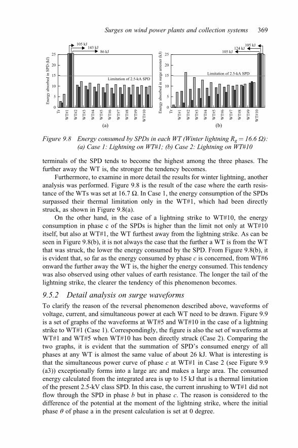
terminals of the SPD tends to become the highest among the three phases. Thefurther away the WT is, the stronger the tendency becomes.

Furthermore, to examine in more detail the results for winter lightning, anotheranalysis was performed. Figure 9.8 is the result of the case where the earth resis-tance of the WTs was set at 16.7 W. In Case 1, the energy consumption of the SPDssurpassed their thermal limitation only in the WT#1, which had been directlystruck, as shown in Figure 9.8(a).

On the other hand, in the case of a lightning strike to WT#10, the energyconsumption in phase c of the SPDs is higher than the limit not only at WT#10itself, but also at WT#1, the WT furthest away from the lightning strike. As can beseen in Figure 9.8(b), it is not always the case that the further a WT is from the WTthat was struck, the lower the energy consumed by the SPD. From Figure 9.8(b), itis evident that, so far as the energy consumed by phase c is concerned, from WT#6onward the further away the WT is, the higher the energy consumed. This tendencywas also observed using other values of earth resistance. The longer the tail of thelightning strike, the clearer the tendency of this phenomenon becomes.

9.5.2 Detail analysis on surge waveformsTo clarify the reason of the reversal phenomenon described above, waveforms ofvoltage, current, and simultaneous power at each WT need to be drawn. Figure 9.9is a set of graphs of the waveforms at WT#5 and WT#10 in the case of a lightningstrike to WT#1 (Case 1). Correspondingly, the figure is also the set of waveforms atWT#1 and WT#5 when WT#10 has been directly struck (Case 2). Comparing thetwo graphs, it is evident that the summation of SPD’s consumed energy of allphases at any WT is almost the same value of about 26 kJ. What is interesting isthat the simultaneous power curve of phase c at WT#1 in Case 2 (see Figure 9.9(a3)) exceptionally forms into a large arc and makes a large area. The consumedenergy calculated from the integrated area is up to 15 kJ that is a thermal limitationof the present 2.5-kV class SPD. In this case, the current inrushing to WT#1 did notflow through the SPD in phase b but in phase c. The reason is considered to thedifference of the potential at the moment of the lightning strike, where the initialphase q of phase a in the present calculation is set at 0 degree.

0

5

10

15

20

25Tr

WT#

1

WT#

2

WT#

3

WT#

4

WT#

5

WT#

6

WT#

7

WT#

8

WT#

9

WT#

10 Tr

WT#

1

WT#

2

WT#

3

WT#

4

WT#

5

WT#

6

WT#

7

WT#

8

WT#

9

WT#

10

0

5

10

15

20

25

105 kJ143 kJ

86 kJ105 kJ

124 kJ105 kJ

Ener

gy a

bsor

bed

in su

rge

arre

ster

(kJ)

Ener

gy a

bsor

bed

in S

PD (k

J)


(a) (b)


Figure 9.8 Energy consumed by SPDs in each WT (Winter lightning Rg ¼ 16.6 W):(a) Case 1: Lightning on WT#1; (b) Case 2: Lightning on WT#10


Thus, from the above discussion, it becomes clear that during strong winterlightning strikes with a long tail there is a possibility of SPD burnout incidents notonly at the WT that the lightning strikes and those nearby, but also at WTs far awayfrom the one that was actually struck.

As a conclusion in this section, an analysis on burnout incidents of SPDs resultingfrom winter lightning at a WPP was performed. The results of calculations clarifiedthe mechanism of how back-flow surge propagates to other WTs from the WT that hasbeen directly struck by winter lightning. The calculations with various lightning pointand earth resistance values demonstrated that burnout incidents could quite easilyoccur even in a WT far from the lightning-struck WT within the WPP. Consequently,it also became evident that the possibility of burnout incidents can become high in thecase of high resistance at the WPP site and/or long-tail winter lightning.

9.6 Effect of overhead earthing wire to prevent back-flow surge

The aim of the analysis in the present section is to clarify the influence of earthingwire(s) of the collection line in a WPP. Reference [11] also noted that earthing wire(s)

–20

–10

0

10

20

–20

–10

0

10

20

0.0

0.5

1.0

1.5

0.0

0.5

1.0

1.5

0

5

10

15

20

0

5

10

15

20

0.0 0.5 1.0 1.5 2.0

(a2)

(a1)

Phase b

Phase b

Phase aPhase c

Phase c

Phase a

(b3)

(b2)

(b1)

(a3)

Sb= 6.9 kJSa= 9.3 kJ

Sc= 10.9 kJ

Sb= 6.0 kJ

Sa= 9.6 kJ

Sc= 10.8 kJ

Sa+ Sb+ Sc= 27.1 kJ Sa+ Sb+ Sc= 25.8 kJ

Time (ms)

(a) (b)

0.0 0.5 1.0 1.5 2.0Time (ms)

Cur

rent

(kA

)V

olta

ge (k

V)

Pow

er (M

W)

Figure 9.9 Waveforms of voltage, current, and simultaneous consumption powerat SPDs in each WT (Winter lightning Rg ¼ 16.6 W, Case 1):(a) WT#5; (b) WT#10 [16]� 2008 IEEE. Reprinted, with permission, from Y. Yasuda, N. Uno, H. Kobayashi,T. Funabashi, ‘Surge analysis on wind farm when winter lightning strikes’, IEEETransactions on Energy Conversion, vol. 23, no. 1, March 2008


can reduce burnouts of SPDs in the case of a communication tower. This sectiontries to clarify if there is a similar effect from the installation of earthing wire(s) forWPP LPS. The model description and calculation has been done by PSCAD/EMTDC (see section 9.4).

The phenomenon of surge invasion to the WPP collection system from a WTthat is struck by lightning is quite similar to the back-flow surge reported in [11].In that report, the surge flowed from a communication tower into a utility’sdistribution line. High-resistivity soil often creates SPDs for tower earthing systemsto operate in reverse and allows reflux of the surge current to the distribution line. Itis reported that the back-flow surge can sometimes burn out SPDs or break downlow-voltage circuits even on an electric pole far from the point of the lightning-strike.

Several breakdown and burnout incidents in low-voltage circuits and SPDs inWPPs are thought to be the result of the above back-flow surge. In practice, manyof the incidents that have occurred not only involved the actual lightning-struckWT but also other WTs that had not been struck. The reason why WTs that had notbeen struck were nevertheless damaged has not been fully explained.

9.6.1 Model of a collection line in a WPPComparing the previous section, the simpler model for a WPP with two WTs isemployed as illustrated in Figure 9.10. The main different point of a model of acollection system is the existence of earthing wire(s) as shown in Figure 9.10(b).The collection line in the present WPP model is assumed as an overhead line withthree-phase conductors installed 10 m over the ground. Configuration details areshown in Figure 9.11 and a set of parameters is shown in Table 9.3.

The main aim of the present analysis is to confirm the effect of earthing wire(s).Various conditions, therefore, are simulated:

1. ‘‘Case 0’’: no earthing wires are installed above the overhead line.2. ‘‘Case 1’’: one earthing wire is tensioned 1 m above the three phase conductors.

Both terminals of the earthing wire are connected to the common earthingsystem of the WTs and the grid-interactive transformer.

3. ‘‘Case 2’’: two earthing wires horizontally separated at 0.7 m length above theconductors are installed.

(a) (b)

LightningBoost transformer

SPDs

Earthresistance

Collection line(WWP)

WT #1

400 ΩGrid-interactivetransformer Infinite bus

WPP Grid system

50 km

Boosttransformer

0.5 km 0.5 km

WT#2Det

ail m

odel

(see

fig.

(b))

WT#1

660 V

6.6 kV

66 kV

660 V 6.6 kV

Phase conductors

Earthing wire(s)

Wind tower

Tow

er

Figure 9.10 WPP and WT model: (a) WPP model with two WTs; (b) WT model


In the following section, comparisons will be made between the energy con-sumption of the SPDs among the three cases with various numbers of earthing wires.It is assumed that the lightning strikes WT#1, which is the nearest WT to the grid.

9.6.2 Observation of waveforms around SPDsFigure 9.12 sets out the results of EMTDC calculations in the cases of winterlightning strikes. Column (A) denotes the various waveforms measured around theSPD (phase a) installed at the high voltage terminal of the boost transformer ofWT#1. In the WT#1 SPD, since the lightning surge invades to the common earthingsystem and operates the SPD in reverse, from earth to the line, the polarity of eachwaveform was inverted. Also, Columns (B) and (C) correspond to the waveformsaround the SPD at WT#2 and the grid-interactive transformer, respectively. Thephenomena of a back-flow surge in the WPP can easily be recognized.

On the other hand, the graphs in Row (1) show voltage waveforms between theterminals of the respective SPDs. Row (2) is for current waveforms flowingthrough the SPD, and Row (3) is for simultaneous power according to (9.6), in thesame way. Every graph in Figure 9.12 has three curves due to the various condi-tions, i.e., Case 0, Case 1, and Case 2.

C4 C4 C5

C3C2C1C1 C2 C3

0.7 [m]

Tower: H-Frame-3H4Conductors: chukarGround_Wires: 1/2\\

0.7 [m]

0.7 [m]1 [m]1 [m]

10 [m]

0 [m]

Tower: H-Frame-3H4Conductors: chukarGround_Wires: 1/2\\

0 [m]

10 [m]

Mid-Span Sag:

0.5 [m] for Conductors0.5 [m] for Ground Wires

Mid-Span Sag:

0.5 [m] for Conductors0.5 [m] for Ground Wires

Ground Resistivity: 100.0 [ohm*m]Relative Ground Permeability: 1.0

Earth Return Formula: Analytical Approximation

Figure 9.11 Collection line model in WPP by PSCAD description. (Left:one-earthing-wire model, Right: two-earthing-wires model) [16]� 2008 IEEE. Reprinted, with permission, from Y. Yasuda, N. Uno, H. Kobayashi,T. Funabashi, ‘Surge analysis on wind farm when winter lightning strikes’, IEEETransactions on Energy Conversion, vol. 23, no. 1, March 2008


Comparing Case 0 and Case 1, it can be clearly seen that the effect of the earthingwire to reduce the surge reaching the next WT and the grid transformer is quite sig-nificant. From the three graphs in Row (1), it is clear that the surge durations at everypoint in the WPP are reduced by half. The surge current passing through the SPDshown in Row (2) is also cut down by almost half or two-thirds. Consequently, thesimultaneous power produced in the SPD becomes much lower, as shown in Row (3).

9.6.3 Evaluation of the possibility of the SPD’s burning outIn Row (3) of Figure 9.12, the integral area surrounding the simultaneous powercurve becomes equal to the thermal energy produced in the SPD. Summarizingthe above integration, the bar graphs shown in Figure 9.13 are drawn to evaluate the

Table 9.3 Analysis conditions for EMTDC

WT (synchronous generator) model

Rating power [MVA] 1.0Rating voltage [kV] 0.66

Impedance(R-L-C model)

Resistance [W] 0.002Inductance [mH] 0.231Capacitance [mF] 0.001

Transformer model (boost/grid-interactive)

Connection method Y/D

Rating power [MVA] 1.0 10.0Rating voltage [kV] 0.66/6.6 6.6/66Frequency [Hz] 60No load losses [p.u.] 0.0Copper losses [p.u.] 0.005Positive sequence leakage inductance [p.u.] 0.15Saturation noAircore reactance [p.u.] 0.2Magnetizing current [%] 1.0

Collection Line Model in WPP

Phase conductors Height of all conductors [m] 10Configuration of conductors HorizontalSpacing between phases [m] 0.7Conductor radius [mm2] 20.3Sag for all conductors [m] 0.5Number of sub-conductors in a bundle 1

Earthing wire Earthing wire radius [mm2] 5.5Number of earthing wire(s) 0, 1, 2Height of earthing wire(s) [m] 11Spacing between earthing wires [m] (in case of two wires) 0.7Sag for all earthing wires [m] 0.5Resistivity of earth [Wm] 100


–20 –8 0 0

500

1,00

0Ti

me

(μs)

1,50

0(A3)

(B3)

(C3)

(A2)

(B2)

Cas

e 0

(B) W

T#2

(C) T

r(A

) WT#

1

Cas

e 1

Cas

e 2

(C2)

(A1)

(B1)

(C1)

2,00

0

50

SPD power (MV)SPD current (kA)SPD voltage (kV)

100

150

020

050

01,

000

Tim

e (μ

s)1,

500

2,00

0

406080

0 050

01,

000

Tim

e (μ

s)1,

500

2,00

0

40 206080

–6–4–202

–101234

–101234

–101020 0

–20

–101020 0

–20

–101020 0

Inte

grat

ed a

rea

(con

sum

ptio

n en

ergy

)S G

W2 =

25.

0 kJ

(B1)

(C1)

(A3)

Inte

grat

ed a

rea

(con

ssum

ptio

n en

ergy

)S G

W2

WW =

25.

0 kJ

(B2)

Cas

e 0

a

Cas

e 1

Cas

e 2

Fig

ure

9.12

Cal

cula

ted

wav

efor

ms

atSP

Ds

atva

riou

spo

ints

amon

gth

eW

PP

inca

seof

win

ter

ligh

tnin

g(2

/631

ms,

51kA

)

possibility of a burnout incident at the SPDs. Column (1) in Figure 9.13 illustratesthe results of the integration area of simultaneous power curves, i.e., theenergy consumption in each SPD. The graph of WT#1, which is directly struck bylightning, displays a tendency to produce huge thermal energy in the SPDs. Thissuggests that there is a definite possibility of burnout incidents under the conditionsfound with huge winter lightning strikes. Since the total earth resistance of the WTis assumed as 3.33 W in the present case, it becomes clear that a lower resistance ora higher rate for the SPD is needed to avoid burnouts.

The most important result presented here is shown in Row (B) in Figure 9.13.From this graph of the energy consumption in the SPD of WT#2, the successful effectof installing earthing wire(s) is evident. If an earthing wire was not installed (Case 0),a huge quantity of energy could surge in, even to the adjoining WT that was notdirectly struck by the lightning. By contrast, in the case of earthing wire employment(Case 1), the surge energy invading to WT#2 is cut down to less than half. Moreover,the results for Case 2 show that the surge energy can be suppressed by much less than15 kJ, which is the thermal limitation of a 2.5-kA class SPD.

A comparison between the different numbers of earthing wires also gives aninteresting result. From the results in Figure 9.13, a multiple earthing wire strategyprovides a further margin of safety against lightning surge. As a similar tendency,to that in the present calculation for the back-flow surge, is noted in the case of acommunication tower in [11], it becomes evident that a back-flow surge in a WPPcan be reduced by the installation of earthing wire(s).

0 40 80 120 160

0 20 40 60

0 20 40 60

0 20 40 60 80

0 10 20 30 40

0 10 20 30 40

Case 0

Case 1

Case 2

Case 0

Case 1

Case 2

Case 2

Case 0

Case 1

(b)(a)

(C) T

r(A

) WT#

1(B

) WT#

2

EPR (kV)Consumption energy (kJ)

15 kJ

15 kJ

15 kJ

Thermal limitation of 2.5-kA SPD

Figure 9.13 Energy consumption at SPDs and maximum EPR at the selectedpoint in WPP in case of winter lightning (2/631 ms, 51 kA):(a) Consumption energy at SPD; (b) Maximum EPR


9.6.4 Evaluation of potential rise of earthing systemFinally, we need to also mention that a negative influence from an earthing wire(s)installation. Column (2) of Figure 9.13 shows a surprising result. The graph of an EPRat WT#2 demonstrates an upward trend according to increases in the number ofearthing wires. The same tendency can be recognized in the result in the grid-inter-active transformer (Tr). Even worse is that the additional installation of earthing wiresdoes not contribute very much to a reduction of the EPR at WT#1’s earthing system.

Another result of calculation in case of summer lightning (2/70 ms, 30 kA) isshown in Figure 9.14, where there is barely possibility of an SPD’s burnout becausethe total energy of the back-flow surge due to summer lightning is much smallerthan that of winter lightning. From Figure 9.14, it is also evident that the EPR at theequipment that are not struck by lightning tends to increase because of the instal-lation of earthing wire(s). Comparing with the case of winter lightning, the altitudeof the EPR due to summer lightning is relatively small. However, there still remainsnegative impact given by the earthing wire(s).

The reason of this negative impact seems to be because an earthing wire of0.4 km has relatively strong inductive impedance against a high frequency domainof more than 1 MHz, such as found in a lightning surge. However, since the currentflowing through the interconnecting earthing wire tends to be large, the EPR of thenext WT or a grid-transformer displays an increasing tendency. This may give riseto a possibility of breakdowns of low-voltage circuits inside the WT. While it canbe concluded that an earthing wire strategy is very effective against winter light-ning, it may cause unexpected effects in the case of summer lightning.

0 20 40 60 80 100

0 5 10 15 20

0 5 10 15 20

Case 0

Case 1

Case 2

Case 0

Case 1

Case 2

Case 0

Case 1

Case 2

(C) T

r(A

) WT#

1(B

) WT#

2

EPR (kV)

Figure 9.14 Maximum EPR at points around the WPP in case of summerlightning (2/70 ms, 30 kA)


9.7 Conclusions

In this chapter, lightning surge analyses on a WPP were performed using ARENE(section 9.5) and PSCAD/EMTDC (section 9.6). The analyses simulated a WPP usinga simple model with WTs, boost transformers, SPDs, and a gird-interactive transfor-mer connected with a collection system. From the results of several analyses the fol-lowing conclusions were obtained: (1) A back-flow surge can propagate to other WTsfrom the WT that has been directly struck by winter lightning via the earthing systemand the collection line in a WPP. (2) Burnout incidents of SPDs could quite easilyoccur even in a WT far from the lightning-struck WT. (3) Installing multiple earthingwires to the collection line in a WPP can reduce the burnout incidents due to winterlightning. (4) The earthing wire may not help, especially for summer lightning, toreduce the EPR (earth potential rise) of WTs and the grid-interactive transformer.

Consequently, the results of the present calculations suggest that an accurateearthing design and an LPS strategy must be implemented for WTs situated inWPPs. If a WPP is to be constructed in an area affected by heavy winter lightning,multiple earthing wires and higher rated SPDs should be installed to avoid burnoutsof the SPDs and other equipment. If a given WPP also potentially suffers fromsummer lightning, the installation of earthing wire(s) is not recommended becausethe interconnection of earthing wires does not have a good effect on reducing theEPR. In both cases, trials to reduce earth resistance should be selectively done forthe particular WT that would tend to suffer from lightning because of the prevailingwind direction or geographical condition.

The introduced WPP model in this chapter employed overhead earth wires inits collection lines, which is cheaper equipment than underground cables and can beseen in many existing WPPs. On the analysis on the WPPs with undergroundcables, the modeling and result of the analysis would be completely different. Asbared cables may usually be used for the interconnection between WTs in a WPP, itis slightly difficult to model the horizontal bared cables in EMTP and other similarsimulators as well as FDTD method. Here, the author would like only to suggestseveral foreseeing references [18, 19] and expect further investigations in future.

Symbols and abbreviations

ISPD (t) [A] surge current that flow through an SPD

l1 [m] minimum length defined in IEC 62035-3

lr [m] horizontal length of buried electrode

lv [m] vertical length of buried electrode

PSPD (t) [kJ] thermal energy that is produced in an SPD

R [W] resistance to earth (in this chapter, simply ‘‘earth resistance’’)

Rg [W] total earth resistance at a WT

T [s] duration during a surge current flow through an SPD

VSPD (t) [V] voltage that is imposed on an SPD

WSPD (t) [Wh] electric energy that is consumed in an SPD

r [W m] resistivity of soil


ARENE (a commercial name of a digital transient simulator)

ATP Alternative Transient Program

FDTD Finite Deference Time Domain

EMTP Electro-Magnetic Transient Program

EPR Earth Potential Rise

GWEC Global Wind Energy Council

GUI Graphical User Interface

HV high voltage

IEC International Electro-technical Commission

LPS Lightning Protection System

LV low voltage

NEDO New Energy and Development technology Organization, Japan

PSCAD/EMTDC (a commercial name of a digital transient simulator)

SPD surge protective device

WPP wind power plant

WT wind turbine

Acknowledgments

The author thanks the International Electrotechnical Commission (IEC) for per-mission to reproduce information from its International Standards IEC 61400-24ed.1.0 (2010). All such extracts are copyright of IEC, Geneva, Switzerland. Allrights reserved. Further information on the IEC is available from www.iec.ch. IEChas no responsibility for the placement and context in which the extracts andcontents are reproduced by the author, nor is IEC in any way responsible for theother content or accuracy therein.

References

[1] GWEC. ‘‘Global installed wind power capacity in 2013—Regional Dis-tribution,’’ http://www.gwec.net/wp-content/uploads/2014/04/5_17-1_global-installed-wind-power-capacity_regional-distribution.jpg

[2] New Energy and Industrial Technology Development Organization (NEDO)Final Report on New Generation Wind Power Development Project, 2015(to be issued).

[3] Yokoyama, S., Miyake, K., Suzuki, T., Kanao, S. Winter lightning on Japan SeaCoast—development of measuring system on progressing feature of lightningdischarge, IEEE Transaction on Power Delivery, vol. 5, pp. 1418–1425, 1990.

[4] Motoyama, H., Shinjo, K., Matsumoto, Y., Itamoto, N. Observation andanalysis of multiphase back flashover on the Okushishiku Test TransmissionLine caused by winter lightning, IEEE Transactions on Power Delivery,vol. 13, no. 4, pp. 1391–1398, 1998.


[5] Wada, A., Yokoyama, S., Numata, T., Hirose, T. Lightning observation onthe Nikaho-Kogen Wind Farm, Proc. of International Workshop on HighVoltage Engineering (IWHV ’04), vol. 1, pp. 51–55 (The papers of JointTechnical Meeting on Electrical Discharges, Switching and ProtectingEngineering and High Voltage Engineering, IEE Japan, ED- 04-118, SP-04-29, HV-04-59), 2004.

[6] Shindo, T., Suda, T. Lightning risk of wind turbine generator system, IEEJTransaction on Power and Energy, vol. 129, no. 10, pp. 1219–1224, 2009.

[7] Natsuno, D., Yokoyama, S., Shindo, T., Ishii, M., Shiraishi, H. Guideline forlightning protection of wind turbines in Japan, Proc. of 30th InternationalConference on Lightning Protection (ICLP2010), No. SSA-1259, 2010.

[8] Yasuda, Y., Yokoyama, S., Minowa, M., Satoh, T. Classification oflightning damage to wind turbine blades, IEEJ Trans. on Electrical andElectronic Engineering, vol. 7, no. 6, pp. 559–566, 2012.

[9] Yasuda, Y., Yokoyama, S., Ideno, M. Verification of lightning damageclassification to wind turbine blades, Proc. of 30th International Conferenceon Lightning Protection, No. 253, 2012.

[10] Okamoto, H., Sekioka, S., Ebina, Y., Yamamoto, K., Yasuda, Y., Funabashi,T., Yokoyama, S. Energy absorption of distribution line arresters due tolightning back flow current and ground potential rise for lightning hit towind turbine generator system, IEEJ Trans. on Electric and Power, vol. 129,no. 5, pp. 668–674, 2009.

[11] IEC 60050: International Electrotechnical Vocabulary.[12] Nakada, K., Wakai, T., Taniguchi, H., Kawabata, T., Yokoyama, S., Yokota,

T., Asakawa, A. Distribution arrester failures caused by lightning currentflowing from customer’s structure into distribution lines, IEEE Transactionson Power Delivery, vol. 14, no. 4, pp. 1527–1532, 1999.

[13] Devaux, O., Lemerle, P., Delsol, O., Martino, S. ARENE: A new simulatorreduces the cost of equipment tests, Proc. of 15th International Conferenceon Electricity Distribution (CIRED ’99), No. 4/p. 4, 1999, http://www.cired.net/publications/cired1999/papers/4/4_p4.pdf.

[14] Manitoba HVDC Research Centre web page: PSCAD, https://hvdc.ca/pscad/.[15] IEC 61400-24: Wind Turbine—Part 24: Lightning Protection, 2010.[16] Yasuda, Y., Funabashi, T. Analysis on back-flow surge in wind farms, Proc. of

the International Conference on Power Systems Transients (IPST ’07), 2007.[17] Yasuda, Y., Uno, N., Kobayashi, H., Funabashi, T. Surge analysis on

wind farm when winter lightning strikes, IEEE Transactions on EnergyConversion, vol. 23, no. 1, pp. 267–262, 2008.

[18] Nagao, M., Baba, Y., Nagaoka, N., Ametani, A. FDTD electromagneticanalysis of a wind turbine generator tower struck by lightning, IEEJ Trans-action of Electric and Power, vol. 129, no. 10, pp. 1181–1186, 2009.

[19] Sekioka, S., Hatziargyriou, N. Lorenzou, M. A study of grounding systemdesign of wind turbine generator considering effective length of groundingconductors (II), The papers of Joint Technical Meeting, IEE Japan, FTE-14-027, HV-14-032, 2014.


Chapter 10

Protective devices: fault locator and high-speedswitchgear

T. Funabashi*

10.1 Introduction

A time domain model of a fault locator for transmission line faults is described inthis chapter. This model uses the MODELS language in ATP-EMTP. Also, variousfault types are modeled, using a constant or nonlinear fault resistance. It has beenfound that an impedance relay type method is influenced by the fault arc non-linearity but a current diversion ratio method is not. Errors caused by currenttransformer (CT) saturation have been examined, and the influence of the CTsaturation has been found to be negligible.

In the case of transmission line faults, the power system and customer voltagesdrop instantaneously even if the customer has a nonutility generation system.Therefore, a device that separates the power system and the customer’s facilityrapidly after the voltage sag occurs has been developed. Operational characteristicsof the new device are explained by using EMTP simulations.

10.2 Fault locator

Many fault locator algorithms were developed to be operated on digital relay data[1–7]. These methods were derived from frequency domain equations and wereestablished by a phasor simulation. The algorithms were based on the assumptionthat a fault arc had a constant impedance and did not show a nonlinear effect.However, in practice, a fault arc in air is known to show nonlinearity due to itsphysical characteristic. Also an input device may cause error in the current/voltagedetection, and this results in an error on a fault locating algorithm.

To study the influence of nonlinearity on the accuracy of a digital faultlocator, a time domain simulation must be performed considering the characteristicof the fault arc and the input device. Time domain models of the protective relaywere developed by using the electromagnetic transients program EMTP [8–10].

*Professor, Nagoya University, Japan

These use a subroutine called transient analysis of control system (TACS) [11, 12]for representing the blocks of a relay simulation.

In this chapter, a time domain model of a fault locator is described using theMODELS [13, 14] language in the ATP-EMTP [11, 12]. Various fault types aremodeled considering constant and nonlinear fault resistances, and also consideringCT saturation and an input device error.

10.2.1 Fault locator algorithmDigital fault locator algorithms are divided into two categories: one that uses datafrom one terminal of a transmission line [1–4], and the other that uses data fromboth terminals [5–7]. The former is superior in the economical viewpoint because itrequires no data transfer for long distance. The latter is superior in the accuracyviewpoint of fault location, but requires a data transfer system.

This chapter deals with a one-terminal type fault locator. The reason is sim-plicity of input data and formula. The main purpose of a simulation is looking at atransition of located distance in time domain. The power systems to which the faultlocator is applied are the 66-, 77-, and 154-kV high-resistance grounded systemswidely used in Japan. The focus is on a phase-to-ground fault because this type offault occupies about 90 percent of transmission line faults. One application is fora radial circuit and another is for a double circuit as illustrated in Figure 10.1.Corresponding formulas of fault location in a frequency domain are summarizedbelow:

(a) Impedance relay type method:

d ¼Im V � I�pol

� �Im Vu � I�pol

� � ð10:1Þ

where

Vu ¼ Zs � I þX

ZmIother

dl

d

dl

d

(a) (b)

Figure 10.1 Fault location: (a) Radial circuit (impedance relay type method);(b) Double circuit (current diversion ratio method)


(b) Current diversion ratio method:

d ¼2 � Re I0m � V �

pol

� �Re I0 þ I0mð Þ � V �

pol

n o � dl ð10:2Þ

where

d: distance from location point to fault pointdl: transmission line lengthRe(A): real part of A (A: complex number)Im(A): imaginary part of AA*: conjugate of AV: faulted-phase voltage at locator terminalVu: line drop voltage per unit lengthVpol: polarized voltage, e.g., Vpol ¼ Vbcff90� in case of phase-a locatingZs: self-impedance per unit lengthZm: mutual impedance per unit lengthI: faulted-phase current at locator terminalIother: unfaulted phase current at locator terminalIpol ¼ 3 • I0 ¼ Ia þ Ib þ Ic

I0: zero sequence current of faulted lineI0m: zero sequence current of the other line

Briefly speaking, the impedance relay type method makes fault location by divid-ing the fault phase voltage by the line voltage drop per unit length [1]. The currentdiversion ratio method [4], paying attention to that a fault current is a sum ofcurrents on the faulted line and the other line, calculates the distance on theassumption that the faulted line’s voltage drop equals to the other line’s one. Thus,the latter is applicable only to a loop network.

10.2.2 Fault locator model description using MODELSThe procedure of a simulation at a time is illustrated in Figure 10.2. A time domainmodel of a fault locator is represented using the MODELS language in the ATP-EMTP. The fault locator model shown in Figure 10.2 basically consists of fivebasic parts, which are applied in sequence.

For both the impedance relay type and the current diversion ratio methods, twofault resistance values 0.1 mW and 20 W are adopted. The line length dl is 20 kmand the fault point is 5 km from the locating terminal. Parameters of the modelsystems are

Source impedance ¼ 0.19981 þ j2.0052 (W)Substation neutral current in short circuit case ¼ 200 (A)Self-impedance ¼ 0.210.79 þ j0.6571 (W/km)Mutual impedance within the circuit ¼ 0.1257 þ j0.2700 (W/km)

Protective devices: fault locator and high-speed switchgear 383

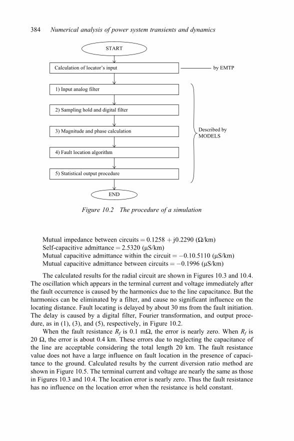
Mutual impedance between circuits ¼ 0.1258 þ j0.2290 (W/km)Self-capacitive admittance ¼ 2.5320 (mS/km)Mutual capacitive admittance within the circuit ¼�0.10.5110 (mS/km)Mutual capacitive admittance between circuits ¼�0.1996 (mS/km)

The calculated results for the radial circuit are shown in Figures 10.3 and 10.4.The oscillation which appears in the terminal current and voltage immediately afterthe fault occurrence is caused by the harmonics due to the line capacitance. But theharmonics can be eliminated by a filter, and cause no significant influence on thelocating distance. Fault locating is delayed by about 30 ms from the fault initiation.The delay is caused by a digital filter, Fourier transformation, and output proce-dure, as in (1), (3), and (5), respectively, in Figure 10.2.

When the fault resistance Rf is 0.1 mW, the error is nearly zero. When Rf is20 W, the error is about 0.4 km. These errors due to neglecting the capacitance ofthe line are acceptable considering the total length 20 km. The fault resistancevalue does not have a large influence on fault location in the presence of capaci-tance to the ground. Calculated results by the current diversion ratio method areshown in Figure 10.5. The terminal current and voltage are nearly the same as thosein Figures 10.3 and 10.4. The location error is nearly zero. Thus the fault resistancehas no influence on the location error when the resistance is held constant.

START

by EMTP

Described byMODELS

Calculation of locator’s input

1) Input analog filter

2) Sampling hold and digital filter

3) Magnitude and phase calculation

4) Fault location algorithm

5) Statistical output procedure

END

Figure 10.2 The procedure of a simulation


10.2.3 Study on influence of fault arc characteristicsHere, the case where a nonlinear arc resistance model is added to the fundamentalnetwork is examined. Many fault arc models have been proposed [15–18]. Thischapter adopts nonlinear arc resistance models and represents them by using theMODELS language.

Model-1 (square voltage method)Model-1 is a simple nonlinear resistance with the arc voltage represented as asquare wave [15, 16]:

R ¼ Va

Ij j ð10:3Þ

0–300

0.0

1.0

2.0

3.0

4.0

5.0

6.0

–200

–100

100

200

300

0

20

Current

Fault initiation

Voltage40

Time (ms)

(a)

60 80 100

0 20 40Time (ms)

Loca

tion

(km

)

Fault initiation

(b)

60 80 100

–90

90

–60

Vol

tage

(kV

)

Cur

rent

(A)

60

–30

30

0

Figure 10.3 Calculated results for the impedance relay type method: (a) Current/voltage (faulted phase); (b) Locating distance


where

R: arc resistanceI: arc currentVa: amplitude of the square wave voltage approximation (10% of phase voltage

RMS value ¼ 6.28702 kV)

Model-2 (Kizilcay’s time-dependent model)Model-2 describes the dynamic behavior of a fault through air based on measure-ment with various system voltages and types of insulation [17, 18]:

R ¼ l

gð10:4Þ

dg

dt¼ l

tðG � gÞ ð10:5Þ

G ¼ ij ju þ Rarc � ij jð Þ � len

ð10:6Þ

0–300

0.0

1.0

2.0

3.0

4.0

5.0

6.0

–200

–100

100

200

300

0

20

Current

Fault initiation

Voltage40

Time (ms)(a)

60 80 100

0 20 40Time (ms)

Loca

tion

(km

)

Fault initiation

(b)

60 80 100

–90

90

–60

Vol

tage

(kV

)

Cur

rent

(A)

60

–30

30

0



where

R: arc resistanceg: time-varying arc conductanceG: stationary arc conductancei: arc currentt: arc time constant (0.10 ms)u: constant voltage parameter per arc length (110.3 V/cm)Rarc: resistive component per arc length (0.55 mW/cm)len: time-dependent arc length (58 cm)

In this model the arc length is assumed to be constant (58 cm for the 77-kV system)because of the short arc length. Parameters t, u, and Rarc are derived from themeasurements given in [18]:

t¼ 0.10 (ms)

u ¼ 0.83�1,000/58 ¼ 110.3 (V/cm)

Rarc ¼ 32/58 ¼ 0.55 (mW/cm)

00.0

0.0

1.0

2.0

3.0

4.0

5.0

6.0

1.0

2.0

4.0

5.0

6.0

3.0

20 40Time (ms)

(a)

60 80 100

0 20 40Time (ms)

Loca

tion

(km

)

Fault initiation

(b)

60 80 100

Loca

tion

(km

)

Fault initiation

Figure 10.5 Calculated results for the current diversion ratio method: (a) Faultresistance ¼ 0.1 mW; (b) Fault resistance ¼ 20 W


In this case of steel towers, the value of the arc-voltage gradient lies between12 and 15 V/cm [19]. The value of ‘‘u’’ lies in this range.

Calculated results are shown in Figures 10.6 to 10.8. The terminal current andvoltage are nearly the same in both cases. It is clear that the impedance relay typemethod produces a large error, while the current diversion ratio method is notinfluenced by the arc resistance nonlinearity.

The effect of model parameters are investigated.

For Model-1:

Va (kV) 1, 2, 5, 10, 20, 30% of phase voltage RMS value

For Model-2:

t (ms) 0.2, 0.4, 0.6, 0.8u (V/cm) 14.3 � 10%, � 20%Rarc (mW/cm) 0.55 � 10%, � 20%len (cm) 58 þ 10%, þ 20%

0–300

0.01.02.03.04.05.06.07.08.0

–200

–100

100

200

300

0

20

Current

Fault initiation

Voltage40

Time (ms)

(a)

60 80 100

0 20 40Time (ms)

Loca

tion

(km

)

Fault initiation

(b)

60 80 100

–90

90

–60

Vol

tage

(kV

)

Cur

rent

(A)

60

–30

30

0



The calculated results are shown in Figures 10.9 and 10.10. As the location errors,produced by the current diversion ratio method, are nearly zero, the graphs ofthose results are omitted. From the figures it is observed that the locating error isproportional to the parameter values except Rarc. A highly nonlinear characteristicof the fault arc produces larger fault location errors.

10.2.4 Study on influence of errors in input devicesSimulations typically omit errors in input values introduced by measuring devicessuch as CT, CCVT, etc. For the linear characteristics of CT and CCVT, a com-pensation method described in [20] is effective. But the nonlinear (saturable)behavior of a CT is a cause of a location error, and cannot be compensated by usinga linear compensation method. Simulations were carried out considering a CT inputerror, and it was investigated how the CT’s saturable current influences the faultlocation. Many CT/CCVT models have been proposed and the influence of theirerrors on protective relays or the compensation method have been studied [21–23].In this chapter, two types of CT saturation have been simulated, one with hysteresis

0–300

0.0

1.0

2.0

3.0

4.0

5.0

6.0

7.0

8.0

–200

–100

100

200

300

0

20

Current

Fault initiation

Voltage40

Time (ms)

(a)

60 80 100

0 20 40Time (ms)

Loca

tion

(km

)

Fault initiation

(b)

60 80 100

–90

90

–60

Vol

tage

(kV

)

Cur

rent

(A)

60

–30

30

0



00.0

0.0

1.0

2.0

3.0

4.0

5.0

6.0

1.0

2.0

4.0

5.0

6.0

3.0

20 40Time (ms)

(a)

60 80 100

0 20 40Time (ms)

Loca

tion

(km

)

Fault initiation

(b)

60 80 100

Loca

tion

(km

)

Fault initiation

Figure 10.8 Calculated results for the current diversion ratio method: (a) Arcresistance model-1; (b) Arc resistance model-2

00.6287

1.2574

3.143516.28702

18.86

0

1

2

3

4

5

6

7

5 10Va (kV)

Max

imum

loca

tion

erro

r (km

)

15 20

12.57405

Figure 10.9 Sensitivity analysis of Model-1 parameters for the impedance relaytype method


00

0.5

Max

imum

loca

tion

erro

r (km

)1

1.5

2

2.5

0.2

0.2

0.4

0.4

Tau (ms)(a)

0.6 0.8

0.8

1

0.6

100

0.5

Max

imum

loca

tion

erro

r (km

)

1

1.5

2

2.5

12

12.87

u (V/cm)(b)

14 16

17.16

18

14.3

0.40

0.5

Max

imum

loca

tion

erro

r (km

)

1

1.5

2

2.5

0.45 0.5Rarc (mohm/cm)

(c)

(d)

0.55 0.6 0.70.65

0.44 0.495

560

0.5

Max

imum

loca

tion

erro

r (km

)

1

1.5

2

2.5

58 6260len (cm)

64 66 7068

11.44

15.73

69.663.858

0.660.55 0.605

Figure 10.10 Sensitivity analysis of Model-2 parameters for the impedancerelay type method: (a) Time constant t is varied; (b) u;(c) Rarc; (d) Arc length


(ATP type-96) [12] and the other without hysteresis (type-93). The CT model hasbeen used in Figure 10.11 and its saturation characteristic in Figure 10.12.

A phase-to-phase fault is located using the impedance relay type method, andresults are given in Figures 10.13 and 10.14. These results show no significantlocating errors, because most of the current measurement errors caused by the CTsaturation disappear by the time when the locator determines the fault distance. Thetime constant of the circuit is about 8.4 ms. This means that the CT saturation errordoes not influence the correctness of the fault location. Although the operation ofprotection relays is greatly affected by CT saturation, its influence can be ignoredin the application of digital fault location.

R2

R1: resistance of primary windingR2: resistance of secondary windingRb: resistance of burdeni1: primary current referred to the secondary sidei2: secondary currentie: exciting current

R1

Rb

i2

ie

TYPE 93or TYPE 96

TYPE 60

i1

Figure 10.11 CT model

–0.78

f (VS)

0.709–0.709 –0.75

0.750.78

ie (A)

TYPE 96

–0.165 1.151–1.151

0.709

0.709

TYPE 93

0.165 1.000–1.000

Figure 10.12 Saturation characteristics of CT


10.3 High-speed switchgear

A parallel operation of utility power system and nonutility generation system hasbeen increasing. For example, many combined heat and power (CHP) systems areoperated at huge industrial plants of factories. CHP will be increased not only atindustrial plants but also at nonindustry facilities such as hospitals and hotels inaspect of effective use of electrical and heat energy. However, in the case oftransmission line faults, the power system and customer voltages drop instanta-neously even if the customer has the CHP generating system. This voltage sagaffects customer’s various devices. Especially, equipment with electronic anddigital circuits is affected by the voltage sag, even if the duration of voltage sag isshort such as 0.1 second. Even when a circuit breaker operates in 0.2 second andseparates the system, load equipment with electronic and digital circuits can bedamaged easily. Therefore, a device that would separate customer’s facilities fromthe power system rapidly is required for some load equipment [24].

00.01.02.0

Loca

tion

(km

)

3.04.05.06.07.08.09.0

10.0

20

Fault initiation

40Time (ms)

(b)

Time (ms)–60

60

–40

40

–20Cur

rent

(A) 20

02020 4040 808020 40 60 80

(a)

60 80 100

Fault initiation

iei1i2

0 100

Figure 10.13 Calculated results for the impedance relay type method with CTmodel (without hysteresis): (a) CT circuit’s currents (b-phase);(b) Locating distance


In this background, a high-speed switchgear that could separate a powersystem and a CHP by using thyristors were developed [25] in purpose of protectingmost important loads from the voltage sag.

At first, the influence of the voltage sag and then the principle of the device(high-speed switchgear) are explained in this section. Second, the test results at afactory are presented and compared with simulation results by EMTP. The influ-ence of the voltage sag magnitude is studied. Finally, waveforms recorded by thedevice in the real field is presented.

Examples of the influence of the voltage sag on loads are shown in reference[24]. Most devices are affected by the voltage sag, even if the time duration iswithin 0.1 second. It can be said that they are insufficient in an aspect of ridethrough capability to the voltage sag.

A high-speed switchgear was developed in 1993 [26]. The device consists of athyristor switch, disconnecting switches, and the control circuit to detect voltagesag and synchronizing switches. The device is installed in series with the circuitbreaker, which is interconnecting the bus of the customer’s own power generation

00.01.02.0

Loca

tion

(km

)

3.04.05.06.07.08.09.0

10.0

20

Fault initiation

40Time (ms)

(b)

Time (ms)

–60

–80

60

80

–40

40

–20Cur

rent

(A) 20

020 40 60 80

(a)

60 80 100

ie

i2

0 100

i1

Fault initiation

Figure 10.14 Calculated results for the impedance relay type method with CTmodel (with hysteresis): (a) CT circuit’s currents (b-phase);(b) Locating distance


system and that supplied from a utility. It executes high-speed tripping, within onecycle of commercial frequency, when the voltage on the customer’s bus drops.

10.3.1 Modeling methodsA test circuit is illustrated in Figure 10.15. A utility power system and a CHP areconnected via a circuit breaker and a high-speed switchgear in series. The capacityof the critical load is set to be 75 percent of the generator-rated power. Instanta-neous voltage sag is generated by short circuit in the utility power system side. Thetest is simulated under two conditions to compare the performance of a conven-tional circuit breaker with that of the high-speed switchgear.

Case-1: The high-speed switchgear is short-circuited by switch-B. The gen-erator voltage, the network voltage, and the short circuit current are measured whenthe generator and the network are separated by the circuit breaker.

Case-2: Switch-B is opened. Performance of the high-speed switchgear and thepower system is measured when the device works. The voltage drop detection levelof the device is set to be 15 percent of the rated voltage.

Test and simulation results are given in Table 10.1 and the waveforms areshown in Figure 10.16.

10.3.2 Comparative study with measurementIn Case-1 of Figure 10.16(a), the circuit breaker separates the power system after300 ms. The generator voltage drop (62 percent) is too large.

Case-2 of Figure 10.16(a) shows a waveform when the high-speed switchgearis operated 15 ms after the fault occurrence, and separates the power system fromthe CHP system. When the instantaneous voltage sag occurs, the generator voltage

200 V50 Hz

Electric network Nonutility generation system

(CGS)

135 kVA200 V0.8 PF

Generator’sswitch

Generator’s voltagemeasurement point

80 kW

Critical loads

Water resistance

Switch B

(Conventional)

resistance

Switch Afor fault

Network voltagemeasurement point

Connectionswitch

Distribution line0.125 Ω

In-yard

G

Circuit breakerHigh-speed switchgear

R

Short-circuitcurrent

G

Figure 10.15 A test circuit


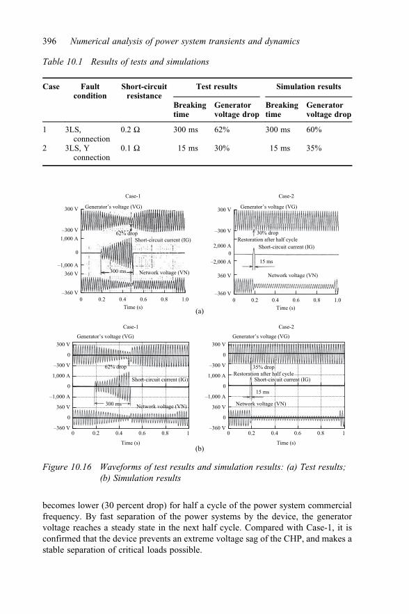
becomes lower (30 percent drop) for half a cycle of the power system commercialfrequency. By fast separation of the power systems by the device, the generatorvoltage reaches a steady state in the next half cycle. Compared with Case-1, it isconfirmed that the device prevents an extreme voltage sag of the CHP, and makes astable separation of critical loads possible.

0–360 V

–300 V

300 V

360 V–1,000 A

300 ms Network voltage (VN)

Short-circuit current (IG)62% drop

Generator’s voltage (VG)

1,000 A

0

0.2 0.4 0.6Time (s)

0.8 1.0

(b)

(a)

Case-1 Case-2

Case-1 Case-2

0–360 V

–300 V

300 V

0

360 V

–1,000 A300 ms Network voltage (VN)

Short-circuit current (IG)

62% drop


1,000 A

0

0

0.2 0.4 0.6

Time (s)

0.8 1

0–360 V

–300 V

300 V

360 V

–2,000 A

2,000 A

15 ms

Network voltage (VN)


30% dropRestoration after half cycle


0

0.2 0.4 0.6Time (s)

0.8 1.0

0–360 V

–300 V

300 V

0

360 V

–1,000 A15 ms


1,000 A

0

0

0.2 0.4 0.6

Time (s)

0.8 1

35% dropRestoration after half cycle


Network voltage (VN)

Figure 10.16 Waveforms of test results and simulation results: (a) Test results;(b) Simulation results

Table 10.1 Results of tests and simulations

Case Faultcondition

Short-circuitresistance

Test results Simulation results

Breakingtime

Generatorvoltage drop

Breakingtime

Generatorvoltage drop

1 3LS,connection

0.2 W 300 ms 62% 300 ms 60%

2 3LS, Yconnection

0.1 W 15 ms 30% 15 ms 35%


In the simulation using EMTP, the circuit breaker and the high-speed switch-gear are represented by an ordinary switch model, and a generator is represented byPark’s model [11]. Opening time of the switch is determined as the same value asthe test results. The generator voltage drop and the waveforms show a goodagreement with the test results. Thus, the validity of an EMTP simulation for thedevice has been confirmed.

10.3.3 Influence of voltage sag magnitudeIt was observed that most devices are affected by the voltage sag within 0.1 second.It has been said that the number of instantaneous voltage sags within 0.2 second ismore than 80 percent of the total voltage sags. The instantaneous voltage sagswhose magnitude is less than 20 percent occupy about 55 percent of the totalvoltage sags, and those less than 50 percent occupy about 80 percent. Taking thevalues into considerations, it can be said that a power-consuming device is notcapable of withstanding the instantaneous voltage sag.

Consumption of critical loads and general loads is set to be of 75 percent and100 percent of the generator-rated power, respectively. In Figure 10.17, a powersystem and a CHP are interconnected with each other through a circuit breaker andthe device. In the simulation it is assumed that each device is under individualoperation without information exchange. This is to study the influence of theinterrupting time of each device. Occurrence time of an instantaneous voltage sag isabout 20 ms after the simulation starts. The interrupting time of the circuit breakeris 0.2 second after the occurrence of the voltage sag. The interrupting time of thedevice is within 6.5 to 20 ms. This time is affected by the condition of the voltagesag and the phase angle of the current interruption. In this simulation the time is setto 20 ms, which is the worst case scenario. The circuit breaker and the device arerepresented by an ordinary switch model in EMTP. The generator is simulated by

77 kV50 Hz

Fault point

Tr15%Z (20 MVA)

High-speed switchgear

CGS6.0 MVA

6.6 kV0.8 PF

4.8 MW3.6 MVar

G

Circuit breaker

(Conventional)4.8 MW3.6 MVar

In yard

General load(100%)

Critical load(75%)

Generator’s voltageoutput point

3.6 MW2.7 MVar

Electricnetwork

Figure 10.17 Simulation circuit


Park’s model. The generator control circuit is simulated using TACS function ofEMTP [11]. The magnitude of the voltage sag is set to 20 and 50 percent bychanging the fault point impedance.

For the conditions of the instantaneous voltage sag of 20 and 50 percent,simulations were performed with the circuit breaker connecting buses and thedevice. Figure 10.18 shows the generator voltage simulated and the influence of theinstantaneous voltage sag for various loads mentioned above. For each condition,maximum voltage sag in the faulted period and the voltage rise are given in

0.010

0.2

0.4

0.6

0.8

1

1.2

1.4

0.1Time (s)

(b)

Voltage (pu)

Voltage (pu)

1 10

0.010

0.2

0.4

0.6

0.8

1

1.2

1.4

0.1Time (s)

(a)

1 10

:Circuit breaker

:High-speed switchgear

:Circuit breaker

:High-speed switchgear

Word processorPersonal computer

VVVF High-intensity discharge lamp

Undervoltage relay

Electromedical apparatusElectromagneticswitch

Voltage dropoccurrence

Undervoltage relay

Electromedical apparatusElectromagneticswitch

Personal computerWord processor

High-intensity discharge lampVVVF

Voltage dropoccurrence

Figure 10.18 Simulation results: (a) Voltage sag: 20% (target value);(b) Voltage sag: 50% (target value)


Table 10.2. In the simulated waveform of Figure 10.18, the voltage amplitude isoscillating by the influence of a transient direct current component during thesubtransient period (Td

00 ¼ 35 ms).When the system is interrupted by the circuit breaker under the condition of the

voltage sag of 20 percent, a high intensity discharge lamp is influenced by thevoltage sag. If interrupted by the device, it is not affected. Under the condition ofthe voltage sag of 50 percent, most load devices are influenced by the voltage sag.As the voltage rise after the interruption is greater than 20 percent, there is a pos-sibility that an overvoltage protective relay operates depending on the time delaysetting. In the case of interruption by the device, load equipment is not affected bythe instantaneous voltage sag, and the voltage rise after interruption is lower.

A voltage sag waveform is shown in Figure 10.19. It was observed in August,1995, by the device installed in a customer site with 3.3 kV rated voltage. Thedevice breaks the short circuit current at 15 ms after the instantaneous voltage saggenerated. This breaking makes the power system separated from the customer’sfacility at high speed so that the generator can continue to operate steadily and

0–1.7 kA

–6.0 kV

–6.0 kV

6.0 kV

0

6.0 kV

0

1.7 kA

0

0.025 0.05 0.075 0.1 0.125Time (s)

15 ms Current of interconnecting line

Restoration after half cycle

30% dropSteady state

Network voltage

Generator’s voltage

Instantaneous voltage drop generation

0.15 0.175 0.2

Figure 10.19 A recorded instantaneous voltage sag

Table 10.2 Maximum voltage drop during the fault and voltage rise after clearingthe fault

Voltage drop(target value)

High-speed switchgear Circuit breaker

Max. voltagedrop

Voltage riseafter breaking

Max. voltagedrop

Voltage rise afterbreaking

20% 12.0% 7.5% 23.5% 14.1%50% 32.2% 9.8% 50.9% 26.8%


restrain the voltage sag (approximately 30 percent) of the important loads withinhalf a cycle of the commercial frequency. However, the network voltage cannotrecover even when 0.1 ms or longer time is passed. No trouble was observed in thecritical loads when the high-speed switchgear was adopted.

10.4 Conclusions

This chapter has investigated the influence of the fault arc nonlinearity and theinput device error on the accuracy of digital fault locators. A time domain simu-lation model of the digital fault locator was represented using the MODELS lan-guage in the ATP-EMTP. Various types of faults were simulated with constant andnonlinear fault arc resistances. The simulation results have shown that the impe-dance relay type method is influenced by the nonlinear characteristics of the faultarc, while the current diversion ratio method is not. A sensitivity analysis of thelocating error with respect to the model parameters of the nonlinear arc resistancewas performed for the impedance relay type method. It has been observed thatthe greater the degree of nonlinearity, the greater the location error. CT errors wereconsidered, and it was observed that the CT saturation error does not last longenough to affect the fault location result and thus can be ignored.

In order to verify the operation characteristic of the high-speed switchgear, thischapter has investigated the influence of the instantaneous voltage sag and theprinciple of the device. The following remarks are obtained from the aboveinvestigation.

1. Load facilities are affected by the instantaneous voltage sag.2. Adopting thyristor switches and the scheme that can sense the instantaneous

voltage sag, this device can separate a CHP from a power system.3. A comparison of measured results with simulated results shows that the ability

of the device can be verified through the EMTP simulation.4. Test and simulation results show that most critical (sensitive) device could be

affected in the case of the circuit breaker operation. As a countermeasureagainst the instantaneous voltage sag, the device can protect most critical loadsand is running well in the field.

References

[1] Takagi, T., Yamakoshi, Y., Yamaura, M., Kondou, R., Matsushima, T.‘Development of a new type fault locator using the one-terminal voltageand current data’. IEEE Transaction on Power Apparatus and Systems,vol. PAS-101, no. 8, August 1982, pp. 2892–2898.

[2] Eriksson, L., Saha, M. M., Rockfeller, G. D. ‘An acculate locator withcompensation for apparent reactance in the fault resistance resulting fromremote-end infeed’. IEEE Transaction on Power Apparatus and Systems,vol. PAS-104, no. 2, February 1985, pp. 424–436.


[3] Sachdev, M., Agarwl, R. ‘A technique for estimating transmission line faultlocations from digital impedance relay measurements’. IEEE Transactionson Power Delivery, vol. 3, no. 1, January 1988, pp. 121–129.

[4] Suzuki, K., Ohura, Y., Kurosawa, Y., Takemura, T., Kumano, S., Yoshikawa,M., Funabashi, T., Iwatani, F. ‘Existing condition and experiences of distancerelays and fault locators using digital technology’. CIGRE SymposiumBoumemouth S34-89, 1989.

[5] Girgis, A. A., Fallon, C. M. ‘Fault location techniques for radial and looptransmission systems using digital fault recorded data’. IEEE Transactionson Power Delivery, vol. 7, no. 4, October 1992, pp. 1936–1945.

[6] Johns, A. T., Moore, P. J., Whittard, R. ‘New technique for the accuratelocation of earth faults on transmission systems’. IEE Proc.-Gener. Transm.Distrib., vol. 142, no. 2, March 1995, pp. 119–127.

[7] Novosel, D., Hart, D. G., Udren, E., Saha, M. M. ‘Fault location using digitalrelay data’. IEEE Computer Applications in Power, July 1995, pp. 45–50.

[8] Peterson, J. N., Wall, R. W. ‘Interactive relay controlled power systemmodelling’. IEEE Transactions on Power Delivery, vol. 6, no. 1, January1991, pp. 96–102.

[9] Wilson, R. E., Nordstrom, J. M. ‘EMTP transient modeling of a distancerelay and a comparison with EMTP laboratory testing’. IEEE Transactionson Power Delivery, vol. 8, no. 3, July 1993, pp. 984–992.

[10] Chaudhary, A. K. S., Tam, K., Phadke, A. G. ‘Protection system repre-sentation in the electromagnetic transients program’. IEEE Transactions onPower Delivery, vol. 9, no. 2, April 1994, pp. 700–711.

[11] Dommel, H. W. EMTP theory book. Bonneville Power Administration,1986.

[12] Scott-Meyer, W. ATP rule book. Bonneville Power Administration, 1993.[13] Dube, L., Bonfani, I. ‘MODELS: A new simulation tool in the EMTP’.

European Transactions on Electrical Power Engineering (ETEP), vol. 2,no. 1, January/February 1992, pp. 45–50.

[14] Dube, L. User’s guide to MODELS in ATP. Bonneville Power Adminis-tration, 1996.

[15] Djuric, M. B., Terzija, V. V. ‘A new approach to the arcing faults detectionfor fast autoreclosure in transmission systems’. IEEE Transactions on PowerDelivery, vol. 10, no. 4, October 1995, pp. 1793–1798.

[16] Sousa, J., Santos, D., Correia de Barros, M. T. ‘Fault arc modeling inEMTP’. IPST’95-International Conference on Power Systems Transients,Lisbon, 3–7 September 1995, pp. 475–480.

[17] Kizilcay, M., Pniok, T. ‘Digital simulation of fault arcs in power systems’.European Transactions on Electrical Power Engineering (ETEP), vol. 1, no. 1,January/February 1991, pp. 55–60.

[18] Kizilcay, M., Koch, K. H. ‘Numerical fault arc simulation based on powerarc tests’. European Transactions on Electrical Power Engineering (ETEP),vol. 4, no. 3, May/June 1994, pp. 177–185.


[19] Cornick, K. J., Ko, Y. M., Pek, B. ‘Power system transients caused by arcingfaults’. IEE Proc., vol. 128, pt. C, no. 1, January 1981, pp. 18–27.

[20] Harada, E., Yashiro, M., Mizutori, T., Funabashi, T. ‘Error compensationscheme for analog detector’. Japanese patent #1708068, November 11,1992.

[21] Working Group of the Relay Input Sources Subcommittee of the PowerSystem Relay Committee. ‘Transient response of current transformers’.IEEE Transactions on Power Apparatus and Systems, vol. PAS-96, no. 6,November/December 1977, pp. 1809–1814.

[22] Transient Response of CCVTs Working Group of the Relay Input SourcesSubcommittee of the Power System Relay Committee. ‘Transient responseof coupling capacitor voltage transformers IEEE committee report’. IEEETransactions on Power Apparatus and Systems, vol. PAS-100, no. 12,December 1981, pp. 4811–4814.

[23] Horowitz, S. H., Phadke, A. G. Power system relaying. 2nd Edition, ResearchStudies Press, Taunton, Somerset, England, 1992, pp. 59–61, 70–76.

[24] Electric Technology Research Association Report Instantaneous VoltageSag. Committee Report, 1990, vol. 46, no. 3.

[25] Matsushita, K., Matsuura, Y., Funabashi, T., Takeuchi, N., Kai, T., Oobe, M.‘Study for the performance of high speed switchgear for protection of in-house generation system’. IEEE Industry and Application Society I&CPS’96(Industrial and Commercial Power Systems Technical Conference), May 6–9,1996, New Orleans, Louisiana, USA, pp. 91–95.

[26] Matsushita, K., Kataoka, Y., Ono, M. ‘High speed switch gear for protectionof generator’. Proceeding of the Fourth Annual Conference of Power andEnergy Society, IEE of Japan (Regular Session II, Short Papers), July 28–30,1993, Hokkaido University, Sapporo, Japan, pp. 484–485.


Chapter 11

Overvoltage protection and insulationcoordination

T. Ohno*

This chapter discusses the overvoltage protection and the insulation coordinationwith a focus on the transient analysis required. The first section gives definitions oftemporary overvoltages, slow-front overvoltages, fast-front overvoltages, and very-fast-front overvoltages. The section also explains causes and characteristics of eachovervoltage. It is necessary to understand them in order to perform the insulationcoordination study.

The next section introduces the insulation coordination study based on the IEC60071 series. According to the study procedure defined in these internationalstandards, representative overvoltages first need to be determined for temporary,slow-front, and fast-front overvoltages. The determination of representative over-voltages requires extensive transient analyses, and it is the crucial part in theinsulation coordination study.

The application of surge arresters is indispensable for the overvoltage protection.The selection of surge arresters is introduced in section 11.3, according to the IEC60099 series. Specifications of surge arresters and their selection procedure areexplained. Finally, an example of the transient analysis for the overvoltage protectionand the insulation coordination is introduced in section 11.4.

11.1 Classification of overvoltages

Overvoltages are characterized by their origins, voltage shapes, and durations.Besides continuous (power-frequency) voltages, IEC 60071-1 classifies over-voltages into four categories—temporary overvoltages, slow-front overvoltages,fast-front overvoltages, and very-fast-front overvoltages [1]. Voltage shapes ofthese overvoltages are defined as in Table 11.1. This section explains these fourcategories of overvoltages in relation to the overvoltage protection and the insula-tion coordination.

*Manager, Power System Analysis Group, Tokyo Electric Power Co., Japan

11.1.1 Temporary overvoltageVoltage levels of temporary overvoltages are normally lowest among four cate-gories of overvoltages, but durations are normally longest. The long duration iscaused by low-frequency components contained in temporary overvoltages, and thelow frequency also leads to wider or deeper propagation of temporary overvoltages.

Difficulties can arise when performing the transient analysis of temporaryovervoltages since it requires the modeling of a wider area of the power system (bigmodel) [2]. Determining the extent of the modeled area is not a trivial question. Anadaption of model reduction technique is also considered.

One can encounter other difficulties due to the fact that severe temporaryovervoltages are often caused under specific network conditions [3, 4]. Finding thespecific network condition can require a number of simulation runs with a big model.

Since the severe temporary overvoltage occurs only under specific networkconditions, the probability of its occurrence is significantly low compared withother overvoltages. If such a condition exists, however, the consequence of thesevere temporary overvoltage should not be ignored. Hence, the temporary over-voltage analysis is generally conducted with the deterministic method.

Temporary overvoltages are generally caused by the following phenomena:

● Single-line-to-ground fault● Resonance● Load rejection/system islanding

When a single-line-to-ground fault occurs, the voltages of healthy phases riseuntil the fault is cleared. IEEE Std. 142 defines the effectively grounded system as asystem ‘‘grounded through a sufficiently low impedance such that for all systemconditions the ratio of zero-sequence reactance to positive sequence reactance (X0/X1)is positive and not greater than 3, and the ratio of zero-sequence resistance to positive-sequence reactance (R0/X1) is positive and not greater than 1’’ [5]. In such a system,the voltages of healthy phases are normally limited to 80% of the line voltage.

The transient analysis to find the overvoltage in healthy phases is sometimesperformed when a studied system is not effectively grounded. The overvoltage canalso be checked when the ground fault overvoltage analysis is conducted to studyslow-front overvoltages.

Table 11.1 Voltage shapes of overvoltages

Temporary Slow-front Fast-front Very-fast-front

Frequency 10–500 Hz – – 0.3–100 MHz30–300 kHz *1

Duration 0.02–3,600 s – – –Time to peak – 20–5,000 ms 0.1–20 ms �0.1 msTime to half value – �20 ms �300 ms –

*1: The very-fast-front overvoltage is superimposed on the base overvoltage. The frequency of the very-fast-front overvoltage is 0.3–100 MHz, while the frequency of the base overvoltage is 30–300 kHz.


The resonance includes the series resonance, the parallel resonance, the open-phase resonance, and the ferroresonance. The transient analysis on the series,parallel and the open-phase resonance, in other words, linear resonance, is performedin all phases—feasibility study, implementation study, and forensic analysis—of theovervoltage protection design and the insulation coordination study [2–4]. The over-voltage caused by the ferroresonance, in other words, nonlinear resonance, is oftendifficult to predict. The transient analysis on the ferroresonance is normally conductedin the forensic analysis.

Extremely severe resonance conditions can be found in the resonance over-voltage analysis. Especially, the black-start restoration can present a major difficultydue to the low load condition. Depending on the severity of the resonance, it may notbe realistic to suppress the overvoltage only by surge arresters. In such a case, theovervoltage should be avoided by operational countermeasures or other equipmentsuch as shunt reactors.

Load rejection and system islanding can cause an oscillatory overvoltage com-posed of two-frequency components, one of which is always the nominal frequencycomponent [2–4]. The superimposition of two-frequency components leads to apeculiar overvoltage waveform as shown in Figure 11.1. The overvoltage caused by theload rejection or the system islanding is suppressed by carefully selecting the com-pensation rate of the transmission line charging capacity or applying surge arresters.

11.1.2 Slow-front overvoltageMajor causes of slow-front overvoltages are the following phenomena or switchingoperations:

● Line energization and reenergization● Ground fault and fault clearing● Interruption of inductive and capacitive currents

–600

–400

–200

0

200

400

600

800

0 0.05 0.1 0.15 0.2 0.25 0.3 0.35 0.4Time (s)

Vol

tage

(kV

)phase aphase bphase c

Figure 11.1 Example of the overvoltage caused by the load rejection

Overvoltage protection and insulation coordination 405

One of the characteristics of the slow-front overvoltage analysis is the statis-tical evaluation of obtained overvoltages. The statistical method is applied to runrepeated simulations, typically a couple of hundred times, in order to consider therandomness involved in the phenomena or the switching operations.

For example, in case of the line energization overvoltage, the point-on-wavewhen each phase of the circuit breaker is closed is a random process. Generally, therandomness of the timing when the closing command is received by the circuitbreaker is modeled with the uniform distribution, and the randomness of the dif-ference of the timing between each phase is modeled with the normal distribution.

The line energization overvoltage is generally more severe than the ground faultand fault clearing overvoltage. It is studied by CIGRE Working Groups 13.02 and13.05 with different conditions such as the line length and the feeding network [6–9].

When a surge arrester is installed, however, the line energization overvoltageanalysis is often not performed as the overvoltage is suppressed by the surgearrester. The same applies to the ground fault and fault current overvoltage analy-sis. The phase-to-earth overvoltage is limited to the protective level of the surgearrester, and the phase-to-phase overvoltage is limited to twice the protective levelof the surge arrester. In many cases, the maximum phase-to-phase overvoltage ismuch lower than this value.

When the installation of surge arresters is not enough to suppress the slow-frontovervoltage, the application of the point-on-wave switching or the pre-insertionresistor to a circuit breaker is considered.

When a line is switched off from the grid, for example, for a fault clearing orline maintenance, the residual voltage can remain on the line. The sign of the resi-dual voltage is determined by the point-on-wave when the line is switched off. Incase of the line maintenance, the line is normally grounded and discharged to ensurethe safety of the maintenance work. In other cases, the line may not be dischargedbefore reenergization, which can result in a severe reenergization overvoltage. In themost severe case, the reenergization occurs at the point-on-wave opposite to the onewhen the line is switched off. When an inductive voltage transformer is connectedto the line, however, it is not necessary to study the reenergization overvoltage asthe line is discharged through the voltage transformer even before the autoreclose.

The interruption of capacitive currents is studied for large shunt capacitors andlong EHV/HV cables. The leading current interruption capability of circuit break-ers is defined in IEC 62271-100 [10]. The transient analysis is performed in order toconfirm that the overvoltage is lower than the test voltage of capacitor bank currentswitching tests defined in IEC 62271-100. Care should be taken since if a restrikeoccurs in a circuit breaker, an extremely severe overvoltage can be built up byrepeated restrikes [11].

11.1.3 Fast-front overvoltageFast-front overvoltages are caused by lightning strikes. Direct strokes, back flash-overs, and overvoltages induced by lightning strikes to the ground are considered.Induced overvoltages are generally studied only for LV circuits.


A modeled area for the fast-front overvoltage analysis can be much smallercompared with the one for the temporary overvoltage analysis. Only the targetedtransmission line and the substation are normally included in the model, but theyneed to be modeled in detail. For example, the length of each section of the conductoris considered in the substation. An example of the simulation model and the fast-frontovervoltage analysis is shown in section 11.4.

The magnitude of the fast-front overvoltage is highly dependent on the mag-nitude of the lightning strike current. For the direct lightning strike, the magnitudeof the lightning strike current is determined considering the shielding failure withthe ground wire shielding design applied. An improvement of the ground wireshielding design can result in the reduction of the assumed lightning strike current.

For back flashovers, the magnitude of the fast-front overvoltage is highly depen-dent also on the tower footing resistance (grounding resistance). The effect of thegrounding resistance is shown in the example of the transient analysis in section 11.4.2.

Surge arresters are a crucial part of the insulation coordination of the fast-frontovervoltage. It is often not realistic to suppress the fast-front overvoltage belowwithstand voltages without surge arresters. The selection and the arrangement ofsurge arresters play an important role for the overvoltage protection and the insu-lation coordination. The selection of surge arresters is discussed in section 11.3.

A switching of a short line with or without a restrike can also lead to the fast-front overvoltage. The magnitude of the overvoltage is lower than the one causedby lightning strikes. However, it can occur very close to equipment and can cause asevere inter-turn overvoltage in nearby transformers and other equipment withwindings, such as shunt reactors. Special care should be taken when surge arresterscannot be installed close to such equipment.

11.1.4 Very-fast-front overvoltageVery-fast-front overvoltages are caused by restrikes when opening a disconnector inGIS. A restrike can also occur in a circuit breaker, depending on the voltage betweenboth sides of the circuit breaker, resulting in the very-fast-front overvoltage.

If the very-fast-front overvoltage is caused near a transformer or other equip-ment with windings, it can lead to a severe inter-turn overvoltage in the equipment.The transient analysis of the inter-turn overvoltage requires a detailed model insidethe equipment. An example of such a detailed model can be found in [12].

One severe example is a switching of a shunt reactor. When a current into theshunt reactor is interrupted by a circuit breaker, a transient voltage expressed byL di/dt appears on the shunt reactor side of the circuit breaker, where L is theinductance of the shunt reactor. If a restrike occurs in the circuit breaker, the very-fast-front overvoltage caused by it can lead to a severe inter-turn overvoltage in thenearby shunt reactor.

As a countermeasure to this example, a point-on-wave switching can be appliedto circuit breakers of shunt reactors. By opening the circuit breaker when a currentinto the shunt reactor is zero, the transient voltage expressed by L di/dt becomes zero.This prevents the occurrence of the restrike and, as a result, protects the shunt rector.


11.2 Insulation coordination study

11.2.1 Study flowThe transient analysis is an important part of the insulation coordination study. Theinsulation coordination is defined in IEC 60071-1 as [1]:

selection of the dielectric strength of equipment in relation to the operatingvoltages and overvoltages which can appear on the system for which theequipment is intended and taking into account the service environment andthe characteristics of the available preventing and protective devices

As the definition indicates, the overvoltages which can appear on the systemneed to be known for the insulation coordination, and they are generally obtained asa result of the transient analysis.

The procedure of the insulation coordination study is explained in IEC 60071-1and IEC 60071-2 [1, 13]. According to the procedure as shown in Figure 11.2, therepresentative voltages and overvoltages are first determined. Here, the repre-sentative overvoltages include all four categories of the overvoltages discussed insection 11.1—temporary overvoltages, slow-front overvoltages, fast-front over-voltages, and very-fast-front overvoltages.

11.2.2 Determination of the representative overvoltagesThe determination of the representative overvoltages is the process most relevant tothe transient analysis in the insulation coordination study. Sometimes, the repre-sentative overvoltages can be determined without the transient analysis, forexample, from past experiences or from the protective level of the surge arrester. Inthe other cases, the transient analysis needs to be performed in order to determinethe representative overvoltages.

Determination of representative overvoltages

Determination of coordination withstand voltages

Determination of required withstand voltages

Conversion to required withstand voltagesdefined in each range

Selection of standard withstand voltages

Figure 11.2 Simplified study flow diagram of the insulation coordination


The representative overvoltages are supposed to have standard voltage shapesdefined by IEC 60071-1 as in Table 11.2 [1]. The overvoltages found in the transientanalysis need to be converted to these standard voltage shapes in order to determinethe representative overvoltages. The standard voltage shape for the very-fast-frontovervoltage is not shown in the table as it is to be specified by the relevant apparatuscommittees.

The following explains major considerations when converting the overvoltagefound in the transient analysis to the representative overvoltages.

11.2.2.1 Temporary overvoltageThe duration of the representative temporary overvoltage is always 60 s. Theamplitude of the representative temporary overvoltage is determined by the amplitudeand the duration of the maximum temporary overvoltage found in the transient ana-lysis with the deterministic method. Using the amplitude/duration power-frequencywithstand characteristic of the insulation considered, the amplitude of the maximumtemporary overvoltage is converted to the amplitude of the representative temporaryovervoltage, which poses the same stress in the insulation considered.

For example, when the amplitude/duration power-frequency withstand char-acteristic is expressed by the following equation:

V n � t ¼ k ð11:1Þwhere

V : amplitude of the power-frequency withstand voltage [kV]t: duration of the power-frequency withstand voltage [s]k; n: constant

The amplitude of the representative temporary overvoltage is found as

Vre ¼ffiffiffiffiffik

tre

n

sð11:2Þ

where

Vre: amplitude of the representative temporary overvoltage [kV]tre: duration of the representative temporary overvoltage [s] (tre ¼ 60)

Table 11.2 Standard voltage shapes

Standard short-durationpower-frequency voltage

Standardswitching impulse

Standardlightning impulse

Frequency 48–62 Hz – –Duration 60 s – –Time to peak – 250 ms 1.2 msTime to half value – 2,500 ms 50 ms


If the amplitude/duration power-frequency withstand characteristic of theinsulation considered is not available, the amplitude of the representative tem-porary overvoltage is considered to be equal to the amplitude of the maximumtemporary overvoltage.

11.2.2.2 Slow-front overvoltageThe time to peak and the time to half value of the representative slow-frontovervoltage are 250 ms and 2,500 ms, respectively, as shown in Table 11.2. Theamplitude of the representative slow-front overvoltage is normally consideredequal to the 2% value found in the transient analysis. If the voltage shape of theslow-front overvoltage found in the transient analysis has a much longer time topeak than 250 ms, the amplitude of the representative slow-front overvoltage can belowered from the 2% value considering its lower stress on the insulation.

When the statistical evaluation is performed against a performance criterion,the probability distribution of the representative slow-front overvoltage is char-acterized by the maximum value, the 2% value, and the standard deviation found inthe transient analysis.

11.2.2.3 Fast-front overvoltageThe time to peak and the time to half value of the representative fast-front over-voltage are 1.2 ms and 50 ms, respectively, as shown in Table 11.2. The amplitude ofthe representative fast-front overvoltage is normally considered equal to the max-imum value found in the transient analysis. Generally, the deterministic method isapplied to the representative fast-front overvoltage. However, the statistical natureof the magnitude of the lightning strike current is considered when setting up thelightning strike current model for the transient analysis.

11.2.2.4 Very-fast-front overvoltageThe very-fast-front overvoltage analysis is important for the design of equipment,especially for the equipment with windings. It is also carried out in the forensicanalysis but is normally not performed in the insulation coordination study in orderto select the dielectric strength of equipment. Instead, a failure of equipment due tothe very-fast-front overvoltage is avoided by the equipment design, the appropriatearrangement of surge arresters, and other mitigation measures such as the point-on-wave switching as discussed in section 11.1.4.

11.2.3 Steps following the determination of the representativeovervoltages

According to the procedure of the insulation coordination study explained in IEC60071-2, the following steps are necessary following the determination of repre-sentative overvoltages:

● Determination of coordination withstand voltages● Determination of required withstand voltages● Conversion to required withstand voltages defined in each range● Selection of standard withstand voltages


In the deterministic method, the coordination withstand voltages are deter-mined by multiplying the representative overvoltage by the coordination factor.The coordination factor is normally considered equal to one, expect for the casewhen the surge arrester limits the maximum slow-front overvoltage and affects theprobability distribution. The coordination factor in such a case is given dependenton the proportion of the switching impulse protective level of the surge arrester tothe 2% value of the phase-to-earth overvoltage [13].

In the statistical method, the coordination withstand voltages are determinedthrough the evaluation of the risk of failure against the performance criterion, thatis, the acceptable risk of failure.

In the next step, the required withstand voltages are determined by multiplyingthe coordination withstand voltages by the safety factor and the atmospheric cor-rection factor. The recommended safety factors are 1.15 for internal insulation and1.05 for external insulation when they are not specified by the relevant apparatuscommittees. The atmospheric correction factor is considered only for the externalinsulation and is given by

Ka ¼ em H8;150ð Þ ð11:3Þ

where

Ka: atmospheric correction factor [kV]m: exponent given in IEC 60071-2H : altitude above sea level [m]

In range I (1 kV < Um � 245 kV, Um: highest voltage for equipment), only thestandard rated short-duration power-frequency withstand voltage and standard ratedlightning impulse withstand voltage (LIWV) are defined [1]. As the standardrated switching impulse withstand voltage (SIWV) is not defined, the requiredSIWV determined above needs to be converted to the required short-durationpower-frequency withstand voltage and the required LIWV.

In contrast, only the standard rated SIWV and the standard rated LIWV are definedin range II (Um> 245 kV). As the standard rated short-duration power-frequencywithstand voltage is not defined, the required short-duration power-frequency with-stand voltage is converted to the required SIWV. The conversion may not benecessary when the short-duration power-frequency withstand voltage is given forthe equipment considered.

In the last step, the standard withstand voltages are finally selected. Theminimum standard withstand voltages which exceed the required withstand vol-tages are normally selected.

The procedure of the insulation coordination study shown in Figure 11.2 is nota one-way study flow which does not require any review during the process.Rather, various conditions, such as assumed network conditions and applied surgearresters, are reviewed during the process, depending on the obtained results. Insuch a case, the transient analysis will be carried out again to find the representativeovervoltages under the updated study conditions.


The procedure of the insulation coordination study is also explained in IEEEStd. 1313.2 [14]. The procedure includes fewer steps compared with that in IEC60071-2, but the necessary transient analysis for the insulation coordination study isthe same in both standards.

11.3 Selection of surge arresters

The selection of surge arresters is an integral part of the insulation coordinationstudy. As discussed earlier, surge arresters are an indispensable element for thesuppression of the fast-front overvoltage below withstand voltages. In addition,the overvoltage protection from severe temporary overvoltages also depends on theapplication of surge arresters.

This section discusses the selection of gapless metal-oxide surge arrestersdefined in IEC 60099-4 [15]. Recently, this type of surge arrester is most frequentlyapplied to different types of substations—both air-insulated and gas-insulated, fromLV to UHV. IEC 60099-5 gives recommendations for the selection and applicationof surge arresters of this type [16]. The second edition of IEC 60099-5 was releasedin 2013. This new edition also covers metal-oxide surge arresters with externalseries gap for overhead lines, which is recently seeing the increased number ofapplications worldwide.

In addition, it is expected that the third edition of IEC 60099-4 will soon bereleased. However, the update of these international standards will not have a sig-nificant impact on the transient analysis necessary for the selection of surgearresters.

The selection of surge arresters has both electrical and mechanical aspects.This book explains only about the electrical aspect, which is related to the transientanalysis. The following list shows the electrical specification required for theselection of surge arresters:

(1) Continuous operating voltage (COV)(2) Rated voltage(3) Nominal discharge current(4) Protective levels(5) Energy absorption capability (line discharge class)(6) Rated short-circuit current

11.3.1 Continuous operating voltageThe continuous operating voltage (COV) is, ‘‘The maximum permissible value of asinusoidal power frequency voltage’’ by definition. COV is specified by the r.m.s.value, and can be continuously applied to the arrester terminals.

COV is basically decided according to the voltage control policy at the sub-station. In most power systems, COV should be the phase-to-earth voltage that ishigher than or equal to the nominal system voltage plus 5–10%.


11.3.2 Rated voltageThe rated voltage is by definition, ‘‘The maximum power frequency voltage that isapplied in the operating duty test for ten seconds.’’ Considering the duration (10 s),the rated voltage is the phase-to-earth voltage that is considered in relation to thetemporary overvoltage that can occur in the power system.

As discussed in section 11.1.1, the temporary overvoltage caused by the single-line-to-ground fault and the load rejection are normally considered for the selection ofthe rated voltage. An extremely severe resonance overvoltage should be disregarded,assuming that severe conditions are avoided by operational countermeasures or otherequipment such as shunt reactors.

If an overvoltage longer than 10 s, such as the one caused by the Ferrantiphenomenon, needs to be considered, the rated voltage is selected based on theTOV capability curve provided by the manufacturer.

11.3.3 Nominal discharge currentNominal discharge current is the peak value of lightning (8/20) current impulse andis the main parameter for the selection of surge arresters. The choice of the nominaldischarge current affects the protective levels and the energy absorption capability,which will be discussed later in this section. That is, when the nominal dischargecurrent of a surge arrester has to be changed, it is highly likely that the entireprocess of the insulation coordination design/study has to be repeated.

Five standard nominal discharge currents—1.5 kA, 2.5 kA, 5 kA, 10 kA,20 kA—are defined by IEC 60099-4 [15]. Among these values, only 10 kA or 20 kAis selected for the application in the HV system (rated voltage of the surgearrester > 132 kV). According to Table 5 in IEC 60099-4, line discharge classes 1–3can be selected for the nominal discharge current 10 kA, while line dischargeclasses 4 and 5 can be selected for the nominal discharge current 20 kA. For thesystem with the highest voltage up to 420 kV, the nominal discharge current 10 kAwith the line discharge class 3 is normally sufficient. However, severe overvoltagesfound in the transient analysis can require the selection of the nominal dischargecurrent 20 kA with the line discharge class 5.

11.3.4 Protective levelsTwo protective levels are normally specified, the lightning impulse protective level(LIPL) and the switching impulse protective level (SIPL). LIPL is the maximumresidual voltage for the lightning current impulse. The peak value of the currentimpulse is the nominal discharge current. An example of the relationship betweenLIPL and the nominal discharge current is shown in Figure 11.3.

SIPL is the maximum residual voltage for the switching current impulse. Thepeak value of the current impulse is specified in Table 4 of IEC 60099-4 for dif-ferent line discharge classes. Another protective level, the steep current impulseprotective level is also included in the specification, but it is normally not necessaryto consider this value for the selection of surge arresters.


Protective levels can be significantly different for different surge arresters eventhough their nominal discharge currents are equal. The selection of protectivelevels can have a large impact on the magnitude of the overvoltage that can pro-pagate into a substation.

11.3.5 Energy absorption capabilityThe energy absorption capability is the capability of the surge arrester to dischargethe energy through itself maintaining its thermal stability. It is normally expressedin the form of the specific energy, which is the energy divided by the rated voltage.The specific energy depends on the line discharge class and the switching impulseresidual voltage.

The energy absorption capability required for the surge arrester can be deter-mined through the transient analysis. The required energy absorption capability canbe converted to the specific energy by dividing it by the rated voltage. If theobtained specific energy is higher than the specification, a higher line dischargeclass needs to be selected.

Surge arresters are installed mainly to suppress fast-front overvoltages.Although they are also intended to deal with slow-front overvoltages and temporaryovervoltages in some severe cases, they are, in most applications, not necessary inorder to suppress these overvoltages below withstand voltages. However, oncesurge arresters are applied, they must endure all kinds of overvoltages that arise inthe network and must have the required energy absorption capability consideringall kinds of overvoltages.

Severe temporary overvoltages can require very high energy absorptioncapability due to their long duration. In Japan, it is considered that the overvoltagecaused by the load rejection requires the highest energy absorption capability amongother overvoltages, and it decides the standard energy absorption capability of surgearresters.

500

600

700

800

900

1,000

0.001 0.01 0.1 1 10 100 1,000 10,000 100,000

Current (A)

Res

idua

l vol

tage

(kV

)

Nominaldischarge

current

LIPL

Figure 11.3 LIPL and nominal discharge current


11.3.6 Rated short-circuit currentThe rated short-circuit current expresses the ability of the surge arrester to preventviolent shattering of its housing in case of its internal failure. It is the maximumshort-circuit current with a duration of 200 ms with which the surge arrester canstill satisfy this safety requirement. It has to be higher than the short-circuit currentlevel where the surge arrester is installed.

11.3.7 Study flowSummarizing the above explanations on the electrical specifications, the selectionof surge arrester is performed in the procedure shown in Figure 11.4. The networkanalysis and the transient analysis required for the selection of surge arresters areshown on the left side of the figure.

Highest operatingvoltage at the site

(Vn)

Assumed highesttemporary

overvoltages at thesite (Vtov)

Highest faultcurrent (Is) at the

site

Network analysisTransient analysis

Start

Select continuous operating voltage (Vc)Vn < Vc

Select rated voltage (Vr)Vtov < Vr

Select nominal discharge current andline discharge class

No

Yes

Select rated short-circuit current (Ip)Is < Ip

End

Select a surge arresterTransient analysis

(temporary,slow-front,fast-front

overvoltages)Satisfy all requirements?

(overvoltage levels,energy absorption)

Figure 11.4 Simplified study flow diagram for the selection of surge arresters


11.4 Example of the transient analysis

This section shows an example of the fast-front overvoltage analysis for the insu-lation coordination. The propagation of a lightning overvoltage into a substation isstudied, and the overvoltage protection with the surge arrester is discussed.

11.4.1 Model setup11.4.1.1 Overhead line modelIt is assumed that a single-circuit 400 kV overhead line is feeding a 400 kV substation.The physical and electrical characteristics of the overhead line are summarized inTable 11.3 and Figure 11.5. The overhead line is modeled by J. Marti model in orderto consider its frequency-dependent characteristics.

Only the overhead line near the substation, from the substation to No. 5 Tower,is included in the simulation model. The matching impedance is connected to theopposite end of the substation in order to prevent the reflection of the lightningovervoltage in the transient analysis. The spans between towers and the spanbetween the gantry and No. 1 Tower are set to 400 m.

11.4.1.2 TowerThe tower model is created using the standard tower models and their surgeimpedances as shown in Figure 11.6 [17–19].

All towers are assumed to be suspension towers as shown in Figure 11.7. Onetower is divided into three sections so that it becomes possible to express the tower

Table 11.3 Physical and electrical characteristics of the overhead line

Code Rin(cm)

Rout(cm)

DC resistance@ 20�C(W/km)

Numbers ofconductorsin a bundle

Conductorseparation(cm)

Phaseconductor

Curlew 0.5270 1.5810 0.0542 2 45

Ground wire Dorking 0.4805 0.8008 0.2770 – –

Rin

Rout

Curlew Dorking

Rin

Rout

Figure 11.5 Cross section diagram of the overhead line


by the combination of standard tower models. Grounding resistance of each toweris set to 10 W.

11.4.1.3 GantryGantry tower is modeled with the multistory tower model, which is the standardmodel in Japan. A two-story tower model is normally used to model a gantry.

(11.6) – 60 (11.7)

Class 3

h

2r

Zl = 30ln Zl = 60ln2(h2 + r2)

r2 r

Class 1

2r h

2 2h

Figure 11.6 Standard tower models

Z2 (class 1)

Z1 (class 3)

h [m] r [m] Z [Ω] Length [m]Z1 31.0 2.00 225 31.0Z2 33.5 4.00 149 3.20

Z2 (class 1)

Figure 11.7 Tower model


The formulas and parameters of the gantry model are derived from actual mea-surements as follows [20].

Ri ¼ �2Zilnffiffiffig

p ði ¼ 1; 2Þ ð11:4Þ

Li ¼ aRi2 h1 þ h2ð Þ

Vði ¼ 1; 2Þ ð11:5Þ

where

Zi: surge impedance of the two-story tower model [W] (Z1 ¼ 130, Z2 ¼ 90)Ri: resistance of the two-story tower model [W]Li: inductance of the two-story tower model [mH]hi: height of the two-story tower model [m] (h1 ¼ h2 ¼ 10:5)V : propagation velocity of the lightning overvoltage (300) [m/ms]a: attenuation coefficient (1.0)g: damping coefficient (0.8)

From (11.4) and (11.5), the gantry model is created as shown in Figure 11.8.Grounding resistance of the gantry is set to 1 W.

11.4.1.4 Lightning strikeThe lightning strike current is modeled as the ramp wave with the followingparameters as shown in Figure 11.9 [21]. The standard lightning impulse is assumed.

Z1 [Ω] 130V1 [m/μs] 300

R1 [Ω] 29.0L1 [μH] 4.06

Z2 [Ω] 90V2 [m/μs] 300

R2 [Ω] 20.1L2 [μH] 2.81

R1

Z1

L1

R2

Z2

L2

h1 = 10.5 m

h2 = 10.5 m

Figure 11.8 Gantry model

120 kA

01.2 μs 50 μs

Figure 11.9 Lightning strike


The lightning path impedance is set to the value, 400 W, which is typically adoptedin Japan [22, 23]. Only the lightning strike to the top of No. 1 Tower and theresulting back flashover are considered in this example. The direct lightning strike toa phase conductor is not studied as the back flashover, in general, causes more severeovervoltages.

Stroke current: 120 kATime to peak: 1.2 msTime to half value: 50 msLightning path impedance: 400 WStroke point: Top of No. 1 Tower

11.4.1.5 Back flashoverThere are several methods to model the back flashover process [19]. This exampleapplies the flashover model with the leader development proposed by Nagaoka in1991 [24]. This model is based on the leader model proposed by Shindo and Suzukibut reduces required computational efforts by applying an approximate expressionto the time-dependent leader development [25].

The applied model consists of two switches, the leader development switch(SW1) and the flashover switch (SW2), as shown in Figure 11.10. The formercontrols the inception of the leader progression, which depends on the gap voltage.The latter controls the inception of the back flashover, which depends on the gapcurrent or the zero-crossing of the gap voltage.

Parameters of the back flashover model are obtained by the following formulas:

L0 ¼ 1:23D � 0:4321000

H½ � ð11:8Þ

I0 ¼ 10�0:0343D�0:00025Rbþ2:85 A½ � ð11:9Þ

n ¼ �0:0743 � 0:000734Rb þ 2:18 ð11:10Þ

LnðiÞ ¼ L0

1 þ i=I0ð Þn H½ � ð11:11Þ

D: Gap / clearance [m]

Lf: Arc impedance [H] (1×10–6 [H/m] × D [m])

Ln: Nonlinear inductance for leader developmentSW1

SW2

Lf Ln

Vgap

Figure 11.10 Flashover model with nonlinear inductance


FnðiÞ ¼L0I0 1 � 1

1þi=I0ð Þn�1

n on � 1

� Lf i Wb-T½ � ð11:12Þ

The standard value 200 W is applied to the equivalent impedance, Rb.The two switches are closed when the following conditions are satisfied:

SW1 closed when Vgap > 500D þ 200 kV½ � ð11:13ÞSW2 closed when Igap > IFO or Vgap ¼ 0 ð11:14Þ

where IFO ¼ I0 L0 � 106=D� �1=n � 1

n o: flashover current

The nonlinear inductance for the leader development Ln is modeled with itscurrent (i)–flux (Fn) characteristic. The characteristic is a function of clearance D.Assuming the clearance of 4.0 m, the characteristic is derived from (11.8)–(11.12)as shown in Table 11.4.

11.4.1.6 SubstationThis example assumes a simple 400 kV air-insulated substation with a breaker-and-a-half bus configuration. Only a portion of the substation drawn with a bold line inthe figure is used in the simulation (Figure 11.11). Although actual substations aregenerally more complicated, such simplifications are often made in practice so thatthe results can be translated into different substations.

This example first studies the fast-front overvoltage at CB1 and CB2. In thiscase (Case 1), both CB1 and CB2 are opened in order to produce severe overvoltages

Table 11.4 Current-flux characteristicof nonlinear inductance Ln

i [A] Fn [Wb-T]

1 0.00447610 0.04401050 0.204936100 0.377681150 0.525539200 0.653723250 0.766059300 0.865428400 1.033611500 1.170862750 1.4255261,000 1.6022642,000 1.9805744,000 2.2621868,000 2.44423215,000 2.53414925,000 2.559027


at these open terminals. The simulation model of the substation can be expressedas in Figure 11.12. The number in each box shows the length of each bus sectionin meters.

The second case (Case 2) studies the fast-front overvoltage at the transformer.In this case, CB2 is closed so that the overvoltage can propagate from the overheadline to the transformer. CB3 is opened in order to assume a severe condition. Thesimulation model of the substation in this case is shown in Figure 11.13. Thenumber in each box shows the length of each bus section in meters.

The following typical values are used to model the 400 kV air-insulated bus inthe substation.

Surge impedance: 350 WPropagation velocity: 300 m/msAttenuation: Not considered

Other equipment in the substation, such as the 400 kV transformer, circuitbreakers, and instrument transformers, are modeled only as floating capacitances.The circuit breaker model includes the capacitance between contacts when opened.Values of these capacitances are obtained from [21].

11.4.1.7 Surge arresterThis study models surge arresters at the line entrance and near the transformer.The assumed voltage (V )–current (i) characteristics of surge arresters are shownin Table 11.5. This is a surge arrester with nominal discharge current 10 kA andline discharge class 3, which is typically applied to the 400 kV system. The

CB1

CB2

CB3

OHL

Transformer

Figure 11.11 Single line diagram of the substation


lightning impulse protective level should be around 780 kV according to the V–icharacteristic.

11.4.2 Results of the analysisThis section shows the results of the fast-front overvoltage analysis with thesimulation model explained in the last section. The fast-front overvoltage at CB1and CB2 is studied in the first case (Case 1).

Figure 11.14 shows the overvoltage at No. 1 Tower and CB1 without the surgearrester at the line entrance. The overvoltage at CB1 is higher than the overvoltageat No. 1 Tower because of the positive reflection of the overvoltage at the openedcircuit breaker. The overvoltage at CB1 is greater than 1,425 kV, which is thehighest lightning impulse withstand voltage (LIWV) for equipment whose highestvoltage is 420 kV. This result shows the difficulty of the overvoltage protectionfrom the lightning strike without the surge arrester (SA).

Figure 11.15 compares the overvoltage at CB1 with and without the surgearrester at the line entrance. The overvoltage is suppressed to 1,000 kV by theapplication of the surge arrester. As the surge arrester clips the voltage, itsapplication introduces another point of reflection of the overvoltage. The over-voltage of higher frequency whose period is approximately 1 ms can be observedwith the surge arrester in Figure 11.15.

10

Gantry10

10

10

10

10

222

222 222

Surge arrester(Line entrance)VT

5

5

5

222

CB1(Open)

CB2(Open)

CT

222

CT

5

5

5

5

5

5

5

5

5

Figure 11.12 Node map of the substation—Case 1


The observed time to peak of the overvoltage is approximately 4 ms, which ismuch shorter than 8 ms. It is recommended to have a larger safety margin, con-sidering these two factors, that is, the existence of the high frequency componentand the short time to peak.

Figure 11.16 shows the overvoltage at the surge arrester and CB1. The surgearrester limits the overvoltage approximately to its lightning impulse protective

10

Gantry10

10

10

10

10

222

222 222


5

5

5

222

CB1(Open)

CB2(Close)

CT222

CT

5

5

5

5

5

5

5

5

5

5

5

5

222

CT

5

5

5

5

5

5

222

CT

5

5

5

CB3(Open)

10

10

10

10

10

10

222

222 222


Transformer

Figure 11.13 Node map of the substation—Case 2


level (LIPL) at its location. The separation between the surge arrester and CB1 is24 m, including the lead wire to the surge arrester. The overvoltage at CB1becomes higher than the overvoltage at the surge arrester due to the positivereflection.

Figures 11.17 and 11.18, respectively, show the discharge current and theabsorbed energy of the surge arrester at the line entrance. The discharge current islower than the nominal discharge current 10 kA. As is often the case with the fast-front overvoltage analysis, the absorbed energy by the surge arrester is much lower

Table 11.5 V–i characteristicof surge arresters

i [A] V [kV]

0.001 5150.01 5300.1 5451 57010 598100 6301,000 6805,000 73010,000 78020,000 84540,000 930

–800

–400

0

400

800

1,200

1,600

0 5 10 15 20 25 30Time (μs)

Vol

tage

(kV

)

No. 1 TowerCB1

Figure 11.14 Overvoltage at No. 1 Tower and CB1 without SA


than its capability, considering the typical energy absorption capability (specificenergy) around 3 kJ/kV for line discharge class 3.

The grounding resistance at No. 1 Tower has a significant impact on the over-voltage. Figure 11.19 compares the overvoltage at CB1 with the grounding resistance10 W and 15 W. The surge arrester at the line entrance is removed in order to clearly

–800

–400

0

400

800

1,200

1,600

0 5 10 15 20 25 30Time (μs)

Vol

tage

(kV

)with SAwithout SA

Figure 11.15 Overvoltage at CB1 with and without SA

–600

–400

–200

0

200

400

600

800

1,000

0 5 10 15 20 25 30Time (μs)

Vol

tage

(kV

)

SACB1

Figure 11.16 Overvoltage at the surge arrester and CB1


observe the effect of the grounding resistance. The magnitude of the overvoltage isincreased by about 200 kV because of this larger grounding resistance.

The next case (Case 2) studies the fast-front overvoltage at the 400 kV trans-former. Figure 11.20 shows the overvoltage with and without the surge arresternear the transformer. Since the results of Case 1 show the necessity of the surgearrester at the line entrance, it is considered to exist regardless of the existencesurge arrester near the transformer.

0

1

2

3

4

5

6

7

0 5 10 15 20 25 30Time (μs)

Cur

rent

(kA

)

Figure 11.17 Discharge current of the surge arrester

0

1

2

3

4

5

6

0 5 10 15 20 25 30Time (μs)

Ener

gy (k

J)

Figure 11.18 Energy absorption by the surge arrester


As the overvoltage is suppressed by the surge arrester at the line entrance, thesurge arrester near the transformer does not have a major effect on the magnitude ofthe overvoltage. It is not necessary to install a surge arrester near the transformer ifwe only consider the lightning overvoltage from the overhead line. However, it is acommon practice to install surge arresters near transformers, which are often mostimportant equipment in a substation, in order to protect them from overvoltagesthat originate in a substation.

–1,000

–500

0

500

1,000

1,500

2,000

0 5 10 15 20 25 30Time (μs)

Vol

tage

(kV

)15 Ω10 Ω

Figure 11.19 Overvoltage at CB1 with grounding resistance 10 and 15 W without SA

–500

–250

0

250

500

750

1,000

0 5 10 15 20 25 30Time (μs)

Vol

tage

(kV

)

with SAwithout SA

Figure 11.20 Overvoltage at the transformer with and without SA near thetransformer


In summary, we confirmed in this example that the surge arrester at the lineentrance must be installed for the protection from fast-front overvoltages. The selectedsurge arrester in the simulation model has a sufficient performance for the assumedlightning strike and other conditions. The standard rated lightning impulse with-stand voltage can be selected from 1,050, 1,175, 1,300, and 1,425 kV for theequipment whose highest overvoltage is 420 kV. From the simulation results in thisexample, it is normally recommended to select 1,300 or 1,425 kV. The selection of1,175 kV depends on the choice of a safety margin. For the final selection of thewithstand voltages and surge arresters, it is also required to perform the temporaryovervoltage analysis and the slow-front overvoltage analysis as discussed in pre-vious sections.

References

[1] IEC 60071-1 ed8.0. Insulation co-ordination—Part 1: Definitions, principlesand rules; 2006.

[2] CIGRE WG C4.502. Power system technical performance issues related tothe application of long HVAC cables. CIGRE Technical Brochure 556; 2013.

[3] Tokyo Electric Power Company. Assessment of the technical issues relatingto significant amounts of EHV underground cable in the all-island electricitytransmission system [online]; 2009. Available from http://www.eirgrid.com/media/Tepco%20Report.pdf (Accessed May 6, 2014).

[4] Ohno, T. Dynamic study on the 400 kV 60 km Kyndbyværket—Asnæsværketline. PhD Thesis, Aalborg University; 2012.

[5] IEEE Std. 142. IEEE Recommended Practice for Grounding of Industrialand Commercial Power Systems; 2007.

[6] CIGRE Working Group 13.02. Switching overvoltages in EHV and UHVsystems with special reference to closing and reclosing transmission lines.Electra N�30, pp. 70–122; 1973.

[7] CIGRE Working Group 13.05. The calculation of switching surges. ElectraN�19, pp. 67–78; 1971.

[8] CIGRE Working Group 13.05. The calculation of switching surges—II.Network representation for energization and re-energization studies on linesfed by an inductive source. Electra N�32, pp. 17–42; 1974.

[9] CIGRE Working Group 13.05. The calculation of switching surges—III.Transmission line representation for energization and re-energization studieswith complex feeding networks. Electra N�62, pp. 45–78; 1979.

[10] IEC 62271-100 ed2.0. High-voltage switchgear and controlgear—Part 100:Alternating current circuit-breakers; 2008.

[11] Ametani, A., Ohno, T. Cable system transients: Theory, modeling andsimulation, Wiley-IEEE Press; 2014.

[12] Greenwood, A. Electrical transients in power systems second edition(section 11.1), Wiley-Interscience; 1991.


[13] IEC 60071-2 ed3.0. Insulation co-ordination—Part 2: Application guide;1996.

[14] IEEE Std. 1313.2. IEEE guide for the application of insulation coordination;1996.

[15] IEC 60099-4 ed2.0. Surge arresters—Part 4: Metal-oxide surge arresterswithout gaps for a.c. systems; 2004.

[16] IEC 60099-5 ed2.0. Surge arresters—Part 5: Selection and applicationrecommendations; 2013.

[17] Sargent, M. A., Darveniza, M. ‘‘Tower surge impedance.’’ IEEE Trans. onPAS-88, pp. 680–687, May 1969.

[18] Wagner, C. F., Hileman, A. R. ‘‘A new approach to the calculation of thelightning performance of transmission line III—a simplified method: Stroketo tower.’’ AIEE Trans. on PAS-79, pp. 589–603, October 1960.

[19] EPRI. AC Transmission line reference book—200 kV and above, 3rd Edition.Chapter 6; 2005.

[20] Yamada, T., Mochizuki, A., Sawada, J., Zaima, E., Kawamura, T., Ametani, A.,et al. ‘‘Experimental evaluation of a UHV tower model for lightning surgeanalysis.’’ IEEE Trans. on Power Delivery, vol. 10, no. 10, January 1995.

[21] Fast Front Transients Task Force of the IEEE Modeling and Analysis ofSystem Transients Working Group. ‘‘Modeling guidelines for fast fronttransients.’’ IEEE Trans. on Power Delivery, vol. 11, no. 1, January 1996.

[22] Bewley, L. V. Traveling waves on transmission systems, Wiley; 1963.[23] Ametani, A., Kawamura, T. ‘‘A method of a lightning surge analysis

recommended in Japan using EMTP.’’ IEEE Trans. on Power Delivery,vol. 20, no. 2, pp. 867–875, April 2005.

[24] Nagaoka N. ‘‘A flashover model using a nonlinear inductance.’’ IEEJ,vol. 111-B, no. 5, pp. 529–534, 1991.

[25] Shindo, T., Tsuzuki, T. ‘‘A new calculation method breakdown voltage-time characteristics of long gaps.’’ IEEE Trans. on PAS, vol. 104, no. 6,pp. 1556–1563, June 1985.


Chapter 12

FACTS: voltage-sourced converter

K. Temma*

FACTS (Flexible AC Transmission Systems) was advocated by Dr. Narain G.Hingorani in 1998 [1]. This system is a power electronics device applicable to apower grid. Since FACTS can control power and reactive power positively com-pared to general transmission devices, it gives flexibility to the power grid inresolving the problems of the power grid. It is one of the effective countermeasuresfor the stability problems and voltage problems of the power grid. FACTS tech-nology has also received a lot of attention for the countermeasures for enhancementof renewable energy in the power grid [2–4]. When the renewable energy is con-nected to the power grid, local problems such as a voltage fluctuation by windpower may become obvious. FACTS is the effective device for the countermeasurefor renewable energy also.

12.1 Category

STATCOM (static synchronous compensator), VSC-BTB (voltage-sourced con-verter back-to-back), SSSC (static synchronous series compensator), TCSC(thyristor-controlled series capacitor), and so on are categorized as representativeFACTS based on VSC technology in Table 12.1 [5]. Many FACTS consist ofa VSC.

STATCOM (also called SVG: static var generator) consists of a VSC with aconverter transformer and is connected to a power grid in parallel. SSSC consists ofa VSC with a converter transformer as in STATCOM and is connected to the powergrid in series. In other words, STATCOM is the parallel-connected VSC device forthe power grid and SSSC is the series-connected VSC device.

The VSC is applied to both STATCOM and SSSC. They have a DC capacitoron the DC side and can generate AC voltage by cutting out the constant DC vol-tage. They can supply both leading reactive power and lagging reactive power tothe power grid by controlling the AC voltage output of the VSC.

*Mitsubishi Electric Co., Japan

VSC-BTB consists of two STATCOMs connected to each DC side (back-to-back) and can supply not only the reactive power but the power through the DCcircuit. It can also control the power and the reactive power independently.

Unified power flow controller (UPFC) consists of STATCOM and SSSCconnected to each DC side and can supply the power and the reactive power. IPFC(integrated power flow controller) is an applicable type of UPFC. TCSC is thedevice applied to a thyristor in these devices. It consists of a variable reactor with athyristor switch and a capacitor connected in parallel.

Table 12.1 Category of FACTS and brief circuit configuration

Circuit configurationFACTS

STATCOM

SSSC

VSC-BTB

UPFC

TCSC

Power Grid

TCSC

Power Grid

Power Grid

Power Grid

Power Grid

Power GridPower Grid

Power Grid

Power Grid

Power Grid

BTB (Back-to-Back)

Variable Impedance

UPFC

Q

Q

Q

Q

SSSC

STATCOM

QP

QP


12.2 Control system and simulation modeling

Main circuit configurations of many FACTS are based on VSC technology. Thissection takes STATCOM as an example and describes a control of the STATCOM.A typical control of FACTS has two levels: an upper-level control and a lower-level control (Figure 12.1). The upper-level control is the control to the power grid.The lower-level control is the control to operate the VSC stably. Figure 12.2 andTable 12.2 show the brief control block diagram of STATCOM.

Power Grid Control(Upper Level Control)

FACTS Control

Control design to meet needs of powergrid

VSC Control(Lower Level Control)

Control design for stable operation ofVSC

Figure 12.1 Level of FACTS control

Ed

STATCOM

PLL dq coversion DCbalancecontrol

To VSCPWMdqconversion

Currentcontrol

IdIq

Lower level controlUpper level control

Q control

PODcontrol

ACvoltagecontrol

DCvoltagecontrol

VdVq IdIqθ

Figure 12.2 Control diagram of STATCOM

FACTS: voltage-sourced converter 433

12.3 Application of STATCOM

FACTS is expected to have beneficial effects on power system issues and is a quiteuseful countermeasure. The period of FACTS installation is much shorter than thatof transmission construction. An enhancement of renewable energy facilitates theinstallation of FACTS.

The generation output of a large-scale wind farm has an influence on windspeed fluctuation and it raises the power output fluctuation of the wind power andthe voltage fluctuation of the grid connection point. When the proportion of windpower capacity to power system capacity is increased, a frequency issue will occurin the power grid. However, since the proportion of wind power capacity to powersystem capacity is not so large in the early stage of the installation, the frequencyissue concerned with the power does not tend to occur. On the other hand, a voltagefluctuation may occur by the power flow fluctuation from the wind farm in localarea around the substation connected to the large-scale wind farm.

It is difficult for an existing voltage regulator such as a load tap changer, a shuntreactor, or a shunt capacitor to suppress this voltage fluctuation frequently. One of thefundamental countermeasures for it is to increase a short circuit capacity at the gridconnection point, but it doesn’t seem realistic. FACTS such as STATCOM canoperate with fast response and suppress the voltage fluctuation continuously.

Table 12.2 STATCOM control (VSC control and power grid control)

VSC control

Current control Control the converter current

DC voltage control Control the DC voltage of the converter

PLL Phase locked loopDetect the phase of AC system

dq conversion Detect AC voltage and AC current of VSCConvert three phases to dq axisControl power and reactive power independently

DC voltage balance control Control DC voltages between P-C and C-N in case of athree-level NPC converter

PWM Pulse width modulation

Control for power gridcenter

AC voltage control AVR: Automatic voltage regulatorControl a bus voltage of a power grid

POD control Power oscillation damping controlDetect and stabilize power system oscillation

Q control Control the reactive power output of VSC with reactivepower reference


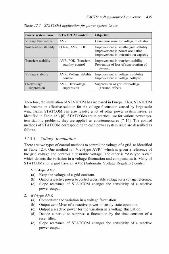
Therefore, the installation of STATCOM has increased in Europe. Thus, STATCOMhas become an effective solution for the voltage fluctuation caused by large-scalewind farms. STATCOM can also resolve a lot of other power system issues, asidentified in Table 12.3 [6]. STATCOMs are in practical use for various power sys-tem stability problems; they are applied as countermeasures [7–16]. The controlmethods of STATCOM corresponding to each power system issue are described asfollows.

12.3.1 Voltage fluctuationThere are two types of control methods to control the voltage of a grid, as identifiedin Table 12.4. One method is ‘‘Vref-type AVR’’ which is given a reference ofthe grid voltage and controls a desirable voltage. The other is ‘‘DV-type AVR’’which detects the variation in a voltage fluctuation and compensates it. Many ofSTATCOMs for a grid have an AVR (Automatic Voltage Regulator) control.

1. Vref-type AVR(a) Keep the voltage of a grid constant.(b) Output a reactive power to control a desirable voltage for a voltage reference.(c) Slope reactance of STATCOM changes the sensitivity of a reactive

power output.

2. DV-type AVR(a) Compensate the variation in a voltage fluctuation.(b) Output zero Mvar of a reactive power in steady-state operation.(c) Output a reactive power for the variation in a voltage fluctuation.(d) Decide a period to suppress a fluctuation by the time constant of a

reset filter.(e) Slope reactance of STATCOM changes the sensitivity of a reactive

power output.

Table 12.3 STATCOM application for power system issues

Power system issue STATCOM control Objective

Voltage fluctuation AVR Countermeasure for voltage fluctuation

Small-signal stability Q bias, AVR, POD Improvement in small-signal stabilityImprovement in power oscillationImprovement in transmission capacity

Transient stability AVR, POD, Transientstability control

Improvement in transient stabilityPrevention of loss of synchronism of

generator

Voltage stability AVR, Voltage stabilitycontrol

Improvement in voltage instabilityImprovement in voltage collapse

Overvoltagesuppression

AVR, Overvoltagesuppression

Suppression of grid overvoltage(Ferranti effect)


12.3.2 Small-signal stabilityThere is a small-signal stability constraint under heavy power flow on a long-distancetransmission line, and the desirable power cannot be transmitted [7–9]. STATCOMcan improve small-signal stability in this condition. Controls of AVR, POD (poweroscillation damping), and Q bias, as shown in Table 12.5, are applied to the controlsystem of STATCOM in order to improve the small-signal stability. The combinationof AVR, POD, and Q bias can enhance the effect on the small-signal stability.

1. Q bias control(a) Output a reactive power according to a reference of a reactive power or

current.(b) Improve small-signal stability and transmission capacity by providing a

reactive power constantly under heavy power flow.

2. AVR(a) Maintain synchronism of a grid with a reactive power output.(b) Detect a voltage drop with heavy load and compensate a voltage deviation.(c) Vref-type AVR and DV-type AVR can be applicable.

3. POD(a) Detect a power system oscillation inherent in a characteristic of a grid.(b) Improve damping power of a grid with a reactive power.

4. Application to small-signal stability

An example of STATCOM application to improve small-signal stability is450 MVA STATCOM installed at Toshin substation of Chubu Electric in Japan. Herea newly installed, large-capacity thermal power plant is connected to the main powergrid through 500 and 275 kV transmission lines. When one circuit of the transmissionlines that consists of long-distance double circuits is opened, small-signal stability

Table 12.4 Voltage control method

Control block diagram Voltage-reactive power characteristic

Vref-typeAVR

ΔV-typeAVR

∆V

TS1+TS

K1+T1S

K1+T1S

Reactivecurrent output

Reactivecurrent output

Q

Operating pointGrid characteristic

Q

VSlope

reactance

Grid characteristic

V

Operation areafor steady-state

Operation areafor transient

Operating point

V detection

V detection

V reference

+−


problems may occur because of loss of synchronism. The 450 MVA STATCOMimproves small-signal stability of this grid. Figure 12.3(a) shows the characteristicof voltage-reactive power of the STATCOM. As one circuit of a transmission lineis opened, small-signal instability occurs without STATCOM but STATCOM canimprove small-signal stability, as identified in Figure 12.3(b).

(a) Voltage-reactive power of characteristics of STATCOM.(b) Small-signal stability improvement in opening one circuit of transmission line.

12.3.3 Voltage stabilityA heavy load on transmission lines may cause voltage instability and voltage col-lapse [10–12]. A long-term planning stop or a retirement of generators willdecrease an upthrust of power flow from a load side and become a heavy load, andvoltage stability problems may occur. A P–V curve is used as an index of voltagestability. STATCOM can enhance the P–V curve in P-axis direction as identified inFigure 12.4. When one circuit is opened in double circuits of a transmission line,the P–V curve will change rapidly and voltage instability will occur. In such a case,an effect to avoid the voltage instability or voltage collapse can be expected by fastresponse of STATCOM. When STATCOM has a coordination control with a loadtap changer or shunt devices (shunt reactors and shunt capacitors), STATCOM canbe more effective for voltage stability.

Table 12.5 Control of small-signal stability improvement

Control block diagram Controlled object [17]

• increase in rotor angle through a nonoscillatory mode due to lack of synchronizing torque

• increase in rotor angle through a nonoscillatory mode due to lack of synchronizing torque

• rotor oscillations of increasing amplitude due to lack of sufficient damping torque

• rotor oscillations of increasing amplitude due to lack of sufficient damping torque

Q bias

AVR

POD

Q reference

V reference

Power flow

V detection

AVR

POD

Q biascontrol

Reactive currentreference ofSTATCOM



+−


1. AVR(a) Compensate voltage drop.(b) Keep a grid voltage constant, and enhance P–V curve and improve vol-

tage stability.(c) Compensate voltage drop rapidly by one circuit outage on a heavy load

and improve voltage stability.

2. Coordination control with load tap changer of transformer(a) Need to allow a leading reactive power output margin for prevention of

voltage collapse by one circuit outage on heavy load.(b) When AVR keeps a grid voltage constant, STATCOM outputs the reac-

tive power and it may not be the enough margin of the reactive power to

Capacitive

0(a)

–0.2000 2 4 6 8 10

(b)

T(s)

T(s)

10

20

30

40

Phase angle of Joestu generator Reactive power of each STATCOM50

Δq(deg)

–0.15–0.10–0.05

00.050.100.150.20Q(pu)

Reactive

VL

Dead band

AVR slopeVoltage

VU

STATCOM-1STATCOM-2

Var of each STATCOM

1pu = 1,000 MVA

without STATCOM

Q: Var of STATCOMs

with STATCOMs

2 4 6 82 4 6 8 1010100

Figure 12.3 450 MVA STATCOM – Effect on small-signal stability and overvoltage:(a) Voltage-reactive power of characteristics of STATCOM;(b) Small-signal stability improvement in opening one circuit oftransmission line� IEEE 2010. Reprinted with permission from Fujii, T., Temma, K., Morishima, N.,Akedani, T., Shimonosono, T., Harada, H., ‘450MVA GCT-STATCOM for stabilityimprovement and over-voltage suppression’, IEEE Proceedings, June 2010


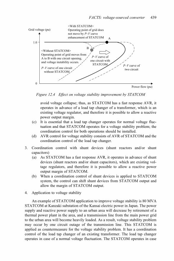
avoid voltage collapse; thus, as STATCOM has a fast response AVR, itoperates in advance of a load tap changer of a transformer, which is anexisting voltage regulator, and therefore it is possible to allow a reactivepower output margin.

(c) It is essential that a load tap changer operates for normal voltage fluc-tuation and that STATCOM operates for a voltage stability problem; thecoordination control for both operations should be installed.

(d) AVR control for voltage stability consists of AVR of STATCOM and thecoordination control of the load tap changer.

3. Coordination control with shunt devices (shunt reactors and/or shuntcapacitors)(a) As STATCOM has a fast response AVR, it operates in advance of shunt

devices (shunt reactors and/or shunt capacitors), which are existing vol-tage regulators, and therefore it is possible to allow a reactive poweroutput margin of STATCOM.

(b) When a coordination control of shunt devices is applied to STATCOMsystem, the control can shift shunt devices from STATCOM output andallow the margin of STATCOM output.

4. Application to voltage stability

An example of STATCOM application to improve voltage stability is 80 MVASTATCOM at Kanzaki substation of the Kansai electric power in Japan. The powersupply and reactive power supply to an urban area will decrease by retirement of athermal power plant in the area, and a transmission line from the main power gridto the urban area will become heavily loaded. As a result, voltage stability problemmay occur by one circuit outage of the transmission line. This STATCOM isapplied as countermeasure for the voltage stability problem. It has a coordinationcontrol of the load tap changer of an existing transformer. The load tap changeroperates in case of a normal voltage fluctuation. The STATCOM operates in case

0

1.0

Grid voltage (pu)<With STATCOM>Operating point of grid doesnot move by P–V curveenhancement of STATCOM

<Without STATCOM>Operating point of grid moves fromA to B with one circuit opening,and voltage instability occurs.

P–V curve of one circuitwithout STATCOM

P–V curve ofone circuit with

STATCOM

A

B

P–V curve oftwo circuit

Power flow (pu)

Figure 12.4 Effect on voltage stability improvement by STATCOM


of one circuit outage and it supplies reactive power in order to avoid voltageinstability and voltage collapse. Figure 12.5 shows voltage-reactive power (V–Q)characteristic of the STATCOM and the effect on power grid by STATCOMinstallation. STATCOM enhances the P–V curve in P-axis direction.

(a) V–Q (voltage-reactive power) characteristic of STATCOM.(b) Effect on P–V curve by STATCOM.

(a)

(b)

Q(pu)

Heavy slope

∆V(pu)Low slope 0.01

0.10

V(pu) P–V curve at A S/S 77 kV bus

0.0

0.2

0.4

0.6

0.8

1.0

1.2

0.15 0.20 0.25 0.30 0.35P(pu)

1.0

Figure 12.5 STATCOM for voltage stability: (a) V–Q (voltage-reactive power)characteristic of STATCOM; (b) Effect on P–V curve by STATCOM� IEEJ 2004. Reprinted with permission from ‘Improvement of voltage stabilitywith STATCOM’, Proceedings of Technical Meeting on Power Engineering ofIEEJ, PE-04-1, pp. 1–6, 2004


12.3.4 Transient stabilitySTATCOM is a new countermeasure for transient stability problem [13, 14]. Thefast response of STATCOM can avoid first swing instability or nth swing instabilityof generators. A control of transient stability improvement of STATCOM is calledpower system stabilizer (PSS) or power oscillation damping (POD). The controlperceives the state of power oscillation of the grid by detecting power flow oftransmission lines. STATCOM supplies the reactive power to the grid to control theacceleration and the deceleration of generators according to the control, and canimprove transient stability.

1. AVR(a) Compensate voltage drop due to large disturbance and maintain

synchronism.(b) Avoid first swing instability of generators.(c) Compensate voltage fluctuation of power oscillation after large disturbance.

2. PSS/POD(a) Detect power flow fluctuation.(b) Control damping corresponding to power oscillation.(c) Improve damping power of generators and avoid loss of synchronism.(d) AVR output and PSS/POD output are references of reactive current of

STATCOM.

3. Coordination control(a) Coordinate within two controls, AVR and PSS/POD, as identified in

Figure 12.6.(b) Actualize optimal transient stability improvement.(c) Depend on power system configuration and state.(d) Need to be customized according to power system characteristic.

4. Application to transient stability

Bus voltage AVR

PSS STATCOM output

Coordination controlfor transient stability

Power flow

Figure 12.6 Example of control of transient stability improvement


An example of STATCOM application to improve transient stability is130-MVA STATCOM installed at Inuyama substation of the Kansai electric powerin Japan. The objectives of the STATCOM are prevention of first swing instabilityand loss of synchronism. When AVR, PSS, and coordination control are applied tothe STATCOM, it can improve transient stability. The capacity for transient sta-bility is 130 MVA. As identified in Figure 12.7, first swing instability occurs by alarge disturbance without STATCOM. However, first swing instability can beavoided and transient stability improved with STATCOM.

12.3.5 Overvoltage suppressionCountermeasure for overvoltage suppression is basically a method similar to coun-termeasure for voltage fluctuation, and STATCOM absorbs reactive power rapidlyby AVR and suppresses overvoltage [7–9]. Either Vref-type AVR or DV-type AVRcan be applied to STATCOM for overvoltage suppression. Furthermore, currentforcing control can be applied to very fast overvoltage suppression. Figure 12.8 is anexample of AVR in combination with current forcing control.

0 2 4 6 8 1010

0 2 4 6 8 10(s)0.4

0.60.81.01.21.4V (pu) Bus voltage connecting to STATCOM

With STATCOM

With STATCOM

Without STATCOM

Without STATCOM

Without STATCOM

With STATCOM

0 2 4 6 8 10(s)

(s)

0306090

120150180

Angle (degree) Phase angle of generator

0 2 4 6 8 10

–0.4

–0.2

0.0

0.2

0.4Q (pu) Reactive power output of STATCOM

Figure 12.7 Effect on transient stability improvement by STATCOM� IEEJ 2011. Reprinted with permission from ‘Development of STATCOMfor transient stability improvement’, Proceedings of Technical Meeting on PowerEngineering of IEEJ, PE-11-187, pp. 27–30, 2011


1. AVR(a) Detect overvoltage and suppress overvoltage.(b) Decide the output corresponding to the volume of voltage drop or voltage

fluctuation.

2. Current forcing control(a) Fast response and fast overvoltage suppression compared to AVR.(b) Detect overvoltage and output required reactive current.

3. Application to overvoltage suppression

An example of STATCOM application to suppress overvoltage is 450 MVASTATCOM at Toshin substation as previously mentioned. One of the objectives ofthe STATCOM is overvoltage suppression. Many shunt capacitors are installed inthe grid where STATCOM is installed in order to compensate the reactive powerlosses of long-distance transmission lines on heavy load. It is possible that Ferrantiphenomenon occurs by large disturbance because of isolated power grid that con-sists of generators, long-distance transmission lines, and many shunt capacitors.The overvoltage suppression control is applied to the STATCOM and can suppressovervoltage, as identified in Figure 12.9.

High-speedvoltage

detection

Voltagedetection

Forcing currentreference

Selector Currentcontrol PWM

AVRBus voltage

Figure 12.8 Control block diagram of overvoltage suppression

0.00.50

0.75

1.00

1.25

1.50

1.75

2.00Voltage (pu) Maximum overvoltage in power grid Q(pu) Total reactive power output of STATCOMs

–0.6

–0.4

–0.2

0.0

0.2

0.4

0.6

0.2 0.4 0.6 0.8 1.0T(s)

T(s)0.00.0 0.20.2 0.40.4 0.60.6 0.80.8 1.01.00.0 0.2 0.4 0.6 0.8 1.0

Overvoltage by Ferranti effect

Overvoltage suppression

Fast Q output

Figure 12.9 Effect on overvoltage suppression by 450 MVA STATCOM� IEEE 2010. Reprinted with permission from Fujii, T., Temma, K., Morishima, N.,Akedani, T., Shimonosono, T., Harada, H., ‘450MVA GCT-STATCOM for stabilityimprovement and over-voltage suppression’, IEEE Proceedings, June 2010


12.4 High-order harmonic resonance phenomena

FACTS, which uses a VSC such as STATCOM, generates theoretical harmonics byswitching of pulse width modulation (PWM) control. The harmonics are wellknown. Since the calculation procedures and the review methods are established,the harmonics generated at a grid connection point of STATCOM can be theore-tically predicted in advance. However, as STATCOM is applied to a power grid, anunknown harmonic resonance phenomenon may occur. A high-order harmonicresonance phenomenon [18] is introduced in this section.

This high-order harmonic resonance phenomenon is identified by studyingSTATCOM installation. Furthermore, the mechanism of the harmonic resonancephenomenon is clarified. It has been generally estimated that this high-order har-monics would be damped immediately and would not cause any harmonic pro-blems. However, it has been verified by field tests on an actual STATCOMinstallation that the resonance phenomenon occurs and is a practical matter to bedealt with. The resonance phenomenon can be estimated by EMTP analysis.Countermeasures for the resonance phenomenon are also identified.

12.4.1 Overview of high-order harmonic resonance phenomenonSTATCOM produces a voltage of substantially sinusoidal waveform by switching DCvoltage with gate turn off (GTO) thyristor, gate commutated turn-off (GCT) thyristor,or insulated gate bipolar transistor (IGBT) devices. The voltage waveform which issubstantially sinusoidal waveform without lower harmonics can be generated bywaveform synthesis with a PWM control, either with or without a multiple convertertransformer. However, the higher frequency harmonics are still generated in both cases.

12.4.1.1 Harmonics of a voltage-sourced converterHarmonics of three-phase VSCs using PWM control are given by (12.1) and (12.2).

Vf 0 ¼ffiffiffi3

p

2aEd

Vfh ¼ffiffiffi3

p

24Ed

npJk

anp2

� � ð12:1Þ

where:

Vf 0: amplitude of the fundamental-frequency w0 componentVfh: amplitude of the fundamental-frequency nws � kw0 component:

k ¼ 3ð2m � 1Þ � 1; m ¼ 1; 2; � � � ðn ¼ 1; 3; 5; � � �Þ

k ¼ 6m þ 1;

6m � 1;

(m ¼ 0; 1; � � �m ¼ 1; 2; � � � ðn ¼ 2; 4; 6; � � �Þ ð12:2Þ

Jk: k-th order Bessel functiona: amplitude modulation ratio of VSC

Ed: DC voltage of VSCw0: angular frequency of control signalws: angular frequency of carrier signal


Various harmonic orders are included in the total harmonic voltage of STATCOM.A constant dead time ‘‘Td’’ between an on-pulse and an off-pulse has an influenceon the various harmonic orders, but Td is necessary to prevent failure of switchingdevices. Therefore, a VSC will generate a lot of small harmonics in the range of alower to higher order.

When the VSC is connected to a grid that has resonant and anti-resonantcharacteristics, the harmonics from the VSC may be magnified and have a negativeimpact on the grid.

Figure 12.10 illustrates a sample circuit for high-order harmonic resonancephenomenon. A VSC system such as STATCOM that consists of a VSC and thegrid connection point of the VSC system is the tertiary side of an existing powertransformer of grid through a cable. The length of the cable is about 500 m.Table 12.6 lists the parameters of the sample circuit. Harmonic voltages of the VSCsystem are reduced by shifting each phase of the switching pulses of each four-stage converter through the multiple converter transformer.

12.4.1.2 EMTP analysis of high-order harmonic resonanceElectromagnetic transient program (EMTP) analysis is performed. The VSC isconnected to the grid as illustrated in Figure 12.10 in the analysis. Here, the laggingreactive power output of the VSC is set to 37.5 Mvar. Very high order harmonicsare included in the voltage (Vh) on the primary side of the multiple convertertransformer, as identified by the EMTP results shown in Figure 12.11. A fastFourier transform (FFT) of EMTP is performed in order to analyze the voltage Vh

in detail with the high-order harmonics on the primary side of the convertertransformer. The FFT results of high-order harmonics are listed in Table 12.7. Theharmonics around the 130th order is the most significant one.

When the VSC system is disconnected from the existing transformer ofFigure 12.10 and the VSC, only the converter transformer and the cable remain;

Existingtransformer

Cable

Multipletransformer VSC

VSC system

Figure 12.10 Voltage-sourced converter system and power transformer of grid� IEEE 2005. Reprinted with permission from Temma, K., Ishiguro, F.,Toki, N., Iyoda, I., Paserba, J.J., ‘Clarification and measurements of high frequencyharmonic resonance by a voltage sourced converter’, IEEE Transactions on PowerDelivery, vol. 20, no. 1, January 2005


harmonic voltages generated from the VSC on the primary side of the convertertransformer are analyzed (Vho). Table 12.8 lists the result of the FFT analysis.

As listed in Table 12.7, the ratios Vh/V0 of each harmonic voltage Vh on theprimary side of the multiple converter transformer range from 0.34% to 4.16% offundamental voltage with the connection to the grid. As listed in Table 12.8, theratios Vho/V0 of each harmonic voltage Vho on the primary side of the multipleconverter transformer range from 0.2% to 3.74% of fundamental voltage withoutconnection to the grid. The results indicate that the ratios of both sets of results areapproximately the same. However, when the magnified ratios of the two conditions(column labeled Vh/Vho in Table 12.8) are examined, it is verified that the harmonicvoltages of the 131st to 139th order are magnified with the connection of the VSCto the grid. The magnified ratio Vh/Vho of 135th harmonic voltage is the largestfound here and is nearly 24 times.

12.4.1.3 Frequency–impedance ( f–Z ) characteristics of gridBased on the observations of FFT results as described previously, it is assumed thata series and a parallel resonant circuit exist in this grid since the amplitude of theharmonic voltages near the 130th order is magnified in the EMTP simulationresults. Furthermore, frequency-domain analysis is performed in order to investigatethis phenomenon. This is accomplished in two stages. The VSC is replaced with acurrent source at the first stage. Then frequency versus impedance ( f–Z ) character-istics of the grid can be calculated as viewed from the secondary side of the convertertransformer by varying the frequency of injected current over a range of interests. Atthe second stage, the VSC and the converter transformer are replaced by a currentsource. The f–Z characteristics as viewed from the primary side of the convertertransformer can be calculated in the same way. Figure 12.12 illustrates the concept.

Table 12.6 Parameters of sample circuit

Cable type CVT 3 � 500

Cable length 500 m

VSC capacity 53 MVA

PWM control for VSC Nine-pulse PWM

Main circuit configuration of VSC Three-phase converter

Number of multiple stage of converter transformer Four stage

Voltage ratio of converter transformer 66 kV/4.6 kV

Connection of converter transformer Y-D

%L – Inductance of converter transformer 20%

� IEEE 2005. Reprinted with permission from Temma, K., Ishiguro, F., Toki, N.,Iyoda, I., Paserba, J.J., ‘Clarification and measurements of high frequency harmonicresonance by a voltage sourced converter’, IEEE Transactions on Power Delivery,vol. 20, no. 1, January 2005


Figure 12.13 shows the results of f–Z viewed from the primary side andFigure 12.14 shows the results of f–Z viewed from the secondary side. From thesefigures we can make the following observations:

1. f–Z characteristics from the primary side: A parallel resonant exists in thiscircuit and the parallel resonance point is 130.1th. The resonance impedance is267.3 kW.

2. f–Z characteristics from the secondary side: A series resonant exists in this circuitand the series resonance point is 135.8th. The resonance impedance is 23.8 W.

It is verified that a series resonant circuit and a parallel resonant circuit existwithin a very narrow frequency band near the 130th harmonic in this frequencydomain analysis.

–60–40–20

204060Voltage (kV) The phase voltage at the primary side of Tr of VSC

0 Time (ms)

PhaseAPhaseAPhaseBPhaseBPhaseCPhaseC

–120–80–40

4080

120Voltage (kV) The phase-phase voltage at the primary side of Tr of VSC

0 Time (ms)400400 405405 410410 415415 420420400 405 410 415 420

–0.6–0.4–0.2

0.20.40.6Current (kA) The current at the primary side of Tr of VSC

0.0 Time (ms)

400400 405405 410410 415415 420420400 405 410 415 420

Phase-APhase-BPhase-C





400400 405405 410410 415415 420420400 405 410 415 420

Figure 12.11 EMTP result of voltage and current on primary side of convertertransformer� IEEE 2005. Reprinted with permission from Temma, K., Ishiguro, F., Toki, N.,Iyoda, I., Paserba, J.J., ‘Clarification and measurements of high frequency harmonicresonance by a voltage sourced converter’, IEEE Transactions on Power Delivery,vol. 20, no. 1, January 2005


Table 12.8 Result of FFT of EMTP simulations ofvoltage ( Vh ) and current ( Ih ) on primaryside of converter transformer withoutconnection to grid

Harmonic order Primary voltage of transformer Vh

VhoVho [%] Vho /V0 [%]a

119th 1,653.0 3.74 0.35

121st 502.7 1.14 0.35

131st 1,651.0 3.73 1.32

133rd 867.4 1.96 2.46

135th 87.6 0.20 23.58

137th 136.9 0.31 4.71

139th 1,083.0 2.45 1.40

143rd 1,133.0 2.56 0.73

145th 1,243.0 2.81 0.52

aV0, fundamental wave of voltage.� IEEE 2005. Reprinted with permission from Temma, K., Ishiguro, F.,Toki, N., Iyoda, I., Paserba, J.J., ‘Clarification and measurements of highfrequency harmonic resonance by a voltage sourced converter’, IEEETransactions on Power Delivery, vol. 20, no. 1, January 2005

Table 12.7 Result of FFT of EMTP simulations of voltage ( Vh ) and current ( Ih )on primary side of converter transformer with connection to grid

Harmonicorder

Primary voltage of transformer Primary current of transformer

Vh [V] Vh/V0 [%]a Ih [A] Ih / I0 [%]a

119th 574.3 1.10 0.55 0.11

121st 176.0 0.34 0.16 0.03

131st 2,179.8 4.16 0.25 0.05

133rd 2,134.1 4.08 0.58 0.11

135th 2,065.2 3.95 0.89 0.18

137th 644.7 1.23 0.34 0.07

139th 1,519.7 2.91 1.13 0.23

143rd 829.7 1.59 0.83 0.17

145th 642.4 1.23 0.79 0.16

aV0, I0: fundamental wave of voltage and current.� IEEE 2005. Reprinted with permission from Temma, K., Ishiguro, F., Toki, N., Iyoda, I., Paserba, J.J.,‘Clarification and measurements of high frequency harmonic resonance by a voltage sourced converter’,IEEE Transactions on Power Delivery, vol. 20, no. 1, January 2005


Existingtransformer

f–Z characteristicsfrom primary side

f–Z characteristicsfrom secondary side

Multipletransformer

VSC

Figure 12.12 Frequency–impedance characteristics for power system� IEEE 2005. Reprinted with permission from Temma, K., Ishiguro, F., Toki, N.,Iyoda, I., Paserba, J.J., ‘Clarification and measurements of high frequency harmonicresonance by a voltage sourced converter’, IEEE Transactions on Power Delivery,vol. 20, no. 1, January 2005

5,5000

10

20

30

40

50Impedance (kΩ) Frequency–impedance ( f–Z ) characteristics

6,000 6,500 7,000 7,500 8,000Frequency (Hz)

1240123456

Impedance (kΩ) Close-up near 6,500 Hz

126 128 130 132 134 136 138 140Frequency (order)

133rd: 4,434 Ω

133rd: 2,617 Ω

Parallel resonance: 130.1th

Figure 12.13 Frequency-impedance ( f–Z) characteristics as viewed from theprimary side of the converter transformer by EMTP results� IEEE 2005. Reprinted with permission from Temma, K., Ishiguro, F., Toki, N.,Iyoda, I., Paserba, J.J., ‘Clarification and measurements of high frequency harmonicresonance by a voltage sourced converter’, IEEE Transactions on Power Delivery,vol. 20, no. 1, January 2005


12.4.1.4 Correlation between impedance and harmonic voltageThe values Zh of Nth-order impedance as viewed from the primary side of theconverter transformer are calculated by the frequency-domain simulation (i.e., f–Zcharacteristics as shown in Figure 12.13); the values are listed in Table 12.9.The results of Nth-order harmonic voltage Vh and harmonic current Ih calculated bythe time-domain analysis of Figure 12.11 are also listed in Table 12.9. Each productof Zh (from the frequency-domain analysis) times Ih (from the time-domain ana-lysis) is approximately equal to Vh (from the time domain analysis), which is listedin the last column of Table 12.9. Therefore, harmonic impedance Zh, harmoniccurrent Ih, and harmonic voltage Vh from the two different domain analyses have acorrelation with each other and it is verified that both time-domain and frequency-domain simulation results are appropriate.

12.4.2 Principle of high-order harmonic resonance phenomenonIt is presumed that the circuit in the vicinity of the VSC causes the high-orderharmonic resonance voltage as shown in Figure 12.10. A basic equivalent circuitthat consists of the VSC system, cables, and tertiary winding of the existingtransformer in the grid is applied to the analysis presented here.

The basic equivalent circuit that defines the phenomenon consists of theleakage inductance L1 of the converter transformer, the capacitance C of the cable,

5,500 6,000 6,500 7,000 7,500 8,0000

10

20

30

40

50Impedance (kΩ) Frequency–impedance ( f–Z ) characteristics

Frequency (Hz)

1240123456

Impedance (kΩ) Close-up near 6,500 Hz

126 128 130 132 134 136 138 140Frequency (order)

Series resonance: 135.8th

Figure 12.14 Frequency-impedance ( f–Z) characteristics as viewed from thesecondary side of the converter transformer by EMTP results� IEEE 2005. Reprinted with permission from Temma, K., Ishiguro, F., Toki, N.,Iyoda, I., Paserba, J.J., ‘Clarification and measurements of high frequency harmonicresonance by a voltage sourced converter’, IEEE Transactions on Power Delivery,vol. 20, no. 1, January 2005


the leakage inductance L2 of the tertiary winding of the existing transformer, andthe VSC as illustrated in Figure 12.15.

The basic equivalent circuit close to the VSC system has a series resonant circuitand a parallel circuit. The equivalent impedance Zeq of the circuit is given by (12.3).

Zeq ¼ jXeq ¼ jwL2 þ wL1 1 � w2L2Cð Þ

1 � w2L2C

� �ð12:3Þ

The condition of series resonance is that the equivalent reactance Xeq of the circuitis zero.

wL2 ¼ wL1 1 � w2L2C� � ¼ 0 ð12:4Þ

Table 12.9 Correlation between Nth order harmonic voltage and Nthorder impedance

Harmonicorder

Vh [V]Time-domain

Ih [A]Time-domain

Zh [W]Frequency-domain

Zh�Ih [V]

119th 574.3 0.55 1,067 585.9

121st 176.0 0.16 1,319 211.0

131st 2,179.8 0.25 15,008 3,752.0

133rd 2,134.1 0.58 4,434 2,571.7

135th 2,065.2 0.89 2,617 2,329.1

137th 644.7 0.34 1,863 633.4

139th 1,519.7 1.13 1,450 1,638.5

143rd 829.7 0.83 1,009 837.5

145th 642.4 0.79 877 692.8

� IEEE 2005. Reprinted with permission from Temma, K., Ishiguro, F., Toki, N., Iyoda, I., Paserba, J.J.,‘Clarification and measurements of high frequency harmonic resonance by a voltage sourced converter’,IEEE Transactions on Power Delivery, vol. 20, no. 1, January 2005

Tertiary leakageinductance of existing

transformer

Capacitanceof cable

Leakage inductanceof multiple transformer

VSC

L1L2

C

Figure 12.15 Basic equivalent circuit close to voltage-sourced converter system� IEEE 2005. Reprinted with permission from Temma, K., Ishiguro, F., Toki, N.,Iyoda, I., Paserba, J.J., ‘Clarification and measurements of high frequency harmonicresonance by a voltage sourced converter’, IEEE Transactions on Power Delivery,vol. 20, no. 1, January 2005


The series resonance frequency fser is as follows:

fser ¼ 1

2pffiffiffiffiffiffiffiffiffiffiffiffiffiffiffiL1L2C

L1 þ L2

r ¼ 6;962 Hz ¼ 139:3th ð12:5Þ

Furthermore, the condition of parallel resonance is that the equivalent reac-tance Xeq of the circuit is infinite.

1 � w2L2C ¼ 0 ð12:6ÞThe parallel resonance frequency fpar is as follows:

fpar ¼ 1

2pffiffiffiffiffiffiffiffiL2C

p ¼ 6;681 Hz ¼ 133:6th ð12:7Þ

where the leakage impedance of the tertiary winding of the existing transformer is%Zt ¼ 32.8% on a 1,000 MVA base.

When the sample circuit of Figure 12.10 is modeled in detail and performed byEMTP, the series resonance frequency fser is 135.8th and the parallel resonancefrequency fpar is 130.1th. Each result of the EMTP analysis corresponds to eachanalytical result of (12.5) and (12.7) approximately. Therefore, it is verified that thefundamental principle of the series resonance and the parallel resonance occurs bymeans of the circuit elements of the basic equivalent circuit of Figure 12.15,namely the leakage inductance L1 of the converter transformer, the capacitance Cof the cable, and the leakage inductance L2 of the tertiary winding of the existingtransformer.

The series resonance frequency fser calculated by the detailed circuit(Figure 12.10) is 135.8th. At first, a series resonance occurs when the voltagegenerated from the VSC includes around 135th order harmonic voltage. The seriesresonance magnifies a harmonic current Iln generated from the VSC on the sec-ondary side of the converter transformer. The harmonic current Iln on the secondaryside of the converter transformer (L1) is equal to a harmonic current Ihn on theprimary side of the converter transformer (L1) as illustrated in Figure 12.16. Then,the 131st order parallel resonance exists in the f–Z characteristic viewed from theprimary side of the converter transformer. An impedance Zhn around the 135th isclose to the 131st. Since the voltage on the primary side of the converter trans-former is determined by Zhn � Ihn and with both Zhn and Ihn around the 135thharmonic magnified, then the 135th order harmonic voltage is magnified.

Therefore, it is clarified that the principle of the high-order harmonic reso-nance phenomenon is as follows:

1. When a very small harmonic voltage is generated from a VSC on the secondaryside of the multiple converter transformer, a series resonance that exists in thefrequency close to the small harmonic voltage magnifies a harmonic current.

2. The magnified current on secondary side of the converter transformer flows tothe primary side through its leakage reactance.


3. When a parallel resonance frequency is close to the series resonance frequency,a large harmonic voltage could occur by the magnified current and the reso-nance impedance of these resonant circuits.

12.4.3 Field test12.4.3.1 Field test conditionIn order to verify the high-order harmonic resonance phenomenon, a field test forthe phenomenon is performed. A 53 MVA VSC system with a 4-stage-multipleconverter transformer is connected to a tertiary side of an existing transformerthrough a cable 500 meters long, in common with the sample circuit of Figure 12.10.

12.4.3.2 Field test resultsThe phase voltage Vm1 and current Im1 are measured on the primary side of themultiple converter transformer when the reactive power outputs are þ37.5 Mvarand 0 Mvar respectively in a STATCOM operation mode for the condition. Themeasurements of the field test are shown in Figure 12.17. High frequency voltagesaround 130th are found on the primary side of the converter transformer as shownin the field test results of Figure 12.17.

These field test results show that a very small harmonic voltage is magnifiedby a series and parallel resonant circuits as clarified in the simulation and analyticalresults when a grid has the series and parallel resonant circuits and both resonantcircuits are close in frequency. Thus it is confirmed by analysis, simulation, andmeasurements that a high-order harmonic resonance phenomenon can occur and isa practical matter to be dealt with.

1. Voltage and current at VSC output Q ¼þ37.5 Mvar2. Voltage and current at VSC output Q ¼ 0 Mvar3. Enlarged view of voltage and current at VSC output Q ¼ 0 Mvar

axis: V¼ 20 kV/div, I¼ 300 A/div; horizontal axis: Time ¼ 5 ms/div (Figure 12.17(a)and (b)), Time ¼ 1 ms/div (Figure 12.17(c)).

L2 L1 Vln

VSC

Iln

Zhn

Vhn

Ihn

C

Figure 12.16 Series resonance and parallel resonance of high-order harmonicresonance� IEEE 2005. Reprinted with permission from Temma, K., Ishiguro, F., Toki, N.,Iyoda, I., Paserba, J.J., ‘Clarification and measurements of high frequency harmonicresonance by a voltage sourced converter’, IEEE Transactions on Power Delivery,vol. 20, no. 1, January 2005


V, Ib

Vertical axis: V = 20 kV/div, I = 300 A/div Horizontal axis: Time = 5 ms/div(a)

(b)

Ib

Ia

Ib

IcIc

V, Ib

Ia

Ic

V, Ib

Ia

Ib

V

Ic

Ia

V

Vertical axis: V = 20 kV/div, I = 300 A/div Horizontal axis: Time = 5 ms/div

(c)Vertical axis: V = 20 kV/div, I = 300 A/div Horizontal axis: Time = 1 ms/div

V

Figure 12.17 Measurement results of field test of 53 MVA voltage-sourcedconverter� IEEE 2005. Reprinted with permission from Temma, K., Ishiguro, F., Toki, N.,Iyoda, I., Paserba, J.J., ‘Clarification and measurements of high frequency harmonicresonance by a voltage sourced converter’, IEEE Transactions on Power Delivery,vol. 20, no. 1, January 2005


12.4.4 Considerations and countermeasuresHigh-order harmonic resonance phenomenon depends on a local condition at the gridconnection point of the VSC system. The local condition is caused by the series andparallel resonant circuit of the reactance of converter transformer, the capacitancesof cables, and the reactance of existing transformer. It has been considered in thepast that high-order harmonics are reduced immediately and no critical problemwill be caused. However, the advancements of technology has decreased theimpacts of the factors that reduce harmonics, such as losses of a cable and atransformer, in this case with VSC and PWM, therefore the problems have begun toactualize. Such phenomenon has been reported by some VSC-based systemsrecently. The influence on high-order harmonic resonance by the cable and coun-termeasures for them is described in this section.

12.4.4.1 Influence on phenomenon by length of cableA capacitance of a cable becomes larger as the cable length is longer. As the capaci-tance is larger, the orders of series resonance and parallel resonance move lower. Ingeneral, amplitude of a harmonic voltage tends to increase when the harmonic orderbecomes low. Therefore, it is assumed that the harmonics increase as a resonance pointtransitions to a low frequency. Simulations of the total harmonic distortion (THD) areperformed to show the impact of cable length. The THDs are the phase voltages on theprimary side of the multiple converter transformer illustrated in Figure 12.10. Theparameter of these simulations is the length of the cable. The results of the simulationsin Table 12.10 indicate that the THD of the voltage increases with the larger capaci-tance of the longer cable. It is verified that the magnitude of the high-order harmonicresonance tends to increase as the length of the cable becomes longer. It should benoted that the same phenomenon would occur for anything else that increases thecapacitance between the power system and the VSC such as cables in parallel.

When there is no cable between the existing transformer and the convertertransformer, there is no significant capacitance. It is assumed that the high-orderharmonic resonance phenomenon will not occur because of the absence of theresonant circuit. Figure 12.18 shows the simulation result with no cable. It isclarified that a capacitance of a cable is one of the causes of high-order harmonicresonance as confirmed in Figure 12.18. Thus, the resonance can be prevented from

Table 12.10 Relation between cable length and THD ofoutput voltage of VSC

Length (m) 0 200 390 500 700 900

THDa (%) 1.54 1.84 5.19 8.50 11.60 20.16

aTHD of harmonic voltages while connecting to grid.� IEEE 2005. Reprinted with permission from Temma, K., Ishiguro, F.,Toki, N., Iyoda, I., Paserba, J.J., ‘Clarification and measurements of highfrequency harmonic resonance by a voltage sourced converter’, IEEE Trans-actions on Power Delivery, vol. 20, no. 1, January 2005


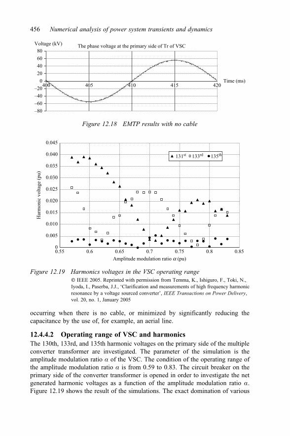
occurring when there is no cable, or minimized by significantly reducing thecapacitance by the use of, for example, an aerial line.

12.4.4.2 Operating range of VSC and harmonicsThe 130th, 133rd, and 135th harmonic voltages on the primary side of the multipleconverter transformer are investigated. The parameter of the simulation is theamplitude modulation ratio a of the VSC. The condition of the operating range ofthe amplitude modulation ratio a is from 0.59 to 0.83. The circuit breaker on theprimary side of the converter transformer is opened in order to investigate the netgenerated harmonic voltages as a function of the amplitude modulation ratio a.Figure 12.19 shows the result of the simulations. The exact domination of various

–80–60–40

406080

Voltage (kV) The phase voltage at the primary side of Tr of VSC

Time (ms)–20

200

420415410405400

Figure 12.18 EMTP results with no cable

131st 133rd 135th

0.550

0.005

0.010

0.015

0.020

0.025

0.030

0.035

0.040

0.045

0.6 0.65 0.7Amplitude modulation ratio a (pu)

Har

mon

ic v

olta

ge (p

u)

0.75 0.8 0.85

Figure 12.19 Harmonics voltages in the VSC operating range� IEEE 2005. Reprinted with permission from Temma, K., Ishiguro, F., Toki, N.,Iyoda, I., Paserba, J.J., ‘Clarification and measurements of high frequency harmonicresonance by a voltage sourced converter’, IEEE Transactions on Power Delivery,vol. 20, no. 1, January 2005


harmonic voltage orders is different through the examined range of a. However, thedominant harmonic voltages are all around the 130th order for the entire range of a.Therefore, this analysis shows that modifying the VSC control is not practical andeffective means to prevent this high-order harmonic resonance phenomenon.

12.4.4.3 Countermeasure for high-order harmonic resonanceIt is difficult to estimate the amount of high-order harmonics in the pre-manufacturing/design stages exactly. When small deviations of a leakage inductance of a transformeroccur or the exact length of cable may not be precisely defined in advance, the reso-nant and anti-resonant point may move and the amount of the high-order harmonicsmay change because of these reasons. Furthermore, it would be overly conservative toconsider the maximum conditions of the high-order harmonics and to design andmanufacture a multiple converter transformer, a cable, cable terminations, a powertransformer, protective relays, and the VSC to meet the potentially higher levels ofhigh-order harmonic and the respective impacts on insulation and control systems.

One of the countermeasures for the high-order harmonic resonance is to install aharmonic filter on the primary side of the converter transformer. The simulation ofthe THD of the harmonic voltages with the harmonic filter is performed. The impacton the constraint for high-order harmonic resonance phenomenon is verified and thecapacity of the harmonic filter can be estimated. The parameter of the simulation isthe capacity of the harmonic filter. The results for THD for the capacity of eachharmonic filter are shown in Table 12.11. The criterion of the THD of the harmonicvoltages is within 2%. A 1.5 to 2.0 MVA harmonic filter should be installedapproximately by simulation results.

Thus, it is evaluated that high-order harmonic resonance can be restricted by aharmonic filter with a relatively small capacity compared to the capacity of theVSC. The example filter size in this study is about 4% of the rating of the VSC.

The best method to avoid the resonance phenomenon in the field is to ade-quately perform a power system analysis in advance and to consider the accuracy ofpower system parameters used in the analysis.

References

[1] Hingorani N. G., ‘High power electronics and flexible AC transmissionsystem’, IEEE Power Engineering Review, vol. 8, no. 7. pp. 3–4, July 1988.

Table 12.11 Simulation results for harmonic voltage reductionby a high-pass filter

Capacity of high-pass Filter (MVA) 0 1.0 1.5 2.0

THD of harmonic voltage (%) 8.50 3.12 1.94 1.61

� IEEE 2005. Reprinted with permission from Temma, K., Ishiguro, F., Toki, N.,Iyoda, I., Paserba, J.J., ‘Clarification and measurements of high frequencyharmonic resonance by a voltage sourced converter’, IEEE Transactions onPower Delivery, vol. 20, no. 1, January 2005


[2] Mori S., ‘Initiatives perspectives by the power industry towards a low carbonemission society’, Keynote address of Paris Session CIGRE 2010.

[3] Yokoyama A., ‘Optimal control demonstration project for the next-generationtransmission and distribution system’, Electrical Review (Denki Hyoron),vol. 95, no. 10, pp. 26–29, 2010 (in Japanese).

[4] Dennis W., ‘Power electronics for wind energy applications’, presentation slideof IEEE northern Canada section, Edmonton, September 17, 2012.

[5] Hingorani N. G., Gyugyi L., Understanding FACTS: Concepts and Tech-nology of Flexible ac Transmission Systems, Wiley-IEEE Press, NJ, UnitedStates, 1999.

[6] Temma K., Kitayama M., ‘STATCOM technology for smart grid and thenext-generation transmission and distribution system’, Smart Grid (technicaljournal), April, pp. 8–12, 2012 (in Japanese).

[7] Akedani T., Hayashi J., Temma K., Morishima N., ‘450MVA STATCOMinstallation plan for stability improvement’, Proceeding of 2010 CIGRE,Paper B4-207, Paris Session 2010.

[8] Matsuda T., Shimonosono T., Harada H., Temma K., Morishima N.,Shimomura T., ‘Factory test and commissioning test of 450 MVA-STATCOMproject’, Proceeding of 2014 CIGRE, Paper B4-204, Paris Session 2014.

[9] Fujii T., Temma K., Morishima N., Akedani T., Shimonosono T., Harada H.,‘450MVA GCT-STATCOM for stability improvement and over-voltagesuppression’, International Power Electronics Conference, IEEJ, IPEC-Sapporo, Japan, pp. 1766–1772, 2010.

[10] Yagi M., Takano T., Sato T., Iyoda I., Temma K., ‘Role and new technol-ogies of STATCOM for flexible and low cost power system planning’,Proceedings of 2002 CIGRE, Paper SC14-107, Paris Session 2002.

[11] Yonezawa H., Imura H., Shinki Y., Temma K., Funahashi S., Teramoto H.,‘Improvement of voltage stability with STATCOM’, Proceedings of theTechnical Meeting on Power Engineering of IEEJ, PE-04-1, pp. 1–6, 2004(in Japanese).

[12] Sato T., Matsushita Y., Temma K., Morishima N., Iyoda I., ‘Prototype test ofSTATCOM and BTB based on voltage source converter using GCT thyr-istor’, Transmission and Distribution Conference and Exhibition 2002 AsiaPacific. IEEE/PES, pp. 2037–2042, 2002.

[13] Anjiki M., Nagatomo Y., Taketa K., Temma K., Masaki K., Fujii T.,Morishima N., ‘Development of STATCOM for transient stabilityimprovement’, Proceedings of the Technical Meeting on Power Engineeringof IEEJ, PE-11-187, pp. 27–30, 2011 (in Japanese).

[14] Imanishi T., Nagatomo Y., Iwasaki S., Masaki K., Fujii T., Ieda J., ‘130MVA-STATCOM for transient stability improvement’, International PowerElectronics Conference, IEEJ, IPEC-Hiroshima, Japan, pp. 2663–2667, 2014.

[15] Mori S., Matsuno K., Hasegawa T., Ohnishi S., Takeda M., Seto M.,Murakami S., Ishiguro F., ‘Development of a large static VAr generatorusing self-commutated inverters for improving power system stability’,IEEE Transactions on Power Systems, vol. 8, pp. 371–377, 1993.


[16] Reed G., Paserba J., Croasdaile T., Takeda M., Hamasaki Y., Aritsuka T.,Morishima N., . . . Haas D., ‘The VELCO STATCOM-based transmissionsystem project’, 2001 IEEE PES WM, vol. 3, pp. 1109–1114, 2001.

[17] Kundur P., Paserba J., Ajjarapu V., Andersson G., Bose A., Canizares C.,Hatziargyriou N. . . . Vittal V., ‘Definition and classification of power systemstability’, IEEE/CIGRE joint task force on stability terms and definitions.IEEE Transactions on Power Systems, vol. 19, no. 3, pp. 1387–1401, 2004.

[18] Temma K., Ishiguro F., Toki N., Iyoda I., Paserba J. J., ‘Clarification andmeasurements of high frequency harmonic resonance by a voltage sourcedconverter’, IEEE Transactions on Power Delivery, vol. 20, pp. 450–457,2005.


Chapter 13

Application of SVC to cable systems

Y. Tamura*

13.1 AC cable interconnection to an island

Interconnection to the island from the mainland has advantages as follows. Theelectric power on remote islands, in general, has been provided by power genera-tion on the islands, which requires maintenance and fuel transport for the gen-erators. If the mainland and the remote island are connected by submarine cablesand power is transmitted from the mainland, there are economic advantages sincethe costs of maintenance and fuel for generators on the island can be reduced.

However, in long-distance AC cable power transmission, voltage problemssuch as variations on the load side caused by the capacitance of the cable andharmonic resonance phenomena must be resolved [1–8]. Among these problems,voltage variation on the load side caused by switching on and off the long-distanceAC cable cannot be ignored.

The Kyushu Goto Island chain was connected to the mainland and operationstarted through 66 kV AC cables in 2005 as illustrated in Figure 13.1. The short-circuit capacitance of the Goto Island system is several hundred megavolt amperes,while the 66 kV AC cable linked to the mainland has a capacitance of approximately20 Mvar per one circuit. Therefore, voltage variations occur on the island as a resultof switching one circuit on or off. In particular, in case if fault occurs, the existingvoltage regulation equipment such as transformer taps or phase-modifying equipmentcontrol cannot suppress the voltage variation immediately because of slow response.Thus, an Static Var Compensator (SVC) was installed in the Okuura switching stationon Fukue Island in the Goto Islands as illustrated in Figure 13.1 [9, 10].

13.2 Typical example of voltage variations in an island

The causes of voltage variations include transmission line faults on an island, tapcontrol in a transformer linked to the mainland, and phase-modifying equipmentcontrol on an island. The greatest voltage variations occur when switching on or offone circuit of the AC cables linked to the mainland. Figure 13.2 shows an example of

*Senior Engineer, Toshiba Co., Japan

voltage variations on an island. This waveform is a calculated example for a voltage of66 kV at the Okuura switching station without the SVC, using an analysis model to bedescribed below. When a fault is detected in an overhead transmission line segmentamong two circuits of the 66 kV interconnection to the mainland, the circuit whichincludes faulty overhead transmission line is opened at both ends of the inter-connection line including the cable segment. Then the circuit is reconnected after 60seconds. In this example, the voltage after the cable is disconnected drops by 17.2%,

Naru SS

Fukue No2 PS

Wanigawa PS

Nihonkusu SS

Hisaka SS

Narao SS

Shin-Arikawa PS

Ojika SS

Uku PS

Matsushima PS

Kita-Nagasaki SS

Higashi-Sasebo SS

66 kV Matsushima-Naraoline (2cct) 54 kmOkuura SWS/SVC

Azetsu SS

Urakuwa SSGoto islands

Kyusyu main island

Matsushima-SS

Marusebana connection

Figure 13.1 Interconnection from the mainland to the island� 2013 Wiley Periodicals, Inc. Reprinted with permission from Yuji Tamura,Shinji Takasaki, Yasuyuki Miyazaki, Hideo Takeda, Shoichi Irokawa, Kikuo Takagi,Naoto Nagaoka, ‘Voltage control of static var compensator for a remote systeminterconnected by long-distance AC cables’, Electrical Engineering in Japan,pp. 19–30, November 2013

0 100 200 300 400 500 6000.8

0.850.9

0.95

1

1.05

1.1

Syst

em v

olta

ge (p

.u.)

Time (s)

0.992 p.u.

1.065 p.u. (+7.3%)

0.820 p.u. (–17.2%)

0.02 p.u. (2%) step voltage change

1 submarin cable line is switched off at both ends

Switched on at sending end

Switched on at receiving end

Figure 13.2 Typical voltage variation caused by long distance AC cable


and after restart it rises to 7.3% above the value compared to the voltage before thefault. There are also voltage variations during normal operation due to load fluctua-tions on the islands, and Figure 13.2 shows a voltage variation of 2% as an example.

13.3 The required control function for the SVC

SVC can suppress the voltage variations in the network system; however, theoptimized voltage control method of the SVC should be developed for the specificscenarios to be activated. The scenarios to which the system voltage control(automatic voltage regulator or AVR) of the SVC should be functionalized properlyare summarized as the following three points.

1. When one circuit of the 66 kV AC cable linked to the mainland is opened dueto a fault, a voltage drop due to a loss of approximately 20 Mvar of capacitancein the cable must be suppressed.

2. During a fault in the 66 kV transmission line connecting to the mainland, thevoltage rises due to tap control in the transformer linking to the mainland side,from the time at which the AC cable circuit is opened to the time when it isclosed again 60 s later, and an overvoltage then occurs immediately afterrestart. This must be suppressed.

3. The AVR of SVC should not be excessively operated to the normal voltagevariations due to load variations on the islands, the transformer taps connectedto the mainland, and phase-modifying equipment operation on the islands.

The SVC capacity is set to the capacity that can be continuously regulatedfrom a phase lead (capacitive) of 20 Mvar to a phase lag (inductive) of 10 Mvar soas to be able to adequately compensate the cable capacitance of 20 Mvar andresolve issues (1) and (2) above.

The details of the voltage control method for an SVC specific to AC powertransmission to remote islands that resolves the above issues are given below.

13.4 V-I characteristics of the SVC

Figure 13.3 shows V-I characteristics for the AVR function of the SVC used. Theblack broken line represents the SVC V-I characteristic, and its intersection with theV-I characteristic of the system shown by a dotted line represents the SVC operationpoint [11–14]. The use of linear characteristics [9, 11, 13, 14] is common for typicalSVC V-I characteristics, but here a broken-line characteristic with a dead band is used.

The slope of the V-I characteristic of the system varies depending on thesystem conditions and the conditions of the existing voltage control equipment; ifthe system voltage drops, the V-I characteristic of the system trends downwardand the SVC operating point shifts toward the phase-lead side (capacitive outputside). If the system voltage rises, then the operating point shifts toward the phase-lag side (inductive side). The SVC continues output equivalent to the steady-statecurrent reference value Iref of the SVC until the boundary of the þ/�D1 deadband is exceeded [14]. However, if there are substantial changes in the system

Application of SVC to cable systems 463

voltage and the dead band is exceeded, then the system voltage variations aresuppressed by the SVC.

The SVC response time is fast, a few tens of milliseconds, but on the otherhand, the existing voltage control equipment involves slow control on the order ofseconds, in which a response is generated by slowly integrating the variation fromthe control reference voltage. If the SVC continues output, then the existing voltagecontrol equipment does not operate. Thus, after the start of SVC voltage control,the SVC voltage reference value must track the system, and exert control to steadilyrestore the SVC operation point to the steady-state current reference value Iref.Thus, immediately after a large voltage variation occurs, the SVC suppresses vol-tage variations, but then, as time passes, the SVC output Isvc is restored to thesteady-state value Iref. For this reason, when the existing voltage control equipmentoperates, the system voltage variation is kept within a set range, and coordinatedcontrol between the SVC and the existing voltage control equipment can beperformed automatically. Moreover, the SVC standby capacity can be maintainedat a higher level by being prepared for the next voltage variation.

When a system voltage variation that slightly exceeds the dead band þ/�Dl,when the SVC output current is in the range of Iref þ/� Ib as indicated inFigure 13.3, the inclination of the slope reactance is set to be large. For a relativelysmall voltage variation that exceeds the dead band þ/�Dl, the sensitivity is low,but the SVC can respond. Such broken-line characteristics allow mild voltagecontrol for a small disturbance and strong voltage control for a large disturbance,with small disturbances and large disturbances regulated separately.

InductiveCapacitive

System voltage

Iref

Normal operation range

Operation range after the large voltage increase

Operation range afterthe large voltage drop

Voltage variation rangeduring normal operation

SVCoperation point

Dead bandD1 × 2

SVC V-I characteristics is

automatically adjusted following

by the present system voltage

with time constant T(e.g., 300 s).

Systemimpedance V-Icharacteristics

SVC V-I characteristics with slope reactance

Xsl

IbIb

Figure 13.3 SVC output characteristics


13.5 Automatic Voltage Regulator (AVR) of the SVC

The SVC AVR function that realizes the V-I characteristic in Figure 13.3 isexplained in Figure 13.4.

The AVR function can be broadly subdivided into four parts.

(1) Function for calculating the voltage control quantity DV1b

The details of the signal processing are explained using Figure 13.5(a). The rela-tively slow voltage variation by first-order lag with a time constant T of severalhundred seconds at the system voltage V is extracted, and the result is used as thetarget voltage Vf. Subtracting Vf from V, fast voltage variation DV1a is calculated,

11 + Ts

Kp

Kis

D2D2

D1D1

Gate pulse

generator

SVCmax

min

+Iref

+

+

–

Vref

+

–

++–

++

Low pass filter

Slope reactance

Dead band 1

Dead band 2

PI control

Firing angle of the thyristor valve

SVC auto voltage regulation

Isvc

Isvc

V

Control mode selection switch

Vmax

Vmin

–

Vf

ΔI ΔVxslXsl

ΔV2bΔV2a

ΔV1bΔV1a

Figure 13.4 Block diagram of the SVC voltage control

(a)

(b)

V

Vf

0D1

D10

ΔV1a ΔV1b

ΔV2a ΔV2b

0D2

Vref

D2 0

V

Figure 13.5 Behavior of the variables inside the block diagram: (a) Floatingvoltage reference; (b) Fixed voltage reference


and the control quantity DV1b is output in the case of voltage variations for whichthe þ/�D1 dead band is exceeded. The limiters Vmax and Vmin are set for the targetvoltage Vf, and the target voltage Vf is set so as not to exceed the normal voltagevariation range. This control is referred to as floating Vref control because the targetvoltage Vf fluctuates in response to the system voltage.

(2) Function for calculating the voltage control quantity DV2b

The details of the signal processing are explained using Figure 13.5(b). All controlquantities for voltage variations that exceed the þ/�D2 dead band based on thefixed target voltage Vref are output. Because the target voltage is fixed, this isreferred to as fixed Vref control.

(1) and (2) can be selected and used as necessary.

(3) Function for adding the slope reactance control quantity DVxsl

By applying the broken-line curved characteristics shown in Figure 13.6 to Xsl inFigure 13.4, the V-I characteristics in Figure 13.3 are obtained. For floating Vref

control, Vf is tracked so that DVxsl shown in Figure 13.6 is zero, and thus the SVCoutput moves toward the steady-state current target and stabilizes at Iref untilthe difference lsvc � Iref ¼ DI shown in Figure 13.4 becomes zero. When Xsl inFigure 13.4 is zero, that is, when dV ¼ 0 or dVb ¼ 0 in Figure 13.6, the controlquantity DVxsl is zero regardless of DI. Consequently, the SVC output does notreturn to Iref even under floating Vref control. That is, control to restore the SVCoutput to the steady-state current reference level Iref after suppression of systemvoltage variations does not function when Xsl is zero.

(4) PI control functionThe deviation whose input is the control quantity described in items (1)–(3) is inputto PI (proportional integral) control, and the control angle of the thyristor valve isregulated so that this is equal to zero.

13.6 Transient analysis model

Simulations using an effective value analysis program are performed. Figure 13.7shows an overview of the system configuration that provides input for the networkmodel represented in the simulations. The simulation includes voltage control models

2 p.u. on 30 MVA base

Δ I

ΔVxsl

dVdVb

Ib0

0Isvc–Iref

Xsl = ΔVxsl/ΔI

Figure 13.6 Slope reactance of the SVC voltage control


of the existing phase-modifying equipment on the islands, and tap control models forthe transformer connected at the mainland as well as for the transformer on the islands,although they are not indicated in Figure 13.7. The voltage variations are evaluated atthe primary electric power stations on the islands using the resulting analysis model.

The parameters used to evaluate the voltage variation suppression effect dueto the SVC are explained using Figure 13.8. Figure 13.8 represents the case in whichthe SVC is connected in the simulation of cable disconnection and reconnectionand the occurrence of small voltage variation of 2% as shown in Figure 13.2. Thefloating Vref control of Case 3 in Figure 13.9 and Table 13.1 (explained below inSection 13.7) is used for the V-I characteristics of the SVC. The evaluation of theeffect of connection of the SVC when one circuit of the 66 kV AC cable connectedto the mainland is disconnected or reconnected includes the voltage VS before dis-connection in Figure 13.8, the minimum value Vsmin of the system voltage when thecircuit is open, the maximum value Vsmax of the system voltage after reconnection,and the time Ttap until the tap response of the transformer linked to the mainlandafter reconnection. The response to the small voltage variation of about 2% isevaluated by the values of Vd1 and Vd2. The 2% variation is represented by the loadconnection and disconnection in the network model. Vd1 is voltage increase varia-tion when the network system voltage is increased. Vd2 is voltage decrease variationwhen the system voltage is decreased after 100 seconds. Both Vd1 and Vd2 arecomparisons to the voltage level just before 2% voltage step increase.

13.7 Control parameter settings survey

Table 13.1 gives details of the set values of the V-I characteristics of the SVCcompared in Figure 13.9. Using the characteristics in Cases 1 through 4, floating

G G G G

G G G G G G

GUku (UK)

Ojika(OJ)

Azetsu(AZ)

22 kV

6.6 kV

Urakuwa(UR)

6.6 kV

Aosa(AO)

6.6 kV

Okuura(OK)

Fukue(FK)

Nihonkusu(NH)

SVC

Mat

sush

ima-

Nar

ao66

kV

line

s6.6 kVHisaka(HK)

6.6 kVNaru(NR)

6.6 kVNarao (NA)

6.6 kV

6.6 kV

G

G

66 kV

220 kV Matsushima(MT)

Kyushu main island

Goto islands

–20 Mvar to10 Mvar

Figure 13.7 AC network model


–30

–20

–10

0

10

20

(a)

(b)

SVC

out

put (

Mva

r)

+(Mvar): inductive–(Mvar): capacitive

Q = SVC current × 66 kV system voltage (Mvar)

B = Q/(SVC 66 kV system voltage)2

0.8

0.85

0.9

0.95

1

1.05

1.1

Syst

em v

olta

ge (p

.u.)

Ttap

Vsmin

Vsmax

Vd1 Vd2

Vs

With SVCWithout SVC

0 100 200 300 400 500 600Time (s)

0 100 200 300 400 500 600Time (s)

Figure 13.8 Typical voltage variation with an SVC: (a) SVC output; (b) Voltagevariation with SVC

–4%

–3%

–2%

–1%

0%

1%

2%

3%

4%

–4.0 –3.0 –2.0 –1.0 0.0 1.0 2.0 3.0 4.0

Isvc (p.u.) (10 MVA, 66 kV base)

Diff

eren

ce to

vol

tage

refe

renc

e(p

.u.)

(66

kV b

ase)

Case 4Case 3Case 2Case 1

Figure 13.9 Parameters for the slope reactance


Vref control and fixed Vref control are compared, including the discrepancy betweenthe dead band and the Xsl slope and the broken-line case. In floating Vref control, thefirst-order lag filter time constant in Figure 13.4, used to calculate the target voltageVf by extracting the long-period oscillation of the system voltage, is set to 120 s,twice the duration 60 s between the time at which one circuit of the 66 kV AC cablelinked to the mainland is opened and the time at which it is reconnected, so as not torespond unnecessarily to a voltage drop during that period. The upper and lowerbound voltages Vmax and Vmin of the first-order lag control function in Figure 13.4are set 1.05 p.u. and 0.95 p.u. so that Vf is within the normal range of voltagevariation. The current reference value Iref is set to 0, and the SVC output Isvc

immediately before the opening of circuit in the cable is set to 0. The SVC outputafter the SVC response is set to return to Iref, i.e., to zero. The initial values of Vref

and of Vf immediately before opening one circuit in the cable are adjusted to thesystem voltage immediately before the circuit is opened in the simulation.

13.8 Comparison of the simulation results

Figures 13.10–13.12 show the results of the simulation. With respect to the voltagevariation suppression effect when one circuit in the cable is opened, comparingFigure 13.10(a) for floating Vref control and Figure 13.10(b) for fixed Vref control,the greater voltage variation suppression effect is found for fixed Vref control, withits smaller difference between Vsmin and Vsmax. However, in fixed Vref control, if thedead band is small, as in Cases 1 and 2 in Figure 13.11(b), then all voltage varia-tions are suppressed using only the SVC, and transformer tap control may be

Table 13.1 Parameters for the slope reactance

(a) Slope reactance parameters

Parameters Case 1 Case 2 Case 3 Case 4

D1, D2 þ/�1% þ/�1% þ/�1% þ/�2%dV 1% 2% 2% 1%dVb Not used Not used 1% Not usedIb Not used Not used 0.4 p.u. Not used

(b) Voltage control parameters (common to Cases 1 to 4)

Parameters Setting Remarks

T 120 s Time constant for floating voltage reference controlVmax 1.05 p.u. Limit for floating voltage controlVmin 0.95 p.u. Limit for floating voltage controlIref 0 p.u. Standby operation point of SVC

� 2013 Wiley Periodicals, Inc. Reprinted with permission from Yuji Tamura, Shinji Takasaki, YasuyukiMiyazaki, Hideo Takeda, Shoichi Irokawa, Kikuo Takagi, Naoto Nagaoka, ‘Voltage control of static varcompensator for a remote system interconnected by long-distance AC cables’, Electrical Engineering inJapan, pp. 19–30, November 2013.


0.958 0.9531.0141.016

WithoutSVC

Case 1 Case 2 Case 3 Case 40.8

0.850.9

0.951

1.051.1

(a)

Vol

tage

(p.u

.)VsVsminVsmax

VsVsminVsmax

WithoutSVC

Case 1 Case 2 Case 3 Case 40.8

0.850.9

0.951

1.051.1

(b)

Vol

tage

(p.u

.) 0.9640.9681.0111.004

Figure 13.10 Voltage variations in large event (simulation results): (a) Floatingvoltage reference control; (b) Fixed voltage reference control

(a)

(b)

WithoutSVC

Case 1 Case 2 Case 3 Case 40

50100150200250300

Tim

e (s

)

WithoutSVC


50100150200250300

Tim

e (s

)

No response

Ttap

Ttap

Figure 13.11 Time to tap operation (simulation results): (a) Floating voltagereference control; (b) Fixed voltage reference control


inhibited. For floating Vref control, the SVC output automatically returns to Iref aftervoltage variation suppression, and thus transformer tap control is not inhibited.

For floating Vref control, the voltage variation suppression effect in Figure 13.10(a)shows no significant difference in Cases 1–4. However, there is a large difference inthe transformer tap response time in Figure 13.11(a). When comparing Cases 1 and 2,the transformer tap response is faster in Case 2, with a higher set value for dV in theslope reactance Xsl. This is because at higher values of dV, i.e., of the slope reactanceXsl, the integrated voltage value in transformer tap control is larger due to theincrease in the control quantity DVxsl in Figure 13.4. When comparing Cases 2 and 3,the transformer tap response time is faster in Case 3, with the slope reactance as abroken line. This is because the DVxsl control quantity is greater than in Case 2 in thebroken-line region. Comparing Cases 3 and 4, the transformer tap response time isfaster in Case 4 with its larger dead band D1. In Case 4, the control quantity DVxsl

falls. However, the system voltage when the SVC output is restored to the normalvalue for Iref stabilizes at a higher level, representing the increase in the dead bandrange, which is the reason that transformer tap control is enhanced.

Thus the response of the existing voltage control equipment becomes greater asthe SVC dead band increases. Furthermore, if the dead band ranges are the same,then it is greater for a larger slope reactance Xsl, and if broken-line characteristicsare used in the slope reactance, then it is greater further.

(a)

(b)

WithoutSVC


0.005

0.01

0.015

0.02

Vol

tage

var

iatio

n (p

.u.)

Vd1

Vd2

Vd1

Vd2

WithoutSVC


0.005

0.01

0.015

0.02

Vol

tage

var

iatio

n (p

.u.)

Figure 13.12 Voltage variations in small event (simulation results): (a) Floatingvoltage reference control; (b) Fixed voltage reference control


On the other hand, if broken-line characteristics are used, then mild voltagecontrol should occur in the presence of a small disturbance. However, in Case 2,which does not use the broken-line characteristics in Figure 13.10(a), Vmax is1.016 p.u., and in Case 3, which uses the broken-line characteristics, it is smaller at1.014 p.u., the opposite of what is expected. Thus, comparing Vmin during a voltagedrop, it is lower at 0.953 p.u. in Case 3 than its value of 0.958 p.u. in Case 2. Thatis, because the voltage reference value tracks the system voltage using floating Vref

control, the voltage reference value during voltage recovery is lower than in Case 3,and consequently the overvoltage suppression effect is stronger in Case 3 than inCase 2. This is also understandable from the result that, in Figure 13.10(b), utilizingfixed Vref control, comparing Case 2 and Case 3, Vmax is 1.004 p.u. for Case 2 and1.011 p.u. for Case 3, and the broken-line characteristics being slightly higher. Thusif the effect of floating Vref control is absent, using the broken-line characteristicsresults in mild voltage control.

Figure 13.12 shows the evaluation results for a small voltage variation due to aload fluctuation on the islands. In the fixed Vref control shown in Figure 13.12(b), inCases 1 and 2 with a small dead band range, all of the voltage variations are controlledby the SVC. In the floating Vref control shown in Figure 13.12(a), even if some controlis performed immediately after a variation, the earlier system voltage is then restored.

Thus under floating Vref control a response is promoted in the existing voltagecontrol equipment, which is an improvement in the sense of avoiding an excessiveresponse to a small voltage variation.

13.9 The applied control parameters

Table 13.2 lists the control parameters used in the SVC in a real system. Theseare set values selected through parameter studies based on effective value analysis.The setting of the AVR control parameters is satisfied for remote island powertransmission. A survey of the settings is given below.

Table 13.2 Applied parameters for SVC voltage control

Parameters Setting Remarks

D1 þ/�0.8% Dead band for floating voltage controlT 300 s Time constant for floating voltage controlVmax 1.05 p.u. Limit for floating voltage reference controlVmin 0.95 p.u. Limit for floating voltage reference controlXsl dV ¼ 2% Slope reactance on Isvc ¼ 2 [p.u.], 30 MVA base

dVb ¼ 0 Not usedIb ¼ 0 p.u. Not used

� 2013 Wiley Periodicals, Inc. Reprinted with permission from Yuji Tamura, Shinji Takasaki, YasuyukiMiyazaki, Hideo Takeda, Shoichi Irokawa, Kikuo Takagi, Naoto Nagaoka, ‘Voltage control of static varcompensator for a remote system interconnected by long-distance AC cables’, Electrical Engineering inJapan, pp. 19–30, November 2013.


(1) Voltage Control Method (fixed or floating)Floating Vref control was confirmed to be effective. The voltage on the islands, atthe receiving side of the long-distance transmission system, varies significantlywith to the time slot and season (load). Fixed Vref control is effective in suppressingsmall voltage variations, but its operation requires that the reference voltage patternbe determined in advance, and creating this pattern is extremely difficult.

(2) Vf Time Constant TIf Vf responds too quickly when the AC cable circuit is disconnected due to atransmission fault, the reference of the voltage Vf also drops when control of thevoltage drop due to disconnection is performed. The voltage reference at recon-nection is set to the voltage before the fault to the extent possible, and thus asufficiently long time to reconnection of 300 s, greater than the time to close thecircuit (60 s) after a fault, is set.

Compared to the value of 120 s used in the effective value analysis inSection 13.3, the speed of the response of the existing voltage control equipmentafter reconnecting the AC cable, i.e., the time until the SVC voltage is restored tothe standby operation point after reconnection, is longer. However, since priority isaccorded to maintaining the SVC target voltage unchanged from disconnectionuntil reconnection 60 s later, a longer time of 300 s is set.

(3) Dead Time Range D1If the SVC is used only for large voltage variations during a transmission fault orwhen the cable circuit is open, its usage frequency is low. Thus the dead bandvalues are set low and can be used even for voltage variations during normaloperation, as when switching phase-modifying equipment on or off, or changingthe taps in the transformer connected to the mainland. The dead band value ofD1 ¼þ/�0.8% is set as the range in which the SVC does not operate in response tovoltage variations due to load fluctuations during normal operation.

(4) Slope ReactanceVoltage variations that occur when switching phase-modifying equipment on oroff, or during tap control of the transformer connected to the mainland, exceed thedead band of þ/�0.8%. Thus if the broken-line characteristics are used for thesevoltage variations, the response will not be excessive and mild voltage control canbe applied. Further, the time until the SVC output returns to the normal value Iref

can be reduced. However, in evaluating the actual effect, assuring good voltagevariation suppression even at an operating point that exceeds þ/�0.8% was givenpriority, and the broken-line characteristic was not adopted.

13.10 Verification by the transient analysis

Figure 13.13 shows the results of effective value analysis of the voltage variationson the islands when one circuit in the 66 kV cable connected to the mainland is


0.80

0.85

0.90

0.95

1.00

1.05

1.10

1.15

(a)

(b)

010

020

030

040

050

060

070

080

090

0Ti

me

(s)

System voltage (p.u.)

MT-

66 k

V

OK

-66

kV

NA

-66

kV

AZ-

66 k

V

0.80

0.85

0.90

0.95

1.00

1.05

1.10

1.15

010

020

030

040

050

060

070

080

090

0Ti

me

(s)


FK-6

kV

#1

FK-6

kV

#2

OJ-

6 kV

#1

OJ-

6 kV

#2

–20.

00

–15.

00

–10.

00

–5.0

0

0.00

5.00

10.0

0

010

020

030

040

050

060

070

080

090

0

Tim

e (s

)

SVC output (Mvar)

–17.

8 M

var

+4.8

Mva

r

0.80

0.85

0.90

0.95

1.00

1.05

1.10

1.15

010

020

030

040

050

060

070

080

090

0Ti

me

(s)


MT-

66 k

V

OK

-66

kV

NA

-66

kV

AZ-

66 k

V

0.80

0.85

0.90

0.95

1.00

1.05

1.10

1.15

010

020

030

040

050

060

070

080

090

0Ti

me

(s)


FK-6

kV

#1

FK-6

kV

#2

OJ-

6 kV

#1

OJ-

6 kV

#2

–25.

0–2

0.0

–15.

0–1

0.0

–5.00.0

5.0

10.0

MT-

66 k

VO

K-66

kV

NA-

66 k

V

AZ-

66 k

vFK

-6

kV#1

FK-

6 kV

#2O

J-6

kV#1

OJ-

6 kV

#266

kV

, 6.6

kV

subs

tatio

n

Voltage variation (%)

–19.

65%

+7.9

8%

+4.6

2%

–5.4

7%

MA

X-w

ith S

VC

MIN

-with

SV

C

MA

X-w

ithou

t SV

C

MIN

-with

out S

VC

Fig

ure

13.1

3V

olta

geva

riat

ion

inof

f/on

ofa

long

-dis

tanc

esu

bmar

ine

cabl

e(s

imul

atio

nre

sult

):(a

)SV

Cou

tput

and

volt

age

vari

atio

nin

Got

ois

land

sw

ith

SVC

;(b

)V

olta

geva

riat

ion

inG

oto

isla

nds

wit

hout

SVC

;(c

)Su

mm

ary

ofvo

ltag

eco

ntro

lre

sult

s

opened and then reconnected 60 s later, with the SVC AVR function and settingsdescribed above taken into consideration. The system model uses heavy load con-ditions, and the results are for the conditions with the greatest voltage variation.When the SVC is connected in Figure 13.13(a), the voltage variations for the66 kV, 6 kV systems on the islands are greatly reduced from those when the SVCis not present in Figure 13.13(b). A voltage drop of �19.65% and a voltage rise ofþ7.98% without the SVC are reduced to a voltage drop of �5.47% and a voltagerise of þ4.62% when the SVC is used as illustrated in Figure 13.13(c).

The SVC output range extends from a phase lead of 17.8 Mvar to a phase lagof 4.8 Mvar, as shown in Figure 13.13(a). This is within the range of 20 Mvar forthe phase lead (capacitive) and 10 Mvar for the phase lag (inductive) of theassumed rated swing range. After SVC mitigates large voltage variations, the SVCoutput (Mvar) returns to zero (i.e. Iref) gradually, by enhancing the operation of theexisting voltage control equipment in the network, as observed after around250 seconds in Figure 13.13(a).

Figure 13.13(c) shows the voltage variation range for each electric powerstation. The abbreviations for the stations are based on Figure 13.7. For the SVCconnection site, placing the receiving end of the 66 kV cable connected to themainland close to the targets of reactive power compensation is effective, but dueto site conditions and constraints on installation space, the Okuura system switch-ing station (abbreviated as ‘‘OK’’ in the figure) is used.

However, a voltage variation suppression effect similar to that at the receivingend of the cable linked to the mainland is obtained throughout the islands, indi-cating that the location is suitable for the SVC connection point.

13.11 Verification at the commissioning test

As part of the SVC system commissioning test, a test was performed in which onecircuit of the 66 kV AC cable to the mainland was disconnected and reconnected.

Figure 13.14(a) shows the results of measurements during system commis-sioning test, and Figure 13.14(b) shows the results of transient analysis. Thewaveform characteristics show good agreement in the two cases. Based on acomparison with Figure 13.14(c), the results of the transient analysis withoutthe SVC confirm the voltage variation suppression effectiveness of the SVC.Figure 13.15 summarizes the voltage variation ranges at each electric power stationusing the voltage before the test as a reference. As shown in Figure 13.15(a), themeasurements and the analysis agree, confirming the validity of the analysis model.

Furthermore, a comparison of the results of analyses with and without theSVC, as shown in Figure 13.15(b), shows that the voltage variation suppressioneffect was obtained at all of the electric power stations. Because a light load con-dition was used when performing testing of the actual system, the voltage variationrange is small compared to the results shown in Figure 13.13, under the most severeconditions described above. However, the voltage drop of �7.88% and voltage rise


0.90

0.95

1.00

1.05

1.10

1.15

(a)

010

020

030

040

050

060

0Ti

me

(s)


FK-6

kV

#1FK

-6 k

V#2

OJ-

6 kV

#1O

J-6

kV#2

(c)

0.90

0.95

1.00

1.05

1.10

1.15

010

020

030

040

050

060

0Ti

me

(s)


FK-6

kV

#1FK

-6 k

V#2

OJ-

6 kV

#1O

J-6

kV#2

(b)

0.90

0.95

1.00

1.05

1.10

1.15

010

020

030

040

050

060

0Ti

me

(s)


FK-6

kV

#1FK

-6 k

V#2

OJ-

6 kV

#1O

J-6

kV#2

Fig

ure

13.1

4C

ompa

riso

nof

sim

ulat

ion

resu

lts

and

mea

sure

men

tre

sult

s(v

olta

gech

arts

):(a

)M

easu

rem

ent

resu

ltw

ith

SVC

;(b

)Si

mul

atio

nre

sult

wit

hSV

C;

(c)

Sim

ulat

ion

resu

ltw

itho

utSV

C

of þ5.45% without the SVC were reduced to a voltage drop of �2.88% and avoltage rise of þ1.35% with the SVC.

The test of switching disconnection and reconnection of one circuit in the ACcable connected to the mainland in the absence of the SVC was not performedbecause the voltage variation was substantial.

–25.0–20.0–15.0–10.0–5.00.05.0

10.0

(a)

(b)

MT-66 kV

OK-66 kV

NA-66 kV

AZ-66 kv

FK-6 kV#1

FK-6 kV#2

OJ-6 kV#1

OJ-6 kV#2

66 kV, 6.6 kV substation

Volta

ge v

aria

tion

(%)

Simulation-MAX

Simulation-MIN

Measurement-MAX

Measurement-MIN

MT-66 kV

OK-66 kV

NA-66 kV

AZ-66 kv

FK-6 kV#1

FK-6 kV#2

OJ-6 kV#1

OJ-6 kV#2

66 kV, 6.6 kV substation

–25.0–20.0–15.0–10.0–5.00.05.0

10.0

Volta

ge v

aria

tion

(%)

–7.88%

–2.88%

+5.45%+1.35%

MAX-with SVC

MIN-with SVC

MAX-without SVC

MIN-without SVC

Figure 13.15 Comparison of simulation results and measurement results(Max./Min. variations): (a) Comparison between simulationresult and measurement result; (b) Simulation results with SVCand without SVC� 2013 Wiley Periodicals, Inc. Reprinted with permission from Yuji Tamura,Shinji Takasaki, Yasuyuki Miyazaki, Hideo Takeda, Shoichi Irokawa, Kikuo Takagi,Naoto Nagaoka, ‘Voltage control of static var compensator for a remote systeminterconnected by long-distance AC cables’, Electrical Engineering in Japan,pp. 19–30, November 2013


13.12 Summary

When creating interconnection with remote island using a long-distance AC cable,the voltage variations caused by the capacitance of the cable cannot be ignored, andthus an SVC must be installed on the islands. The most significant of the SVC’svoltage suppression functions is suppression of voltage variations caused by thecapacitance of the cable linked to the mainland. However, care must be taken toavoid an excessive response of the SVC to voltage variations on the islands duringnormal operation, and also to voltage variations due to existing voltage controlequipment on the islands, i.e., tap control of the transformer connected to themainland and the operation of phase-modulating equipment on the islands. TheSVC standby capacity should be as high as possible so that the SVC response isadequate when the AC cable is disconnected at the time of a fault. Thus, thefloating Vref control method to track slow changes in the system voltage onthe order of several hundred seconds is effective rather than using a fixed value forthe voltage control reference value, to maintain SVC standby capacity. The deadband in the voltage control function of the SVC is also effective in order tomaintain compatibility with the operation of existing voltage control equipment.A broken-line slope reactance characteristic is also effective to have flexibility tohave mild control for medium voltage variation besides strong control for largevoltage variation.

The voltage suppression effect of the SVC installed on the Goto Islands inKyushu was evaluated by effective value analysis, and the control parameters weredetermined. The results confirmed that under the proposed control method, thedesired voltage control effect was obtained by using the chosen control parameters.In the broken-line slope reactance characteristics, control is performed separatelyfor large disturbances and small disturbances.

Strong voltage control is possible for large disturbances, and mild voltagecontrol for small disturbances. But giving priority to good voltage suppression evenfor a small disturbance was judged unnecessary for the SVC on the Goto Islands.Effective value analysis confirmed that for a small disturbance, maintaining arelatively mild voltage suppression effect while fostering a response by the existingvoltage control equipment was effective.

Under the most stringent load conditions, with disconnection of one circuit inthe AC cable connected to the mainland, and reconnection after 60 s, a voltage dropof �19.65% and a voltage rise of þ7.98% without the SVC were reduced to avoltage drop of �5.47% and a voltage rise of þ4.62% with the SVC. The desiredeffects were verified by the effective value analysis with the control values thatwere ultimately chosen.

The results of actual system commissioning test in 2007 have verified the SVCvoltage suppression function. The measurements and results of prior simulationsagreed well when one circuit in the cable connected to the mainland was dis-connected and then reconnected. Thus the validity of the effective value analysismodel was verified.

The SVC with the voltage suppression function described in this chapterstarted operation in 2007, and has contributed to improved power quality on theGoto Islands.


References

[1] Anan F., Ikumi S., Shimada S., Yamamoto K., Hosokawa O., Nishiwaki S.et al. ‘‘Systemization of Various Special Phenomena in Long Cable Trans-mission System,’’ 2006 National Convention Record Institute of ElectricalEngineers of Japan, No. 7-127 (2006-3) (in Japanese).

[2] Iiyama K., Eguchi T., Shimada S., Hikami T., Hosokawa O., Yamamoto K.et al. ‘‘A Current Zero-Miss Phenomena and It’s Countermeasure in a CableTransmission System,’’ 2006 National Convention Record, Institute of Elec-trical Engineers of Japan, No. 7-126 (2006-3) (in Japanese).

[3] Tamura Y. ‘‘Static Var Compensator in a System Interconnected with LongDistance AC cables,’’ Ph.D. Thesis, Doshisha University, March, 2012.

[4] Tamura Y., Takasaki S., Miyazaki Y., Takeda H., Irokawa S., Takagi K.et al. ‘‘A Voltage Control Method of Static Var Compensator for the RemoteSystem Interconnected by Long Distance AC Cables,’’ IEEJ Trans. PE,Vol. 131, No. 11, pp. 896–904 (2011) (in Japanese).

[5] Tamura Y., Takasaki S., Miyazaki Y., Takeda H., Irokawa S., Takagi K.et al. ‘‘Voltage Control of Static Var Compensator for a Remote SystemInterconnected by Long Distance AC Cables,’’ EEJ, Vol. 186, No. 3, 2014.

[6] Tamura Y., Miyazaki Y., Takeda H. ‘‘Static Var Compensator for Long-Distance AC Cable Transmission System,’’ Toshiba Review, Vol. 63, No. 8(2008) (in Japanese).

[7] Anan F., Ikumi S., Shimada S., Nishikawa S., Noro Y., Yokota T. et al.‘‘Countermeasures for Substation Equipment Against Special Phenomena inJapan’s longest (54 km) 66 kV AC Cable Transmission System,’’ PowerEngineering Society General Meeting, 2004, IEEE, pp. 490–495, v61. 1 (2004).

[8] Iiyama K., Eguchi T., Shimada S., Hikami T., Noro Y., Yamamoto K. et al.‘‘Countermeasures for Harmonic Resonance in Japan’s Longest AC cableTransmission System,’’ 2006 National Convention Record Institute ofElectrical Engineers of Japan, No. 7-128 (2006-3) (in Japanese).

[9] ‘‘The Investigation Committee on Control Technologies of Power ElectronicEquipment for Power System Applications,’’ IEEJ Technical Report,No. 1084 (2007) (in Japanese).

[10] Tamura Y., Kanatake S., Shibayama T., Noro Y., Miyazaki Y., Takeda H.‘‘SVC System Application in Remote Power System Connected via LongDistance AC Cable Transmission,’’ 2008 National Convention Record,Institute of Electrical Engineers of Japan, No. 6-236 (2008-3) (in Japanese).

[11] CIGRE WG 38-01, Task Force No. 2 on SVC: ‘‘Static Var Compensators,’’CIGRE Technical Brochure 25 (1986).

[12] CIGRE WG 38-05, Task Force No. 4 on SVC: ‘‘Analysis and Optimization ofSVC Use in Transmission System,’’ CIGRE Technical Brochure 77 (1993).

[13] Electric Technology Research Association, Subcommittee on Electric PowerSystem Operation Technology: Electric Power Systems StabilizationOperation Technology, Vol. 47, No. 1 (1991).

[14] Irokawa S., Anderson L., Pritchard D., Buckley N. ‘‘A CoordinationControl between SVC and Shunt Capacitor for Windfarm,’’ CIGRE 2008,B4-307 (2008-8).


Chapter 14

Transients on grounding systems

S. Visacro*

14.1 Introduction: power system transients and grounding

Grounding plays a relevant role in the operation of electrical power systems.Notably, when electrical systems are subjected to transient phenomena resultingfrom internal or external events, the response of these systems might be stronglyinfluenced by the behavior of their ground terminations [1].

In order to assess how the ground terminations influence this response, onemust first understand the transient response of the grounding electrodes, which isquite different from that observed when electrodes are subjected to slow phenom-ena, such as short circuits. This chapter addresses this issue throughout five sec-tions, by means of a conceptual approach illustrated with the analysis of a specificapplication.

After this introduction, section 14.2 explains the basic concepts of grounding,based on a simplified general approach. Section 14.3 addresses the transientbehavior of grounding electrodes. The parameters that describe the electroderesponse when subjected to transient currents are introduced. Based on experi-mental evidences and on theoretical considerations this behavior is explored andthe factors that influence it are discussed.

Results of numerical simulation of the transient response of electrodes arepresented in section 14.4 and this response is discussed based on sensitivity ana-lyses developed from such results.

Finally, section 14.5 presents a case example, which illustrates the influence ofgrounding electrodes on the lightning performance of transmission lines.

Simplified approaches are used to develop the concepts presented in thischapter, based on the representation of grounding systems by means of distributedcircuits. However, the results used to provide support for the discussions about thetransient response of grounding electrodes and corresponding impacts arise fromexperimental tests and from numerical simulations, all using the Hybrid Electro-magnetic Model (HEM), as discussed in section 14.4.

*Professor, Federal University of Minas Gerais, Brazil

14.2 Basic considerations on grounding systems

Any electric unbalance of grounded electrical systems results in an impression ofcurrents on their ground terminations, composed by their grounding systems.

As discussed in [2, 3], a grounding system consists of three components: (i) themetallic conductors that drive the current to the electrodes, (ii) the metallic elec-trodes buried in the soil, and (iii) the earth surrounding the electrodes. The last oneis the most relevant component. Figure 14.1 illustrates such components.

The arrangement and dimension of electrodes depend very much on theapplication. For instance, this arrangement can vary from a simple buried verticalrod, connected to the transformer of a distribution line, to horizontal electrodesburied a fraction of a meter deep in the soil composing the counterpoise wires oftransmission-line tower footings, or the typical grounding grids of power systemsubstations. In fact, the electrode consists of any buried metallic body responsiblefor dispersing current to the soil. The area covered by such systems may varywidely, from a few to thousands of square meters, depending on the application andon the soil resistivity value.

The specific characteristic of the soil surrounding the electrodes has greatinfluence on their response and, in this respect, the macroscopic electromagneticparameters of the soil, mainly its resistivity, can vary substantially, depending onthe local properties of this medium.

The function of a grounding system also depends very much on the applica-tion, but, in most cases, this function is geared toward ensuring safety or anexpected performance of the electrical system when subjected to electrical unba-lances, short circuits, or transients [3]. Specifically in transient-related conditions,this function consists typically of providing a low-impedance path for the flow ofcurrents resulting from corresponding electrical stresses toward the soil, in additionto ensuring a smooth distribution of the electric potentials on the ground surface inthe region where the electrodes are buried, due to safety concerns [4].

2.5 m

I

I

Soilr,m,e

Soilr,m,e

14

141

414

Figure 14.1 Illustration of grounding system components


The simplest way to express the response of grounding systems consists of thegrounding resistance RT. To establish the concept of this parameter, a reference tothe so-called ‘‘remote earth’’ is required. It corresponds to a place in the ground,very distant from the electrodes, where the electric potential is null. When anelectric current is impressed on electrodes, it flows toward the remote earth. Thegrounding resistance is defined as the ratio between the potential rise of the elec-trodes in relation to the remote earth VT and the impressed current IT (14.1) [5].Frequently, this VT is referred to as grounding potential rise GPR.

RT ¼ VT

ITð14:1Þ

This definition fits only for slow varying currents, for which the reactive andpropagation effects are negligible, as discussed in section 14.3.

Several factors influence the grounding-resistance value, though they can allbe summarized in two main parameters: soil resistivity r and a geometrical factorK, as in the following equation.

RT ¼ K � r ð14:2ÞEquation (14.2) shows that the grounding resistance is proportional to the

electrical resistivity of the soil. In soils, which are stratified in layers, this parameterbecomes an apparent resistivity. Factor K is determined from the geometry anddimension of electrodes. Figure 14.2 illustrates this factor for some specific elec-trodes [3, 5].

rr

r

RT = 4rr

r

r

RT =

(a) (b)

(c) (d)

RT =

2pr

r2pL

4Lr

Ln – 1⎛⎜⎝

⎛⎜⎝

RT = r

2pL4Lr

Ln – 1 + 2Ls13

⎛⎜⎝

⎛⎜⎝

Figure 14.2 Analytical expressions for the grounding resistance of some electrodearrangements denoting the geometrical factor K: (a) metallichemisphere of radius r, (b) vertical rod of length L and radius r,(c) metallic disc of radius r laying on soil surface, (d) threeconnected vertical rods buried at the vertices of a triangle of sides s

Transients on grounding systems 483

Soil resistivity depends on a large number of factors, though the most influ-ential are soil type and the content of water and mineral salts. In general, theincrease of water content leads soil resistivity to decrease. This decrease is verypronounced when the soil is primarily very dry (percentage of water content inweight w lower than 2%) and tends to saturate after w is higher than 18%. In naturalconditions, at the usual depth in which electrodes are buried (below 0.4 m), rarelydo soils present water content lower than 4% and higher than 15%. Soil resistivityalso decreases as salt concentration increases. The resistivity varies a lot with thesoil type and with its relative porosity per volume, which is closely related to thesoil’s capability to retain water and salts.

In most cases, resistivity value ranges from 50 to 2,000 Wm in natural soilconditions, though it is not unusual to find soils with resistivity values as low as10 Wm (for instance, very wet and organically rich soils close to swamps) or around4 kWm, for instance, very dry rocky soils. In extreme cases, resistivity valuesranging from 6 to 20 kWm can be found, notably for sandy salt-deprived soils.

14.3 The response of grounding electrodes subjectedto transients currents

14.3.1 IntroductionThe study of the transient response of electrodes can be developed following bothtime-domain and frequency-domain approaches. Due to didactic concerns, thissection begins with a frequency-domain approach.

The large variety of transient phenomena in power systems makes for a verywide frequency-component range. Understanding the response of electrodes in thefrequency range of major interest for power-system applications allows fordeveloping qualitative estimates of this response for transients, whose frequency-component range is known. Furthermore, accurate quantitative estimates of thistransient response can be obtained from the frequency response of electrodes usingFourier transform.

14.3.2 Behavior of grounding electrodes subjectedto harmonic currents

Any termination to earth presents resistive, capacitive, and inductive effects. Whensubjected to harmonic currents above a few kilohertz, two main assumptionsordinarily valid when electrodes are subjected to slow varying currents are nolonger valid: the possibility to represent the grounding system by means of a simpleresistance RT and the assumption of equipotentiality along the electrodes. In thisfrequency range, reactive effects become relevant and the electric potential canvary pronouncedly along the electrodes.

It is possible to denote this aspect by means of a simplified approach based onthe representation of the grounding system by an equivalent circuit, as illustrated inFigure 14.3 for a vertical rod buried in the soil. The rod can be divided into a set of


connected short-length elements. Each element, along with the surrounding soil, isrepresented by an element of the circuit indicated to the right of Figure 14.3.

In this circuit, parameters R and L correspond to the resistance and inductanceof the longitudinal impedance of the element. They are associated respectively withthe internal losses in the metallic electrode and with the energy stored in themagnetic field yield by the flow of current along it. Parameters G and C correspondto the conductance and capacitance of the transversal admittance of the element inrelation to the remote earth, which are associated, respectively, with the losses andelectric energy stored in the soil, while the current is spread from the element to theremote earth [4].

The upper bar in the circuit represents the electrode where the longitudinalimpedance of the elements is distributed. The inferior bar corresponds to the remoteearth where the electric potential has a null value. The leakage current flowing intothe soil causes a potential rise of both the electrode and the surrounding earth inrelation to the remote earth. The flow of the longitudinal current generates a voltagedrop along the electrode. The voltage source impresses a current from the electrode(point A) to the remote earth represented by point B. The magnitude of this voltageequals the potential rise at the current injection point yielded by the total currentdispersed to the soil toward the remote earth [3].

The circuit of Figure 14.4 shows an improved representation of the groundingsystem on the left, since it complements the previous representation including theelectromagnetic coupling effect among the elements the system was divided into [3].

The response of the grounding system to an impressed current can be deter-mined in terms of the grounding potential rise calculated as the solution of thecomplex circuit consisting of a series of elementary circuits similar to that ofFigure 14.1, connected according to the topology of electrodes, and taking intoaccount mutual effects among all the grounding elements. This response can bealso expressed by the harmonic impedance Z(w) seen from the point wherecurrent is impressed on the electrodes. This impedance is given by the ratiobetween the potential developed at the electrode VT in relation to a remote earthand the impressed current IT. Z(w) is also known as ‘‘complex grounding impe-dance’’ [4].

ZðwÞ ¼ VT ðwÞIT ðwÞ ð14:3Þ

Soilr,m,e

IR/2 L/2 R/2 R/2L/2 L/2 R/2 L/2 R/2 L/2 R/2

G CG CG C

L/2

Figure 14.3 Representation of a grounding system (rod) by an equivalentelectric circuit


Note that, as a solution to a circuit comprising reactive elements, the impe-dance varies with frequency. Figure 14.5 illustrates how the impedance ofdifferent arrangements of electrodes buried in different soils behaves as frequencyincreases.

102

1020304050

104 106

0°

Phas

e

|Z(ω

)|[Ω

]

20°

40°

102

10

30

50

70

104 106

0°–10°

Phas

e

|Z(ω

)|[Ω

] 20°10°

30°

102

20406080

104 106

–20°

Phas

e

|Z(ω

)|[Ω

] 20°0°

40°

Impedance magnitude Frequency (Hz)Impedance phase

(a) (b)

(c)



Figure 14.5 Harmonic grounding impedance within the frequency range ofinterest in power-system applications: (a) 3-m-long vertical rodburied in a 100-Wm soil; (b) 30-m-long horizontal electrode buried0.5 m deep in a 1,000-Wm soil; (c) 400-m2 square grid buried 0.5 mdeep in a 3-kWm soil, comprising 25 square meshes of 16 m2.Electrode radius: 0.5 cm. Variation of the electric resistivity andpermittivity of soil given by the Visacro-Alipio expressions [6]

Soilr,m,e

L23, C23, G23

L13, C13, G13

L12, C12, G12

A B

I

Figure 14.4 Representation of a grounding system by an equivalent circuit,including mutual effects among the elements of the system


Note that, in all cases, at the low-frequency range the harmonic impedance isbasically constant and equivalent to a resistance (phase angle approximately null).In this range, reactive effects are practically negligible: the inductance yields novoltage drop along the electrode and, basically, no capacitive currents flow into thesoil. In addition, the internal resistance yields no voltage drop in this range, as skineffect is negligible and for the typical conductivity of electrodes, the resistance perunit length is too low. As a result, the corresponding reactances and resistances aredropped from the equivalent circuit, which becomes simply a set of conductances,including mutual conductive effects among them [7].

This denotes that, indeed, the grounding resistance RT consists simply of aparticular case of the harmonic impedance Z(w) and this induces us to call it low-frequency grounding resistance [4]. Furthermore, at the low-frequency range, allthe electrodes have the same electric potential.

While frequency rises, above a few kilohertz, the capacitive currents in the soilbecome relevant (see the negative impedance phase, whose magnitude rises withincreasing frequency) and this results in decreasing harmonic impedance. Sinceinductive effects are not important in this range, the effect of the parallel G-Ccircuits prevails, and capacitive currents flowing in the soil contribute to reduce theimpedance against that observed at the low-frequency range, within which onlyconductive currents flow into the soil for the same amplitude of applied voltage.

As frequency increases further, inductive effects become relevant. First, theirinteraction with capacitive effects results in additional decrease of impedance. Notethis decrease while the negative phase begins to diminish, as a result of theinductive effects. At the limit of this process, around the frequency where the phasecrosses the null line, the harmonic impedance reaches the lowest value.

Then, the inductive effect begins to prevail (positive impedance phase) and theimpedance increases continuously to a few megahertz. All through this range, thevoltage drop along the electrodes becomes significant and the equipotentialassumption is no longer valid for electrodes.

Within determined limits, the equivalent circuit can also be used to consider thepropagation effects in the soil. In fact, a sequence of distributed circuit elements suchas that corresponding to a long electrode in Figure 14.2 can be used to represent theelectrode as a uniform transmission line embedded in the soil, if it is assumed that thecircuit parameters R, L, G, and C correspond to per unit length parameters [4].

The current and voltage propagating along the electrodes are indicated in(14.4) and (14.5) [8].

IðwÞ ¼ I0e�az cos ðwt � b � zÞ ð14:4ÞV ðwÞ ¼ Z � I0e�az cos wt � b � z � qzð Þ ð14:5Þ

The propagation constant g and associated attenuation and phase constants,respectively, a and b, can be determined from the square root of the product of thelongitudinal impedance by the transversal admittance per unit length (14.5).

g ¼ aþ jb ¼ffiffiffiffiffiffiffiffiffiffiffiffiffiffiffiffiffiffiffiffiffiffiffiffiffiffiffiffiffiffiffiffiffiffiffiffiffiffiffiffiffiðR þ jwLÞðG þ jwCÞ

pð14:6Þ


The magnitude Z and the phase qZ of the intrinsic impedance of the line aredetermined from the square root of the ratio between the longitudinal impedanceand the transversal admittance per unit length.

Note that, if internal losses in the electrode (associated with R) and the lossesin the soil (associated with G) are negligible, no attenuation would be observed inthe current and voltage waves propagating along the electrode (null value for a).

At the high-frequency range, in which propagation effects are relevant, inrepresentative conditions of soil R frequently has a negligible value (compared withthat of the inductive reactance wL), and the conductance G has always very sig-nificant values compared with that of the capacitive susceptance wC. Thus, from(14.6) it becomes evident that, in these conditions, G is effectively the parameterresponsible for attenuation along the electrode. Since G is basically proportional tothe apparent soil conductivity s, it is clear that attenuation increases with increasingconductivity or decreasing soil resistivity.

The most important propagation effect in grounding electrodes consists of thestrong attenuation the current and voltage waves are subjected to along the elec-trode, which becomes more intense with decreasing soil resistivity, as explainedabove.

To account for this effect, it is common to refer to the space constant of theelectrode CS, which corresponds to the length of electrode required for the waves toattenuate to a certain amplitude: 0.368 of the wave amplitude at the point thecurrent is impressed on the electrode. This value derives from the term ‘‘e�az’’multiplying the current and voltage waves, when it becomes ‘‘e�1’’. If (14.4)–(14.6)are referred to, this would correspond to condition (14.7).

I0 e�a z ¼ I0 e�1 ¼ I0 e�a � 1a ∴ CS ¼ z ¼ 1

að14:7Þ

Note that the attenuation constant is the inverse of the space constant. Theshorter is this constant, the higher is the wave attenuation.

Figure 14.6 illustrates how the attenuation of the current and voltage signalspropagating along an electrode buried in soils of different resistivity values behavesas a function of frequency, considering different values of soil resistivity.

Note the significant decrease of CS with decreasing soil resistivity andincreasing frequency. This means that attenuation significantly increases not onlywith the decrease of soil resistivity but also with the frequency increase.

One frequency-related effect that affects strongly the transient response ofgrounding electrodes is the frequency dependence of soil resistivity and permit-tivity, as discussed in the next subsection.

14.3.3 The frequency dependence of soil resistivityand permittivity

Though the magnetic permeability of soil has a constant value similar to the per-meability of air, experimental results have shown that the soil resistivity r andpermittivity � are strongly frequency dependent [9–15].


Until recently, this effect had been disregarded due to the lack of reliablegeneral formulations expressing this frequency dependence. In a conservativeapproach, soil resistivity had been assumed to be the value measured by usingconventional measuring instruments, which employ low-frequency signals, and therelative permittivity of soil had been assumed to vary from 4 to 81, according tothe soil humidity [4].

Recently, Visacro et al. [6, 14] proved the relevance of this effect in the responseof grounding electrodes and developed a new experimental methodology to deter-mine this frequency dependence in the range between 100 Hz and 4 MHz, based onmeasurements performed in field conditions [6], as illustrated in Figure 14.7.

Typical results obtained from the application of this methodology are shown inthe curves of Figure 14.8, where both parameters, soil resistivity and permittivity,show strong variation within the frequency interval between 100 Hz and 4 MHz,both decreasing with increasing frequency.

Similar results obtained for a large number of tested soils show that theresistivity decrease is very sensitive to the value of the low-frequency resistivityand is more pronounced with increasing low-frequency resistivity. Soil permittivityis less sensitive to the variation of this resistivity.

Comparison of experimental and simulated results proved the consistency ofthis methodology. The measured potential rises of different arrangements of elec-trodes buried in several soils developed in response to the impression of impulsivecurrents were compared with those simulated using the frequency dependentresistivity and permittivity values provided by the application of the methodologyin the same soils, as considered in Figure 14.9 [12, 13, 16].

Note that the simulated and experimental GPRs practically match, while thesimulated GPR under the assumption of constant values for soil parameters leads to

1020

500

1,000CS (

m) 1,500

2,0002,000 Ωm

1,000 Ωm

500 Ωm

200 Ωm

100 Ωm

2,500

103 104

Frequency (Hz)105 106

Figure 14.6 Variation of the space constant of electrodes buried in different soilsas a function of frequency and resistivity (relative permittivity er

equal to 20)


very significant errors, with the amplitude of the grounding potential rise muchhigher than the measured one.

After the methodology consistency was demonstrated, it was applied to a largenumber of different soils in natural conditions. In general, the impact of this fre-quency dependence is decreasing the grounding impedance in the high-frequencyrange against that obtained under the assumption of constant soil parameters. Thisdecrease becomes more significant with increasing low-frequency soil resistivity.

Based on the experimental curves determined for soil resistivity and permit-tivity variation in frequency spectrum, the Visacro-Alipio expressions (14.8) and

II

I

A r1 r2v

SoilAuxiliaryelectrode

G + jwC = = = + jwe)2p (

rR + jX

Hemisphericalelectrode

Impulsegenerator

1 1Ż 1( )

r1

1

1–r2

Figure 14.7 Experimental setup to determine the variation of soil resistivityand permittivity. Impulsive currents are impressed from thehemispheric electrode to an auxiliary electrode. Current and voltagebetween r1 (23 cm) and r2 (92 cm) are measured. FFT is applied toboth waves to determine the components of voltage and current foreach frequency in the range from 100 Hz to 4 MHz and thecorresponding complex harmonic impedances Z are calculated.Considering the hemispherical symmetry of the problem, theexpression above can be used to determine the admittance at eachfrequency and, then, the corresponding resistivity and permittivity [14]

102 103 104 105 1060

500

1,000

1,500

2,000

Frequency (Hz)(a) (b)

Res

istiv

ity (Ω

m)

103 103 104 105 1060

400

200

600

800

1,000

Frequency (Hz)

e r

Figure 14.8 Measured variation of soil parameters in the frequency range of100 Hz to 4 MHz for soil of about 2,000-Wm low-frequencyresistivity: (a) resistivity; (b) relative permittivity


(14.9) were derived following a conservative approach to predict the frequencydependence of both parameters, as described in [6].

r ¼ r0 1 þh1:2 � 10�6 � r0:73

0

i�h�

f � 100�0:65

in o�1ð14:8Þ

er ¼ 7:6 � 103 f �0:4 þ 1:3 ð14:9Þr and �r are the soil resistivity and relative permittivity at frequency f in Hz. r0

is the soil resistivity at 100 Hz. Expressions (14.8) and (14.9) are applicable to the100-Hz to 4-MHz range. The soil resistivity is basically constant below 100 Hz.

Even in a very simplified way, it is worth commenting on the backgroundsof the frequency dependence of soil parameters. This property comes out fromthe behavior of the complex permittivity of soils (14.10), as discussed in detailsin [6, 15]:

e ¼ e0 � je00 ð14:10ÞIn a macroscopic interpretation, the conductivity of a material is associated

with heating losses caused by the impressed electric field and permittivity isassociated with the polarizability of the material, responsible for the accumulationof energy in the electric field impressed to it. While conductivity is a real number,permittivity is a complex number, as indicated by expression (14.10). The realcomponent of permittivity e0 measures the pure polarizability of the material, whilethe imaginary component e00 measures the losses occurred during the polarizationprocesses [6, 12, 15].

Figure 14.10 displays the qualitative relative variation of the permittivitycomponents of soil permittivity with increasing frequency. As explained in [15],this variation is different from the decrease by steps of e0 observed in homogeneousmaterials, corresponding to the exclusion of the contribution of polarization pro-cesses of larger inertia while the frequency increases. In soils, a continuous and

006

121824

Vol

tage

(V)

Cur

rent

(A)

30364248

5 10 15 20 25 30 3500.10.20.30.40.50.60.70.8

Simulated GPR – ρ, ε: constant

Simulated GPR – ρ, ε: f(ω)

Time (μs)

(a) (b)

Measured GPR

Injected currentImpulse

Generator

Groundinggrid

I

II

Ch1Ch2

RemoteEarth

Oscilloscope

Rs90°

~200 mDVR

Auxiliaryelectrode

Soil

Figure 14.9 Experimental setup (a) along with simulated and measuredgrounding potential rise (b) of a 20 � 16-m grid with 20 4 � 4-mmeshes buried 0.5 m deep in a 2,000-Wm low- frequency-resistivitysoil (electrode radius ¼ 0.5 cm) due to the impression of animpulsive current with 4 ms front time at the grid corner


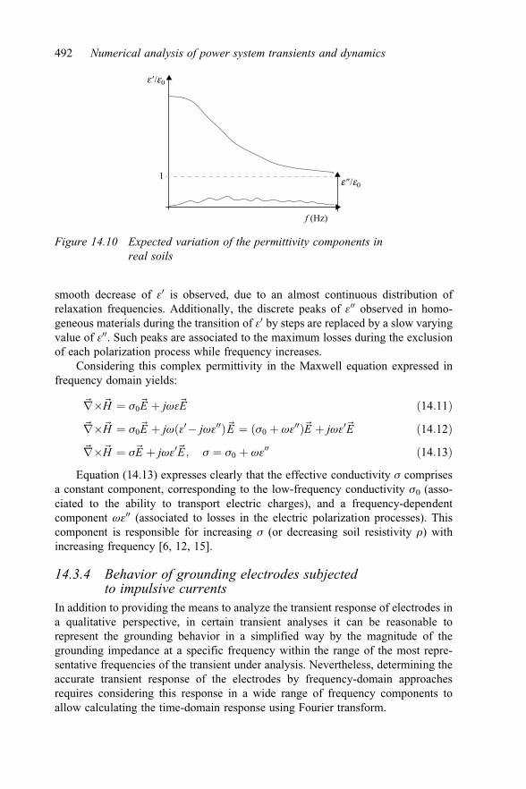
smooth decrease of e0 is observed, due to an almost continuous distribution ofrelaxation frequencies. Additionally, the discrete peaks of e00 observed in homo-geneous materials during the transition of e0 by steps are replaced by a slow varyingvalue of e00. Such peaks are associated to the maximum losses during the exclusionof each polarization process while frequency increases.

Considering this complex permittivity in the Maxwell equation expressed infrequency domain yields:

~r�~H ¼ s0~E þ jwe~E ð14:11Þ~r�~H ¼ s0~E þ jwðe0� jwe00Þ~E ¼ ðs0 þ we00Þ~E þ jwe0~E ð14:12Þ~r�~H ¼ s~E þ jwe0~E; s ¼ s0 þ we00 ð14:13Þ

Equation (14.13) expresses clearly that the effective conductivity s comprisesa constant component, corresponding to the low-frequency conductivity s0 (asso-ciated to the ability to transport electric charges), and a frequency-dependentcomponent we00 (associated to losses in the electric polarization processes). Thiscomponent is responsible for increasing s (or decreasing soil resistivity r) withincreasing frequency [6, 12, 15].

14.3.4 Behavior of grounding electrodes subjectedto impulsive currents

In addition to providing the means to analyze the transient response of electrodes ina qualitative perspective, in certain transient analyses it can be reasonable torepresent the grounding behavior in a simplified way by the magnitude of thegrounding impedance at a specific frequency within the range of the most repre-sentative frequencies of the transient under analysis. Nevertheless, determining theaccurate transient response of the electrodes by frequency-domain approachesrequires considering this response in a wide range of frequency components toallow calculating the time-domain response using Fourier transform.

f (Hz)

e″/e0

e ′/e0

1

Figure 14.10 Expected variation of the permittivity components inreal soils


Due to the large variety of transient occurrences in power systems, frequency-domain approaches associated with the application of Fourier transform consist ofa powerful tool to determine the transient response of electrodes. This varietymakes it very difficult to address the time response of grounding electrodes ingeneral approaches. Nevertheless, there is a class of relevant transient phenomena,consisting of impulsive currents and, notably, those related to lightning events,which it worths to address.

As mentioned, in general the primary response of electrodes subjected toimpulsive currents is expressed by the grounding potential rise GPR. The experi-mental results of Figure 14.11 illustrate this response for a grounding grid subjectedto the impression of impulsive currents with the same front time at the grid cornerand center [16–18].

Note the difference on the GPR curve according to the position of currentimpression on the grid.

In engineering applications, this response is commonly expressed in a simpli-fied way by means of the so-called impulse impedance ZP, defined as the ratiobetween the peak values of the grounding potential rise VP and impressed currentIP (14.14).

ZP ¼ VP=IP ð14:14ÞFigure 14.12 illustrates the concept of this impedance, referring to experi-

mental GPR curves obtained for a horizontal electrode subjected to differentimpulsive current waves [19].

Note that the waveforms of current and voltage are relatively similar in eachcase, though their peaks are not simultaneous due to reactive and propagationeffects in soil, notably for the wave with the shortest front time. Furthermore, quitedifferent values of ZP are found for the same grounding electrode buried in thesame soil, due to the different impressed current waves. This is explained by thedifference in the frequency content of the current waves in the high-frequencyrange, derived from the different front times. The wave with shortest front time,

00

5

10

15

20

25

30

1 2 3 4 5Time (μs)

(a) (b)

Vol

tage

(V)

Cur

rent

(A)

6 7 8 9 100

0.2

0.4

0.6

0.8

1

1.2

00

5

10

15

20

25

30

1 2 3 4 5Time (μs)

Vol

tage

(V)

Cur

rent

(A)

6 7 8 9 100

0.2

0.4

0.6

0.8

1

1.2

Measured GPRCurrent

Measured GPRCurrent

Figure 14.11 Measured GPRs of a 20 � 16-m grid, comprising 20 meshes of4 � 4 m, buried in a 2,000-Wm low-frequency resistivity soil andsubjected to impulsive 0.7-ms front-time currents: currentimpressed at the grid corner (a) and at the grid center (b)


whose superior frequency components have higher values, shows significantlylower impulse impedance (212 W), about the half-value of that of the long front-time wave (477 W). This is attributed to both the effect of significant capacitivecurrents flowing in this high-resistivity soil and the pronounced decrease of soilresistivity due to the frequency dependence effect. Nevertheless, in both cases thesame value of 1,536 W is obtained for the low-frequency resistance RT, as the ratio ofinstantaneous values of voltage v(t) and current i(t) at the wave tails [RT ¼ v(t)/i(t)].It is worth commenting that, though the impulse impedance is much lower than RT inboth cases, this result is specific for the condition of very high resistivity of soil andshort electrode. In low-resistivity soils, long electrodes commonly show the oppositeresult (ZP >> RT), as discussed in [17, 20].

In spite of the nonsimultaneous peaks of current and voltage, the impulseimpedance is very useful when expedite estimates of GPR are required for somedefined transient occurrences, such as in lightning protection applications. In thiscase, it is of interest to learn the grounding potential rise specifically for theimpression of representative current waves of first and subsequent return-strokes onelectrodes. Considering that ZP shows specific values for the first-stroke and for thesubsequent-stroke currents, their GPRs can be promptly obtained from the productof their assumed peak-current by the corresponding value of ZP [2, 4].

One fundamental aspect in the analysis of the response of grounding electrodesubjected to impulsive currents is the attenuation the current and voltage wavespropagating along the buried electrodes are subjected to. Because of attenuation,the current that is dispersed to the ground along the electrode presents a nonuniformdistribution, meaning that the linear current density (A/m) decreases along theelectrode. While the current and voltage waves propagates, the loss of energymainly associated with the electric field in the soil yields attenuation of theiramplitude and also reduction of their front steepness, as illustrated in Figure 14.13.This last effect is derived from the more intense attenuation the higher frequencycomponents associated to the wave front, as discussed in section 14.3.2 [4].

00

32

64

96

128

160

5 10

IP IP i(t)

15 20 25Time (μs)

(a)

Vol

tage

(V)

Cur

rent

(A)

30 35 40 45 500

0.1

0.2

0.3

0.4

0.5

00

50

100

150

200

250

1 2 3 4 5Time (μs)

(b)

Vol

tage

(V)

Cur

rent

(A)

6 7 8 9 100

0.3

0.6

0.9

1.2

1.5

VP

ZP = VP

Measured GPRCurrent

Measured GPRCurrent

RT = v(t)i(t)

v(t)

Figure 14.12 Measured GPRs of a 6-m-long horizontal electrode buried 0.5 mdeep in a 6.9-kWm low-resistivity soil. Front time of currentwaves and calculated ZP: (a) 4 ms and 477 W and (b) 0.4 ms and212 W. RLF ¼ 1,536 W


The parameter used to quantify the attenuation in time-domain analysis is theEffective Length of Electrode LEF, the counterpart of the space constant in thefrequency-domain analysis. As discussed in [4, 21, 22], LEF corresponds to a lim-iting length. Increasing the electrode length further does not yield reduction of thegrounding impedance value, considering that for this length high-frequency com-ponents of current associated with the wave front are strongly attenuated and pre-sent negligible amplitude.

As commented in section 14.4.3, attenuation increases with soil conductivityand frequency rise, considering that both parameters are responsible for increasingground losses. Thus, the value of LEF depends on the front time of the impulsivecurrent, as this time defines the superior frequency content of the wave. Thedecrease of both, front time and soil resistivity, leads to shorter values of LEF [4].

With respect to grids, it is usual to refer to an effective area as an extension of theconcept of the effective length of electrodes. This specific issue is discussed in [16].

A very useful parameter in lightning protection application is the ImpulseCoefficient IC, given by the ratio of impulse impedance and the low-frequencyresistance (14.15).

IC ¼ ZP=RT ð14:15ÞFigure 14.14 depicts the typical profile of IC as a function of the electrode

length and denotes that this coefficient varies from a value below one for shortelectrodes to values higher than it for electrodes longer than LEF [14, 18].

I0m I20m

Attenuation

Slope

Figure 14.13 Attenuation of the impulsive current wave propagating along theelectrodes attributed to losses in the soil

(a) (b)

LEF

L(m)

ZP/RT

Ic

1.0

0.4 to 0.7

LEF

L(m)

ZP/RT

Ic

1.0

0.8 to 1.0

Figure 14.14 Typical profile of the impulse coefficient IC as a function ofelectrode length in a high (a) and a low (b) soil resistivity,considering typical lightning current waves


As discussed in [14, 23], the values below one for electrodes shorter than LEF

are attributed to the superimposed effect of capacitive currents in the soil and ofsoil-resistivity frequency dependence, both of which contribute to making ZP lowerthan RT. The lowest values of this ratio (from about 0.4 to 0.7) are found for veryshort electrodes buried in high-resistivity soils. As the electrode length increases,the impulse impedance and the low-frequency resistance tend to decrease. How-ever, for electrodes longer than LEF, while the low-frequency resistance con-tinuously decreases by increasing electrode length, the value of ZP remainsconstant, leading to increasing values of IC above one, as discussed in [23–26].Thus, long electrodes buried in low-resistivity soils tend to present values of IC

much higher than one when subjected to current waves with very short front time.One time-domain related effect which affects the transient response of con-

centrate grounding electrodes is soil ionization, as discussed in the next section.

14.3.5 The soil ionization effectVery large current density can be experienced at the electrode surface when con-centrate (short-length) electrodes are subjected to very intense currents, such aslightning currents. The corresponding electric field in the region close to the elec-trode surface can exceed a critical limit, above which an ionization process takesplace in the soil leading to electrical discharges in this medium. The so-calledcritical electric field E0 ranges from 0.2 to 1.7 MV/m, depending on soil resistivityand humidity [27, 28].

The overall effect of soil ionization is an equivalent increase of the electrodedissipation area and a consequent reduction of the impedance ZP [4, 29, 30], asillustrated in Figure 14.15.

The low-impulsive voltage (50 kV) applied to a short electrode buried in alow-resistivity soil yielded a current with a peak value about 2 A, correspondingto an impulse impedance of about 25 W. As the voltage was increased to 5 kV(100-fold times), ionization process took place and current was increased to about410 A (almost 200-fold times), leading the impedance to decrease to about thehalf-value.

Two main complexities are involved when this nonlinear effect is taken intoaccount: defining the critical electric-field value, corresponding to the onset of theionization process, and considering the nonlinear distribution of the effect along the

0 1 2 3 4 5 6 7 8 9 100123456

010203040 Voltage

Current

50Vp

Ip

60

Time (μs)

Vol

tage

(V)

Cur

rent

(A)

0 1 2 3 4 5 6 7 8 9 100100200300400500600

01234

Voltage

Current

5Vp

Ip

6

Time (μs)

Vol

tage

(kV

)

Cur

rent

(A)

Figure 14.15 The effect of soil ionization


electrode due to propagation effects (attenuation of dispersed current along theelectrode).

Nevertheless, the dynamics of soil ionization have already been modeledby different approaches [31–34] and certain references recommend a value of400 kV/m for E0 [34], though values varying from 200 kV/m to more than1,000 kV/m have been reported in technical literature [27, 28, 35].

According to certain approaches, when the electric-field configuration is notsubstantially disturbed near the electrode by ionization process, assuming a givenvalue for E0, it is possible to consider this effect by means of an equivalent increaseof the electrode transversal section, allowing this increase to vary along the elec-trode length [32, 33]. This allows estimating the impact of the effect in the elec-trode response. However, for very concentrate electrodes, in which the effect ismore relevant, the ionized channels may entirely alter the field configuration,making it difficult to estimate this impact.

It is reasonable to ponder that the ionization effect is important for concentrateelectrodes, typically used in low-resistivity soils, from which low impedance valuesare obtained easily. In high-resistivity soils, long electrodes are usually required toensure low grounding impedance values. Thus, their current density tends to below, reducing the probability of soil ionization occurrence. In applications invol-ving long electrodes, such as the common counterpoises of transmission lines,neglecting the favorable effect of soil ionization is considered prudent [4, 36].

14.4 Numerical simulation of the transient responseof grounding electrodes

14.4.1 Preliminary considerationsThis section presents a set of numerical results intended to allow establishingquantitative references in relation to the concepts described in previous sections.The evaluations focused on typical electrode arrangements of high-voltage trans-mission lines in order to articulate the results of this section with the developmentsof the next section about the impact of the transient behavior of grounding elec-trodes on the lightning response of transmission lines.

All computational simulations were carried out using the Hybrid Electro-magnetic Model (HEM). This rigorous full-wave frequency-domain electro-magnetic model uses fast Fourier transform to convert the results to time domain. Itis called hybrid because, in spite of being formulated by means of electric fieldintegral equations, it provides results in terms of circuital quantities (voltages andcurrents) that are more useful in engineering applications [37].

In the application of this model, the simulated system is partitioned into nelements of different length, usually about 400 to 1,000 elements, depending on thecase. The model uses full n � n matrices expressing the electromagnetic couplingamong such elements to yield results. Preprocessing is used to determine thenumber of frequencies and of elements required to ensure quality to the simulatedresults. In regular applications, about 400 to 500 frequencies are processed in


each simulated condition (usual upper limit of 5 MHz for lightning-related pro-blems and a maximum frequency step of 12.5 kHz). Fast Fourier transform is usedto obtain results in time domain. It takes a few hours to process a complex simu-lated condition in regular personal computers. Details on the model formulation arefound in [37].

Specific applications of the model related to the lightning response of elec-trodes and lightning response of lines hit by direct strikes can be found in [13–16]and in [38–40], respectively. In particular, the use of the HEM model to calculategrounding potential rise and lightning overvoltage experienced across insulatorstrings of transmission lines was validated by comparing simulated and measuredresults, respectively in [12, 16] and [18].

The representative current waves of first and subsequent return-strokes ofFigure 14.16 were used in simulations. As discussed in [41–44], waveforms of first-return-stroke currents include an initial concavity followed by an abrupt rise aroundthe half-peak value and several subsidiary peaks, with the second peak usuallyturning out to be the highest one. On the other hand, the waveform of mostsubsequent stroke currents presents a single peak and a relatively smooth shape.The waves of Figure 14.16 [45] reproduces such patterns and also the medianparameters of currents measured at Morro do Cachimbo Station (MCS), in Brazil,comprising about 47 flashes and 138 subsequent stroke records [46, 47].

Very similar waveforms and time parameters were found after processing therecords of Berger’s measurements [48, 49], though their median peak-currentvalues were significantly lower, about 50% and 30% higher, respectively, for cur-rents of first and subsequent return-strokes. Table 14.1 indicates the parameters ofsuch currents.

In all simulations, frequency dependence of soil parameters was taken intoaccount by means of the Visacro-Alipio expressions (14.8) and (14.9). Soil ionizationwas disregarded, since in practical conditions of transmission-line tower-footings the

(a) (b)

0102030405060

0 10 20 30 40 50 60

Cur

rent

(kA

)

Time (µs)

0

5

10

15

20

0 2 4 6 8 10 12 14 16

Cur

rent

(kA

)

Time (µs)

Figure 14.16 Representation of typical waveforms of (a) first- and (b) subsequent-return-stroke currents with median parameters of currentsmeasured at MCS. The waveforms were reproduced using Heidlerfunctions, according to the procedures described in [41] and [45]for first- and subsequent-strokes


use of long electrodes results in low linear density of current dispersed along theelectrodes, decreasing the probability of occurrence of this effect.

The model was applied to determine the grounding potential rise experiencedat the electrodes due to the impression of the lightning current at the top of anisolated tower (all the current flows to the tower-footing electrodes), as denoted inFigure 14.17, which also represents the typical arrangement of transmission lineelectrodes consisting of counterpoise wires.

14.4.2 General results of the response of grounding electrodesGPR curves simulated for a 1,000-Wm low-frequency soil resistivity and corre-sponding impulse impedances of first and subsequent strokes are presented inFigure 14.18 to illustrate how the variation of the electrode length affects bothparameters.

Note that increasing the electrode length decreases the GPR peak, though thistrend is diminished as the length approaches LEF. This qualitative behavior is alsoobserved for soils of lower and higher resistivity, though in these cases thesaturation of the GPR decrease would occur, respectively, for shorter or longerelectrode length, according to the value of LEF for that resistivity. Also, it is clearthat, though the decrease of GPR peak is saturated with increasing electrode length,this increase still reduces the GPR values at the wave tail, whose amplitude isgoverned by the low-frequency resistance.

In addition to provide means to estimate the impulse impedance for specificconditions of soil resistivity and electrode length, ZP curves similar to those ofFigure 14.18(c) and 14.18(d) allow determining the effective length of the elec-trodes. LEF can be identified by inspection as the length in which the flat region,corresponding to the saturation of the impedance decrease with increasing electrodelength, begins. As discussed in [25], the effective lengths LEF of horizontal electro-des for currents of first and subsequent return-strokes are respectively about 13, 23,35, 48, 80 m and 8, 12, 18, 23, 36 m for soils of low-frequency resistivity of 100, 300,600, 1,000 and 2,000 Wm, considering frequency-dependent soil parameters.

Knowledge of the low-frequency grounding resistance of the tower-footingelectrodes is very useful, as measuring tower-footing impedance in field conditionsis a very difficult task for engineering personnel. Usually grounding resistance is

Table 14.1 Median parameters of lightning currents measured at MCSstation [46]

Event IP1 (kA) IP2 (kA) T10 (ms) T30 (ms) T50 (ms) dI/dt MAX (kA/ms)

FIRST 40.3 45.3 5.6 2.9 53.5 19.4SUB 16.3 – 0.7 0.4 16.4 29.9

Ip1 and Ip2 refer to the first and second return-stroke current peak value, T10 and T30 correspond,respectively, to the time between 0.1 Ip1 and 0.9 Ip1 and between 0.3 Ip1 and 0.9 Ip1, T50 is the timeinterval required for the current to decay to 0.5 Ip2, and dI/dtMAX is the maximum time derivative.


L

20 m6 m

6 m

Figure 14.17 Representation of the simulated condition to determine the GPR andof the grounding electrode arrangements. The 0.5-cm radiuselectrodes are buried 0.6 m deep in the soil. Their lengths L varyaccording to soil resistivity. The buried metallic parts of the towerwere represented by 3-m-long cylindrical vertical rods with10-cm diameter

00

200

400

600

800

1,000

5 10 15

L = 80 m

L = 60 mL = 40 m

L = 20 m

L = 80 mL = 40 m

L = 20 m

L = 10 m

20Time (μs)

(a)

Vol

tage

(kV

)

0 10 20 30 40 50 60 70 80 900

3530252015105

L (m)(c)

Z P (Ω

)

0 10 20 30 40 50 60 70 80 900

30252015105

L (m)(d)

Z P (Ω

)

00

10050

150

250200

350300

400

42 6 8 10 12Time (μs)

(b)

Vol

tage

(kV

)

Figure 14.18 Grounding potential rise of electrodes as a function of electrodelength for a 1,000-Wm soil, developed in response to the impressionof currents of (a) first and (b) subsequent return-stroke currents andcorresponding impulse impedances (c) and (d)


measured instead and the impedance is estimated according to the electrode con-figuration and soil resistivity. In this respect, it is very interesting to learn theimpulse coefficient IC of such configurations to allow prompt calculation of ZP

from the measured low-frequency resistance. Figure 14.19 depicts this coefficientspecifically for the conditions of Figure 14.18.

In the design of transmission lines, the requirements to achieve reasonablelightning performance lead to adopting different lengths of electrodes, as explainedin the next section. Longer electrodes are used in soils of higher resistivity to ensurethat the grounding impedance will not to exceed predetermined limits. Table 14.2indicates typical lengths of counterpoise wires used in real 138 kV lines for a set ofsoil-resistivity values.

14.4.3 Grounding potential rise of electrodes subject tolightning currents

The simulated GPRs developed in response to the impression of representativecurrents waves of first and subsequent strokes to the top of the 138 kV line, whosecounterpoise wires’ lengths are indicated in Table 14.1, are shown in Figure 14.20.

00

0.5

1

1.5

2

10 20 30 40 50L (m)

First strokesL (m)

20 20.5 24.3 0.8 10 24.8 37.1 0.720 15.6 24.3 0.740 11.2 14.9 0.880 11.1 8.8 1.3

40 12.1 14.9 0.860 8.8 11 0.880 7.6 8.8 0.9

ZP (W) RT (W) L (m) ZP (W) RT (W) IC = ZP /RTIC = ZP /RT

Subsequent strokes

I C60 70 80

FST

SUB

90

Figure 14.19 Calculated impulse coefficient for first (FST) and subsequent (SUB)strokes as a function of electrode length for the conditions ofFigure 14.18 (low-frequency soil resistivity of 1,000 Wm)

Table 14.2 Length of electrodes used for each soil resistivity

r0 (Wm) 100 600 1,000 2,000L (m) 5 30 50 70


14.4.4 Impulse impedance and impulse coefficient for firstand subsequent return-stroke currents

From the GPR curves in Figure 14.20 and the corresponding impressed currents,the impulse impedance was calculated, along with the low-frequency resistance andthe impulse coefficient (Table 14.3).

Note that the grounding-impedance increase due to the higher soil-resistivityvalues was partially offset by increasing the electrode length. While soil resistivityincreased 20-fold times, resistance increased by only about 400% and groundingimpedance by about 300% and 400%, respectively, for first and subsequent strokecurrents. Though increasing further the electrode length would lead to additionaldecrease of the grounding resistance, the impedance would show small variation,since the lengths of electrodes are relatively close to the effective length. Asexpected, in all cases the impulse coefficient is lower than one, as L is alwaysshorter than LEF.

00

100200300400500600700800

5 10Time (μs)

r0 = 100 Ω.m - L = 5 m

r0 = 600 Ω.m - L = 30 m

r0 = 2,000 Ω.m - L = 70 m

(a)

Vol

tage

(kV

)

15 20 00

50

100

150

200

250

5 10Time (μs)

r0 = 600 Ω.m - L = 30 m

r0 = 100 Ω.m - L = 5 m

r0 = 2,000 Ω.m - L = 70 m

(b)

Vol

tage

(kV

)

15 20

r0 = 1,000 Ω.m - L = 50 m

r0 = 1,000 Ω.m - L = 50 m

Figure 14.20 Simulated GPR of the 138-kV-line tower footing consideringdifferent values of soil resistivity r0: (a) first stroke and (b)subsequent stroke

Table 14.3 Calculated impulse impedance, resistance, and impulse coefficient ofelectrodes (curves of Figure 14.20)

r0 (W m) L (m) RT (W) First stroke Subsequentstroke

ZP (W) IC ZP (W) IC

100 5 5.1 4.6 0.9 3.7 0.73600 30 11.0 9.3 0.85 9.1 0.831,000 50 12.5 10.1 0.81 11.6 0.932,000 70 19.5 14.7 0.75 15.0 0.78


14.5 Case example: analysis of the influence ofgrounding electrodes on the lightning responseof transmission lines

Lightning is a frequent cause of transmission line outages. Though shielding fail-ures leading to lightning strikes to the phase conductors can contribute to a numberof faults, the backflashover largely prevails as the main cause of line outages, asdiscussed in [39, 50, 51]. This is the reason this mechanism, mainly governed bythe value of tower-footing grounding impedance, is the main focus of techniquesintended to improve the lightning performance of transmission lines.

Backflashover can occur due to direct lightning strikes to the towers or toshield wires at the towers’ vicinities, causing high overvoltages and, eventually,electrical discharges across insulators. The occurrence of such discharges dependson a balance between the insulator withstand and the amplitude of the lightningovervoltage the insulators experience in response to the injection of lightning cur-rents into the soil through tower-footing electrodes. Thus, decreasing tower-footinggrounding impedance is a very effective means to reduce this overvoltage and, inturn, to decrease backflashover occurrences. Figure 14.21 illustrates the effective-ness of this practice to reduce lightning overvoltage, based on the simulation of alightning strike to the top of an isolated tower of a 138 kV line, using the HEMmodel and the representative current of a first return-stroke of Figure 14.16(a).

Note that the increase of the tower-footing impedance (and, accordingly,the grounding resistance) from 20.5 to 7.6 W (resulting from increasing L from 20to 80 m) yielded a reduction of only about 15% of the overvoltage experiencedacross the upper insulator string. However, the reduction was much more sig-nificant at the wave tail.

00

Vol

tage

(kV

)

5 10Time (μs)

ZP = 20.5 Ω; RLF = 24.3 Ω

ZP = 12.1 Ω; RLF = 14.9 Ω

15 20

100200300400500600700

ZP = 7.6 Ω; RLF = 8.8 Ω

Figure 14.21 Simulated lightning overvoltage across the upper insulator string ofa real 138-kV line due to a strike to the top of a 30-m-high isolatedtower. Impressed first-stroke current of Figure 14.16(a). L ¼ 20, 40,and 80 m. Soil resistivity: 1,000 Wm


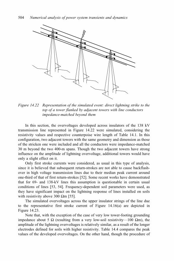
In this section, the overvoltages developed across insulators of the 138 kVtransmission line represented in Figure 14.22 were simulated, considering theresistivity values and respective counterpoise wire length of Table 14.1. In thisconfiguration, two adjacent towers with the same geometry and dimension as thoseof the stricken one were included and all the conductors were impedance-matched30 m beyond the two 400-m spans. Though the two adjacent towers have stronginfluence on the amplitude of lightning overvoltage, additional towers would haveonly a slight effect on it.

Only first stroke currents were considered, as usual in this type of analysis,since it is believed that subsequent return-strokes are not able to cause backflash-over in high voltage transmission lines due to their median peak current aroundone-third of that of first return-strokes [52]. Some recent works have demonstratedthat for 69- and 138-kV lines this assumption is questionable in certain usualconditions of lines [53, 54]. Frequency-dependent soil parameters were used, asthey have significant impact on the lightning response of lines installed on soilswith resistivity above 300 Wm [55].

The simulated overvoltages across the upper insulator strings of the line dueto the representative first stroke current of Figure 14.16(a) are depicted inFigure 14.23.

Note that, with the exception of the case of very low tower-footing groundingimpedance about 5 W (resulting from a very low-soil resistivity—100 Wm), theamplitude of the lightning overvoltages is relatively similar, as a result of the longerelectrodes defined for soils with higher resistivity. Table 14.4 compares the peakvalues of the developed overvoltages. On the other hand, though the procedure of

Figure 14.22 Representation of the simulated event: direct lightning strike to thetop of a tower flanked by adjacent towers with line conductorsimpedance-matched beyond them


increasing the electrode length is effective to reduce the impulse impedance, theamplitude of the overvoltage in the wave tail is still even higher for soilswith higher resistivity values. This occurs because in these conditions, the low-frequency tower-footing resistance is still even larger than those of lower resistivitysoils, as shown in Table 14.3. This resistance greatly influences the amplitude ofthe overvoltage at the wave tail.

The occurrence of flashover across insulators does not depend only on theovervoltage peak value but also on the whole overvoltage wave amplitude.

00 5 10

Time (μs)(a)

15 20

100Vol

tage

(kV

)

200300400500600

00 5 10

Time (μs)(c)

15 20

100Vol

tage

(kV

)

200300400500600

00 5 10

Time (μs)(d)

15 20

100Vol

tage

(kV

)200300400500600700

00 5 10

Time (μs)(b)

15 20

100Vol

tage

(kV

)

200300400500600

Figure 14.23 Voltage developed across upper insulator string of 30-m-high towerof the 138-kV line. (First stroke—MCS). Frequency-dependent soilparameters of resistivity r0 of 100 (a), 600 (b), 1,000 (c), and2,000 Wm (d). Two adjacent towers included (400-m span length)

Table 14.4 Peak of the overvoltage VP developed acrossthe upper insulator string of the 138-kV linefor the conditions of Figure 14.22

r0 (Wm) L (m) VP (kV)

100 5 424600 30 5211,000 50 5422,000 70 597


The literature presents several methods to assess flashover occurrence, such asthe v-x-t curves, the Disruptive Effect Model (DE) and the Leader ProgressionModel [56–59].

The DE, described in details in [57, 58], is considered a very consistent modeland was used in this chapter to assess the backflashover occurrence. Under a verysimplified approach, and considering specifically the evaluations developed in thissection, in this method a function of the instantaneous value of the differencebetween the overvoltage and a threshold voltage [v(t) � V0]1.36 is integrated in thetime interval, in which this threshold is exceeded. The constant V0 is given by aparcel of the line critical flashover overvoltage CFO (0.77�CFO). The occurrence ofbackflashover requires the result of this integration to be larger than a referencevalue DEb, which is given by DEb ¼ 1.15�CFO1.36.

It is worth mentioning that the literature reports the possibility to use differentvalues for the exponents and for the threshold in the expressions above to performthis evaluation, as discussed in [58, 59].

This method was applied to determine the minimum first-stroke peak currentrequired to achieve the backflashover occurrence in each of the conditions con-sidered in Figure 14.23 and assuming a line CFO of 650 kV, which is a typicalvalue for 138 kV lines. Table 14.5 shows the values calculated for this peak-current, known as critical current ICrit.

Note that all first-stroke currents of lightning strikes to the tower, whose peakcurrent were higher than ICrit would lead the line to a backflashover [60].

In spite of the longer electrode length with increasing soil resistivity, the cri-tical currents in higher resistivity soil show lower value, meaning that the prob-ability of backflashover has increased. The last column of Table 14.4 shows thepercentage of first-stroke lightning currents exceeding the critical peak currentaccording to the cumulative distribution of first-stroke peak-currents determinedfrom the currents measured at Morro do Cachimbo Station [61].

Note that, according to Table 14.5, the lightning performance of most towers isvery poor: about 23% and 43% of the strikes to the tower would lead to back-flashover and probably to line outage for the 1,000 and 2,000 Wm soils, respectively.

A rehearsal of the lightning performance of the line was developed, in terms ofits expected outage rates under certain conditions. The line was supposed tobe crossing a region with relative intense lightning activity, leading to an expectednumber of 20 flashes striking the line per 100 km per year. Assuming, as

Table 14.5 Critical first return-stroke peak-currents for the138-kV line CFO: 650 kV

r0 (Wm) L (m) ICrit (kA) IP > ICrit (%)

100 5 101 4600 30 67 191,000 50 63 232,000 70 49 43


recommended in [54], that only 60% of the flashes would strike to the towers or tothe shield wire in their vicinities, with potential to cause backflashovers, theexpected outage rates of the line were calculated considering the distributions ofsoil resistivity along the line shown in Table 14.6.

With the exception of the low-resistivity soil (100 Wm), in all cases of uniformdistribution of soil resistivity along the line the estimated outage rates are relativelyhigh, exceeding a rate of 2 outages/100 km/year. This rate is considered anacceptable limit for 138 kV lines in certain countries.

This low lightning performance of the towers installed on higher resistivitysoils results from the high values of the grounding impedances of their tower-footing electrodes. Moreover, one has to recognize also the very severe conditionsdetermined by the peak current distribution of MCS used in the calculations, as themedian peak current (45 kA) is about 50% higher than that of Berger’s distribution.Therefore, only for one of three assumptions of nonuniform distributions of soilresistivity along the line, the outage rate was lower than this threshold.

Anyway, this picture recommends working to improve the lightning perfor-mance of this line and this improvement could be achieved by reducing the tower-footing grounding impedances for the high-resistivity soils.

In order to demonstrate the impact of this impedance reduction, the lengths ofthe electrodes of towers installed on higher resistivity soils were increased, asindicated in Table 14.7. The results show that the increase of electrode lengths ledto lower first-stroke impulse impedance and larger critical currents. The same stepsdescribed previously in the rehearsal developed to obtain the data of Table 14.6were repeated. This resulted in lower lightning overvoltage amplitudes, decreasingthe backflashover outage rates of the line, as shown in Table 14.8.

Note that the calculated number of outage rates of the line decreased verysignificantly, achieving acceptable levels for the three usual nonuniform distribu-tions of soil resistivity along the lines, though this rate is still high specifically forthe 2,000-Wm soil resistivity.

Table 14.6 Expected outage rate of the 138-kV line (assumed: 20 strikes/100 km/year)

Hypotheses for the distribution of r (%) along the line Outages/100 km/year

100 WmL ¼ 5 m

600 WmL ¼ 30 m

1,000 WmL ¼ 50 m

2,000 WmL ¼ 70 m

100 0 0 0 0.440 100 0 0 2.20 0 100 0 2.70 0 0 100 5.120 40 30 0 1.815 35 35 15 2.60 40 30 20 2.7


The significant decrease of the outage rates derived from the increase in theelectrode length only (and, therefore, from the decrease in tower-footing impe-dance) demonstrates that this technique can be very effective to improve thelightning performance of transmission lines.

References

[1] Meliopoulos A. P. Power system grounding and transients. New York:Marsel Dekker Inc.; 1988.

[2] Visacro S. Low-frequency grounding resistance and lightning protection.Chapter 9: 475–502. Lightning protection. Cooray V. (Ed.), London: IET;2009.

[3] Visacro S. Grounding and earthing: Basic concepts, measurements andinstrumentation, grounding strategies. (in Portuguese). Sao Paulo: ArtLiberEdit.; 2002.

Table 14.7 Critical first return-stroke peak-currents for the 138-kVline CFO: 650 kV

r0 (Wm) L (m) VP (1st stroke)(kV) ICrit (kA) IP > ICrit (%)*

100 5 424 101 4600 40 498 [521] 77 [67] 11.6 [19]1,000 70 522 [542] 73 [63] 14.1 [23]2,000 100 575 [597] 60 [49] 26.1 [43]

*The value before increasing the electrode length is shown in brackets.

Table 14.8 Expected outage rate of the 138-kV line with longer electrodes(assumed 20 strikes/100 km/year)

Hypotheses for the distribution of r (%) along the line Outages/100 km/year*

100 WmL ¼ 5 m

600 WmL ¼ 40 m

1,000 WmL ¼ 70 m

2,000 WmL ¼ 100 m

100 0 0 0 0.440 100 0 0 1.4 [2.2]0 0 100 0 1.7 [2.7]0 0 0 100 3.1 [5.1]20 40 30 0 1.2 [1.8]15 35 35 15 1.6 [2.6]0 40 30 20 1.7 [2.7]

*The value in brackets corresponds to the outage rate before increasing the electrode length.


[4] Visacro S. ‘A comprehensive approach to the grounding response to light-ning currents’. IEEE Trans. Power Delivery. Jan 2007; 22: 381–386.

[5] Rudenberg R. ‘Fundamental considerations on grounding currents’. Elec-trical Engineering. Vol. 64, pp. 1–13, Jan 1945; 6 (1).

[6] Visacro S., Alipio R. ‘Frequency dependence of soil parameters: experi-mental results, predicting formula and influence on the lightning responseof grounding electrodes’. IEEE Trans. Power Delivery. Apr 2012; 27 (2):927–935.

[7] Heppe R. J. ‘Computation of potential at surface face above an energizedgrid or other electrode, allowing for non-uniform current distributions’.IEEE Trans. Power Delivery. 1998; 13: 762–767.

[8] Ramo S., Whinnery J. R., Duzer T. V. Fields and waves in communicationelectronics, New York: J. Wiley and Sons; 1965.

[9] Smith-Rose R. L. ‘The electrical properties of soils for alternating currents atradiofrequencies’. Proc. Royal Society. 1933; 140 (841A): 359–377.

[10] Scott J. H. Electrical and magnetic properties of rock and soil. U.S. Geol.Survey, Dept. of the Interior, Washington, 1966.

[11] Longmire C. L., Smith K. S. A universal impedance for soils. Topical Reportfor Period July 1–September 30, Defense Nuclear Agency, Santa Barbara,California, 1975.

[12] Visacro S., Portela C. M. ‘Soil permittivity and conductivity behavior onfrequency range of transient phenomena in electric power systems’. Int.Symp. High Voltage Engineering (ISH 1987), paper 93.06.

[13] Portela C. M. ‘Measurement and modeling of soil electromagnetic beha-vior’. IEEE Int. Symp. Electromagnetic Compatibility (IEEE EMC 1999):1004–1009.

[14] Visacro S., Alipio R., Murta Vale M. H., Pereira C. ‘The response ofgrounding electrodes to lightning currents: the effect of frequency-dependentsoil resistivity and permittivity’. IEEE Trans. Electromagnetic Compat-ibility. May 2011; 53 (2): 401–406.

[15] Alipio R., Visacro S. ‘Modeling the frequency dependence of electricalparameters of soil’. IEEE Trans. Electromagnetic Compatibility. 2014;doi:10.1109/TEMC.2014.2313977.

[16] Visacro S., Alipio R., Pereira C., Guimaraes M., Schroeder M. A. ‘Lightningresponse of grounding grids: Simulated and experimental results’. IEEE Trans.Electromagnetic Compatibility. 2014; doi 10.1109/TEMC.2014.2362091.

[17] Visacro S., Rosado G. ‘Response of grounding electrodes to impulsive cur-rents: an experimental evaluation’. IEEE Trans. Electromagnetic Compat-ibility. Feb 2009; 51: 161–164.

[18] Visacro S., Guimaraes M., Araujo L. ‘Experimental impulse response ofgrounding grids’. Electric Power Systems Research. 2013; 94: 92–98.doi.org/10.1016/j.epsr.2012.04.011.

[19] Rodrigues B. D., Visacro S. ‘Portable grounding impedance meter basedon DSP’. IEEE Trans. Instrumentation & Measurement. 2014; 10.1109/TIM.2014.2303532.


[20] Visacro S., Pinto W. L. F. ‘Is grounding impedance really larger thanlow frequency resistance?’ Conference Grounding and Earthing(GROUND’2006): 185–188.

[21] Gupta B. R., Thapar B. ‘Impulsive impedance of grounding grids’. IEEETrans. Power App. Syst. Nov/Dec 1980; PAS-99 (6): 2357–2362.

[22] Bewley L. V. ‘Theory and test of the counterpoise’. Electrical Engineering.Aug 1934; 1163–1172.

[23] Alıpio R., Visacro S. ‘Frequency dependence of soil parameters: Effect onthe lightning response of grounding electrodes’. IEEE Trans. Electro-magnetic Compatibility. 2013; 55: 132–139.

[24] Grcev L. ‘Impulse efficiency of ground electrodes’. IEEE Trans. PowerDelivery. Jan 2009; 24 (1): 441–451.

[25] Alıpio R., Visacro S. ‘Impulse efficiency of grounding electrodes: Effect offrequency-dependent soil parameters’. IEEE Trans. Power Delivery. 2014;29: 716–723.

[26] Grcev L. ‘Lightning surge efficiency of grounding grids’. IEEE Trans.Power Delivery. Jul 2011; 26 (3): 223–237.

[27] Oettle E. E. ‘A new general estimation curve for predicting the impulseimpedance of concentrated earth electrodes’. IEEE Trans. Power Delivery.1988; 3 (4): 2020–2029.

[28] Mousa A. M. ‘The soil ionization gradient associated with discharge of highcurrents into concentrated electrodes’. IEEE Trans. Power Delivery.Jul 1994; 9 (3): 1669–1677.

[29] Sekioka S., Sonoda T., Ametani A. ‘Experimental study of current-dependentgrounding resistance of rod electrode’. IEEE Trans. Power Delivery. Apr2005; 20 (2): 1579–1576.

[30] Geri A. ‘Behavior of grounding systems excited by high impulse currents:The model and its validation’. IEEE Trans. Power Delivery. Jul 1999; 14 (3):1008–1017.

[31] Liew A. C., Darveniza M. ‘Dynamic model of impulse characteristic ofconcentrated earths’. IEE Proc. Feb 1974; 121 (2): 123–135.

[32] Visacro S., Soares Jr. A. ‘Sensitivity analysis for the effect of lightningcurrent intensity on the behavior of earthing systems’. Int. ConferenceLightning Protection (ICLP 1994), paper R3a-01\(1-5).

[33] Almeida M. E., Correia de Barros M. T. ‘Accurate modelling of rod driventower footing’. IEEE Trans. Power Delivery. Jul 1996; 11 (3): 1606–1609.

[34] CIGRE C4.33.01 ‘Guide to procedures for estimating the lightning perfor-mance of transmission lines’. CIGRE Technical Brochure 63, Oct 1991.

[35] Lima J. L. C., Visacro S. ‘Experimental developments on soil ionization:New findings’. Int. Conference on Grounding and Earthing (GROUND2008): 174–179.

[36] Visacro S., Hermoso B., Almeida M. T., Torres H., Loboda M., Sekioka S.,Geri A., Chisholm W. ‘The response of grounding electrodes to lightningcurrents – summary report CIGRE WG C4.406’. Electra. 2009; 246: 18–21.


[37] Visacro S., Soares Jr. A. ‘HEM: A model for simulation of lightning-relatedengineering problems’. IEEE Trans. Power Delivery. Apr 2005; 20 (2):1026–1208.

[38] Soares Jr. A., Schroeder M. A. O., Visacro S. ‘Transient voltages in trans-mission lines caused by direct lightning strikes’. IEEE Trans. Power Deliv-ery. Apr 2005; 20 (2): 1447–1452.

[39] Visacro S., Silveira F. H., De Conti A. ‘The use of underbuilt wires toimprove the lightning performance of transmission lines’. IEEE Trans.Power Delivery. Jan 2012; 27 (1): 205–213.

[40] Silveira F. H., De Conti A., Visacro S. ‘Lightning overvoltage due to firststrokes considering a realistic current representation’. IEEE Trans. Electro-magnetic Compatibility. Nov 2010; 52 (4): 929–935.

[41] Visacro S. ‘A representative curve for lightning current waveshape of firstnegative stroke’. Geophysical Research Letters. Apr 2004; 31: L07112.

[42] Visacro S. Lightning: An engineering approach. (in Portuguese). Sao Paulo:ArtLiber Edit.; 2005.

[43] Visacro S., Vale M. H., Correa G., Teixeira A. ‘Early phase of lightningcurrents measured in a short tower associated with direct and nearby light-ning strikes’. Journal on Geophysical Research. 2010; 115 (D16104): 1–11.doi:10.1029/2010JD014097.

[44] Rakov V., Uman M. A. Lightning physics and effects. Cambridge: CambridgeUniversity Press; 2003.

[45] A. R. Conti, S. Visacro, ‘Analytical representation of single- and double-peaked lightning current waveforms’. IEEE Trans. Electromagnetic Com-patibility. 2007; 49: 448–451.

[46] Visacro S., Schroeder, M. A. O., Soares A. J., Cherchiglia L. C. L., Sousa V. J.‘Statistical analysis of lightning current parameters: Measurements at Morro doCachimbo Station’. Journal on Geophysical Research. 2004; 109 (D01105):1–11. doi:10.1029/2003JD003662.

[47] Visacro S., Mesquita C. R., De Conti A. R., Silveira F. H. ‘Updated statisticsof lightning currents measured at Morro do Cachimbo Station’. AtmosphericResearch. 2012; 117: 55–63.

[48] Berger K., Anderson R. B., Kroninger H. ‘Parameters of lightning flashes’.Electra. 1975; 41: 23–37.

[49] Anderson R. B., Eriksson A. J. ‘Lightning parameters for engineeringapplication’. Electra. 1980; 69: 65–102.

[50] Visacro S. ‘Direct strokes to transmission lines: Considerations on themechanism of overvoltage formation and their influence on the lightningperformance of lines’. Journal of Lightning Research. 2007; 1: 60–68.

[51] Brown G. W. ‘Lightning performance II – updating backflash calculations’.IEEE Trans. Power App. Syst. Jan/Feb 1978; PAS-97 (1): 39–52.

[52] IEEE PES Transmission and Distribution Com. ‘IEEE guide for improvingthe lightning performance of transmission lines’. IEEE Standard 1243, Dec1997.


[53] Silveira F. H., Visacro S., De Conti A. R. Lightning performance of 138-kVtransmission lines: The relevance of subsequent strokes’. IEEE Trans.Electromagnetic Compatibility. 2013; 55: 1195–1200.

[54] Silveira F. H., Visacro S., De Conti A., Mesquita C. R. ‘Backflashoversof transmission lines due to subsequent lightning strokes’. IEEE Trans.Electromagnetic Compatibility. Apr 2012; 54 (2): 316–322. doi:10.1109/TEMC.2011.2181851.

[55] Visacro S., Silveira F. H., Xavier S., Ferreira H. B. ‘Frequency dependenceof soil parameters: The influence on the lightning performance of trans-mission lines’. Int. Conference on Lightning Protection (ICLP 2012).

[56] Hagenguth J. H. ‘Volt-time areas of impulse spark-over’. AIEE Trans. 1941;60: 803–810.

[57] Hileman A. H. Insulation coordination for power systems. Boca Raton, FL:CRC Press; 1999.

[58] Darveniza M., Vlastos A. E. ‘The generalized integration method forpredicting impulse volt-time characteristics for non-standard wave shapes—A theoretical basis’. IEEE Trans. Electrical Insulation. Jun 1988; 23 (3):373–381.

[59] Chisholm W. A. ‘New challenges in lightning impulse flashover modeling ofair gaps and insulators’. IEEE Electrical Insulation Magazine. 2010; 26 (2):14–25.

[60] IEEE Working Group on Lightning Performance of Transmission Lines.‘A simplified method for estimating the lightning performance of transmis-sion lines’. IEEE Trans. Power App. Syst. Apr 1985; 104 (4): 919–932.

[61] Visacro S., Mesquita C. R., Dias R., Silveira F. H., De Conti A. ‘A classof hazardous subsequent lightning strokes in terms of insulation stress’.IEEE Trans. Electromagnetic Compatibility. Oct 2012; 54 (5): 1028–1033.doi:10.1109/TEMC.2012.2187339.


Index

admittance method formulation267–8

modified nodal analysis and 270–2airborne vehicles, lightning

electromagnetic environmentin 236

Ampere’s law 37, 214anemometer system 310–12

damaged 320wire diagram of 315–17

archorn: see protective gaparc modelling 84–5

Arc equations 85–6Thevenin-type component 86–8

ARENEanalysis conditions for 365and PSCAD/EMTDC 367–8

armature windings 12, 13A-stable 170, 171

integration method 176ATP Analyzer 77–8ATPDesigner 74–6ATPDraw 66–7

input dialogues 68line and cable modelling 68–70machine modelling 72–3main functionality 67–8MODELS module 73transformer modelling 70–2

automatic voltage regulator (AVR)of SVC 465

PI control function 466slope reactance control quantity,

function for adding 466voltage control quantity, function for

calculating 465–6

back flashover process 419–20back-flow surge 360

overhead earthing wire forprevention of 370

evaluation of possibility of SPD’sburning out 373–5

evaluation of potential rise ofearthing system 376–7

model of collection line in WPP371–2

observation of waveforms aroundSPDs 372–3

SPD’s burnout incidents due to 368surge propagations analysis in

WPP 368–9surge waveforms, detail analysis

on 369–70winter lightning and 361

backward differentiation formulas(BDFs) 177

backward Euler (BE) method 110,169–71, 174, 177, 270, 272

BCTRAN module 51, 70, 93, 98

C++ language 207center-to-center retardation

approximation 260–2Central Research Institute of Electric

Power Industry (CRIEPI)169

circuit-breaker (CB) 84circuit theory-based tool: see

electromagnetic transientsprogram (EMTP)

combined heat and power (CHP)systems 393

communications, security andmanagement of large systemstudies 153–4

complex grounding impedance 485conductor for cable constant

calculations 158constant-parameter distributed line

model (CPDL) 51, 60continuous operating voltage

(COV) 412controlled non-linearity 58control parameter settings survey 467–9control systems

MODELS 63, 65simulation of 114–16transient analysis of 63–4user-definable component 65–6

Cooray-Rubinstein formula 222Critical Damping Adjustment (CDA)

169, 170, 181, 186critical flashover overvoltage (CFO) 506current amplitude, influence of 82current diversion ratio method 383, 384current transformer (CT) saturation 381

Data Base Module 51dead time range 473digital fault locator algorithms 382diode switch 15discrete Fourier transform (DFT) 93,

94, 267discrete inverse Fourier transforms

(DIFTs) 267Disruptive Effect Model (DE) 506distributed-parameter circuit 181–4Dommel, H.W. 2DV-type AVR 435dynamic HTML (DHTML) 106

earthing systemevaluation of potential rise of 376–7in wind power plants 362–3of wind turbines 302, 307, 322

earth resistivity 322measuring point of 323

effective length of electrode 495

electric field integral equation (EFIE)272

electromagnetic field calculation byPEEC model 274–6

electromagnetic transients program(EMTP) 1, 103, 169–70, 381,445–6

application examples 122geomagnetic disturbances 128–30HVDC transmission 130–2IEEE-39 benchmark bus

example 124–6switching transient studies 122–4very large-scale systems 132wind generation 126–8

basic input data 24–7, 29circuit theory-based approach 1control systems 114–16equivalent resistive circuit 4–7external programming interface

121–2frequency-dependent line model 8–9implementation 120main modules of 103–4models 120–1multiphase load-flow solution and

initialization 116–18initialization from steady-state

solution 119–20initialization of load-flow

equations 119load-flow constraints 118–19

network equations for steady-state andtime-domain solutions 106–9

nodal analysis 2–4nonlinear models 111–12

state-space analysis 112–13steady-state solution 113time-domain solution 113

power system elements prepared in 24sparse matrix 7–8steady-state solution 109switches 13–18three-phase synchronous machine

10–11time-domain solution 109–11


transformer 9–10universal machine 11–13

embedded simulation modules TACSand MODELS 49–50

EMTDC (ElectroMagnetic Transientsfor DC) 135–8

capabilities of 138–9interpolation between time steps

139–41see also PSCAD/EMTDC

EMTP-ATP 47arc modelling 83–5

arc equations 85–6power system toolbox 93Thevenin-type component 86–8transformer inrush current

calculations 88–91capabilities 48

built-in electrical components 48embedded simulation modules

TACS and MODELS 49–50control systems 63

MODELS 65TACS 63–4user-definable component 65–6

frequency-domain analysis 52graphical preprocessor ATPDraw

66–7input dialogues 68line and cable modelling 68–70machine modelling 72–3main functionality 67–8MODELS module 73transformer modelling 70–2

lightning study 78current amplitude, influence of 82flashover model 80–1line model 78–80surge arrester model 81–2tower model 80voltage at substation 82

neutral coil tuning 82–3post- and pre-processors 73–4

ATP Analyzer 77–8ATPDesigner 74–6PlotXY program 74

power flow option 52–3solution methods 53

electrical machines 62–3non-linearities 58switches 53–8transmission lines 58–61

supporting modules 50–1typical power system studies 53

EMTP-RV 103energy absorption capability 414equivalent resistive circuit 4E-TRAN translator 138, 146

interfacing with 143E-TRAN substitution library 145formation of network

equivalents 143–4initialization of machines,

generators and sources 144–5European EMTP-ATP Users Group

(EEUG) 47excitations of lightning channel

220–1eXpandable Transient Analysis

Program: see XTAP(eXpandable TransientAnalysis Program)

external programming interface121–2

FACTS (Flexible AC TransmissionSystems) 431

category 431–2circuit configuration 432control system and simulation

modeling 433–4high-order harmonic resonance

phenomena 444considerations and

countermeasures 455–7correlation between impedance

and harmonic voltage 450electromagnetic transient program

(EMTP) analysis 445–6field test 453–4frequency–impedance ( f–Z)

characteristics of grid 446–50

Index 515

harmonics of a voltage-sourcedconverter 444–5

principle of 450–3STATCOM, application of 434

overvoltage suppression 442–3small-signal stability 436–7transient stability 441–2voltage fluctuation 435–6voltage stability 437–40

Faraday’s law 161, 216fast Fourier transform 267, 445, 497fast-front overvoltage 403, 406–7, 410fault locator 381

algorithms 382–3fault locator model description using

MODELS 383–5influence of fault arc characteristics,

study on 385–9finite-difference time-domain (FDTD)

method 41–2, 213, 291, 299,304–5, 314

advantages and disadvantages 217applications 221

lightning electromagneticenvironment in airbornevehicles 236

lightning electromagneticenvironment in powersubstation 236

lightning electromagnetic fields atclose and far distances 221–7

lightning surges andelectromagnetic environment inbuildings 238

lightning surges on overheadpower distribution lines 233–6

lightning surges on overheadpower transmission lines andtowers 227–33

surges on grounding electrodes238–9

configurations of 295excitations 220–1fundamentals 214–16lightning return-stroke channels

217–20

simulation model, investigations by350–4

simulations using 307finite-element method (FEM) 38, 213flashover model 80–1, 277

of archorn 282with nonlinear inductance 419

frequency-dependent line model 8–9frequency-domain analysis, in

EMTP-ATP 52frequency domain circuit equations and

solution 267admittance method formulation

267–8modified nodal analysis formulation

with stamp inspection 268–9frequency scan (FS) 52

gantry tower 417–18gap switch 14–15Gear-Shichman (GS) method 174,

176, 177Geoelectric Field (GEF) 128geomagnetic disturbances 128–30Gibb’s oscillation 267global gain margin 150Global Wind Energy Council

(GWEC) 359graphical user interface (GUI)

104–6, 207Green function for plane half space

259grounding, power system transients

and 481grounding electrodes, surges on 238–9grounding potential rise (GPR) 483,

489, 493, 499of electrodes subject to lightning

currents 501–2grounding resistance 407, 483, 499grounding systems 482–4

surge characteristics of 284–6grounding systems, transients

on 481numerical simulation of grounding

electrodes 497


electrodes subject to lightningcurrents, grounding potentialrise of 501–2

general results of response ofgrounding electrodes 499–501

impulse impedance and impulsecoefficient for return-strokecurrents 502

lightning response of transmissionlines, analysis of influence of503–8

preliminary considerations 497–9power system transients and

grounding 481response of grounding electrodes

subjected to transientscurrents 484

grounding electrodes and harmoniccurrents, behavior of 484–8

grounding electrodes behaviorsubjected to impulsivecurrents 492–6

soil ionization effect 496–7soil resistivity and permittivity,

frequency dependence of488–92

half-wave rectifier circuit 181, 183Harmonic Frequency Scan (HFS) 52,

152harmonic resonance phenomena,

high-order 444considerations and

countermeasures 455–7correlation between impedance and

harmonic voltage 450electromagnetic transient program

(EMTP) analysis 445–6field test 453–4

condition 453results 453–4

frequency–impedance ( f–Z)characteristics of grid 446–50

harmonics of voltage-sourcedconverter 444–5

principle of 450–3

HVDC transmission 130–2Hybrid Electromagnetic Model

(HEM) 213, 481, 497–8

IEC 62271-100 406IEEE-39 benchmark bus example

124–6impedance relay type method

382, 383impulse coefficient 495, 502impulse impedance 493, 502independent earthing 347, 348, 349insulation and semiconductive layers

permeability 159–60permittivity 158–9

insulation coordination study 408representative overvoltages,

determination of 408fast-front overvoltage 410slow-front overvoltage 410temporary overvoltage 409–10very-fast-front overvoltage 410

representative overvoltages, stepsfollowing the determination of410–12

study flow 408integrated earthing 347, 349, 354Interpolated Auto-Regressive Moving

Average (IARMA) convolutionmethod 61

inverse fast Fourier transform (IFFT)267

inverter circuit, actual 197–205IPFC (integrated power flow

controller) 432

JMarti Setup 51

Katzenelson algorithm 187, 188, 189,193–4, 202

Kirchhoff’s current law (KCL) 257Kirchhoff’s voltage law (KVL)

257, 258Kizilcay’s time-dependent model

386–9Kyushu Goto Island chain 461

Index 517

Leader Progression Model 506Leuven EMTP Center (LEC) 47lightning accidents and investigations

308measurements and simulations

of transient earthingcharacteristic 314–17

protection methodologies 312–14situations of accidents 310–12

lightning electromagnetic environmentin airborne vehicles 236in power substation 236

lightning electromagnetic fields atclose and far distances 221–7

lightning electromagnetic pulses(LEMPs) 213

lightning impulse protective level(LIPL) 413–14, 424

lightning impulse withstand voltage(LIWV) 411, 422

lightning protection systems (LPSs)359, 377

lightning response of transmission linesanalysis of influence of grounding

electrodes on 503–8lightning return-stroke channels

217–20lightning strike current 407, 418–19lightning study 78

current amplitude, influence of 82flashover model 80–1line model 78–80surge arrester model 81–2tower model 80voltage at substation 82

lightning surgesand electromagnetic environment in

buildings 238on overhead power distribution

lines 233–5on overhead power transmission

lines and towers 227–32lightning surges in renewable energy

system components 291solar power generation system 318

MW-class solar power generationsystem 319–39

overvoltage caused by lightningstrike 339–54

wind turbine 291earthing characteristics of a wind

turbine 300–8example of lightning accidents

and its investigations 308–17overvoltage caused by 291–300

linear, ordinary delay differentialequation (LODDE) system 272

linear capacitors, formula for 172–3linear inductors, formula for 172–3Line Constants 50–1line model 78–80

distributed-parameter 59–60lumped-element 58transmission line models 61, 278

load-flow constraints 118–19load-flow equations, initialization

of 119Lobatto III-C 272

magnetic permeability of soil 488MATLAB�/Simulink� 138

PSCAD/EMTDC interfacing to142–3

matrix formulation and solution 266frequency domain circuit equations

and the solution 267admittance method formulation

267–8modified nodal analysis

formulation with stampinspection 268–9

time-domain circuit equations andthe solution 269

modified nodal analysis andadmittance methodformulations 270–2

PEEC model order reduction 272time integration methods 270

maximum fitting error and propagationfunction 157–8


maximum order of fitting andpropagation function 157

maximum power point tracking(MPPT) control 198

Maxwell’s equations 37–8, 214measuring switch 16metallic screen 159, 160metal-oxide surge arresters 17, 18method of moments (MoM) 38,

213, 248in frequency domain 40in time domain 38

mixed-potential integral equation(MPIE) 247–8, 250–2

model order reduction (MOR)technique 270, 272

MODELS 22, 65, 381, 382, 400design objectives of 22–3fault locator model description

using 383–4implementation of 23–4

modified Fourier transform (MFT) 267modified iterative Fourier transform

(MIFT) 267modified nodal analysis (MNA)

method 257, 266–7and admittance method

formulations 270–2formulation with stamp inspection

268–9modified transmission-line model with

linear current decay model withlinear current decay (MTLL)model 220

modular multilevel converters(MMCs) 130

multiphase load-flow solution andinitialization 116–18

initialization from steady-statesolution 119–20

initialization of load-flowequations 119

load-flow constraints 118–19multiple control function

optimizations 150

MW-class solar power generationsystem 319

experiments using 1/10 scale model320–33

simulations in case of an actual-scalemodel 330–9

simulations using FDTD method of1/10 scale model experiments328–30

neutral coil tuning 82–3neutral delay differential equations

(NDDEs) 271Newton-Raphson (NR) algorithm 186

biaxial 191–2, 194standard 189, 194

nodal analysis 1–2, 4, 106, 266–7nominal discharge current 366, 413nonlinear elements 18–19, 277–8

compensation method 19current-source representation 19

non-linearities 58controlled 58Jiles–Atherton 91pseudo 58true 58

nonlinear models of EMTP 111–12state-space analysis 112–13steady-state solution 113time-domain solution 113

Norton equivalent 65–6, 112, 121numerical electromagnetic analysis

(NEA) 36–7, 38, 39Maxwell’s equations 37–8method of moments (MoM) 38see also finite-difference

time-domain (FDTD) methodNumerical Electromagnetics Code

(NEC-2) 279

object-oriented design of simulationcode 207–8

object-oriented methods, for powersystem simulations 207

object-oriented programming 207

Index 519

ordinary differential equations(ODEs) 206, 271

‘‘oscillation-free’’ integration method169, 170, 184

outer insulation 160–1overhead line model 79, 416overhead power distribution

lines, lightning surges on233–5

overhead power transmission lines andtowers, lightning surges on227–33

overvoltage 17, 349, 403caused by lightning strike 339–54caused by lightning surge

propagation on a windturbine 291

caused by potential rise 298–300classification of 403

fast-front overvoltage 406–7slow-front overvoltage 405–6temporary overvoltage 404–5very-fast-front overvoltage 407

insulation coordination study 408representative overvoltages,

determination of 408–10representative overvoltages, steps

following the determination of410–12

study flow 408steady-state 334, 342, 344suppression 442–3surge arresters, selection of 412

continuous operating voltage(COV) 412

energy absorption capability 414nominal discharge current 413protective levels 413–14rated short-circuit current 415rated voltage 413study flow 415

transient analysis, example of 416model setup 416–22results of the analysis 422–8

voltage shapes of 404

parallel damping resistors 273–4partial differential equations (PDEs) 2,

6, 206partial element calculation 262

excess capacitance 266partial inductance calculation 263–5partial potential coefficient

calculation 265–6partial resistance calculation 266

partial-element equivalent-circuit(PEEC) method 213, 247

application examples 277grounding systems, surge

characteristics of 284–6transmission towers, surge

characteristics of 277–83center-to-center retardation

approximation 260–2circuit interpretation of 257–8current element in 253current elements and potential

elements in 255derivation of 252–7discretization of PEEC elements

258–9discretization of structure in 252electromagnetic field calculation

by 274–6formulation of 252–60for plane half space 259–60matrix formulation and solution 266

frequency domain circuitequations and the solution267–9

time-domain circuit equations andthe solution 269–72

mixed potential integral equation(MPIE) 250–2

partial element calculation 262excess capacitance 266partial inductance calculation

263–5partial potential coefficient

calculation 265–6partial resistance calculation 266


procedures in the simulation of 249quasi-static PEEC models 262stability of 272

+PEEC formulation 273parallel damping resistors 273–4

+PEEC formulation 273phase-to-earth overvoltage 406, 411–13phase-to-phase fault 96, 392phase-to-phase overvoltage 406photovoltaic (PV) power generation

system 197photovoltaic power plants (PVPPs)

318–19, 321–3, 331, 334plane half space, PEEC models for

259–60PlotXY program 74post- and pre-processors 73–4

ATP Analyzer 77–8ATPDesigner 74–6PlotXY program 74

power conditioning systems (PCSs)319, 321–8

power flow option 52–3power oscillation damping (POD) 436,

441power substation, lightning

electromagnetic environmentin 236

power system circuits 171, 205power system elements 2, 3, 24power system stabilizer (PSS) 441power system studies, by EMTP-ATP

53power system toolbox 93

phasor calculations 93–6power and impedance calculations

96relay functionality 96result 97–9

PRIMA algorithm 272protective devices 381

fault locator 381algorithms 382–3fault locator model description

using MODELS 383–5

study on influence of fault arccharacteristics 385–9

high-speed switchgear 393comparative study with

measurement 395–7influence of voltage sag

magnitude 397–400modeling methods 395

study on influence of errors in inputdevices 389–94

surge 238, 317, 318protective gap 14, 17protective levels 413

lightning impulse 413, 414, 423–4switching impulse 413

PSCAD/EMTDC 135application to cable transients 154–5cable constant calculations,

parameters for 158cable model improvements 161–2conductor 158insulation and semiconductive

layerscommunications, security and

management 153–4capabilities of 138comparison analysis between

ARENE and 367–8exact modelling of power system

equipment 148hybrid simulation 146–8interfacing to MATLAB/Simulink

142–3interfacing with E-TRAN translator

143E-TRAN substitution library 145formation of network

equivalents 143–4initialization of machines,

generators and sources 144–5interpolation between time steps

139–41large and complex power system

models 148–9operations in 145–6

Index 521

parallel processing 152–3simulation set-up 155–6

curve-fitting starting and endfrequency 156–7

maximum fitting error andpropagation function 157–8

maximum order of fitting andpropagation function 157

total number of frequencyincrements 157

travel time interpolation 156specialty studies with 149–50

global gain margin 150harmonic frequency scan 152multiple control function

optimizations 150sub-synchronous control

interaction (SSCI) 151sub-synchronous resonance

(SSR) 150–1user-built modelling 141–2

pseudo-non-linearity 58PSS�E 138pulse width modulation (PWM)

control 444, 455PV module wirings 350

quasi-static PEEC models 262

rated short-circuit current 415rated voltage 413remote earth 483, 485representative overvoltages 403

determination of 408fast-front overvoltage 410slow-front overvoltage 410temporary overvoltage 409–10very-fast-front overvoltage 410

steps following the determinationof 410–12

return-stroke speed 218–19, 233robust and efficient iterative scheme,

solution by 184iterative methods 188

biaxial NR algorithm 191–2

Katzenelson algorithm 193–4standard NR algorithm 189–91

iterative scheme used in XTAP194–5

numerical examples 195actual inverter circuit 197–205voltage-current curves with cyclic

loci 195–7problem description 187–8

Runge-Kutta methods 171–2

SATURA 511/10 Scale model 320–8Semlyen Setup 51series RC circuit 177, 178, 179, 180series RL circuit 178, 181, 182, 186silicon-carbide (SiC) 198Schottky barrier diodes (SBDs) 198simulation code, of XTAP 207–8slope reactance 466, 468, 473, 478

parameters for 468, 469slow-front overvoltage 404–6, 410–11small-signal stability, STATCOM for

436–7soil ionization effect 284, 496–7soil resistivity 156, 284, 484

frequency dependence of 488–92solar array

of large-scale photovoltaic powerplant 328

lightning conductor on a structureof 329

solar power generation system 318MW-class solar power generation

system 319experiments using 1/10 scale

model 320–7simulations in case of an

actual-scale model 330–9simulations using FDTD method

of 1/10 scale modelexperiments 328–30

overvoltage caused by lightningstrike 339

discussions of overvoltage 349–50


investigations by experiments341–9

investigations by FDTDsimulations 350–4

sparse matrix 7square voltage method 385–6SSSC (static synchronous series

compensator) 431–2S-stability 1762-Stage Diagonally Implicit

Runge-Kutta (2S-DIRK)method 169

analytical accuracy comparisonswith other integration methods174–6

analytical stability and stiff-decaycomparisons with otherintegration methods 176–7

integration algorithm 170–2linear inductors and capacitors,

formulas for 172–3numerical comparisons with other

integration methods 177distributed-parameter circuit

181–4half-wave rectifier circuit 181output from control system 184series RC circuit 177–8series RL circuit 178–81

STATCOM (static synchronouscompensator), application of431, 434

overvoltage suppression 442–3small-signal stability 436transient stability 441–2voltage fluctuation 435–6voltage stability 437–40

state-space analysis 112–13Static Var Compensator (SVC)

application to cable systems 461applied control parameters 472

dead time range 473slope reactance 473time constant 473–4voltage control method 473

automatic voltage regulator (AVR)465

function for adding the slopereactance control quantity 466

function for calculating thevoltage control quantity 465–6

PI control function 466commissioning test, verification at

475–7control parameter settings survey

467–9output characteristics 464required control function for 463simulation results, comparison of

469–72transient analysis, verification by

473–5transient analysis model 466–7V-I characteristics of 463–4voltage variations in an island,

typical example of 461–3statistics and systematic switches 16steady-state initialization method 205–6steady-state solution 15–16, 109, 113,

119–20, 205–6sub-synchronous control interaction

(SSCI) 151sub-synchronous resonance (SSR)

150–1surge arrester model 18, 81–2surge arresters 16–18, 403, 407,

421–2, 423–7continuous operating voltage

(COV) 412energy absorption capability 414nominal discharge current 413protective levels 413–14rated short-circuit current 415rated voltage 413study flow 415

surge characteristicsof grounding systems 284–6of transmission towers 277–83

surge protection devices (SPDs) 360,361

Index 523

burnout incidents of, mechanism of368

analysis of surge propagations inWPP 368–9

detail analysis on surgewaveforms 369–70

model for 365–6possibility of burning out of 373–5waveforms around 372–3

surges on grounding electrodes 238–9SVG (static var generator) 431switches 13–18, 53–8

diode switch 15gap switch 14–15measuring switch 16protective gap 17statistics and systematic

switches 16surge arresters 17thyristor switch 16time-controlled switch 14

switchgear, high-speed 393comparative study with

measurement 395–7influence of voltage sag magnitude

397–400modeling methods 395

switching impulse protective level(SIPL) 411, 413

switching impulse withstand voltage(SIWV) 411

switching transient studies 122–4synchronous machine (SM) model 10,

12, 62

Taikoyama Wind Farm 308TCSC (thyristor-controlled series

capacitor) 431, 432temporary overvoltage 404–5,

409–10, 413–14themodified-augmented-nodal analysis

(MANA) 107, 109Thevenin equivalent 10, 12, 18–19,

58, 65, 86Thevenin-type component 86–8

thin-wire time-domain (TWTD) code40, 280

thin wire time-domain (TWTD)simulation 279

three-phase synchronous machine 10thyristor-controlled series capacitor

(TCSC) 151, 431–2thyristor switch 16, 21, 394, 432time constant 178, 392, 473time-controlled switch 14time-domain circuit equations and

solution 109–11, 113, 269, 272modified nodal analysis and

admittance methodformulations 270–2

PEEC model order reduction 272time integration methods 270

time integration methods 270total harmonic distortion (THD)

455, 457tower-footing impedance 499, 503,

508tower model 80, 416–17transformer 9transformer inrush current

calculations 88–91transformer model 91–3transient analysis 404–5, 416

model 466–7model setup 416

back flashover 419–20gantry 417–18lightning strike 418–19overhead line model 416substation 420–1surge arrester 421–2tower 416–17

results of the analysis 422–8verification by 473–5

transient analysis of control systems(TACS) 2, 20, 63–4, 382

devices in 64and electric networks 20–1sources in 63transfer functions in 64


transient stability problem, STATCOMfor 441–2

transmission-line (TL) model 220transmission-line-matrix (TLM)

method 213transmission lines in EMTP-ATP 58–61transmission matrix method (TLM) 38transmission towers, surge

characteristics of 277–83transverse electric (TE) mode 36transverse electromagnetic (TEM)

mode 1transverse magnetic (TM) mode 36trapezoidal (TR) method 170, 174–7,

181, 184traveling-current-source (TCS) model

220true-non-linearity 58

unified power flow controller(UPFC) 432

universal machine 11–12, 62user-built modelling 141–2user-definable component 65–6

very-fast-front overvoltage 403, 407,410

very large-scale systems 132V-I characteristics of SVC 463–4voltage at substation 82voltage control method 436, 463, 473voltage–current (V–I) relation of the

arrester 234voltage–current curves with cyclic

loci 195–7voltage fluctuation, control of 434–6voltage sag waveform 399–400voltage-sourced converter (VSC):

see FACTS (Flexible ACTransmission Systems)

voltage stability, STATCOM for437–40

Vref-type AVR 435–6VSC-BTB (voltage-sourced converter

back-to-back) 431–2

wind farm 152, 308, 316, 318, 359,363, 434

wind generation 126–8windings 12wind power plants (WPPs), collection

system inearthing system in 363effect of overhead earthing wire

to prevent back-flowsurge 370

evaluation of possibility of theSPD’s burning out 373–5

evaluation of potential rise ofearthing system 376–7

model of collection line in WPP371–2

observation of waveforms aroundSPDs 372–3

lightning surge analysis, WPPmodels for 363

comparison analysis betweenARENE and PSCAD/EMTDC367–8

surge protection device (SPD)365–6

winter lightning 365mechanism of SPD’s burnout

incidents due to back-flowsurge 368

analysis of surge propagations inWPP 368–9

detail analysis on surgewaveforms 369–70

wind turbines, earthing system of362–3

winter lightning and back-flowsurge 361

Windsyn module 72–3wind turbine (WT), lightning surges

in 291, 359earthing characteristics 300

experiments at actual windturbines 302–6

frequency characteristics 307–8measurement sites 301–2

Index 525

multifarious earthing systems302

simulations using FDTD method307

earthing system of 362–3lightning accidents and

investigations 308protection methodologies 312–14situations of accidents 310–12transient earthing characteristic

314–17overvoltage caused by 291

analytical conditions 294experimental conditions 292–4lightning surge propagation 294–8overvoltage caused by potential

rise 298–300reduced-size model of 292

winter lightning 359and back-flow surge 361model for 365

XFMR module 70–2XFORMER 9, 51XTAP (eXpandable Transient Analysis

Program) 1692S-DIRK method, numerical

integration by 169

2S-DIRK integration algorithm170–2

analytical accuracy comparisonswith other integration methods174–6

analytical stability and stiff-decaycomparisons with otherintegration methods 176–7

linear inductors and capacitors,formulas for 172–3

numerical comparisons withother integration methods177–84

flowchart of the iterative schemeused in 195

object-oriented design of simulationcode 207–8

robust and efficient iterative scheme,solution by 184

iterative methods 188–94iterative scheme used in XTAP

194–5numerical examples 195–205problem description 187–8

steady-state initialization method205–6

ZNO FITTER 51


Documents

Numerical Analysis of Power System Transients and Dynamics