ISS

N 0

249-

6399

ap por t de r ech er ch e

INSTITUT NATIONAL DE RECHERCHE EN INFORMATIQUE ET EN AUTOMATIQUE

Numerical analysis of junctions between thinshells, Part 1 : continuous problems

Michel Bernadou , Annie Cubier

N ˚ 2921

Juin 1996

THEME 4

Numerical analysis of junctions between thin shells,Part 1 : continuous problemsMichel Bernadou*, Annie Cubier**Th�eme 4 | Simulationet optimisationde syst�emes complexesProjet MODULEFRapport de recherche n� 2921 | Juin 1996 | 22 pagesAbstract: The junctions of beams, plates and shells are the basic components ofany industrial structural construction. The numerical simulation of such junctionsis a classical part of the commercial �nite element codes. On the other hand it seemsthat there are very few mathematical studies of such junctions. In this paper, wepropose a variational formulation of junctions between thin shells when the junctioncan be considered as an elastic or a rigid hinge. Then, we study the mathematicalproperties of these equations.Key-words: Thin shells. Elastic junction. Rigid junction. Equilibrium equa-tions. Variational formulations. (R�esum�e : tsvp)*Pole Universitaire L�eonard de Vinci**INRIA RocquencourtUnite de recherche INRIA Rocquencourt

Analyse num�erique de jonctions de coques minces,Partie 1 : Probl�emes continusR�esum�e : Les jonctions de poutres, plaques et coques sont �a la base de nom-breuses constructions. La simulation num�erique de telles jonctions peut etre traiterpar certains codes d'�el�ements �nis. Cependant, il y a tr�es peu d'analyse math�ema-tique de ce type de probl�emes. Dans cet article, nous proposons une formulationvariationnelle de jonctions de coques minces dans le cas o�u la charni�ere a un com-portement �elastique ou rigide. Nous �etudions alors les propri�et�es math�ematiques deces �equations.Mots-cl�e : Coques minces. Jonction �elastique. Jonction rigide. Equationsd'�equilibre. Formulations variationnelles.

Junctions between thin shells 31 IntroductionMany industrial constructions use, as basic components, elastic beams, platesand shells. The numerical simulation of such assemblages needs a good approxima-tion of each constitutive element as well as a good representation of their junctions.In engineering literature, there are many contributions on the best way to modelizeand, particularly, to compute such constructions.Thus, for the modelization of the mechanical engineering aspects, we refer forinstance the reader to the chapter 6 of Baker-Kovalevsky-Rish (1981) which is devo-ted to multishell structures, to xx 3.4 and 6.2 of Fl�ugge (1973) which are concernedwith polygonal domes and with di�erent kinds of junctions between cylinders andspherical caps or ends, and to xx 11.4 and 18.5 of Calladine (1983) for pressure-vessel junction problems. For �nite element methods, we can recommand Bathe(1982) and Bathe-Ho(1981) and the references of these works.By contrast there are very few mathematical studies in these directions. Never-theless we can mention the works by Aufranc (1989) and Ciarlet (1990) which aremainly concerned with the problem of the junction between three-dimensional andtwo-dimensional linearly elastic structures while Le Dret (1991) consider asymptoticdevelopments for junction between two plates.In this series of papers, we restrict our attention to the numerical analysis of thejunction between two shells. Our study follows the main lines of Bernadou-Fayolle-L�en�e (1989) and lies on the following assumptions :� elastic, homogeneous, isotropic material,� small deformations,� deformation through the thickness satis�es the usual assumptions of Koiter(1966),� the junction can be assimilated to a rigid or to an elastic hinge.The contents of the Part 1 of this paper can be outline as follows : Section 2discusses the mechanical modelling of the junction between thin shells in terms ofpartial di�erential equations. We start by recalling the general Koiter equations ;then, we introduce the modelization of the junction as an elastic or a rigid hinge andwe conclude by giving some examples. Section 3 gives the variational formulationsof these di�erent junctions and the corresponding existence results. It is also pro-ved that the solution of the elastic hinge problem converges to the solution of therigid hinge problem when the elastic sti�ness of the hinge becomes very large. Theapproximation by �nite element methods will be analyzed in Part 2 of this paper.RR n� 2921

4 Michel Bernadou , Annie Cubier2 Mechanical modellingIn this section, we brie y introduce the main notations and the basic equationsthat we subsequently use. We refer the reader to Koiter (1966) for more detailsconcerning the equilibrium equations for one shell ; for convenience, we record themain topics in Paragraph 2.1.2.1 Equilibrium equations for one shellLet be a bounded open subset in a plane E2, with a su�ciently smoothboundary @. Then the middle surface S of the shell is de�ned as the image of theset � by a mapping � : � � E2 ! E3;where E3 is the usual Euclidean space. Subsequently, we assume that � 2 (C3(�))3and that all points of S = �(�) are regular, i.e., the two vectors a� = �;�; � = 1; 2,are linearly independent for all points � = (�1; �2) 2 �. With the covariant basis(a�) of the tangent plane, we associate the contravariant basis (a�) which is de�nedthrough the relations a� �a� = ��� (no summation if � = �), where ��� is the Krone-cker's symbol. We also introduce the unit normal vector a3 = a1 � a2= j a1 � a2 jand we set a = det(a��); a�� = a� � a� .By using such local covariant and contravariant bases, the linear equilibriumequations can be written as (see Koiter (1966), equations (11.27) and (11.28)) :[n�� + 12b��m�� � 12b��m�� ] j� +b��m�� j� +p� = 0 in S; (2.1)�m�� j�� +b��n�� + p3 = 0 in S; (2.2)with the following boundary conditions (see Koiter (1966), equations (11.29) and(11.31)) : [n�� + 32b��m�� � 12b��m�� ]n� = N� + b��M� on @S; (2.3)�m�� j� n� � (m��n�t�);s = N3 � (M�t�);s on @S; (2.4)m��n�n� =M�n� on @S: (2.5)In these equations, we have adopted the following notations :n��; m�� = symmetric tensors of tangential stress resultants and stress couples,b��; b�� = covariant and mixed components of the second fundamental form ofthe middle surface S;(:) j�= covariant derivative with respect to ��,p = piai = external loads referred to the middle surface S, INRIA

Junctions between thin shells 5n = n�a� = outward unit normal vector to the boundary @S in thetangent plane. This normal vector in the tangent plane shouldnot be confused with the stress tensor; (2.6)t = a3 � n = t�a� = unit tangent vector to the boundary @S ; (2.7)N = N iai = external edge loads per unit length of the boundary @S, (2.8)M = M�a� � a3 = (Mnn+Mtt)� a3 =Mtn�Mnt = externaledge moment loads per unit length of the boundary @S, (2.9)ds = line element along the boundary @S.Now, by assuming that :i) the material of the shell is elastic, homogeneous and isotropic,ii) the strains are small everywhere in the shell,iii) the state of stress is approximatively plane and parallel to the middle surface,it is proved in Koiter (1966) thatn�� = eE���� ��; m�� = e312E�������; (2.10)where E���� = E2(1+�) [a��a�� + a��a�� + 2�1�� a��a��]; �� and ��� denote respec-tively the elastic moduli tensor for plane stresses, the middle surface strain tensorand the modi�ed change of curvature tensor.Finally, the expressions of the components �� and ��� associated with a displa-cement vector v = viai are given by ��(v) = 12(v�j� + v�j�)� b��v3; (2.11)���(v) = v3j�� + b��j�v� + 14b��(3v�j� � v�j�) + 14b��(3v�j� � v�j�): (2.12)Variational formulation : subsequently, we assume that the shell is clampedalong a part @S0 = �( 0) of its boundary, with meas( 0) > 0, and that it is loadedalong its complementary part @S1 = �( 1); 1 = @ � 0 of its boundary by adistributed force N and a distributed moment M . From the equations (2.1) toRR n� 2921

6 Michel Bernadou , Annie Cubier(2.5), (2.11) and (2.12), Green's formula allows to state the problem in the followingform : For given p 2 (L2())3; N 2 (L2(@1))3; M 2 (L2(@1))3;find u 2 V such that a(u; v) = `(v); 8 v 2 V 9>=>; (2.13)where : a(u; v) = Z eE����f ��(u) ��(v) + e212���(u)���(v)gpad�1d�2;`(v) = Z p � vpad�1d�2 + Z 1(N � v +M � (v))d ; (2.14)and V = fv 2 (H1())2 �H2() ; v j 0= 0; v3;� j 0= 0g;where v;� denotes the outward unit normal derivative to the boundary 0. Moreover,in (2.14) we have assumed that the boundary 1 is parameterized by � ! �� = g�(�),so that d = qa��(g�)0(g�)0d�: (2.15)Let us detail some more the expression (2.14) : we have used the in�nitesimalrotation vector whose expression as function of displacement v is given by (v) = "��(v3;� + b��v�)a� + 12"��v�j�a3; (2.16)with "�� = 1pae��; e�� = 0 1�1 0 ! : (2.17)From (2.6),(2.7), (2.9) and (2.16), (2.17), we obtainM � (v) = (t�Mt + n�Mn)(v3;� + b��v�); (2.18)so that(v) = Z p � vpad�1d�2 + Z 1 [N � v + (t�Mt + n�Mn)(v3;� + b��v�)]d :Theorem 2.1.1 (Bernadou-Ciarlet (1976), Bernadou-Ciarlet-Miara (1994)): Theproblem (2.13) has one and only one solution.INRIA

Junctions between thin shells 72.2 Junction between two thin shellsConsider two thin shells whose middle surfaces S and S� joint along a commonboundary �. Subsequently, we assume that these middle surfaces S and S� are theimages through bijections � and �� of two bounded open subsets and � of a planeE2 with su�ciently smooth boundaries @ and @� . Moreover, we assume that :i) The middle surface S is clamped along a part �0 of its boundary, with meas(�0) >0, joints with S� along �, and is loaded along � and along the complementarypart �1 of the boundary. Brie y, we have@S = �0 [ �1 [ �: (2.19)Corresponding to this decomposition, we get through the application (�)�1:@ = 0 [ 1 [ : (2.20)ii) The shell S� joints with S along � and is loaded along � and along the comple-mentary part ��1 of its boundary so that@S� = ��1 [ �; @� = �1 [ � ; (2.21)where � = (��)�1(�).All these considerations are illustrated by Figure 1.Remark 2.2.1 : The boundary conditions and the representations of shells S and S�are purely indicative and can be extended to more general situations. In particular,i) we could consider the case of a shell S� which is also clamped along a part ��0of its boundary ;ii) we could consider more junctions using the same ideas.Subsequently, as a general rule, we note (:) the quantities related to the shell Swhile (��) denotes the quantities related to the shell S�.Upon the boundaries @S and @S�, we de�ne two local direct orthonormal refe-rence systems (n; t;a3) and (n� ; t� ;a�3) which include as intrinsic vectors the outwardunit normal vectors (see (2.6)), the unit tangent vectors (see (2.7)) and the vectorsa3 et a�3.Remark 2.2.2 : In a previous paper related to junction between plates, Bernadou-Fayolle-L�en�e (1989) introduced the angle � = (n;n�)t with respect to the referencesystem (n; t;a3). This parameter � was constant ; for junctions between shells, wecan similarly introduce the angle � = (n;n�)tRR n� 2921

8 Michel Bernadou , Annie Cubierwith respect to the reference system (n; t;a3), but in general, this angle is nolonger constant.

0 �1 1 0 1�2 �e2e1e3 S �1 � S� ��1��� �1 �1�0 ��2� �1�0Fig. 1 : Junction between two shells and its representation.Whatever the behaviour of the hinge � is, the application of the action-reactionprinciple at any point of �, implies the transmission of the external e�orts, i.e.,N(P ) = N�(P ) and M(P ) =M�(P ); 8P 2 �: (2.22)Note that the relation M (P ) = M�(P ) in conjunction with (2.9) and its analogupon S� implies Mt(P ) =M�t� (P ) = 0; 8P 2 �; (2.23)as soon as n� n� 6= 0. Then (2.9) and (2.23) imply :M (P ) =M�(P ) = �Mnt; 8P 2 �: (2.24)Subsequently, we assume that relations (2.23) and (2.24) are still satis�ed whenn � n� = 0 (junction of class C1).Then, we examine two types of hinge behaviour : INRIA

Junctions between thin shells 9i) a rigid behaviour which insures the continuity of the displacements and ofthe tangential rotations along the hinge for all points P of �, i.e.,u(P ) = u�(P );( (u) � t)(P ) = ( �(u�) � t)(P ) = [(t � t�)( �(u�) � t�)](P ); 9>=>; (2.25)where (u) (resp. �(u�)) is de�ned by relation (2.16);ii) an elastic behaviour which only insures the continuity of the displacementsfor all points P of �, i.e.,u(P ) = u�(P );Mn(P ) = k[( (u)� �(u�)) � t](P ): 9>=>; (2.26)Thus the second equation of relation (2.25) is replaced by the requirement : thetangential component of the moment M (see (2.9)) is proportional to the jump ofthe tangential components of the rotations along the hinge �. The coe�cient k mea-sures the elastic sti�ness along the hinge ; it is positive and it should be determinedexperimentally.Remark 2.2.3 : Generally, the parameter k is dependent on the position along thehinge �.On the other hand, the rigid behaviour can be interpretated as the limit case of theelastic behaviour of the hinge when sti�ness coe�cient k becomes very large. Wecome back to this remark in Paragraph 3.3.2.3 The equations of the junction problemIn this paragraph we summarize the equations of the junction problem. By takinginto account the assumptions made in Paragraphs 2.1 and 2.2, these equations aregiven by :[n�� + 12b��m�� � 12b��m�� ] j� +b��m�� j� +p� = 0 in S;�m�� j�� +b��n�� + p3 = 0 in S; 9>=>; (2.27)[n��� + 12b���m��� � 12b���m��� ] j� +b���m��� j� +p�� = 0 in S� ;�m��� j�� +b���n��� + p3� = 0 in S� : 9>=>; (2.28)In relation (2.28), we note for simplicity (j�) the covariant derivatives with respectto ��� . The corresponding boundary conditions areu = 0; u3;n = 0 on �0; (2.29)RR n� 2921

10 Michel Bernadou , Annie Cubier8>>>>><>>>>>: [n�� + 32b��m�� � 12b��m�� ]n� = N� + b��M� on �1 [ �;�m�� j� n� � (m��n�t�);s = N3 � (M�t�);s on �1 [ �;m��n�n� =M�n� on �1 [ � ;8>>>>><>>>>>: [n��� + 32b���m��� � 12b���m��� ]n�� = N�� + b���M�� on ��1 [ �;�m��� j� n�� � (m��� n��t��);s� = N3� � (M�� t��);s� on ��1 [ �;m��� n��n�� =M�� n�� on ��1 [ � ;8><>: N(P ) = N�(P ); 8P 2 �;M(P ) = M� (P ) = �M n(P )t; 8P 2 �;while the conditions of junction upon � depend on the type of hinge :� rigid hinge ( see (2.16) and (2.25))u = u� on �; (u) � t = (t � t�) �(u�) � t� on � ; 9>=>; (2.30)� elastic hinge (see (2.16) and (2.26))u = u� on �;k[ (u) � t� (t � t�) �(u�) � t� ] =Mn on �: 9>=>; (2.31)2.4 Some examplesLet us consider three examples : two are extracted from practical engineering situa-tions and the third from a classical benchmark.Hyperbolic paraboloid roof for Hamburg Sechslingspforte swimming poolAs a �rst example, let us recall that mentionned by Argyris-Lochner (1972) andLeonhardt-Schlaich (1970). The roof consists of two identical straight-edged shellsABCD and A0C0BD (see Figure 2) which joint along the edge BD and which aresymmetrical with respect to this edge. The middle surface of each shell has theform of a hyperbolic paraboloid with straight edges. Of course, in the real lifesituations, the structure is much more complicated since it includes sti�eners andother appliances.Junction between two cylindrical tubesO�shore plateforms (see for example Alencar-Ferrante (1984)) are built by as-sembling a large number of tubular joints. The junction of two cylindrical tubesconstitutes the basic node of such a structure (see Figures 3 and 4). INRIA

Junctions between thin shells 11

Fig. 2: Geometry of the hyperbolic paraboloidal shells.Main tubeY 2 + Z2 = R2 , � = 8><>: X = XY = R cos �Z = R sin �Secondary tube�� = 8><>: X = C + u cos� � r sin � cos�Y = u sin � + r cos � cos�Z = r sin �Fig. 3 : Intersection lines.RR n� 2921

12 Michel Bernadou , Annie Cubier

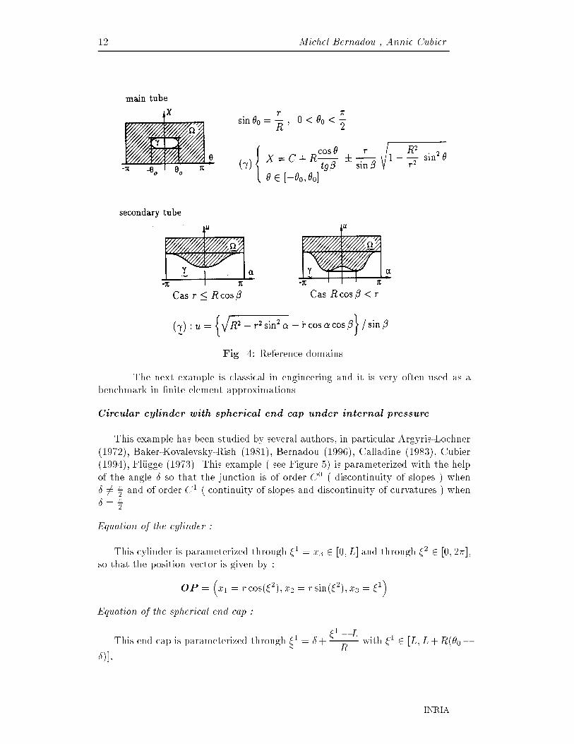
Fig. 4: Reference domains.The next example is classical in engineering and it is very often used as abenchmark in �nite element approximations.Circular cylinder with spherical end cap under internal pressureThis example has been studied by several authors, in particular Argyris-Lochner(1972), Baker-Kovalevsky-Rish (1981), Bernadou (1996), Calladine (1983), Cubier(1994), Fl�ugge (1973). This example ( see Figure 5) is parameterized with the helpof the angle � so that the junction is of order C0 ( discontinuity of slopes ) when� 6= �2 and of order C1 ( continuity of slopes and discontinuity of curvatures ) when� = �2 .Equation of the cylinder :This cylinder is parameterized through �1 = x3 2 [0; L] and through �2 2 [0; 2�],so that the position vector is given by :OP = �x1 = r cos(�2); x2 = r sin(�2); x3 = �1�Equation of the spherical end cap :This end cap is parameterized through �1� = �+ �1 � LR with �1 2 [L; L+R(�0��)]; INRIA

Junctions between thin shells 130 < � < �0 � �2 and through �2� = �2 2 [0; 2�], so that the position vector is givenbyOP� = �x1 = R cos(�1� ) cos(�2� ); x2 = R cos(�1� ) sin(�2� ); x3 = R sin(�1� ) + L�R sin ��L

L �1 R� �

�� rOO �1

�

x3x2x1 �2

�2��2�2�2��2 �� �1� ��O

��1 �

���� S�

SFig. 5 : Junction between a circular cylinder and a spherical end capand their representation3 Variational formulations and existence resultsFrom the equations stated in Paragraph 2.3, we derive the corresponding varia-tional formulations in suitable spaces and then, we prove existence and uniquenessresults. We conclude by proving that the solutions (uk ;u�k) of the elastic hingeproblem are converging to the solution (urig;u�rig) of the rigid hinge problem whencoe�cient k becomes very large.RR n� 2921

14 Michel Bernadou , Annie Cubier3.1 Case of an elastic hingeLet us introduce the �rst shell S independently of a possible junction withanother shell S�. We use the following form of Green's theorem (see Green-Zerna(1968, p. 39)) : ZS v� j� dS = Z@S n�v�ds;where n = n�a� denotes the outward unit normal vector to @S (see (2.6)). Then, bymultiplying the equilibrium equations (2.1) and (2.2) by appropriate test functionsv� and v3, by integrating by parts upon the middle surface S and by taking intoaccount the general boundary conditions (2.3) to (2.5) and the symmetry of n��and m�� , we obtain with (2.6) to (2.9), (2.11) and (2.12) :ZSfn�� ��(v) +m�����(v)gdS = ZS p � vdS+ Z@S [N � v + b��(Mnn� +Mtt�)v� + (Mtv3;t +Mnv3;n)]ds: 9>>>>=>>>>; (3.1)Subsequently, it will be convenient to use the in�nitesimal rotation vector whose expression as function of displacement v is given by (2.16). Thus, from (2.6)(2.9), we obtainM � (v) = b��(Mnn� +Mtt�)v� + (Mtv3;t +Mnv3;n);so that the expression (3.1) can be rewrittenZSfn�� ��(v) +m�����(v)gdS = ZS p � vdS + Z@S [N � v +M � (v)]ds: (3.2)Exactly in the same way, we would get for the second shell S�ZS� fn��� � ��(v�) +m��� ����(v�)gdS� = ZS� p� � v�dS� + Z@S� [N� � v� +M� � �(v�)]ds� :(3.3)Now, we assume that both shell S and S� are such that :i) the shell S is clamped along �0, i.e., the conditions (2.29) are satis�ed ;ii) the shells S and S� joint along the common side � so that conditions (2.30) or(2.31) are satis�ed, depending of the type of hinge into consideration.With notations (2.19) and (2.21), we obtain by adding equations (3.2), (3.3) :ZSfn�� ��(v) +m�����(v)gdS + ZS� fn��� � ��(v�) +m��� ����(v�)gdS� =ZS p � vdS + ZS� p� � v�dS� + Z�1 [N � v +M � (v)]ds+ Z�� 1 [N� � v� +M� � �(v�)]ds�+ Z�[N � v +M � (v)]ds+ Z�[N� � v� +M� � �(v�)]ds� : 9>>>>>>>>>>=>>>>>>>>>>;(3.4)INRIA

Junctions between thin shells 15With relations (2.22) (2.24), we can rewrite the integrals upon � by observing thatds� = �ds; N = N� ; M =M� = �Mnt on �;so that Z�[N � v +M � (v)]ds+ Z�[N� � v� +M� � �(v�)]ds� =Z�[N � (v � v�)�Mnf (v) � t� (t � t�) �(v�) � t�g]ds: 9>>>>=>>>>; (3.5)By using the mapping � and �� , we are able to specify the integrals of relation(3.4) upon the reference domains and � and upon their boundaries @ and @�except for the integral formulated on �. Indeed, relation (3.5) contains terms de�nedon S or S� which cannot be directly expressed only on or � . Thus, we continue toexpress (3.5) on � ; from relations (3.4) and (3.5) we get :Zfn�� ��(v) +m�����(v)gpad�1d�2 + Z� fn��� � ��(v�) +m��� ����(v�)gpa�d�1� d�2� =Z p � vpad�1d�2 + Z� p� � v�pa�d�1� d�2� + Z 1 [N � v +M � (v)]d +Z � 1 [N� � v� +M� � �(v�)]d � + Z�N � (v � v�)�Mnf (v) � t� (t � t�) �(v�) � t�gds; 9>>>>>>>>>>>=>>>>>>>>>>>;(3.6)where d (and similarly for d � ) is de�ned by relation (2.15) while ds is the lineelement along the boundary �.Let us emphasize that the expression (3.6) is valid for rigid hinges as well as forelastic hinges. Now let us specialize equation (3.6) to the case of an elastic hinge.In order to set up the variational formulation of the problem we have to :i) substitute relations (2.10) ( and similar relations for the shell S� ) into theequation (3.6);ii) de�ne a suitable admissible displacement space.In this way, we set :V = V1 � V1 � V2;V1 = fv 2 H1(); v = 0 on 0g; V2 = fv 2 H2(); v = v;� = 0 on 0g 9>=>;(3.7)and V� = H1(� )�H1(� )�H2(� ); (3.8)where v;� denotes the outward unit normal derivative to the boundary 0.Then, the space of kinematically admissible displacement �eld for an elasticjunction problem is de�ned by :Wel = f(w ;w�) 2 V � V� ; w = w� at the corresponding points of and � g;(3.9)RR n� 2921

16 Michel Bernadou , Annie Cubieriii) substitute condition (2.31)2 into relation (3.6).Hence, the variational formulation of the problem can be stated as follows :Find (uk ;uk� ) 2 Wel such thata[(uk ;uk� ); (v ; v�)] + kb[(uk ;uk� ); (v ; v�)] = `(v ; v�); 8(v ; v�) 2 Wel; 9>=>; (3.10)wherea[(u ;u�); (v ; v�)] = Z eE����[ ��(u) ��(v) + e212���(u)���(v)]pad�1d�2+ Z� e�E����� [ � ��(u�) � ��(v�) + e2�12����(u�)����(v�)]pa�d�1� d�2� ; 9>>>>>=>>>>>; (3.11)b[(u ;u�); (v ; v�)] = Z�f (u) � t� (t � t�) �(u�) � t�gf (v) � t� (t � t�) �(v�) � t�gds �(3.12)`(v ; v�) = Z p � vpad�1d�2 + Z� p� � v�pa�d�1� d�2� +Z 1 [N � v +M � (v)]d + Z � 1 [N� � v� +M� � �(v�)]d � : 9>>>>>=>>>>>; (3.13)Thus, we obtain the following theorem :Theorem 3.1.1 Assume that the geometrical data are su�ciently smooth and that :8>>>>><>>>>>: p 2 (L2())3; N 2 (L2(@))3; M 2 (L2(@))3;p� 2 (L2(� ))3; N� 2 (L2(@� ))3; M� 2 (L2(@� ))3;k = constant > 0; E > 0; E� > 0; 0 < � < 12 ; 0 < �� < 12 :Then, the problem (3.10) has one and only one solution.Proof : We only give the main lines of this proof. It takes four steps :Step 1 : The space Wel de�ned by relation (3.9) is a closed subspace of the spaceE = (H1())2 �H2()� (H1(� ))2 �H2(� )equipped with the normk(v ; v�)kE = fkv1k21; + kv2k21; + kv3k22; + kv�1k21;� + kv�2k21;� + kv�3k22;� g1=2:(3.14)Indeed, let (vn; v�n) be a sequence of functions in the space Wel which convergesto an element (v ; v�) 2 E. By using the continuity of the trace operator tr : v 2INRIA

Junctions between thin shells 17H1() ! trv 2 L2(@) (resp. tr : v� 2 H1(� ) ! trv 2 L2(@� )) it follows thattr(vn; v�n) converges to tr(v ; v�) in the space (L2( ))3�(L2( � ))3. Then the sequencetr(vn; v�n) contains a subsequence which converges almost everywhere to tr(v ; v�)and thus tr(v) = tr(v�) a.e on and � . This implies (v ; v�) 2 Wel.Step 2 : The application (v ; v�) 2 Wel ! k(v ; v�)kWel is a norm on Wel wherek(v ; v�)kWel = fa[(v ; v�); (v ; v�)] + kb[(v ; v�); (v ; v�)]g1=2: (3.15)Clearly, this application is a semi-norm on Wel. It is a norm since :i) Z eE����[ ��(v) ��(v) + e212���(v)���(v)]pad�1d�2 = 0; v 2 V , impliesv = 0 in ( see Bernadou-Ciarlet (1976) or Bernadou-Ciarlet-Miara(1994)) ;ii) the condition v = v� at the corresponding points of and � implies v� = 0 on � which is equivalent to v� = 0 on �. Then the condition b[(v ; v�); (v ; v�)] = 0gives in addition v�3;n� = 0 on �. These conditions, carried out along � throughthe mapping �� , are equivalent to clamped conditions along this boundary.Then, as in i) we obtain v� = 0 in � .Step 3 : Upon the space Wel, the norms k(v ; v�)kE and k(v ; v�)kWel are equivalent.i) There exists a constant C > 0 such thatk(v ; v�)kWel � Ck(v ; v�)kE; 8(v ; v�) 2 Wel:By assuming that the geometrical data are su�ciently regular, we geta[(v ; v�); (v ; v�)] � Ck(v ; v�)k2E:For any function f : �! IR, we havekfk0;� � Ckf ��k0; ;where the mapping � is such that �( ) = �. By using this inequality inconjonction with the continuity of the trace operators from H1() into L2(@)and from H1(� ) into L2(@� ), we obtainb[(v ; v�); (v ; v�)] � Ck(v ; v�)k2E:ii) Conversely, there exists a constant C > 0 such thatk(v ; v�)kE � Ck(v ; v�)kWel ; 8(v ; v�) 2 Wel: (3.16)This proof is divided into four points :� There exists a constant C > 0 such thatCk(v ; v�)k2E � k(v ; v�)k2Wel + kv�1k20;� + kv�2k20;� + kv�3k21;� ; 8(v ; v�) 2 Wel:(3.17)RR n� 2921

18 Michel Bernadou , Annie CubierIndeed, by using Bernadou-Ciarlet (1976, Theorem 6.1.3), there exists a constantC1 > 0 such that for any element v 2 V , we haveC1kvk2(H1())2�H2() � Z eE����[ ��(v) ��(v) + e212���(v)���(v)]pad�1d�2:(3.18)By analogy with the proof of Bernadou-Ciarlet (1976, Theorem 6.1.3), weprove the existence of a constant C2 > 0 such that for any element v� 2 V� wehave C2kv�k2(H1(� ))2�H2(� ) � kv�1k20;� + kv�2k20;� + kv�3k21;�+ Z� e�E����� [ ���(v�) ���(v�) + e2�12����(v�)����(v�)]pa�d�1� d�2� : 9>>>=>>>; (3.19)Finally, for any element (v ; v�) 2 Wel, we have0 � b[(v ; v�); (v ; v�)]: (3.20)To obtain (3.17), it remains to add inequalities (3.18) (3.19) and (3.20).� The application (v ; v�) 2 Wel ! k(v ; v�)kWel is weakly lower semi-continuousfor the topology induced by the norm (3.14). This arises from properties ofconvexity and strong continuity of this application.� Any sequence (vn; v�n) 2 Wel satisfyingk(vn; v�n)kE = 1; 8n; (3.21)k(vn; v�n)kWel < 1n (3.22)converges to (0; 0), weakly in the space E, strongly in the space (L2())2 �H1()� (L2(� ))2 �H1(� ).The space E is re exive so that the assumption ( 3.21) and the Eberlein-Schmulyan theorem (see Yosida (1968)) involve the existence of a subsequence(vn; v�n), which is weakly convergent in space E to an element (v ; v�) 2 E.From the compactness of the injection of Hm+1 into Hm; m = 0 or 1,there exists again an extracted subsequence, still denoted (vn; v�n) which isstrongly convergent in (L2())2 � H1() � (L2(� ))2 � H1(� ) to (w ;w�) 2(L2())2�H1()� (L2(� ))2�H1(� ). Since the limit of a weakly convergentsequence is unique, we obtain (v ; v�) = (w ;w�). Finally, the property provedin the previous point and (3.21) implies that (v ; v�) = (w ;w�) = (0; 0).� The inequality (3.16) is true. INRIA

Junctions between thin shells 19Otherwise there exists a sequence (vn; v�n) 2 Wel satisfying relations (3.21)and (3.22). Then, substituting (vn; v�n) for (v ; v�) into relation (3.17) we get :0 < C � 1n2 + kv�1nk20;� + kv�2nk20;� + kv�3nk21;� ;which involves the contradiction when n ! +1. Thus, the inequality (3.16)is true.Step 4 : The problem (3.10) has one and only one solution.The inequality (3.16) proves the Wel-ellipticity of the bilinear form which ap-pears in the �rst hand member of the variational equation (3.10). It remains to addthe obvious properties of Wel- continuity of the bilinear and linear forms (3.11) to(3.13) ; and to apply the Lax-Milgram lemma.Remark 3.1.1 : The assumption k = constant > 0 is not essential. All the proofcan be extended to the case of a coe�cient k which is a smooth function of the arclength x along � with k(x) > 0.3.2 Case of a rigid hinge.The junction conditions (2.30) of the hinge can be expressed on the boundaries and � , so that the space of kinematically admissible displacement �elds is now :Wrig = f(w ;w�) 2 V � V� ; w = w� andn�(w3;� + b��w�) = (t � t�)n�� (w�3;� + b���w��) at the corresponding points of and � g 9>=>;(3.23)The variational formulation of the junction between two shells with a rigid hingecan be obtained by analogy with the case of an elastic hinge as follows :Find (urig ;u�rig) 2 Wrig such thata[(urig ;u�rig); (v ; v�)] = `(v ; v�); 8 (v ; v�) 2 Wrig 9>=>; (3.24)where a[:; :] and `(:) are the bilinear and linear forms de�ned by relations (3.11) and(3.13). We prove :Theorem 3.2.1 : Under the assumptions of Theorem 3.1.1, the problem (3.24) hasone and only one solution.Proof : This proof is similar to that of Theorem 3.1.1. It su�ces to note that theapplication (v ; v�) 2 Wrig ! k(v ; v�)kWrig is a norm on Wrig, where we setk(v ; v�)kWrig = fa[(v ; v�); (v ; v�)]g1=2 :RR n� 2921

20 Michel Bernadou , Annie CubierMoreover, condition v = v� = 0 at the corresponding points of and � derivesfrom step 2 while v�3;n� = 0 on � derives from the last condition of the de�nition(3.23). Similar arguments would prove that the norms k(v ; v�)kE and k(v ; v�)kWrigare equivalent on the space Wrig, and the conclusion would arise once again fromthe Lax-Milgram lemma.3.3 Study of the behaviour of an elastic hinge when k !1.Theorem 3.3.1 Let (uk;uk� ) be the solution of the elastic hinge problem (3.10) andlet (urig ;u�rig) be the solution of the rigid hinge problem (3.24). Thenlimk!+1 k(uk;uk� )� (urig ;u�rig)kWel = 0 (3.25)Proof : It takes four stepsStep 1 : Weak convergence of (uk;uk� ) in Wel.By considering the equation (3.10) and by using the de�nition (3.15) and thecontinuity of the linear form `(:), we immediately obtain :min(k; 1)k(uk;uk� )kWel � k`k;where k`k is independent of k. Since for any k � 1, the sequence (uk;uk� ) is boundedin Wel, there exists a subsequence, still denoted (uk;uk� ), which is weakly convergentin Wel to a limit (u�;u�� ).Step 2 : The limit (u�;u�� ) 2 Wrig.For any k � 1, the equation (3.10) impliesb[(uk ;uk� ); (uk;uk� )] � k`k2k :Since the application (w ;w�) 2 E ! b[(w ;w�); (w ;w�)] is convex and continuous,it is weakly lower semi-continuous. Then , from Step 1, we obtain at the limit(k! +1) tr[n�(u�3;� + b��u��)] = tr[n�� (t � t�)(u��3;� + b���u���)] on �;so that (u�;u�� ) 2 Wrig.Step 3 : In fact (u�;u�� ) = (urig ;u�rig)It su�ces to write the equation (3.10) for any (v ; v�) 2 Wrig � Wel so that at thelimit when k ! +1, (u�;u�� ) is solution of equation (3.24). Hence the uniquenessof the solution of equation (3.24) gives the result. INRIA

Junctions between thin shells 21Step 4 : Strong convergence (3.25).As soon as k � 1, we obtain with (3.15)0 � k(uk;uk� )� (urig ;u�rig)k2Wel= a[(uk;uk� )� (urig ;u�rig); (uk ;uk� )� (urig ;u� rig)]+kb[(uk;uk� )� (urig ;u�rig); (uk ;uk� )� (urig ;u�rig)]= `(uk ;uk� ) + `(urig ;u�rig)� 2a[(uk ;uk� ); (urig ;u�rig)];so that we get (3.25) for k ! +1. Moreover, since the limit is unique, this result isindependent of the subsequence into consideration.ReferencesAlencar M.F., Ferrante A.J. (1984): The treatment of o�shore structures, tubular jointsin the ADEP system, Adv. Eng. Software, Vol. 6, n0 3.Aufranc M. (1989): Numerical study of junction between a three-dimensional elasticstructure and a plate, Comp. Methods Appl. Mech. Engrg., 74, pp. 207-222.Argyris J.H., Lochner N. (1972): On the application of the SHEBA shell element, Comp.Methods Appl. Mech. Engrg, 1, pp. 317-347.Baker E.H., Kovalevsky L., Rish F.L. (1981): Structural Analysis of Shells, R.E KriegerPlublishing Company, Huntington, New-York.Bathe K.J. (1982): Finite Element Procedures in Engineering Analysis, Prentice HallInc., Englewood Cli�s, New Jersey.Bathe K.J., Ho L.W. (1981): Some results in the analysis of thin shell structures, in : W.Wunderlich et al., ed, Nonlinear Finite Element Analysis in Structural Mechanics, Springer-Verlag, Berlin, pp. 122-150.Bernadou M. (1996): Finite Element Methods for Thin Shells Problem, J. Wiley andSons, Chichester.Bernadou M., Ciarlet P.G. (1976) : Sur l'ellipticit�e du mod�ele lin�eaire de coques deW.T. Koiter, in Computing Methods in Applied Sciences and Engineering, Lectures Notesin Economics and Mathematical Systems, Vol 134, pp. 86-136, Springer-Verlag, Berlin.Bernadou M., Ciarlet P.G., Miara B. (1994) : Existence theorems for two-dimensionallinear shell theory, Journal of Elasticity Vol 34, pp. 11-138.Bernadou M., Fayolle S., L�en�e F. (1989): Numerical analysis of junctions between plates,in Comp. Methods App. Mech. Engrg. 74, pp. 307-326.Calladine C.R. (1983): Theory of Shell Structures, Cambridge University Press.RR n� 2921

22 Michel Bernadou , Annie CubierCiarlet P.G. (1990): Plates and Junctions in Elastic Multistructures : an AsymptoticAnalysis, Collection RMA, Masson.Cubier A. (1994) Analyse et Simulation Num�eriques de Jonction de Coques Minces,Th�ese de l'Universit�e P. et M. Curie.Fl�ugge W. (1973): Stresses in Shells, Springer Verlag, Second Edition.Green A.E., Zerna W. (1968): Theoretical Elasticity, Oxford University Press, SecondEdition.Koiter W.T. (1966): On the nonlinear theory of thin elastic shells, Proc. Kon. Nederl.Akad. Wetensch., series B, 69, pp. 1-54.Le Dret H. (1991): Probl�emes Variationnels dans les Multi-domaines : Mod�elisation desJonctions et Applications, Masson, Paris.Leonhardt F., Schlaich J. (1970): Das Hyparschalen-Dach des Hallenbades HamburgSechslingspforte, Beton und Stahlbetonbau, Berlin, pp. 207-214.Yosida K. (1968): Funtional Analysis, Third Edition, Springer Verlag.

INRIA

Unite de recherche INRIA Lorraine, Technopole de Nancy-Brabois, Campus scientifique,615 rue du Jardin Botanique, BP 101, 54600 VILLERS LES NANCY

Unite de recherche INRIA Rennes, Irisa, Campus universitaire de Beaulieu, 35042 RENNES CedexUnite de recherche INRIA Rhone-Alpes, 46 avenue Felix Viallet, 38031 GRENOBLE Cedex 1

Unite de recherche INRIA Rocquencourt, Domaine de Voluceau, Rocquencourt, BP 105, 78153 LE CHESNAY CedexUnite de recherche INRIA Sophia-Antipolis, 2004 route desLucioles, BP 93, 06902 SOPHIA-ANTIPOLIS Cedex

EditeurINRIA, Domaine de Voluceau, Rocquencourt, BP 105, 78153 LE CHESNAY Cedex (France)

ISSN 0249-6399