Embed Size (px)
Citation preview
1
Numerical Analysis of an Ocean Thermal Energy Conversion System:
Preliminary Results
Robert Gresham, Levi Thornton, Brendon Rankou
Department of Mechanical Engineering
West Virginia University Institute of Technology
Montgomery, WV 25136
Undergraduate Mechanical Engineering Students
Email: [email protected], [email protected],
Farshid Zabihian
Department of Mechanical Engineering
West Virginia University Institute of Technology
Montgomery, WV 25136
Assistant Professor
Abstract
Global warming, increasing regulation, and hazardous working conditions associated with fossil fuel
consumption for energy purposes continue to push renewable energy technologies to the forefront of the
discussion of meeting the world’s energy needs. Recently Ocean Thermal Energy Conversion (OTEC) has
been one of the leading topics in the renewable energy platform. This project used Aspen Plus modeling
software in order to create functioning models of OTEC systems and analyze the data collected to
determine the overall power output and efficiency of the systems. The construction of models is of vital
importance to the progression of OTEC because these systems require a tremendous amount of start-up
and operating costs, and it is extremely important that any scenarios that may happen in the real world
application be tested in modeling conditions. OTEC systems utilize the small temperature change required
of refrigerants at specified pressures and the naturally occurring temperature gradient of ocean water from
the surface waters to bottom waters in order to create a vapor power cycle to produce power. This project
utilized the ideal Rankine cycle, in which certain conditions remain constant, in order to predict the
efficiency and overall power output of an OTEC system. Once the models were built and fully
functioning, a verification of the modeling techniques was performed using numerical calculations before
any data was acquired. After verification of the two models was performed and the differences in the
models and their verifying counterparts were deemed acceptable, data for the heat exchange rate for the
condenser and evaporator, and work input and output for the pumps and turbine, respectively, was
collected and analyzed in order to determine the overall power output and efficiencies of the two working
models. The overall power output of each system was approximately 32 MW and 14 MW. Once
verification of the model was complete, the student’s acquired data for power output and efficiency of the
OTEC system with an increasing ocean surface temperature. It was found that the power output increases
linearly and the efficiency increases in a polynomial manner very slightly as the ocean surface temperature
increases.
Introduction
Increased regulation and societal concern about the use of fossil fuels and the harmful by-products
from using them for power generation have created an abundant need for alternative energy sources. Three
engineering students at West Virginia Institute of Technology (WVUIT) have chosen to model OTEC
2
systems using Aspen Plus software to determine how the systems efficiency and power output changes
with the rise and fall of ocean surface water temperature.
The first concept of OTEC was introduced by Jacques-Arsène d’Arsonval in 1870, but it was over 100
years later in 1979 when the U.S. implemented a Mini-OTEC on a barge off the coast of Hawaii. Although
the barge only had a net output of 18 kW of power, barely enough to power the ship, it is considered the
first large scale application of OTEC technology [1]. Since then several experimental OTEC plants have
been built to demonstrate the concept, but very few have remained active and been scaled to a size that
will have any kind of substantial power output. Currently the maximum active OTEC power plant gives
1 MW of power [2]. However there is still promise for this renewable energy resource, as Lockheed Martin
and Reignwood Group are currently partnering up to build a 10 MW pilot plant off the shore of southern
China [3].
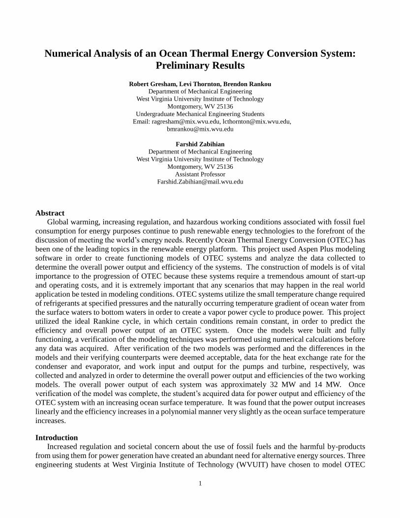
Technological limitations are the primary drawback to OTEC plants being widely used. Not only are
the systems very expensive, but calculated efficiencies of OTEC generally range from 6% to 7% with
actual systems only yielding around 3% to 4% [4]. This means that in order to produce a substantial
amount of power, the OTEC has to pump a lot of water. For an open system OTEC plant to produce 100
MW of power, 400 m3/s of 26˚C water would have to be pumped a distance of 20 m along the surface
through a 16 m diameter pipe and then recirculated to a depth of 1000 m to 4˚C water and back again [1].
With this large amount of water movement there is also the environmental effects to consider. Along with
these concerns, OTEC currently need certain ocean depths and temperature difference which are only
found in select areas around the equator as seen in Figure 1.
Figure 1. Distribution of global surface temperature [5]
Despite its drawbacks, OTEC systems still have promise. The energy that OTEC attempts to harvest
is created by a temperature gradient between the warmer surface water of the ocean and the colder water
on the bottom [1]. In order to produce any considerable energy a minimum temperature gradient of 20°C
is the current standard [1]. The average year around surface temperature in tropical regions is
approximately 28°C, and the temperature, at the standard used depth of 1000m, is relatively constant at
4°C [5]. In a sense this is a form of solar energy, but unlike other systems used to convert solar energy to
electricity, the temperature difference between the surface and the ocean bottom is more stable from night-
to-day and from season to season, meaning that OTEC systems can be run continuously where other forms
of solar energy converters have prolonged down time when conditions don’t provide ample sunlight [6].
It is estimated that approximately 107 MW of power could be provided from ocean thermal energy. This
abundance of renewable, continuous power is what makes OTEC research and development such a
promising field.
3
Theory
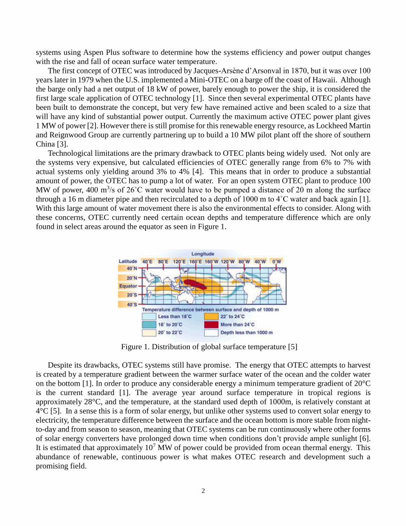
In order to better understand the closed OTEC system power cycle that was modeled, it is easier to
first consider the steam power plant cycle in its simplest conceptual form. In a steam power plant cycle
there are four main processes: the pump, boiler, turbine, and condenser [7]. First water is pumped to the
boiler in order to increase the pressure, then boiled and turned to steam [7]. The steam then enters the
turbine and expands to create mechanical work, and finally the steam at the outlet of the turbine is
condensed back to saturated liquid water so it can undergo the process again [7]. The steam power cycle
can be seen in Figure 2.
Figure 2. Steam power plant cycle
The steam power plant cycle is worth mentioning because the only difference in it and the OTEC cycle
models in this report is that instead of a boiler during the heating process, an evaporator is used, which in
most cases is a heat exchanger [1]. Although the concepts are very similar, there is a great difference in
the working fluids, which makes application and implementation of each process very different, but for
analysis purposes, the calculations and modeling techniques of ideal cycles are very similar. This is
explained in greater detail in the Methods section of this report.
When the concept was first introduced by d’Arsonval it was based on a closed system where the
working fluid, ammonia, is pumped from the low temperature at the bottom of the ocean to the high
temperature at the surface [2]. Because ammonia has a very low boiling point, the difference in
temperature of about 20 ˚C is enough to cause it to expand, at which point it is sent through a turbine
where the energy is converted from mechanical to electrical energy. As mentioned above, the working
fluid in a closed system will have to have properties that allow it to vaporize to a gaseous state at
approximately 28 ˚C and condense back to a liquid state around 4 ˚C in order to produce a large enough
pressure difference to create a worthwhile amount of mechanical work in the turbine. The most commonly
used working fluids in the closed OTEC systems are ammonia and propylene, and although other
refrigerants have been modeled, the majority of them are hazardous to the environment as well as any
worker that might be exposed to them [8]. The hazardous nature of refrigerants other than ammonia has
all but completely ruled them out as feasible working fluids [8].
More recently several experimental plants have been designed, and some tested, to use an open system
where the ocean water is the working fluid. This process is much more complicated, however there are
added benefits, because in the open system desalination is part of the process creating fresh water as a
byproduct that can be pumped to main lands for irrigation and even to processing plants for clean drinking
water [5].
The students decided on modeling a closed system due to the feasibility of modeling with their current
thermodynamic knowledge. As previously stated, the closeness of the closed OTEC system to the steam
power plant cycle makes for a very understandable thermodynamic cycle, of which the students had prior
knowledge and felt confident modeling. Other complications that arise with modeling an open OTEC
system are the desalination process and the even larger amount of ocean water that must be moved, the
4
movement of that which could have effects on the ocean wildlife in surrounding areas as well as the
temperature of the ocean [9].
Method
In order to obtain accurate data from OTEC models using the Aspen Plus modeling software, first the
modeling techniques had to be verified. In order to do so, two initial models were created. The first model
was a Rankine power cycle, which was verified by hand calculations. The second was a Carnot power
cycle, which mimicked the work of D. Bharathan’s Carnot Cycle OTEC [1] model using the same
software. Each model was verified based on percent error comparisons of the work and power
consumptions and extractions for each process in the cycle. These verification models are discussed in
further detail below.
Numerical Calculation Verification
As previously stated, the OTEC closed system power cycle is very similar to that of the steam power
plant cycle. With this in mind, the first verification test was performed by making hand calculations
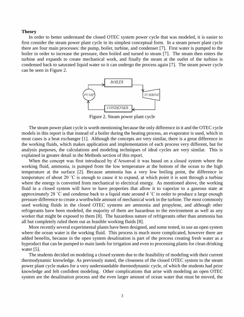
based on an ideal Rankine OTEC cycle with ammonia as the working fluid. In the ideal Rankine cycle
the processes occur as follows, along with the T-s diagram of the cycle, Figure 3 [7]:
1-2: Isentropic compression of working fluid to compressed liquid.
2-3: Heat transfer to the working fluid at a constant pressure as the fluid moves from compressed
liquid to saturated vapor.
3-4: Isentropic expansion of the working fluid to a liquid-vapor mixture.
4-1: Heat transfer from the fluid at a constant pressure as the fluid moves from a liquied-vapor
mixture to saturated liquid.
Figure 3. Temperature (T) vs. entropy (s) diagram of ideal Rankine OTEC power cycle
Roughly following the basic parameters set out in D. Bharathan’s OTEC model [2], it was assumed
that the pump inlet pressure was 6 bar, the turbine inlet pressure was 9 bar, and the mass flow rate of
ammonia through the system was 580 kg/s. Also in doing the numerical calculations all the ideal Rankine
cycle assumptions listed above were used.
The first step in this process is to identify the defining characteristics at each point (1, 2, 3, and 4) in
the cycle. Included below are these defining characteristics along with a brief description of how they
were found and/or calculated. Values from the ammonia saturated vapor-liquid and superheated steam
tables were taken from [7].
Point 1:
The pressure at 1 is specified in the assumptions, and T, h, v, and s are all values from the tables for
saturated liquid ammonia at a pressure of 6 bar.
5
P1 = 6 bar
T1 = 9.27 °C
h1 = 223.32 kJ/kg
v1 = 1.5982*10-3 m3/kg
Point 2:
P2 = 9 bar
h2 = 223.800 kJ/kg
The pressure at 2 is specified from the assumptions at 9 bar. In order to calculate h at 2, it was
considered that the specific work of the pump is characterized by the following equation for the specific
work of a control volume process (1).
𝑤 = ∫ 𝑣𝑑𝑝 = 𝑣(𝑝2 − 𝑝1)2
1 (1)
Maintaining the specific volume at point one and considering the given pressures at points 1 and 2, work
can be calculated as w = 0.4795 kJ/kg. Using this value in equation (2) where both work and h1 are known,
the enthalpy at point 2 is found.
𝑤 = ℎ2 − ℎ1 (2)
P2 = 9 bar
h2 = 223.800 kJ/kg
Point 3:
The pressure at 2 and 3 is equal because of the ideal Rankine cycle assumption of heat transfer to the
working fluid at constant pressure. The values for s3 and h3 are both found using the superheated vapor
tables and interpolation. Although the temperature at 3 is not necessary for the work and heat transfer
calculations, it is noted here because it had to vary slightly from the ideal Rankine cycle assumption. In
the ideal Rankine cycle, it is assumed that the state of the working fluid at 3 is saturated vapor, however,
because the Aspen Plus software value for saturated vapor was different from the value in [8], the students
chose to use a value of T3 = 22 °C instead of 21.52 °C, the value listed in the table. Even though this is a
slight deviation from the intended cycle, it is still a valid argument for the verification with a difference
in temperature of less than 0.5 °C.
P3 = 9 bar
s3 = 5.0722 kJ/kg-K
h3 = 1462.40 kJ/kg-K
T3 = 22 °C
Point 4:
The pressure at 1 and 4 is equal because of the ideal Rankine cycle assumption of heat transfer from
the working fluid at constant pressure. It is visible from Figure 3 that the process from 3 to 4 is at a
constant entropy, therefore s3 = s4. Considering the state of the working fluid is a liquid-vapor mixture at
4, the quality of the mixture can be calculated using equation (3), and using that quality along with values
from the tables and equation (4), the enthalpy at 4 is calculated.
𝑠 = 𝑠𝑓 + 𝜒(𝑠𝑔 − 𝑠𝑓) (3)
ℎ = ℎ𝑓 + 𝜒(ℎ𝑔 − ℎ𝑓) (4)
P4 = 6 bar
s4 = 5.0722 kJ/kg-K
χ4 = 0.9658
h4 = 1409.12 kJ/kg-K

6
Once each point was fully defined, the work input to the pump, the work output of the turbine, and the
heat transfer to and from the working fluid were calculated using the following equations.
Ẇ𝑝𝑢𝑚𝑝 = ṁ(ℎ2 − ℎ1) (5)
Ẇ𝑡𝑢𝑟𝑏𝑖𝑛𝑒 = ṁ(ℎ3 − ℎ4) (6)
˙𝑄𝑒𝑣𝑎𝑝𝑜𝑟𝑎𝑡𝑜𝑟 = ṁ(ℎ3 − ℎ2) (7)
˙𝑄𝑐𝑜𝑛𝑑𝑒𝑛𝑠𝑜𝑟 = ṁ(ℎ4 − ℎ1) (8)
Once the values for power and heat transfer rate were calculated from the numerical calculation, an
OTEC model was built in Aspen plus following the same cycle with the same assumptions made for
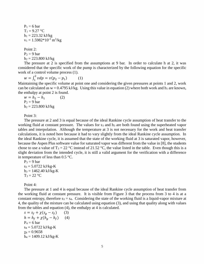
temperature, pressure, and ideal Rankine cycle and the results of each were compared. A detailed
schematic of the model can be found Figure 4. Table 1 shows this comparison using percent difference,
the equation for which is listed below.
% 𝐷𝑖𝑓𝑓𝑒𝑟𝑒𝑛𝑐𝑒 = |𝐴𝑐𝑡𝑢𝑎𝑙−𝐶𝑎𝑙𝑐𝑢𝑙𝑎𝑡𝑒𝑑|
𝐴𝑐𝑡𝑢𝑎𝑙× 100% (9)
Table 1. Verification of OTEC model with numerical calculations
From Table 1, it is clear that the percent difference from the model to the numerical calculations is
acceptable. The only percent difference that is larger than 5 % is that of the turbine. This is still acceptable
though, and it is important to consider that the method that the Aspen plus software uses to calculate the
power output could be a very complicated iterative solution that could not be duplicated by hand
calculations in a timely manner.
The only item not taken into consideration in this verification is the flow rate of warm and cold water
to the evaporator and condenser, respectively. Although these values are important when considering the
overall power output, since this verification focuses solely on the thermodynamic cycle of the working
fluid, these flow rates are not necessary to include in the verification process. The flow rates were chosen
by finding a value that ensured enough heat could be transferred to and from the working fluid in the
evaporator and condenser.
OTEC Model Verification
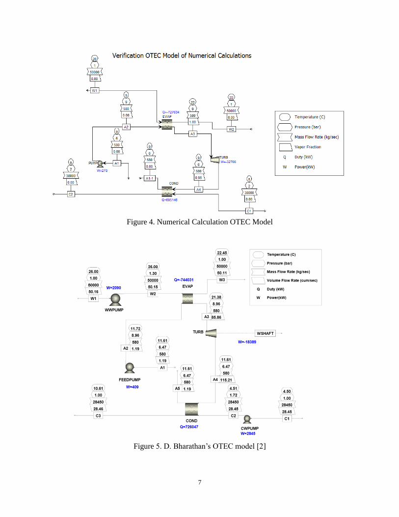
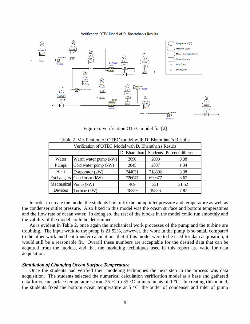
The second verification process that was performed used the OTEC model created in [2] and a
duplicate model that was created to ensure that the values were reasonably close. In order to do so, the
students used temperature and pressure values from [2] and the knowledge of the OTEC power cycle in
order to create a model that mimicked that of [2]. Once the model was created, a similar table to the
numerical calculation was created in order to ensure that the values were matched up properly. This table,
Table 2, is included below, along with Figure 5, the OTEC model created by [2]. The students Aspen Plus
model and detailed schematic is seen in Figure 6.
Numerical Aspen Model Percent difference
Evaporator (kW) 717558 727634 1.40
Condensor (kW) 687764 695146 1.07
Pump (kW) 278 278 0.00
Turbine (kW) 30902 32766 6.03
Verification of OTEC Model with Numerical Calculations
Heat
Exchangers
Mechanical
Devices
7
Figure 4. Numerical Calculation OTEC Model
Figure 5. D. Bharathan’s OTEC model [2]
8
Figure 6. Verification OTEC model for [2]
Table 2. Verification of OTEC model with D. Bharathan’s Results
In order to create the model the students had to fix the pump inlet pressure and temperature as well as
the condenser outlet pressure. Also fixed in this model was the ocean surface and bottom temperatures
and the flow rate of ocean water. In doing so, the rest of the blocks in the model could run smoothly and
the validity of the model could be determined.
As is evident in Table 2, once again the mechanical work processes of the pump and the turbine are
troubling. The input work to the pump is 21.52%, however, the work in the pump is so small compared
to the other work and heat transfer calculations that if this model were to be used for data acquisition, it
would still be a reasonable fit. Overall these numbers are acceptable for the desired data that can be
acquired from the models, and that the modeling techniques used in this report are valid for data
acquisition.
Simulation of Changing Ocean Surface Temperature
Once the students had verified their modeling techniques the next step in the process was data
acquisition. The students selected the numerical calculation verification model as a base and gathered
data for ocean surface temperatures from 25 °C to 35 °C in increments of 1 °C. In creating this model,
the students fixed the bottom ocean temperature at 5 °C, the outlet of condenser and inlet of pump
D. Bharathan Students Percent difference
Warm water pump (kW) 2090 2098 0.38
Cold water pump (kW) 2845 2807 1.34
Evaporator (kW) 744031 718892 3.38
Condensor (kW) 726047 699377 3.67
Pump (kW) 409 321 21.52
Turbine (kW) 18389 19836 7.87
Verification of OTEC Model with D. Bharathan's Results
Water
Pumps
Heat
Exchangers
Mechanical
Devices
9
temperature and pressure at 9.27 °C and 6 bar, respectively, and the difference in temperature of ammonia
and ocean water at the outlet of the evaporator at 1.2 °C. This value of temperature difference was cited
in [1] as a standard heat exchanger value. Also important to note here is that the isentropic and mechanical
efficiencies of the pump and turbine are set to 1, so the model portrays an ideal Rankine cycle with no
losses due to irreversibility during expansion or compression, and the outlet pressures of the pump and
turbine are fixed at 9 bar and 6 bar respectively in accordance with the ideal Rankine cycle.
RESULTS
Verification
Once the verification process was complete, the students were able to analyze their models based on
overall power output and efficiency of each of the models created. In order to calculate the efficiency of
each cycle, Equation (10) was used. The results are included in Table 3.
𝜂 =Ẇ𝑛𝑒𝑡
˙𝑄𝐻 (10)
Table 3. Energy Analysis Results of OTEC Models
These results are normal compared to the information given in the Introduction and Theory sections
of this report. However it is important to note a couple of things here.
The first noteworthy item is that the OTEC model used in the numerical calculations verification does
not include pumps that push the warm and cold ocean waters into the evaporator and condenser. Had
these values been included in this calculation, the efficiency of the numerical calculation model would
have been lower.
Simulation of Changing Ocean Surface Temperature
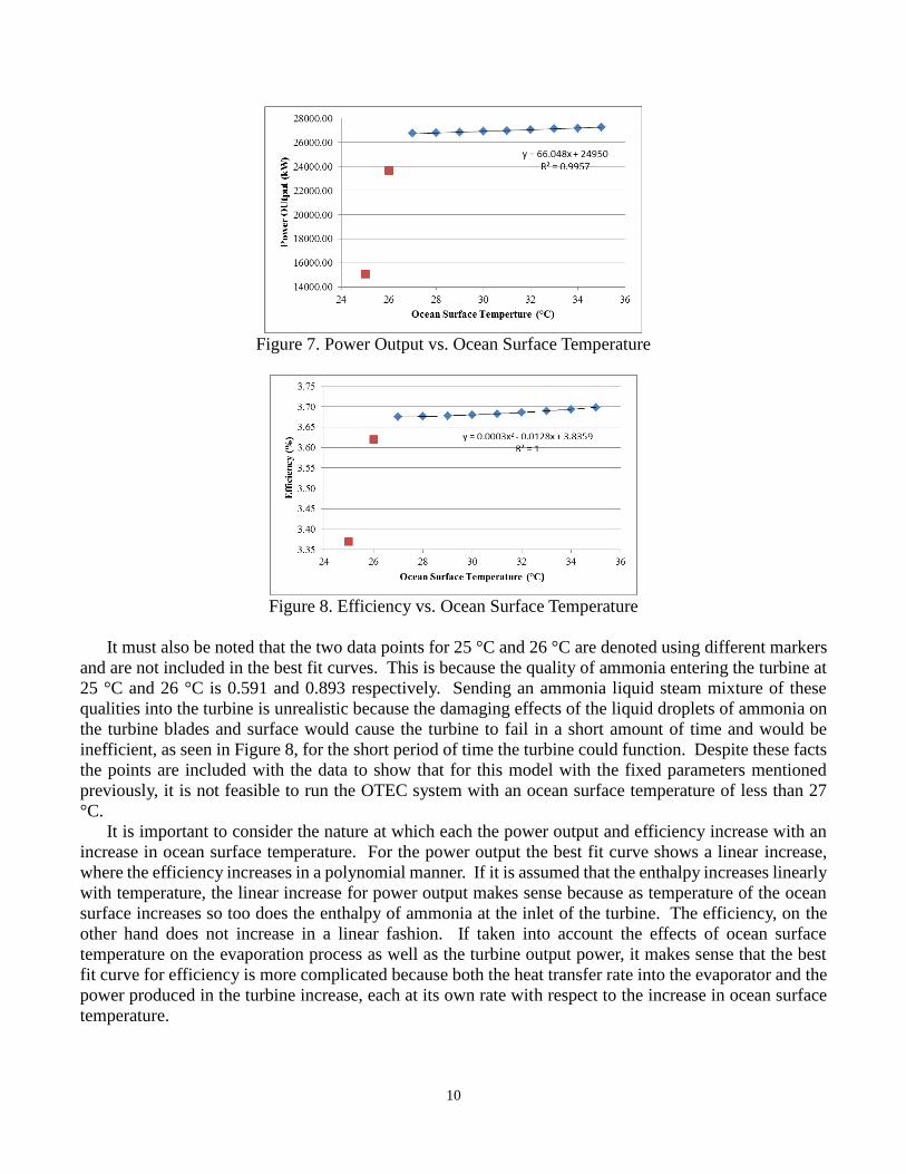
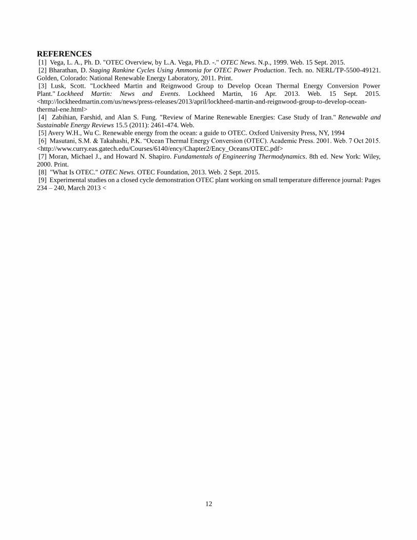
Using Equations 5 through 10 and simulation data from the previously mentioned OTEC model, the
students found that power output increases linearly and constantly as the ocean surface temperature
increases, and, although very slightly, efficiency of the cycle also increases. The results have been
included in Figures 7 and 8, charting power output and efficiency, respectively, as a dependent variable
and ocean surface temperature as the independent variable.
The simulation data shows that both power output and efficiency increase slightly as the ocean surface
temperature rises. Included in the plots is a best fit curve. These curves show that where power output
increases linearly with an increase in ocean surface temperature, the efficiency of the OTEC system
increases as a polynomial function with respect to the rising ocean surface temperature. Both best fit
curves show and R2 value of greater than 0.99 showing that they are good fits.
Wnet (kW) Efficiency (%)
Numerical Calculations Model 32488 4.53
OTEC Verification Model 14610 2.03
Energy Analysis of OTEC Models
10
Figure 7. Power Output vs. Ocean Surface Temperature
Figure 8. Efficiency vs. Ocean Surface Temperature
It must also be noted that the two data points for 25 °C and 26 °C are denoted using different markers
and are not included in the best fit curves. This is because the quality of ammonia entering the turbine at
25 °C and 26 °C is 0.591 and 0.893 respectively. Sending an ammonia liquid steam mixture of these
qualities into the turbine is unrealistic because the damaging effects of the liquid droplets of ammonia on
the turbine blades and surface would cause the turbine to fail in a short amount of time and would be
inefficient, as seen in Figure 8, for the short period of time the turbine could function. Despite these facts
the points are included with the data to show that for this model with the fixed parameters mentioned
previously, it is not feasible to run the OTEC system with an ocean surface temperature of less than 27
°C.
It is important to consider the nature at which each the power output and efficiency increase with an
increase in ocean surface temperature. For the power output the best fit curve shows a linear increase,
where the efficiency increases in a polynomial manner. If it is assumed that the enthalpy increases linearly
with temperature, the linear increase for power output makes sense because as temperature of the ocean
surface increases so too does the enthalpy of ammonia at the inlet of the turbine. The efficiency, on the
other hand does not increase in a linear fashion. If taken into account the effects of ocean surface
temperature on the evaporation process as well as the turbine output power, it makes sense that the best
fit curve for efficiency is more complicated because both the heat transfer rate into the evaporator and the
power produced in the turbine increase, each at its own rate with respect to the increase in ocean surface
temperature.

11
CONCLUSIONS
The students were able to create a working model of an OTEC system using the Aspen Plus software
and were able to use the model in order to collect data as to how the system would operate with changing
surface water temperatures. The conclusions they were able to draw from the data gathered were
pertaining to the nature of the increase in power output and efficiency of the system as well as the lower
limit of operating conditions for a system with the given pressures and flow rates.
Although the power output and efficiency of the OTEC system increase with rising ocean surface
temperatures, this increase is very slight and especially for efficiency. It seems to be a good assumption
that given these conditions that the OTEC system would be able to handle the power output increases
displayed in Figure 7 because they are so slight. Also the quality of the vapor gas mixture exiting the
turbine was never found to be less than 0.98, which is reasonable for the turbine to operate properly
without extensive mechanical damage occurring on the inside of the turbine due to the formation of liquid
ammonia droplets inside the turbine as expansion occurs.
However, most notable from these findings is the apparent lower limit of the ocean surface temperature
of 27 °C. This value could prove to be a large contributing factor to the sites at which the OTEC system
given similar parameters could be placed as well as the type of temperature drop that the system could
handle effectively. These drops in temperature could be due to severe weather or seasonal change, but
they must be taken into account so as not to damage or even destroy the turbine.
DISCUSSION
The importance of these types of modeling techniques and data acquisition is crucial in the current
OTEC design field. As stated in the introduction, OTEC systems can be very expensive and complicated,
and maintenance on these systems can be difficult, especially on elements of the system that are
completely submerged and fixed at great depths in the ocean. For this project the students chose to explore
how the changing surface temperature of the ocean can affect the efficiency and power output of the OTEC
system.
This shows only one aspect of the capabilities of modeling an OTEC system and how these models
can affect design and implementation of a system. Other considerations and data that could be collected
for future projects could include, but may not be limited to, change in bottom temperature, introduction
of isentropic and mechanical efficiencies to the expansion and compression processes, and varying heat
exchange rates and flow rates of ocean water and ammonia for better technologies. The possibilities for
this type of modeling are endless and could have a major effect on how an OTEC system is ultimately
designed and ultimately implemented.
Also important to note here is that the limited time frame the students had to work with the models
and the Aspen Plus software made it hard to implement everything they would have liked to in order to
present a more accurate model of a fully functioning system. The software has the capability of
introducing pump and turbine efficiency curves for more a more accurate assessment of the mechanical
work required or produced in these systems, as well as several heat transfer models that could be explored
and used in order to more accurately assess the evaporator and condenser components. The modeling
possibilities are endless. Although the students did not have the time to explore all these options, the fact
that they were able, with the help of their advisor, to learn the basic functions of Aspen Plus and create a
working model, all outside of the scheduled class time, shows the type of achievement undergraduate
students can have when they are motivated and have a motivated faculty behind them. It is the hope of
the students that these types of projects are continued at WVU TECH and institutions all over the country,
because these types of independent learning activities that show the full potential of undergraduate
engineering students.
12
REFERENCES [1] Vega, L. A., Ph. D. "OTEC Overview, by L.A. Vega, Ph.D. -." OTEC News. N.p., 1999. Web. 15 Sept. 2015.
[2] Bharathan, D. Staging Rankine Cycles Using Ammonia for OTEC Power Production. Tech. no. NERL/TP-5500-49121.
Golden, Colorado: National Renewable Energy Laboratory, 2011. Print.
[3] Lusk, Scott. "Lockheed Martin and Reignwood Group to Develop Ocean Thermal Energy Conversion Power
Plant." Lockheed Martin: News and Events. Lockheed Martin, 16 Apr. 2013. Web. 15 Sept. 2015.
<http://lockheedmartin.com/us/news/press-releases/2013/april/lockheed-martin-and-reignwood-group-to-develop-ocean-
thermal-ene.html>
[4] Zabihian, Farshid, and Alan S. Fung. "Review of Marine Renewable Energies: Case Study of Iran." Renewable and
Sustainable Energy Reviews 15.5 (2011): 2461-474. Web.
[5] Avery W.H., Wu C. Renewable energy from the ocean: a guide to OTEC. Oxford University Press, NY, 1994
[6] Masutani, S.M. & Takahashi, P.K. “Ocean Thermal Energy Conversion (OTEC). Academic Press. 2001. Web. 7 Oct 2015.
<http://www.curry.eas.gatech.edu/Courses/6140/ency/Chapter2/Ency_Oceans/OTEC.pdf>
[7] Moran, Michael J., and Howard N. Shapiro. Fundamentals of Engineering Thermodynamics. 8th ed. New York: Wiley,
2000. Print.
[8] "What Is OTEC." OTEC News. OTEC Foundation, 2013. Web. 2 Sept. 2015.
[9] Experimental studies on a closed cycle demonstration OTEC plant working on small temperature difference journal: Pages
234 – 240, March 2013 <