Embed Size (px)
Citation preview

Master of Science Thesis
KTH School of Industrial Engineering and Management
Department of Energy Technology
Division of Heat and Power Technology
100 44 Stockholm, Sweden
Numerical analysis of aerodynamic
damping in a transonic compressor
Vincenzo Stasolla
Master thesis 2019

-2-
-3-
Master of Science Thesis EGI 2019: TRITA-
ITM-EX 2019:612
Numerical analysis of aerodynamic damping
in a transonic compressor
Vincenzo Stasolla
Approved
Date 2019-09-11
Examiner
Björn Laumert
Supervisor
Nenad Glodic
Commissioner
Contact person
ABSTRACT
Aeromechanics is one of the main limitations for more efficient, lighter, cheaper and reliable turbomachines,
such as steam or gas turbines, as well as compressors and fans. In fact, aircraft engines designed in the last
few years feature more slender, thinner and more highly loaded blades, but this trend gives rise to increased
sensitivity for vibrations induced by the fluid and result in increasing challenges regarding structural integrity
of the engine. Forced vibration as well as flutter failures need to be carefully avoided and an important
parameter predicting instabilities in both cases is the aerodynamic damping.
The aim of the present project is to numerically investigate aerodynamic damping in the first rotor of a
transonic compressor (VINK6). The transonic flow field leads to a bow shock at each blade leading edge,
which propagates to the suction side of the adjacent blade. This, along with the fact that the rotating blade
row vibrates in different mode shapes and this induces unsteady pressure fluctuations, suggests to evaluate
unsteady flow field solutions for different cases. In particular, the work focuses on the unsteady aerodynamic
damping prediction for the first six mode shapes. The aerodynamic coupling between the blades of this
rotor is estimated by employing a transient blade row model set in blade flutter case. The commercial CFD
code used for these investigations is ANSYS CFX.
Aerodynamic damping is evaluated on the basis of the Energy Method, which allows to calculate the
logarithmic decrement employed as a stability parameter in this study. The least logarithmic decrement
values for each mode shape are better investigated by finding the unsteady pressure distribution at different
span locations, indication of the generalized force of the blade surface and the local work distribution, useful
to get insights into the coupling between displacements and consequent generated unsteady pressure. Two
different transient methods (Time Integration and Harmonic Balance) are employed showing the same trend
of the quantities under consideration with similar computational effort. The first mode is the only one with
a flutter risk, while the higher modes feature higher reduced frequencies, out from the critical range found
in literature. Unsteady pressure for all the modes is quite comparable at higher span locations, where the
largest displacements are prescribed, while at mid-span less comparable values are found due to different
amplitude and direction of the mode shape. SST turbulence model is analyzed, which does not influence in
significant manner the predictions in this case, with respect to the k-epsilon model employed for the whole

-4-
work. Unsteady pressure predictions based on the Fourier transformation are validated with MATLAB
codes making use of Fast Fourier Transform in order to ensure the goodness of CFX computations.
Convergence level and discrepancy in aerodamping values are stated for each result and this allows to
estimate the computational effort for every simulation and the permanent presence of numerical
propagation errors.
Keywords: transonic compressor, flutter, vibration, CFD
-5-
SAMMANFATTNING
Aeromekanik är en av huvudbegränsningarna för mer effektiva, lättare, billigare och mer pålitliga
turbomaskiner, som ångturbiner, gasturbiner, samt kompressorer och fläktar. I själva verket har
flygplansmotorer som designats under de senaste åren har fått tunnare och mer belastade skovlar, men
denna trend ger upphov till ökad känslighet för aeromekaniska vibrationer och resulterar i ökande
utmaningar när det gäller motorns strukturella integritet. Aerodynamiskt påtvingade vibrationer såväl som
fladder måste predikteras noggrant för att kunna undvikas och en viktig parameter som förutsäger instabilitet
i båda fallen är den aerodynamiska dämpningen.
Syftet med det aktuella projektet är att numeriskt undersöka aerodynamisk dämpning i den första rotorn
hos en transonisk kompressor (VINK6). Det transoniska flödesfältet leder till en bågformad stötvåg vid
bladets främre kant, som sprider sig till sugsidan på det intilliggande bladet. I och med detta, tillsammans
med det faktum att den roterande bladraden vibrerar i olika modformer och detta inducerar instationära
tryckfluktuationer, syftar detta arbete på att utvärdera flödesfältslösningar för olika fal. I synnerhet fokuserar
arbetet på prediktering av den instationära aerodynamiska dämpningen för de första sex modformen. Den
aerodynamiska kopplingen mellan bladen hos denna rotor uppskattas genom att använda en transient
bladradmodell uppsatt för fladderberäkningen. Den kommersiella CFD-koden som används för denna
utredning är ANSYS CFX.
Aerodynamisk dämpning utvärderas med hjälp av energimetoden, som gör det möjligt att beräkna den
logaritmiska minskningen som används som en stabilitetsparameter i denna studie. De minsta logaritmiska
dekrementvärdena för varje modform undersöks bättre genom att hitta den ostadiga tryckfördelningen på
olika spannpositioner, som är en indikering av den lokala arbetsfördelningen, användbar för att få insikt i
kopplingen mellan förskjutningar och därmed genererat ostabilt tryck. Två olika transienta metoder används
som visar samma trend för de kvantiteter som beaktas med liknande beräkningsinsatser. Den första
modformen är den enda med en fladderrisk, medan de högre modformerna har högre reducerade
frekvenser, och ligger utanför det kritiska intervallet som finns i litteraturen. Instationärt tryck för alla moder
är ganska jämförbart på de högre spannpositioner, där de största förskjutningarna föreskrivs, medan runt
midspannet finns mindre jämförbara värden på grund av olika amplitud och riktning för modformen. SST-
turbulensmodellen analyseras, som i detta fall inte påverkar predikteringen på ett betydande sätt. Det
predikterade instationära trycket baserad på Fourier-transformationen valideras med MATLAB-koder som
använder sig av Fast Fourier Transform för att säkerställa noggrannheten hos CFX-beräkningar.
Konvergensnivå och skillnader i aerodämpningsvärden anges för varje resultat och detta gör det möjligt att
uppskatta beräkningsinsatsen för varje simulering och uppskatta utbredningen av det numeriska felet.
Nyckelord: transonic kompressor, fladder, vibration, CFD

-6-
ACKNOWLEDGMENTS
The present work has been developed at Royal Institute of Technology in collaboration with Politecnico di
Torino, the support of which is gratefully acknowledged. Thanks to these two institutions, I improved
myself in different contexts and I had the opportunity to broaden my horizons.
I would like to express my gratitude to Prof. Björn Laumert at the Chair of Heat and Power Technology at
KTH, for giving me opportunity to perform this work at the department.
I am extremely thankful to my supervisor Nenad Glodic at KTH for his offer of the thesis and for his
guidance and enthusiastic support in solving the problems faced along this path. Thanks for having involved
me in the THRUST Master Program at KTH, where I met new professors and students from whom I could
work with and learn new skills.
Thanks to Prof. Antonio Mittica for having accepted to be my supervisor at Politecnico di Torino and for
his confidence on my work.
Special thanks to Mauricio Gutierrez Salas, my co-supervisor and postdoctoral researcher at KTH, for his
constant insightful tips and important feedbacks, which allowed me to further investigate the suspected
aspects and find an optimal solution.
Fundamental has been the support of my mate Salvatore Guccione, with whom I took some courses at
KTH and studied together. His advices helped me keep always motivated and overcome every kind of
difficulty.
Thanks to all the new friends I met in this wonderful year in Sweden, especially to Alex, Pietro, Marta,
Simone, Edoardo, Mara, Giulia, Antonella and all the other people from Björksätra. Thanks to my friends
in Italy for always being present.
Endless gratitude goes to my family and in particular to my parents, who have always supported me in every
day of my study carrier and have been a warm light especially during hard times. Without them all this would
not have been possible!
-7-
Table of Contents
ABSTRACT ................................................................................................................................................................... 3
SAMMANFATTNING ........................................................................................................................................ 5
ACKNOWLEDGMENTS ......................................................................................................................................... 6
NOMENCLATURE..............................................................................................................................................13
1 BACKGROUND ..............................................................................................................................................18
1.1 The emergence of aeroelasticity ..............................................................................................................18
1.2 Fluid-structural equation and forced response for a SDOF system .................................................19
1.3 Modal analysis and forced response for a MDOF system .................................................................22
1.4 Flutter phenomenon .................................................................................................................................24
1.5 Transonic flow in axial compressor .......................................................................................................25
1.6 Introduction to numerical modeling and CFD-FEM methods .........................................................27
2 THEORETICAL APPROACH ......................................................................................................................29
2.1 Unsteady surface pressure and aerodynamic coupling ........................................................................29
2.2 Aerodynamics and mode shapes interaction ........................................................................................30
2.3 Theoretical methods for aerodamping predictions .............................................................................31
2.3.1 Travelling wave mode analysis and energy method ...................................................................32
2.3.2 Aerodynamic Influence Coefficient method (or direct approach)...........................................36
3 OBJECTIVE ......................................................................................................................................................40
4 TEST CASE DESCRIPTION AND PREVIOUS WORKS ....................................................................41
4.1 Transonic compressor specifications .....................................................................................................41
4.2 Aeromechanical assessment ....................................................................................................................42
4.3 Previous work on VINK6 blading .........................................................................................................44
5 NUMERICAL METHODS.............................................................................................................................46
5.1 Computational environment ...................................................................................................................46
5.2 Use of RANS equations and turbulence models .................................................................................46
5.3 Fourier transformation method ..............................................................................................................49
5.4 Harmonic balance analysis .......................................................................................................................50
6 METHODOLOGY AND DESCRIPTION OF THE MODELS ..........................................................53
6.1 Spatial discretization .................................................................................................................................53
6.2 Steady-state modeling ...............................................................................................................................54
6.3 Transient blade row modeling ................................................................................................................57
6.4 FEM structural analysis ............................................................................................................................58
6.5 Unsteady numerical modeling (time integration method) ..................................................................58
6.6 Harmonic Balance method ......................................................................................................................60
7 RESULTS AND DISCUSSION .....................................................................................................................62
-8-
7.1 Steady-state results for first stage computation ....................................................................................62
7.2 Steady-state results for first rotor computation ...................................................................................67
7.3 Unsteady results .........................................................................................................................................69
7.4 S-shape overview for Time Integration method ..................................................................................70
7.5 Convergence and discrepancy for higher mode predictions ..............................................................75
7.6 Unsteady results for each mode ..............................................................................................................76
7.6.1 First mode with k-epsilon model...................................................................................................77
7.6.2 Second mode with k-epsilon model ..............................................................................................79
7.6.3 Third mode with k-epsilon model .................................................................................................81
7.6.4 Fourth mode with k-epsilon model ..............................................................................................83
7.6.5 Fifth mode with k-epsilon model ..................................................................................................85
7.6.6 Sixth mode with k-epsilon model ..................................................................................................87
7.6.7 Unsteady pressure overview for all the modes............................................................................88
7.7 First mode investigation ...........................................................................................................................90
7.7.1 ND investigation ..............................................................................................................................91
7.7.2 Turbulence model investigation ....................................................................................................93
7.8 Fourth mode investigation ......................................................................................................................94
7.8.1 CFX convergence study ..................................................................................................................94
7.8.2 Scaling factor analysis ......................................................................................................................96
7.9 Fourier transformation investigation .....................................................................................................96
7.9.1 Fourier transformation for first mode ..........................................................................................97
7.9.2 Fourier transformation for second mode ....................................................................................98
7.9.3 Fourier transformation for third mode ........................................................................................99
7.9.4 Fourier transformation for fourth mode................................................................................... 100
7.9.5 Other Fourier transformation trials for first mode ................................................................. 103
7.10 Harmonic balance comparisons .......................................................................................................... 104
7.10.1 S-shape comparisons .................................................................................................................... 104
7.10.2 Unsteady pressure coefficient comparisons ............................................................................. 107
8 CONCLUSION AND FUTURE WORK ................................................................................................. 109
Bibliography .............................................................................................................................................................. 111
-9-
List of Figures
Figure 1.1: Kegworth air disaster ..............................................................................................................................19
Figure 1.2: Triangle of forces created by Prof. A.R. Colar in 1947 [2] ...............................................................19
Figure 1.3: Aircraft engine structure and turbomachinery blade row [3] ...........................................................20
Figure 1.4: Module and phase of the structural displacement for forced response analysis [4] .....................21
Figure 1.5: Blade modes obtained from FEM analysis .........................................................................................22
Figure 1.6: Main disk modes ......................................................................................................................................23
Figure 1.7: Campbell diagram showing frequency ranges for common aeroelastic problems [5] ..................23
Figure 1.8: Rolls-Royce aeroengine ..........................................................................................................................24
Figure 1.9: Compressor map with flutter boundaries ............................................................................................25
Figure 1.10: Rotating transonic compressor blade row [8] ...................................................................................25
Figure 1.11: Bow shock at leading edge of a compressor rotor [8] .....................................................................26
Figure 1.12: Transonic axial compressor features [8] ............................................................................................27
Figure 2.1: Harmonic pressure due to harmonic motion......................................................................................29
Figure 2.2: Coupled blade and disk modes..............................................................................................................30
Figure 2.3: Stability plots, also called tie-dye plots [14] .........................................................................................31
Figure 2.4: Graphical representation of mass ratio ................................................................................................31
Figure 2.5: TWM for different nodal diameter patterns [12] ...............................................................................32
Figure 2.6: Combined blade mode shapes ...............................................................................................................33
Figure 2.7: Grafical representation of the logarithmic decrement .......................................................................36
Figure 2.8: Log-dec versus ND plot for AETR blade row [18] ...........................................................................36
Figure 2.9: Influence between adjacent blades .......................................................................................................37
Figure 2.10: Influence of blade 0, ± 1, ±2 (from the left to the right) .............................................................38
Figure 2.11: Characteristic stability curve ................................................................................................................38
Figure 2.12: Polar graph and circle plot of the imaginary versus real component ............................................39
Figure 4.1: Compressor layout shown in the meridional view [21] .....................................................................41
Figure 4.2: Campbell diagram for the first stage rotor blades (R1) [21] .............................................................43
Figure 4.3: Aerodynamic damping curve for mode 1 (on the left side) and mode 2 (on the right side) .......44
Figure 4.4: S-curve for the first three modes at design throttle and 70% speed ...............................................45
Figure 5.1: Double passage model ............................................................................................................................49
Figure 6.1: Comparison of different mesh refinements for the first compressor stage ...................................54
Figure 6.2: Total pressure, static pressure and velocity component trend at the machine inlet used as
boundary conditions ...................................................................................................................................................55
Figure 6.3: Model of plenum, rotor and stator for steady-state calculations .....................................................56
Figure 6.4: Application phase-shifted boundary conditions to a blade flutter case [23] ..................................57
Figure 6.5: TWM convention in ANSYS CFX [23] ...............................................................................................59
Figure 7.1: Blade loading comparison between k-epsilon and SST turbulence model for the coarse mesh 63
Figure 7.2: Blade loading comparison between k-epsilon and SST turbulence model for the medium mesh
........................................................................................................................................................................................64
Figure 7.3: Blade loading comparison between k-epsilon and SST turbulence model for the fine mesh .....64
Figure 7.4: Blade loading comparison with the three different mesh refinements in the model with k-epsilon
turbulence model .........................................................................................................................................................65
Figure 7.5: Blade loading comparison with the three different mesh refinements in the model with SST
turbulence model .........................................................................................................................................................65
Figure 7.6: Blade loading comparison at different span locations for the chosen steady setups ...................66
Figure 7.7: Comparison Mach number flow field for the medium mesh between k-epsilon (on the left) and
SST (on the right) turbulence model at 95% span .................................................................................................67
Figure 7.8: Comparison Mach number flow field for the fine mesh between k-epsilon (on the left) and SST
(on the right) turbulence model at 95% span .........................................................................................................67
-10-
Figure 7.9: Comparison between stage 1 and rotor 1 blade loading at 5% span ..............................................68
Figure 7.10: Comparison between stage 1 and rotor 1 blade loading at 50% span ..........................................68
Figure 7.11: Comparison between stage 1 and rotor 1 blade loading at 95% span ..........................................69
Figure 7.12: Logarithmic decrement distribution for the first mode using k-epsilon turbulence model and
deviation in predicted values between the two blades ...........................................................................................71
Figure 7.13: Logarithmic decrement distribution for the first mode using SST turbulence model and
deviation in predicted values between the two blades ...........................................................................................72
Figure 7.14: Logarithmic decrement distribution for the first mode comparing k-epsilon and SST turbulence
model and deviation in predicted values between the two models .....................................................................72
Figure 7.15: Logarithmic decrement distribution for the fourth mode using k-epsilon turbulence model and
deviation in predicted values between the two blades ...........................................................................................73
Figure 7.16: Logarithmic decrement distribution for the fifth mode using k-epsilon turbulence model and
deviation in predicted values between the two blades ...........................................................................................74
Figure 7.17: Logarithmic decrement distribution for the sixth mode using k-epsilon turbulence model and
deviation in predicted values between the two blades ...........................................................................................74
Figure 7.18: S-shape curve overview of all investigated modes for k-epsilon turbulence model ...................75
Figure 7.19: Unsteady pressure coefficient (amplitude and phase) and local work coefficient distribution for
the first mode with k-epsilon model at 50%, 90% and 95% span ......................................................................77
Figure 7.20: Blade displacements for the first mode .............................................................................................77
Figure 7.21: Unsteady pressure flow field for the first mode at 50% span (on the left) and 95% span (on the
right) ..............................................................................................................................................................................78
Figure 7.22: Unsteady pressure coefficient (amplitude and phase) and local work coefficient distribution for
the second mode with k-epsilon model at 50%, 90% and 95% span .................................................................79
Figure 7.23: Blade displacements for the second mode ........................................................................................79
Figure 7.24: Unsteady pressure flow field for the second mode at 50% span (on the left) and 95% span (on
the right) ........................................................................................................................................................................80
Figure 7.25: Unsteady pressure coefficient (amplitude and phase) and local work coefficient distribution for
the third mode with k-epsilon model at 50%, 90% and 95% span .....................................................................81
Figure 7.26: Blade displacements for the third mode ...........................................................................................81
Figure 7.27: Unsteady pressure flow field for the third mode at 50% span (on the left) and 95% span (on
the right) ........................................................................................................................................................................82
Figure 7.28: Unsteady pressure coefficient (amplitude and phase) and local work coefficient distribution for
the fourth mode with k-epsilon model at 50%, 90% and 95% span ..................................................................83
Figure 7.29: Blade displacements for the fourth mode .........................................................................................83
Figure 7.30: Unsteady pressure flow field for the fourth mode at 50% span (on the left) and 95% span (on
the right) ........................................................................................................................................................................84
Figure 7.31: Unsteady pressure coefficient (amplitude and phase) and local work coefficient distribution for
the fifth mode with k-epsilon model at 50%, 90% and 95% span ......................................................................85
Figure 7.32: Blade displacements for the fifth mode ............................................................................................85
Figure 7.33: Unsteady pressure flow field for the fifth mode at 50% span (on the left) and 95% span (on the
right) ..............................................................................................................................................................................86
Figure 7.34: Unsteady pressure coefficient (amplitude and phase) and local work coefficient distribution for
the sixth mode with k-epsilon model at 50%, 90% and 95% span .....................................................................87
Figure 7.35: Blade displacements for the sixth mode ............................................................................................87
Figure 7.36: Unsteady pressure flow field for the sixth mode at 50% span (on the left) and 95% span (on
the right) ........................................................................................................................................................................88
Figure 7.37: Unsteady surface pressure amplitude overview for all modes at 50% span ................................89
Figure 7.38: Unsteady surface pressure coefficient amplitude overview for all modes at 50% span ............89
Figure 7.39: Unsteady surface pressure amplitude overview for all modes at 95% span ................................90
Figure 7.40 : Unsteady surface pressure coefficient amplitude overview for all modes at 95% span ...........90
-11-
Figure 7.41: Comparison for the first mode at 95% span for different nodal diameters ................................91
Figure 7.42: Unsteady comparison for the first mode at 95% span between 𝑁𝐷 = 2 and 𝑁𝐷 = 3............92
Figure 7.43: Unsteady comparison for the first mode at 95% span between 𝑁𝐷 = 2 and 𝑁𝐷 = −15......92
Figure 7.44: Unsteady pressure coefficient distribution for the first mode comparing k-epsilon and SST
turbulence model .........................................................................................................................................................93
Figure 7.45 : Local work coefficient distribution for the first mode comparing k-epsilon and SST turbulence
model .............................................................................................................................................................................94
Figure 7.46: Unsteady pressure predictions for several periods in the fourth mode case ...............................95
Figure 7.47: Peak-to-Peak and Steady-Value torque error for fourth mode simulations ................................95
Figure 7.48: Unsteady pressure predictions for several scaling factors in the fourth mode case ...................96
Figure 7.49: Fourier transformation comparisons for the first mode at P=6 ...................................................97
Figure 7.50: Fourier transformation comparisons for the first mode at P=9 ...................................................98
Figure 7.51: Fourier transformation comparisons for the second mode at P=9 ..............................................99
Figure 7.52: Fourier transformation comparisons for the second mode at P=14 ............................................99
Figure 7.53: Fourier transformation comparisons for the third mode at P=9 ............................................... 100
Figure 7.54: Fourier transformation comparisons for the third mode at P=14 ............................................. 100
Figure 7.55: Fourier transformation comparisons for the fourth mode at P=6 ............................................ 101
Figure 7.56: Fourier transformation comparisons for the fourth mode at P=9 ............................................ 101
Figure 7.57: Fourier transformation comparisons for the fourth mode at P=15 .......................................... 102
Figure 7.58: Fourier transformation comparisons for the fourth mode at P=18 .......................................... 102
Figure 7.59: Fourier transformation comparisons for the fourth mode at P=23 .......................................... 103
Figure 7.60: Other Fourier transformation comparisons for the first mode at P=6..................................... 103
Figure 7.61 : Logarithmic decrement distribution for the first mode comparing time integration and
harmonic balance transient methods ..................................................................................................................... 105
Figure 7.62: Logarithmic decrement distribution for the fourth mode comparing time integration and
harmonic balance transient methods ..................................................................................................................... 105
Figure 7.63: Logarithmic decrement distribution for the fifth mode comparing time integration and
harmonic balance transient methods ..................................................................................................................... 106
Figure 7.64: Logarithmic decrement distribution for the sixth mode comparing time integration and
harmonic balance transient methods ..................................................................................................................... 106
Figure 7.65: Unsteady pressure coefficient comparison between Time Integration and Harmonic Balance
method for the first mode in the least stable condition ..................................................................................... 107
Figure 7.66: Unsteady pressure coefficient comparison between Time Integration and Harmonic Balance
method for the fourth mode in the least stable condition ................................................................................. 107
Figure 7.67: Unsteady pressure coefficient comparison between Time Integration and Harmonic Balance
method for the fifth mode in the least stable condition .................................................................................... 108
Figure 7.68: Unsteady pressure coefficient comparison between Time Integration and Harmonic Balance
method for the fifth mode in the least stable condition .................................................................................... 108

-12-
List of tables
Table 4.1: High-speed booster performance data ..................................................................................................41
Table 4.2: VINK compressor blade count ..............................................................................................................42
Table 4.3: Thermodynamic parameters of the first compressor stage at the design point..............................42
Table 4.4: Blade geometry of the first compressor stage ......................................................................................42
Table 5.1: Turbulence models ...................................................................................................................................48
Table 6.1: Mesh specifications (node count) for the first compressor stage .....................................................54
Table 6.2: Numerical setup of Stage 1 and Rotor 1 for steady-state simulation ...............................................56
Table 6.3: Reduced frequency for the first six mode shapes of rotor 1 VINK compressor ...........................59
Table 6.4: Time steps for different NDs [22] .........................................................................................................60
-13-
NOMENCLATURE
Latin Symbols
𝐴 blade oscillation amplitude
𝑐 blade chord, damping coefficient
𝑏 blade height
𝑐�̅� normalized steady pressure coefficient
�̂�𝑝 normalized unsteady pressure coefficient �̂�𝑝 =𝑝
𝐴∙𝑝𝑑𝑦𝑛
𝑑𝑓 infinitesimal force coefficient
𝑑𝑆 infinitesimal arcwise surface component, per unit of span
𝑑𝑍 displacement in axial direction
𝑓 oscillation frequency
𝑓 normalized unsteady force vector on span section
𝐹 harmonic force
�⃗� normalized unsteady force vector on blade
𝑝 pressure
�̅� mean pressure
�̃� time-varying pressure perturbation
�̂� complex pressure amplitude
ℎ⃗⃗ complex mode shape vector
ℎ structural motion
𝑖 imaginary unit, 𝑖 = √−1
𝑘 reduced frequency, based on full chord 𝑘 =2𝜋𝑓𝑐
𝑢
𝑙 nodal diameter
𝑚 mass
𝑀 Mach number, mass matrix, harmonic number (HB method)
-14-
𝐾 stiffness matrix, kinetic energy
k stiffness
C damping matrix
Q modal displacement vector
�⃗⃗� normal vector to surface element
𝑡 time, time of flight
∆𝑡 timestep size
𝑇 oscillation period
𝑢, 𝑣, 𝑤 Cartesian velocity components
𝑊𝑐𝑦𝑐𝑙𝑒 work per cycle
𝑥, 𝑦, 𝑧 Cartesian coordinates
x displacement
∆𝑥 mesh element size
�̇� first derivative of displacement
�̈� second derivative of displacement
r frequency ratio
𝑛,𝑚 blade indices
𝑒 unit vector
𝑅𝑒 real part
𝐼𝑚 imaginary part
𝑁 rotational speed, number
𝑆 stress matrix
Greek Symbols
𝛼 rotation angle, normalized blade oscillation amplitude 𝛼 =ℎ𝑚𝑎𝑥
𝑐
𝜖 turbulence dissipation rate
𝜁 damping ratio

-15-
𝜇 mass ratio
𝜋 pressure ratio
𝜌 density
𝜎 inter-blade phase angle
𝜔 rotational frequency, 𝜔 = 2𝜋𝑓
𝜃 phase lag between torsion and bending
Θ stability parameter
𝜙𝑝→ℎ phase angle of response with respect to excitation (motion); the phase
angle is per definition positive if the response is leading the excitation
𝜆 eigenvalue
Ω rotor speed
𝜔∗ critical reduced frequency
𝛿 logarithmic decrement
Subscripts
𝑖 inertial
𝑒 elastic
𝑎, 𝑎𝑒𝑟𝑜 aerodynmic
𝑑𝑎𝑚𝑝 damping
𝑑𝑖𝑠𝑡 disturbance
𝑛 natural
𝑟𝑒𝑓 reference
𝑑𝑦𝑛 dynamic
𝐵𝐿 blades
𝐿 lift
𝐹 force
𝑀 moment
−∞ machine inlet
-16-
𝐵 reference surface
𝑤 work
𝑎𝑣𝑒 average
Abbreviation
KTH Kungliga Tekniska Hogskolan
IBPA Inter-Blade Phase Angle
ND Nodal diameter
SDOF Single Degree Of Freedom
MDOF Multiple Degree of Freedom
TWM Travelling Wave Mode
VIGV Variable Inlet Guide Vanes
R Rotor
S Stator
ICC Inter-Cooling Channel
LPC Low Pressure compressor
HPC High Pressure Compressor
LPT Low Pressure Turbine
HPT High Pressure Turbine
CFD Computational Fluid Dynamic
SST Menter’s Shear Stress Transport
CPU Central Processing Unit
FEM Finite Element Model
VINK Virtual Integrated Compressor
ARIAS Advanced Research Into Aeromechanical Solution
RANS Reynolds Averaged Navier-Stokes
HCF High Cycle Fatigue
EO Engine Order

-17-
AIC Aerodynamic Influence Coefficient
1F, 1B First Bending
1T First Torsion
2B Second Bending
2T Second Torsion
3B Third Bending
1E First Edgewise Bending
FT Fourier transformation
FFT Fast Fourier Transformation
TS Time Steps
P Period
HB Harmonic Balance
HA Harmonic Analysis
TI Time Integration
SV Steady-Value
P2P Peak-to-Peak
-18-
1 BACKGROUND
Aeromechanics is one of the main limitations for more efficient, lighter, cheaper and reliable turbomachines,
such as steam or gas turbines, as well as compressors and fans. In fact, aircraft engines designed in the last
few years feature more slender, thinner and more highly loaded blades, but this tendency gives rise to
increased sensitivity for vibrations induced by the fluid and result in increasing challenges regarding
structural integrity of the engine.
The dominant mechanism causing failures in turbomachinery components is the high cycle fatigue (HCF),
which may arise from forced vibration as well as flutter, characterized by self-induced and self-sustained
oscillations leading to detrimental effects on the structure. The source of such phenomena is attributed to
a large spectrum of non-uniformity in the flow field around the regarded components, which creates
unsteadiness in time due to blade row interactions, structural motion or separation phenomenon. Therefore,
the structure will be stressed by aerodynamic forces depending on the unsteady surface pressure and it will
oscillate in different mode shapes.
Moreover, turbomachinery operations in a transonic flow field add influence of shocks, boundary layer
interactions and other unsteady flow effects. These phenomena interacting with the structure increase the
flow field complexity and might be another possible cause of vibration triggering and subsequent failures.
1.1 The emergence of aeroelasticity
Aeroelasticity is the term used to describe the study of the interaction between the deformation of an elastic
structural component exposed to a fluid flow and the resultant of the aerodynamic forces arising from the
flow field.
In the past, although the fluid-structural interaction had always been investigated, it was taken more in detail
into account with the advent of the Second World War, during which the requirement of high-performance
aircrafts became vital. Before then, in fact, aircrafts featured lower performances and engine structures were
resistant enough to avoid the appearance of catastrophic phenomena. Therefore, as soon as thrust
requirements increased but the technical background in this field was not relevant, several engine failure
cases began to occur. One of these dramatic events is remembered as "Kegworth air disaster" (8th January
1989), where 47 people died, out of a total of 126. In particular, the Boeing 737-400, which operated the
flight from London to Belfast, crashed just before the landing strip while attempting to make an emergency
landing at East Midlands airport, after reporting anomalies to both aircraft engines. The causes of the
accident were linked to a fan blade rupture, which affected the compressor operation, damaging it and
putting the entire engine out of action. Additionally, the co-pilot did not deactivate the damaged engine, but
the one that worked, due to incorrect communication between cabin crew and pilots.
-19-
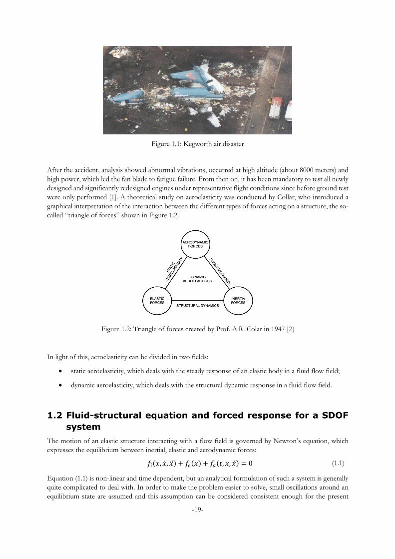
Figure 1.1: Kegworth air disaster
After the accident, analysis showed abnormal vibrations, occurred at high altitude (about 8000 meters) and
high power, which led the fan blade to fatigue failure. From then on, it has been mandatory to test all newly
designed and significantly redesigned engines under representative flight conditions since before ground test
were only performed [1]. A theoretical study on aeroelasticity was conducted by Collar, who introduced a
graphical interpretation of the interaction between the different types of forces acting on a structure, the so-
called “triangle of forces” shown in Figure 1.2.
Figure 1.2: Triangle of forces created by Prof. A.R. Colar in 1947 [2]
In light of this, aeroelasticity can be divided in two fields:
static aeroelasticity, which deals with the steady response of an elastic body in a fluid flow field;
dynamic aeroelasticity, which deals with the structural dynamic response in a fluid flow field.
1.2 Fluid-structural equation and forced response for a SDOF
system
The motion of an elastic structure interacting with a flow field is governed by Newton’s equation, which
expresses the equilibrium between inertial, elastic and aerodynamic forces:
𝑓𝑖(𝑥, �̇�, �̈�) + 𝑓𝑒(𝑥) + 𝑓𝑎(𝑡, 𝑥, �̇�) = 0 (1.1)
Equation (1.1) is non-linear and time dependent, but an analytical formulation of such a system is generally
quite complicated to deal with. In order to make the problem easier to solve, small oscillations around an
equilibrium state are assumed and this assumption can be considered consistent enough for the present
-20-
aeroelastic analysis [1]. Therefore, both structural and aerodynamic terms can be appropriately modelled as
linear so that the equation of motion around the equilibrium state is expressed as:
𝑚�̈� + 𝑐�̇� + 𝑘𝑥 = 𝑓𝑎(𝑡) (1.2)
where m is the mass distribution, c is the damping and k is the stiffness of the solid structure under
consideration. On the right-hand side of equation (1.2), instead, the fluid interaction is modelled by a generic
aerodynamic forcing term 𝑓𝑎(𝑡). In case of forced vibration, this time-varying force has a relevant value
otherwise it is set to zero representing the free vibration case.
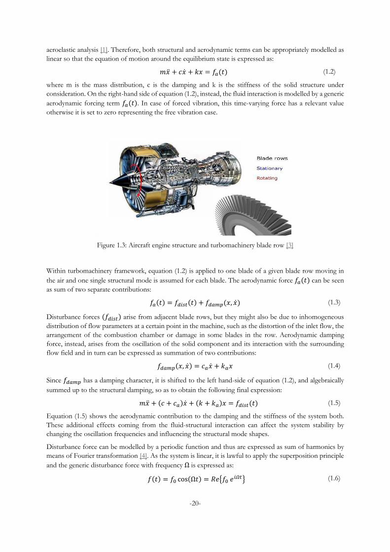
Figure 1.3: Aircraft engine structure and turbomachinery blade row [3]
Within turbomachinery framework, equation (1.2) is applied to one blade of a given blade row moving in
the air and one single structural mode is assumed for each blade. The aerodynamic force 𝑓𝑎(𝑡) can be seen
as sum of two separate contributions:
𝑓𝑎(𝑡) = 𝑓𝑑𝑖𝑠𝑡(𝑡) + 𝑓𝑑𝑎𝑚𝑝(𝑥, �̇�) (1.3)
Disturbance forces (𝑓𝑑𝑖𝑠𝑡) arise from adjacent blade rows, but they might also be due to inhomogeneous
distribution of flow parameters at a certain point in the machine, such as the distortion of the inlet flow, the
arrangement of the combustion chamber or damage in some blades in the row. Aerodynamic damping
force, instead, arises from the oscillation of the solid component and its interaction with the surrounding
flow field and in turn can be expressed as summation of two contributions:
𝑓𝑑𝑎𝑚𝑝(𝑥, �̇�) = 𝑐𝑎�̇� + 𝑘𝑎𝑥 (1.4)
Since 𝑓𝑑𝑎𝑚𝑝 has a damping character, it is shifted to the left hand-side of equation (1.2), and algebraically
summed up to the structural damping, so as to obtain the following final expression:
𝑚�̈� + (𝑐 + 𝑐𝑎)�̇� + (𝑘 + 𝑘𝑎)𝑥 = 𝑓𝑑𝑖𝑠𝑡(𝑡) (1.5)
Equation (1.5) shows the aerodynamic contribution to the damping and the stiffness of the system both.
These additional effects coming from the fluid-structural interaction can affect the system stability by
changing the oscillation frequencies and influencing the structural mode shapes.
Disturbance force can be modelled by a periodic function and thus are expressed as sum of harmonics by
means of Fourier transformation [4]. As the system is linear, it is lawful to apply the superposition principle
and the generic disturbance force with frequency Ω is expressed as:
𝑓(𝑡) = 𝑓0 cos(Ω𝑡) = 𝑅𝑒{𝑓0 𝑒𝑖𝛺𝑡} (1.6)
-21-
where 𝑅𝑒 is the real part of the force, assuming a complex domain. Rewriting equation (1.2) in frequency
domain one can obtain the following expression:
𝑚�̈� + 𝑐�̇� + 𝑘𝑥 = 𝑓0𝑒𝑖Ω𝑡 (1.7)
The particular integral of this differential equation (1.7) is:
𝑥 = 𝑋𝑒𝑖Ω𝑡 (1.8)
where 𝑋 is a complex constant. By computing the first and the second derivative of equation (1.8) and
plugging the derivatives in equation (1.7), the expression of 𝑋 can be found:
𝑋 =
𝑓0𝑘 −𝑚Ω2 + 𝑖Ω𝑐
= 𝐴𝑒𝑖(Ω𝑡+ϕ) (1.9)
where 𝐴 is the amplitude of the motion and 𝜙 is the initial phase, which can be drawn up as follows:
{
𝐴 =
(𝑓0/𝑘)
√(1 − 𝑟2)2 + (2𝜁𝑟)2
𝑡𝑔𝜙 = −2𝜁𝑟
1 − 𝑟2
(1.10)
where 𝑟 =Ω
𝜔𝑛 is the frequency ratio and 𝜁 =
𝑐
2√𝑘𝑚 is the damping ratio.
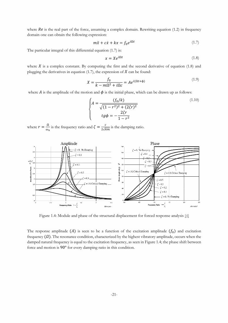
Figure 1.4: Module and phase of the structural displacement for forced response analysis [4]
The response amplitude (𝐴) is seen to be a function of the excitation amplitude (𝑓0) and excitation
frequency (𝛺). The resonance condition, characterized by the highest vibratory amplitude, occurs when the
damped natural frequency is equal to the excitation frequency, as seen in Figure 1.4; the phase shift between
force and motion is 90° for every damping ratio in this condition.
-22-
1.3 Modal analysis and forced response for a MDOF system
The previous motion equation is obtained for a system with one single degree of freedom (SDOF) oscillating
in one direction with a certain natural frequency (𝜔𝑛 = √𝑘/𝑚). However, every vibrating solid body has
more directions of motion and corresponding natural frequencies, which determine the structural mode
shapes. Therefore, it is possible to resort to a discrete system model by assuming multiple degrees of
freedom (MDOF), often used as simplified model for continuous systems. Here again, by combining the
structural equations with the ones coming from the unsteady fluid dynamics [1], the following expression is
obtained in its compact form:
[𝑀]�̈�(𝑡) + [𝐶]�̇�(𝑡) + [𝐾]𝑞(𝑡) = 𝐹(𝑡) (1.11)
where the matrix terms refer to mass, damping and stiffness, while q is conceived as the generalized
displacement vector. 𝐹(𝑡) refers, instead, to the generalized forces vector and acts as connection between
structural dynamics, inertial forces and unsteady aerodynamics. For turbomachinery applications, the two
main components prone to vibrate are disk and blade. Oscillation modes for blades and disks can be
obtained by a structural FEM analysis. The approach used to find these structural deformations is called
modal analysis. In order to perform the latter one it is necessary to set to zero all damping and disturbance
force terms. Hence the simplified expression in this case is:
[𝑀]�̈�(𝑡) + [𝐾]𝑞(𝑡) = 0 (1.12)
where 𝑞(𝑡) = 𝑄𝑒𝑖𝜔𝑡and thus it is possible to pass to frequency domain and define the following
eigenproblem:
(−[𝑀]𝜔2 + [𝐾])𝑄 = 0 (1.13)
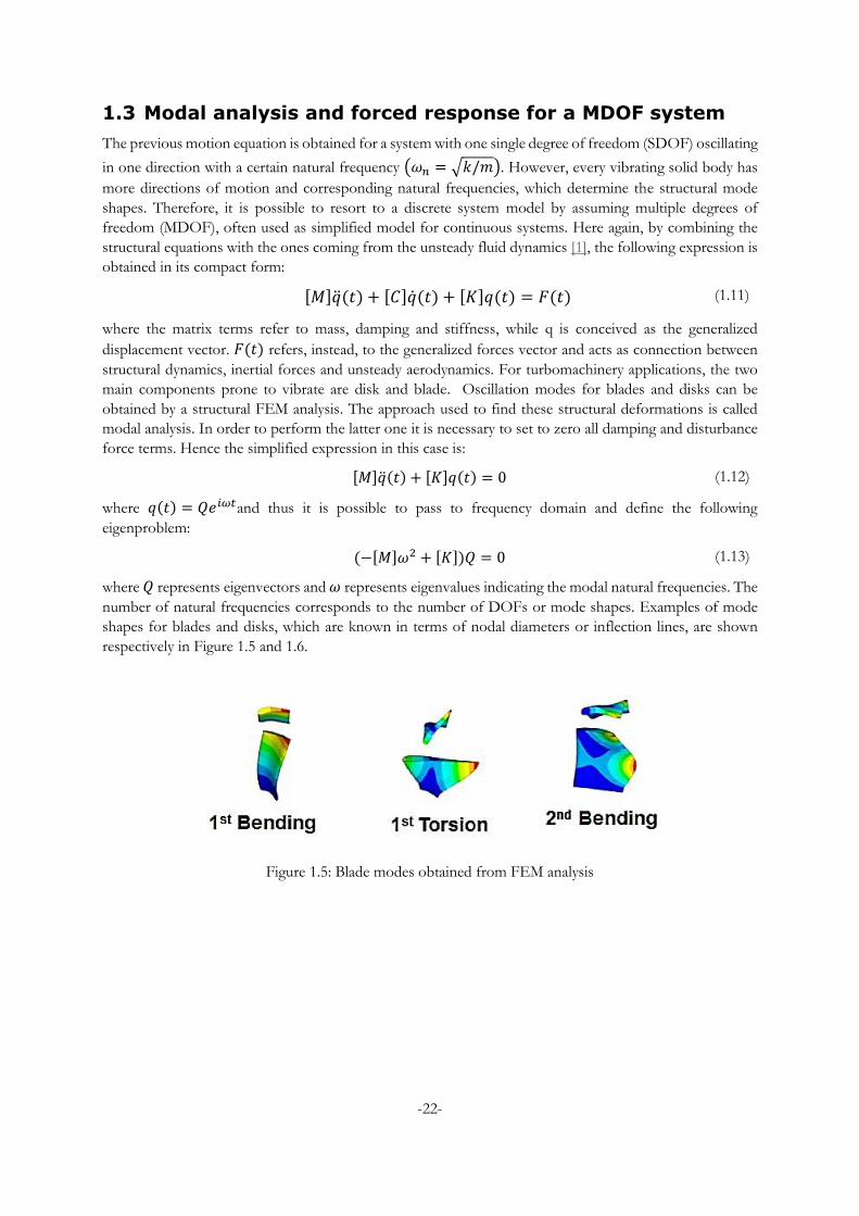
where 𝑄 represents eigenvectors and 𝜔 represents eigenvalues indicating the modal natural frequencies. The
number of natural frequencies corresponds to the number of DOFs or mode shapes. Examples of mode
shapes for blades and disks, which are known in terms of nodal diameters or inflection lines, are shown
respectively in Figure 1.5 and 1.6.
Figure 1.5: Blade modes obtained from FEM analysis
-23-
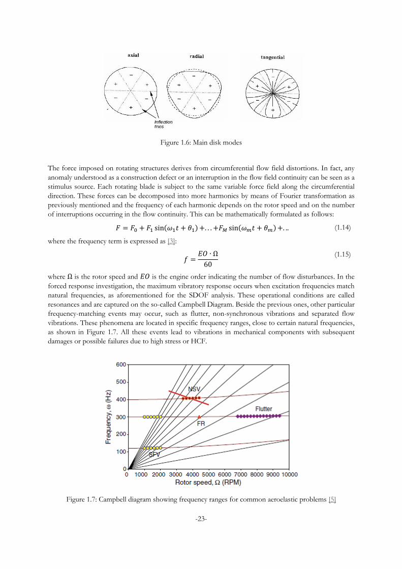
Figure 1.6: Main disk modes
The force imposed on rotating structures derives from circumferential flow field distortions. In fact, any
anomaly understood as a construction defect or an interruption in the flow field continuity can be seen as a
stimulus source. Each rotating blade is subject to the same variable force field along the circumferential
direction. These forces can be decomposed into more harmonics by means of Fourier transformation as
previously mentioned and the frequency of each harmonic depends on the rotor speed and on the number
of interruptions occurring in the flow continuity. This can be mathematically formulated as follows:
𝐹 = 𝐹0 + 𝐹1 sin(𝜔1𝑡 + 𝜃1)+. . . +𝐹𝑀 sin(𝜔𝑚𝑡 + 𝜃𝑚)+. .. (1.14)
where the frequency term is expressed as [3]:
𝑓 =
𝐸𝑂 ∙ Ω
60
(1.15)
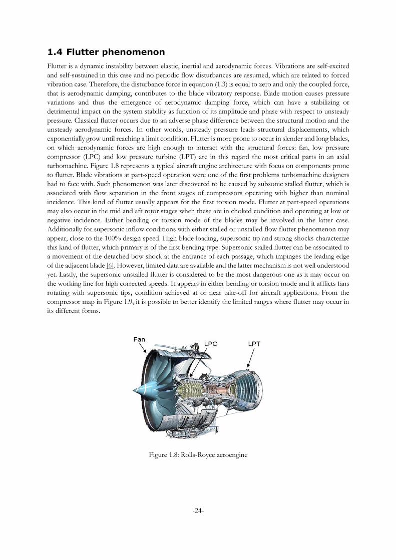
where Ω is the rotor speed and 𝐸𝑂 is the engine order indicating the number of flow disturbances. In the
forced response investigation, the maximum vibratory response occurs when excitation frequencies match
natural frequencies, as aforementioned for the SDOF analysis. These operational conditions are called
resonances and are captured on the so-called Campbell Diagram. Beside the previous ones, other particular
frequency-matching events may occur, such as flutter, non-synchronous vibrations and separated flow
vibrations. These phenomena are located in specific frequency ranges, close to certain natural frequencies,
as shown in Figure 1.7. All these events lead to vibrations in mechanical components with subsequent
damages or possible failures due to high stress or HCF.
Figure 1.7: Campbell diagram showing frequency ranges for common aeroelastic problems [5]
-24-
1.4 Flutter phenomenon
Flutter is a dynamic instability between elastic, inertial and aerodynamic forces. Vibrations are self-excited
and self-sustained in this case and no periodic flow disturbances are assumed, which are related to forced
vibration case. Therefore, the disturbance force in equation (1.3) is equal to zero and only the coupled force,
that is aerodynamic damping, contributes to the blade vibratory response. Blade motion causes pressure
variations and thus the emergence of aerodynamic damping force, which can have a stabilizing or
detrimental impact on the system stability as function of its amplitude and phase with respect to unsteady
pressure. Classical flutter occurs due to an adverse phase difference between the structural motion and the
unsteady aerodynamic forces. In other words, unsteady pressure leads structural displacements, which
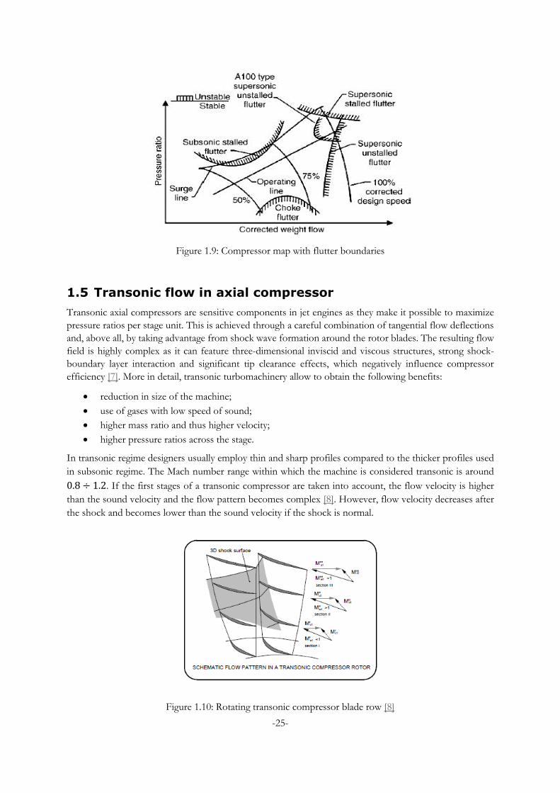
exponentially grow until reaching a limit condition. Flutter is more prone to occur in slender and long blades,
on which aerodynamic forces are high enough to interact with the structural forces: fan, low pressure
compressor (LPC) and low pressure turbine (LPT) are in this regard the most critical parts in an axial
turbomachine. Figure 1.8 represents a typical aircraft engine architecture with focus on components prone
to flutter. Blade vibrations at part-speed operation were one of the first problems turbomachine designers
had to face with. Such phenomenon was later discovered to be caused by subsonic stalled flutter, which is
associated with flow separation in the front stages of compressors operating with higher than nominal
incidence. This kind of flutter usually appears for the first torsion mode. Flutter at part-speed operations
may also occur in the mid and aft rotor stages when these are in choked condition and operating at low or
negative incidence. Either bending or torsion mode of the blades may be involved in the latter case.
Additionally for supersonic inflow conditions with either stalled or unstalled flow flutter phenomenon may
appear, close to the 100% design speed. High blade loading, supersonic tip and strong shocks characterize
this kind of flutter, which primary is of the first bending type. Supersonic stalled flutter can be associated to
a movement of the detached bow shock at the entrance of each passage, which impinges the leading edge
of the adjacent blade [6]. However, limited data are available and the latter mechanism is not well understood
yet. Lastly, the supersonic unstalled flutter is considered to be the most dangerous one as it may occur on
the working line for high corrected speeds. It appears in either bending or torsion mode and it afflicts fans
rotating with supersonic tips, condition achieved at or near take-off for aircraft applications. From the
compressor map in Figure 1.9, it is possible to better identify the limited ranges where flutter may occur in
its different forms.
Figure 1.8: Rolls-Royce aeroengine
-25-
Figure 1.9: Compressor map with flutter boundaries
1.5 Transonic flow in axial compressor
Transonic axial compressors are sensitive components in jet engines as they make it possible to maximize
pressure ratios per stage unit. This is achieved through a careful combination of tangential flow deflections
and, above all, by taking advantage from shock wave formation around the rotor blades. The resulting flow
field is highly complex as it can feature three-dimensional inviscid and viscous structures, strong shock-
boundary layer interaction and significant tip clearance effects, which negatively influence compressor
efficiency [7]. More in detail, transonic turbomachinery allow to obtain the following benefits:
reduction in size of the machine;
use of gases with low speed of sound;
higher mass ratio and thus higher velocity;
higher pressure ratios across the stage.
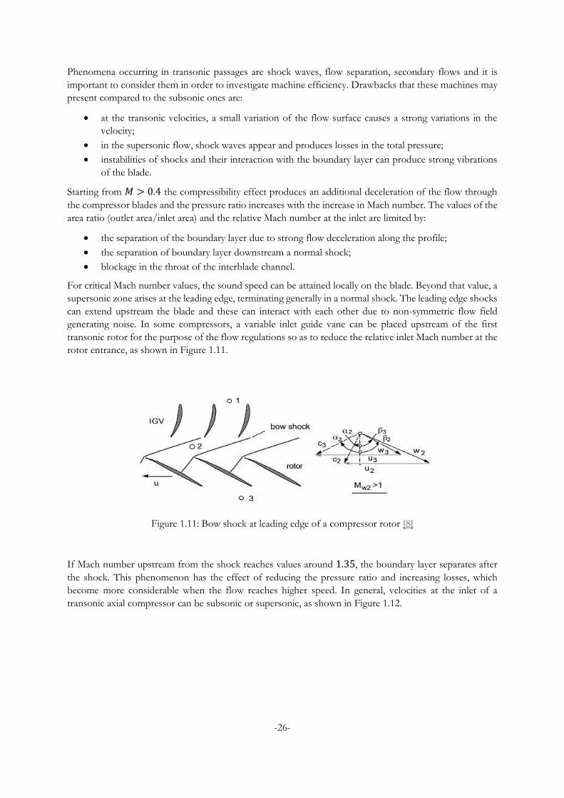
In transonic regime designers usually employ thin and sharp profiles compared to the thicker profiles used
in subsonic regime. The Mach number range within which the machine is considered transonic is around
0.8 ÷ 1.2. If the first stages of a transonic compressor are taken into account, the flow velocity is higher
than the sound velocity and the flow pattern becomes complex [8]. However, flow velocity decreases after
the shock and becomes lower than the sound velocity if the shock is normal.
Figure 1.10: Rotating transonic compressor blade row [8]
-26-
Phenomena occurring in transonic passages are shock waves, flow separation, secondary flows and it is
important to consider them in order to investigate machine efficiency. Drawbacks that these machines may
present compared to the subsonic ones are:
at the transonic velocities, a small variation of the flow surface causes a strong variations in the
velocity;
in the supersonic flow, shock waves appear and produces losses in the total pressure;
instabilities of shocks and their interaction with the boundary layer can produce strong vibrations
of the blade.
Starting from 𝑀 > 0.4 the compressibility effect produces an additional deceleration of the flow through
the compressor blades and the pressure ratio increases with the increase in Mach number. The values of the
area ratio (outlet area/inlet area) and the relative Mach number at the inlet are limited by:
the separation of the boundary layer due to strong flow deceleration along the profile;
the separation of boundary layer downstream a normal shock;
blockage in the throat of the interblade channel.
For critical Mach number values, the sound speed can be attained locally on the blade. Beyond that value, a
supersonic zone arises at the leading edge, terminating generally in a normal shock. The leading edge shocks
can extend upstream the blade and these can interact with each other due to non-symmetric flow field
generating noise. In some compressors, a variable inlet guide vane can be placed upstream of the first
transonic rotor for the purpose of the flow regulations so as to reduce the relative inlet Mach number at the
rotor entrance, as shown in Figure 1.11.
Figure 1.11: Bow shock at leading edge of a compressor rotor [8]
If Mach number upstream from the shock reaches values around 1.35, the boundary layer separates after
the shock. This phenomenon has the effect of reducing the pressure ratio and increasing losses, which
become more considerable when the flow reaches higher speed. In general, velocities at the inlet of a
transonic axial compressor can be subsonic or supersonic, as shown in Figure 1.12.
-27-
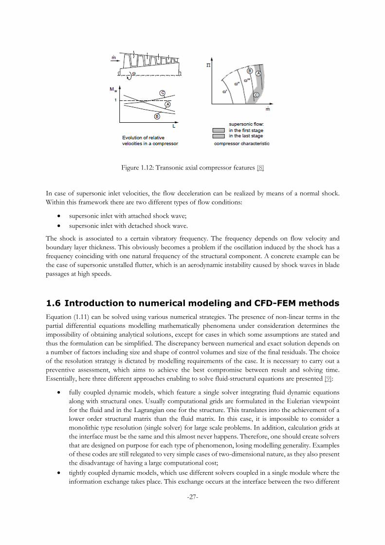
Figure 1.12: Transonic axial compressor features [8]
In case of supersonic inlet velocities, the flow deceleration can be realized by means of a normal shock.
Within this framework there are two different types of flow conditions:
supersonic inlet with attached shock wave;
supersonic inlet with detached shock wave.
The shock is associated to a certain vibratory frequency. The frequency depends on flow velocity and
boundary layer thickness. This obviously becomes a problem if the oscillation induced by the shock has a
frequency coinciding with one natural frequency of the structural component. A concrete example can be
the case of supersonic unstalled flutter, which is an aerodynamic instability caused by shock waves in blade
passages at high speeds.
1.6 Introduction to numerical modeling and CFD-FEM methods
Equation (1.11) can be solved using various numerical strategies. The presence of non-linear terms in the
partial differential equations modelling mathematically phenomena under consideration determines the
impossibility of obtaining analytical solutions, except for cases in which some assumptions are stated and
thus the formulation can be simplified. The discrepancy between numerical and exact solution depends on
a number of factors including size and shape of control volumes and size of the final residuals. The choice
of the resolution strategy is dictated by modelling requirements of the case. It is necessary to carry out a
preventive assessment, which aims to achieve the best compromise between result and solving time.
Essentially, here three different approaches enabling to solve fluid-structural equations are presented [9]:
fully coupled dynamic models, which feature a single solver integrating fluid dynamic equations
along with structural ones. Usually computational grids are formulated in the Eulerian viewpoint
for the fluid and in the Lagrangian one for the structure. This translates into the achievement of a
lower order structural matrix than the fluid matrix. In this case, it is impossible to consider a
monolithic type resolution (single solver) for large scale problems. In addition, calculation grids at
the interface must be the same and this almost never happens. Therefore, one should create solvers
that are designed on purpose for each type of phenomenon, losing modelling generality. Examples
of these codes are still relegated to very simple cases of two-dimensional nature, as they also present
the disadvantage of having a large computational cost;
tightly coupled dynamic models, which use different solvers coupled in a single module where the
information exchange takes place. This exchange occurs at the interface between the two different

-28-
computational grids. The fluid-dynamic solver provides the force values to the structural one, which
in turn communicates the displacements. Computational grids are thus moving and this implies that
there is also the development of algorithms enabling to modify or reconstruct a new mesh. In this
large family of solvers, the implemented equations of fluid dynamics can range from the simple
potential flow equation up to the use of RANS equations. On the structural side, both the beam
model and the non-linear solid element can be implemented;
decoupled dynamic models, in which the two environments are solved by separate solvers and thus
computational grids can be different, structured, hybrid and non-compliant. In this case, an
information exchange interface must be developed. The information exchange is partial and there
are only external interactions between the two environments. This method is useful for more simple
applications because it loses accuracy in more complex cases. One of the advantages for which
these methods are still used lies in the flexibility of use; in fact, it is possible to choose any
computational grid or the solver more appropriate for each environment as function of the
application.
In the present work, the latter strategy has been used since structural forces can be considered higher
than aerodynamic forces for turbomachinery applications and this allow to decouple the interaction
between fluid and structure. Therefore, it has been possible to investigate only the fluid environment,
while structural displacements were obtained from previous studies not included in this work.
-29-
2 THEORETICAL APPROACH
One direct consequence of unsteady flow fluctuations is the appearance of aerodynamic damping, which is
a parameter of paramount importance in an aeroelastic analysis. Aerodynamic damping denotes the part of
damping arising from the flow around structural components and differs from the structural damping,
which depends on blade structural properties. Aerodynamic stiffness appears also due to the aerodynamics
around the blades and is summed up along with the structural stiffness. It is necessary to evaluate this
parameter during turbine, compressor and fan designs to predict structural vibrations and estimate blade
life. This work investigates aerodynamic damping in transonic axial compressor blades with focus on
different mode shapes.
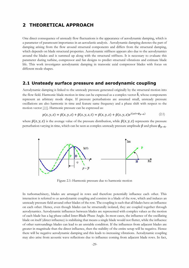
2.1 Unsteady surface pressure and aerodynamic coupling
Aerodynamic damping is linked to the unsteady pressure generated originally by the structural motion into
the flow field. Harmonic blade motion in time can be expressed as a complex vector ℎ̂, whose components
represent an arbitrary mode shape. If pressure perturbations are assumed small, unsteady pressure
oscillations are also harmonic in time and feature same frequency and a phase shift with respect to the
motion vector [10]. Harmonic pressure can be expressed as:
𝑝(𝑥, 𝑦, 𝑧) = �̅�(𝑥, 𝑦, 𝑧) + �̃�(𝑥, 𝑦, 𝑧, 𝑡) = �̅�(𝑥, 𝑦, 𝑧) + �̂�(𝑥, 𝑦, 𝑧)𝑒𝑖(𝜔𝑡+𝜙𝑝→ℎ) (2.1)
where �̅�(𝑥, 𝑦, 𝑧) is the average value of the pressure distribution, while �̃�(𝑥, 𝑦, 𝑧) represents the pressure
perturbation varying in time, which can be seen as complex unsteady pressure amplitude �̂� and phase 𝜙𝑝→ℎ.
Figure 2.1: Harmonic pressure due to harmonic motion
In turbomachinery, blades are arranged in rows and therefore potentially influence each other. This
interaction is referred to as aerodynamic coupling and consists in a blade of the row, which and induces an
unsteady pressure field around other blades of the row. The coupling is such that all blades have an influence
on each other. Hence, even though blades can be structurally isolated, they are coupled together through
aerodynamics. Aerodynamic influences between blades are represented with complex values as the motion
of each blade has a lag phase called Inter-Blade Phase Angle. In most cases, the influence of the oscillating
blade on itself (direct influence) is stabilizing that means a single blade would not flutter, while the influence
of other surroundings blades can lead to an unstable condition. If the influences from adjacent blades are
greater in magnitude than the direct influence, then the stability of the entire setup will be negative. Hence
there will be negative aerodynamic damping and this leads to increasing vibrations. Aerodynamic coupling
may also arise from acoustic wave reflections due to influence coming from adjacent blade rows. In fact,
-30-
upstream or downstream blade rows might receive an acoustic wave from the blade row under consideration
and the subsequent reflection waves can affect system stability. This effect is neglected in the present work
by using non-reflective boundary condition at the inlet and outlet interfaces, particularly needed for cut-on
frequency configurations [11].
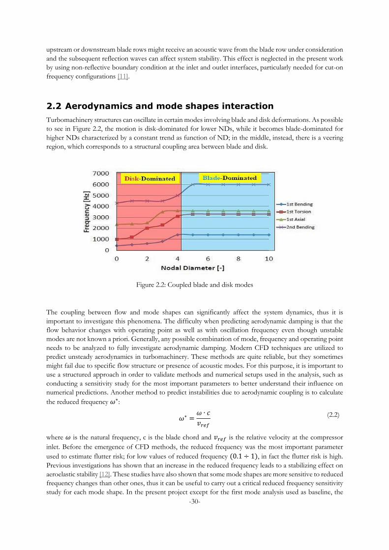
2.2 Aerodynamics and mode shapes interaction
Turbomachinery structures can oscillate in certain modes involving blade and disk deformations. As possible
to see in Figure 2.2, the motion is disk-dominated for lower NDs, while it becomes blade-dominated for
higher NDs characterized by a constant trend as function of ND; in the middle, instead, there is a veering
region, which corresponds to a structural coupling area between blade and disk.
Figure 2.2: Coupled blade and disk modes
The coupling between flow and mode shapes can significantly affect the system dynamics, thus it is
important to investigate this phenomena. The difficulty when predicting aerodynamic damping is that the
flow behavior changes with operating point as well as with oscillation frequency even though unstable
modes are not known a priori. Generally, any possible combination of mode, frequency and operating point
needs to be analyzed to fully investigate aerodynamic damping. Modern CFD techniques are utilized to
predict unsteady aerodynamics in turbomachinery. These methods are quite reliable, but they sometimes
might fail due to specific flow structure or presence of acoustic modes. For this purpose, it is important to
use a structured approach in order to validate methods and numerical setups used in the analysis, such as
conducting a sensitivity study for the most important parameters to better understand their influence on
numerical predictions. Another method to predict instabilities due to aerodynamic coupling is to calculate
the reduced frequency 𝜔∗:
𝜔∗ =
𝜔 ∙ 𝑐
𝑣𝑟𝑒𝑓
(2.2)
where 𝜔 is the natural frequency, c is the blade chord and 𝑣𝑟𝑒𝑓 is the relative velocity at the compressor
inlet. Before the emergence of CFD methods, the reduced frequency was the most important parameter
used to estimate flutter risk; for low values of reduced frequency (0.1 ÷ 1), in fact the flutter risk is high.
Previous investigations has shown that an increase in the reduced frequency leads to a stabilizing effect on
aeroelastic stability [12]. These studies have also shown that some mode shapes are more sensitive to reduced
frequency changes than other ones, thus it can be useful to carry out a critical reduced frequency sensitivity
study for each mode shape. In the present project except for the first mode analysis used as baseline, the
-31-
other modes feature reduced frequency values out of the critical range, thus the flutter risk is not significant.
A graphical method developed to assess aerodynamic stability on a two dimensional section is called mode
shape sensitivity plot [13]. This method is based on representing any possible pure rigid body mode as
torsion mode around a respective center of torsion in order to determine the critical reduced frequency for
different structural modes, as possible to see in Figure 2.3.
Figure 2.3: Stability plots, also called tie-dye plots [14]
2.3 Theoretical methods for aerodamping predictions
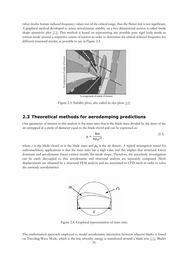
One parameter of interest in this analysis is the mass ratio that is the blade mass divided by the mass of the
air entrapped in a circle of diameter equal to the blade chord and can be expressed as:
𝜇 =
4𝑚
𝜋𝜌0𝑐2
(2.3)
where c is the blade chord, m is the blade mass and 𝜌0 is the air density. A typical assumption stated for
turbomachinery applications is that the mass ratio has a high value and this implies that structural forces
dominate and aerodynamic forces cannot modify the mode shape. Therefore, the aeroelastic investigation
can be easily decoupled so that aerodynamic and structural analysis are separately computed. Mesh
displacements are obtained by a structural FEM analysis and are associated to CFD mesh in order to solve
the unsteady aerodynamics.
Figure 2.4: Graphical representation of mass ratio
The mathematical approach employed to model aerodynamic interaction between adjacent blades is based
on Traveling Wave Mode, which is the way whereby energy is transferred around a blade row [15]. Blades
-32-
are assumed tuned that means every blade of the row is supposed to have exactly the same structural and
material properties (same stiffness and density). In reality, blades are not equal to each other due to
manufacturing tolerances or different wear during operations thus they can be defined randomly mistuned.
A supplementary effect can be added by intentional mistuning consisting in varying the blade natural
frequency by some percentage order in a certain mistuning pattern. This helps to break the TWM in case of
flutter, while it may increase oscillation amplitude in case of forced response and lead to more severe
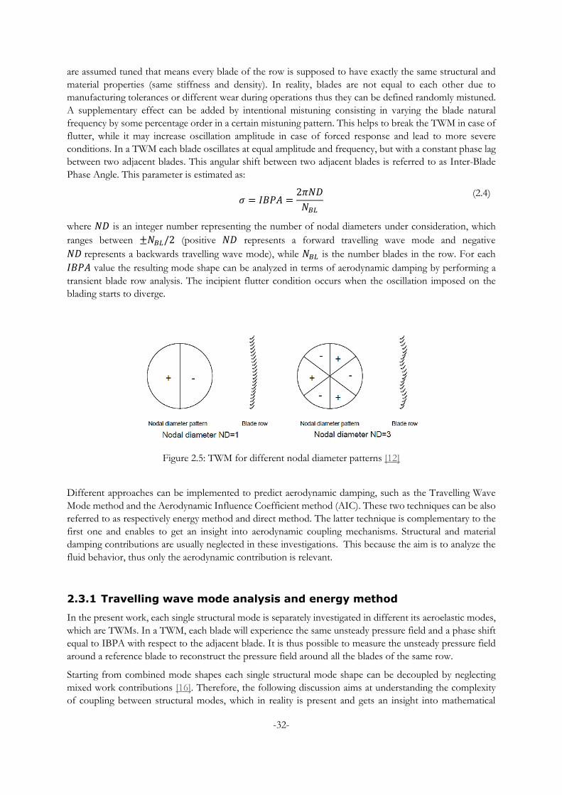
conditions. In a TWM each blade oscillates at equal amplitude and frequency, but with a constant phase lag
between two adjacent blades. This angular shift between two adjacent blades is referred to as Inter-Blade
Phase Angle. This parameter is estimated as:
𝜎 = 𝐼𝐵𝑃𝐴 =
2𝜋𝑁𝐷
𝑁𝐵𝐿
(2.4)
where 𝑁𝐷 is an integer number representing the number of nodal diameters under consideration, which
ranges between ±𝑁𝐵𝐿/2 (positive 𝑁𝐷 represents a forward travelling wave mode and negative
𝑁𝐷 represents a backwards travelling wave mode), while 𝑁𝐵𝐿 is the number blades in the row. For each
𝐼𝐵𝑃𝐴 value the resulting mode shape can be analyzed in terms of aerodynamic damping by performing a
transient blade row analysis. The incipient flutter condition occurs when the oscillation imposed on the
blading starts to diverge.
Figure 2.5: TWM for different nodal diameter patterns [12]
Different approaches can be implemented to predict aerodynamic damping, such as the Travelling Wave
Mode method and the Aerodynamic Influence Coefficient method (AIC). These two techniques can be also
referred to as respectively energy method and direct method. The latter technique is complementary to the
first one and enables to get an insight into aerodynamic coupling mechanisms. Structural and material
damping contributions are usually neglected in these investigations. This because the aim is to analyze the
fluid behavior, thus only the aerodynamic contribution is relevant.
2.3.1 Travelling wave mode analysis and energy method
In the present work, each single structural mode is separately investigated in different its aeroelastic modes,
which are TWMs. In a TWM, each blade will experience the same unsteady pressure field and a phase shift
equal to IBPA with respect to the adjacent blade. It is thus possible to measure the unsteady pressure field
around a reference blade to reconstruct the pressure field around all the blades of the same row.
Starting from combined mode shapes each single structural mode shape can be decoupled by neglecting
mixed work contributions [16]. Therefore, the following discussion aims at understanding the complexity
of coupling between structural modes, which in reality is present and gets an insight into mathematical
-33-
workaround addressing to split contributions up. After knowing the unsteady aerodynamics for each mode
and blade motion, the energy method can be applied for the evaluation of aerodynamic damping.
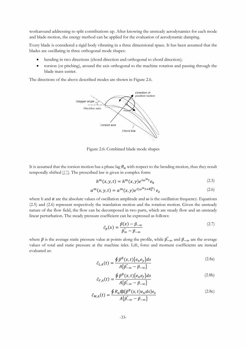
Every blade is considered a rigid body vibrating in a three dimensional space. It has been assumed that the
blades are oscillating in three orthogonal mode shapes:
bending in two directions (chord direction and orthogonal to chord direction);
torsion (or pitching), around the axis orthogonal to the machine rotation and passing through the
blade mass center.
The directions of the above described modes are shown in Figure 2.6.
Figure 2.6: Combined blade mode shapes
It is assumed that the torsion motion has a phase lag 𝜃𝑎 with respect to the bending motion, thus they result
temporally shifted [17]. The prescribed law is given in complex form:
ℎ𝑚(𝑥, 𝑦, 𝑡) = ℎ𝑚(𝑥, 𝑦)𝑒𝑖𝜔𝑚𝑡𝑒ℎ (2.5)
𝛼𝑚(𝑥, 𝑦, 𝑡) = 𝛼𝑚(𝑥, 𝑦)𝑒𝑖(𝜔𝑚𝑡+𝜃𝑎
𝑚) 𝑒𝑧 (2.6)
where h and 𝛼 are the absolute values of oscillation amplitude and 𝜔 is the oscillation frequency. Equations
(2.5) and (2.6) represent respectively the translation motion and the rotation motion. Given the unsteady
nature of the flow field, the flow can be decomposed in two parts, which are steady flow and an unsteady
linear perturbation. The steady pressure coefficient can be expressed as follows:
𝑐�̅�(𝑥) =
�̅�(𝑥) − �̅�−∞
�̅�∞° − �̅�−∞
(2.7)
where �̅� is the average static pressure value at points along the profile, while �̅�−∞° and �̅�−∞ are the average
values of total and static pressure at the machine inlet. Lift, force and moment coefficients are instead
evaluated as:
�̃�𝐿,𝐴(𝑡) =
∮ �̃�𝐵(𝑥, 𝑡){𝑒𝑛𝑒𝑦}𝑑𝑠
𝐴{�̅�−∞° − �̅�−∞}
(2.8a)
�̃�𝐹,𝐴(𝑡) =
∮ �̃�𝐵(𝑥, 𝑡){𝑒𝑛𝑒𝑓}𝑑𝑠
𝐴{�̅�−∞° − �̅�−∞}
(2.8b)
�̃�𝑀,𝐴(𝑡) =
∮𝑅𝑎⨂{�̃�𝐵(𝑥, 𝑡)𝑒𝑛𝑑𝑠}𝑒𝑧
𝐴{�̅�−∞° − �̅�−∞}
(2.8c)
-34-
where �̃�𝐵is the unsteady pressure amplitude and 𝑅𝑎 is the radius vector. The reference surface is denoted
by apex 𝐵, which may be the suction or pressure side of the blade profile. The lift coefficient is calculated
in the direction orthogonal to the blade chord (𝑒𝑦), while the force coefficient in the chord direction (𝑒𝑓).
The unit vector 𝑒𝑛 is orthogonal to the blade profile and the integration step ds is the distance between two
adjacent points describing the profile curve. It is possible to notice that all the previous coefficients are
normalized by using the non-dimensional parameter A:
A=𝐴𝑚
𝑐 (2.9)
where 𝑐 is the chord and 𝐴𝑚 is the prescribed displacement amplitude. The unsteady pressure coefficient
can be now introduced [12]:
�̃�𝑝,𝐴𝐵 (𝑥, 𝑡) =
�̃�𝐵(𝑥, 𝑡)
𝐴(�̅�°−∞ − �̅�−∞)
(2.10)
It is thus possible to substitute equation (2.10) in equations (2.8) so as to obtain expressions as function of
the unsteady pressure coefficient. The global pressure coefficient can be expressed as the summation of
the steady pressure coefficient in time and the unsteady pressure coefficient:
�̃�𝑝𝑔𝑙𝑜𝑏𝑎𝑙(𝑥, 𝑡) = 𝑐�̅�(𝑥) + 𝐴�̃�𝑝(𝑥, 𝑡) =
{�̅� − �̅�−∞} + �̃�𝐵(𝑥, 𝑦)
{�̅�°−∞ − �̅�−∞}
(2.11)
The unsteady pressure coefficient in time domain can be transferred to frequency domain by means of
Fourier transformation in order to reduce solving efforts:
�̃�𝑝(𝑥, 𝑡) = �̃�𝑝(𝑥)𝑒𝜔𝑡+𝜙𝑝(𝑥) = �̃�𝑝(𝑥)𝑒
𝑖𝜔𝑡𝑒𝜙𝑝(𝑥) = �̂�𝑝𝑐𝑜𝑚𝑝𝑙𝑒𝑥(𝑥)𝑒𝑖𝜔𝑡
= (𝑅𝑒{�̂�𝑝𝑐𝑜𝑚𝑝𝑙𝑒𝑥(𝑥)} + 𝐼𝑚{�̂�𝑝
𝑐𝑜𝑚𝑝𝑙𝑒𝑥(𝑥)})𝑒𝑖𝜔𝑡
(2.12)
where 𝑅𝑒 and 𝐼𝑚 are real and imaginary component of the pressure coefficient. The real component is in
phase with the harmonic motion, while the imaginary part is out of phase. The two-dimensional
aerodynamic work per height unit performed by aerodynamic forces and moments on the blade, considered
as a rigid body, is conventionally expressed by the product of the real part of the force, or the moment, and
respectively of the real part of translation, or torsion of the body:
�̃�𝑤,ℎ=∫𝑅𝑒{ℎ(𝑥,𝑦,𝑧)𝑐̃ℎ(𝑡)}𝑅𝑒{𝑑ℎ(𝑥,𝑦,𝑡)} (2.13a)
�̃�𝑤,ℎ=∫𝑅𝑒{𝛼(𝑡)𝑐�̃�(𝑡)}𝑅𝑒{𝑑𝛼(𝑡)} (2.13b)
�̃�𝑤,ℎ,𝛼=∫𝑅𝑒{ℎ(𝑥,𝑦,𝑧)𝑐̃𝑚,ℎ(𝑡)}𝑅𝑒{𝑑𝛼(𝑡)} (2.13c)
�̃�𝑤,ℎ=∫𝑅𝑒{𝛼(𝑡)𝑐�̃�,𝛼(𝑡)}𝑅𝑒{𝑑ℎ(𝑥,𝑦,𝑡)} (2.13d)
where the first two terms of equations (2.13) represent the pure works, which are bending and torsional
work, while the last two terms represent the mixed work contributions. The total work can be then calculated
by summing up the four contributions, as shown in the equation below:
�̃�𝑤 = �̃�𝑤,ℎ + �̃�𝑤,𝛼 + �̃�𝑤,ℎ,𝛼 + �̃�𝑤,𝛼,ℎ (2.14)
If now the degrees of freedom are decoupled, only pure bending and pure torsional work survive. By
integrating the previous expressions one can obtain:
�̃�𝑤,ℎ = 𝜋ℎ2𝐼𝑚{�̃�ℎ
𝑐𝑜𝑚𝑝𝑙𝑒𝑥} = 𝜋ℎ2�̃�ℎ𝑠𝑖𝑛𝜙ℎ (2.15a)
�̃�𝑤,𝛼 = 𝜋ℎ2𝐼𝑚{�̃�ℎ
𝑐𝑜𝑚𝑝𝑙𝑒𝑥} = 𝜋ℎ2�̃�𝑀𝑠𝑖𝑛𝜙𝑀 (2.15b)
�̃�𝑤,ℎ,𝛼 = 0 (2.15c)
-35-
�̃�𝑤,𝛼,ℎ = 0 (2.15d)
It can be seen from equations (2.15) that aerodynamic work depends only on the phase of the force or
moment coefficient. Aerodynamic work can be normalized and this allows to obtain the expression of
aerodynamic damping coefficients for bending and torsion mode:
Θℎ = −
�̃�𝑤,ℎ𝜋ℎ2
(2.16a)
Θ𝛼 = −
�̃�𝑤,𝛼𝜋𝛼2
(2.16b)
This value is positive when the flow dampens blade vibration, while it is negative when the fluid gives energy
to the blade.
Energy method directly assumes one degree of freedom for each blade and high mass ratio enabling to
decouple the fluid dynamics from the structural dynamics. A simplified formulation of the unsteady work
per cycle [2] for a single structural mode is written as:
𝑊𝑎𝑒𝑟𝑜 = −∫ 𝜋ℎ ∙ �̅�𝑝𝑖𝑑𝐴
𝐴
(2.17)
where ℎ is the maximum displacement, 𝑝𝑖 is the imaginary component of the pressure and �̅� is the unit
vector normal to the blade surface part considered. Another parameter useful to define in this analysis is
the average kinetic energy of the blade, which has the following final expression:
𝐾𝐸𝑎𝑣𝑒 =
𝜔2
4
(2.18)
This latter formulation is obtained starting from the definition of kinetic energy for a rigid body moving in
a single structural mode:
𝐾𝐸𝑎𝑣𝑒 =
1
2𝑚𝑣2
(2.19)
where 𝑚 is the body mass and 𝑣 is its velocity, which is the derivative of the harmonic motion:
𝑥(𝑡) = �̅�cos (𝜔𝑡) (2.20a)
𝑣(𝑡) = −𝜔�̅�sin (𝜔𝑡) (2.20b)
where since the time-average value of sin2(𝑡) is equal to 1/2, then equation (2.18) can be obtained. For a
given mode, it is possible to get the S-shape curve, which enables to recognize stable and unstable regions.
This curve can be build up by using aerodamping coefficient values as function of the IBPA or evaluating
the logarithmic decrement values for each configuration. The logarithmic decrement is defined as the
relative change in amplitude per cycle and is estimated by the expression below:
𝛿 =
−𝑊𝑎𝑒𝑟𝑜4𝐾𝐸𝑎𝑣𝑒
(2.21)
It is important to evaluate the average kinetic energy of the blade and the aerodynamic work at the same
blade amplitude in order to be consistent in the analysis.
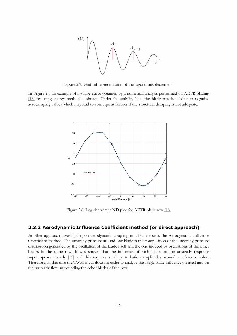
-36-
Figure 2.7: Grafical representation of the logarithmic decrement
In Figure 2.8 an example of S-shape curve obtained by a numerical analysis performed on AETR blading
[18] by using energy method is shown. Under the stability line, the blade row is subject to negative
aerodamping values which may lead to consequent failures if the structural damping is not adequate.
Figure 2.8: Log-dec versus ND plot for AETR blade row [18]
2.3.2 Aerodynamic Influence Coefficient method (or direct approach)
Another approach investigating on aerodynamic coupling in a blade row is the Aerodynamic Influence
Coefficient method. The unsteady pressure around one blade is the composition of the unsteady pressure
distribution generated by the oscillation of the blade itself and the one induced by oscillations of the other
blades in the same row. It was shown that the influence of each blade on the unsteady response
superimposes linearly [15] and this requires small perturbation amplitudes around a reference value.
Therefore, in this case the TWM is cut down in order to analyze the single blade influence on itself and on
the unsteady flow surrounding the other blades of the row.
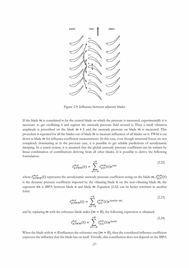
-37-
Figure 2.9: Influence between adjacent blades
If the blade 𝑚 is considered to be the central blade on which the pressure is measured, experimentally it is
necessary to get oscillating it and register the unsteady pressure field around it. Then a small vibration
amplitude is prescribed on the blade 𝑚 + 1 and the unsteady pressure on blade 𝑚 is measured. This
procedure is repeated for all the blades out of blade 𝑚 to measure influences of all blades on it. TWM is cut
down at blade 𝑚 for influence coefficient measurements. In this case, even though structural forces are not
completely dominating as in the previous case, it is possible to get reliable predictions of aerodynamic
damping. In a tuned system, it is assumed that the global unsteady pressure coefficient can be written by
linear combination of contributions deriving from all other blades. It is possible to derive the following
formulation:
�̃�𝑝,𝑇𝑊𝑀𝑚,𝜎 (𝑡) = ∑ �̃�𝑝,𝐼𝐶
𝑛,𝑚(𝑡)𝑒𝑖𝜎𝑛+𝑁
𝑛=−𝑁
(2.22)
where �̃�𝑝,𝑇𝑊𝑀𝑚,𝜎 (𝑡) represents the aerodynamic unsteady pressure coefficient acting on the blade 𝑚, �̃�𝑝,𝐼𝐶
𝑛,𝑚(𝑡)
is the dynamic pressure coefficient imposed by the vibrating blade 𝑛 on the non-vibrating blade 𝑚, the
exponent 𝜎𝑛 is IBPA between blade 𝑛 and blade 𝑚. Equation (2.22) can be better rewritten in another
form:
�̃�𝑝,𝑇𝑊𝑀𝑚,𝜎 (𝑡) = ∑ �̃�𝑝,𝑖𝑐
𝑛,𝑚(𝑡)𝑒𝑖𝜔𝜎(𝑛−𝑚)+𝑁
𝑛=−𝑁
(2.23)
and by replacing 𝑚 with the reference blade index (𝑚 = 0), the following expression is obtained:
�̃�𝑝,𝑇𝑊𝑀0,𝜎 (𝑡) = ∑ �̃�𝑝,𝑖𝑐
𝑛,0 (𝑡)𝑒𝑖𝜔𝜎𝑛+𝑁
𝑛=−𝑁
(2.24)
When the blade with 𝑛 = 0 influences the reference one (𝑚 = 0), then the considered influence coefficient
expresses the influence that the blade has on itself. Trivially, this contribution does not depend on the IBPA
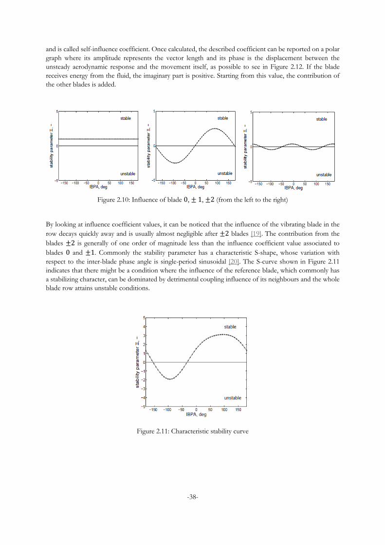
-38-
and is called self-influence coefficient. Once calculated, the described coefficient can be reported on a polar
graph where its amplitude represents the vector length and its phase is the displacement between the
unsteady aerodynamic response and the movement itself, as possible to see in Figure 2.12. If the blade
receives energy from the fluid, the imaginary part is positive. Starting from this value, the contribution of
the other blades is added.
Figure 2.10: Influence of blade 0, ± 1, ±2 (from the left to the right)
By looking at influence coefficient values, it can be noticed that the influence of the vibrating blade in the
row decays quickly away and is usually almost negligible after ±2 blades [19]. The contribution from the
blades ±2 is generally of one order of magnitude less than the influence coefficient value associated to
blades 0 and ±1. Commonly the stability parameter has a characteristic S-shape, whose variation with
respect to the inter-blade phase angle is single-period sinusoidal [20]. The S-curve shown in Figure 2.11
indicates that there might be a condition where the influence of the reference blade, which commonly has
a stabilizing character, can be dominated by detrimental coupling influence of its neighbours and the whole
blade row attains unstable conditions.
Figure 2.11: Characteristic stability curve
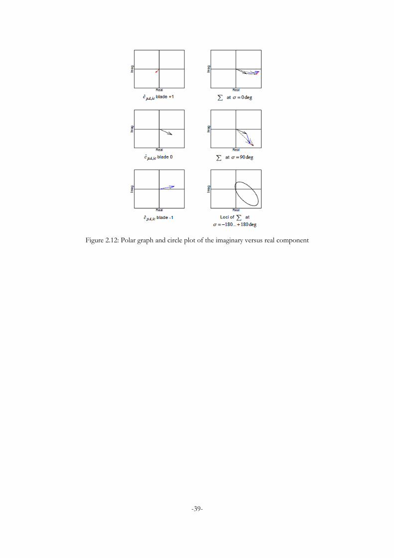
-39-
Figure 2.12: Polar graph and circle plot of the imaginary versus real component

-40-
3 OBJECTIVE
The proposed work herein aims at numerically investigating aerodynamic damping with focus on the first
six mode shapes of the original VINK first rotor blades. Different numerical approaches currently available
in ANSYS CFX software have been compared as well as the influence of several parameters on numerical
predictions has been investigated.
Within the framework of a recently started H2020 project called ARIAS, a new test rig will be established
at KTH. The purpose of the test facility is to generate a unique set of blade surface unsteady pressure data
for validation of prediction models for aerodynamic damping in transonic compressor blades oscillating at
high-reduced frequencies. The blade profile that will be used in the test rig originates from the NFFP6
project called VINK and is a 2D extrusion of a profile extracted at the 95% span of the rotor blades from
the 3-stage high-speed transonic booster.
Based on the findings of the present work, different objectives will be attained:
To broaden knowledge about mode shape sensitivity of VINK first rotor blades, with the main
focus placed on investigations of unsteady surface pressure at different span locations. The
investigation involves only numerical CFD simulations and can be considered as a continuation of
previous aeroelastic studies conducted on the same 3-stage high-speed transonic booster;
To provide useful data and predictions for the development of the oscillating cascade rig;
To recommend the optimum placement of the pressure transducers for measurements of the
aerodynamic response in the oscillating cascade rig;
To get insights into different numerical setups evaluating eventual mismatches with respect to the
successive experimental results.
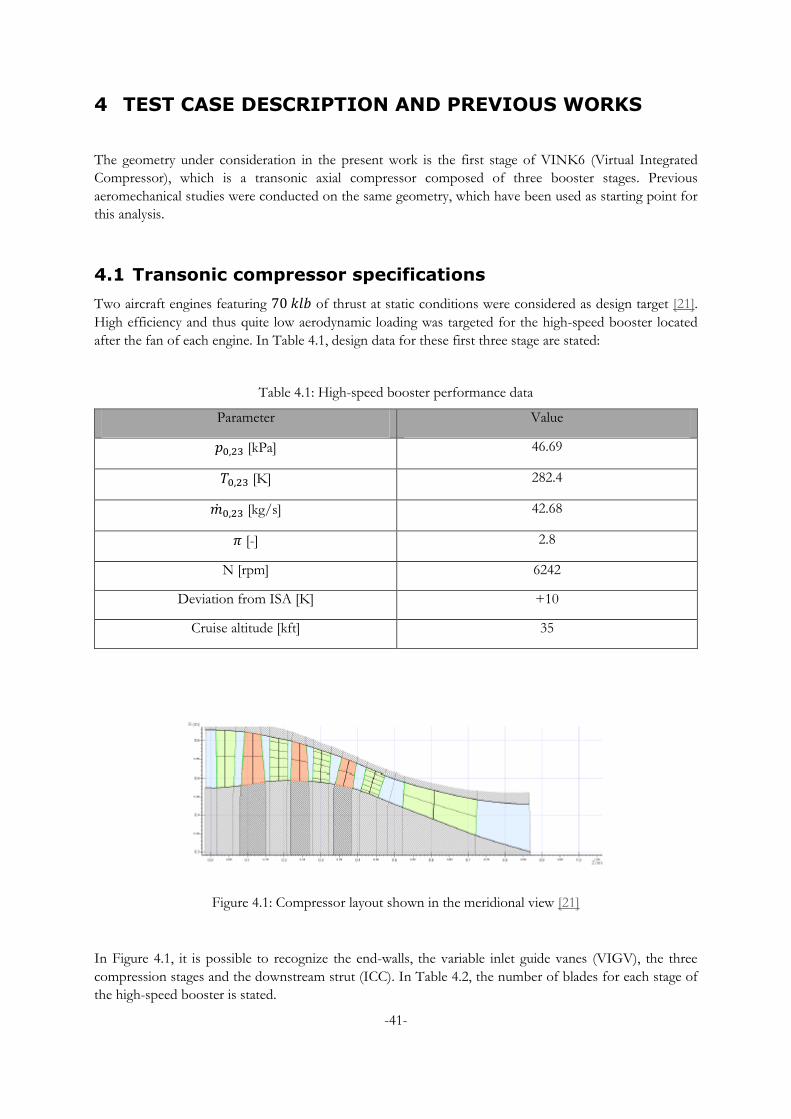
-41-
4 TEST CASE DESCRIPTION AND PREVIOUS WORKS
The geometry under consideration in the present work is the first stage of VINK6 (Virtual Integrated
Compressor), which is a transonic axial compressor composed of three booster stages. Previous
aeromechanical studies were conducted on the same geometry, which have been used as starting point for
this analysis.
4.1 Transonic compressor specifications
Two aircraft engines featuring 70 𝑘𝑙𝑏 of thrust at static conditions were considered as design target [21].
High efficiency and thus quite low aerodynamic loading was targeted for the high-speed booster located
after the fan of each engine. In Table 4.1, design data for these first three stage are stated:
Table 4.1: High-speed booster performance data
Parameter Value
𝑝0,23 [kPa] 46.69
𝑇0,23 [K] 282.4
�̇�0,23 [kg/s] 42.68
𝜋 [-] 2.8
N [rpm] 6242
Deviation from ISA [K] +10
Cruise altitude [kft] 35
Figure 4.1: Compressor layout shown in the meridional view [21]
In Figure 4.1, it is possible to recognize the end-walls, the variable inlet guide vanes (VIGV), the three
compression stages and the downstream strut (ICC). In Table 4.2, the number of blades for each stage of
the high-speed booster is stated.
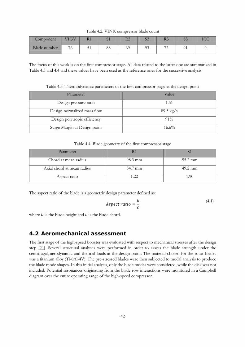
-42-
Table 4.2: VINK compressor blade count
Component VIGV R1 S1 R2 S2 R3 S3 ICC
Blade number 76 51 88 69 93 72 91 9
The focus of this work is on the first compressor stage. All data related to the latter one are summarized in
Table 4.3 and 4.4 and these values have been used as the reference ones for the successive analysis.
Table 4.3: Thermodynamic parameters of the first compressor stage at the design point
Parameter Value
Design pressure ratio 1.51
Design normalized mass flow 89.5 kg/s
Design polytropic efficiency 91%
Surge Margin at Design point 16.6%
Table 4.4: Blade geometry of the first compressor stage
Parameter R1 S1
Chord at mean radius 98.3 mm 55.2 mm
Axial chord at mean radius 54.7 mm 49.2 mm
Aspect ratio 1.22 1.90
The aspect ratio of the blade is a geometric design parameter defined as:
𝐴𝑠𝑝𝑒𝑐𝑡 𝑟𝑎𝑡𝑖𝑜 =
𝑏
𝑐
(4.1)
where 𝑏 is the blade height and 𝑐 is the blade chord.
4.2 Aeromechanical assessment
The first stage of the high-speed booster was evaluated with respect to mechanical stresses after the design
step [21]. Several structural analyses were performed in order to assess the blade strength under the
centrifugal, aerodynamic and thermal loads at the design point. The material chosen for the rotor blades
was a titanium alloy (Ti-6Al-4V). The pre-stressed blades were then subjected to modal analysis to produce
the blade mode shapes. In this initial analysis, only the blade modes were considered, while the disk was not
included. Potential resonances originating from the blade row interactions were monitored in a Campbell
diagram over the entire operating range of the high-speed compressor.
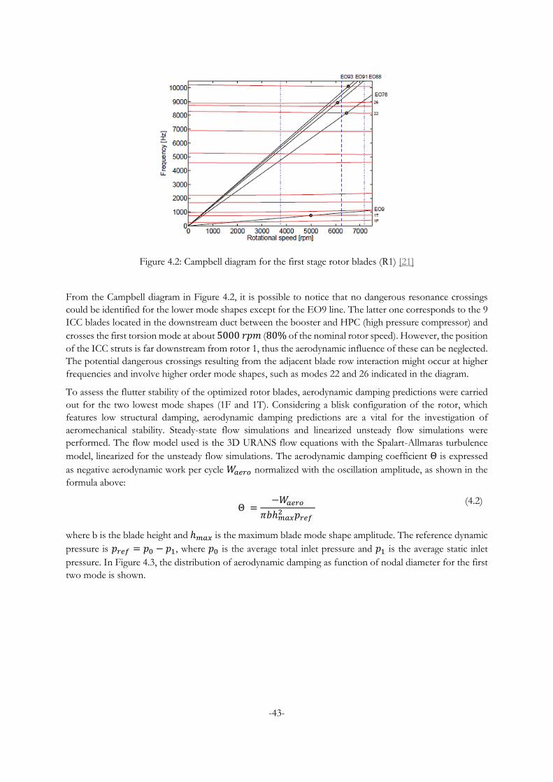
-43-
Figure 4.2: Campbell diagram for the first stage rotor blades (R1) [21]
From the Campbell diagram in Figure 4.2, it is possible to notice that no dangerous resonance crossings
could be identified for the lower mode shapes except for the EO9 line. The latter one corresponds to the 9
ICC blades located in the downstream duct between the booster and HPC (high pressure compressor) and
crosses the first torsion mode at about 5000 𝑟𝑝𝑚 (80% of the nominal rotor speed). However, the position
of the ICC struts is far downstream from rotor 1, thus the aerodynamic influence of these can be neglected.
The potential dangerous crossings resulting from the adjacent blade row interaction might occur at higher
frequencies and involve higher order mode shapes, such as modes 22 and 26 indicated in the diagram.
To assess the flutter stability of the optimized rotor blades, aerodynamic damping predictions were carried
out for the two lowest mode shapes (1F and 1T). Considering a blisk configuration of the rotor, which
features low structural damping, aerodynamic damping predictions are a vital for the investigation of
aeromechanical stability. Steady-state flow simulations and linearized unsteady flow simulations were
performed. The flow model used is the 3D URANS flow equations with the Spalart-Allmaras turbulence
model, linearized for the unsteady flow simulations. The aerodynamic damping coefficient Θ is expressed
as negative aerodynamic work per cycle 𝑊𝑎𝑒𝑟𝑜 normalized with the oscillation amplitude, as shown in the
formula above:
Θ =
−𝑊𝑎𝑒𝑟𝑜
𝜋𝑏ℎ𝑚𝑎𝑥2 𝑝𝑟𝑒𝑓
(4.2)
where b is the blade height and ℎ𝑚𝑎𝑥 is the maximum blade mode shape amplitude. The reference dynamic
pressure is 𝑝𝑟𝑒𝑓 = 𝑝0 − 𝑝1, where 𝑝0 is the average total inlet pressure and 𝑝1 is the average static inlet
pressure. In Figure 4.3, the distribution of aerodynamic damping as function of nodal diameter for the first
two mode is shown.
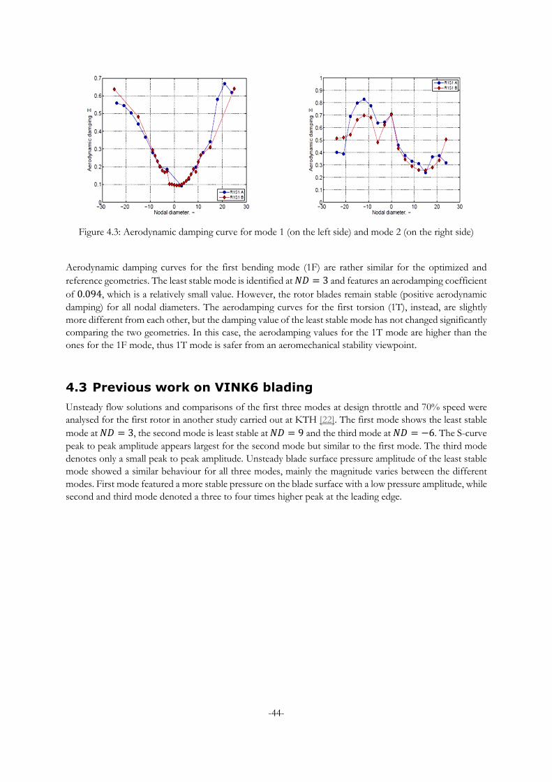
-44-
Figure 4.3: Aerodynamic damping curve for mode 1 (on the left side) and mode 2 (on the right side)
Aerodynamic damping curves for the first bending mode (1F) are rather similar for the optimized and
reference geometries. The least stable mode is identified at 𝑁𝐷 = 3 and features an aerodamping coefficient
of 0.094, which is a relatively small value. However, the rotor blades remain stable (positive aerodynamic
damping) for all nodal diameters. The aerodamping curves for the first torsion (1T), instead, are slightly
more different from each other, but the damping value of the least stable mode has not changed significantly
comparing the two geometries. In this case, the aerodamping values for the 1T mode are higher than the
ones for the 1F mode, thus 1T mode is safer from an aeromechanical stability viewpoint.
4.3 Previous work on VINK6 blading
Unsteady flow solutions and comparisons of the first three modes at design throttle and 70% speed were
analysed for the first rotor in another study carried out at KTH [22]. The first mode shows the least stable
mode at 𝑁𝐷 = 3, the second mode is least stable at 𝑁𝐷 = 9 and the third mode at 𝑁𝐷 = −6. The S-curve
peak to peak amplitude appears largest for the second mode but similar to the first mode. The third mode
denotes only a small peak to peak amplitude. Unsteady blade surface pressure amplitude of the least stable
mode showed a similar behaviour for all three modes, mainly the magnitude varies between the different
modes. First mode featured a more stable pressure on the blade surface with a low pressure amplitude, while
second and third mode denoted a three to four times higher peak at the leading edge.
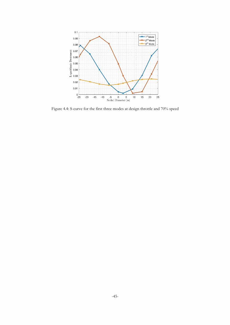
-45-
Figure 4.4: S-curve for the first three modes at design throttle and 70% speed
-46-
5 NUMERICAL METHODS
The focus of this work is on numerical techniques aiming to solve fluid flow field around compressor blades,
since the structural problem can be solved separately as previously mentioned. In turbomachinery, modeling
in frequency domain is usually used to predict the unsteady aerodynamics. The unsteady flow is in fact a
non-linear phenomenon, but switching from time domain to frequency domain, linear unsteady flow can
be assumed and this simplifies the resolution strategy. The flow can be decomposed into two parts, which
are the steady flow and an unsteady linear perturbation, which in relative terms is considered less significance
in value. Stationary flow is described by partial non-linear differential equations, while flow perturbation is
modelled with a series of partial differential equations with linear coefficients, which turn out to be
hyperbolic over time. Without losing accuracy and knowing that the unsteady flow is periodic over time,
Fourier transformation can be computed involving space-dependent complex coefficients. Each coefficient
is described by a series of partial differential equations, where time does not appear explicitly, making these
equations linearized. Essentially the equation systems obtained from this analysis require a low
computational cost without resulting in an incorrect calculation of the fluid dynamic parameters.
5.1 Computational environment
ANSYS CFX [23] is a three-dimensional finite volume method based time-implicit Navier-Stokes equation
solver. A control volume is constructed around each vertex of the mesh (structured, unstructured or hybrid)
elements and fluxes are computed at the integration points on the faces of these control volume [24]. The
discretized equations are then solved using a bounded high-resolution advection scheme similar to Barth
and Jesperson [25]. Pressure velocity coupling is carried out using the 4th order pressure smoothing Rhie
and Chow algorithm [26]. Discretized equations are then solved using the coupled algebraic multi-grid
method developed by Hutchinson and Raithby [27], and Raw [28]. Numerical effort of this method scales
linearly with the number of grid nodes in the computational domain. Steady state calculations are performed
using a pseudo-time marching approach until user defined convergence is reached. For unsteady
calculations, an iterative procedure updates the non-linear coefficients within each time step while the outer
loop advances the solution in time for time integration setup. Reynolds stresses can be computed by
different turbulence methods.
5.2 Use of RANS equations and turbulence models
Navier-Stokes equations are partial differential equations describing a flow field from a macroscopic
viewpoint. Hypothesis behind this formulation assume that the fluid is modeled as a deformable continuum
and is Newtonian (viscosity remains constant regardless fluid velocity). Using a Cartesian coordinate system,
continuity and Navier-Stokes equations can be written in the following compact form [29]:
𝑑𝑖𝑣(𝑢) = 0 (5.1a)
𝜕𝑢
𝜕𝑡+ 𝑑𝑖𝑣(𝑢𝑢) = −
1
𝜌
𝜕𝑝
𝜕𝑥+ 𝑢(𝑑𝑖𝑣𝑔𝑟𝑎𝑑(𝑢))
(5.1b)
𝜕𝑣
𝜕𝑡+ 𝑑𝑖𝑣(𝑣𝑢) = −
1
𝜌
𝜕𝑝
𝜕𝑦+ 𝑣𝑑𝑖𝑣(𝑔𝑟𝑎𝑑(𝑣))
(5.1c)
-47-
𝜕𝑤
𝜕𝑡+ 𝑑𝑖𝑣(𝑤𝑢) = −
1
𝜌
𝜕𝑝
𝜕𝑧+ 𝑣𝑑𝑖𝑣(𝑔𝑟𝑎𝑑(𝑤))
(5.1d)
In turbulent regime, equations (5.1) are not used in the above mentioned form because the computational
calculation would require an excessive cost. In fact, on industrial scale it is usually not necessary to model
exactly the turbulence phenomena, hence simplified formulation such as averaged Navier-Stokes equations
are more convenient. The latter equations describe the flow field as the sum of a stationary contribution
and a fluctuation contribution over time. For the sake of simplicity in the following related math, the fluid
is considered incompressible and features constant viscosity but the final outcomes can be extended to the
general case. Any property of the fluid 𝜓 can be written as a sum of its average value and its fluctuating part:
𝜓 = Ψ+ 𝜓′ (5.2)
where by definition the fluctuating part has time mean value that is zero. It is possible to substitute the
average and fluctuating components in equations (5.1) to obtain the following formulation:
𝑑𝑖𝑣(𝑢) = 𝑑𝑖𝑣(𝑈) (5.3a)
𝜕𝑈
𝜕𝑡+ 𝑑𝑖𝑣(𝑈𝑈) + 𝑑𝑖𝑣(𝑢′𝑢′)̅̅ ̅̅ ̅̅ ̅̅ = −
1
𝜌
𝜕𝑃
𝜕𝑥+ 𝑣𝑑𝑖𝑣(𝑔𝑟𝑎𝑑(𝑈))
(5.3b)
𝜕𝑈
𝜕𝑡+ 𝑑𝑖𝑣(𝑉𝑈) + 𝑑𝑖𝑣(𝑣′𝑢′)̅̅ ̅̅ ̅̅ ̅̅ = −
1
𝜌
𝜕𝑃
𝜕𝑦+ 𝑣𝑑𝑖𝑣(𝑔𝑟𝑎𝑑(𝑉))
(5.3c)
𝜕𝑈
𝜕𝑡+ 𝑑𝑖𝑣(𝑊𝑈) + 𝑑𝑖𝑣(𝑤′𝑢′)̅̅ ̅̅ ̅̅ ̅̅ = −
1
𝜌
𝜕𝑃
𝜕𝑧+ 𝑣𝑑𝑖𝑣(𝑔𝑟𝑎𝑑(𝑊))
(5.3d)
By comparing equations (5.3) and (5.1), except for the mass conservation, a new term appears in each new
equation. These additional contributions, which are the product of two fluctuating velocities, derive from
turbulent vortices and are called Reynolds stresses. These stresses are null only if the two components of
fluctuating velocity are both random and independent of each other. In most cases, this never happens and,
on the other hand, these terms are very high compared to purely viscous stress. Equations (5.3) are referred
to as RANS equations. If the average fluctuation in time does not exceed 5%, then the density variation is
not important up to Mach number equal to 3 or 5. If the threshold value is exceeded, starting from Mach
number equal to 1 there are important variations in density and after integrating average and fluctuating
terms in time (Favre averaging), RANS equations for a compressible fluid are obtained:
𝜕�̅�
𝜕𝑡+ 𝑑𝑖𝑣(�̅��̃�) = 0
(5.4a)
𝜕�̅��̃�
𝜕𝑡+ 𝑑𝑖𝑣(�̅��̃��̃�) = −
𝜕�̅�
𝜕𝑥+ 𝑑𝑖𝑣 (𝜇𝑔𝑟𝑎𝑑(�̃�)) +
+ [−𝜕�̅�𝑢′2̅̅ ̅̅ ̅̅
𝜕𝑥−𝜕�̅�𝑢′𝑣′̅̅ ̅̅ ̅̅ ̅
𝜕𝑦−𝜕�̅�𝑢′𝑤′̅̅ ̅̅ ̅̅ ̅̅
𝜕𝑧] + 𝑆𝑀𝑥
(5.4b)
𝜕�̅��̃�
𝜕𝑡+ 𝑑𝑖𝑣(�̅��̃��̃�) = −
𝜕�̅�
𝜕𝑦+ 𝑑𝑖𝑣 (𝜇𝑔𝑟𝑎𝑑(�̃�)) +
+ [−𝜕�̅�𝑢′𝑣′̅̅ ̅̅ ̅̅ ̅
𝜕𝑥−𝜕�̅�𝑣′2̅̅ ̅̅ ̅̅
𝜕𝑦−𝜕�̅�𝑢′𝑤′̅̅ ̅̅ ̅̅ ̅̅
𝜕𝑧] + 𝑆𝑀𝑦
(5.4c)
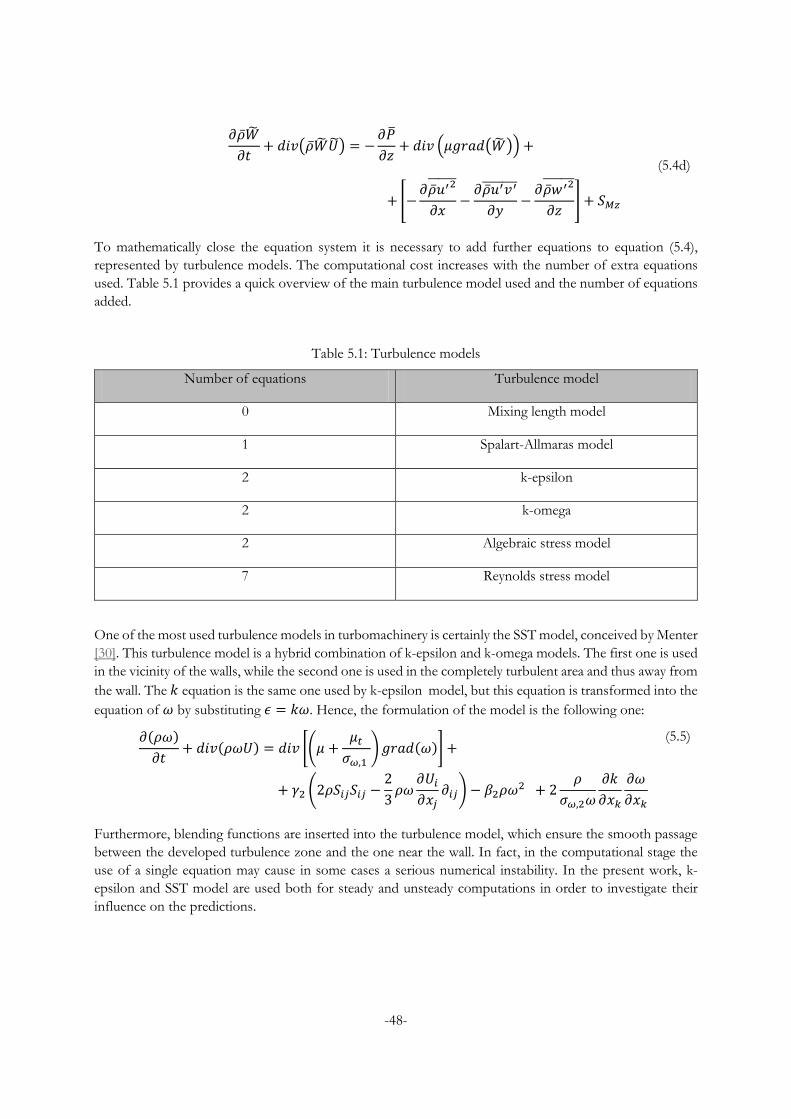
-48-
𝜕�̅��̃�
𝜕𝑡+ 𝑑𝑖𝑣(�̅��̃��̃�) = −
𝜕�̅�
𝜕𝑧+ 𝑑𝑖𝑣 (𝜇𝑔𝑟𝑎𝑑(�̃�)) +
+ [−𝜕�̅�𝑢′2̅̅ ̅̅ ̅̅
𝜕𝑥−𝜕�̅�𝑢′𝑣′̅̅ ̅̅ ̅̅ ̅
𝜕𝑦−𝜕�̅�𝑤′2̅̅ ̅̅ ̅̅ ̅
𝜕𝑧] + 𝑆𝑀𝑧
(5.4d)
To mathematically close the equation system it is necessary to add further equations to equation (5.4),
represented by turbulence models. The computational cost increases with the number of extra equations
used. Table 5.1 provides a quick overview of the main turbulence model used and the number of equations
added.
Table 5.1: Turbulence models
Number of equations Turbulence model
0 Mixing length model
1 Spalart-Allmaras model
2 k-epsilon
2 k-omega
2 Algebraic stress model
7 Reynolds stress model
One of the most used turbulence models in turbomachinery is certainly the SST model, conceived by Menter
[30]. This turbulence model is a hybrid combination of k-epsilon and k-omega models. The first one is used
in the vicinity of the walls, while the second one is used in the completely turbulent area and thus away from
the wall. The 𝑘 equation is the same one used by k-epsilon model, but this equation is transformed into the
equation of 𝜔 by substituting 𝜖 = 𝑘𝜔. Hence, the formulation of the model is the following one:
𝜕(𝜌𝜔)
𝜕𝑡+ 𝑑𝑖𝑣(𝜌𝜔𝑈) = 𝑑𝑖𝑣 [(𝜇 +
𝜇𝑡𝜎𝜔,1
) 𝑔𝑟𝑎𝑑(𝜔)] +
+ 𝛾2 (2𝜌𝑆𝑖𝑗𝑆𝑖𝑗 −2
3𝜌𝜔
𝜕𝑈𝑖𝜕𝑥𝑗
𝜕𝑖𝑗) − 𝛽2𝜌𝜔2 + 2
𝜌
𝜎𝜔,2𝜔
𝜕𝑘
𝜕𝑥𝑘
𝜕𝜔
𝜕𝑥𝑘
(5.5)
Furthermore, blending functions are inserted into the turbulence model, which ensure the smooth passage
between the developed turbulence zone and the one near the wall. In fact, in the computational stage the
use of a single equation may cause in some cases a serious numerical instability. In the present work, k-
epsilon and SST model are used both for steady and unsteady computations in order to investigate their
influence on the predictions.
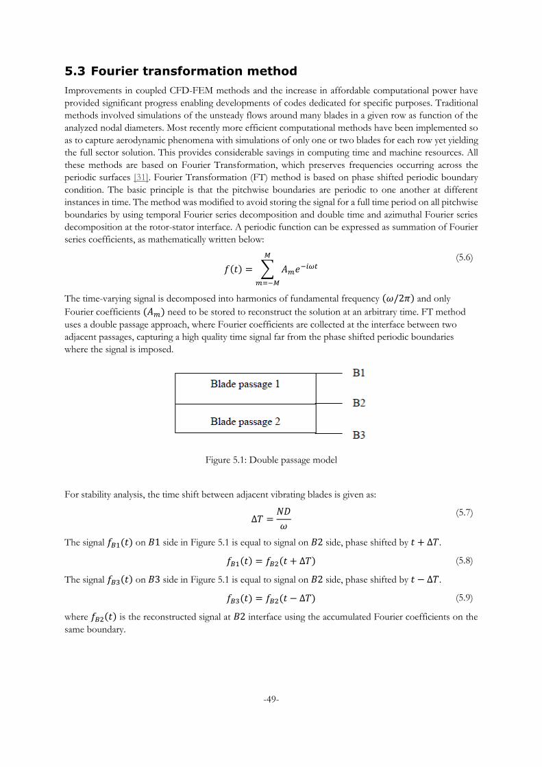
-49-
5.3 Fourier transformation method
Improvements in coupled CFD-FEM methods and the increase in affordable computational power have
provided significant progress enabling developments of codes dedicated for specific purposes. Traditional
methods involved simulations of the unsteady flows around many blades in a given row as function of the
analyzed nodal diameters. Most recently more efficient computational methods have been implemented so
as to capture aerodynamic phenomena with simulations of only one or two blades for each row yet yielding
the full sector solution. This provides considerable savings in computing time and machine resources. All
these methods are based on Fourier Transformation, which preserves frequencies occurring across the
periodic surfaces [31]. Fourier Transformation (FT) method is based on phase shifted periodic boundary
condition. The basic principle is that the pitchwise boundaries are periodic to one another at different
instances in time. The method was modified to avoid storing the signal for a full time period on all pitchwise
boundaries by using temporal Fourier series decomposition and double time and azimuthal Fourier series
decomposition at the rotor-stator interface. A periodic function can be expressed as summation of Fourier
series coefficients, as mathematically written below:
𝑓(𝑡) = ∑ 𝐴𝑚𝑒−𝑖𝜔𝑡
𝑀
𝑚=−𝑀
(5.6)
The time-varying signal is decomposed into harmonics of fundamental frequency (𝜔/2𝜋) and only
Fourier coefficients (𝐴𝑚) need to be stored to reconstruct the solution at an arbitrary time. FT method
uses a double passage approach, where Fourier coefficients are collected at the interface between two
adjacent passages, capturing a high quality time signal far from the phase shifted periodic boundaries
where the signal is imposed.
Figure 5.1: Double passage model
For stability analysis, the time shift between adjacent vibrating blades is given as:
∆𝑇 =
𝑁𝐷
𝜔
(5.7)
The signal 𝑓𝐵1(𝑡) on 𝐵1 side in Figure 5.1 is equal to signal on 𝐵2 side, phase shifted by 𝑡 + ∆𝑇.
𝑓𝐵1(𝑡) = 𝑓𝐵2(𝑡 + ∆𝑇) (5.8)
The signal 𝑓𝐵3(𝑡) on 𝐵3 side in Figure 5.1 is equal to signal on 𝐵2 side, phase shifted by 𝑡 − ∆𝑇.
𝑓𝐵3(𝑡) = 𝑓𝐵2(𝑡 − ∆𝑇) (5.9)
where 𝑓𝐵2(𝑡) is the reconstructed signal at 𝐵2 interface using the accumulated Fourier coefficients on the
same boundary.
-50-
5.4 Harmonic balance analysis
When the unsteady motion assumes a greater importance, then solutions obtained by the linearized
equations may not be representative of the investigated flow field. Therefore, in that case it might be
necessary to apply a different numerical approach, such as the harmonic balance method, which is able to
model harsh conditions of shock waves and sharp separation of the boundary layer, to get better numerical
predictions. For the sake of simplicity in the following related math, the fluid is considered two-dimensional,
non-viscous, non-conductive and with constant specific heat. The flow can be then modeled through two-
dimensional Euler's equations [32]:
𝜕𝑈
𝜕𝑡+𝜕𝐹(𝑈)
𝜕𝑥+𝜕𝐺(𝑈)
𝜕𝑦= 0
(5.10)
Conservation variables and flux terms present in equation (5.10) can be expressed as follows:
𝑈 = [
𝜌𝜌𝑢𝜌𝑣𝑝𝑒
] 𝐹 = [
𝜌𝑢
𝜌𝑢2 + 𝑝𝜌𝑢𝑣𝜌𝑢ℎ
] 𝐺 = [
𝜌𝑣𝜌𝑢𝑣
𝜌𝑣2 + 𝑝𝜌𝑣ℎ
]
(5.11)
In equations (5.11) velocity, density, pressure and total enthalpy terms appear. By considering the flow
temporally periodic, equation (5.12) can be written:
𝑈(𝑥, 𝑦, 𝑡) = 𝑈(𝑥, 𝑦, 𝑡 + 𝑇) (5.12)
where 𝑇 represents the period of the unsteadiness. Space periodicity requires that the following condition
is met:
𝑈(𝑥, 𝑦 + 𝐺, 𝑡) = 𝑈(𝑥, 𝑦, 𝑡 + ∆𝑇) (5.13)
where 𝐺 is the blade pitch and ∆𝑇 is time interval related to 𝐼𝐵𝑃𝐴. For a given frequency and given 𝐼𝐵𝑃𝐴,
the period is defined as 𝑇 = 2𝜋/𝜔 and thus the time interval related to 𝐼𝐵𝑃𝐴 is defined as ∆𝑇 = 𝐼𝐵𝑃𝐴/𝜔.
Since the flow is periodic in time and in space, then the variables can be written in Fourier series, where the
coefficients are space-dependent functions.
𝜌(𝑥, 𝑦, 𝑡) =∑𝑅𝑛(𝑥, 𝑦)𝑒
𝑖𝜔𝑛𝑡
𝑛
(5.14a)
𝜌𝑢(𝑥, 𝑦, 𝑡) =∑𝑈𝑛(𝑥, 𝑦)𝑒
𝑖𝜔𝑛𝑡
𝑛
(5.14b)
𝜌𝑣(𝑥, 𝑦, 𝑡) =∑𝑉𝑛(𝑥, 𝑦)𝑒
𝑖𝜔𝑛𝑡
𝑛
(5.14c)
𝜌𝑒(𝑥, 𝑦, 𝑡) =∑𝐸𝑛(𝑥, 𝑦)𝑒
𝑖𝜔𝑛𝑡
𝑛
(5.14d)
In equations (5.14) summations are truncated to a finite number of terms ranging between ±𝑁. In the
definition of enthalpy and pressure, implicitly used in equation (5.10), the density can appear at the
denominator of each term. Expressing the latter one in Fourier series, it is possible to obtain:
1
𝜌(𝑥, 𝑦, 𝑡)=∑Γ𝑛(𝑥, 𝑦)𝑒
𝑖𝜔𝑛𝑡
𝑛
(5.15)
-51-
If equation (5.14a) is combined with equation (5.15), the following result is obtained:
𝜌 ∙1
𝜌= [∑𝑅𝑛(𝑥, 𝑦)𝑒
𝑖𝜔𝑛𝑡
𝑛
]⨂ [∑Γ𝑛(𝑥, 𝑦)𝑒𝑖𝜔𝑛𝑡
𝑚
] = 1 (5.16)
To satisfy equation(5.16) it is necessary, except for the null-frequency terms (𝑛 +𝑚 = 0), that the series
coefficients are null. For example, if the force is modeled with N = 2 harmonics, one can get the following
system to solve:
[ 𝑅0 𝑅−1 𝑅−2 0 0𝑅1 𝑅0 𝑅−1 𝑅−2 0𝑅2 𝑅1 𝑅0 𝑅−1 𝑅−20 𝑅2 𝑅1 𝑅0 𝑅−10 0 𝑅2 𝑅1 𝑅0 ]
[ Γ−2Γ−1Γ0Γ1Γ2 ]
=
[ 00100]
(5.17)
The system obtained in matrix equation (5.17) must also be obtained for mass, energy and momentum
conservation equations. Basically, for each written equation, terms can be grouped for frequency order and
each group can be placed in an equation equal to zero. It is possible to group all the equations formulated,
using the following vector notation:
𝜕�̃�(�̃�)
𝜕𝑥+𝜕�̃�(�̃�)
𝜕𝑦+ �̃�(�̃�) = 0
(5.18)
where in equation (5.18) vectors �̃� and �̃� can be written again as:
�̃� =
[ 𝑅0𝑈0𝑉0𝐸0𝑅1𝑈1𝑉1𝐸1… ]
�̃� = 𝑖𝜔
[ 𝑅0𝑈0𝑉0𝐸0𝑅1𝑈1𝑉1𝐸1… ]
(5.19)
while �̃� and �̃�, more complicated to write, can however be defined as non-linear functions of the Fourier
series coefficients for the conservation variables �̃�. Since �̃� is composed by real quantities, then the
conjugate complex of the 𝑈𝑁 must be equal to the quantity 𝑈−𝑁. The problem is now simplified because
Fourier harmonic terms vary only for 𝑁 > 0. If we assume that the sufficient number of harmonics to
describe the problem is 𝑁, then for each variable we must store 𝑁 coefficients for the real part, 𝑁
coefficients for the complex part and one for the constant term. In total 2𝑁 + 1 terms for each variable
have to be calculated. Thus, the computational cost of this method requires the resolution of 𝑁3 operations,
so the algorithm can be very heavily weighted by increasing the number of harmonics describing the
problem. Moreover, for viscous flows, the equations of turbulence are not quickly modeled in the algebraic
form and this creates considerable inconveniences. To avoid this number of problems, one could think of
constructing �̃�, �̃� and �̃� by evaluating the temporal behavior of 𝑈, 𝐹 and 𝐺 in the equally spaced points
over a period of time. In practice (5.20) can be written:
�̃� = 𝐸𝑈∗ (5.20)
where 𝑈∗ is the vector of conservation variables in the 2𝑁 + 1 equally spaced points, while 𝐸 is the discrete
matrix of Fourier transformation. Replacing equation (5.20) within equation (5.18), the following expression
is obtained:
-52-
𝜕𝐸𝐹∗
𝜕𝑥+𝜕𝐸𝐺∗
𝜕𝑦+ 𝑖𝜔𝑁𝐸𝑈∗ = 0
(5.21)
where in equation (5.21) 𝑁 is a diagonal matrix in which every 𝑁 entry corresponds to the 𝑁 harmonic. By
pre-multiplying equation (5.21) for the inverse of the matrix 𝐸, the third term assumes the following form:
𝑖𝜔𝐸−1𝑁𝐸𝑈∗ = 𝑆∗ ≈
𝜕𝑈∗
𝜕𝑡
(5.22)
In this way the spectral operator coming before the term 𝑈∗ can be approximated with the operator 𝜕/𝜕𝑡. The final expression of Euler's equations, using the harmonic equilibrium method, is reduced to:
𝜕𝐹∗
𝜕𝑥+𝜕𝐺∗
𝜕𝑦+ 𝑆∗ = 0
(5.23)
Using the discrete matrix of the Fourier transformation, the flow can be resolved more easily. Moreover,
the method can be used not only to solve the Euler equations, but also to find a solution for Navier-Stokes
equations that was not allowed by equation (5.18). A pseudo-temporal term must be introduced in order to
solve the problem with the aid of conventional CFD techniques. Basically, equation (5.23) turns into (5.24):
𝜕𝑈∗
𝜕𝜏+𝜕𝐹∗
𝜕𝑥+𝜕𝐺∗
𝜕𝑦+ 𝑆∗ = 0
(5.24)
where the term 𝜏 is seen as a dummy temporal variable. Now it is possible to use the classic method of
"time-marching" to obtain a stationary solution, thus canceling the dummy term. Note that the pseudo-
temporal harmonic equilibrium equation is very similar to Euler equation (5.10), with the difference that to
calculate the value of 𝑆∗ the spectral operator is used. In this way the number of operations is reduced to
the order 𝑁2 and for the computation of the flux vector only N operations are required.
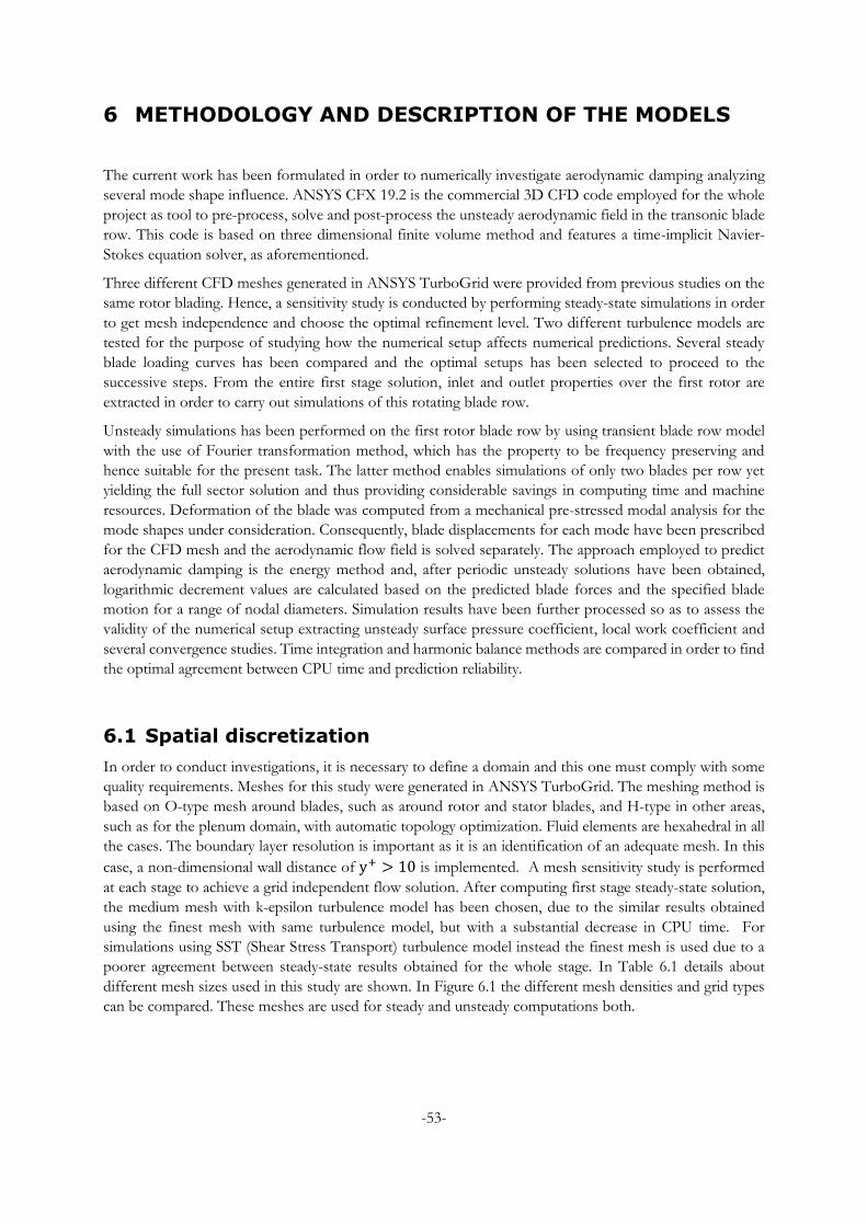
-53-
6 METHODOLOGY AND DESCRIPTION OF THE MODELS
The current work has been formulated in order to numerically investigate aerodynamic damping analyzing
several mode shape influence. ANSYS CFX 19.2 is the commercial 3D CFD code employed for the whole
project as tool to pre-process, solve and post-process the unsteady aerodynamic field in the transonic blade
row. This code is based on three dimensional finite volume method and features a time-implicit Navier-
Stokes equation solver, as aforementioned.
Three different CFD meshes generated in ANSYS TurboGrid were provided from previous studies on the
same rotor blading. Hence, a sensitivity study is conducted by performing steady-state simulations in order
to get mesh independence and choose the optimal refinement level. Two different turbulence models are
tested for the purpose of studying how the numerical setup affects numerical predictions. Several steady
blade loading curves has been compared and the optimal setups has been selected to proceed to the
successive steps. From the entire first stage solution, inlet and outlet properties over the first rotor are
extracted in order to carry out simulations of this rotating blade row.
Unsteady simulations has been performed on the first rotor blade row by using transient blade row model
with the use of Fourier transformation method, which has the property to be frequency preserving and
hence suitable for the present task. The latter method enables simulations of only two blades per row yet
yielding the full sector solution and thus providing considerable savings in computing time and machine
resources. Deformation of the blade was computed from a mechanical pre-stressed modal analysis for the
mode shapes under consideration. Consequently, blade displacements for each mode have been prescribed
for the CFD mesh and the aerodynamic flow field is solved separately. The approach employed to predict
aerodynamic damping is the energy method and, after periodic unsteady solutions have been obtained,
logarithmic decrement values are calculated based on the predicted blade forces and the specified blade
motion for a range of nodal diameters. Simulation results have been further processed so as to assess the
validity of the numerical setup extracting unsteady surface pressure coefficient, local work coefficient and
several convergence studies. Time integration and harmonic balance methods are compared in order to find
the optimal agreement between CPU time and prediction reliability.
6.1 Spatial discretization
In order to conduct investigations, it is necessary to define a domain and this one must comply with some
quality requirements. Meshes for this study were generated in ANSYS TurboGrid. The meshing method is
based on O-type mesh around blades, such as around rotor and stator blades, and H-type in other areas,
such as for the plenum domain, with automatic topology optimization. Fluid elements are hexahedral in all
the cases. The boundary layer resolution is important as it is an identification of an adequate mesh. In this
case, a non-dimensional wall distance of y+ > 10 is implemented. A mesh sensitivity study is performed
at each stage to achieve a grid independent flow solution. After computing first stage steady-state solution,
the medium mesh with k-epsilon turbulence model has been chosen, due to the similar results obtained
using the finest mesh with same turbulence model, but with a substantial decrease in CPU time. For
simulations using SST (Shear Stress Transport) turbulence model instead the finest mesh is used due to a
poorer agreement between steady-state results obtained for the whole stage. In Table 6.1 details about
different mesh sizes used in this study are shown. In Figure 6.1 the different mesh densities and grid types
can be compared. These meshes are used for steady and unsteady computations both.
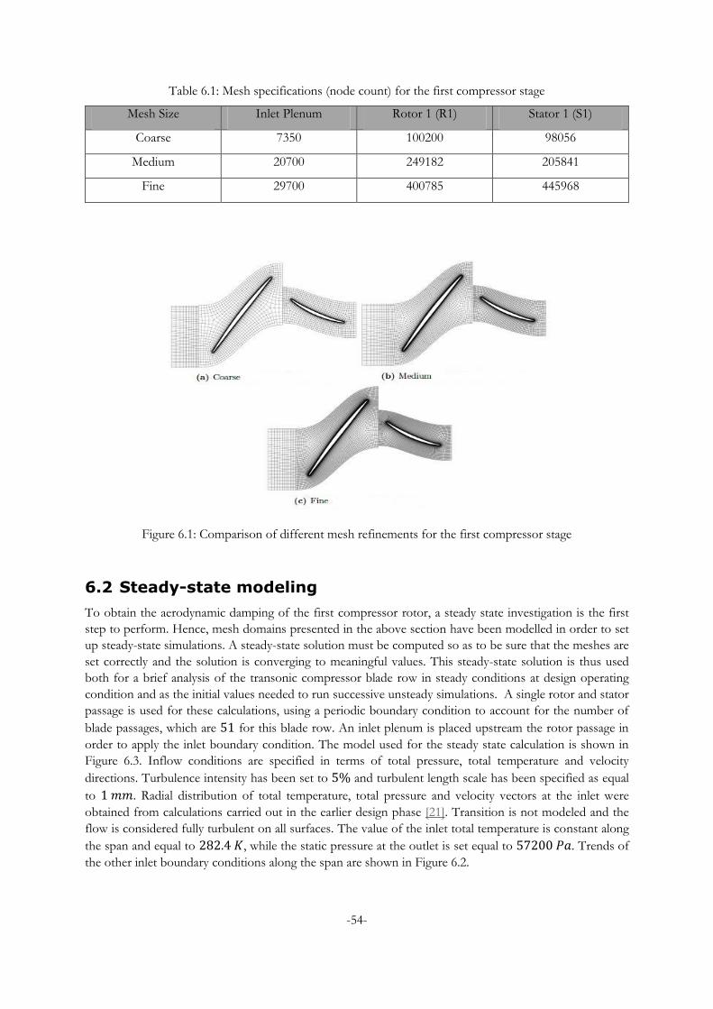
-54-
Table 6.1: Mesh specifications (node count) for the first compressor stage
Mesh Size Inlet Plenum Rotor 1 (R1) Stator 1 (S1)
Coarse 7350 100200 98056
Medium 20700 249182 205841
Fine 29700 400785 445968
Figure 6.1: Comparison of different mesh refinements for the first compressor stage
6.2 Steady-state modeling
To obtain the aerodynamic damping of the first compressor rotor, a steady state investigation is the first
step to perform. Hence, mesh domains presented in the above section have been modelled in order to set
up steady-state simulations. A steady-state solution must be computed so as to be sure that the meshes are
set correctly and the solution is converging to meaningful values. This steady-state solution is thus used
both for a brief analysis of the transonic compressor blade row in steady conditions at design operating
condition and as the initial values needed to run successive unsteady simulations. A single rotor and stator
passage is used for these calculations, using a periodic boundary condition to account for the number of
blade passages, which are 51 for this blade row. An inlet plenum is placed upstream the rotor passage in
order to apply the inlet boundary condition. The model used for the steady state calculation is shown in
Figure 6.3. Inflow conditions are specified in terms of total pressure, total temperature and velocity
directions. Turbulence intensity has been set to 5% and turbulent length scale has been specified as equal
to 1 𝑚𝑚. Radial distribution of total temperature, total pressure and velocity vectors at the inlet were
obtained from calculations carried out in the earlier design phase [21]. Transition is not modeled and the
flow is considered fully turbulent on all surfaces. The value of the inlet total temperature is constant along
the span and equal to 282.4 𝐾, while the static pressure at the outlet is set equal to 57200 𝑃𝑎. Trends of
the other inlet boundary conditions along the span are shown in Figure 6.2.
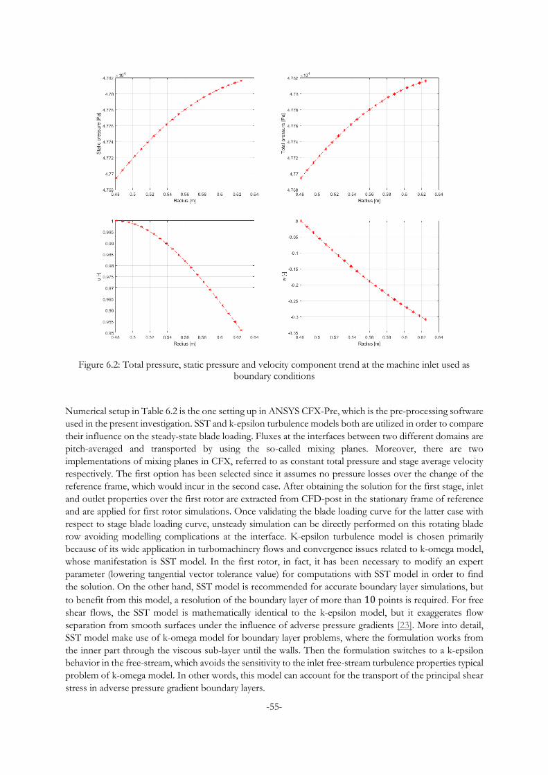
-55-
Figure 6.2: Total pressure, static pressure and velocity component trend at the machine inlet used as boundary conditions
Numerical setup in Table 6.2 is the one setting up in ANSYS CFX-Pre, which is the pre-processing software
used in the present investigation. SST and k-epsilon turbulence models both are utilized in order to compare
their influence on the steady-state blade loading. Fluxes at the interfaces between two different domains are
pitch-averaged and transported by using the so-called mixing planes. Moreover, there are two
implementations of mixing planes in CFX, referred to as constant total pressure and stage average velocity
respectively. The first option has been selected since it assumes no pressure losses over the change of the
reference frame, which would incur in the second case. After obtaining the solution for the first stage, inlet
and outlet properties over the first rotor are extracted from CFD-post in the stationary frame of reference
and are applied for first rotor simulations. Once validating the blade loading curve for the latter case with
respect to stage blade loading curve, unsteady simulation can be directly performed on this rotating blade
row avoiding modelling complications at the interface. K-epsilon turbulence model is chosen primarily
because of its wide application in turbomachinery flows and convergence issues related to k-omega model,
whose manifestation is SST model. In the first rotor, in fact, it has been necessary to modify an expert
parameter (lowering tangential vector tolerance value) for computations with SST model in order to find
the solution. On the other hand, SST model is recommended for accurate boundary layer simulations, but
to benefit from this model, a resolution of the boundary layer of more than 10 points is required. For free
shear flows, the SST model is mathematically identical to the k-epsilon model, but it exaggerates flow
separation from smooth surfaces under the influence of adverse pressure gradients [23]. More into detail,
SST model make use of k-omega model for boundary layer problems, where the formulation works from
the inner part through the viscous sub-layer until the walls. Then the formulation switches to a k-epsilon
behavior in the free-stream, which avoids the sensitivity to the inlet free-stream turbulence properties typical
problem of k-omega model. In other words, this model can account for the transport of the principal shear
stress in adverse pressure gradient boundary layers.
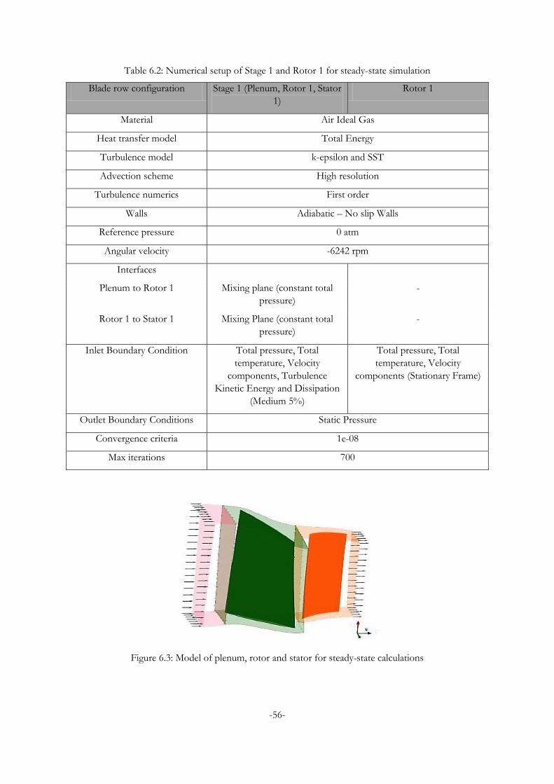
-56-
Table 6.2: Numerical setup of Stage 1 and Rotor 1 for steady-state simulation
Blade row configuration Stage 1 (Plenum, Rotor 1, Stator
1)
Rotor 1
Material Air Ideal Gas
Heat transfer model Total Energy
Turbulence model k-epsilon and SST
Advection scheme High resolution
Turbulence numerics First order
Walls Adiabatic – No slip Walls
Reference pressure 0 atm
Angular velocity -6242 rpm
Interfaces
Plenum to Rotor 1 Mixing plane (constant total
pressure)
-
Rotor 1 to Stator 1 Mixing Plane (constant total
pressure)
-
Inlet Boundary Condition Total pressure, Total
temperature, Velocity
components, Turbulence
Kinetic Energy and Dissipation
(Medium 5%)
Total pressure, Total
temperature, Velocity
components (Stationary Frame)
Outlet Boundary Conditions Static Pressure
Convergence criteria 1e-08
Max iterations 700
Figure 6.3: Model of plenum, rotor and stator for steady-state calculations
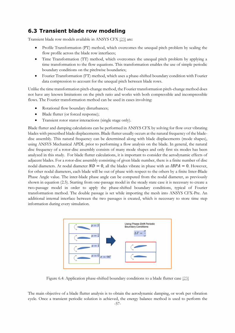
-57-
6.3 Transient blade row modeling
Transient blade row models available in ANSYS CFX [23] are:
Profile Transformation (PT) method, which overcomes the unequal pitch problem by scaling the
flow profile across the blade row interfaces;
Time Transformation (TT) method, which overcomes the unequal pitch problem by applying a
time transformation to the flow equations. This transformation enables the use of simple periodic
boundary conditions on the pitchwise boundaries;
Fourier Transformation (FT) method, which uses a phase-shifted boundary condition with Fourier
data compression to account for the unequal pitch between blade rows.
Unlike the time transformation pitch-change method, the Fourier transformation pitch-change method does
not have any known limitations on the pitch ratio and works with both compressible and incompressible
flows. The Fourier transformation method can be used in cases involving:
Rotational flow boundary disturbances;
Blade flutter (or forced response);
Transient rotor stator interactions (single stage only).
Blade flutter and damping calculations can be performed in ANSYS CFX by solving for flow over vibrating
blades with prescribed blade displacements. Blade flutter usually occurs at the natural frequency of the blade-
disc assembly. This natural frequency can be determined along with blade displacements (mode shapes),
using ANSYS Mechanical APDL prior to performing a flow analysis on the blade. In general, the natural
disc frequency of a rotor-disc assembly consists of many mode shapes and only first six modes has been
analyzed in this study. For blade flutter calculations, it is important to consider the aerodynamic effects of
adjacent blades. For a rotor-disc assembly consisting of given blade number, there is a finite number of disc
nodal diameters. At nodal diameter 𝑁𝐷 = 0, all the blades vibrate in phase with an 𝐼𝐵𝑃𝐴 = 0. However,
for other nodal diameters, each blade will be out of phase with respect to the others by a finite Inter-Blade
Phase Angle value. The inter-blade phase angle can be computed from the nodal diameter, as previously
shown in equation (2.5). Starting from one-passage model in the steady state case it is necessary to create a
two-passage model in order to apply the phase-shifted boundary conditions, typical of Fourier
transformation method. The double passage is set while importing the mesh into ANSYS CFX-Pre. An
additional internal interface between the two passages is created, which is necessary to store time step
information during every simulation.
Figure 6.4: Application phase-shifted boundary conditions to a blade flutter case [23]
The main objective of a blade flutter analysis is to obtain the aerodynamic damping, or work per vibration
cycle. Once a transient periodic solution is achieved, the energy balance method is used to perform the
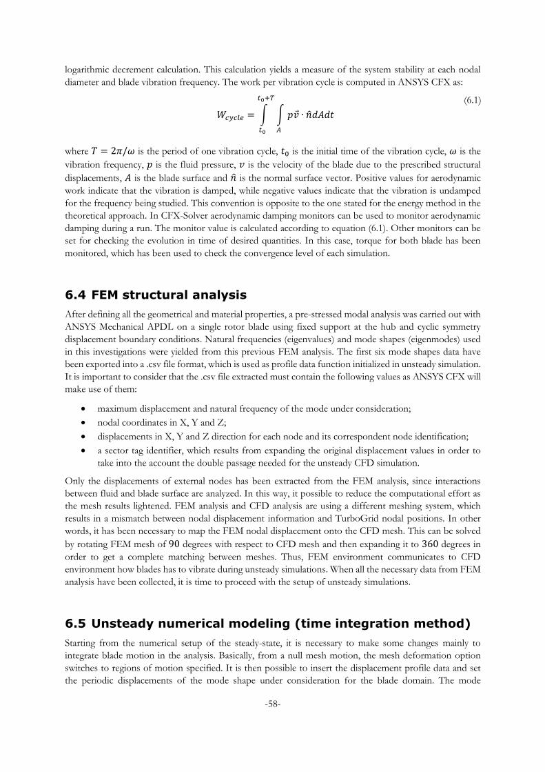
-58-
logarithmic decrement calculation. This calculation yields a measure of the system stability at each nodal
diameter and blade vibration frequency. The work per vibration cycle is computed in ANSYS CFX as:
𝑊𝑐𝑦𝑐𝑙𝑒 = ∫ ∫ 𝑝�⃗� ∙ �̂�𝑑𝐴𝑑𝑡
𝐴
𝑡0+𝑇
𝑡0
(6.1)
where 𝑇 = 2𝜋/𝜔 is the period of one vibration cycle, 𝑡0 is the initial time of the vibration cycle, 𝜔 is the
vibration frequency, 𝑝 is the fluid pressure, 𝑣 is the velocity of the blade due to the prescribed structural
displacements, 𝐴 is the blade surface and �̂� is the normal surface vector. Positive values for aerodynamic
work indicate that the vibration is damped, while negative values indicate that the vibration is undamped
for the frequency being studied. This convention is opposite to the one stated for the energy method in the
theoretical approach. In CFX-Solver aerodynamic damping monitors can be used to monitor aerodynamic
damping during a run. The monitor value is calculated according to equation (6.1). Other monitors can be
set for checking the evolution in time of desired quantities. In this case, torque for both blade has been
monitored, which has been used to check the convergence level of each simulation.
6.4 FEM structural analysis
After defining all the geometrical and material properties, a pre-stressed modal analysis was carried out with
ANSYS Mechanical APDL on a single rotor blade using fixed support at the hub and cyclic symmetry
displacement boundary conditions. Natural frequencies (eigenvalues) and mode shapes (eigenmodes) used
in this investigations were yielded from this previous FEM analysis. The first six mode shapes data have
been exported into a .csv file format, which is used as profile data function initialized in unsteady simulation.
It is important to consider that the .csv file extracted must contain the following values as ANSYS CFX will
make use of them:
maximum displacement and natural frequency of the mode under consideration;
nodal coordinates in X, Y and Z;
displacements in X, Y and Z direction for each node and its correspondent node identification;
a sector tag identifier, which results from expanding the original displacement values in order to
take into the account the double passage needed for the unsteady CFD simulation.
Only the displacements of external nodes has been extracted from the FEM analysis, since interactions
between fluid and blade surface are analyzed. In this way, it possible to reduce the computational effort as
the mesh results lightened. FEM analysis and CFD analysis are using a different meshing system, which
results in a mismatch between nodal displacement information and TurboGrid nodal positions. In other
words, it has been necessary to map the FEM nodal displacement onto the CFD mesh. This can be solved
by rotating FEM mesh of 90 degrees with respect to CFD mesh and then expanding it to 360 degrees in
order to get a complete matching between meshes. Thus, FEM environment communicates to CFD
environment how blades has to vibrate during unsteady simulations. When all the necessary data from FEM
analysis have been collected, it is time to proceed with the setup of unsteady simulations.
6.5 Unsteady numerical modeling (time integration method)
Starting from the numerical setup of the steady-state, it is necessary to make some changes mainly to
integrate blade motion in the analysis. Basically, from a null mesh motion, the mesh deformation option
switches to regions of motion specified. It is then possible to insert the displacement profile data and set
the periodic displacements of the mode shape under consideration for the blade domain. The mode
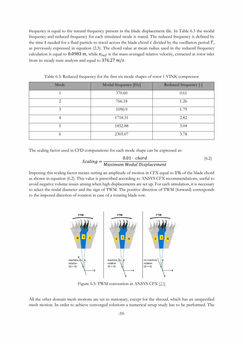
-59-
frequency is equal to the natural frequency present in the blade displacement file. In Table 6.3 the modal
frequency and reduced frequency for each simulated mode is stated. The reduced frequency is defined by
the time 𝑡 needed for a fluid particle to travel across the blade chord 𝑐 divided by the oscillation period 𝑇,
as previously expressed in equation (2.3). The chord value at mean radius used in the reduced frequency
calculation is equal to 0.0983 𝑚, while 𝑣𝑟𝑒𝑓 is the mass-averaged relative velocity, extracted at rotor inlet
from its steady state analysis and equal to 376.27 𝑚/𝑠.
Table 6.3: Reduced frequency for the first six mode shapes of rotor 1 VINK compressor
Mode Modal frequency [Hz] Reduced frequency [-]
1 370.60 0.61
2 766.18 1.26
3 1090.9 1.79
4 1718.31 2.82
5 1852.88 3.04
6 2305.07 3.78
The scaling factor used in CFD computations for each mode shape can be expressed as:
𝑆𝑐𝑎𝑙𝑖𝑛𝑔 =
0.01 ∙ 𝑐ℎ𝑜𝑟𝑑
𝑀𝑎𝑥𝑖𝑚𝑢𝑚 𝑀𝑜𝑑𝑎𝑙 𝐷𝑖𝑠𝑝𝑙𝑎𝑐𝑒𝑚𝑒𝑛𝑡
(6.2)
Imposing this scaling factor means setting an amplitude of motion in CFX equal to 1% of the blade chord
as shown in equation (6.2). This value is prescribed according to ANSYS CFX recommendations, useful to
avoid negative volume issues arising when high displacements are set up. For each simulation, it is necessary
to select the nodal diameter and the sign of TWM. The positive direction of TWM (forward) corresponds
to the imposed direction of rotation in case of a rotating blade row.
Figure 6.5: TWM convention in ANSYS CFX [23]
All the other domain mesh motions are set to stationary, except for the shroud, which has an unspecified
mesh motion. In order to achieve converged solutions a numerical setup study has to be performed. The
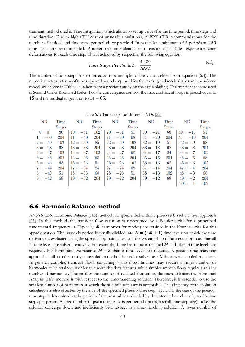
-60-
transient method used is Time Integration, which allows to set up values for the time period, time steps and
time duration. Due to high CPU cost of unsteady simulations, ANSYS CFX recommendations for the
number of periods and time steps per period are practiced. In particular a minimum of 6 periods and 50
time steps are recommended. Another recommendation is to ensure that blades experience same
deformations for each time step. This is achieved by respecting the following equation:
𝑇𝑖𝑚𝑒 𝑆𝑡𝑒𝑝𝑠 𝑃𝑒𝑟 𝑃𝑒𝑟𝑖𝑜𝑑 =
4 ∙ 2𝜋
𝐼𝐵𝑃𝐴
(6.3)
The number of time steps has to set equal to a multiple of the value yielded from equation (6.3). The
numerical setup in terms of time steps and period employed for the investigated mode shapes and turbulence
model are shown in Table 6.4, taken from a previous study on the same blading. The transient scheme used
is Second Order Backward Euler. For the convergence control, the max coefficient loops is placed equal to
15 and the residual target is set to 1𝑒 − 05.
Table 6.4: Time steps for different NDs [22]
6.6 Harmonic Balance method
ANSYS CFX Harmonic Balance (HB) method is implemented within a pressure-based solution approach
[23]. In this method, the transient flow variation is represented by a Fourier series for a prescribed
fundamental frequency 𝜔. Typically, 𝑀 harmonics (or modes) are retained in the Fourier series for this
approximation. The unsteady period is equally divided into 𝑁 = (2𝑀 + 1) time levels on which the time
derivative is evaluated using the spectral approximation, and the system of non-linear equations coupling all
N time levels are solved iteratively. For example, if one harmonic is retained 𝑀 = 1, then 3 time levels are
required. If 3 harmonics are retained 𝑀 = 3 then 5 time levels are required. A pseudo-time marching
approach similar to the steady-state solution method is used to solve these 𝑁 time levels coupled equations.
In general, complex transient flows containing sharp discontinuities may require a larger number of
harmonics to be retained in order to resolve the flow features, while simpler smooth flows require a smaller
number of harmonics. The smaller the number of retained harmonics, the more efficient the Harmonic
Analysis (HA) method is with respect to the time-marching solution. Therefore, it is essential to use the
smallest number of harmonics at which the solution accuracy is acceptable. The efficiency of the solution
calculation is also affected by the size of the specified pseudo-time step. Typically, the size of the pseudo-
time step is determined as the period of the unsteadiness divided by the intended number of pseudo-time
steps per period. A large number of pseudo-time steps per period (that is, a small time step size) makes the
solution converge slowly and inefficiently with respect to a time-marching solution. A lower number of

-61-
pseudo-time steps per period (that is, a large time step size) advances faster towards the converged solution
and is more attractive, but may cause numerical stability issues. It has been found that 15 to 30 pseudo-
time steps per period typically results in a good balance between calculation efficiency and solution stability.
A blade flutter simulation using HB method is set up alike a blade flutter simulation using TI method, except
for some features. Transient method switches to Harmonic Balance and the number of modes used is
𝑀 = 1 in this case. Few trials have been carried out retaining a larger number of harmonic (𝑀 = 3), but
the increase in computational time with respect to Time Integration method is significant. Max number of
iterations is placed equal to 1000 and the size of the pseudo-time step is set to Physical Timescale. This
latter value is imposed equal to the period of the vibration cycle divided by 15 pseudo-time steps per period.
The residual target is fixed to 1𝑒 − 8, necessary in this case to reach a convergenced condition.
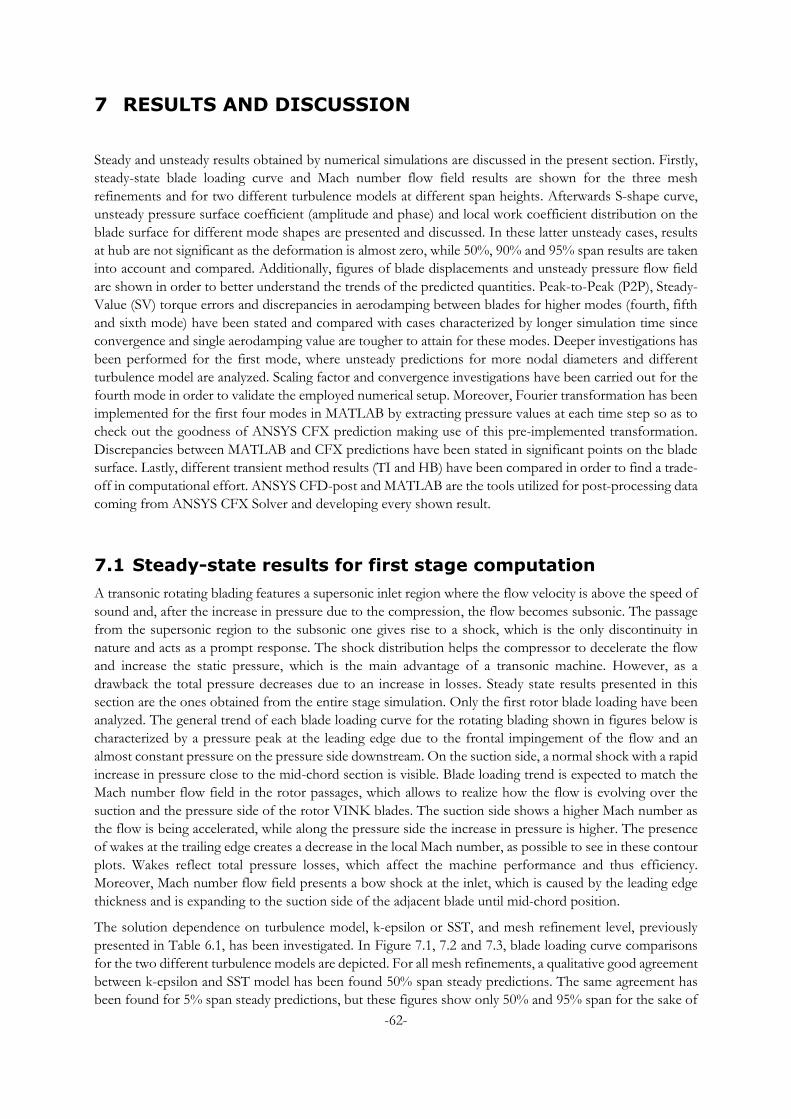
-62-
7 RESULTS AND DISCUSSION
Steady and unsteady results obtained by numerical simulations are discussed in the present section. Firstly,
steady-state blade loading curve and Mach number flow field results are shown for the three mesh
refinements and for two different turbulence models at different span heights. Afterwards S-shape curve,
unsteady pressure surface coefficient (amplitude and phase) and local work coefficient distribution on the
blade surface for different mode shapes are presented and discussed. In these latter unsteady cases, results
at hub are not significant as the deformation is almost zero, while 50%, 90% and 95% span results are taken
into account and compared. Additionally, figures of blade displacements and unsteady pressure flow field
are shown in order to better understand the trends of the predicted quantities. Peak-to-Peak (P2P), Steady-
Value (SV) torque errors and discrepancies in aerodamping between blades for higher modes (fourth, fifth
and sixth mode) have been stated and compared with cases characterized by longer simulation time since
convergence and single aerodamping value are tougher to attain for these modes. Deeper investigations has
been performed for the first mode, where unsteady predictions for more nodal diameters and different
turbulence model are analyzed. Scaling factor and convergence investigations have been carried out for the
fourth mode in order to validate the employed numerical setup. Moreover, Fourier transformation has been
implemented for the first four modes in MATLAB by extracting pressure values at each time step so as to
check out the goodness of ANSYS CFX prediction making use of this pre-implemented transformation.
Discrepancies between MATLAB and CFX predictions have been stated in significant points on the blade
surface. Lastly, different transient method results (TI and HB) have been compared in order to find a trade-
off in computational effort. ANSYS CFD-post and MATLAB are the tools utilized for post-processing data
coming from ANSYS CFX Solver and developing every shown result.
7.1 Steady-state results for first stage computation
A transonic rotating blading features a supersonic inlet region where the flow velocity is above the speed of
sound and, after the increase in pressure due to the compression, the flow becomes subsonic. The passage
from the supersonic region to the subsonic one gives rise to a shock, which is the only discontinuity in
nature and acts as a prompt response. The shock distribution helps the compressor to decelerate the flow
and increase the static pressure, which is the main advantage of a transonic machine. However, as a
drawback the total pressure decreases due to an increase in losses. Steady state results presented in this
section are the ones obtained from the entire stage simulation. Only the first rotor blade loading have been
analyzed. The general trend of each blade loading curve for the rotating blading shown in figures below is
characterized by a pressure peak at the leading edge due to the frontal impingement of the flow and an
almost constant pressure on the pressure side downstream. On the suction side, a normal shock with a rapid
increase in pressure close to the mid-chord section is visible. Blade loading trend is expected to match the
Mach number flow field in the rotor passages, which allows to realize how the flow is evolving over the
suction and the pressure side of the rotor VINK blades. The suction side shows a higher Mach number as
the flow is being accelerated, while along the pressure side the increase in pressure is higher. The presence
of wakes at the trailing edge creates a decrease in the local Mach number, as possible to see in these contour
plots. Wakes reflect total pressure losses, which affect the machine performance and thus efficiency.
Moreover, Mach number flow field presents a bow shock at the inlet, which is caused by the leading edge
thickness and is expanding to the suction side of the adjacent blade until mid-chord position.
The solution dependence on turbulence model, k-epsilon or SST, and mesh refinement level, previously
presented in Table 6.1, has been investigated. In Figure 7.1, 7.2 and 7.3, blade loading curve comparisons
for the two different turbulence models are depicted. For all mesh refinements, a qualitative good agreement
between k-epsilon and SST model has been found 50% span steady predictions. The same agreement has
been found for 5% span steady predictions, but these figures show only 50% and 95% span for the sake of
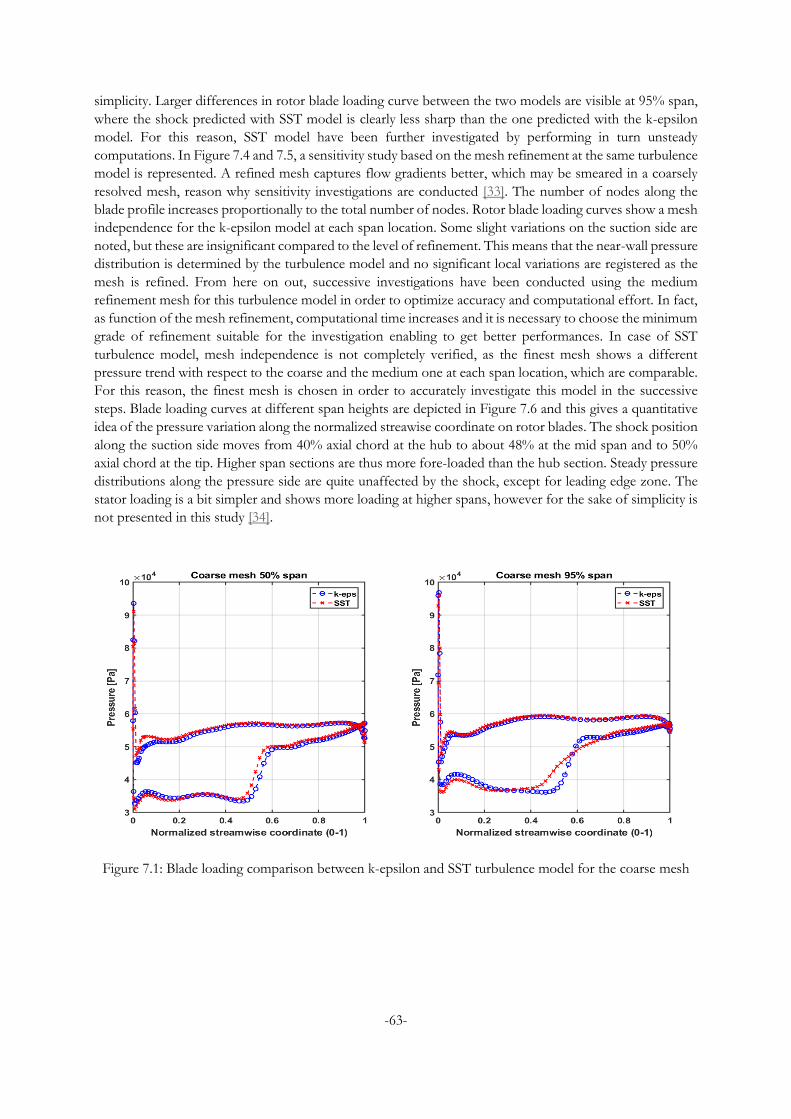
-63-
simplicity. Larger differences in rotor blade loading curve between the two models are visible at 95% span,
where the shock predicted with SST model is clearly less sharp than the one predicted with the k-epsilon
model. For this reason, SST model have been further investigated by performing in turn unsteady
computations. In Figure 7.4 and 7.5, a sensitivity study based on the mesh refinement at the same turbulence
model is represented. A refined mesh captures flow gradients better, which may be smeared in a coarsely
resolved mesh, reason why sensitivity investigations are conducted [33]. The number of nodes along the
blade profile increases proportionally to the total number of nodes. Rotor blade loading curves show a mesh
independence for the k-epsilon model at each span location. Some slight variations on the suction side are
noted, but these are insignificant compared to the level of refinement. This means that the near-wall pressure
distribution is determined by the turbulence model and no significant local variations are registered as the
mesh is refined. From here on out, successive investigations have been conducted using the medium
refinement mesh for this turbulence model in order to optimize accuracy and computational effort. In fact,
as function of the mesh refinement, computational time increases and it is necessary to choose the minimum
grade of refinement suitable for the investigation enabling to get better performances. In case of SST
turbulence model, mesh independence is not completely verified, as the finest mesh shows a different
pressure trend with respect to the coarse and the medium one at each span location, which are comparable.
For this reason, the finest mesh is chosen in order to accurately investigate this model in the successive
steps. Blade loading curves at different span heights are depicted in Figure 7.6 and this gives a quantitative
idea of the pressure variation along the normalized streawise coordinate on rotor blades. The shock position
along the suction side moves from 40% axial chord at the hub to about 48% at the mid span and to 50%
axial chord at the tip. Higher span sections are thus more fore-loaded than the hub section. Steady pressure
distributions along the pressure side are quite unaffected by the shock, except for leading edge zone. The
stator loading is a bit simpler and shows more loading at higher spans, however for the sake of simplicity is
not presented in this study [34].
Figure 7.1: Blade loading comparison between k-epsilon and SST turbulence model for the coarse mesh
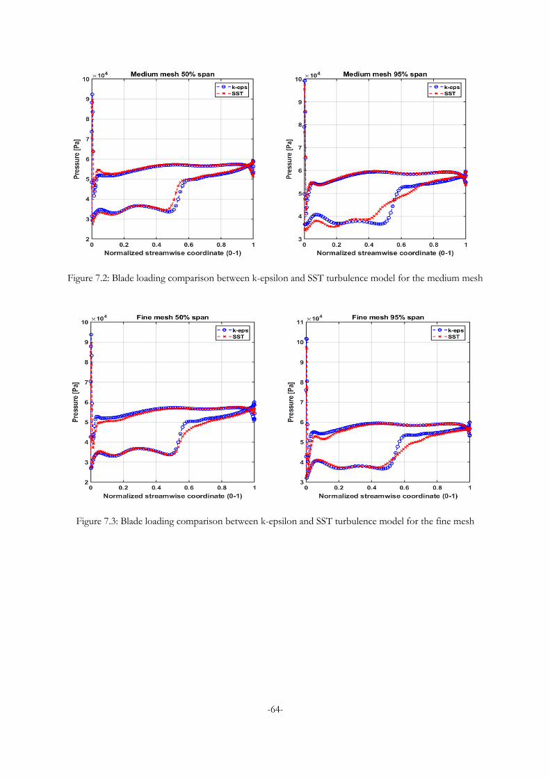
-64-
Figure 7.2: Blade loading comparison between k-epsilon and SST turbulence model for the medium mesh
Figure 7.3: Blade loading comparison between k-epsilon and SST turbulence model for the fine mesh
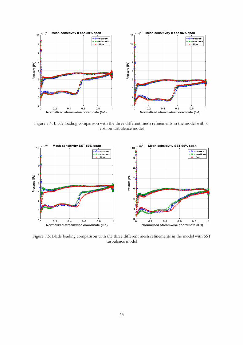
-65-
Figure 7.4: Blade loading comparison with the three different mesh refinements in the model with k-epsilon turbulence model
Figure 7.5: Blade loading comparison with the three different mesh refinements in the model with SST turbulence model
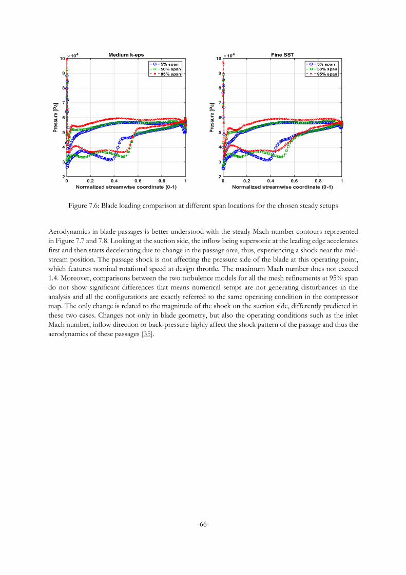
-66-
Figure 7.6: Blade loading comparison at different span locations for the chosen steady setups
Aerodynamics in blade passages is better understood with the steady Mach number contours represented
in Figure 7.7 and 7.8. Looking at the suction side, the inflow being supersonic at the leading edge accelerates
first and then starts decelerating due to change in the passage area, thus, experiencing a shock near the mid-
stream position. The passage shock is not affecting the pressure side of the blade at this operating point,
which features nominal rotational speed at design throttle. The maximum Mach number does not exceed
1.4. Moreover, comparisons between the two turbulence models for all the mesh refinements at 95% span
do not show significant differences that means numerical setups are not generating disturbances in the
analysis and all the configurations are exactly referred to the same operating condition in the compressor
map. The only change is related to the magnitude of the shock on the suction side, differently predicted in
these two cases. Changes not only in blade geometry, but also the operating conditions such as the inlet
Mach number, inflow direction or back-pressure highly affect the shock pattern of the passage and thus the
aerodynamics of these passages [35].
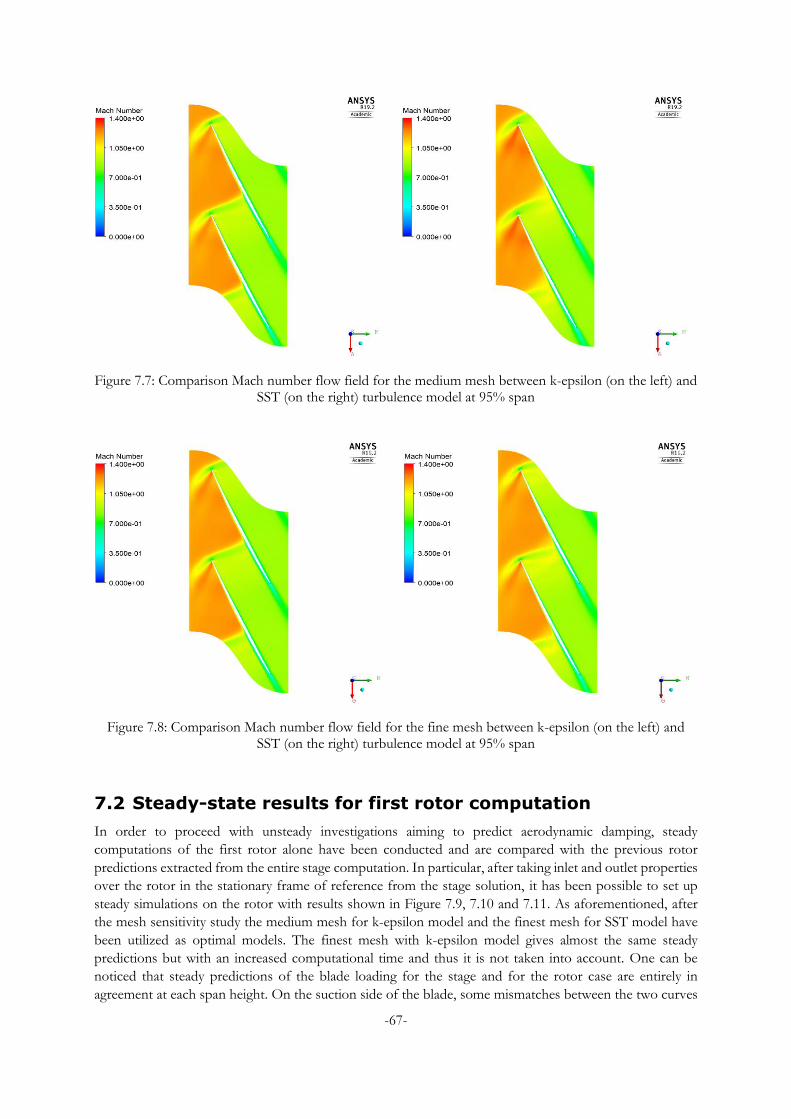
-67-
Figure 7.7: Comparison Mach number flow field for the medium mesh between k-epsilon (on the left) and SST (on the right) turbulence model at 95% span
Figure 7.8: Comparison Mach number flow field for the fine mesh between k-epsilon (on the left) and SST (on the right) turbulence model at 95% span
7.2 Steady-state results for first rotor computation
In order to proceed with unsteady investigations aiming to predict aerodynamic damping, steady
computations of the first rotor alone have been conducted and are compared with the previous rotor
predictions extracted from the entire stage computation. In particular, after taking inlet and outlet properties
over the rotor in the stationary frame of reference from the stage solution, it has been possible to set up
steady simulations on the rotor with results shown in Figure 7.9, 7.10 and 7.11. As aforementioned, after
the mesh sensitivity study the medium mesh for k-epsilon model and the finest mesh for SST model have
been utilized as optimal models. The finest mesh with k-epsilon model gives almost the same steady
predictions but with an increased computational time and thus it is not taken into account. One can be
noticed that steady predictions of the blade loading for the stage and for the rotor case are entirely in
agreement at each span height. On the suction side of the blade, some mismatches between the two curves
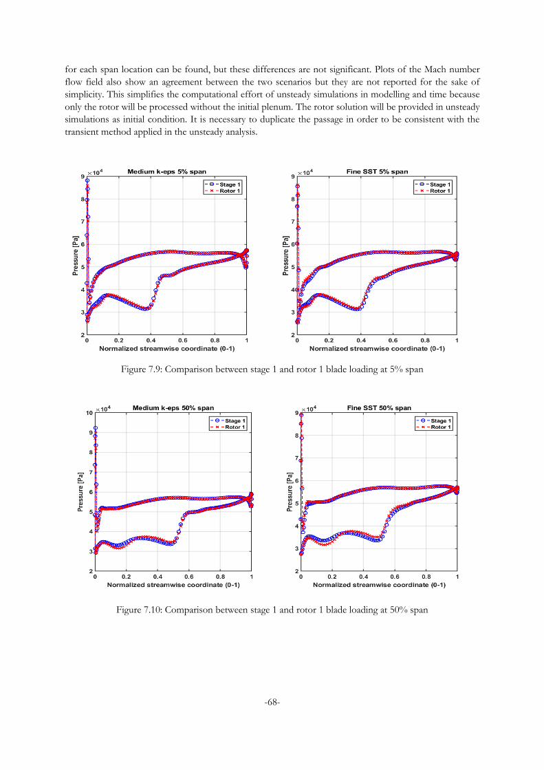
-68-
for each span location can be found, but these differences are not significant. Plots of the Mach number
flow field also show an agreement between the two scenarios but they are not reported for the sake of
simplicity. This simplifies the computational effort of unsteady simulations in modelling and time because
only the rotor will be processed without the initial plenum. The rotor solution will be provided in unsteady
simulations as initial condition. It is necessary to duplicate the passage in order to be consistent with the
transient method applied in the unsteady analysis.
Figure 7.9: Comparison between stage 1 and rotor 1 blade loading at 5% span
Figure 7.10: Comparison between stage 1 and rotor 1 blade loading at 50% span
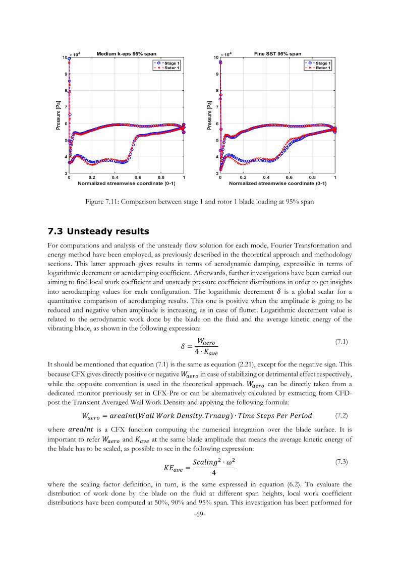
-69-
Figure 7.11: Comparison between stage 1 and rotor 1 blade loading at 95% span
7.3 Unsteady results
For computations and analysis of the unsteady flow solution for each mode, Fourier Transformation and
energy method have been employed, as previously described in the theoretical approach and methodology
sections. This latter approach gives results in terms of aerodynamic damping, expressible in terms of
logarithmic decrement or aerodamping coefficient. Afterwards, further investigations have been carried out
aiming to find local work coefficient and unsteady pressure coefficient distributions in order to get insights
into aerodamping values for each configuration. The logarithmic decrement 𝛿 is a global scalar for a
quantitative comparison of aerodamping results. This one is positive when the amplitude is going to be
reduced and negative when amplitude is increasing, as in case of flutter. Logarithmic decrement value is
related to the aerodynamic work done by the blade on the fluid and the average kinetic energy of the
vibrating blade, as shown in the following expression:
𝛿 =
𝑊𝑎𝑒𝑟𝑜4 ∙ 𝐾𝑎𝑣𝑒
(7.1)
It should be mentioned that equation (7.1) is the same as equation (2.21), except for the negative sign. This
because CFX gives directly positive or negative 𝑊𝑎𝑒𝑟𝑜 in case of stabilizing or detrimental effect respectively,
while the opposite convention is used in the theoretical approach. 𝑊𝑎𝑒𝑟𝑜 can be directly taken from a
dedicated monitor previously set in CFX-Pre or can be alternatively calculated by extracting from CFD-
post the Transient Averaged Wall Work Density and applying the following formula:
𝑊𝑎𝑒𝑟𝑜 = 𝑎𝑟𝑒𝑎𝐼𝑛𝑡(𝑊𝑎𝑙𝑙 𝑊𝑜𝑟𝑘 𝐷𝑒𝑛𝑠𝑖𝑡𝑦. 𝑇𝑟𝑛𝑎𝑣𝑔) ∙ 𝑇𝑖𝑚𝑒 𝑆𝑡𝑒𝑝𝑠 𝑃𝑒𝑟 𝑃𝑒𝑟𝑖𝑜𝑑 (7.2)
where 𝑎𝑟𝑒𝑎𝐼𝑛𝑡 is a CFX function computing the numerical integration over the blade surface. It is
important to refer 𝑊𝑎𝑒𝑟𝑜 and 𝐾𝑎𝑣𝑒 at the same blade amplitude that means the average kinetic energy of
the blade has to be scaled, as possible to see in the following expression:
𝐾𝐸𝑎𝑣𝑒 =
𝑆𝑐𝑎𝑙𝑖𝑛𝑔2 ∙ 𝜔2
4
(7.3)
where the scaling factor definition, in turn, is the same expressed in equation (6.2). To evaluate the
distribution of work done by the blade on the fluid at different span heights, local work coefficient
distributions have been computed at 50%, 90% and 95% span. This investigation has been performed for
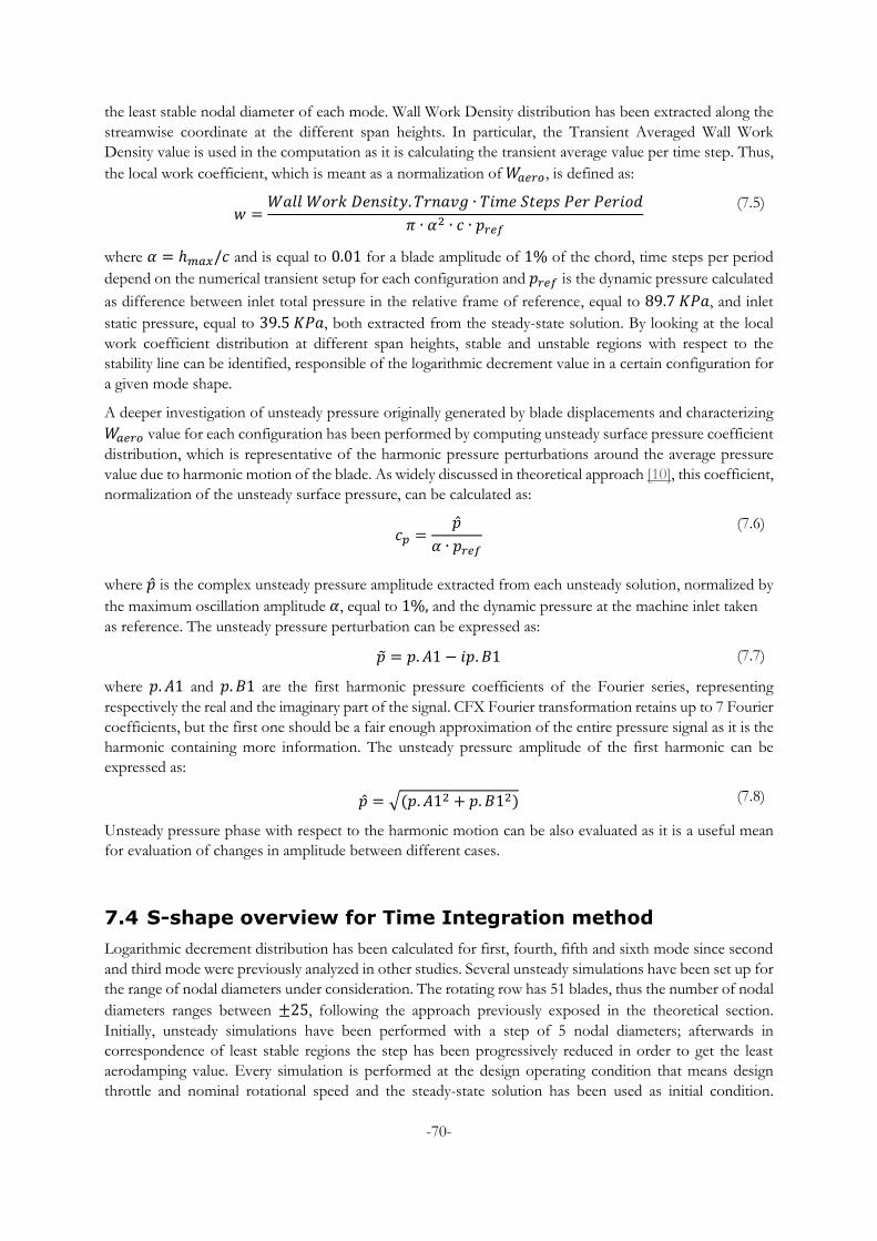
-70-
the least stable nodal diameter of each mode. Wall Work Density distribution has been extracted along the
streamwise coordinate at the different span heights. In particular, the Transient Averaged Wall Work
Density value is used in the computation as it is calculating the transient average value per time step. Thus,
the local work coefficient, which is meant as a normalization of 𝑊𝑎𝑒𝑟𝑜, is defined as:
𝑤 =
𝑊𝑎𝑙𝑙 𝑊𝑜𝑟𝑘 𝐷𝑒𝑛𝑠𝑖𝑡𝑦. 𝑇𝑟𝑛𝑎𝑣𝑔 ∙ 𝑇𝑖𝑚𝑒 𝑆𝑡𝑒𝑝𝑠 𝑃𝑒𝑟 𝑃𝑒𝑟𝑖𝑜𝑑
𝜋 ∙ 𝛼2 ∙ 𝑐 ∙ 𝑝𝑟𝑒𝑓
(7.5)
where 𝛼 = ℎ𝑚𝑎𝑥/𝑐 and is equal to 0.01 for a blade amplitude of 1% of the chord, time steps per period
depend on the numerical transient setup for each configuration and 𝑝𝑟𝑒𝑓 is the dynamic pressure calculated
as difference between inlet total pressure in the relative frame of reference, equal to 89.7 𝐾𝑃𝑎, and inlet
static pressure, equal to 39.5 𝐾𝑃𝑎, both extracted from the steady-state solution. By looking at the local
work coefficient distribution at different span heights, stable and unstable regions with respect to the
stability line can be identified, responsible of the logarithmic decrement value in a certain configuration for
a given mode shape.
A deeper investigation of unsteady pressure originally generated by blade displacements and characterizing
𝑊𝑎𝑒𝑟𝑜 value for each configuration has been performed by computing unsteady surface pressure coefficient
distribution, which is representative of the harmonic pressure perturbations around the average pressure
value due to harmonic motion of the blade. As widely discussed in theoretical approach [10], this coefficient,
normalization of the unsteady surface pressure, can be calculated as:
𝑐𝑝 =
�̂�
𝛼 ∙ 𝑝𝑟𝑒𝑓
(7.6)
where �̂� is the complex unsteady pressure amplitude extracted from each unsteady solution, normalized by
the maximum oscillation amplitude 𝛼, equal to 1%, and the dynamic pressure at the machine inlet taken
as reference. The unsteady pressure perturbation can be expressed as:
�̃� = 𝑝. 𝐴1 − 𝑖𝑝. 𝐵1 (7.7)
where 𝑝. 𝐴1 and 𝑝. 𝐵1 are the first harmonic pressure coefficients of the Fourier series, representing
respectively the real and the imaginary part of the signal. CFX Fourier transformation retains up to 7 Fourier
coefficients, but the first one should be a fair enough approximation of the entire pressure signal as it is the
harmonic containing more information. The unsteady pressure amplitude of the first harmonic can be
expressed as:
�̂� = √(𝑝. 𝐴12 + 𝑝. 𝐵12) (7.8)
Unsteady pressure phase with respect to the harmonic motion can be also evaluated as it is a useful mean
for evaluation of changes in amplitude between different cases.
7.4 S-shape overview for Time Integration method
Logarithmic decrement distribution has been calculated for first, fourth, fifth and sixth mode since second
and third mode were previously analyzed in other studies. Several unsteady simulations have been set up for
the range of nodal diameters under consideration. The rotating row has 51 blades, thus the number of nodal
diameters ranges between ±25, following the approach previously exposed in the theoretical section.
Initially, unsteady simulations have been performed with a step of 5 nodal diameters; afterwards in
correspondence of least stable regions the step has been progressively reduced in order to get the least
aerodamping value. Every simulation is performed at the design operating condition that means design
throttle and nominal rotational speed and the steady-state solution has been used as initial condition.
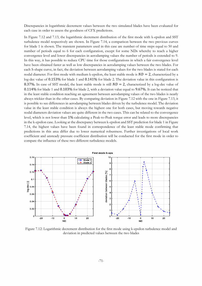
-71-
Discrepancies in logarithmic decrement values between the two simulated blades have been evaluated for
each case in order to assess the goodness of CFX predictions.
In Figure 7.12 and 7.13, the logarithmic decrement distribution of the first mode with k-epsilon and SST
turbulence model respectively are shown. In Figure 7.14, a comparison between the two previous curves
for blade 1 is shown. The transient parameters used in this case are number of time steps equal to 50 and
number of periods equal to 6 for each configuration, except for some NDs whereby to reach a higher
convergence level and lower discrepancies in aerodamping values the number of periods is extended to 9.
In this way, it has possible to reduce CPU time for those configurations in which a fair convergence level
have been obtained faster as well as low discrepancies in aerodamping values between the two blades. For
each S-shape curve, in fact, the deviation between aerodamping values for the two blades is stated for each
nodal diameter. For first mode with medium k-epsilon, the least stable mode is 𝑁𝐷 = 2, characterized by a
log-dec value of 0.153% for blade 1 and 0.141% for blade 2. The deviation value in this configuration is
8.37%. In case of SST model, the least stable mode is still 𝑁𝐷 = 2, characterized by a log-dec value of
0.114% for blade 1 and 0.103% for blade 2, with a deviation value equal to 9.67%. It can be noticed that
in the least stable condition reaching an agreement between aerodamping values of the two blades is nearly
always trickier than in the other cases. By comparing deviation in Figure 7.12 with the one in Figure 7.13, it
is possible to see differences in aerodamping between blades driven by the turbulence model. The deviation
value in the least stable condition is always the highest one for both cases, but moving towards negative
nodal diameters deviation values are quite different in the two cases. This can be related to the convergence
level, which is not lower than 1% calculating a Peak-to-Peak torque error and leads to more discrepancies
in the k-epsilon case. Looking at the discrepancy between k-epsilon and SST prediction for blade 1 in Figure
7.14, the highest values have been found in correspondence of the least stable mode confirming that
predictions in this area differ due to lower numerical robustness. Further investigations of local work
coefficient and unsteady pressure coefficient distribution will be conducted for the first mode in order to
compare the influence of these two different turbulence models.
Figure 7.12: Logarithmic decrement distribution for the first mode using k-epsilon turbulence model and deviation in predicted values between the two blades
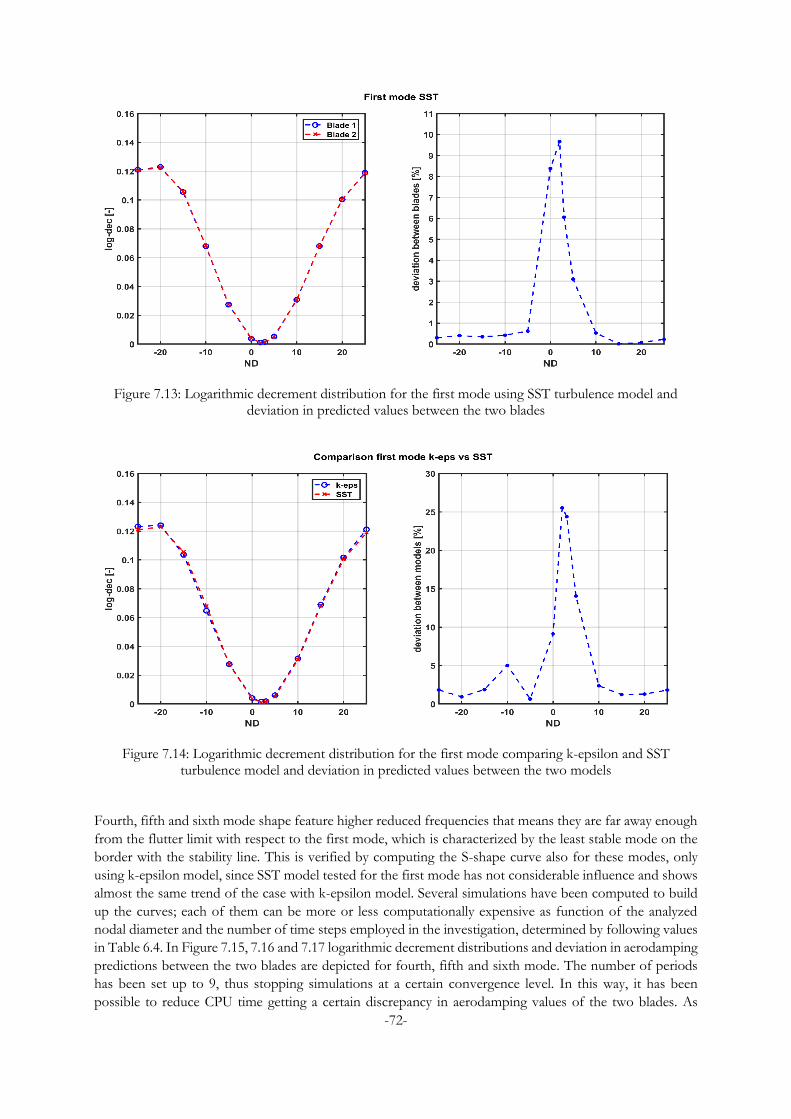
-72-
Figure 7.13: Logarithmic decrement distribution for the first mode using SST turbulence model and deviation in predicted values between the two blades
Figure 7.14: Logarithmic decrement distribution for the first mode comparing k-epsilon and SST turbulence model and deviation in predicted values between the two models
Fourth, fifth and sixth mode shape feature higher reduced frequencies that means they are far away enough
from the flutter limit with respect to the first mode, which is characterized by the least stable mode on the
border with the stability line. This is verified by computing the S-shape curve also for these modes, only
using k-epsilon model, since SST model tested for the first mode has not considerable influence and shows
almost the same trend of the case with k-epsilon model. Several simulations have been computed to build
up the curves; each of them can be more or less computationally expensive as function of the analyzed
nodal diameter and the number of time steps employed in the investigation, determined by following values
in Table 6.4. In Figure 7.15, 7.16 and 7.17 logarithmic decrement distributions and deviation in aerodamping
predictions between the two blades are depicted for fourth, fifth and sixth mode. The number of periods
has been set up to 9, thus stopping simulations at a certain convergence level. In this way, it has been
possible to reduce CPU time getting a certain discrepancy in aerodamping values of the two blades. As
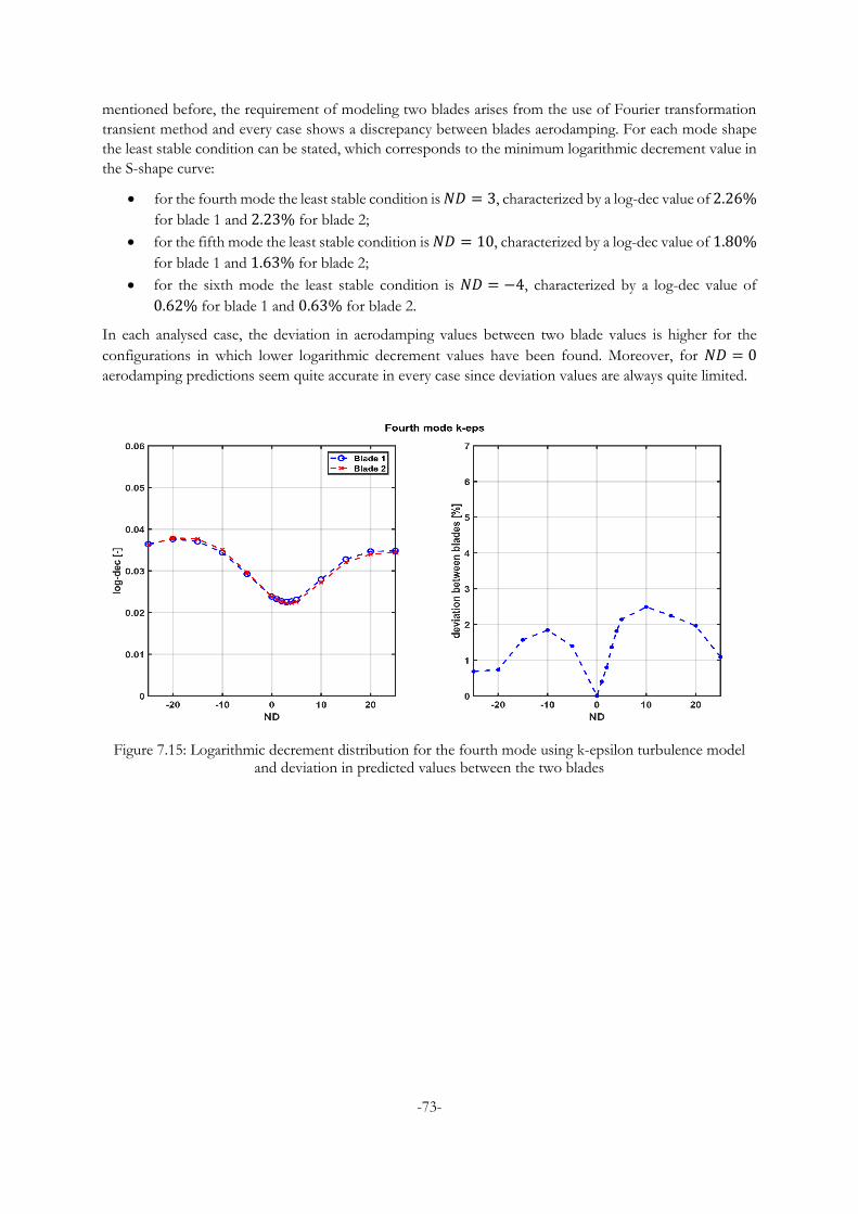
-73-
mentioned before, the requirement of modeling two blades arises from the use of Fourier transformation
transient method and every case shows a discrepancy between blades aerodamping. For each mode shape
the least stable condition can be stated, which corresponds to the minimum logarithmic decrement value in
the S-shape curve:
for the fourth mode the least stable condition is 𝑁𝐷 = 3, characterized by a log-dec value of 2.26%
for blade 1 and 2.23% for blade 2;
for the fifth mode the least stable condition is 𝑁𝐷 = 10, characterized by a log-dec value of 1.80%
for blade 1 and 1.63% for blade 2;
for the sixth mode the least stable condition is 𝑁𝐷 = −4, characterized by a log-dec value of
0.62% for blade 1 and 0.63% for blade 2.
In each analysed case, the deviation in aerodamping values between two blade values is higher for the
configurations in which lower logarithmic decrement values have been found. Moreover, for 𝑁𝐷 = 0
aerodamping predictions seem quite accurate in every case since deviation values are always quite limited.
Figure 7.15: Logarithmic decrement distribution for the fourth mode using k-epsilon turbulence model and deviation in predicted values between the two blades
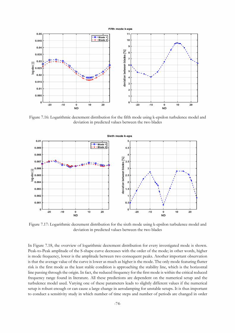
-74-
Figure 7.16: Logarithmic decrement distribution for the fifth mode using k-epsilon turbulence model and deviation in predicted values between the two blades
Figure 7.17: Logarithmic decrement distribution for the sixth mode using k-epsilon turbulence model and
deviation in predicted values between the two blades
In Figure 7.18, the overview of logarithmic decrement distribution for every investigated mode is shown.
Peak-to-Peak amplitude of the S-shape curve decreases with the order of the mode; in other words, higher
is mode frequency, lower is the amplitude between two consequent peaks. Another important observation
is that the average value of the curve is lower as much as higher is the mode. The only mode featuring flutter
risk is the first mode as the least stable condition is approaching the stability line, which is the horizontal
line passing through the origin. In fact, the reduced frequency for the first mode is within the critical reduced
frequency range found in literature. All these predictions are dependent on the numerical setup and the
turbulence model used. Varying one of these parameters leads to slightly different values if the numerical
setup is robust enough or can cause a large change in aerodamping for unstable setups. It is thus important
to conduct a sensitivity study in which number of time steps and number of periods are changed in order
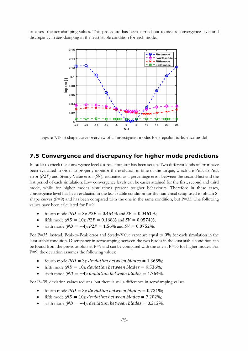
-75-
to assess the aerodamping values. This procedure has been carried out to assess convergence level and
discrepancy in aerodamping in the least stable condition for each mode.
Figure 7.18: S-shape curve overview of all investigated modes for k-epsilon turbulence model
7.5 Convergence and discrepancy for higher mode predictions
In order to check the convergence level a torque monitor has been set up. Two different kinds of error have
been evaluated in order to properly monitor the evolution in time of the torque, which are Peak-to-Peak
error (𝑃2𝑃) and Steady-Value error (𝑆𝑉), estimated as a percentage error between the second-last and the
last period of each simulation. Low convergence levels can be easier attained for the first, second and third
mode, while for higher modes simulations present tougher behaviours. Therefore in these cases,
convergence level has been evaluated in the least stable condition for the numerical setup used to obtain S-
shape curves (P=9) and has been compared with the one in the same condition, but P=35. The following
values have been calculated for P=9:
fourth mode (𝑁𝐷 = 3): 𝑃2𝑃 = 0.454% and 𝑆𝑉 = 0.0461%;
fifth mode (𝑁𝐷 = 10): 𝑃2𝑃 = 0.168% and 𝑆𝑉 = 0.0574%;
sixth mode (𝑁𝐷 = −4): 𝑃2𝑃 = 1.56% and 𝑆𝑉 = 0.0752%.
For P=35, instead, Peak-to-Peak error and Steady-Value error are equal to 0% for each simulation in the
least stable condition. Discrepancy in aerodamping between the two blades in the least stable condition can
be found from the previous plots at P=9 and can be compared with the one at P=35 for higher modes. For
P=9, the deviation assumes the following values:
fourth mode (𝑁𝐷 = 3): 𝑑𝑒𝑣𝑖𝑎𝑡𝑖𝑜𝑛 𝑏𝑒𝑡𝑤𝑒𝑒𝑛 𝑏𝑙𝑎𝑑𝑒𝑠 = 1.365%;
fifth mode (𝑁𝐷 = 10): 𝑑𝑒𝑣𝑖𝑎𝑡𝑖𝑜𝑛 𝑏𝑒𝑡𝑤𝑒𝑒𝑛 𝑏𝑙𝑎𝑑𝑒𝑠 = 9.536%;
sixth mode (𝑁𝐷 = −4): 𝑑𝑒𝑣𝑖𝑎𝑡𝑖𝑜𝑛 𝑏𝑒𝑡𝑤𝑒𝑒𝑛 𝑏𝑙𝑎𝑑𝑒𝑠 = 1.764%.
For P=35, deviation values reduces, but there is still a difference in aerodamping values:
fourth mode (𝑁𝐷 = 3): 𝑑𝑒𝑣𝑖𝑎𝑡𝑖𝑜𝑛 𝑏𝑒𝑡𝑤𝑒𝑒𝑛 𝑏𝑙𝑎𝑑𝑒𝑠 = 0.721%;
fifth mode (𝑁𝐷 = 10): 𝑑𝑒𝑣𝑖𝑎𝑡𝑖𝑜𝑛 𝑏𝑒𝑡𝑤𝑒𝑒𝑛 𝑏𝑙𝑎𝑑𝑒𝑠 = 7.202%;
sixth mode (𝑁𝐷 = −4): 𝑑𝑒𝑣𝑖𝑎𝑡𝑖𝑜𝑛 𝑏𝑒𝑡𝑤𝑒𝑒𝑛 𝑏𝑙𝑎𝑑𝑒𝑠 = 0.212%.

-76-
Therefore, it is possible to conclude that even for a Peak-to-peak error and Steady-Value error equal to 0%,
discrepancy in aerodamping values between blades is always present. This can be related to numerical error
propagations regarding reflective boundary conditions. Standard boundary conditions, when imposed on
the boundaries of an artificially truncated domain, result in reflections of the outgoing pressure waves. As
consequence, the internal domain may contain spurious wave reflections and thus it is required a precise
control of these reflections to obtain more accurate flow solutions, but no special attention has been paid
to these issues in this work.
7.6 Unsteady results for each mode
For each investigated mode and, additionally for the second and third mode taking into account only the
least stable condition stated in previous studies, unsteady pressure coefficient and local work coefficient
distribution have been computed at different span heights. In this way, it possible to get insights into the
origin of the aerodynamic damping values previously found and to have a complete overview of the force
on the blade for the first six modes. Each plot is supported with blade displacements and unsteady pressure
flow field so as to better go through these quantities. In fact, every unsteady pressure variation is led by the
displacements deforming the blade at that span location. All the modes involved in this analysis feature the
same turbulence model, which is k-epsilon. Investigations have been conducted at 50%, 90% and 95% span,
since displacements at the hub are much lower due to structural constraints and thus lower pressure
distribution as well. This study has been developed using simulation solutions with a high level of
convergence, that means P=9 for the first mode, P=14 for second and third mode and P=35 for the higher
modes.
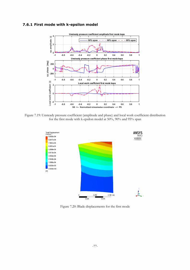
-77-
7.6.1 First mode with k-epsilon model
Figure 7.19: Unsteady pressure coefficient (amplitude and phase) and local work coefficient distribution for the first mode with k-epsilon model at 50%, 90% and 95% span
Figure 7.20: Blade displacements for the first mode
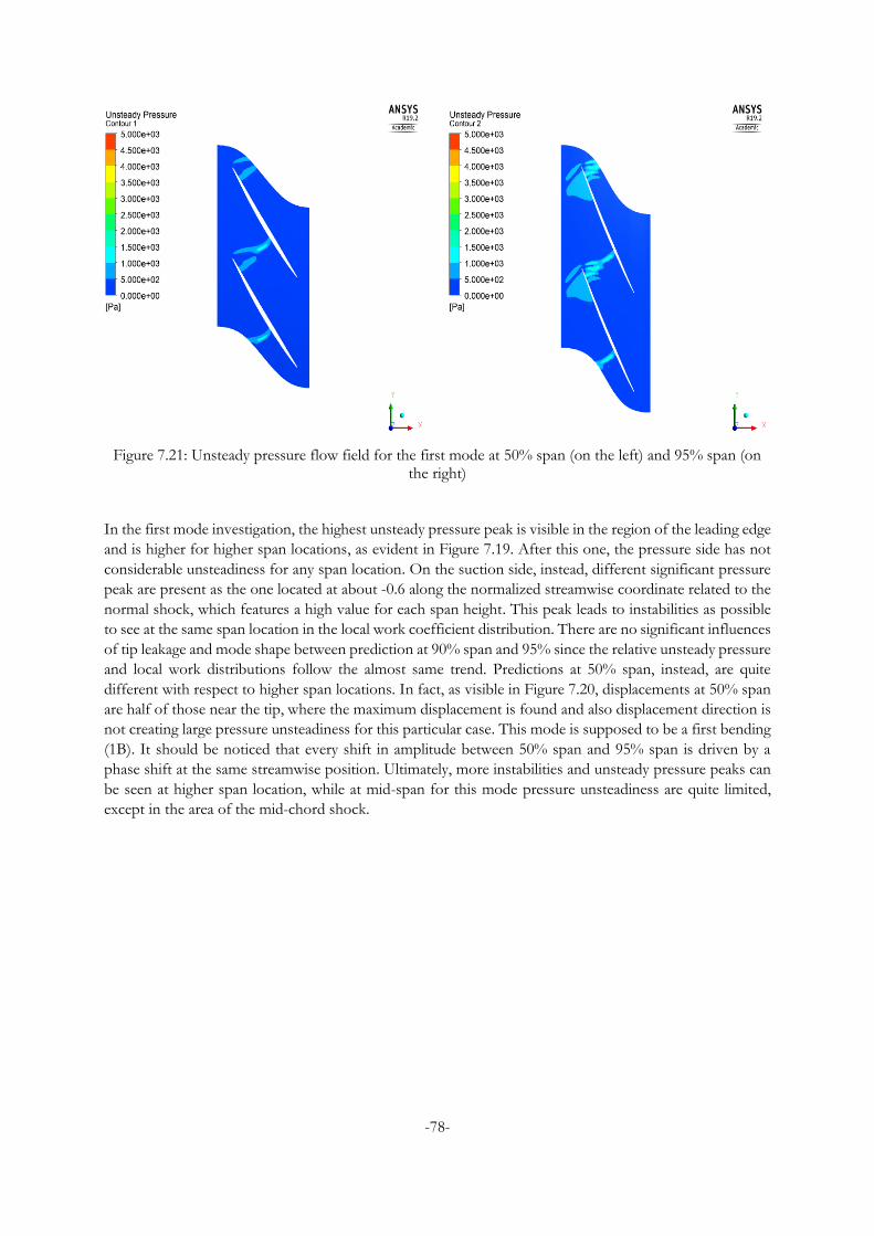
-78-
Figure 7.21: Unsteady pressure flow field for the first mode at 50% span (on the left) and 95% span (on the right)
In the first mode investigation, the highest unsteady pressure peak is visible in the region of the leading edge
and is higher for higher span locations, as evident in Figure 7.19. After this one, the pressure side has not
considerable unsteadiness for any span location. On the suction side, instead, different significant pressure
peak are present as the one located at about -0.6 along the normalized streamwise coordinate related to the
normal shock, which features a high value for each span height. This peak leads to instabilities as possible
to see at the same span location in the local work coefficient distribution. There are no significant influences
of tip leakage and mode shape between prediction at 90% span and 95% since the relative unsteady pressure
and local work distributions follow the almost same trend. Predictions at 50% span, instead, are quite
different with respect to higher span locations. In fact, as visible in Figure 7.20, displacements at 50% span
are half of those near the tip, where the maximum displacement is found and also displacement direction is
not creating large pressure unsteadiness for this particular case. This mode is supposed to be a first bending
(1B). It should be noticed that every shift in amplitude between 50% span and 95% span is driven by a
phase shift at the same streamwise position. Ultimately, more instabilities and unsteady pressure peaks can
be seen at higher span location, while at mid-span for this mode pressure unsteadiness are quite limited,
except in the area of the mid-chord shock.
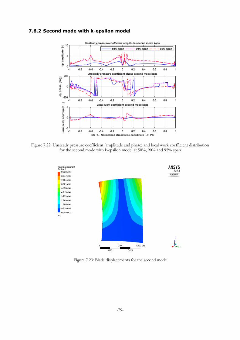
-79-
7.6.2 Second mode with k-epsilon model
Figure 7.22: Unsteady pressure coefficient (amplitude and phase) and local work coefficient distribution for the second mode with k-epsilon model at 50%, 90% and 95% span
Figure 7.23: Blade displacements for the second mode
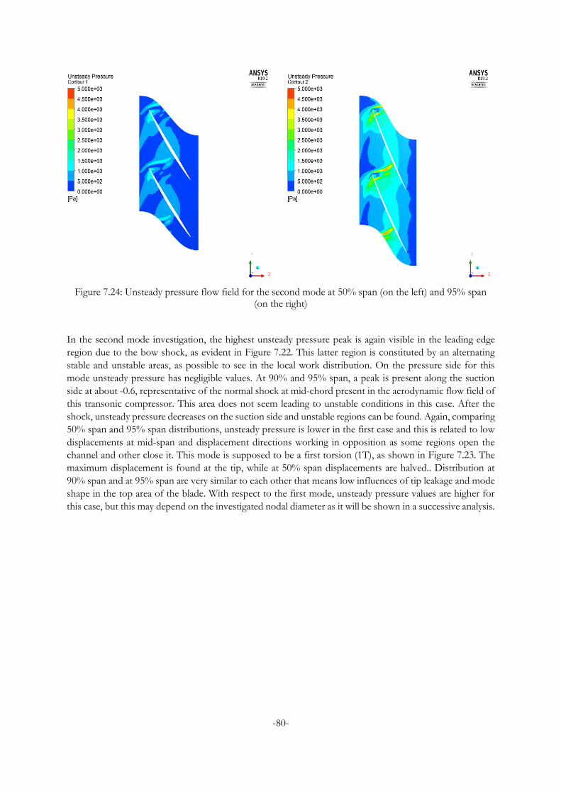
-80-
Figure 7.24: Unsteady pressure flow field for the second mode at 50% span (on the left) and 95% span (on the right)
In the second mode investigation, the highest unsteady pressure peak is again visible in the leading edge
region due to the bow shock, as evident in Figure 7.22. This latter region is constituted by an alternating
stable and unstable areas, as possible to see in the local work distribution. On the pressure side for this
mode unsteady pressure has negligible values. At 90% and 95% span, a peak is present along the suction
side at about -0.6, representative of the normal shock at mid-chord present in the aerodynamic flow field of
this transonic compressor. This area does not seem leading to unstable conditions in this case. After the
shock, unsteady pressure decreases on the suction side and unstable regions can be found. Again, comparing
50% span and 95% span distributions, unsteady pressure is lower in the first case and this is related to low
displacements at mid-span and displacement directions working in opposition as some regions open the
channel and other close it. This mode is supposed to be a first torsion (1T), as shown in Figure 7.23. The
maximum displacement is found at the tip, while at 50% span displacements are halved.. Distribution at
90% span and at 95% span are very similar to each other that means low influences of tip leakage and mode
shape in the top area of the blade. With respect to the first mode, unsteady pressure values are higher for
this case, but this may depend on the investigated nodal diameter as it will be shown in a successive analysis.
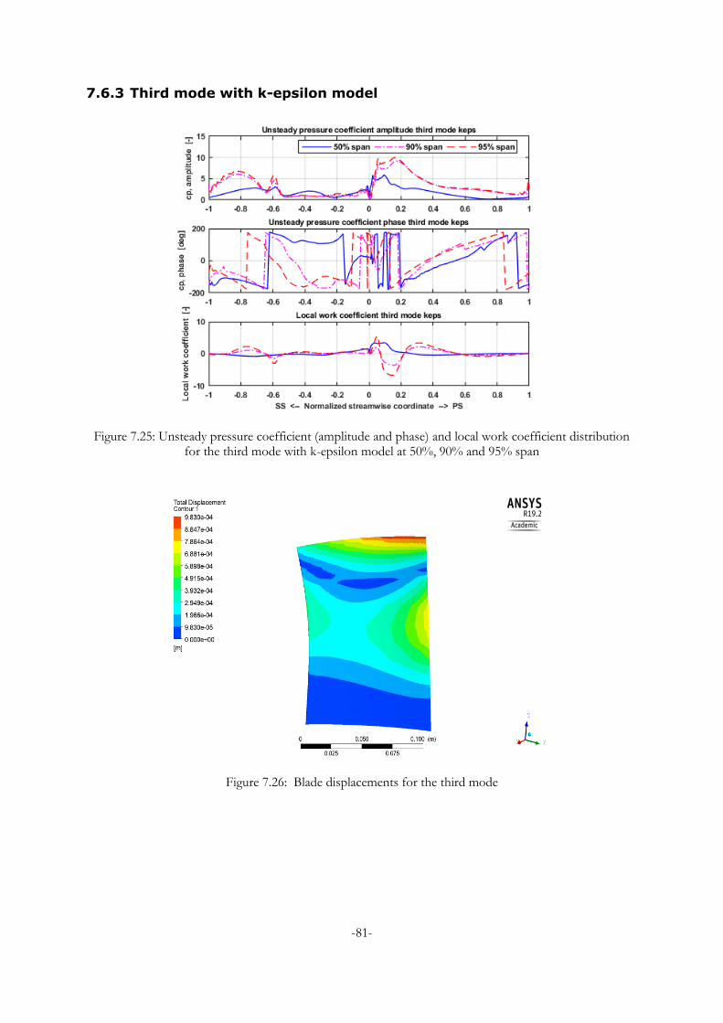
-81-
7.6.3 Third mode with k-epsilon model
Figure 7.25: Unsteady pressure coefficient (amplitude and phase) and local work coefficient distribution for the third mode with k-epsilon model at 50%, 90% and 95% span
Figure 7.26: Blade displacements for the third mode
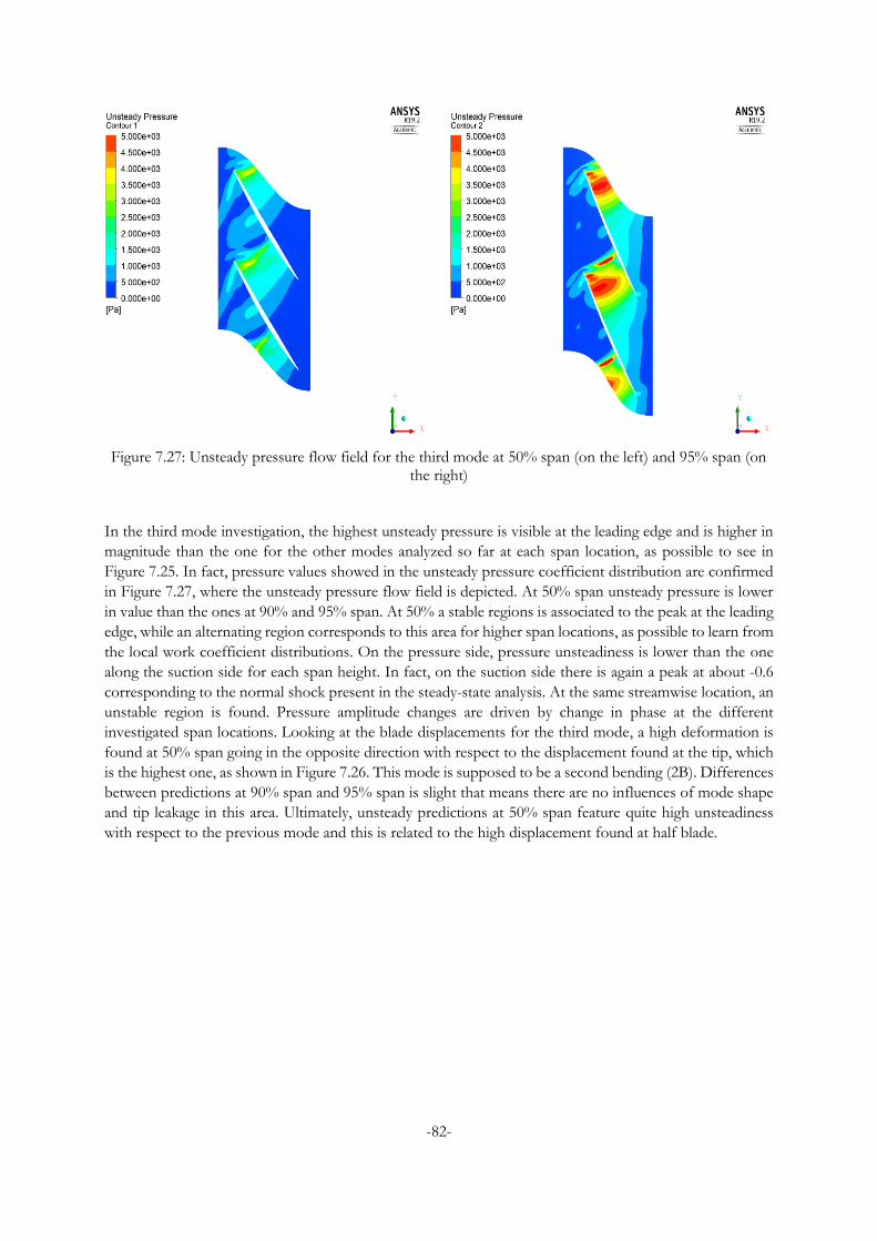
-82-
Figure 7.27: Unsteady pressure flow field for the third mode at 50% span (on the left) and 95% span (on the right)
In the third mode investigation, the highest unsteady pressure is visible at the leading edge and is higher in
magnitude than the one for the other modes analyzed so far at each span location, as possible to see in
Figure 7.25. In fact, pressure values showed in the unsteady pressure coefficient distribution are confirmed
in Figure 7.27, where the unsteady pressure flow field is depicted. At 50% span unsteady pressure is lower
in value than the ones at 90% and 95% span. At 50% a stable regions is associated to the peak at the leading
edge, while an alternating region corresponds to this area for higher span locations, as possible to learn from
the local work coefficient distributions. On the pressure side, pressure unsteadiness is lower than the one
along the suction side for each span height. In fact, on the suction side there is again a peak at about -0.6
corresponding to the normal shock present in the steady-state analysis. At the same streamwise location, an
unstable region is found. Pressure amplitude changes are driven by change in phase at the different
investigated span locations. Looking at the blade displacements for the third mode, a high deformation is
found at 50% span going in the opposite direction with respect to the displacement found at the tip, which
is the highest one, as shown in Figure 7.26. This mode is supposed to be a second bending (2B). Differences
between predictions at 90% span and 95% span is slight that means there are no influences of mode shape
and tip leakage in this area. Ultimately, unsteady predictions at 50% span feature quite high unsteadiness
with respect to the previous mode and this is related to the high displacement found at half blade.
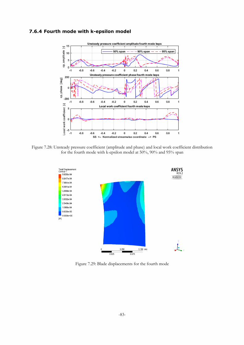
-83-
7.6.4 Fourth mode with k-epsilon model
Figure 7.28: Unsteady pressure coefficient (amplitude and phase) and local work coefficient distribution for the fourth mode with k-epsilon model at 50%, 90% and 95% span
Figure 7.29: Blade displacements for the fourth mode
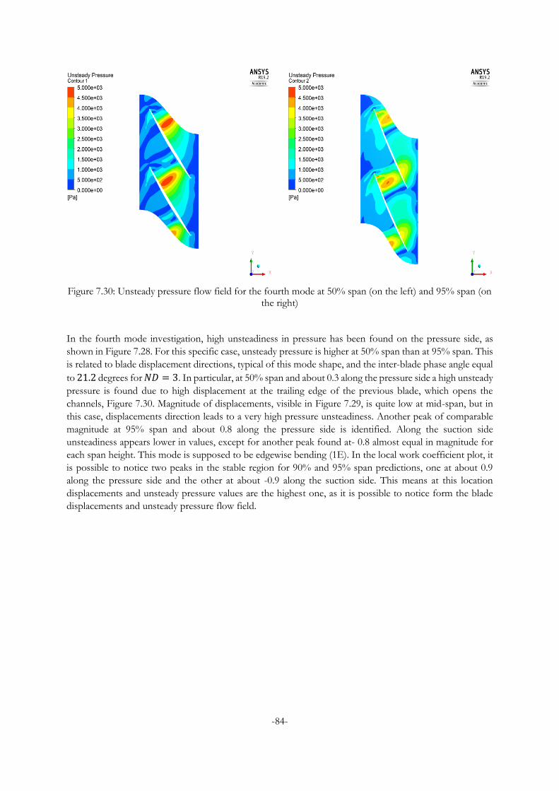
-84-
Figure 7.30: Unsteady pressure flow field for the fourth mode at 50% span (on the left) and 95% span (on the right)
In the fourth mode investigation, high unsteadiness in pressure has been found on the pressure side, as
shown in Figure 7.28. For this specific case, unsteady pressure is higher at 50% span than at 95% span. This
is related to blade displacement directions, typical of this mode shape, and the inter-blade phase angle equal
to 21.2 degrees for 𝑁𝐷 = 3. In particular, at 50% span and about 0.3 along the pressure side a high unsteady
pressure is found due to high displacement at the trailing edge of the previous blade, which opens the
channels, Figure 7.30. Magnitude of displacements, visible in Figure 7.29, is quite low at mid-span, but in
this case, displacements direction leads to a very high pressure unsteadiness. Another peak of comparable
magnitude at 95% span and about 0.8 along the pressure side is identified. Along the suction side
unsteadiness appears lower in values, except for another peak found at- 0.8 almost equal in magnitude for
each span height. This mode is supposed to be edgewise bending (1E). In the local work coefficient plot, it
is possible to notice two peaks in the stable region for 90% and 95% span predictions, one at about 0.9
along the pressure side and the other at about -0.9 along the suction side. This means at this location
displacements and unsteady pressure values are the highest one, as it is possible to notice form the blade
displacements and unsteady pressure flow field.
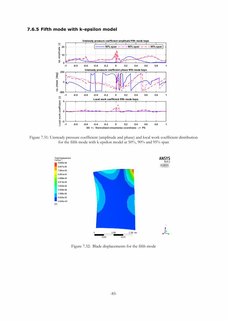
-85-
7.6.5 Fifth mode with k-epsilon model
Figure 7.31: Unsteady pressure coefficient (amplitude and phase) and local work coefficient distribution for the fifth mode with k-epsilon model at 50%, 90% and 95% span
Figure 7.32: Blade displacements for the fifth mode
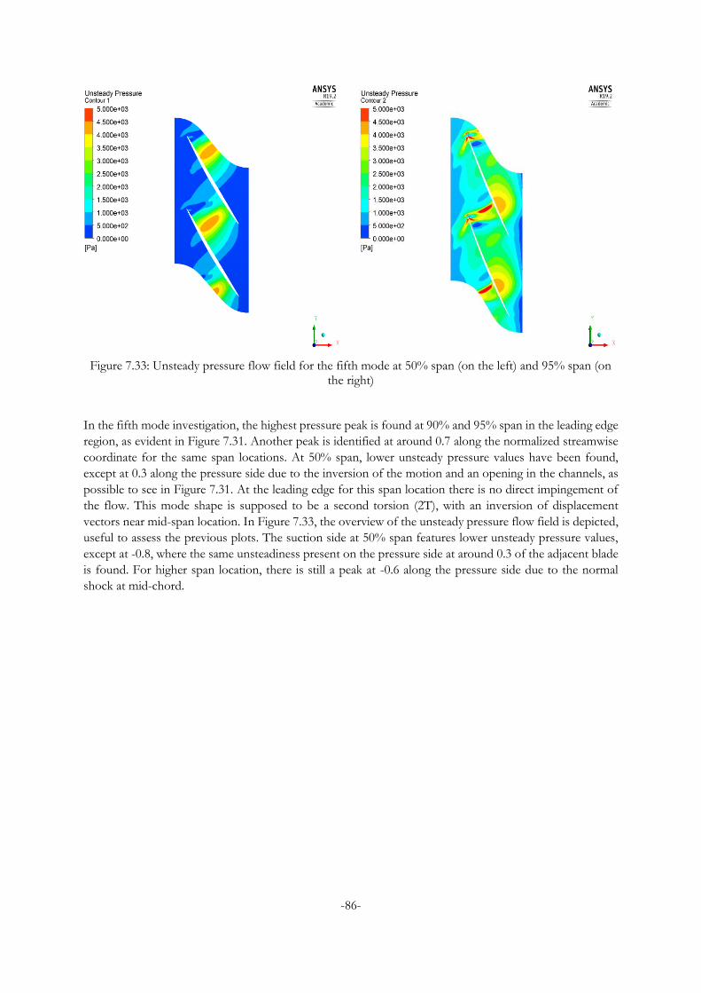
-86-
Figure 7.33: Unsteady pressure flow field for the fifth mode at 50% span (on the left) and 95% span (on the right)
In the fifth mode investigation, the highest pressure peak is found at 90% and 95% span in the leading edge
region, as evident in Figure 7.31. Another peak is identified at around 0.7 along the normalized streamwise
coordinate for the same span locations. At 50% span, lower unsteady pressure values have been found,
except at 0.3 along the pressure side due to the inversion of the motion and an opening in the channels, as
possible to see in Figure 7.31. At the leading edge for this span location there is no direct impingement of
the flow. This mode shape is supposed to be a second torsion (2T), with an inversion of displacement
vectors near mid-span location. In Figure 7.33, the overview of the unsteady pressure flow field is depicted,
useful to assess the previous plots. The suction side at 50% span features lower unsteady pressure values,
except at -0.8, where the same unsteadiness present on the pressure side at around 0.3 of the adjacent blade
is found. For higher span location, there is still a peak at -0.6 along the pressure side due to the normal
shock at mid-chord.
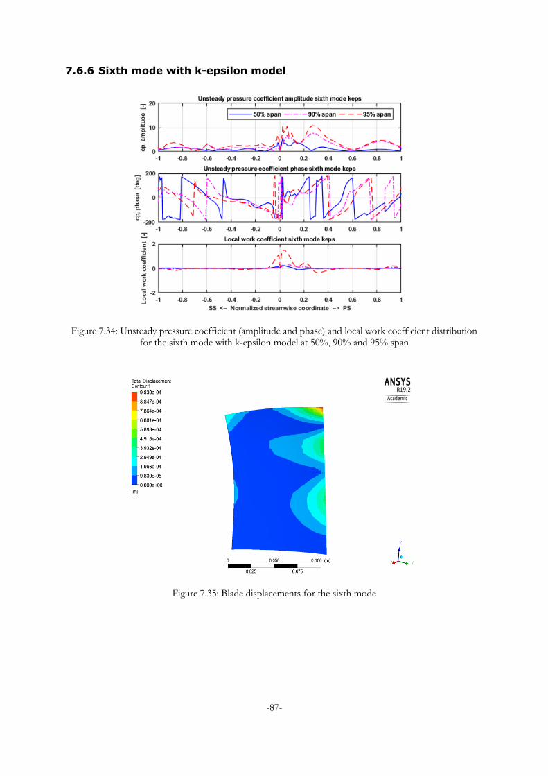
-87-
7.6.6 Sixth mode with k-epsilon model
Figure 7.34: Unsteady pressure coefficient (amplitude and phase) and local work coefficient distribution for the sixth mode with k-epsilon model at 50%, 90% and 95% span
Figure 7.35: Blade displacements for the sixth mode
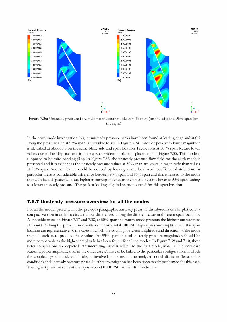
-88-
Figure 7.36: Unsteady pressure flow field for the sixth mode at 50% span (on the left) and 95% span (on the right)
In the sixth mode investigation, higher unsteady pressure peaks have been found at leading edge and at 0.3
along the pressure side at 95% span, as possible to see in Figure 7.34. Another peak with lower magnitude
is identified at about 0.8 on the same blade side and span location. Predictions at 50 % span feature lower
values due to low displacement in this case, as evident in blade displacements in Figure 7.35. This mode is
supposed to be third bending (3B). In Figure 7.36, the unsteady pressure flow field for the sixth mode is
presented and it is evident as the unsteady pressure values at 50% span are lower in magnitude than values
at 95% span. Another feature could be noticed by looking at the local work coefficient distribution. In
particular there is considerable difference between 90% span and 95% span and this is related to the mode
shape. In fact, displacements are higher in correspondence of the tip and become lower at 90% span leading
to a lower unsteady pressure. The peak at leading edge is less pronounced for this span location.
7.6.7 Unsteady pressure overview for all the modes
For all the modes presented in the previous paragraphs, unsteady pressure distributions can be plotted in a
compact version in order to discuss about differences among the different cases at different span locations.
As possible to see in Figure 7.37 and 7.38, at 50% span the fourth mode presents the highest unsteadiness
at about 0.3 along the pressure side, with a value around 4500 𝑃𝑎. Higher pressure amplitudes at this span
location are representative of the cases in which the coupling between amplitude and direction of the mode
shape is such as to produce these values. At 95% span, instead unsteady pressure magnitudes should be
more comparable as the highest amplitude has been found for all the modes. In Figure 7.39 and 7.40, these
latter comparisons are depicted. An interesting issue is related to the first mode, which is the only case
featuring lower amplitude than in the other cases. This can be linked to the particular configuration, in which
the coupled system, disk and blade, is involved, in terms of the analyzed nodal diameter (least stable
condition) and unsteady pressure phase. Further investigation has been successively performed for this case.
The highest pressure value at the tip is around 8000 𝑃𝑎 for the fifth mode case.
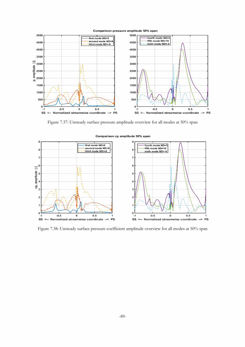
-89-
Figure 7.37: Unsteady surface pressure amplitude overview for all modes at 50% span
Figure 7.38: Unsteady surface pressure coefficient amplitude overview for all modes at 50% span
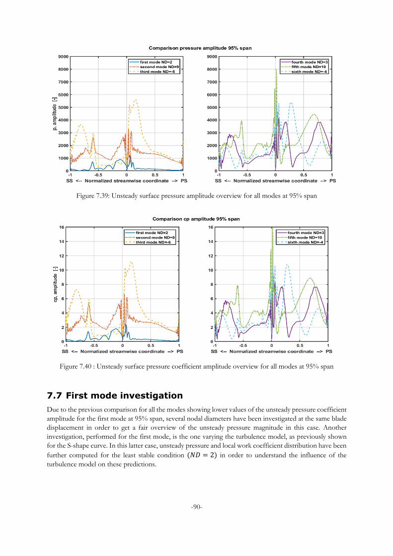
-90-
Figure 7.39: Unsteady surface pressure amplitude overview for all modes at 95% span
Figure 7.40 : Unsteady surface pressure coefficient amplitude overview for all modes at 95% span
7.7 First mode investigation
Due to the previous comparison for all the modes showing lower values of the unsteady pressure coefficient
amplitude for the first mode at 95% span, several nodal diameters have been investigated at the same blade
displacement in order to get a fair overview of the unsteady pressure magnitude in this case. Another
investigation, performed for the first mode, is the one varying the turbulence model, as previously shown
for the S-shape curve. In this latter case, unsteady pressure and local work coefficient distribution have been
further computed for the least stable condition (𝑁𝐷 = 2) in order to understand the influence of the
turbulence model on these predictions.
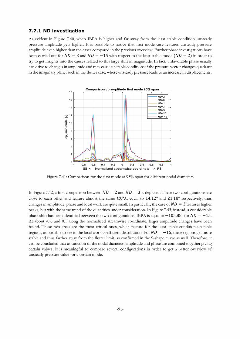
-91-
7.7.1 ND investigation
As evident in Figure 7.40, when IBPA is higher and far away from the least stable condition unsteady
pressure amplitude gets higher. It is possible to notice that first mode case features unsteady pressure
amplitude even higher than the cases compared in the previous overview. Further phase investigations have
been carried out for 𝑁𝐷 = 3 and 𝑁𝐷 = −15 with respect to the least stable mode (𝑁𝐷 = 2) in order to
try to get insights into the causes related to this large shift in magnitude. In fact, unfavorable phase usually
can drive to changes in amplitude and may cause unstable conditions if the pressure vector changes quadrant
in the imaginary plane, such in the flutter case, where unsteady pressure leads to an increase in displacements.
Figure 7.41: Comparison for the first mode at 95% span for different nodal diameters
In Figure 7.42, a first comparison between 𝑁𝐷 = 2 and 𝑁𝐷 = 3 is depicted. These two configurations are
close to each other and feature almost the same 𝐼𝐵𝑃𝐴, equal to 14.12° and 21.18° respectively; thus
changes in amplitude, phase and local work are quite small. In particular, the case of 𝑁𝐷 = 3 features higher
peaks, but with the same trend of the quantities under consideration. In Figure 7.43, instead, a considerable
phase shift has been identified between the two configurations. IBPA is equal to −105.88° for 𝑁𝐷 = −15.
At about -0.6 and 0.1 along the normalized streamwise coordinate, larger amplitude changes have been
found. These two areas are the most critical ones, which feature for the least stable condition unstable
regions, as possible to see in the local work coefficient distribution. For 𝑁𝐷 = −15, these regions get more
stable and thus farther away from the flutter limit, as confirmed in the S-shape curve as well. Therefore, it
can be concluded that as function of the nodal diameter, amplitude and phase are combined together giving
certain values; it is meaningful to compare several configurations in order to get a better overview of
unsteady pressure value for a certain mode.
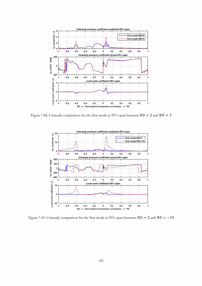
-92-
Figure 7.42: Unsteady comparison for the first mode at 95% span between 𝑁𝐷 = 2 and 𝑁𝐷 = 3
Figure 7.43: Unsteady comparison for the first mode at 95% span between 𝑁𝐷 = 2 and 𝑁𝐷 = −15
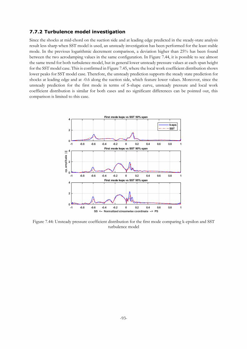
-93-
7.7.2 Turbulence model investigation
Since the shocks at mid-chord on the suction side and at leading edge predicted in the steady-state analysis
result less sharp when SST model is used, an unsteady investigation has been performed for the least stable
mode. In the previous logarithmic decrement comparison, a deviation higher than 25% has been found
between the two aerodamping values in the same configuration. In Figure 7.44, it is possible to see almost
the same trend for both turbulence model, but in general lower unsteady pressure values at each span height
for the SST model case. This is confirmed in Figure 7.45, where the local work coefficient distribution shows
lower peaks for SST model case. Therefore, the unsteady prediction supports the steady state prediction for
shocks at leading edge and at -0.6 along the suction side, which feature lower values. Moreover, since the
unsteady prediction for the first mode in terms of S-shape curve, unsteady pressure and local work
coefficient distribution is similar for both cases and no significant differences can be pointed out, this
comparison is limited to this case.
Figure 7.44: Unsteady pressure coefficient distribution for the first mode comparing k-epsilon and SST turbulence model
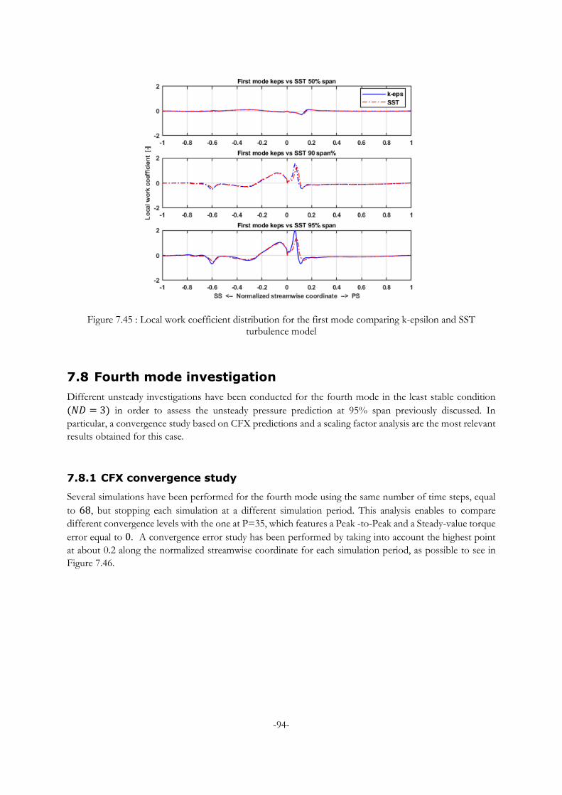
-94-
Figure 7.45 : Local work coefficient distribution for the first mode comparing k-epsilon and SST turbulence model
7.8 Fourth mode investigation
Different unsteady investigations have been conducted for the fourth mode in the least stable condition
(𝑁𝐷 = 3) in order to assess the unsteady pressure prediction at 95% span previously discussed. In
particular, a convergence study based on CFX predictions and a scaling factor analysis are the most relevant
results obtained for this case.
7.8.1 CFX convergence study
Several simulations have been performed for the fourth mode using the same number of time steps, equal
to 68, but stopping each simulation at a different simulation period. This analysis enables to compare
different convergence levels with the one at P=35, which features a Peak -to-Peak and a Steady-value torque
error equal to 0. A convergence error study has been performed by taking into account the highest point
at about 0.2 along the normalized streamwise coordinate for each simulation period, as possible to see in
Figure 7.46.
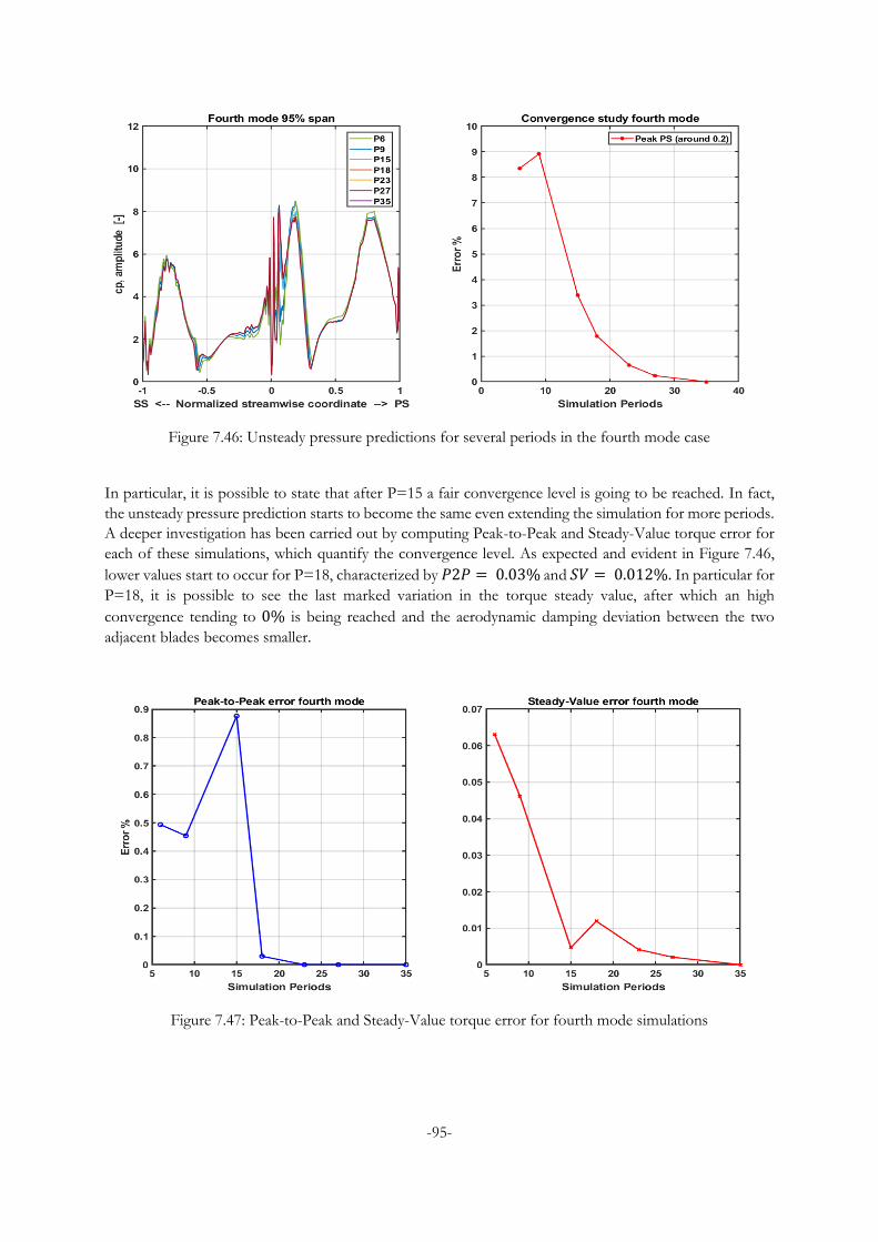
-95-
Figure 7.46: Unsteady pressure predictions for several periods in the fourth mode case
In particular, it is possible to state that after P=15 a fair convergence level is going to be reached. In fact,
the unsteady pressure prediction starts to become the same even extending the simulation for more periods.
A deeper investigation has been carried out by computing Peak-to-Peak and Steady-Value torque error for
each of these simulations, which quantify the convergence level. As expected and evident in Figure 7.46,
lower values start to occur for P=18, characterized by 𝑃2𝑃 = 0.03% and 𝑆𝑉 = 0.012%. In particular for
P=18, it is possible to see the last marked variation in the torque steady value, after which an high
convergence tending to 0% is being reached and the aerodynamic damping deviation between the two
adjacent blades becomes smaller.
Figure 7.47: Peak-to-Peak and Steady-Value torque error for fourth mode simulations
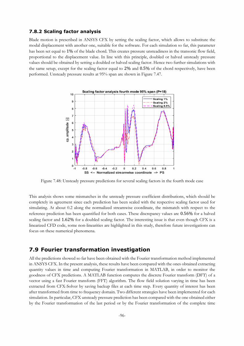
-96-
7.8.2 Scaling factor analysis
Blade motion is prescribed in ANSYS CFX by setting the scaling factor, which allows to substitute the
modal displacement with another one, suitable for the software. For each simulation so far, this parameter
has been set equal to 1% of the blade chord. This creates pressure unsteadiness in the transonic flow field,
proportional to the displacement value. In line with this principle, doubled or halved unsteady pressure
values should be obtained by setting a doubled or halved scaling factor. Hence two further simulations with
the same setup, except for the scaling factor equal to 2% and 0.5% of the chord respectively, have been
performed. Unsteady pressure results at 95% span are shown in Figure 7.47.
Figure 7.48: Unsteady pressure predictions for several scaling factors in the fourth mode case
This analysis shows some mismatches in the unsteady pressure coefficient distributions, which should be
completely in agreement since each prediction has been scaled with the respective scaling factor used for
simulating. At about 0.2 along the normalized streamwise coordinate, the mismatch with respect to the
reference prediction has been quantified for both cases. These discrepancy values are 0.56% for a halved
scaling factor and 1.62% for a doubled scaling factor. The interesting issue is that even though CFX is a
linearized CFD code, some non-linearities are highlighted in this study, therefore future investigations can
focus on these numerical phenomena.
7.9 Fourier transformation investigation
All the predictions showed so far have been obtained with the Fourier transformation method implemented
in ANSYS CFX. In the present analysis, these results have been compared with the ones obtained extracting
quantity values in time and computing Fourier transformation in MATLAB, in order to monitor the
goodness of CFX predictions. A MATLAB function computes the discrete Fourier transform (DFT) of a
vector using a fast Fourier transform (FFT) algorithm. The flow field solution varying in time has been
extracted from CFX-Solver by saving backup files at each time step. Every quantity of interest has been
after transformed from time to frequency domain. Two different strategies have been implemented for each
simulation. In particular, CFX unsteady pressure prediction has been compared with the one obtained either
by the Fourier transformation of the last period or by the Fourier transformation of the complete time
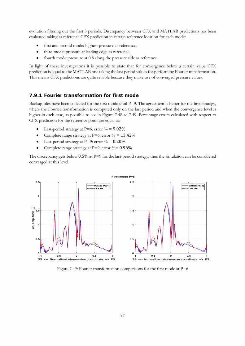
-97-
evolution filtering out the first 3 periods. Discrepancy between CFX and MATLAB predictions has been
evaluated taking as reference CFX prediction in certain reference location for each mode:
first and second mode: highest pressure as reference;
third mode: pressure at leading edge as reference;
fourth mode: pressure at 0.8 along the pressure side as reference.
In light of these investigations it is possible to state that for convergence below a certain value CFX
prediction is equal to the MATLAB one taking the last period values for performing Fourier transformation.
This means CFX predictions are quite reliable because they make use of converged pressure values.
7.9.1 Fourier transformation for first mode
Backup files have been collected for the first mode until P=9. The agreement is better for the first strategy,
where the Fourier transformation is computed only on the last period and when the convergence level is
higher in each case, as possible to see in Figure 7.48 ad 7.49. Percentage errors calculated with respect to
CFX prediction for the reference point are equal to:
Last-period strategy at P=6: error % = 9.02%
Complete range strategy at P=6: error % = 13.42%
Last-period strategy at P=9: error % = 0.20%
Complete range strategy at P=9: error %= 0.96%
The discrepancy gets below 0.5% at P=9 for the last-period strategy, thus the simulation can be considered
converged at this level.
Figure 7.49: Fourier transformation comparisons for the first mode at P=6
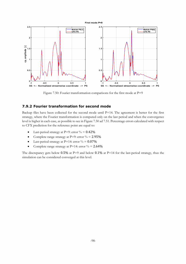
-98-
Figure 7.50: Fourier transformation comparisons for the first mode at P=9
7.9.2 Fourier transformation for second mode
Backup files have been collected for the second mode until P=14. The agreement is better for the first
strategy, where the Fourier transformation is computed only on the last period and when the convergence
level is higher in each case, as possible to see in Figure 7.50 ad 7.51. Percentage errors calculated with respect
to CFX prediction for the reference point are equal to:
Last-period strategy at P=9: error % = 0.42%
Complete range strategy at P=9: error % = 2.95%
Last-period strategy at P=14: error % = 0.07%
Complete range strategy at P=14: error % = 2.64%
The discrepancy gets below 0.5% at P=9 and below 0.1% at P=14 for the last-period strategy, thus the
simulation can be considered converged at this level.
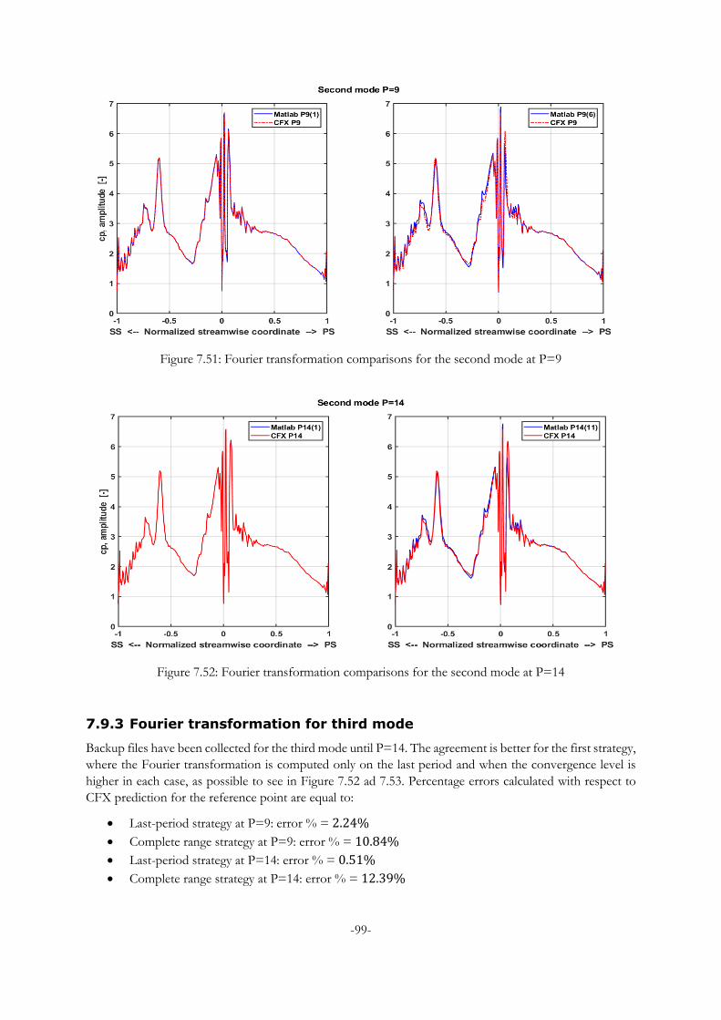
-99-
Figure 7.51: Fourier transformation comparisons for the second mode at P=9
Figure 7.52: Fourier transformation comparisons for the second mode at P=14
7.9.3 Fourier transformation for third mode
Backup files have been collected for the third mode until P=14. The agreement is better for the first strategy,
where the Fourier transformation is computed only on the last period and when the convergence level is
higher in each case, as possible to see in Figure 7.52 ad 7.53. Percentage errors calculated with respect to
CFX prediction for the reference point are equal to:
Last-period strategy at P=9: error % = 2.24%
Complete range strategy at P=9: error % = 10.84%
Last-period strategy at P=14: error % = 0.51%
Complete range strategy at P=14: error % = 12.39%
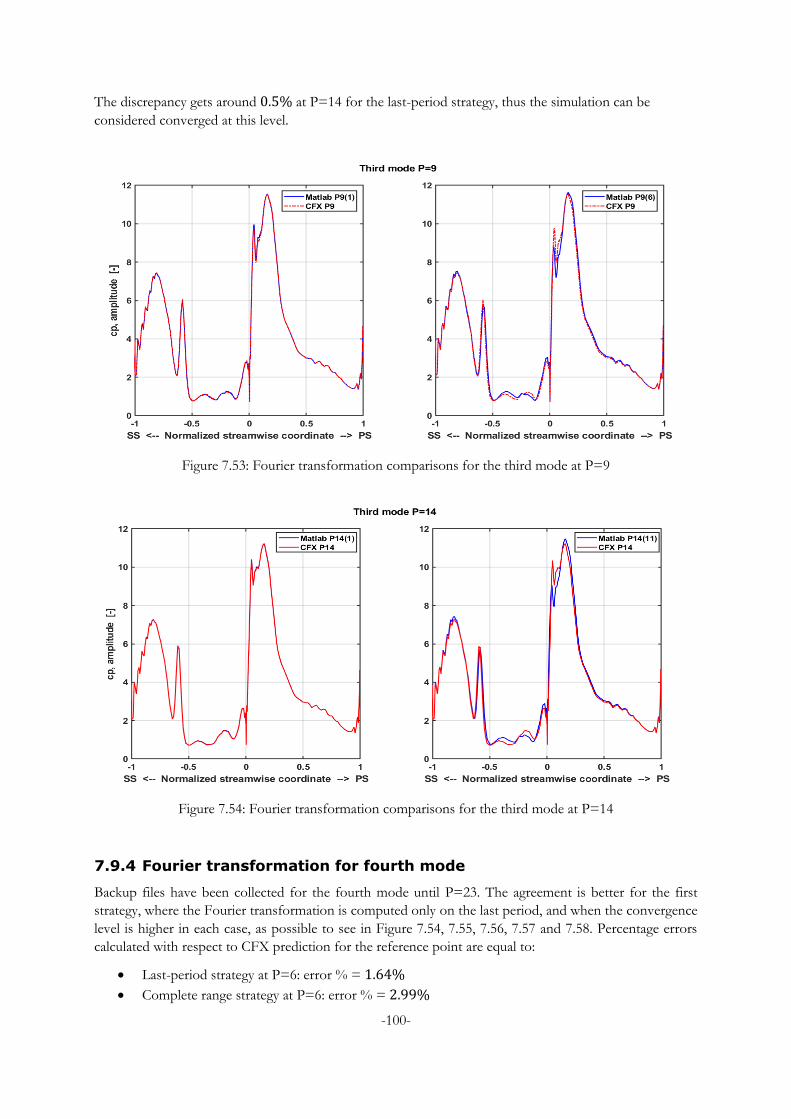
-100-
The discrepancy gets around 0.5% at P=14 for the last-period strategy, thus the simulation can be
considered converged at this level.
Figure 7.53: Fourier transformation comparisons for the third mode at P=9
Figure 7.54: Fourier transformation comparisons for the third mode at P=14
7.9.4 Fourier transformation for fourth mode
Backup files have been collected for the fourth mode until P=23. The agreement is better for the first
strategy, where the Fourier transformation is computed only on the last period, and when the convergence
level is higher in each case, as possible to see in Figure 7.54, 7.55, 7.56, 7.57 and 7.58. Percentage errors
calculated with respect to CFX prediction for the reference point are equal to:
Last-period strategy at P=6: error % = 1.64%
Complete range strategy at P=6: error % = 2.99%
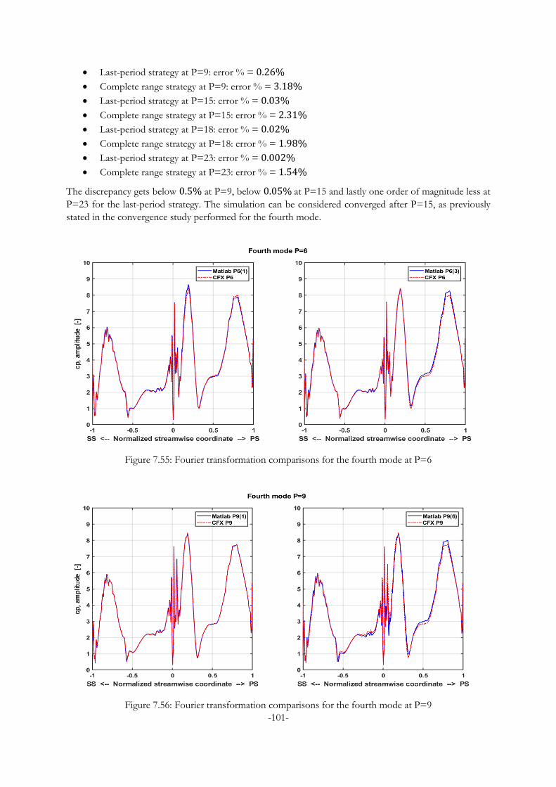
-101-
Last-period strategy at P=9: error % = 0.26%
Complete range strategy at P=9: error % = 3.18%
Last-period strategy at P=15: error % = 0.03%
Complete range strategy at P=15: error % = 2.31%
Last-period strategy at P=18: error % = 0.02%
Complete range strategy at P=18: error % = 1.98%
Last-period strategy at P=23: error % = 0.002%
Complete range strategy at P=23: error % = 1.54%
The discrepancy gets below 0.5% at P=9, below 0.05% at P=15 and lastly one order of magnitude less at
P=23 for the last-period strategy. The simulation can be considered converged after P=15, as previously
stated in the convergence study performed for the fourth mode.
Figure 7.55: Fourier transformation comparisons for the fourth mode at P=6
Figure 7.56: Fourier transformation comparisons for the fourth mode at P=9
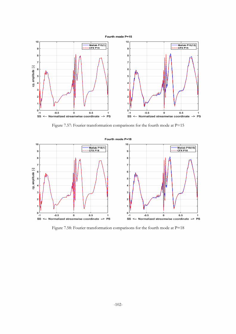
-102-
Figure 7.57: Fourier transformation comparisons for the fourth mode at P=15
Figure 7.58: Fourier transformation comparisons for the fourth mode at P=18
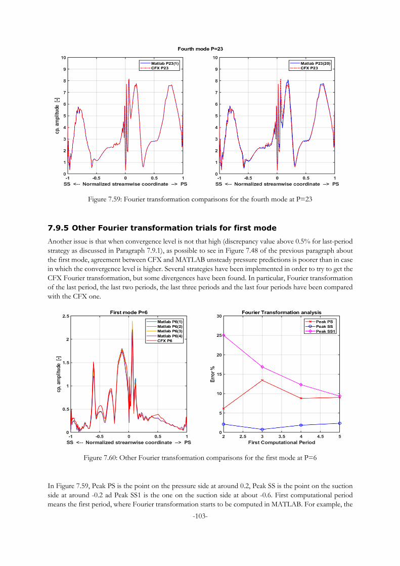
-103-
Figure 7.59: Fourier transformation comparisons for the fourth mode at P=23
7.9.5 Other Fourier transformation trials for first mode
Another issue is that when convergence level is not that high (discrepancy value above 0.5% for last-period
strategy as discussed in Paragraph 7.9.1), as possible to see in Figure 7.48 of the previous paragraph about
the first mode, agreement between CFX and MATLAB unsteady pressure predictions is poorer than in case
in which the convergence level is higher. Several strategies have been implemented in order to try to get the
CFX Fourier transformation, but some divergences have been found. In particular, Fourier transformation
of the last period, the last two periods, the last three periods and the last four periods have been compared
with the CFX one.
Figure 7.60: Other Fourier transformation comparisons for the first mode at P=6
In Figure 7.59, Peak PS is the point on the pressure side at around 0.2, Peak SS is the point on the suction
side at around -0.2 ad Peak SS1 is the one on the suction side at about -0.6. First computational period
means the first period, where Fourier transformation starts to be computed in MATLAB. For example, the
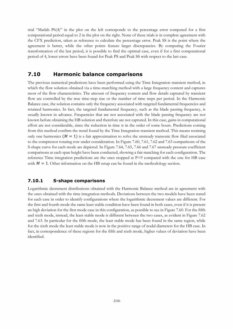
-104-
trial “Matlab P6(4)” in the plot on the left corresponds to the percentage error computed for a first
computational period equal to 2 in the plot on the right. None of these trials is in complete agreement with
the CFX prediction, taken as reference to calculate the percentage error. Peak SS is the point where the
agreement is better, while the other points feature larger discrepancies. By computing the Fourier
transformation of the last period, it is possible to find the optimal case, even if for a first computational
period of 4, lower errors have been found for Peak PS and Peak SS with respect to the last case.
7.10 Harmonic balance comparisons
The previous numerical predictions have been performed using the Time Integration transient method, in
which the flow solution obtained via a time-marching method with a large frequency content and captures
most of the flow characteristics. The amount of frequency content and flow details captured by transient
flow are controlled by the true time-step size or the number of time steps per period. In the Harmonic
Balance case, the solution contains only the frequency associated with targeted fundamental frequencies and
retained harmonics. In fact, the targeted fundamental frequency, such as the blade passing frequency, is
usually known in advance. Frequencies that are not associated with the blade passing frequency are not
known before obtaining the HB solution and therefore are not captured. In this case, gains in computational
effort are not considerable, since the reduction in time is in the order of some hours. Predictions coming
from this method confirm the trend found by the Time Integration transient method. This means retaining
only one harmonics (𝑀 = 1) is a fair approximation to solve the unsteady transonic flow filed associated
to the compressor rotating row under consideration. In Figure 7.60, 7.61, 7.62 and 7.63 comparisons of the
S-shape curve for each mode are depicted. In Figure 7.64, 7.65, 7.66 and 7.67 unsteady pressure coefficient
comparisons at each span height have been conducted, showing a fair matching for each configuration. The
reference Time integration predictions are the ones stopped at P=9 compared with the one for HB case
with 𝑀 = 1. Other information on the HB setup can be found in the methodology section.
7.10.1 S-shape comparisons
Logarithmic decrement distributions obtained with the Harmonic Balance method are in agreement with
the ones obtained with the time integration methods. Deviations between the two models have been stated
for each case in order to identify configurations where the logarithmic decrement values are different. For
the first and fourth mode the same least stable condition have been found in both cases, even if it is present
an high deviation for the first mode case in this configuration, as possible to see in Figure 7.60. For the fifth
and sixth mode, instead, the least stable mode is different between the two cases, as evident in Figure 7.62
and 7.63. In particular for the fifth mode, the least stable mode has been found in the same region, while
for the sixth mode the least stable mode is now in the positive range of nodal diameters for the HB case. In
fact, in correspondence of these regions for the fifth and sixth mode, higher values of deviation have been
identified.
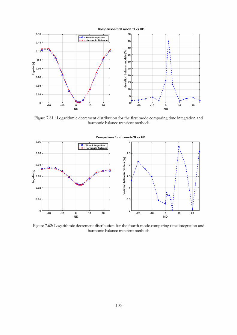
-105-
Figure 7.61 : Logarithmic decrement distribution for the first mode comparing time integration and harmonic balance transient methods
Figure 7.62: Logarithmic decrement distribution for the fourth mode comparing time integration and harmonic balance transient methods
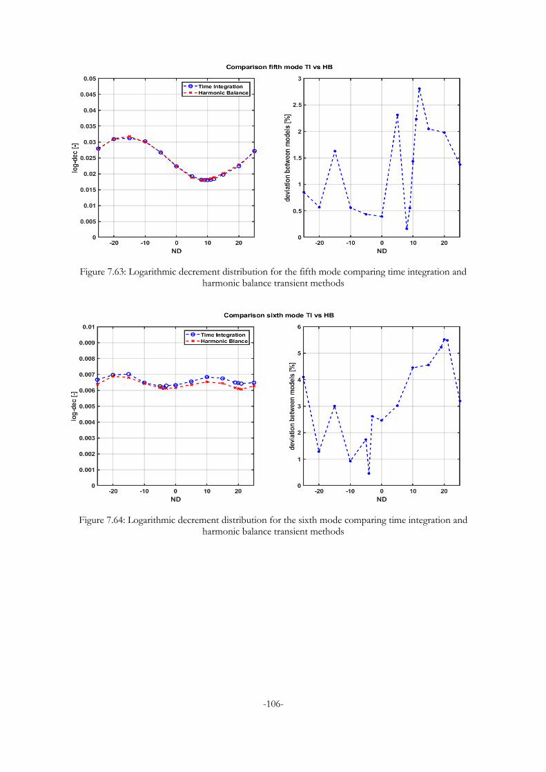
-106-
Figure 7.63: Logarithmic decrement distribution for the fifth mode comparing time integration and harmonic balance transient methods
Figure 7.64: Logarithmic decrement distribution for the sixth mode comparing time integration and harmonic balance transient methods
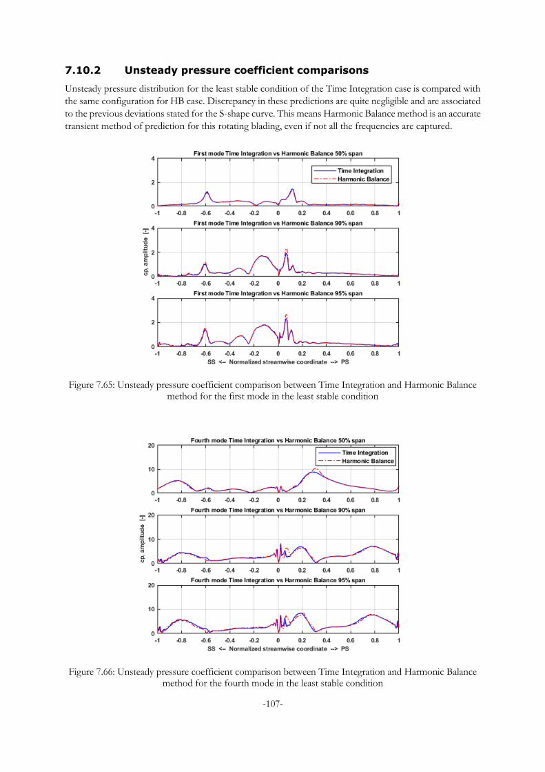
-107-
7.10.2 Unsteady pressure coefficient comparisons
Unsteady pressure distribution for the least stable condition of the Time Integration case is compared with
the same configuration for HB case. Discrepancy in these predictions are quite negligible and are associated
to the previous deviations stated for the S-shape curve. This means Harmonic Balance method is an accurate
transient method of prediction for this rotating blading, even if not all the frequencies are captured.
Figure 7.65: Unsteady pressure coefficient comparison between Time Integration and Harmonic Balance method for the first mode in the least stable condition
Figure 7.66: Unsteady pressure coefficient comparison between Time Integration and Harmonic Balance method for the fourth mode in the least stable condition
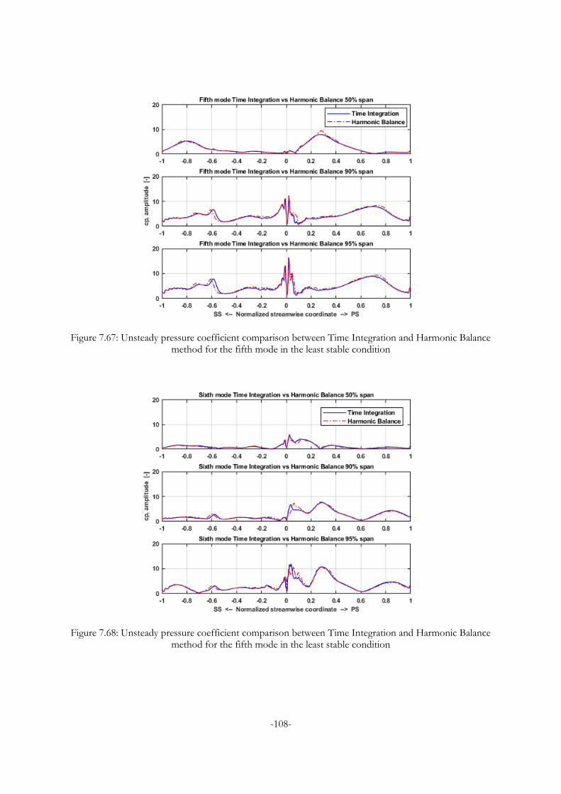
-108-
Figure 7.67: Unsteady pressure coefficient comparison between Time Integration and Harmonic Balance method for the fifth mode in the least stable condition
Figure 7.68: Unsteady pressure coefficient comparison between Time Integration and Harmonic Balance method for the fifth mode in the least stable condition
-109-
8 CONCLUSION AND FUTURE WORK
In this numerical study conducted on the first stage of VINK6 compressor, steady-state blade loading and
Mach number flow field in design condition (design throttle and nominal rotational speed) and aerodynamic
damping for the first six modes have been investigated. The numerical tool chosen for the analysis is ANSYS
CFX, composed by CFX-Pre, which is used for setting the transient method and the numerical parameters,
CFX-Solver and CFD-post, useful for post-processing the solution and getting insights into the quantities
of interest as function of the initial setup. Firstly, steady-state simulations of the whole stage has been
computed. Three different mesh refinements have been used for k-epsilon and SST turbulence model. Only
the rotor blade loading has been taken into account since successive unsteady simulations aims to get
aerodynamic damping of this rotating blade row for different blade deformations. Steady-state blade loading
with k-epsilon model are mesh independent, thus the medium mesh refinement represents the optimum
case in terms of computational effort and accuracy. Steady-state blade loading with SST model predicts a
less sharp shock along the suction side and especially for higher span locations mesh independence is not
completely verified. Therefore, in this case, it is fair to continue investigating the finest mesh in order to try
to understand unsteady phenomena occurring due to this turbulence approach. The blade is more fore-
loaded for higher span heights since the shock at mid-chord occurs at higher streamwise locations. The
Mach flow field shows a bow shock at the leading edge, which propagates until mid-chord of the adjacent
blade. After the shock the flow gets subsonic, while before it is supersonic since the compressor operates
in the transonic regime. Steady-state simulations of the rotor alone have been after conducted in order to
match the blade loading curve of the rotor obtained from the stage simulation. From here on, only medium
mesh with k-epsilon model and fine mesh with SST model have been employed. After getting the same
trend for rotor steady simulation, unsteady investigations have been set up. Two different transient methods
have been used, which are Time Integration and Harmonic Balance method. Logarithmic decrement
distribution computed with the Energy Method has been calculated for the first, fourth, fifth and sixth
mode. The first mode is the only one affected by possible flutter risk as the least stable mode approaches
the stability line. The other modes feature high reduced frequencies, out of the critical range found in
literature, thus the flutter risk is not relevant. The average value and the peak-to-peak amplitude of the S-
shape curves are higher as much as lower natural frequency of the modes is. In fact, the first mode features
the highest average value and peak-to-peak amplitude. Deviation between aerodamping values for the two
blades prescribed by the Fourier transformation method has been stated for each S-shape curve and it is
higher where the logarithmic decrement is lower. For 𝑁𝐷 = 0, deviation values seem accurate for all the
investigated mode. For higher reduced-frequency modes convergence has been tougher to be attained than
for the first mode; simulations of these cases have been extended to P=35 getting Peak-to-Peak and Steady-
Value torque error equal to 0. This means simulations are completely convergent but for the fourth and
fifth mode a discrepancy between aerodamping values of the two blades is still present. The causes of this
mismatch can be related to numerical issue, as the non-reflective boundary conditions at inlet and outlet of
the domain. SST and k-epsilon turbulence model have been compared for the unsteady case; again the SST
model shows a less sharp pressure peak, but the unsteady pressure and local work coefficient distribution
are almost the same as the k-epsilon case for each span location. From here on, only the k-epsilon turbulence
model has been used in unsteady simulations. By simulating only the last stable condition for the second
and third mode and taking only the least stable condition from the S-shape curve for the other analyzed
modes interesting insights can be obtained in terms of unsteady pressure and local work coefficient
distribution. Each mode has its displacement amplitudes and directions, which lead to different pressure
profiles and unstable regions as function of the span and streamwise location. At 95% span all the unsteady
pressure distributions are comparable since the highest displacement has been found in this area; at 50%
span unsteady pressure profiles depend on the specific mode shape. In general higher unsteady pressure
values have been found at higher span location, except for the fourth and fifth mode cases where the specific
direction of these mode shapes lead to higher unsteadiness around mid-span region. The first mode pressure

-110-
profile features lower unsteady pressure values than other modes, however a deeper study has shown the
dependence on the unsteady pressure phase in this case, which can be unfavorable in same configurations
and yield lower pressure values. A deeper study has also be performed for the fourth mode, where
convergence level has been investigated and scaling factor. In particular doubling or halving the scaling
factor, doubled or halved unsteady pressure should be obtained. However, this analysis has shown some
non-linearities since the unsteady pressure distribution are not perfectly consistent. CFX Fourier
transformation has been checked with the one implemented in MATLAB with the Fast Fourier Transform
(FFT) function. From this investigation it can be concluded that when the convergence level is below 0.1%
for Peak-to-Peak and Steady-Value torque error both by computing the Fourier transformation in MATLAB
for the last period the agreement with CFX predictions is almost perfect. The discrepancy values between
the two predictions in a given significant streamwise position have been quantified and convergence level
can be considered acceptable when discrepancy values are below 0.5%. This means CFX predictions are
quite reliable since they make use of converged pressure values. Harmonic balance method has shown the
same trend of S-shape curve, unsteady pressure coefficient and local work coefficient distribution that
means these numerical predictions are robust enough with respect to the numerical setup.
Future works can make use of these predictions to build up the cascade test rig and try to get an agreement
between experimental measurements and numerical values. Unsteady pressure on the blade due to the fluid
flow and aerodamping values have been predicted and validated for a wide range of cases, therefore further
more specific investigations on the same blading can be performed starting from these results.

-111-
Bibliography
[1]Petrie-Repar, P.
Lecture notes, Aeromechanics project course, Kungliga Tekniska Högskolan, Department of Energy Technology (2019)
[2]Jiří Čečrdle
"Whirl Flutter of Turboprop Aircraft Structures", Woodhead Publishing (2015)
[3]Fridh, J., Glodic N.
Lecture notes, Thermal Turbomachinery course, Kungliga Tekniska Högskolan, Department of Energy Technology (2019)
[4]Fasana, A., Marchesiello, S.
"Meccanica delle vibrazioni", CLUT (2006)
[5]Bendiksen, O., Kielb, R.E., Hall, K.C.
''Turbomachinery Aeroelasticity'', Encyclopedia of Aerospace Engineering, John Wiley & Sons, Ltd (2010)
[6]Doi, H.
"Fluid/Structure Coupled Aeroelastic Computations For Transonic Flows in Turbomachinery", a dissertation
submitted to the department of aeronautics and astronautics and the committee on graduate studies of Stanford University in
partial fulfillment of the requirements for the degree of doctor of philosophy (2002)
[7] Biollo,R., Benini, E.
"Recent advances in transonic axial compressor aerodynamics", Prog. Aerosp. Sci. (2013)
[8]Albin, B.
''Transonic flow in turbomachines'', Computerized Educational Platform Heat and Power Technology,
Stockolm/Lausanne (2005)
[9]Rampado, M.
"Analisi numerica dell’interazione fluido-strutturale in una turbina di bassa pressione", Tesi di laurea magistrale,
Università Degli Studi di Padova, Dipartimento di Ingegneria Industriale DII (2015)
[10] Verdon, J. M.
''Linearized Unsteady Aerodynamic Theory'', AGARD Manual on Aeroelasticity in Axial-Flow Turbomachines,
Vol. 1, Unsteady Turbomachinery Aerodynamics, Chapter 2 (1987)
[11]Zhao, F., Nipkau, J., Vahdati, M.
''Influence of acoustic reflection on flutter stability of an embedded blade row'', Mechanical Engineering
Department, Imperial College London, London, UK (2015)
[12]Vogt, D.M.
''Experimental Investigations of Three-Dimensional Mechanisms in Low-Pressure Turbine Flutter'', Doctoral
Thesis, Kungliga Tekniska Högskolan, Department of Energy Technology, Stockholm (2005)
[13] Panovsky, J., Kielb, R. E.
''A Design Method to Prevent Low Pressure Turbine Blade Flutter'', Journal of Engineering for Gas Turbines and
Power, Vol. 122, pp. 89-98 (2000)
-112-
[14]Chernysheva, O.V., Fransson, T.H., Kielb, R.E., Barter, J.
''Influence of a Vibration Amplitude Distribution on the Aerodynamic Stability of a Low-
Pressure Turbine Sectored Vane'', proceedings 10th International Symposium on Aerodynamics, Aeroacoustics and
Aeroelasticity of Turbomachines (ISUAAAT), Durham, North Carolina, USA (2003)
[15]Crawley, E. F.
''Aeroelastic Formulation for Tuned and Mistuned Rotors'', AGARD Manual on Aeroelasticity in Axial-Flow
Turbomachines, Vol.2, Structural Dynamics and Aeroelasticity, Chapter 19 (1988)
[16]Fransson, T.H., Et al
''Aeroelasticity in Turbomachines comparison of Theoretical and Experimental Cascade Results'', EPFL,
Lausanne (1986)
[17] Torsten, H., Fransson, T.H.
''Aeroelasticity in Axial-Flow Turbomachines'', Book 1 and Book 2
[18]Stasolla, V., Carillo Segura, S., Mohan, A., Bakhshandeh, M.
Minor project technical report, Aeromech project course, Kungliga Tekniska Högskolan, Department of Energy
Technology (2019)
[19]Nowinski, M., Panovsky, J.
''Flutter Mechanisms in Low Pressure Turbine Blades'', J. of Engineering for Gas Turbines and Power, Vol. 122,
2000, pp. 82-88 (2000)
[20]Glodic, N.
''Sensitivity of Aeroelastic Properties of an Oscillating LPT Cascade'', Licentiate Thesis, Kungliga Tekniska
Högskolan, Department of Energy Technology, Stockholm (2013)
[21]Lejon, M., Grönstedt, T., Glodic, N., Petrie-Repar, P.,Genrup, M., Mann, A.
''Multidisciplinary design of a three stage high speed booster'', Turbine Technical Conference and Exposition,
ASME, Charlotte, USA (2013)
[22]Fröhler, B.
"Aeroelastic Investigation of the 1st Stage VINK Compressor", Technical report, Thrust Internship, Kungliga
Tekniska Högskolan, Department of Energy Technology (2017)
[23]ANSYS CFX 19.2
"ANSYS CFX 19.2 Documentation", ANSYS (2019)
[24]Raw M.
"A new Control-Volume based Finite Element Procedure for the Numerical Solution of the Fluid Flow and
Scalar Transport Equations", Ph.D.Thesis, University of Waterloo, Canada (1985)
[25]Barth T. J., Jesperson D.C.
"The Design and Application of Upwind Schemes on Unstructured Meshes", AIAA Paper 89-0366 (1989)
[26]Rhie C. M., Chow W. L.
"Numerical Study of the Turbulent Flow past an Airfoil with Trailing Edge Separation", AIAA Journal, 21,
1525-1532 (1983)
-113-
[27]Hutchinson, B. R., Raithby, G. D.
"A Multigrid Method based on the Additive Correction Strategy", Numerical Heat Transfer, 19, 511-530 (1986)
[28]Raw, M.
"Robustness of Coupled Algebraic Multigrid for Navier-Stokes Equations", AIAA Paper-960297, 34th
AIAA Aerospace Science Meeting, Reno (1996)
[29]Versteeg, H.K., Malalaseker, W.
''An Introduction to Computational Fluid Dynamics'', Pearson Education Limited 1995, 2nd edition (2007)
[30]Menter, F. R.
"Two-equation Eddy-viscosity Turbulence Models for Engineering Applications", AIAA Journal, 32(8),
1598 – 1605 (1994)
[31]Elder, R., Woods, I., Patil, S., Holmes W., Steed, R., Hutchinson, B.
''Investigation of efficient cfd methods for the prediction of blade damping'', Turbine Technical Conference and
Exposition, ASME, San Antonio, Texas, USA (2013)
[32]Hall, K.C, Jeffrey, P. T., Clark, W.S.
''Computation of Unsteady Nonlinear Flow in Cascades Using a Harmonic Balance Technique'', Duke
University, Durham, North Carolina (2002)
[33]Cornelius, C., Biesinger, T., Galpin, P., Braune, A.
" Experimental and Computational Analysis of a Multistage Axial Compressor Including Stall Prediction by
Steady and Transient CFD Methods ", J. Turbomach., vol. 136, no. 6 (2013)
[34] Zeeshan, S.
"Feasibility of Using Morphing Inlet Guide Vanes for Improved Aerodynamics Performance and Reduced
Forcing", Master Thesis Report, Kungliga Tekniska Högskolan, Department of Energy Technology, Stockholm (2017)
[35]Cumpsty, N.A.
"Compressor Aerodynamics", Longman Group UK ltd (1989)


![Influence of Transonic Flutter on the Conceptual Design of ......V? = Wing-perpendicularvelocity a = Acceleration b = Wingspan ... subsonic, and supersonic flow. Theodorsen [10],](https://img.pdfslide.us/doc/110x75/5e88fb902e59b70b946d6699/influence-of-transonic-flutter-on-the-conceptual-design-of-v-wing-perpendicularvelocity.jpg)