Numerical Analysis Notes for Math 575Amath.arizona.edu/~faris/Num.pdf · Numerical Analysis Notes for Math 575A William G. Faris Program in Applied Mathematics University of Arizona

Numerical Analysis

Notes for Math 575A

William G. FarisProgram in Applied Mathematics

University of Arizona

Fall 1992

Contents

1 Nonlinear equations 51.1 Introduction . . . . . . . . . . . . . . . . . . . . . . . . . . . 51.2 Bisection . . . . . . . . . . . . . . . . . . . . . . . . . . . . 51.3 Iteration . . . . . . . . . . . . . . . . . . . . . . . . . . . . . 9

1.3.1 First order convergence . . . . . . . . . . . . . . . . 91.3.2 Second order convergence . . . . . . . . . . . . . . . 11

1.4 Some C notations . . . . . . . . . . . . . . . . . . . . . . . . 121.4.1 Introduction . . . . . . . . . . . . . . . . . . . . . . 121.4.2 Types . . . . . . . . . . . . . . . . . . . . . . . . . . 131.4.3 Declarations . . . . . . . . . . . . . . . . . . . . . . . 141.4.4 Expressions . . . . . . . . . . . . . . . . . . . . . . . 141.4.5 Statements . . . . . . . . . . . . . . . . . . . . . . . 161.4.6 Function definitions . . . . . . . . . . . . . . . . . . 17

2 Linear Systems 192.1 Shears . . . . . . . . . . . . . . . . . . . . . . . . . . . . . . 192.2 Reflections . . . . . . . . . . . . . . . . . . . . . . . . . . . . 242.3 Vectors and matrices in C . . . . . . . . . . . . . . . . . . . 27

2.3.1 Pointers in C . . . . . . . . . . . . . . . . . . . . . . 272.3.2 Pointer Expressions . . . . . . . . . . . . . . . . . . 28

3 Eigenvalues 313.1 Introduction . . . . . . . . . . . . . . . . . . . . . . . . . . . 313.2 Similarity . . . . . . . . . . . . . . . . . . . . . . . . . . . . 313.3 Orthogonal similarity . . . . . . . . . . . . . . . . . . . . . . 34

3.3.1 Symmetric matrices . . . . . . . . . . . . . . . . . . 343.3.2 Singular values . . . . . . . . . . . . . . . . . . . . . 343.3.3 The Schur decomposition . . . . . . . . . . . . . . . 35

3.4 Vector and matrix norms . . . . . . . . . . . . . . . . . . . 373.4.1 Vector norms . . . . . . . . . . . . . . . . . . . . . . 37

1

2 CONTENTS

3.4.2 Associated matrix norms . . . . . . . . . . . . . . . 373.4.3 Singular value norms . . . . . . . . . . . . . . . . . . 383.4.4 Eigenvalues and norms . . . . . . . . . . . . . . . . . 393.4.5 Condition number . . . . . . . . . . . . . . . . . . . 39

3.5 Stability . . . . . . . . . . . . . . . . . . . . . . . . . . . . . 403.5.1 Inverses . . . . . . . . . . . . . . . . . . . . . . . . . 403.5.2 Iteration . . . . . . . . . . . . . . . . . . . . . . . . . 403.5.3 Eigenvalue location . . . . . . . . . . . . . . . . . . . 41

3.6 Power method . . . . . . . . . . . . . . . . . . . . . . . . . . 433.7 Inverse power method . . . . . . . . . . . . . . . . . . . . . 443.8 Power method for subspaces . . . . . . . . . . . . . . . . . . 443.9 QR method . . . . . . . . . . . . . . . . . . . . . . . . . . . 463.10 Finding eigenvalues . . . . . . . . . . . . . . . . . . . . . . . 47

4 Nonlinear systems 494.1 Introduction . . . . . . . . . . . . . . . . . . . . . . . . . . . 494.2 Degree . . . . . . . . . . . . . . . . . . . . . . . . . . . . . . 51

4.2.1 Brouwer fixed point theorem . . . . . . . . . . . . . 524.3 Iteration . . . . . . . . . . . . . . . . . . . . . . . . . . . . . 52

4.3.1 First order convergence . . . . . . . . . . . . . . . . 524.3.2 Second order convergence . . . . . . . . . . . . . . . 54

4.4 Power series . . . . . . . . . . . . . . . . . . . . . . . . . . . 564.5 The spectral radius . . . . . . . . . . . . . . . . . . . . . . . 564.6 Linear algebra review . . . . . . . . . . . . . . . . . . . . . 574.7 Error analysis . . . . . . . . . . . . . . . . . . . . . . . . . . 59

4.7.1 Approximation error and roundoff error . . . . . . . 594.7.2 Amplification of absolute error . . . . . . . . . . . . 594.7.3 Amplification of relative error . . . . . . . . . . . . . 61

4.8 Numerical differentiation . . . . . . . . . . . . . . . . . . . . 63

5 Ordinary Differential Equations 655.1 Introduction . . . . . . . . . . . . . . . . . . . . . . . . . . . 655.2 Numerical methods for scalar equations . . . . . . . . . . . 655.3 Theory of scalar equations . . . . . . . . . . . . . . . . . . . 67

5.3.1 Linear equations . . . . . . . . . . . . . . . . . . . . 675.3.2 Autonomous equations . . . . . . . . . . . . . . . . . 675.3.3 Existence . . . . . . . . . . . . . . . . . . . . . . . . 685.3.4 Uniqueness . . . . . . . . . . . . . . . . . . . . . . . 695.3.5 Forced oscillations . . . . . . . . . . . . . . . . . . . 70

5.4 Theory of numerical methods . . . . . . . . . . . . . . . . . 715.4.1 Fixed time, small step size . . . . . . . . . . . . . . . 715.4.2 Fixed step size, long time . . . . . . . . . . . . . . . 73

CONTENTS 3

5.5 Systems . . . . . . . . . . . . . . . . . . . . . . . . . . . . . 775.5.1 Introduction . . . . . . . . . . . . . . . . . . . . . . 775.5.2 Linear constant coefficient equations . . . . . . . . . 775.5.3 Stiff systems . . . . . . . . . . . . . . . . . . . . . . 815.5.4 Autonomous Systems . . . . . . . . . . . . . . . . . 825.5.5 Limit cycles . . . . . . . . . . . . . . . . . . . . . . . 84

6 Fourier transforms 876.1 Groups . . . . . . . . . . . . . . . . . . . . . . . . . . . . . . 876.2 Integers mod N . . . . . . . . . . . . . . . . . . . . . . . . . 876.3 The circle . . . . . . . . . . . . . . . . . . . . . . . . . . . . 896.4 The integers . . . . . . . . . . . . . . . . . . . . . . . . . . . 896.5 The reals . . . . . . . . . . . . . . . . . . . . . . . . . . . . 896.6 Translation Invariant Operators . . . . . . . . . . . . . . . . 906.7 Subgroups . . . . . . . . . . . . . . . . . . . . . . . . . . . . 926.8 The sampling theorem . . . . . . . . . . . . . . . . . . . . . 946.9 FFT . . . . . . . . . . . . . . . . . . . . . . . . . . . . . . . 95æ

4 CONTENTS

Chapter 1

Nonlinear equations

1.1 Introduction

This chapter deals with solving equations of the form f(x) = 0, where f isa continuous function.

The usual way in which we apply the notion of continuity is throughsequences. If g is a continuous function, and cn is a sequence such thatcn → c as n→∞, then g(cn)→ g(c) as n→∞.

Here is some terminology that we shall use. A number x is said to bepositive if x ≥ 0. It is strictly positive if x > 0. (Thus we avoid the mind-numbing term “non-negative.”) A sequence an is said to be increasing ifan ≤ an+1 for all n. It is said to be strictly increasing if an < an+1 forall n. There is a similar definition for what it means for a function to beincreasing or strictly increasing. (This avoids the clumsy locution “non-decreasing.”)

Assume that a sequence an is increasing and bounded above by somec < ∞, so that an ≤ c for all n. Then it is always true that there is ana ≤ c such that an → a as n→∞.

1.2 Bisection

The bisection method is a simple and useful way of solving equations. It isa constructive implementation of the proof of the following theorem. Thisresult is a form of the intermediate value theorem.

Theorem 1.2.1 Let g be a continuous real function on a closed interval[a, b] such that g(a) ≤ 0 and g(b) ≥ 0. Then there is a number r in the

5

6 CHAPTER 1. NONLINEAR EQUATIONS

interval with g(r) = 0.

Proof: Construct a sequence of intervals by the following procedure.Take an interval [a, b] on which g changes sign, say with g(a) ≤ 0 andg(b) ≥ 0. Let m = (a + b)/2 be the midpoint of the interval. If g(m) ≥ 0,then replace [a, b] by [a,m]. Otherwise, replace [a, b] by [m, b]. In eithercase we obtain an interval of half the length on which g changes sign.

The sequence of left-hand points an of these intervals is an increasingsequence bounded above by the original right-hand end point. Thereforethis sequence converges as n → ∞. Similarly, the sequence of right-handpoints bn is a decreasing sequence bounded below by the original left-handend point. Therefore it also converges. Since the length bn − an goes tozero as n→∞, it follows that the two sequences have the same limit r.

Since g(an) ≤ 0 for all n, we have that g(r) ≤ 0. Similarly, sinceg(bn) ≥ 0 for all n, we also have that g(r) ≥ 0. Hence g(r) = 0. 2

Note that if a and b are the original endpoints, then after n steps oneis guaranteed to have an interval of length (b− a)/2n that contains a root.

In the computer implementation the inputs to the computation involvegiving the endpoints a and b and the function g. One can only do a certainnumber of steps of the implementation. There are several ways of accom-plishing this. One can give the computer a tolerance and stop when thethe length of the interval does not exceed this value. Alternatively, onecan give the computer a fixed number of steps nsteps. The output is thesequence of a and b values describing the bisected intervals.

void bisect(real tolerance, real a, real b, real (*g)(real) )

{

real m ;

while( b - a > tolerance )

{

m = (a+b) / 2 ;

if( g(a) * g(m) <= 0.0 )

b = m ;

else

a = m ;

display(a, b) ;

}

}

The construction here is the while loop, which is perhaps the mostfundamental technique in programming.

Here is an alternative version in which the iterations are controlled bya counter n.

1.2. BISECTION 7

void bisect(int nsteps, real a, real b, real (*g)(real) )

{

int n ;

real m ;

n = 0 ;

while( n < nsteps )

{

m = (a+b) / 2 ;

if( g(a) * g(m) <= 0.0 )

b = m ;

else

a = m ;

n = n + 1 ;

display(n, a, b) ;

}

}

Algorithms such as this are actual computer code in the programminglanguage C. It should be rather easy to read even without a knowledge ofC. The key word void indicates that the bisect function is a procedure andnot a function that returns a meaningful value. The parameter declarationreal (*g)(real) indicates that g is a variable that can point to functionsthat have been defined (real functions of real arguments). When readingthe text of a function such as bisect, it is useful to read the sign = as“becomes.”

To make a complete program, one must put this in a program that callsthis procedure.

/* bisection */

#include <stdio.h>

#include <math.h>

typedef double real;

void bisect(int, real, real, real (*)(real));

real quadratic(real) ;

void fetch(int *, real *, real *);

void display(int, real, real) ;

int main()

{

int nsteps;


real a, b;

real (*f)(real);

f = quadratic;

fetch(nsteps, a, b);

display(nsteps,a,b);

bisect(nsteps,a,b,f);

return 0;

}

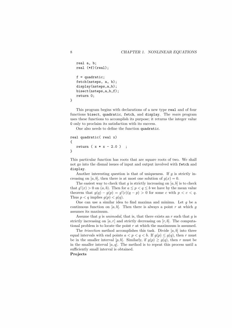
This program begins with declarations of a new type real and of fourfunctions bisect, quadratic, fetch, and display. The main programuses these functions to accomplish its purpose; it returns the integer value0 only to proclaim its satisfaction with its success.

One also needs to define the function quadratic.

real quadratic( real x)

{

return ( x * x - 2.0 ) ;

}

This particular function has roots that are square roots of two. We shallnot go into the dismal issues of input and output involved with fetch anddisplay.

Another interesting question is that of uniqueness. If g is strictly in-creasing on [a, b], then there is at most one solution of g(x) = 0.

The easiest way to check that g is strictly increasing on [a, b] is to checkthat g′(x) > 0 on (a, b). Then for a ≤ p < q ≤ b we have by the mean valuetheorem that g(q) − g(p) = g′(c)(q − p) > 0 for some c with p < c < q.Thus p < q implies g(p) < g(q).

One can use a similar idea to find maxima and minima. Let g be acontinuous function on [a, b]. Then there is always a point r at which gassumes its maximum.

Assume that g is unimodal, that is, that there exists an r such that g isstrictly increasing on [a, r] and strictly decreasing on [r, b]. The computa-tional problem is to locate the point r at which the maximuum is assumed.

The trisection method accomplishes this task. Divide [a, b] into threeequal intervals with end points a < p < q < b. If g(p) ≤ g(q), then r mustbe in the smaller interval [p, b]. Similarly, if g(p) ≥ g(q), then r must bein the smaller interval [a, q]. The method is to repeat this process until asufficiently small interval is obtained.

Projects

1.3. ITERATION 9

1. Write a bisection program to find the square roots of two. Find them.

2. Use the program to solve sinx = x2 for x > 0.

3. Use the program to solve tanx = x with π/2 < x < 3π/2.

4. Write a trisection program to find maxima. Use it to find the mini-mum of h(x) = x3/3 + cosx for x ≥ 0.

Problems

1. Show that sinx = x2 has a solution with x > 0. Be explicit aboutthe theorems that you use.

2. Show that sinx = x2 has at most one solution with x > 0.

3. Show that tanx = x has a solution with π/2 < x < 3π/2.

4. Show that x5 − x+ 1/4 = 0 has has at least two solutions between 0and 1.

5. Show that x5 − x+ 1/4 = 0 has has at most two solutions between 0and 1.

6. Prove a stronger form of the intermediate value theorem: if g is con-tinuous on [a, b], then g assumes every value in [g(a), g(b)].

7. How many decimal places of accuracy does one gain at each bisection?

8. How many decimal places are obtained at each trisection?

1.3 Iteration

1.3.1 First order convergence

Recall the intermediate value theorem: If f is a continuous function on theinterval [a, b] and f(a) ≤ 0 and f(b) ≥ 0, then there is a solution of f(x) = 0in this interval.

This has an easy consequence: the fixed point theorem. If g is a contin-uous function on [a, b] and g(a) ≥ a and g(b) ≤ b, then there is a solutionof g(x) = x in the interval.

Another approach to numerical root-finding is iteration. Assume thatg is a continuous function. We seek a fixed point r with g(r) = r. We canattempt to find it by starting with an x0 and forming a sequence of iteratesusing xn+1 = g(xn).


Theorem 1.3.1 Let g be continuous and let xn a sequence such that xn+1 =g(xn). Then if xn → r as n→∞, then g(r) = r.

This theorem shows that we need a way of getting sequences to converge.One such method is to use increasing or decreasing sequences.

Theorem 1.3.2 Let g be a continuous function on [r, b] such that g(x) ≤ xfor all x in the interval. Let g(r) = r and assume that g′(x) ≥ 0 forr < x < b. Start with x0 in the interval. Then the iterates defined byxn+1 = g(xn) converge to a fixed point.

Proof: By the mean value theorem, for each x in the interval there isa c with g(x)− r = g(x)− g(r) = g′(c)(x− r). It follows that r ≤ g(x) ≤ xfor r ≤ x ≤ b. In other words, the iterations decrease and are boundedbelow by r. 2

Another approach is to have a bound on the derivative.

Theorem 1.3.3 Assume that g is continuous on [a, b] and that g(a) ≥ aand g(b) ≤ b. Assume also that |g′(x)| ≤ K < 1 for all x in the interval.Let x0 be in the interval and iterate using xn+1 = g(xn). Then the iteratesconverge to a fixed point. Furthermore, this fixed point is unique.

Proof: Let r be a fixed point in the interval. By the mean valuetheorem, for each x there is a c with g(x)− r = g(x)− g(r) = g′(c)(x− r),and so |g(x)− r| = |g′(c)||x− r| ≤ K|x− r|. In other words each iterationreplacing x by g(x) brings us closer to r. 2

We say that r is a stable fixed point if |g′(r)| < 1. We expect convergencewhen the iterations are started near a stable fixed point.

If we want to use this to solve f(x) = 0, we can try to take g(x) =x − kf(x) for some suitable k. If k is chosen so that g′(x) = 1 − kf ′(x) issmall for x near r, then there should be a good chance of convergence.

It is not difficult to program fixed point iteration. Here is a version thatdisplays all the iterates.

void iterate(int nsteps, real x, real (*g)(real) )

{

n = 0 ;

while( n < nsteps)

{

x = g(x) ;

n = n + 1 ;

display(n, x) ;

}

}

1.3. ITERATION 11

1.3.2 Second order convergence

Since the speed of convergence in iteration with g is controlled by g′(r), itfollows that the situation when g′(r) = 0 is going to have special properties.

It is possible to arrange that this happens! Say that one wants to solvef(x) = 0. Newton’s method is to take g(x) = x − f(x)/f ′(x). It is easy tocheck that f(r) = 0 and f ′(r) 6= 0 imply that g′(r) = 0.

Newton’s method is not guaranteed to be good if one begins far fromthe starting point. The damped Newton method is more conservative. Onedefines g(x) as follows. Let m = f(x)/f ′(x) and let y = x − m. While|f(y)| > |f(x)| replace m by m/2 and let y = x−m. Let g(x) be the finalvalue of y.Projects

1. Implement Newton’s method as a special case of the fixed point iter-ations. Use this to find the largest root of sinx − x2 = 0. Describewhat happens if you start the iteration with .46.

2. Implement the damped Newton’s method. Use this to find the largestroot of sinx−x2 = 0. Describe what happens if you start the iterationwith .46.

3. Find all roots of 2 sinx − x = 0 numericallly. Use some version ofNewton’s method.

Problems

1. Let g(x) = (2/3)x + (7/3)(1/x2). Show that for every initial pointx0 above the fixed point the iterations converge to the fixed point.What happens for initial points x0 > 0 below the fixed point?

2. Assume that x ≤ g(x) and g′(x) ≥ 0 for a ≤ x ≤ r. Show thatit follows that x ≤ g(x) ≤ r for a ≤ x ≤ r and that the iterationsincrease to the root.

3. Prove the fixed point theorem from the intermediate value theorem.

4. In fixed point iteration with a g having continuous derivative andstable fixed point r, find the limit of (xn+1−r)/(xn−r). Assume theiterations converge.

5. Perhaps one would prefer something that one could compute numer-ically. Find the limit of (xn+1 − xn)/(xn − xn−1) as n→∞.

6. How many decimal places does one gain at each iteration?


7. In fixed point iteration with a g having derivative g′(r) = 0 andcontinuous second derivative, find the limit of (xn+1 − r)/(xn − r)2.

8. Describe what this does to the decimal place accuracy at each itera-tion.

9. Calculate g′(x) in Newton’s method.

10. Show that in Newton’s method f(r) = 0 with f ′(r) 6= 0 impliesg′(r) = 0.

11. Calculate g′′(x) in Newton’s method.

12. Consider Newton’s method for x3−7 = 0. Find the basin of attractionof the positive root. Be sure to find the entire basin and prove thatyour answer is correct. (The basin of attraction of a fixed point ofan interation function g is the set of all initial points such that fixedpoint iteration starting with that initial point converges to the fixedpoint.)

13. Consider Newton’s method to find the largest root of sinx− x2 = 0.What is the basin of attraction of this root? Give a mathematicalargument that your result is correct.

14. Show that in Newton’s method starting near the root one has eitherincrease to the the root from the left or decrease to the root fromthe right. (Assume that f ′(x) and f ′′(x) are non-zero near the root.)What determines which case holds?

15. Assume that |xn+1 − r| ≤ K|xn − r|2 for all n ≥ 0. Find a conditionon x0 that guarantees that xn → r as n→∞.

16. Is the iteration function in the damped Newton’s method well-defined?Or could the halving of the steps go on forever?

1.4 Some C notations

1.4.1 Introduction

This is an exposition of a fragment of C sufficient to express numericalalgorithms involving only scalars. Data in C comes in various types. Herewe consider arithmetic types and function types.

A C program consists of declarations and function definitions. The dec-larations reserve variables of various types. A function definition describeshow to go from input values to an output value, all of specified types. It

1.4. SOME C NOTATIONS 13

may also define a procedure by having the side effect of changing the valuesof variables.

The working part of a function definition is formed of statements, whichare commands to perform some action, usually changing the values of vari-ables. The calculations are performed by evaluating expressions writtenin terms of constants, variables, and functions to obtain values of varioustypes.

1.4.2 Types

Arithmetic

Now we go to the notation used to write a C program. The basic typesinclude arithmetic types such as:

char

int

float

double

These represent character, integer, floating point, and double precisionfloating point values.

There is also a void type that has no values.A variable of a certain type associates to each machine state a value of

this type. In a computer implementation a variable is realized by a locationin computer memory large enough to hold a value of the appropriate type.

Example: One might declare n to be an integer variable and x to be afloat variable. In one machine state n might have the value 77 and x mighthave the value 3.41.

Function

Another kind of data object is a function. The type of a function dependson the types of the arguments and on the type of the value. The type of thevalue is written first, followed by a list of types of the arguments enclosedin parentheses.

Example: float (int) is the type of a function of an integer argumentreturning float. There might be a function convert of this type defined inthe program.

Example: float ( float (*)(float), float, int) is the type of afunction of three arguments of types float (*)(float), float, and int

returning float. The function iterate defined below is of this type.A function is a constant object given by a function definition. A function

is realized by the code in computer memory that defines the function.


Pointer to function

There are no variable functions, but there can be variables of type pointerto function. The values of such a variable indicate which of the functiondefinitions is to be used.

Example: float (*)(int) is the type of a pointer to a function fromint to float. There could be a variable f of this type. In some machinestate it could point to the function convert.

The computer implementation of pointer to function values is as ad-dresses of memory locations where the functions are stored.

A function is difficult to manipulate directly. Therefore in a C expressionthe value of a function is not the actual function, but the pointer associatedwith the function. This process is known as pointer conversion.

Example: It is legal to make the assignment f = convert.

1.4.3 Declarations

A declaration is a specification of variables or functions and of their types.

A declaration consists of a value type and a list of declarators and isterminated by a semicolon. These declarators associate identifiers with thecorresponding types.

Example: float x, y ; declares the variables x and y to be of typefloat.

Example: float (*g)(float) ; declares g as a pointer to functionfrom float to float.

Example: float iterate( float (*)(float), float, int) ; de-clares a function iterate of three arguments of types float (*)(float),float, and int returning float.

1.4.4 Expressions

Variables

An expression of a certain type associates to each machine state a value ofthis type.

Primary expressions are the expressions that have the highest prece-dence. Constants and variables are primary expressions. An arbitraryexpression can be converted to a primary expression by enclosing it inparentheses.

Usually the value of the variable is the data contained in the variable.However the value of a function is the pointer that corresponds to thefunction.


Example: After the declaration float x, y ; and subsequent assign-ments the variables x and y may have values which are float.

Example: After the declaration float (*g)(float) ; and subsequentassignments the variable g may have a pointer to function on float returninga float value.

Example: After the declaration float iterate( float (*)(float),

float, int) ; and a function definition the function iterate is defined.Its value is the pointer value that corresponds to the function. Thus if his a variable which can point to such a function, then the assignment h =

iterate ; is legal.

Function calls

A function call is an expression formed from a pointer to function expressionand an argument list of expressions. Its value is obtained by finding thepointer value, evaluating the arguments and copying their values, and usingthe function corresponding to the pointer value to calculate the result.

Example: Assume that g is a function pointer that has a pointer tosome function as its value. Then this function uses the value of x to obtaina value for the function call g(x).

Example: The function iterate is defined with the heading iterate(

float (*g)(float), float x, float n ). A function call iterate(square,z, 3) uses the value of iterate, which is a function pointer, and the val-ues of square, x, and 3, which are function pointer, float, and integer. Thevalues of the arguments square, z, and 3 are copied to the parameters g,x, and n. The computation described in the function definition is carriedout, and a float is returned as the value of the function call.

Casts

A data type may be changed by a cast operator. This is indicated byenclosing the type name in parentheses.

Example: 7 / 2 evaluates to 3 while (float)7 / 2 evaluates to 3.5.

Arithmetic and logic

There are a number of ways of forming new expressions from old.The unary operators + and - and the negation ! can form new expres-

sions.Multiplicative expressions are formed by the binary operators *, / and

%. The last represents the remainder in integer division.Additive expressions are formed by the binary operators + and -.


Relational expressions are formed by the inequalities < and <= and >

and >=.Equality expressions are formed by the equality and negated equality ==

and !==.Logical AND expression are formed by &&.Logical OR expression are formed by ||.

Assignments

Another kind of expression is the assignment expression. This is of theform variable = expression. It takes the expression on the right, evaluatesit, and assigns the value to the variable on the left (and to the assignmentexpression). This changes the machine state.

An assignment is is read variable “becomes” expression.Warning: This should be distinguished from an equality expression of the

form expression == expression. This is read expression “equals” expression.Example: i = 0

Example: i = i + 1

Example: x = g(x)

Example: h = iterate, where h is a function pointer variable anditerate is a function constant.

1.4.5 Statements

Expression statements

A statement is a command to perform some action changing the machinestate.

Among the most important are statements formed from expressions(such as assignment expressions) of the form expression ;

Example: i = 0 ;

Example: i = i + 1 ;

Example: x = g(x) ;

Example: h = iterate ;, where h is a function pointer variable anditerate is a function constant.

In the compound statement part of a function definition the statementreturn expression ; stops execution of the function and returns the valueof the expression.

Control statements

There are several ways of building up new statements from old ones. Themost important are the following.


A compound statement is of the form:{ declaration-list statement-list }An if-else statement is of the form:if ( expression ) statement else statementA while statement is of the form:while ( expression ) statementThe following pattern of statements often occurs:expr1 ; while ( expr2 ) { statement expr 3; }Abbreviation: The above pattern is abbreviated by the for statement

of the form:for( expr1 ; expr2 ; expr3 ) statement

1.4.6 Function definitions

A function definition begins with a heading that indicates the type of theoutput, the name of the function, and a parenthesized parameter list. Eachelement of the parameter list is a specification that identifies a parameterof a certain type. The body of a function is a single compound statement.

Example: The definition of square as the squaring function of typefunction of float returning float is

float square( float y )

{

return y*y ;

}

The definition of iterate (with parameters g, x, n of types pointer tofunction of float returning float, float, and integer) returning float is

float iterate( float (*g)(float), float x, float n )

{

int i ;

i = 0 ;

while ( i < n ) do

{

x = g(x) ;

i = i + 1 ;

}

return x ;

}

Example: Consider the main program


main()

{

float z, w ;

z = 2.0 ;

w = iterate(square, z, 3) ;

}

The function call iterate(square, z, 3) has argument expressionswhich are a function square, a float z, and an integer 3. These argumentsare evaluated and the values are copied to the parameters g, x, and n,which are pointer to function, float, and integer objects. In the course ofevaluation the parameter x changes its value, but z does not change itsvalue of 2.0. The value returned by iterate(square,z,3) is 256.0. Theultimate result of the program is to assign 2.0 to z and 256.0 to w.

Chapter 2

Linear Systems

This chapter is about solving systems of linear equations. This is an al-gebraic problem, and it provides a good place in which to explore matrixtheory.

2.1 Shears

In this section we make a few remarks about the geometric significance ofGaussian elimination.

We begin with some notation. Let z be a vector and w be anothervector. We think of these as column vectors. The inner product of w andz is wT z and is a scalar. The outer product of z and w is zwT , and this isa matrix.

Assume that wT z = 0. A shear is a matrix M of the form I + zwT . Itis easy to check that the inverse of M is another shear given by I − zwT .

The idea of Gaussian elimination is to bring vectors to a simpler formby using shears. In particular one would like to make the vectors havemany zero components. The vectors of concern are the column vectors ofa matrix.

Here is the algorithm. We want to solve Ax = b. If we can decomposeA = LU , where L is lower triangular and U is upper triangular, then weare done. All that is required is to solve Ly = b and then solve Ux = y.

In order to find the LU decomposition of A, one can begin by settingL to be the identity matrix and U to be the original matrix A. At eachstage of the algorithm on replaces L by LM−1 and U by MU , where M isa suitably chosen shear matrix.

The choice of M at the jth stage is the following. We take M = I+zej ,

19

20 CHAPTER 2. LINEAR SYSTEMS

where ej is the jth unit basis vector in the standard basis. We take z tohave non-zero coordinates zi only for index values i > j. Then M and M−1

are lower triangular matrices.The goal is to try to choose M so that U will eventually become an

upper triangular matrix. Let us apply M to the jth column uj of thecurrent U . Then we want to make Muj equal to zero for indices largerthan j. That is, one must make uij + ziujj = 0 for i > j. Clearly this canbe done, provided that the diagonal element ujj = 0.

This algorithm with shear transformations only works if all of the diag-onal elements turn out to be non-zero. This is somewhat more restrictivethan merely requiring that the matrix A be non-singular.

Here is a program that implements the algorithm.

/* lusolve */

#include <stdio.h>

#include <stdlib.h>

typedef double real;

typedef real * vector;

typedef real ** matrix;

vector vec(int);

matrix mat(int,int);

void triangle(matrix, matrix, int);

void column(int, matrix, matrix, int);

void shear(int, matrix, matrix, int);

void solveltr(matrix, vector, vector, int);

void solveutr(matrix, vector, vector, int);

void fetchdim(int*);

void fetchvec(vector, int);

void fetchmat(matrix, int, int);

void displayvec(vector, int);

void displaymat(matrix, int, int);

int main()

{

int n;

vector b, x, y;

matrix a, l;

2.1. SHEARS 21

fetchdim(&n);

a = mat(n,n);

b = vec(n);

x = vec(n);

y = vec(n);

l = mat(n,n);

fetchmat(a,n,n);

displaymat(a,n,n);

fetchvec(b,n);

displayvec(b,n);

triangle(a,l,n);

displaymat(a,n,n);

displaymat(l,n,n);

solveltr(l,b,y,n);

displayvec(y,n);

solveutr(a,y,x,n);

displayvec(x,n);

return 0;

}

In C the vector and matrix data types may be implemented by pointers.These pointers must be told to point to available storage regions for thevector and matrix entries. That is the purpose of the following functions.

vector vec(int n)

{

vector x;

x = (vector) calloc(n+1, sizeof(real) );

return x ;

}

matrix mat(int m, int n)

{

int i;

matrix a;

a = (matrix) calloc(m+1, sizeof(vector) );


for (i = 1; i <= m ; i = i + 1)

a[i] = vec(n);

return a ;

}

The actual work in producing the upper triangular matrix is done by thefollowing procedure. The matrix a is supposed to become upper triangularwhile the matrix l remains lower triangular.

void triangle(matrix a, matrix l, int n)

{

int j;

for ( j=1 ;j<=n; j= j+1 )

{

column(j,a,l,n);

shear(j, a, l,n);

}

}

The column procedure computes the proper shear and stores it in thelower triangular matrix l.

void column(int j, matrix a, matrix l, int n)

{

int i;

for( i = j; i <= n; i = i+1)

l[i][j] = a[i][j] / a[j][j];

}

The shear procedure applies the shear to bring a closer to upper trian-gular form.

void shear(int j, matrix a, matrix l, int n)

{

int k, i;

for( k=j; k<= n ; k = k+1)

for( i = j+1; i <= n; i = i + 1)

a[i][k] = a[i][k] - l[i][j] * a[j][k];

}

The actual solving of lower and upper triangular systems is routine.

2.1. SHEARS 23

void solveltr(matrix l, vector b, vector y, int n)

{

int i, j;

real sum;

for(i = 1; i <= n; i=i+1)

{

sum = b[i];

for( j= 1; j< i; j = j+1)

sum = sum - l[i][j]*y[j];

y[i] = sum;

}

}

void solveutr(matrix u, vector y, vector x, int n)

{

int i, j;

double sum;

for(i = n; i >=1; i=i-1)

{

sum = y[i];

for( j= i+1; j<= n;j = j+1)

sum = sum - u[i][j]*x[j];

x[i] = sum / u[i][i];

}

}

It would be nicer to have an algorithm that worked for an arbitrarynon-singular matrix. Indeed the problem with zero diagonal elements canbe eliminated by complicating the algorithm.

The idea is to decompose A = PLU , where P is a permutation matrix(obtained by permuting the rows of the identity matrix). Then to solveAx = b, one solves LUx = P−1b by the same method as before.

One can begin by setting P to be the identity matrix and L to be theidentity matrix and U to be the original matrix A. The algorithm usesshears as before, but it is also allowed to use permutations when it is usefulto get rid of zero or small diagonal elements.

Let R be a permutation that interchanges two rows. Then we replaceP by PR−1, L by RLR−1, and U by RU . Then P remains a permutationmatrix, L remains lower triangular, and U is modified to obtain a non-zerodiagonal element in the appropriate place.Projects

1. Write a program to multiply a matrix A (not necessarily square) times


a vector x to get an output vector b = Ax.

Problems

1. Check the formula for the inverse of a shear.

2. Show that a shear has determinant one.

3. Describe the geometric action of a shear in two dimensions. Why isit called a shear?

4. Consider a transformation of the form M = I + zwT , but do notassume that wT z = 0. When does this have an inverse? What is theformula for the inverse?

2.2 Reflections

Gaussian elimination with LU decomposition is not the only technique forsolving equations. The QR method is also worth consideration.

The goal is to write an arbitrary matrix A = QR, where Q is an orthog-onal matrix and R is an upper triangular matrix. Recall that an orthogonalmatrix is a matrix Q with QTQ = I.

Thus to solve Ax = b, one can take y = QTb and solve Rx = y.We can define an inner product of vectors x and y by x · y = xTy. We

say that x and y are perpendicular or orthogonal if x · y = 0.The Euclidean length (or norm) of a vector x is |x| =

√x · x. A unit

vector u is a vector with length one: |u| = 1.A reflection P is a linear transformation of the form P = I−2uuT , where

u is a unit vector. The action of a reflection on a vector perpendicular tou is to leave it alone. However a x = cu vector parallel to u is sent to itsnegative.

It is easy to check that a reflection is an orthogonal matrix. Further-more, if P is a reflection, then P 2 = I, so P is its own inverse.

Consider the problem of finding a reflection that sends a given non-zerovector a to a multiple of another given unit vector b . Since a reflectionpreserves lengths, the other vector must be ±|a|b.

Take u = cw, where w = a ± |a|b, and where c is chosen to make u aunit vector. Then c2w · w = 1. It is easy to check that w · w = 2w · a.Furthermore,

Pa = a− 2c2wwT · a = a−w = ∓|a|b. (2.1)

Which sign should we choose? We clearly want w ·w > 0, and to avoidhaving to choose a large value of c we should take it as large as possible.

2.2. REFLECTIONS 25

However w ·w = 2a · a ± 2|a|b · a. So we may as well choose the sign sothat ±b · a ≥ 0.

Now the goal is to use successive reflections in such a way that Pn · · ·P1A =R. This gives the A = QR decomposition with Q = P1 · · ·Pn.

One simply proceeds through the columns of A. Fix the column j.Apply the reflection to send the vector aij for j ≤ i ≤ n to a vector that isnon-zero in the jj place and zero in the ij place for j ≤ i ≤ n.

We have assumed up to this point that our matrices were square matri-ces, so that there is some hope that the upper triangular matrix R can beinverted. However we can also get a useful result for systems where thereare more equations than unknowns. This corresponds to the case when Ais an m by n matrix with m > n. Take b to be an m dimensional vector.The goal is to solve the least-squares problem of minimizing |Ax− b| as afunction of the n dimensional vector x.

In that case we write QTA = R, where Q is m by m and R is m by n.We cannot solve Ax = b. However if we look at the difference Ax − b wesee that

|Ax− b| = |Rx− y|, (2.2)

where y = QTx.We can try to choose x to minimize this quantity. This can be done by

solving an upper triangular system to make the first n components of Rx−yequal to zero. (Nothing can be done with the other m−n components, sinceRx automatically has these components equal to zero.)

The computer implementation of the QR algorithm is not much morecomplicated than that for the LU algorithm. The work is done by a trian-gulation procedure. It goes throught the columns of the matrix a and findsthe suitable unit vectors, which it stores in another matrix h. There is neverany needed to actually compute the orthogonal part of the decomposition,since the unit vectors for all of the reflections carry the same information.

void triangle(matrix a, matrix h, int m, int n)

{

int j ;

for ( j=1;j<=n; j= j+1)

{

select(j,a,h,m) ;

reflm(j, a, h,m,n) ;

}

}

The select procedure does that calculation to determine the unit vectorthat is appropriate to the given column.


void select(int j, matrix a, matrix h, int m)

{

int i ;

real norm , sign;

norm = 0.0 ;

for( i = j; i <=m; i = i+1)

norm = norm + a[i][j] * a[i][j] ;

norm = sqrt(norm) ;

if ( a[j][j] >= 0.0)

sign = 1.0;

else

sign = -1.0;

h[j][j] = a[j][j] + sign * norm ;

for( i = j+1; i <= m; i = i+1)

h[i][j] = a[i][j] ;

norm = 2 * norm * ( norm + fabs( a[j][j] ) );

norm = sqrt(norm) ;

for( i = j; i <= m; i = i+1)

h[i][j] = h[i][j] / norm ;

}

The reflect matrix procedure applies the reflections to the appropriatecolumn of the matrix.

void reflm(int j, matrix a, matrix h, int m, int n)

{

int k, i ;

real scalar ;

for( k=j; k<= n ; k = k+1)

{

scalar = 0.0 ;

for( i = j; i <= m; i = i + 1)

scalar = scalar + h[i][j] * a[i][k] ;

for( i = j; i <= m; i = i + 1)

a[i][k] = a[i][k] - 2 * h[i][j] * scalar ;

}

}

In order to use this to solve an equation one must apply the samereflections to the right hand side of the equation. Finally, one must solvethe resulting triangular system.

Projects

2.3. VECTORS AND MATRICES IN C 27

1. Implement the QR algorithm for solving systems of equations and forsolving least-squares problems.

2. Consider the 6 by 6 matrix with entries aij = 1/(i + j2). Use yourQR program to find the first column of the inverse matrix.

3. Consider the problem of getting the best least-squares approximationof 1/(1 + x) by a linear combination of 1, x, and x2 at the points 1,2, 3, 4, 5, and 6. Solve this 6 by 3 least squares problem using yourprogram.

Problems

1. Show that ifA andB are invertible matrices, then (AB)−1 = B−1A−1.

2. Show that if A and B are matrices, then (AB)T = BTAT .

3. Show that an orthogonal matrix preserves the inner product in thesense that Qx ·Qy = x · y.

4. Show that an orthogonal matrix preserves length: |Qx| = |x|.

5. Show that the product of orthogonal matrices is an orthogonal matrix.Show that the inverse of an orthogonal matrix is an orthogonal matrix.

6. What are the possible values of the determinant of an orthogonalmatrix? Justify your answer.

7. An orthogonal matrix with determinant one is a rotation. Show thatthe product of two reflections is a rotation.

8. How is the angle of rotation determined by the angle between the unitvectors determining the reflection?

2.3 Vectors and matrices in C

2.3.1 Pointers in C

Pointer types

The variables of a certain type T correspond to a linearly ordered set ofpointer to T values. In a computer implementation the pointer to T valuesare realized as addresses of memory locations.

Each pointer value determines a unique variable of type T . In otherwords, pointer to T values correspond to variables of type T . Thus thereare whole new families of pointer types.


Example: float * is the type pointer to float.Example: float ** is the type pointer to pointer to float.One can have variables whose values are pointers.Example: Consider a variable x of type float. One can have a variable

p of type pointer to float. One possible value of p would be a pointer to x.In this case the corresponding variable is x.

Example: float x, *p, **m ; declares the variables x, p, and m to beof types float, pointer to float, and pointer to pointer to float.

2.3.2 Pointer Expressions

Indirection

The operator & takes a variable (or function) and returns its correspondingpointer. If the variable or function has type T , the result has type pointerto T .

The other direction is given by the indirection or dereferencing operator*. Applying * to an pointer value gives the variable (or function) corre-sponding to this value. This operator can only be applied to pointer types.If the value has type pointer to T , then the result has type T .

Example: Assume that p is a variable of type pointer to float and thatits value is a pointer to x. Then *p is the same variable as x.

Example: Assume that m is a variable of type pointer to pointer to float.The expression *m can be a variable whose values are pointer to float. Theexpression **m can be a variable whose values are float.

Example: If f is a function pointer variable with some function pointervalue, then *f is a function corresponding to this value. The value of thisfunction is the pointer value, so (*f)(x) is the same as f(x).

Pointer arithmetic

Let T be a type that is not a function type. For an integer i and a pointervalue p we have another pointer value p+i. This is the pointer value asso-ciated with the ith variable of this type past the variable associated withthe pointer value p.

Incrementing the pointer to T value by i corresponds to incrementingthe address by i times the size of a T value.

The fact that variables of type T may correspond to a linearly orderedset of pointer to T values makes C useful for models where a linear strucureis important.

When a pointer value p is incremented by the integer amount i, thenp+i is a new pointer value. We use p[i] as a synonym for *(p+i). This isthe variable pointed to by p+i.

2.3. VECTORS AND MATRICES IN C 29

Example: Assume that v has been declared float *v. If we think of vas pointing to an entry of a vector, then v[i] is the entry i units above it.

Example: Assume that m has been declared float **m. Think of m aspointing to a row pointer of a matrix, which in turn points to an entry ofthe matrix. Then m[i] points to an entry in the row i units above theoriginal row in row index value. Furthermore m[i][j] is the entry j unitsabove this entry in column index value.

Function calls

In C function calls it is always a value that is passed. If one wants togive a function access to a variable, one must pass the value of the pointercorresponding to the variable.

Example: A procedure to fetch a number from input is defined with theheading void fetch(float *p). A call fetch(&x) copies the argument,which is the pointer value corresponding to x, onto the the parameter,which is the pointer variable p. Then *p and x are the same float variable,so an assignment to *p can change the value of x.

Example: A procedure to multiply a scalar x times a vector given by w

and put the result back in the same vector is defined with the heading void

mult(float x, float *w). Then a call mult(a,v) copies the values of thearguments a and v onto the parameters x and w. Then v and w are pointerswith the same value, and so v[i] and w[i] are the same float variables.Therefore an assignment statement w[i] = x * w[i] in the body of theprocedure has the effect of changing the value of v[i].

Memory allocation

There is a cleared memory allocation function named calloc that is veryuseful in working with pointers. It returns a pointer value correspondingto the first of a specified number of variables of a specified type.

The calloc function does not work with the actual type, but with thesize of the type. In an implementation each data type (other than function)has a size. The size of a data type may be recovered by the sizeof( )

operator. Thus sizeof( float ) and sizeof( float * ) give numbersthat represent the amount of memory needed to store a float and the amountof memory need to store a pointer to float.

The function call calloc( n, sizeof( float ) ) returns a pointerto void corresponding to the first of n possible float variables. The castoperator (float *) converts this to a pointer to float. If a pointer variablev has been declared with float *v ; then

v = (float *) calloc( n, sizeof (float) ) ;


assigns this pointer to v. After this assignment it is legitimate to use thevariable v[i] of type float, for i between 0 and n-1.

Example: One can also create space for a matrix in this way. Theassignment statement

m = (float **) calloc( m, sizeof (float *) ) ;

creates space for the row pointers and assigns the pointer to the first rowpointer to m, while

m[i] = (float *) calloc( n, sizeof (float) ) ;

creates space for a row and assigns the pointer to the first entry in the rowto m[i]. After these assignments we have float variables m[i][j] available.

Chapter 3

Eigenvalues

3.1 Introduction

A square matrix can be analyzed in terms of its eigenvectors and eigenval-ues. In this chapter we review this theory and approach the problem ofnumerically computing eigenvalues.

If A is a square matrix, x is a vector not equal to the zero vector, andλ is a number, then the equation

Ax = λx (3.1)

says that λ is an eigenvalue with eigenvector x .We can also identify the eigenvalues as the set of all λ such that λI −A

is not invertible.We now begin an abbreviated review of the relevant theory. We begin

with the theory of general bases and similarity. We then treat the theoryof orthonormal bases and orthogonal similarity.

3.2 Similarity

If we have an n by n matrix A and a basis consisting of n linearly indepen-dent vectors, then we may form another matrix S whose columns consist ofthe vectors in the basis. Let A be the matrix of A in the new basis. ThenAS = SA. In other words, A = S−1AS is similar to A.

Similar matrices tend to have similar geometric properties. They alwayshave the same eigenvalues. They also have the same determinant and trace.(Similar matrices are not always identical in their geometrical properties;similarity can distort length and angle.)

31

32 CHAPTER 3. EIGENVALUES

We would like to pick the basis to display the geometry. The way to dothis is to use eigenvectors as basis vectors, whenever possible.

If the dimension n of the space of vectors is odd, then a matrix alwayshas at least one real eigenvalue. If the dimension is even, then there maybe no real eigenvalues. (Example: a rotation in the plane.) Thus it is oftenhelpful to allow complex eigenvalues and eigenvectors. In that case thetypical matrix will have a basis of eigenvectors.

If we can take the basis vectors to be eigenvectors, then the matrix Ain this new basis is diagonal.

There are exceptional cases where the eigenvectors do not form a basis.(Example: a shear.) Even in these exceptional cases there will always bea new basis in which the matrix is triangular. The eigenvalues will appear(perhaps repeated) along the diagonal of the triangular matrix, and thedeterminant and trace will be the product and sum of these eigenvalues.

We now want to look more closely at the situation when a matrix hasa basis of eigenvectors.

We say that a collection of vectors is linearly dependent if one of thevectors can be expressed as a linear combination of the others. Otherwisethe collection is said to be linearly independent.

Proposition 3.2.1 If xi are eigenvectors of A corresponding to distincteigenvalues λi, then the xi are linearly independent.

Proof: The proof is by induction on k, the number of vectors. Theresult is obvious when k = 1. Assume it is true for k − 1. Considerthe case of k vectors. We must show that it is impossible to express oneeigenvector as a linear combination of the others. Otherwise we would havexj =

∑i 6=j cixi for some j. If we apply A−λjI to this equation, we obtain

0 =∑i 6=j ci(λi − λj)xi. If ci 6= 0 for some i 6= j, then we could solve for

xi in terms of the other k− 2 vectors. This would contradict the result fork − 1 vectors. Therefore ci = 0 for all i 6= j. Thus xj = 0, which is notallowed. 2

If we have n independent eigenvectors, then we can put the eigenvectorsas columns of a matrix X. Let Λ be the diagonal matrix whose entriesare the corresponding eigenvalues. Then we may express the eigenvalueequation as

AX = XΛ. (3.2)

Since X is an invertible matrix, we may write this equation as

X−1AX = Λ. (3.3)

This says that A is similar to a diagonal matrix.

3.2. SIMILARITY 33

Theorem 3.2.1 Consider an n by n matrix with n distinct (possibly com-plex) eigenvalues λi. Then the corresponding (possibly complex) eigenvec-tors xi form a basis. The matrix is thus similar to a diagonal matrix.

Let Y be a matrix with column vectors yi determined in such a waythat Y T = X−1. Then Y TAX = Λ and so A = XΛY T . This leads to thefollowing spectral representation.

Let yi be the dual basis defined by yTi xj = δij . Then we may represent

A =∑i

λixiyTi . (3.4)

It is worth thinking a bit more about the meaning of the complex eigen-values. It is clear that if A is a real matrix, then the eigenvalues that arenot real occur in complex conjugate pairs. The reason is simply that thecomplex conjugate of the equation Ax = λx is Ax = λx. If λ is not real,then we have a pair λ 6= λ of complex conjugate eigenvalues.

We may write λ = a+ ib and x = u + iv. Then the equation Ax = λxbecomes the two real equations Au = au − bv and Av = bu + av. Thevectors u and v are no longer eigenvectors, but they can be used as part ofa real basis. In this case instead of two complex conjugate diagonal entriesone obtains a two by two matrix that is a multiple of a rotation matrix.

Thus geometrically a typical real matrix is constructed from stretches,shrinks, and reversals (from the real eigenvalues) and from stretches, shrinks,and rotations (from the conjugate pair non-real eigenvalues).Problems

1. Find the eigenvalues of the 2 by 2 matrix whose first row is 0, −3 andwhose second row is −1, 2. Find eigenvectors. Find the similaritytransformation and show that it takes the matrix to diagonal form.

2. Find the spectral representation for the matrix of the previous prob-lem.

3. Consider a rotation by angle θ in the plane. Find its eigenvalues andeigenvectors.

4. Give an example of two matrices with the same eigenvalues that arenot similar.

5. Show how to express the function tr(zI−A)−1 of complex z in termsof the numbers trAn, n = 1, 2, 3, . . ..

6. Show how to express the eigenvalues of A in terms of tr(zI −A)−1.


7. Let zwT and z′w′T be two one-dimensional projections. When istheir product zero? If the product is zero in one order, must it bezero in the other order?

8. Show that for arbitrary square matrices trAB = trBA.

9. Show that tr(AB)n = tr(BA)n.

10. Show that if B is non-singular, then AB and BA are similar.

11. Show that if AB and BA always have the same eigenvalues, even ifboth of them are singular.

12. Give an example of square matrices A and B such that AB is notsimilar to BA.

3.3 Orthogonal similarity

3.3.1 Symmetric matrices

If we have an n by n matrix A and an orthonormal basis consisting ofn orthogonal unit vectors, then as before we may form another matrix Qwhose columns consist of the vectors in the basis. Let A be the matrix ofA in the new basis. Then again A = Q−1AQ is similar to A. However inthis special situation Q is orthogonal, that is, Q−1 = QT . In this case wesay that A is orthogonal similar to A.

The best of worlds is the case of a symmetric real matrix A.

Theorem 3.3.1 For a symmetric real matrix A the eigenvalues are all real,and there is always a basis of eigenvectors. Furthermore, these eigenvectorsmay be taken to form an orthonormal basis. With this choice the matrix Qis orthogonal, and A = Q−1AQ is diagonal.

3.3.2 Singular values

It will be useful to have the observation that for a real matrix A the matrixATA is always a symmetric real matrix. It is easy to see that it must havepositive eigenvalues σ2

i ≥ 0. Consider the positive square roots σi ≥ 0.These are called the singular values of the original matrix A. It is notdifficult to see that two matrices that are orthogonally equivalent have thesame singular values.

We may define the positive square root√ATA as the matrix with the

same eigenvectors as ATA but with eigenvalues σi. We may think of√ATA

as a matrix that is in some sense the absolute value of A.

3.3. ORTHOGONAL SIMILARITY 35

Of course one could also look at AAT and its square root, and thiswould be different in general. We shall see, however, that these matricesare always orthogonal similar, so in particular the eigenvalues are the same.

To this end, we use the following polar decomposition.

Proposition 3.3.1 Let A be a real square matrix. Then A = Q√ATA,

where Q is orthogonal.

This amounts to writing the the matrix as the product of a part thathas absolute value one with a part that represents its absolute value. Ofcourse here the absolute value one part is an orthogonal matrix and theabsolute value part is a symmetric matrix.

Here is how this can be done. We can decompose the space into theorthogonal sum of the range of AT and the nullspace of A. This is thesame as the orthogonal sum of the range of

√ATA and the nullspace of√

ATA. The range of AT is the part where the absolute value is non-zero. On this part the unit size part is determined; we must define Q onx =√ATAy in the range in such a way as to have Qx = Q

√ATAy = Ay.

Then |Qx| = |Ay| = |x|, so Q sends the range of AT to the range of A andpreserves lengths on this part of the space. However on the nullspace of Athe unit size part is arbitrary. But we can also decompose the space intothe orthogonal sum of the range of A and the nullspace of AT . Since thenullspaces of A and AT have the same dimension, we can define Q on thenullspace of A to be an arbitrary orthogonal transformation that takes itto the nullspace of AT .

We see from A = Q√ATA that AAT = QATAQT . Thus AAT is similar

to ATA by the orthogonal matrix Q. The two possible notions of absolutevalue are geometrically equivalent, and the two possible notions of singularvalue coincide.

3.3.3 The Schur decomposition

We now consider a real matrix A that has only real eigenvalues. Then thismatrix is similar to an upper triangular matrix, that is, AX = XA, whereA is upper triangular.

In the general situation the vectors xi that constitute the columns of Xmay not be orthogonal. However we may produce a family qi of orthogonalvectors, each of norm one, such that for each k the subspace spanned byx1, . . . ,xk is the same as the subspace spanned by q1, . . . ,qk.

Let Q be the matrix with columns formed by the vectors qi. This


condition may be expressed by

Xik =∑j≤k

RjkQij . (3.5)

In other words, X = QR, where Q is orthogonal and R is upper triangular.From this equation we may conclude that R−1Q−1AQR = A, or

Q−1AQ = U, (3.6)

where Q is orthogonal and U = RAR−1 is upper triangular. This is calledthe Schur decomposition.

Theorem 3.3.2 Let A be a real matrix with only real eigenvalues. ThenA is orthogonal similar to an upper triangular matrix U .

The geometrical significance of the Schur decomposition may be seen asfollows. Let Vr be the subspace spanned by column vectors that are non-zero only in their first r components. Then we have AQVr = QUVr. SinceUVr is contained in Vr, it follows that QVr is an r-dimensional subspaceinvariant under the matrix A that is spanned by the first r column vectorsof Q.Problems

1. Consider the symmetric 2 by 2 matrix whose first row is 2, 1 andwhose second row is 1, 2. Find its eigenvalues. Find the orthogonalsimilarity that makes it diagonal. Check that it works.

2. Find the spectral decomposition in this case.

3. Find the eigenvalues of the symmetric 3 by 3 matrix whose first rowis 2, 1, 0 and whose second row is 1, 3, 1 and whose third row is 0,1, 4. (Hint: One eigenvalue is an integer.) Find the eigenvectors andcheck orthogonality.

4. Find the singular values of the matrix whose first row is 0, -3 andwhose second row is -1, 2.

5. Find a Schur decomposition of the matrix in the preceding problem.

6. Give an example of two matrices that are similar by an invertiblematrix, but cannot be made similar by an orthogonal matrix.

7. Show that an arbitrary A may be written A = Q1DQ2, where D is adiagonal matrix with positive entries and Q1 and Q2 are orthogonalmatrices.

3.4. VECTOR AND MATRIX NORMS 37

3.4 Vector and matrix norms

3.4.1 Vector norms

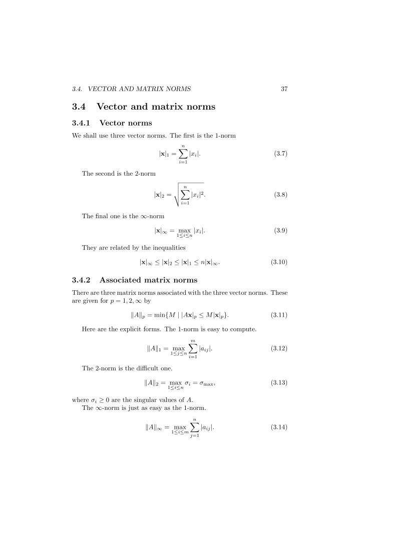
We shall use three vector norms. The first is the 1-norm

|x|1 =

n∑i=1

|xi|. (3.7)

The second is the 2-norm

|x|2 =

√√√√ n∑i=1

|xi|2. (3.8)

The final one is the ∞-norm

|x|∞ = max1≤i≤n

|xi|. (3.9)

They are related by the inequalities

|x|∞ ≤ |x|2 ≤ |x|1 ≤ n|x|∞. (3.10)

3.4.2 Associated matrix norms

There are three matrix norms associated with the three vector norms. Theseare given for p = 1, 2,∞ by

‖A‖p = min{M | |Ax|p ≤M |x|p}. (3.11)

Here are the explicit forms. The 1-norm is easy to compute.

‖A‖1 = max1≤j≤n

m∑i=1

|aij |. (3.12)

The 2-norm is the difficult one.

‖A‖2 = max1≤i≤n

σi = σmax, (3.13)

where σi ≥ 0 are the singular values of A.The ∞-norm is just as easy as the 1-norm.

‖A‖∞ = max1≤i≤m

n∑j=1

|aij |. (3.14)


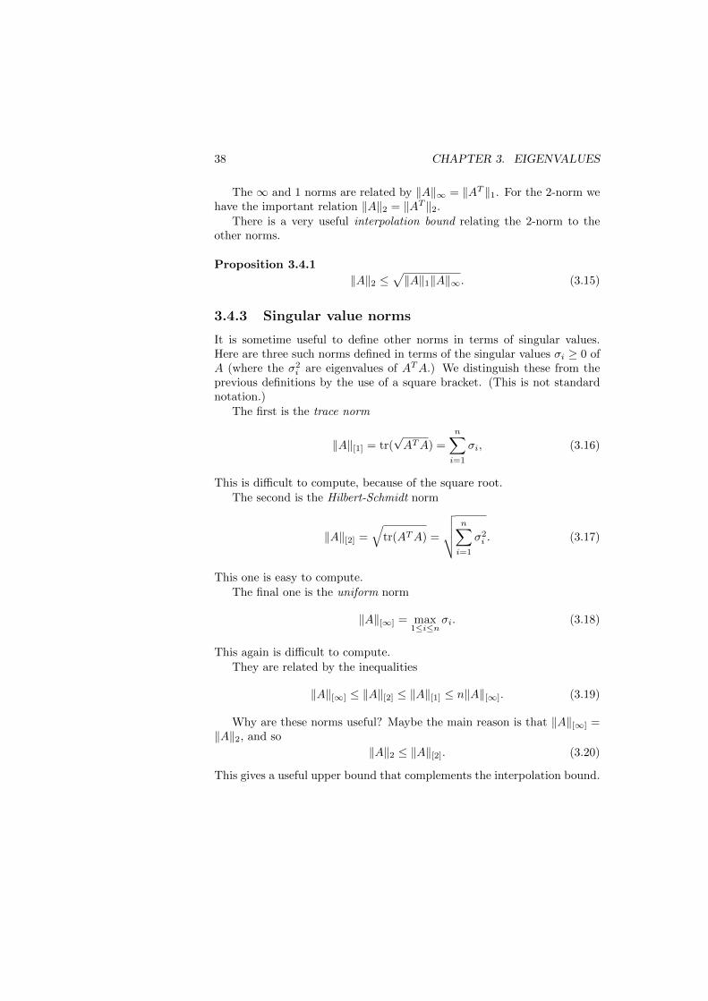
The ∞ and 1 norms are related by ‖A‖∞ = ‖AT ‖1. For the 2-norm wehave the important relation ‖A‖2 = ‖AT ‖2.

There is a very useful interpolation bound relating the 2-norm to theother norms.

Proposition 3.4.1

‖A‖2 ≤√‖A‖1‖A‖∞. (3.15)

3.4.3 Singular value norms

It is sometime useful to define other norms in terms of singular values.Here are three such norms defined in terms of the singular values σi ≥ 0 ofA (where the σ2

i are eigenvalues of ATA.) We distinguish these from theprevious definitions by the use of a square bracket. (This is not standardnotation.)

The first is the trace norm

‖A‖[1] = tr(√ATA) =

n∑i=1

σi, (3.16)

This is difficult to compute, because of the square root.The second is the Hilbert-Schmidt norm

‖A‖[2] =√

tr(ATA) =

√√√√ n∑i=1

σ2i . (3.17)

This one is easy to compute.The final one is the uniform norm

‖A‖[∞] = max1≤i≤n

σi. (3.18)

This again is difficult to compute.They are related by the inequalities

‖A‖[∞] ≤ ‖A‖[2] ≤ ‖A‖[1] ≤ n‖A‖[∞]. (3.19)

Why are these norms useful? Maybe the main reason is that ‖A‖[∞] =‖A‖2, and so

‖A‖2 ≤ ‖A‖[2]. (3.20)

This gives a useful upper bound that complements the interpolation bound.

3.4. VECTOR AND MATRIX NORMS 39

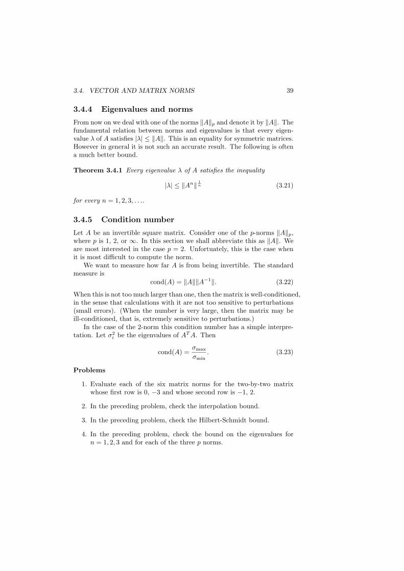
3.4.4 Eigenvalues and norms

From now on we deal with one of the norms ‖A‖p and denote it by ‖A‖. Thefundamental relation between norms and eigenvalues is that every eigen-value λ of A satisfies |λ| ≤ ‖A‖. This is an equality for symmetric matrices.However in general it is not such an accurate result. The following is oftena much better bound.

Theorem 3.4.1 Every eigenvalue λ of A satisfies the inequality

|λ| ≤ ‖An‖ 1n (3.21)

for every n = 1, 2, 3, . . ..

3.4.5 Condition number

Let A be an invertible square matrix. Consider one of the p-norms ‖A‖p,where p is 1, 2, or ∞. In this section we shall abbreviate this as ‖A‖. Weare most interested in the case p = 2. Unfortuately, this is the case whenit is most difficult to compute the norm.

We want to measure how far A is from being invertible. The standardmeasure is

cond(A) = ‖A‖‖A−1‖. (3.22)

When this is not too much larger than one, then the matrix is well-conditioned,in the sense that calculations with it are not too sensitive to perturbations(small errors). (When the number is very large, then the matrix may beill-conditioned, that is, extremely sensitive to perturbations.)

In the case of the 2-norm this condition number has a simple interpre-tation. Let σ2

i be the eigenvalues of ATA. Then

cond(A) =σmax

σmin. (3.23)

Problems

1. Evaluate each of the six matrix norms for the two-by-two matrixwhose first row is 0, −3 and whose second row is −1, 2.

2. In the preceding problem, check the interpolation bound.

3. In the preceding problem, check the Hilbert-Schmidt bound.

4. In the preceding problem, check the bound on the eigenvalues forn = 1, 2, 3 and for each of the three p norms.


5. Give an example of a matrix A for which the eigenvalue λ of largestabsolute value satisfies |λ| < ‖A‖ but |λ| = ‖An‖1/n for some n.

6. Prove the assertions about the concrete forms of the p-norms ‖A‖p,for p = 1, 2, ∞.

7. Prove that the 2-norm of a matrix is the 2-norm of its transpose.

3.5 Stability

3.5.1 Inverses

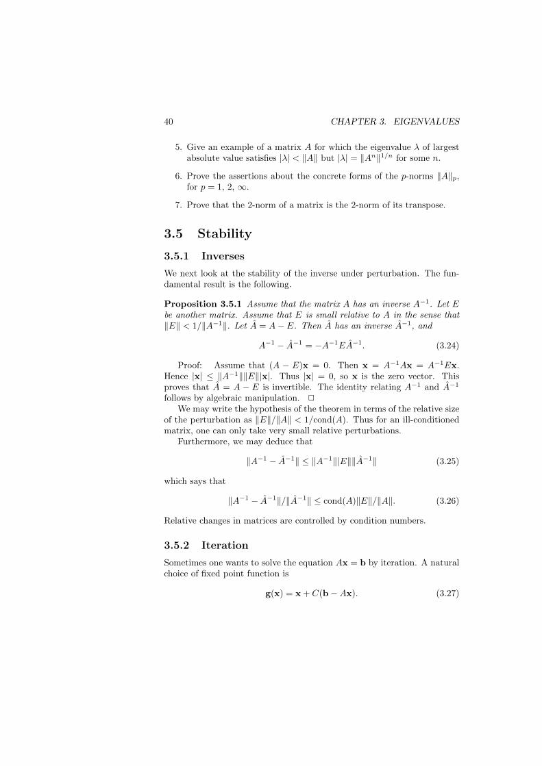
We next look at the stability of the inverse under perturbation. The fun-damental result is the following.

Proposition 3.5.1 Assume that the matrix A has an inverse A−1. Let Ebe another matrix. Assume that E is small relative to A in the sense that‖E‖ < 1/‖A−1‖. Let A = A− E. Then A has an inverse A−1, and

A−1 − A−1 = −A−1EA−1. (3.24)

Proof: Assume that (A − E)x = 0. Then x = A−1Ax = A−1Ex.Hence |x| ≤ ‖A−1‖‖E‖|x|. Thus |x| = 0, so x is the zero vector. Thisproves that A = A − E is invertible. The identity relating A−1 and A−1

follows by algebraic manipulation. 2

We may write the hypothesis of the theorem in terms of the relative sizeof the perturbation as ‖E‖/‖A‖ < 1/cond(A). Thus for an ill-conditionedmatrix, one can only take very small relative perturbations.

Furthermore, we may deduce that

‖A−1 − A−1‖ ≤ ‖A−1‖|E‖‖A−1‖ (3.25)

which says that

‖A−1 − A−1‖/‖A−1‖ ≤ cond(A)‖E‖/‖A‖. (3.26)

Relative changes in matrices are controlled by condition numbers.

3.5.2 Iteration

Sometimes one wants to solve the equation Ax = b by iteration. A naturalchoice of fixed point function is

g(x) = x + C(b−Ax). (3.27)

3.5. STABILITY 41

Here C can be an arbitrary non-singular matrix, and the fixed point willbe a solution. However for convergence we would like C to be a reasonableguess of or approximation to A−1.

When this is satisfied we may write

g(x)− g(y) = (I − CA)(x− y) = (A−1 − C)A(x− y). (3.28)

Then if ‖A−1 − C‖‖A‖ < 1, the iteration function is guaranteed to shrinkthe iterates together to a fixed point.

If we write the above condition in terms of relative error, it becomes‖A−1 − C‖/‖A−1‖ < 1/cond(A). Again we see that for an ill-conditionedmatrix one must make a good guess of the inverse.

3.5.3 Eigenvalue location

Let A be a square matrix, and let D be the diagonal matrix with the sameentries as the diagonal entries of A. If all these entries are non-zero, thenD is invertible. We would like to conclude that A is invertible.

Write A = DD−1A. The matrix D−1A has matrix entries aij/aii soit has ones on the diagonal. Thus we may treat it as a perturbation ofthe identity matrix. Thus we may write D−1A = I − (I −D−1A), whereI − D−1A has zeros on the diagonal and entries −aij/aii elsewhere. Weknow from our perturbation lemma that if I −D−1A has norm strictly lessthan one, then D−1A is invertible, and so A is invertible.

The norm that is most convenient to use is the ∞ norm. The conditionfor I−D−1A to have∞ norm strictly less than one is that maxi

∑j 6=i

|aij ||aii| <

1. We have proved the following result on diagonal dominance.

Proposition 3.5.2 If a matrix A satisfies for each i∑j 6=i

|aij | < |aii|, (3.29)

then A is invertible.

Let B be an arbitrary matrix and let λ be a number. Apply this resultto the matrix λI −B. Then λ is an eigenvalue of B precisely when λI −Bis not invertible. This gives the following conclusion.

Corollary 3.5.1 If λ is an eigenvalue of B, then for some i the eigenvalueλ satisfies

|λ− bii| ≤∑j 6=i

|bij |. (3.30)


The intervals about bii in the corollary are known as Gershgorin’s disks.Problems

1. Assume Ax = b. Assume that there is a computed solution x = x−e,where e is an error vector. Let Ax = b, and define the residual vectorr by b = b− r. Show that |e|/|x| ≤ cond(A)|r|/|b|.

2. Assume Ax = b. Assume that there is an error in the matrix, sothat the matrix used for the computation is A = A − E. Take thecomputed solution as x defined by Ax = b. Show that |e|/|x| ≤cond(A)‖E‖/‖A‖.

3. Find the Gershgorin disks for the three-by-three matrix whose firstrow is 1, 2, −1, whose second row is 2, 7, 0, and whose third row is−1, 0, −5.

3.6. POWER METHOD 43

3.6 Power method

We turn to the computational problem of finding eigenvalues of the squarematrix A. We assume that A has distinct real eigenvalues. The powermethod is a method of computing the dominant eigenvalue (the eigenvaluewith largest absolute value).

The method is to take a more or less arbitrary starting vector u andcompute Aku for large k. The result should be approximately the eigen-vector corresponding to the dominant eigenvalue.

Why does this work? Let us assume that there is a dominant eigenvalueand call it λ1. Let u be a non-zero vector. Expand u =

∑i cixi in the

eigenvectors of A. Assume that c1 6= 0. Then

Aku =∑i

ciλki xi. (3.31)

When k is large, the term c1λk1xi is so much larger than the other terms

that Aku is a good approximation to a multiple of x1.[We can write this another way in terms of the spectral representation.

Let u be a non-zero vector such that yT1 u 6= 0. Then

Aku = λk1x1yT1 u +

∑i6=1

λki xiyTi u. (3.32)

When k is large the first term will be much larger than the other terms.Therefore Aku will be approximately λk1 times a multiple of the eigenvectorx1.]

In practice we take u to be some convenient vector, such as the firstcoordinate basis vector, and we just hope that the condition is satisfied.We compute Aku by successive multiplication of the matrix A times theprevious vector. In order to extract the eigenvalue we can compute theresult for k+ 1 and for k and divide the vectors component by component.Each quotient should be close to λ1.Problems

1. Take the matrix whose rows are 0, −3 and −1, 2. Apply the matrixfour times to the starting vector. How close is this to an eigenvector.

2. Consider the power method for finding eigenvalues of a real matrix.Describe what happens when the matrix is symmetric and the eigen-value of largest absolute value has multiplicity two.

3. Also describe what happens when the matrix is not symmetric andthe eigenvalues of largest absolute value are a complex conjugate pair.


3.7 Inverse power method

The inverse power method is just the power method applied to the matrix(A− µI)−1. We choose µ as an intelligent guess for a number that is nearbut not equal to an eigenvalue λj . The matrix has eigenvalues (λi − µ)−1.If µ is closer to λj than to any other λi, then the dominant eigenvalue of(A − µI)−1 will be (λj − µ)−1. Thus we can calculate (λj − µ)−1 by thepower method. From this we can calculate λj .

The inverse power method can be used to search for all the eigenvalues ofA. At first it might appear that it is computationally expensive, but in factall that one has to do is to compute an LU or QR decomposition of A−µI.Then it is easy to do a calculation in which we start with an arbitraryvector u and at each stage replace the vector v obtained at that stage withthe result of solving (A− µI)x = v for x using this decomposition.Projects

1. Write a program to find the dominant eigenvalue of a matrix by theinverse power method.

2. Find the eigenvalues of the symmetric matrix with rows 16, 4, 1, 1and 4, 9, 1, 1 and 1, 1, 4, 1 and 1, 1, 1, 1.

3. Change the first 1 in the last row to a 2, and find the eigenvalues ofthe resulting non-symmetric matrix.

3.8 Power method for subspaces

The power method for subspaces is very simple. One computes Ak for largek. Then one performs a decomposition Ak = QR. Finally one computesQ−1AQ. Miracle: the result is upper triangular with the eigenvalues onthe diagonal!

Here is why this works. Take e1, . . . , er to be the first r unit basisvectors. Then ei =

∑j cijxj , where the xj are the eigenvectors of A corre-

sponding to the eigenvalues ordered in decreasing absolute value. Thus forthe powers we have

Akei =∑j

cijλkjxj . (3.33)

To a good approximation, the first r terms of this sum are much larger thanthe remaining terms. Thus to a good approximation the Akei for 1 ≤ i ≤ rare just linear combinations of the first r eigenvectors.

We may replace the Akei by linear combinations that are orthonormal.This is what is accomplished by the QR decomposition. The first r columns

3.8. POWER METHOD FOR SUBSPACES 45

of Q are an orthonormal basis consisting of linear combinations of the Akeifor 1 ≤ i ≤ r.

It follows that the first r columns of Q are approximately linear combi-nations of the first r eigenvectors. If this were exact, then Q−1AQ wouldbe the exact Schur decomposition. However in any case it should be a goodapproximation.

[This can be considered in terms of subspaces as an attempt to applythe power method to find the subspace spanned by the first r eigenvectors,for each r. The idea is the following. Let Vr be a subspace of dimensionr chosen in some convenient way. Then, in the typical situation, the firstr eigenvectors will have components in Vr. It follows that for large k thematrix Ak applied to Vr should be approximately the subspace spanned bythe first r eigenvectors.

However we may compute the subspace given by Ak applied to Vr byusing the QR decomposition. Let

Ak = QkRk (3.34)

be the QR decomposition of Ak. Let Vr be the subspace of column vectorswhich are non-zero only in their first r components. Then Rk leaves Vrinvariant. Thus the image of this Vr by Qk is the desired subspace.

We expect from this that Qk is fairly close to mapping the space Vr intothe span of the first r eigenvectors. In other words, if we define Uk+1 by

Uk+1 = Q−1k AQk, (3.35)

then this is an approximation to a Schur decomposition. Thus one shouldbe able to read off all the eigenvalues from the diagonal.]

This method is certainly simple. One simply calculates a large powerof A and finds the QR decomposition of the result. The resulting orthogo-nal matrix give the Schur decomposition of the original A, and hence theeigenvalues.

What is wrong with this? The obvious problem is that Ak is an ill-conditioned matrix for large k, and so computing the QR decomposition isnumerically unstable. Still, the idea is appealing in its simplicity.

Problems

1. Take the matrix whose rows are 0, −3 and −1, 2. Take the eigenvectorcorresponding to the largest eigenvalue. Find an orthogonal vectorand form an orthogonal basis with these two vectors. Use the matrixwith this basis to perform a similarity transformation of the originalmatrix. How close is the result to an upper triangular matrix?


2. Take the matrix whose rows are 0, −3 and −1, 2. Apply the matrixfour times to the starting vector. Find an orthogonal vector and forman orthogonal basis with these two vectors. Use the matrix with thisbasis to perform a similarity transformation of the original matrix.How close is the result to an upper triangular matrix?

3.9 QR method

The famous QR method is just another variant on the power method forsubspaces of the last section. However it eliminates the calculational diffi-culties.

Here is the algorithm. We want to find approximate the Schur decom-position of the matrix A.

Start with U1 = A. Then iterate as follows. Having defined Uk, write

Uk = QkRk, (3.36)

where Qk is orthogonal and Rk is upper triangular. Let

Uk+1 = RkQk. (3.37)

(Note the reverse order). Then for large k the matrix Uk+1 should be a goodapproximation to the upper triangular matrix in the Schur decomposition.

Why does this work?First note that Uk+1 = RkQk = Q−1

k UkQk, so Uk+1 is orthogonal similarto Uk.

Let Qk = Q1 · · ·Qk and Rk = Rk · · ·R1. Then it is easy to see that

Uk+1 = Q−1k AQk. (3.38)

Thus Uk+1 is similar to the original A.Furthermore, QkRk = Qk−1UkRk−1 = AQk−1Rk−1. Thus the kth stage

decomposition is produced from the previous stage by multiplying by A.Finally, we deduce from this that

QkRk = Ak. (3.39)

In other words, the Qk that sets up the similarity of Uk+1 with A is the sameQk that arises from the QR decompositon of the power Ak. But we haveseen that this should give an approximation to the Schur decomposition ofA. Thus the Uk+1 should be approximately upper triangular.Projects

1. Implement the QR method for finding eigenvalues.

3.10. FINDING EIGENVALUES 47

2. Use the program to find the eigenvalues of the symmetric matrix withrows 1, 1, 0, 1 and 1, 4, 1, 1 and 0, 1, 9, 5 and 1, 1, 5, 16.

3. Change the last 1 in the first row to a 3, and find the eigenvalues ofthe resulting non-symmetric matrix.

3.10 Finding eigenvalues

The most convenient method of finding all the eigenvalues is the QR method.Once the eigenvalues are found, then the inverse power method gives an easydetermination of eigenvectors.

There are some refinements of the QR method that give greater effi-ciency, especially for very large matrices.

The trick is to work with Hessenberg matrices, which are matrices withzeros below the diagonal below the main diagonal.

The idea is to do the eigenvalue determination in two stages. The firststage is to transform A to Q−1AQ = A, where A is a Hessenberg matrix.This is an orthogonal similarity transformation, so this gives a matrix Awith the same eigenvalues.

This turns out to be an easy task. The idea is much the same as the ideafor the QR decomposition, except that the reflections must be applied onboth sides, to make it an orthogonal similarity transformation. No limitingprocess is involved.

One builds the matrix Q out of reflection matrices, Q = Pn · · ·P1. Atthe jth stage the matrix is Pj · · ·P1AP1 · · ·Pj . The unit vector determiningthe reflection Pj is taken to be zero in the first j components. Furthermoreit is chosen so that application of Pj on the left will zero out the componentsin the jth column below the entry below the diagonal entry. The entry justbelow the diagonal entry does not become zero. However the advantage isthat the application of Pj on the right does not change the jth column orany of the preceding columns.

Now that the matrix is in Hessenberg form, we note that the QR algo-rithm preserves Hessenberg form. We take the first U1 = A, which is inHessenberg form. Then we may easily compute that

Uk+1 = RkUkR−1k . (3.40)

Thus each Uk is in Hessenberg form, since Hessenberg form is preserved bymultiplication by upper triangular matrices.

This is very advantageous, since at each stage we must decompose Uk =QkRk and then multiply out RkQk. Since Uk is in Hessenberg form, the


reflection vectors used in the decomposition are each vectors that have onlytwo non-zero components. The arithmetic is much reduced.

æ

Chapter 4

Nonlinear systems

4.1 Introduction

This chapter deals with solving equations of the form f(x) = 0, where f isa continuous function from Rn to Rn. It also treats questions of roundofferror and its amplification in the course of a numerical calculation.

In much of what we do the derivative f ′ of such a function f will playan essential role. This is defined in such as way that

f(x + h)− f(x) = f ′(x)h + r, (4.1)

where the remainder is of higher than first order in the vector h. Thus thederivative f ′(x) is a matrix. If we write this in variables with y = f(x),then the derivative formula is

∆y ≈ f ′(x)∆x. (4.2)

If we write these relations in components, we get

fi(x + h) = fi(x) +

n∑j=1

∂fi(x)

∂xjhj + ri. (4.3)

Thus the derivative matrix is the matrix of partial derivatives. Using vari-ables one writes

∆yi ≈n∑j=1

∂yi∂xj

∆xj . (4.4)

The same idea is often expressed in differential notation

dyi =

n∑j=1

∂yi∂xj

dxj . (4.5)

49

50 CHAPTER 4. NONLINEAR SYSTEMS

There are several interpretations of such a function. Two of the mostimportant are the interpretation as a transformation and the interpretationas a vector field.

When we think of a function g as a transformation, we may think ofx as being a point in one space and y = g(x) as being a point in someother space. For each x there is a corresponding y. It is illuminating tolook at the consequence of a change of coordinate system. Say that wehave z coordinates that are functions of the x coordinates, and we have wcoordinates that are functions of the y coordinates. In that case we have

∂wi∂zj

=∑k

∂wi∂yk

∑r

∂yk∂xr

∂xr∂zj

. (4.6)

This says that the new derivative matrix is obtained from the original ma-trix by multiplying on each side by matrices representing the effect of thecoordinate transformations.

A variant is when we think of the function as a transformation from aspace to the same space. In that case we may write x = g(x) and think ofx as the coordinates of the original point and x as the coordinates of thenew point.

In this case there is only the change from x to z coordinates, so thechange of variable formula becomes

∂zi∂zj

=∑k

∂zi∂xk

∑r

∂xk∂xr

∂xr∂zj

. (4.7)

We shall see in the problems that there is a special situation when thischange is a familiar operation of linear algebra.

When we think of a function f as a vector field, then we think of x asbeing a point in some space and y = f(x) as being the components of avector attached to the point x.

Let us look at the effect of a change of coordinates on the vector fielditself. We change from x to z coordinates. Let us call the new componentsof the vector field y. Then if we look at a curve tangent to the vector field,we see that along the curve

yi =dzidt

=∑k

∂zi∂xk

dxkdt

=∑k

∂zi∂xk

yk. (4.8)

So the vector field is changed by multiplication on the left by a matrix:

yi =∑k

∂zi∂xk

yk. (4.9)

4.2. DEGREE 51

How about the partial derivatives of the vector field? Here the situationis ugly. A routine computation gives

∂yi∂zj

=∑r

∑k

[∂2zi

∂xr∂xkyk +

∂zi∂xk

∂yk∂xr

]∂xr∂zj

. (4.10)

This does not even look like matrix multiplication. We shall see in theproblems that there is a special situation where this difficulty does notoccur and where we get instead some nice linear algebra.Problems

1. Consider a transformation x = g(x) of a space to itself. Show thatat a fixed point the effect of a change of coordinates on the derivativematrix is a similarity transformation.

2. Consider a vector field with components y = f(x) in the x coordinatesystem. Show that at a zero of the vector field the effect of a changeof coordinates on the derivative matrix is a similarity transformation.

4.2 Degree

The intermediate value theorem was a fundamental result in solving equa-tions in one dimension. It is natural to ask whether there is an analog ofthis theorem for systems. There is such an analog; one version of it is thefollowing topological degree theorem.

We say that a vector y is opposite to another vector x if there existsc ≥ 0 with y = −cx.

Theorem 4.2.1 Let f be a continuous function on the closed unit ball Bin Rn with values in Rn. Let ∂B be the sphere that is the boundary of B.Assume that for each x in ∂B the vector f(x) is not opposite to x. Thenthere exists a point r in B such that f(r) = 0.

This is called a topolological degree theorem because there is an invari-ant called the degree which under the hypotheses of this theorem has thevalue one. In general, if the degree is non-zero, then there is a fixed point.

The proof of this theorem is much more difficult than the proof of theintermediate value theorem, and it will not be attempted here.

When n = 1 we are essentially in the situation of the intermediate valuetheorem. The unit ball B is the closed interval [−1, 1], and the boundary∂B consists of the two points −1 and 1. The computational problem thusconsists of checking the value of a function on these two end points.


Unfortunately, the theorem does not lead to a particularly efficient com-puter implementation when n > 1. (However perhaps something can bedone when n = 2.) The problem is that the boundary ∂B is an infinite set,and one has to do a calculation involving the whole boundary to check thepresence of a root.Problems

1. Show how to derive the intermediate value theorem as a corollary ofthe degree theorem.

2. Find a example in two dimensions where the degree theorem appliesto guarantee the existence of the root, but where the root cannot becalculated by elementary means.

4.2.1 Brouwer fixed point theorem

The degree theorem has implications for the existence of fixed points. Themost famous such result is the Brouwer fixed point theorem.

Theorem 4.2.2 Let g be a continuous function on the closed unit ball Bin Rn with values in Rn. Let ∂B be the sphere that is the boundary of B.Assume g sends ∂B into B. Then g has a fixed point.

Proof: Let f(x) = x−g(x) defined on the closed unit ball B. We wantto show that for some x in B the vector f(x) = 0.

Suppose that for all x in B the vector f(x) 6= 0. Then g maps ∂B intothe interior of the unit ball. Consider x in ∂B. If f(x) is opposite to x,then g(x) = (1 + c)x with c ≥ 0, which is impossible. Therefore f(x) isnever opposite to x. But then the degree theorem leads to a contradiction.2

Unfortunately, this proof only reduces the Brouwer theorem to the de-gree theorem, and does not provide a self-contained proof. Again the ap-paratus of algebraic topology is necessary for a satisfactory treatment.

Two subsets Rn are homeomorphic if there is a one-to-one correspon-dence between them that is continuous in both directions. The Brouwerfixed point theorem applies to a subset that is homeomorphic to the closedunit ball. Thus it applies to a closed ball of any size, or to a closed cube.

4.3 Iteration

4.3.1 First order convergence

Another approach to numerical root-finding is iteration. Assume that g isa continuous function. We seek a fixed point r with g(r) = r. We can

4.3. ITERATION 53

attempt to find it by starting with an x0 and forming a sequence of iteratesusing xn+1 = g(xn).

Theorem 4.3.1 Let g be continuous and let xn a sequence such that xn+1 =g(xn). Then if xn → r as n→∞, then g(r) = r.

This theorem shows that we need a way of getting sequences to converge.In higher dimensions the most convenient approach is to have a bound onthe derivative.

How do we use such a bound? We need a replacement for the meanvalue theorem. Here is the version that works.

Lemma 4.3.1 Let g be a function with continuous derivative g′. Then

|g(y)− g(x)| ≤ max0≤t≤1

‖g′(zt)‖ |y − x|, (4.11)

where zt = (1− t)x + ty lies on the segment between x and y.

The way to prove the lemma is to use the identity

g(y)− g(x) =

∫ 1

0

g′(zt)(y − x) dt. (4.12)

Theorem 4.3.2 Let B be a set that is homeomorphic to a closed ball.Assume that g is continuous on B and that g maps B into itself. Then ghas a fixed point. Assume also that B is convex and that ‖g′(z)‖ ≤ K < 1for all z in B. Let x0 be in B and iterate using xn+1 = g(xn). Thenthe iterates converge to the fixed point. Furthermore, this fixed point is theunique fixed point in B.

Proof: The Brouwer theorem guarantees that there is a fixed point rin the interval. By the mean value theorem, for each x we have xn+1− r =g(xn) − g(r). By the lemma the norm of this is bounded by K times thenorm of x− r. In other words each iteration replacing x by g(x) brings uscloser to r. 2

We see that that r is a stable fixed point if ‖g′(r)‖ < 1. However thereis a stronger result. Recall that the power of a matrix has a norm that givesa much better bound on the eigenvalues. We may compute the derivative ofthemth iterate gm(x) and we get g′(gm−1(x))g′(gm−2(x)) · · ·g′(g(x))g′(x).At the fixed point with g(r) = r this is just the power g′(r)m. So near thefixed point we expect that

xn+m − r = gm(xn)− gm(r) ≈ g′(r)m(xn − r). (4.13)

We see that if ‖g(r)m‖ < 1 then the fixed point r is stable.If we want to use this to solve f(x) = 0, we can try to take g(x) = x−

Cf(x) for some suitable matrix K. If C is chosen so that g′(x) = 1−Cf ′(x)is small for x near r, then there should be a good chance of convergence.


4.3.2 Second order convergence

Since the speed of convergence in iteration with g is controlled by g′(r), itfollows that the situation when g′(r) = 0 is going to have special properties.

It is possible to arrange that this happens. Say that one wants to solvef(x) = 0. Newton’s method is to take g(x) = x− f ′(x)−1f(x). It is easy tocheck that f(r) = 0 and f ′(r) non-singular imply that g′(r) = 0.

Newton’s method is not guaranteed to be good if one begins far fromthe starting point. The damped Newton method is more conservative. Onedefines g(x) as follows. Let m = f ′(x)−1f(x) and let y = x −m. While|f(y)| ≥ |f(x)| replace m by m/2 and let y = x−m. Let g(x) be the finalvalue of y.Projects

1. Newton’s method for systems has the disadvantage that one mustcompute many partial derivatives. Steffensen’s method provides analternative. The method is to iterate with g(x) = x − w, where wis the solution of J(x)w = f(x). For Newton’s method J(x) = f ′(x),but for Steffensen’s method we approximate the matrix of partialderivatives by a matrix of difference quotients. Thus the i, j entry ofJ(x) is (fi(x + hjej)− fi(x))/hj), where hj = αj(f(x)). Here α is afunction that vanishes at zero. Thus as f(x) approaches zero, thesedifference quotients automatically approach the partial derivatives.

There are various possible choices for the function α. One popularchoice is the identity αj(z) = zj , so that hj = fj(x). The disadvan-tage of this choice is that hj can be zero away from the root.

Another method is to take each component of α to be the length, sothat αj(z) = |z| and hj = |f(x)|. This choice of α is not differentiableat the origin, but in this case this is not a problem.

Perhaps an even better method is to take αj(z) to be the minimumof |z| and some small number, such as 0.01. This will make thedifference matrix somewhat resemble the derivative matrix even farfrom the solution.

The project is to write a program for solving a system of non-linearequations by Steffensen’s method. Try out the program on a simplesystem for which you know the solution.

2. Use the program to solve the following system.

x3 − 3xy2 − 6z3 + 18zw2 − 1 = 0

3x2y − y3 − 18z2w + 6w3 = 0

4.3. ITERATION 55

xz − yw − 1 = 0

yz + xw = 0

Find a solution near the point where (x, y, z, w) is (0.6, 1.1, 0.4,−0.7).

Problems

1. Let B be the ball of radius r centered at c. Assume that ‖g′(z)‖ ≤K < 1 for all z in B. Suppose that a is in B and that a and g(a)satisfy Kr +K|a− c|+ |g(a)− c| ≤ r. Show that g maps B into B.

2. Let g(x) = x − Cf(x). Show that if C approximates f ′(x)−1 in thesense that ‖C − f ′(x)−1‖‖f ′(x)‖ is bounded below one near the fixedpoint, then iteration with g starting near the fixed point converges tothe fixed point.

3. Calculate g′(x) in Newton’s method.

4. Show that in Newton’s method f(r) = 0 with f ′(r) invertible impliesg′(r) = 0.

5. The following problems deal with the theory of Steffensen’s method.For simplicity we deal with the scalar case. Thus the method con-sists of iteration with g(x) = x − f(x)/m(x), where m(x) = (f(x +α(f(x)))−f(x))/α(f(x)). The function α is chosen so that α(0) = 0.Let r be a root of f , so that f(r) = 0, and assume that f ′(r) 6= 0.The first problem is to compute m(r) and m′(r).

6. Show that g′(r) = 0 and that g′′(r) = (2m′(r)− f ′′(r))/f ′(r).

7. Let xn+1 = g(xn) and assume xn → r as n to ∞. Evaluate the limitof (xn+1 − r)/(xn − r)2 as n→∞.

8. What if α(z) = |z|, so that α is not differentiable at 0. Is it still truethat g′(r) = 0.

9. Another interesting problem is to examine the situation when theiterations give increasing or decreasing sequences of vectors. Showthat if the matrix f ′(x)−1 has positive entries and f(x) has positiveentries, then g(x) ≤ x.

10. This leads to the problem of finding when a matrix A has the propertythat A−1 has positive entries. Show that if A = D − N , whereD is diagonal and N is off-diagonal and D ≥ 0 and N ≥ 0 and‖D−1N‖∞ < 1, then A−1 has only positive entries.


11. Show that if in this situationA−1 exists but we have only ‖D−1N‖∞ ≤1, then the same conclusion holds.

12. Assume that x ≥ r implies f(x) ≥ 0. We want to see when x ≥ rimplies g(x) ≥ r. Evaluate g′(z) terms of f ′′(z) and show that it issufficient that all the second partial deriviatives in this expression arepositive.

4.4 Power series

Let C be a matrix with ‖C‖ < 1. Then (1 − C)−1 exists. We may mosteasily see this by expanding C in a power series. By summing this serieswe see that ‖(1− C)−1‖ ≤ 1/(1− ‖C‖).

Recall that in general ‖Ck‖ ≤ ‖C‖k. Thus there is an interesting gen-eralization to the case when ‖Ck‖ < 1 for some k. We observe that

(1− C)−1 = (1 + C + C2 + · · ·+ Ck−1)(1− Ck)−1. (4.14)

It follows that also in this situation (1− C)−1 exists.Problems

1. Find a bound for (1 + C)−1 in terms of ‖C‖ and ‖Ck‖.

2. Show that if A−1 exists and ‖(EA−1)k‖ < 1 for some k, then (A −E)−1 exists.

4.5 The spectral radius

The spectral radius ρ(A) of a square matrix A is the maximum absolutevalue of an eigenvalue. Even if the matrix is real, it is important in thisdefinition that all complex eigenvalues are considered. The reason for thisimportance is that with this definition we have the following theorem.

Theorem 4.5.1 The norms of powers An and the spectral radius of A arerelated by

limn→∞

‖An‖ 1n = ρ(A). (4.15)

Proof:It is easy to see that for all n it is true that ρ(A) ≤ ‖An‖ 1

n . The problemis to show that for large n the right hand side is not much larger than theleft hand side.

4.6. LINEAR ALGEBRA REVIEW 57

The first thing to do is to check that |z| < 1/ρ(A) implies that (I−zA)−1

exists. (Otherwise 1/z would be an eigenvalue of A outside of the spectralradius.)

The essential observation is that (I − zA)−1 is an analytic function ofz for |z| < 1/ρ(A). It follows that the power series expansion convergesin this disk. Thus for |z| with |z| < 1/ρ(A) there is a constant c with‖(zA)n‖ = |z|n‖An‖ ≤ c.

We have shown that for every r < 1/ρ(A) there is a c with ‖An‖ 1n ≤

c1n /r. Take 1/r to be larger than but very close to ρ(A). Take n so large

that c1n /r is still close to ρ(A). Then ‖An‖ must be larger than but close

to ρ(A). 2

Let us look at this proof in more detail. The essential point is theconvergence of the power series. Why must this happen? It is a miracle ofcomplex variable: the Cauchy integral formula reduces the convergence ofan arbitrary power series inside its radius of convergence to the convergenceof a geometric series.

Look at the Cauchy integral formula

(I − wA)−1 =1

2πi

∫(1− zA)−11/(z − w) dz, (4.16)

where w is inside the circle of integration |z| = r and r < 1/ρ(A). We mayexpand in a geometric series in powers of w/z. From this we see that thecoefficients of the expansion in powers of w are

An =1

2πi

∫(1− zA)−11/zn+1 dz. (4.17)

This proves that ‖An‖ ≤ c/rn, where

c =1

2πr

∫‖(I − zA)−1‖ d|z| (4.18)

over |z| = r.Notice that as r approaches 1/ρ(A) the bound c will become larger, due

to the contribution to the integral from the singularity at z = 1/λ.Problems

1. Show that it is false in general that ρ(A + B) ≤ ρ(A) + ρ(B). Hint:Find 2 by 2 matrices for which the right hand side is zero.

4.6 Linear algebra review

We briefly review the various similarity representations of matrices. We areinterested in the case of a real square matrix A.


There is always a (possibly complex) matrix S and a (possibly complex)upper triangular matrix J such that S−1AS = J . Thus A has the Jordanrepresentation A = SJS−1. The eigenvalues of A occur on the diagonal ofJ .

Assume that A has distinct eigenvalues. Then the eigenvectors of Aform a basis. Then there is always a (possibly complex) matrix S and a(possibly complex) diagonal matrix D such that S−1AS = D. Thus A hasthe spectral representation A = SDS−1. The eigenvalues of A occur on thediagonal of D. The eigenvectors form the columns of the matrix S.

Assume that A has real eigenvalues (not necessarily distinct). Thenthere is always an orthogonal matrix Q and an upper triangular matrix Usuch that Q−1AQ = U . Thus A has the Schur representation A = QUQ−1

where Q−1 = QT . The eigenvalues of A occur on the diagonal of U .Assume that A is symmetric, so A = AT . Then A has real eigenvalues

(not necessarily distinct). The eigenvectors of A may be chosen so as toform an orthonormal basis. There is always an orthogonal matrix Q anda diagonal matrix D such that Q−1AQ = D. Thus A has the spectralrepresentation A = QDQ−1 where Q−1 = QT . The eigenvalues of A occuron the diagonal of D. The eigenvectors may be chosen to form the columnsof the matrix Q.

4.7. ERROR ANALYSIS 59

4.7 Error analysis

There are several sources of error in numerical analysis. There are somethat are obvious and inescapable, such as the input error in data from theoutside world, and the inherent representation error in the precision thatis available in the output.

4.7.1 Approximation error and roundoff error

However there are two main sources of error. One is the approximationerror. This is the error that is due to approximating limits by finite arith-metical operators. It is sometimes called truncation error and sometimescalled discretization error, depending on the context.

The most common tool for treating approximation error is Taylor’sformula with remainder. The idea is that a function such as f(x) =f(a) + f ′(a)(x − a) + 1/2f ′′(a)(x − a)2 + r is approximated by a poly-nomical p(x) = f(a) + f ′(a)(x − a) + 1/2f ′′(a)(x − a)2. The advantageis that the polynomial can be computed by addition and multiplication,which are operations supported by the computer. The disadvantage is thatthere is an error r. One hopes that the error r is small, and that one canprove that it is small.

There are other forms of approximation error, but in every case thechallenge is to find algorithms for which the approximation error is small.This is a general mathematical problem, perhaps the central problem inanalysis. In this respect numerical analysis appears as nothing more thana subset of analysis.

Of course some parts of numerical analysis have no approximation error.For instance, the formulas for inverting a matrix using the LU or QRdecomposition are exact.

Examples that we have encountered where there is approximation errorare root-finding and eigenvalue computation. In each of these cases thecomputation is only exact when one performs infinitely many iterations,which is impossible on the computer.

The other main source of error is roundoff error. This is due to thefact that computer does not do exact arithmetic with real numbers, butonly floating point arithmetic. This source of error is peculiar to numericalanalysis.

4.7.2 Amplification of absolute error

We want an algorithm to have the property that it does not magnify round-off error needlessly. For a start we do an analysis of absolute error.


For the purposes of analysis, imagine that we want to compute a func-tion y = f(x). Then dy = f ′(x)dx, so small input error is amplified by theentries in the matrix f ′(x). If this matrix has large entries, then the prob-lem in inherently ill-conditioned with respect to absolute error. Nothingcan be done to remedy this.

Example: Consider the problem of solving a polynomial equation p(z) =0. The roots are functions of the coefficients. Let a be one of the coefficients,say the coefficient of zm. Then the root y satisfies an equation p(y) =P (a, y) = 0. Differentiate this equation with respect to a. We obtainym + p′(y)dy/da = 0, where p′(z) is the derivative of the polynomial withrespect to z. This shows that the problem of finding the root y as a functionof the coefficient a is not well-posed when p′(y) = 0, that is, when y is amultiple root.

However, even if the problem is well-conditioned, a poor choice of al-gorithm can give trouble. Say that our numerical algorithm is to computez = h(x) and then y = g(z). Then we have an intermediate stage at whichwe can introduce roundoff errors. We have dy = g′(z)dz, so if g′(z) is large,which can happen, then we can have these intermediate errors amplified.

We can examine this amplification effect rather crudely in terms of thenorm of the matrix g′(z). Or we can write out the entries explicitly as

dyi =∑k

∂yi∂zk

dzk (4.19)

and perform a detailed analysis.From the chain rule, we always have f ′(x) = g′(z)h′(x). So, roughly

speaking, for a fixed problem of computing f(x), we want to choose analgorithm so as to take g′(z) to have a reasonably small norm, not greatlyexceeding the norm of f ′(x). This keeps the norm of h′(x) from beingsmall, but this norm does not matter. (The whole point is not to needlesslyamplify roundoff errors from intermediate stages.)

We say that an algorithm is numerically stable if the errors that areintroduced from intermediate stages are not much larger than the inherentroundoff errors that arize from the input error and the representation error.

A problem can be well-conditioned, but we can make the mistake ofchoosing a numerically unstable algorithm. This leads to wrong answers!

Example: Here is a classic example. Say that one wants to compute thefunction y = f(x) =

√x+ 1−

√x for large x. One does this in stages. The

first stage is to compute z =√x+ 1 and w =

√x. (Note that z2 − w2 =

1.) The second stage may be performed in two ways. The obvious butundesirable way is to compute y = z − w. The better way is to computey = 1/(z + w).

4.7. ERROR ANALYSIS 61

The derivative dy/dx is very small when x is large. Errors in x aredamped. However in the undesirable method ∂y/∂z = 1 and ∂y/∂w = −1,which are not small. So errors in z and w are not damped.

With the better method, the partial derivatives are ∂y/∂z = −1/(z+w)2

and ∂y/∂w = −1/(z + w)2. Errors in z and w are damped. Clearly thismethod is preferable.

Example: Fix 0 < a < 1. Let b = a + 1/a. Consider the problem ofsolving the recurrence relation xn+1 = bxn−xn−1 with x1 = a and x0 = 1.It is easy to see that the solution is xk = ak. Clearly dxk/da = kak−1 issmall. The problem is well-posed.

However the recurrence relation is a terrible way to compute the answer.The reason is that this is essentially computing the matrix power in(

xk+1

xk

)=

(b −11 0

)k (a1

). (4.20)

The largest eigenvalue of the matrix is 1/a > 1, so for large k this has verylarge norm. Errors (from earlier stages of taking the power) are very muchamplified!

4.7.3 Amplification of relative error

The arithmetic used in most computers is floating point arithmetic, so theroundoff error is more or less independent of the size of the number. Itshould be thought of as a relative error. Thus the amplification effect ofrelative error is what is actually important.

The formula for the dependence of relative error in the output on relativeerror in an intermediate stage is

dyiyi

=∑k

zkyi

∂yi∂zk

dzkzk

. (4.21)

It is of course possible to think of this as the formula for the absoluteerror amplifiation for logarithms

d log |yi| =∑k

∂ log |yi|∂ log |zk|

d log |zk|. (4.22)

In this sense it falls under the scope of the analysis of the previous section.Ultimately, however, the result is that the amplification of relative error

is given by a matrix with entries (zk/yi)(∂yi/∂zk). We want this to be asmall matrix. We have no control over the yi, since this is simply the outputvalue. But the algorithm controls the size of the intermediate number zk.


The conclusion is that, unless there is a compensating small derivative, weprefer small sizes of the numbers zk that occur in intermediate steps of thecomputation.

Example: Say that one wants to compute y = f(x) = x+ 2 at x = 2. Abad algorithm is to compute z = 1000001x and w = 1000000x and computey = z − w + 2. The reason is that a relative error of a millionth in z or wwill give a completely wrong answer. Big numbers have been introducedneedlessly.

Example: Say that one wants to compute y = f(x) = x + 2 at x = 2.One algorithm is to compute z = 1000000x and then y = 1/1000000z + 2.This introduces a big number z, but in this case it does no harm. Thereason is that the small dy/dz compensates the large z.

Example: Let us repeat the example of the function f(x) =√x+ 1 −√

x, this time making the analysis using relative error. The first stage is tocompute z =

√x+ 1 and w =

√x. (Note that z2 − w2 = 1.) The second

stage may be performed in two ways. The obvious but undesirable way isto compute y = z − w. The better way is to compute y = 1/(z + w).

The relative error amplification inherent in the problem is (x/y)dy/dxwhich evaluates to −x/(zw), a quantity bounded by one. The problem iswell-conditioned.

However in the undesirable method we have (z/y)∂y/∂z = z(z+w) andalso (w/y)∂y/∂w = −w(z + w), which are very large. So relative errors inz and w are amplified.

With the better method, the partial derivatives are given by the expres-sions (z/y)∂y/∂z = −z/(z+w) and (w/y)∂y/∂w = −w/(z+w). This doesnot amplify relative error, and so this method is numerically stable. Notethat in this particular example the advantage of the better method is thesame in the absolute error analysis and the relative error analysis. This isbecause the two algorithms deal with the precisely the same numbers inthe intermediate stage.

Problems

1. Say that f(a, y) = 0 defines y as a function of a. When is this problemof determining y from a well-posed?

2. Consider the problem of finding y = e−x for large values of x. Onestrategy is to use the nth partial sum of the Taylor series expansionabout zero. How large must n be chosen so that the approximationerror is smaller than some small ε > 0?

3. Methods using Taylor series can have problems with roundoff errror.Consider the problem of finding y = e−x for large x. Here are two

4.8. NUMERICAL DIFFERENTIATION 63

methods. Neither is particularly good, but one is considerably betterthan the other. The problem is to give a relative error analysis.

The first method is to compute y = z +w, where z is the nth partialsum of the Taylor series of y is powers of x about zero. The other termw is the remainder (which we assume can be well-approximated).

The second method is to compute y = 1/u. Here u = z +w, where zis the nth partial sum of the Taylor series of u in powers of x aboutzero. The other term is the remainder (which we assume again canbe well-approximated).

4.8 Numerical differentiation

Let us apply our analysis of error to the example of numerical differenti-ation. We want to start from x and compute y′ = f ′(x). The relativeerror amplification is (x/y′)(dy′/dx) and so it is controlled by the secondderivative f ′′(x). So the problem is well-conditioned in most circumstances.

The method of numerical differentiation is to compute z = f(x+h) andw = f(x) and approximate y′ by (z−w)/h. This is supposed to be a goodapproximation when h is very small.

The relative amplification factor from z is given by (z/y′)∂y′/∂z. Inthis approximation this is (z/y′)(1/h). This is ordinarily huge when h isvery small. Therefore numerical differentiation is not a numerically stableway of computing derivatives.

There is one exceptional case when numerical differentiation is not sobad. This is one f(x) is itself small, comparable to h. Then factors suchas z/h are of order one, which is acceptable.

Newton’s method for solving equations is to iterate using g(x) = x −f(x)/y′, where y′ = f ′(x). Steffensen’s method is to apply numerical dif-ferentiation with h = f(x) to avoid having to compute a formula for thederivative. Why is this justified, if numerical differentiation is not a nu-merically stable process?

The answer is first that this is precisely the case when numerical differ-entiation is not so bad. Furthermore, the numerical differentiation is notthe final stage. We are actually interested in computing g(x), and the rela-tive error amplification quantity is (y′/g(x))∂g(x)/∂y′ = −1/(y′g(x))f(x).As we approach the solution the factor f(x) gets very small, so in this finalstage the relative error is damped by a huge amount. Thus the iteration isvery stable with respect to errors in the numerical derivative.

Problems


1. Take f(x) =√x and consider the problem of computing the difference

quotient (f(x+ h)− f(x))/h for small h. Discuss numerical stabilityof various algorithms.

2. Take f(x) = 1/x and consider the problem of computing the differencequotient (f(x+ h)− f(x))/h for small h. Discuss numerical stabilityof various algorithms.

3. Consider the problem of computing the derivative f ′(x). One maycompute either (f(x+h)− f(x))/h, or one may compute (f(x+h)−f(x− h))/(2h). Compare these from the point of view of approxima-tion error.

4. Say that one takes Steffensen’s method with h = f(x)2 instead ofh = f(x). What is the situation with numerical stability?

5. How about with h = f(x)3?

æ

Chapter 5

Ordinary DifferentialEquations

5.1 Introduction

This chapter is on the numerical solution of ordinary differential equations.There is no attempt to cover a broad spectrum of methods. In fact, westick with the simplest methods to implement, the Runge-Kutta methods.

Our main purpose is to point out that there are two different problemswith the approximation of ordinary differential equations. The first is toget an accurate representation of the solution for moderate time intervalsby using a small enough step size and an accurate enough approximationmethod. The second is to get the right asymptotic behavior of the solutionfor large time.

5.2 Numerical methods for scalar equations

We consider the equationdy

dt= g(t, y) (5.1)

with the initial condition y = y0 when t = t0.The simplest numerical method is Euler’s method, which is the first-

order Runge-Kutta method. Fix a step size h > 0. Set tn = t0 + nh. Thealgorithm is

yn+1 = yn + hg(tn, yn). (5.2)

Here is a program in ISETL (Interactive Set Language).

65

66 CHAPTER 5. ORDINARY DIFFERENTIAL EQUATIONS

g := :t,y -> y + exp(t) * cos(t): ;

t := 0.0 ; y := 0.0 ;

dt := 0.01 ;

while t < 3.14 do

dy := g(t,y) * dt ;

y := y + dy ;

t := t + dt ;

writeln t, y , exp(t) * sin(t) ;

end ;

Another method is the implicit or backward Euler’s method. This isgiven by

yn+1 = yn + hg(tn+1, yn+1). (5.3)

It would seem that this would never be used, because one has to solve anequation for yn+1 at each step. However we shall see that this method hasimportant stability properties that can be crucial in some situations.

Euler’s method is not very accurate, since the slopes are computed onlyat the beginning of the time step. A better method would take the averageof the slopes at the beginning and at the end. This is the implicit trapezoidmethod. This is given by

yn+1 = yn + h1

2[g(tn, yn) + g(tn+1, yn+1)]. (5.4)

Again this requires solving an equation for yn+1 at each stage.The trouble is that we don’t know the slope at the end. The solution

is to use the Euler method to estimate the slope at the end. This givesan explicit trapezoid method which is a second order Runge-Kutta method.The formula is

yn+1 = yn + h1

2[g(tn, yn) + g(tn+1, yn + hg(tn, yn))]. (5.5)

Here is a program.g := :t,y -> y + exp(t) * cos(t): ;

t := 0.0 ; y := 0.0 ;

dt := 0.01 ;

while t < 3.14 do

dye := g(t,y) * dt ;

dy := (1/2) * ( g(t,y) + g(t+dt,y+dye) ) * dt ;

y := y + dy ;

t := t + dt ;

writeln t, y , exp(t) * sin(t) ;

end ;

Problems

5.3. THEORY OF SCALAR EQUATIONS 67

1. Find the solution ofdy

dt= y + et cos t (5.6)

with y = 0 when t = 0. What is the value of the solution at y = π.

2. Solve this numerically with Euler’s method and compare.

3. Solve this numerically with the trapezoid second order Runge Kuttaand compare.

4. Compare the Euler and trapezoid second order Runge Kutta methodwith the (left endpoint) Riemann sum and trapezoid rule methods fornumerical integration.

5. Another method is to use midpoints: dy = g(t + dt/2, y + dye/2)dtwhere dye = g(t, y)dt. This is another second-order Runge-Kuttamethod. Program this and solve the equation numerically. How doesthis compare in accuracy with the other methods?

5.3 Theory of scalar equations

5.3.1 Linear equations

Linear equations are easy to solve. The general homogeneous linear equa-tion is

du

dt= a(t)u. (5.7)

It may be solved by separation of variables du/u = a(t) dt.It is then easy to find the solutions of the linear equation

dy

dt= a(t)y + s(t) (5.8)

The trick is to let u(t) be a solution of the corresponding homogeneousequation and try y = c(t)u(t). Then it is easy to solve for c(t) by integrationof dc(t)/dt = s(t)/u(t).

5.3.2 Autonomous equations

The general autonomous equation is

dy

dt= f(y). (5.9)


An equilibrium point is a solution of f(r) = 0. For each equilibrium pointwe have a solution y = r.

Near an equilibrium point f(y) ≈ f ′(r)(y − r). An equilibrium point ris attractive if f ′(r) < 0 and repulsive if f ′(r) > 0.

One can attempt to find the general solution of the equation by inte-grating ∫

1

f(y)dy =

∫dt. (5.10)

Problems

1. If a population grows by dp/dt = .05p, how long does it take to doublein size?

2. The velocity of a falling body (in the downward direction) is givenby dv/dt = g − kv, where g = 32 and k = 1/4. If v = 0 when t = 0,what is the limiting velocity as t→∞?

3. Consider dy/dt = ay + b where y = y0 when t = 0. Solve for the casewhen a 6= 0. Fix t and find the limit of the solution y as a→ 0.

4. A population grows by dp/dt = ap − bp2. Here a > 0, b > 0, and0 < p < a/b. Find the solution with p = p0 at t = 0. Do this byletting u = 1/p and solving the resulting differential equation for u.

5. Do the same problem by integrating 1/(ap− bp2) dp = dt. Use partialfractions.

6. In the same problem, find the limiting population as t→∞.

Projects

1. Write a program to solve an ordinary differential equation via theexplicit trapezoid method.

2. Use your program to explore the solutions of dx/dt = x − x3. Trymany different initial conditions. What pattern emerges? Discuss thelimit of x as t→∞ as a function of the initial condition x0.

5.3.3 Existence

We want to explore several questions. When do solutions exist? When arethey uniquely specified by the initial condition? How does one approximatethem numerically?

5.3. THEORY OF SCALAR EQUATIONS 69

We begin with existence. Consider the equation

dy

dt= g(t, y) (5.11)

with initial condition y = y0 when t = t0. Assume that g is continuous.Then the solution always exists, at least for a short time interval near t0.One proof of this is based on using Euler’s method with step sizes h > 0 togenerate approximate solutions. One then takes the limit h → 0 and usesa compactness argument to show that these approximate a solution.

In general, however, we have only local existence. An example is givenin the problems.Problems

1. Consider the differential equation

dy

dt= y2 (5.12)

with initial condition y = y0 when t = 0. Find the solution. Forwhich t does the solution blow up?

2. Sketch the vector field in phase space (with dx/dt = 1). Sketch asolution that blows up.

3. Can this sort of blow up happen for linear equations? Discuss.

5.3.4 Uniqueness

Assume in addition that g has continuous derivatives. Then the solutionwith the given initial condition is unique. This fact is usually proved usinga fixed point iteration method.

Uniqueness can fail when g is continuous but when g(t, y) has infiniteslope as a function of y.Problems

1. Plot the function g(y) = sign(y)√|y|. Prove that it is continuous.

2. Plot its derivative and prove that it is not continuous.

3. Solve the differential equation

dy

dt= sign(y)

√|y| (5.13)

with the initial condition y = 0 when t = 0. Find all solutions fort ≥ 0.


4. Substitute the solutions back into the equation and check that theyare in fact solutions.

5. Sketch the vector field in phase space ( with dx/dt = 1).

6. Consider the backward Euler’s method for this example. What am-biguity is there in the numerical solution?

5.3.5 Forced oscillations

We consider the non-linear equation

dy

dt= g(t, y). (5.14)

Assume that g(t, y) has period T , that is, g(t + T, y) = g(t, y). It willnot necessarily be the case that all solutions have period T . However theremay be a special steady-state solution that has period T .

Here is the outline of the argument. Assume that a < b and thatg(t, a) ≥ 0 for all t and g(t, b) ≤ 0 for all t. Then no solution can leave theinterval [a, b]. Thus if y = φ(t, y0) is the solution with y = y0 at t = 0, thenh(y0) = φ(T, y0) is a continuous function from [a, b] to itself. It follows thath has a fixed point. But then if we take the initial condition to be this fixedpoint we get a periodic solution.

We can sometimes get to this fixed point by iterations. Let y′ be ∂y/∂y0.Then

dy′

dt=∂g(t, y)

∂yy′. (5.15)

Also y′ = 1 at t = 0 and y′ = h′(y0) at t = T . It follows that h′(y0) > 0.Assume that ∂g(t, y)/∂y < 0. Then h′(y0) < 1 and so we can hope that

fixed point iterations of h converge. This would say that every solution inthe interval converges to the periodic solution.Problems

1. Consider the equation

dy

dt= g(y) + s(t) (5.16)

with periodic forcing function s(t). Find conditions that guaranteethat this has a periodic solution.

2. Apply this to the equation

dy

dt= ay − by2 + c sin(ωt). (5.17)

5.4. THEORY OF NUMERICAL METHODS 71

3. Experiment with numerical solutions. Which solutions converge tothe periodic solution?

5.4 Theory of numerical methods

5.4.1 Fixed time, small step size

We want to approximate the solution of the differential equation

dy

dt= f(t, y) (5.18)

with initial condition y = y0 at t = 0. For convenience we denote thesolution of the equation at a point where t = a by y(a).

The general method is to find a function φ(t, y, h) and compute

yn+1 = yn + hφ(tn, yn, h). (5.19)

Here h > 0 is the step size and tn = nh.Example: Let φ(t, y, h) = f(t, y). This is Euler’s method.Example: Let φ(t, y, h) = (1/2)[f(t, y) +f(t+h, y+hf(t, y))]. This is a

second-order Runge-Kutta method which we will call the explicit trapezoidmethod.

Example: Let φ(t, y, h) = f(t + h/2, y + hf(t, y)/2). This is anothersecond-order Runge-Kutta method, the explicit midpoint method.

We will always pick the method so that φ(t, y, 0) = f(t, y). Such amethod is said to be consistent.

Why is one method better than other. One criterion is obtained bylooking at the exact solution y(t). If

y(tn+1) = y(tn) + hφ(tn, y(tn), h) + Tn+1, (5.20)

then the remainder term Tn is called the local truncation error.The local truncation error may be computed as a Taylor series about

tn in powers of h. If the local truncation error only contains only powersof order p+ 1 or more, then the method is said to have order at least p.

Example: Euler’s method has order one.Example: The explicit trapezoid method described above has order two.Remark: A consistent method has order at least one.Let εn = y(tn)− yn. This is the error at step n. We see that

εn+1 − εn = h[φ(tn, y(tn), h)− φ(tn, yn, h)] + Tn+1 (5.21)


Assume that we have the inequality

|φ(t, y1, h)− φ(t, y2, h)| ≤ L|y1 − y2| (5.22)

for some constant L. This would follow from a bound on the y partialderivative of φ. We call this the slope bound.

Assume also that we have a bound Tn+1 ≤ Khp+1. We call this thelocal truncation error bound.

Theorem 5.4.1 Assume that the one-step numerical method for solvingthe ordinary differential equation dy/dt = f(t, y) satisfies the slope boundand the local truncation error bound. Then the error satisfies the globaltruncation error bound

|εn| ≤ KhpeLtn − 1

L. (5.23)

This bound is a worst case analysis, and the error may not be nearlyas large as the bound. But there are cases when it can be this bad. Noticethat for fixed time tn the bound gets better and better as h → 0. In fact,when the order p is large, the improvement is dramatic as h becomes verysmall.

On the other hand, for fixed h, even very small, this bound becomesvery large as tn →∞.

Obviously, it is often desirable to take p to be large. It is possibleto classify the Runge-Kutta methods of order p, at least when p is not toolarge. The usual situation is to use a method of order 2 for rough calculationand a method of order three or four for more accurate calculation.

We begin by classifying the explicit Runge-Kutta methods of order 2.We take

φ(t, y, h) = (1− c)f(t, y) + cf(t+ ah, y + ahf(t, y)). (5.24)

We see that every such method is consistent, and hence of order one.The condition that the method be of order 2 works out to be that ac = 1/2.

There is a similar classification of methods of order 3 and 4. In eachcase there is a two-parameter family of Runge-Kutta methods. By far themost commonly used method is a particular method of order 4. (There aremethods of higher order, but they tend to be cumbersome.)Problems

1. Prove the bound on the global truncation error.

2. Carry out the classification of methods of order 2.


5.4.2 Fixed step size, long time

In order to study the long time behavior, it is useful to begin with theautonomous equation

dy

dt= f(y). (5.25)

If r is such that f(r) = 0, then r is a stationary or equilibrium point. Ifalso f ′(r) < 0, then r is stable.

The numerical method is now of the form

yn+1 = yn + hφ(yn, h). (5.26)

It is natural to require that the method satisfies the condition that f(y) = 0implies φ(y, h) = 0.

This is an iteration with the iteration function g(y) = y + hφ(y, h).Under the above requirement the equilibrium point r is a fixed point withg(r) = r. Such a fixed point r is stable if g′(r) = 1 + hφ′(r, h) is strictlyless then one in absolute value.

If f ′(y) < 0 for y near r, then for h small one might expect thatφ′(r, h) < 0 and hence g′(r) < 1. Furthermore, for h small enough wewould have g′(s) > −1. So a stable equilibrium of the equation shouldimply a stable fixed point of the numerical scheme, at least for small valuesof h.

How small? We want g′(r) = 1 + hφ′(r, h) > −1, or hφ′(r, h) > −2.Thus a rough criterion would be hf ′(r) > −2.

In some problems, as we shall see, there are two time scales. One timescale suggests taking a comparatively large value of time step h for theintegration. The other time scale is determined by the reciprocal of themagnitude of f ′(r), and this can be very small. If these scales are sodifferent that the criterion is violated, then the problem is said to be stiff.(We shall give a more precise definition later.)

A class of problems where stiffness is involved is for equations of theform

dy

dt= f(t, y), (5.27)

where there is a function y = r(t) with f(t, r(t)) = 0 and with ∂f(t, r(t))/∂y <0 and very negative. The dependence of r(t) on t is slow compared withthe fast decay of the solution y to y = r(t). Thus one might want to takea moderate sized time step h suitable for tracking y = r(t). However thiswould be too large for tracking the decay in detail, which we might noteven care to do. Thus we need a numerical method that gives the decaywithout worrying about the details of how it happens.


What can we do for a stiff problem? One solution is to use implicitmethods.

The general implicit method is to find a function φ(t, y, z, h) and com-pute

yn+1 = yn + hφ(tn, yn, yn+1, h). (5.28)

Here h > 0 is the step size and tn = nh.Example: Let φ(t, y, z, h) = f(t, z). This is backward Euler’s method.Example: Let φ(t, y, z, h) = (1/2)[f(t, y) + f(t + h, z)]. This is a

second-order implicit Runge-Kutta method often called the implicit trape-zoid method.

Example: Let φ(t, y, z, h) = f(t + h/2, (y + z)/2). This is anothersecond order implicit Runge-Kutta method, known as the implicit mid-point method.

The difficulty with an implicit method is that at each stage one mustsolve an equation for yn+1. However an implicit method may be more usefulfor stiff problems.

Consider the special case of an autonomous equation. The implicitmethod amounts to iteration by an iteration function defined implicitly by

g(y) = y + hφ(y, g(y), h). (5.29)

The derivative is given by

g′(y) =1 + hφ1(y, g(y), h)

1− hφ2(y, g(y), h). (5.30)

Here φ1(y, z, h) and φ2(y, z, h) denote the partial derivatives of φ(y, z, h)with respect to y and z, respectively. At a fixed point r with g(r) = r thisis

g′(r) =1 + hφ1(r, r, h)

1− hφ2(r, r, h). (5.31)

The condition that |g′(r)| < 1| translates to

|1 + hφ1(r, r, h)| < |1− hφ2(r, r, h)|. (5.32)

If the two partial derivatives are both strictly negative, then this conditionis guaranteed for all h > 0, no matter how large, by the inequality

−φ1(r, r, h) ≤ −φ2(r, r, h). (5.33)

This says that the implicit method must have at least as much dependenceon the future as on the past. Thus a stiff problem requires implicitness.


The implicit methods require solving equations at each step. In somecases this may be done by algebraic manipulation. In other cases an itera-tion method must be used.

The most obvious iteration method is to use the iteration function

s(z) = yn + hφ(tn, yn, z, h). (5.34)

One could start this iteration with yn. The fixed point of this function is thedesired yn+1. The trouble with this method is that s′(z) = hφ2(tn, yn, z, h)and for a stiff problem this is very large. So the iteration will presumablynot converge.

How about Newton’s method? This is iteration with

t(z) = z − z − yn − hφ(t, yn, z, h)

1− hφ2(t, yn, z, h). (5.35)

This should work, but the irritation is that one must compute a partialderivative.Problems

1. Consider a problem of the form dy/dt = −a(y − r(t)) where a > 0is large but r(t) is slowly varying. Find the explicit solution of theinitial value problem when y = y0 at t = 0. Find the limit of thesolution at time t as a→∞.

2. Take a = 10000 and r(t) = sin t. Use y0 = 1. The problem is toexperiment with explicit methods with different step sizes. Solve theproblem on the interval from t = 0 to t = π. Use Euler’s method withstep sizes h = .01, .001, .0001, .00001. Describe your computationalexperience and relate it to theory.

3. The next problem is to do the same experiment with stable im-plicit methods. Use the backward Euler’s method with step sizesh = .01, .001.

4. Consider the general implicit method of the form

φ(t, y, z, h) = c1f(t+ a1h, y+ a1(z − y)) + c2f(t+ a2h, y+ a2(z − y))(5.36)

Find the condition that ensures that this is first order.

5. Find the condition that ensures that it is second order.

6. Consider an autonomous equation and assume that f ′(y) < 0 for ally in some interval in the region of interest. Find the condition forstability of the method at a fixed point for a stiff problem.


7. Are there second order methods for stiff problems that are stable?Discuss.

8. We have required that every zero of f(y) also be a zero of φ(y, h).When is this satisfied for Runge-Kutta methods?

9. Consider a Taylor method of the form φ(y, h) = f(y)+(1/2)f ′(y)f(y)h.When is the requirement satisfied for such Taylor methods?

5.5. SYSTEMS 77

5.5 Systems

5.5.1 Introduction

We now turn to systems of ordinary differential equations. For simplicity,we concentrate on autonomous systems consisting of two equations. Thegeneral form is

dx

dt= f(x, y) (5.37)

dy

dt= g(x, y). (5.38)

Notice that this includes as a special case the equation dy/dt = g(t, y).Thus may be written as a system by writing it as

dx

dt= 1 (5.39)

dy

dt= g(x, y). (5.40)

In general, if we have a system in n variables with explicit time depen-dence, then we may use the same trick to get an autonomous system inn+ 1 variables.

We may think of an autonomous system as being given by a vectorfield. In the case we are considering this is a vector field in the plane withcomponents f(x, y) and g(x, y). If we change coordinates in the plane, thenwe change these coordinates.

In general, the matrix of partial derivatives of this vector field transformsin a complicated way under change of coordinates in the plane. However ata zero of the vector field the matrix undergoes a similarity transformation.Hence linear algebra is relevant!

In particular, two eigenvalues (with negative real parts) of the lineariza-tion at a stable fixed point determine two rates of approach to equilibrium.In the case when these rates are very different we have a stiff problem.

5.5.2 Linear constant coefficient equations

The homogeneous linear constant coefficient system is of the form

dx

dt= ax+ by (5.41)

dy

dt= cx+ dy. (5.42)


Try a solution of the form

x = veλt (5.43)

y = weλt. (5.44)

We obtain the eigenvalue equation

av + bw = λv (5.45)

cv + dw = λw. (5.46)

This has a non-zero solution only when λ satisfies λ2−(a+d)λ+ad−bc = 0.We can express the same ideas in matrix notation. The equation is

dx

dt= Ax. (5.47)

The trial solution is

x = veλt. (5.48)

The eigenvalue equation is

Av = λv. (5.49)

This has a non-zero solution only when det(λI −A) = 0.

Growth and Decay

The first case is real and unequal eigenvalues λ1 6= λ2. This takes placewhen (a − d)2 + 4bc > 0. There are two solutions corresponding to twoindependent eigenvectors. The general solution is a linear combination ofthese two. In matrix notation this is

x = c1v1eλ1t + c2v2e

λ2t. (5.50)

When the two eigenvalues are both positive or both negative, the equilib-rium is called a node. When one eigenvalue is positive and one is negative,it is called a saddle. An attractive node corresponds to an overdampedoscillator.

Oscillation

The second case is complex conjugate unequal eigenvalues λ = α + iωand λ = α − iω with α = (a + d)/2 and ω > 0. This takes place when(a−d)2 +4bc < 0. There are two independent complex conjugate solutions.These are expressed in terms of eλt = eαteiωt and eλt = eαte−iωt. Their real

5.5. SYSTEMS 79

and imaginary parts are independent real solutions. These are expressed interms of eαt cos(ωt) and eαt sin(ωt).

In matrix notation we have complex eigenvectors u±iv and the solutionsare

x = (c1 ± ic2)eαte±iωt(u± iv). (5.51)

Taking the real part gives

x = c1eαt(cos(ωt)u− sin(ωt)v)− c2eαt(sin(ωt)u + cos(ωt)v). (5.52)

If we write c1 ± ic2 = ce±iθ, these take the alternate forms

x = ceαte±i(ωt+θ)(u± iv). (5.53)

andx = ceαt(cos(ωt+ θ)u− sin(ωt+ θ)v). (5.54)

From this we see that the solution is characterized by an amplitude c anda phase θ. When the two conjugate eigenvalues are pure imaginary, theequilibrium is called a center. When the two conjugate eigenvalues have anon-zero real part, it is called a spiral (or a focus). An center corresponds toan undamped oscillator. An attractive spiral corresponds to an underdampedoscillator.

Shearing

The remaining case is when there is only one eigenvalue λ = (a+d)/2. Thistakes place when (a− d)2 + 4bc = 0. In this case we neeed to try a solutionof the form

x = peλt + vteλt (5.55)

y = qeλt + wteλt. (5.56)

We obtain the same eigenvalue equation together with the equation

ap+ bq = λp+ v (5.57)

cp+ dq = λq + w. (5.58)

In practice we do not need to solve for the eigenvector: we merely take p, qdetermined by the initial conditions and use the last equation to solve forv, w.

Im matrix notation this becomes

x = peλt + vteλt (5.59)

withAp = λp + v. (5.60)


Inhomogeneous equations

The general linear constant coefficient equation is

dx

dt= Ax + r. (5.61)

When A is non-singular we may rewrite this as

dx

dt= A(x− s), (5.62)

where s = −A−1r is constant. Thus x = s is a particular solution. The gen-eral solution is the sum of this particular solution with the general solutionof the homogeneous equation.Problems

1. Find the general solution of the system

dx

dt= x+ 3y

dy

dt= 5x+ 3y.

2. Find the solution of this equation with the initial condition x = 1 andy = 3 when t = 0.

3. Sketch the vector field in the above problem. Sketch the given solutionin the x, y phase space. Experiment to find a solution that passesvery close to the origin, and sketch it.

4. Write the Taylor series of ez about z = 0. Plug in z = iθ, wherei2 = −1. Show that eiθ = cos θ + i sin θ.

5. Find the general solution of the system

dx

dt= x+ 5y

dy

dt= −x− 3y.

6. Find the solution of this equation with the initial condition x = 5 andy = 4 when t = 0.

7. Sketch the vector field in the above problem. Find the orbit of thegiven solution in phase space. Also plot x versus t and y versus t.

5.5. SYSTEMS 81

8. A frictionless spring has mass m > 0 and spring constant k > 0. Itsdisplacement and velocity x and y satisfy

dx

dt= y

mdy

dt= −kx.

Describe the motion.

9. A spring has mass m > 0 and spring constant k > 0 and frictionconstant f > 0. Its displacement and velocity x and y satisfy

dx

dt= y

mdy

dt= −kx− fy.

Describe the motion in the case f2 − 4k < 0 (underdamped).

10. Take m = 1 and k = 1 and f = 0.1. Sketch the vector field and thesolution in the phase plane. Also sketch x as a function of t.

11. In the preceding problem, describe the motion in the case f2 − 4k >0 (overdamped). Is it possible for the oscillator displacement x toovershoot the origin? If so, how many times?

12. An object has mass m > 0 and its displacement and velocity x and ysatisfy

dx

dt= y

mdy

dt= 0.

Describe the motion.

13. Solve the above equation with many initial condition with x = 0 andwith varying value of y. Run the solution with these initial conditionsfor a short time interval. Why can this be described as “shear”?

5.5.3 Stiff systems

Stiff systems are ones where the eigenvalues near an equilibrium point havereal parts describing very different decay rates. This situation may beillustrated by simple homogeneous constant coefficient systems such as anoscillator.


Problems

1. Consider the system

dx

dt= v (5.63)

mdv

dt= −kx− cv, (5.64)

where m > 0 is the mass, k > 0 is the spring constant, and c > 0 is thefriction constant. We will be interested in the highly damped situa-tions, when m is small relative to k and c. Take k and c each 10 timesthe size of m. Find the eigenvalues and find approximate numericalexpressions for them. Find approximate numerical expressions for theeigenvectors. Describe the corresponding solutions.

2. In this preceding problem, which eigenvalue describes very rapid mo-tion in phase space, and which eigenvalue describes slow motion inphase space? Describe the solution starting from an arbitrary initialcondition. There are two stages to the motion. The first takes placeuntil t is comparable to m/c. The second takes place until t is com-parable to c/k. Describe the two stages in terms of motion in phasespace. Which variable or variables (displacement x and velocity v)are making the main change in each of these two stages?

3. Produce pictures of the solutions in phase space. Do this with enoughinitial conditions to confirm the analysis in the last problem. Sketchthe results. Confirm them by x versus t and v versus t pictures.

5.5.4 Autonomous Systems

The general autonomous system is

dx

dt= f(x, y) (5.65)

dy

dt= g(x, y). (5.66)

An equilibrium point is a solution of f(r, s) = 0 and g(r, s) = 0. Foreach equilibrium point we have a solution x = r and y = s.

Near an equilibrium point

f(x, y) ≈ a(x− r) + b(y − s) (5.67)

g(x, y) ≈ c(x− r) + d(y − s), (5.68)

5.5. SYSTEMS 83

where a = ∂f(x, y)/∂x, b = ∂f(x, y)/∂y, c = ∂g(x, y)/∂x, and d =∂g(x, y)/∂y, all evaluated at x = r and y = s. So near the equilibriumpoint the equation looks like a linear equation.

Assume that the eigenvalues of the linear equation are real. Then theequilibrium point is attractive if they are both negative. On the other hand,assume that the eigenvalues of the linear equation are complex conjugates.Then the equilibrium point is attractive if the real part is negative. Ingeneral the equilibrium point is classified by the behavior of the linearizedequation at that point.

A first example is the non-linear pendulum equation. This is

dx

dt= y (5.69)

mldy

dt= −mg sin(x)− cy. (5.70)

Here x is the angle and y is the angular velocity. The parameters are themass m > 0, the length l > 0, and the gravitational acceleration g > 0.There may also be a friction coefficient c ≥ 0. The first equation is thedefinition of angular velocity. The second equation is Newton’s law ofmotion: mass times acceleration equals force.

There are two interesting equilibrium situations. One is where x = 0and y = 0. In the case we use sin(x) ≈ x to find the linear approximationThe other interesting situation is when x − π = 0 and y = 0. In this casewe use sin(x) ≈ −(x− π). The minus sign makes a crucial difference.

A second example is the predator-prey system. This is

dx

dt= (a− by −mx)x (5.71)

dy

dt= (cx− d− ny)y. (5.72)

Here x is the prey and y is the predator. The prey equation says that theprey has a natural growth rate a, are eaten by the predators at rate by, andcompete with themselves with rate mx. The predator equation says thatthe predators have a growth rate cx− d at food level x and compete withthemselves at rate ny. The parameters are strictly positive, except that weallow the special case m = 0 and n = 0 with no internal competition. Weare only interested in the situation x ≥ 0 and y ≥ 0.

There are several equilibria. One corresponds to total extinction. Alsowhen m > 0 one can have a situation when the predator is extinct andwhere x = a/m is the natural prey carrying capacity. Whem m = 0, onthe other hand, there is there is no natural limit to the size of the preypopulation: we interpret a/m = +∞.


The most interesting equilibrium takes place when the natural predatorgrowth rate cx− d with x = a/m at the prey carrying capacity is positive.This says that the predator can live off the land.

Problems

1. For the pendulum problem with no friction, find the linearization atx = 0, y = 0. Discuss the nature of the equilibrium.

2. Consider the pendulum problem. Find oscillatory solutions that arenear the zero solution, but not too near. How large can the solutionsbe before the pendulum can no longer be used as a clock?

3. For the pendulum problem with no friction, find the linearization atx = π, y = 0. Discuss the nature of the equilibrium.

4. Find at least two different kinds of oscillatory solutions that passnear x = π, y = 0. Sketch plots that illustrate these different kindsof solutions.

5. For the pendulum problem, describe the nature of the two equilibriawhen there is friction.

6. Consider the predator-prey equations with internal competition. Findthe nature of the equilibrium corresponding to total extinction.

7. Find the nature of the equilibrium corresponding to extinction of thepredators. There are two situations, depending on the sign of thepredator natural growth rate.

8. Find the nature of the equilibrium corresponding to coexistence. Dis-cuss its stability.

9. Sketch representative solutions.

10. Find the nature of the equilibrium corresponding to coexistence whenthere is no internal competition.

11. Sketch representative solutions.

5.5.5 Limit cycles

Now we come to an essentially non-linear effect: oscillations that are sta-bilized by the non-linearity.

5.5. SYSTEMS 85

The classic example is

dx

dt= v (5.73)

dv

dt= −kx− g(x)v. (5.74)

This is an oscillator in which the friction coefficient g(x) is a function ofposition. There is a constant r > 0 such that g(x) < 0 for |x| < r andg(x) > 0 for |x| > r. Thus when |x| is small the oscillator gets a boost. Astandard example is g(x) = c(x2 − r2).

Change variables to y = v+G(x), where G′(x) = g(x). Then this sameoscillator becomes

dx

dt= y −G(x) (5.75)

dy

dt= −kx. (5.76)

The equation is often studied in this form.Problems

1. Take the van der Pol oscillator in x, y space with G(x) = x3 − ax.Investigate the Hopf bifurcation. Sketch your results.

2. Take the non-linear van der Pol oscillator in x, v space with g(x) =a(x2 − 1). Take a > 0 increasingly large. The result is a relaxationoscillator. Make plots in the x, v plane. Also make x versus t and vversus t plots and interpret them.

æ


Chapter 6

Fourier transforms

6.1 Groups

We want to consider several variants of the Fourier transform at once. Theunifying idea is that the Fourier transform deals with complex functionsdefined on commutative groups. (Recall that a commutative group is a setwith operations of addition and subtraction that satisfy the usual proper-ties.) Here are the groups that we shall consider.

The first is the group of all real numbers.The second is the group of all integer multiples of n∆x, where ∆x > 0

is a fixed real number. This is a subgroup of the real numbers, since thesum or difference of any two n∆x is also of the same form.

The third is the group of all real numbers mod L, where L > 0 is fixed.This is the circle group, where the circle has circumference L. Two realnumbers determine the same element if they differ by an integer multipleof L. Thus the circle group is a quotient group of the real numbers.

The final group is the group of all integer multiples n∆x mod L = N∆x.This is a subgroup of the circle group. It is also a quotient group of theinteger group. It is finite with precisely N elements.

6.2 Integers mod N

We first consider the Fourier transform on the group G of integers mod N .This is a finite group with elements {0, 1, . . . , N −1} extended periodically.

It is helpful to think of the integers as being embedded in the reals at aspacing ∆x. Then the integers mod N may be thought of as embedded inthe reals mod L = N∆x.

87

88 CHAPTER 6. FOURIER TRANSFORMS

We consider a complex function f on the group G. This may alsobe thought of as a function on the integers spaced by ∆x with periodL = N∆x.

The Fourier transform is another complex function defined on the dualgroup G. This is another group of integers mod N, but it is regarded asembedded in the real line with spacing ∆k, where ∆k = 2π/(N∆x) = 2π/L.Thus the Fourier transform is periodic with period N∆k = 2π/∆x.

We think of frequencies from 0 to N∆k/2 as positive frequencies. Wethink of freqencies from N∆k/2 to N∆k as negative frequencies. The fre-quency of least oscillation is 0, which is identified with N∆k. The frequencyof maximum oscillation is N∆k/2.

The Fourier transform is

f(k) =∑x∈G

e−ikxf(x) ∆x, (6.1)

where the sum is over N consecutive points spaced at interval ∆x.This may be written more explicitly as

f(m∆k) =

N−1∑n=0

e−i2πmn

N f(n∆x) ∆x. (6.2)

The inversion formula is then

f(x) =∑k∈G

eikxf(k) ∆k/(2π), (6.3)

where the sum is over N consecutive points k with spacing ∆k.This may be written more explicitly as

f(n∆x) =

N−1∑m=0

ei2πmnN f(m∆k) ∆k/(2π). (6.4)

Here is a proof of the inversion formula. We wish to show that

f(x) =1

N

∑k

eikx∑y

e−ikyf(y) =1

N

∑y

∑k

eik(x−y)f(y). (6.5)

But it is easy to sum the geometric series

1

N

∑k

eikz (6.6)

and see that it is zero unless z = 0 mod L, in which case it is one.

6.3. THE CIRCLE 89

6.3 The circle

We now consider the Fourier transform on the circle group G, thought ofas the reals mod L.

The dual group in this case is G, thought of as the integers spaced withinterval ∆k = 2π/L.


f(k) =

∫ L

0

e−ikxf(x) dx. (6.7)

The inversion formula is

f(x) =1

L

∑k

eikxf(k). (6.8)

These formulas may be obtained from the finite case. Take the sumover k to run from −N∆k/2 = −π/∆x to N∆k/2 = π/∆x, counting theend point at most once. Then let N →∞ and ∆x→ 0 keeping L = N∆xfixed.

6.4 The integers

We now consider the Fourier transform on the integers, thought of as spacedat interval ∆x.

The dual group in this case is G, thought of as the circle of circumference2π/∆x.


f(k) =∑

e−ikxf(x) ∆x. (6.9)


f(x) =

∫ 2π/∆x

0

eikxf(k) dk/(2π). (6.10)

These formulas may be obtained from the finite case by taking the sumon x to range from −N∆x/2 to N∆x/2 (counting end points only once)and then letting N →∞ with fixed ∆x.

6.5 The reals

We now consider the Fourier transform on the group G of reals.


The dual group in this case is G, again the reals.The Fourier transform is

f(k) =

∫ ∞−∞



f(x) =

∫ ∞−∞

eikxf(k) dk/(2π). (6.12)

These formulas may be obtained from the circle case integrating x from−L/2 to L/2 and letting L→∞ or from the integer case by integrating kfrom −π/∆x to π/∆x and letting ∆x→ 0.

The notation has been chosen to suggest that x is position and k is wavenumber (spatial frequency). It is also common to find another notation inwhich t is time and ω is (temporal) frequency. For the record, here are theformulas in the other notation.


f(ω) =

∫ ∞−∞

e−iωtf(t) dt. (6.13)


f(t) =

∫ ∞−∞

eiωtf(ω) dω/(2π). (6.14)

6.6 Translation Invariant Operators

We now want to explore the uses of the Fourier transform. It is convenientto look at the transform in a unified framework. Thus we write in all casesthe Fourier transform as

f(k) =

∫G



f(x) =

∫G

eikxf(k) dk/(2π). (6.16)

The fundamental observation is that the Fourier transform does goodthings with respect to translation. Define Uyf(x) = f(x − y). Then we

have that the Fourier transform of Uyf at k is e−iky f(k). In other words,translation is converted to a multiplicative factor.

6.6. TRANSLATION INVARIANT OPERATORS 91

Here is a generalization. Define the convolution g ∗ f of two functionsas the function defined by

(g ∗ f)(x) =

∫G

g(y)f(x− y) dy. (6.17)

Thus convolution is weighted translation. The Fourier transform of g ∗ fevaluated at k is then g(k)f(k). Again this is a multiplicative factor.

Here are some special cases. Let

δ+f(x) =1

∆x(f(x+ ∆x)− f(x)). (6.18)

This has Fourier transform (1/∆x)(eik∆x − 1)f(k). Let

δ−f(x) =1

∆x(f(x)− f(x−∆x)). (6.19)

This has Fourier transform (1/∆x)(1− e−ik∆x)f(k). Let

δ0f(x) =1

2(δ+ + δ−)f(x) =

1

2∆x(f(x+ ∆x)− f(x−∆x)). (6.20)

This has Fourier transform (i/∆x) sin(k∆x)f(k). We may take ∆x→ 0 inthese formulas and conclude that the first derivative is represented in theFourier transform by multiplication by ik.

We may also represent the second derivative in the same way. The mostuseful formula is

δ2f(x) = δ+δ−f(x) =1

(∆x)2(f(x+ ∆x)− 2f(x) + f(x−∆x)). (6.21)

This has Fourier transform −(2/∆x)2 sin2(k∆x/2)f(k). In the limit ∆x→0 this gives −k2f(k).

It is not hard to check that the Fourier transform of the reversed con-jugate f(−x) is the conjugate f(k). It follows that the Fourier transform

of the ”correlation”∫Gf(y − x)g(y) dy is f(k)g(k). From the inversion for-

mula it follows that∫G

f(y − x)g(y) dy =

∫G

eikxf(k)g(k) dk/(2π). (6.22)

A very important special case is obtained by taking f = g and x = 0. Thisgives the Plancherel theorem∫

G

|f(y)|2 dy =

∫G

|f(k)|2 dk/(2π). (6.23)


6.7 Subgroups

We now want to consider a more complicated situation. Let G be a group.Let H be a discrete subgroup. Thus for some ∆y > 0 the group H consistsof the multiples n∆y of ∆y. We think of this subgroup as consisting ofuniformly spaced sampling points. Let Q be the quotient group, where weidentify multiples of ∆y with zero.

The group G has a dual group G. The elements of G that are multiplesof 2π/∆y form the dual group Q, which is a subgroup of G. The quotientgroup, where we identify multiples of 2π/∆y with zero, turns out to be H.These dual groups may all be thought of as consisting of angular frequencies.

We can summarize this situation in diagrams

H −→ G −→ Q (6.24)

and

Q −→ G −→ H. (6.25)

The arrow between two groups means that elements of one group uniquelydetermine elements of the next group. Furthermore, an element of thegroup G or G that is determined by an element of the group on the leftitself determines the element 0 of the group on the right.

The first main example is when G is the reals, H is the subgroup ofinteger multiples of ∆y, and Q is the circle of circumference ∆y. Then G isthe reals (considered as angular frequencies), Q is the subgroup of multiplesof ∆r = 2π/∆y, and H is the circle of circumference ∆r.

The other main example is when G is the circle of circumference L =N∆y, H is the subgroup of order N consisting of integer multiples of ∆y,and Q is the circle of circumference ∆y. Then G is the integers spaced by∆k = 2π/L, Q is the subgroup of multiples of ∆r = 2π/∆y = N∆k, andH is the group of order N consisting of multiples of ∆k mod N . In thisexample integrals over G and H are replaced by sums.

We begin with f defined on G. Its Fourier transform is∫G

e−ikxf(x) dx = f(k) (6.26)

defined for k in G. The inversion formula then gives

f(x) =

∫G

eikxf(k)dk

2π. (6.27)

We now restrict the inversion formula to the discretely sampled points

6.7. SUBGROUPS 93

y in the subgroup H and obtain

f(y) =

∫G

eiky f(k)dk

2π=

∫H

∑r∈Q

ei(k+r)y f(k + r)dk

2π. (6.28)

We observe that there is an aliasing effect. The act of discrete samplingimplies that all frequencies k + r that differ by a multiple of ∆r from kshow up under the alias of k. The reason for this is simply that

ei(k+r)y = eikreiry = eikr (6.29)

when y is in H (one of the discretely sampled points). This is because ryis a multiple of ∆r∆y = 2π.

Thus we obtain that for y in H

f(y) =

∫H

eiky∑r∈Q

f(k + r)dk

2π. (6.30)

This is of the form of an inversion formula for the group H. Therefore wehave identified the Fourier transform of f restricted to H. The proves thefollowing fundamental result.

The Poisson summation formula says that the restriction of f to H hasFourier transform ∑

y∈He−ikyf(y) ∆y =

∑r∈Q

f(k + r). (6.31)

Here H consists of multiples of ∆y and Q consists of multiples of 2π/∆y.This formula says that replacing an integral by a Riemann sum has the

effect of replacing the Fourier transform by a sum of the transforms overaliased frequencies.

Thus, for instance, when we want to take the Fourier transform of afunction on the circle of length L, and we approximate the transform by aRiemann sum with length ∆y, then the aliased frequencies r are spaced by2π/∆y. Thus we want to take the ∆y sufficiently small so that the f(k+r)are close to zero except when r = 0.

An immediate consequence is the following somewhat more generalshifted Poisson summation formula.∑

y∈He−ik(x+y)f(x+ y)∆y =

∑r∈Q

eirxf(k + r). (6.32)

This is obtained by applying the Poisson summation formula to g(z) =

f(x+ z) and noting that g(k) = eikxf(k).


An important special case of the Poisson summation formula is obtainedif we take k = 0: ∑

y∈Hf(y)∆y =

∑r∈Q

f(r). (6.33)

Even this form leads to remarkable identities.

6.8 The sampling theorem

We may ask to what extent f restricted to the sampling points in H deter-mines f on the other points. The Fourier transform of f restricted to H is∑r f(k + r) restricted to the frequency band H. (Often H is thought of

as the frequency band running from −∆r/2 to ∆r/2; however any band oflength ∆r would do.)

We can try to define a function fH(x) on the entire group G from thisFourier transform by the formula

fH(x) =

∫H

eikx∑r∈Q

f(k + r)dk

2π. (6.34)

We can change variable and write

fH(x) =∑r∈Q

e−irx∫H+r

eiuxf(u)du

2π. (6.35)

Thus fH(x) has contributions from all frequency bands, but with a confus-ing exponential factor in front.

However note that when y is in H, then fH(y) = f(y). Thus fH inter-polates f at the sampling points.

Another way of writing fH(x) is as

fH(x) =

∫H

eikx∑y∈H

e−ikyf(y) ∆ydk

2π=∑y∈H

KH(x− y)f(y)∆y (6.36)

where

KH(x) =

∫H

eikxdk

2π. (6.37)

This formula expresses fH(x) directly in terms of the values f(y) at thesampling points y.

Now assume in addition that the original Fourier transform f is band-limited, that is, it vanishes outside of H. In that case it is easy to see thatfH(x) = f(x) for all x in G. This is the sampling theorem: A band-limitedfunction is so smooth that it is determined by its values on the samplingpoints.

6.9. FFT 95

6.9 FFT

It is clear that the obvious implementation of the Fourier transform on thecyclic group of order N amounts to multiplying a matrix times a vector andhence has order N2 operations. The Fast Fourier Transform is another wayof doing the computation that only requires order N log2N operations.

Again the setup is a group G and a subgroup H. Again we take Q tobe the quotient group. We have

f(k) =

∫Q

e−ikx[∑y∈H

e−ikyf(x+ y)∆y]dx

∆y. (6.38)

The Fast Fourier Transform is a special case. We take G to be a discretegroup given by multiples of ∆x, and we take H to be the subgroup of evenelements. Then Q is a two element group consisting of 0 and ∆x. Theformula becomes

f(k) =1

2[∑y∈H

e−ikyf(y) ∆y + e−ik∆x∑y∈H

e−ikyf(y + ∆x) ∆y], (6.39)

where the sum is over y which are multiples of ∆y = 2∆x. Here k is amultiple of ∆k = 2π/(N∆x).

Again we may write this more explicitly as

f(m∆k) = [

N/2−1∑n=0

e−i2πmn/(N/2)f(2n∆x)+e−i2πm/NN/2−1∑n=0

e−i2πmn/(N/2)f((2n+1)∆x)] ∆x

(6.40)If the order of G is N , an even number, then this expresses the Fourier

transform on G as the sum of two Fourier transforms on H, a group oforder N/2. This allows a recursive computation of the Fourier transform.

The number of operations required is of order CN = N log2N . Onecan see this as follows. For a group of order 1, no computation is required,so C1 = 0. For a group of order N , one must have already computed twotransforms of order N/2, which took CN/2 operations. Then one has tocompute the N values, so CN = 2CN/2 +N . This determines CN .

A typical application of the FFT is to compute a convolution. A con-volution of two functions on a group of order N is a straightforward orderN2 operation. However the indirect computation by Fourier transformsis much more rapid. The Fourier transform of each function is of orderN logN . The multiplication of the Fourier transforms is order N . The in-verse Fourier transformation of the product is order N logN . So the wholecomputation is order N logN , which is much faster.

æ

Documents

Numerical Analysis Notes for Math 575Amath.arizona.edu/~faris/Num.pdf · Numerical Analysis Notes for Math 575A William G. Faris Program in Applied Mathematics University of Arizona