Numerical Analysis, lecture 9: Integrationbutler.cc.tut.fi/~piche/numa/lecture0910.pdf · Numerical Analysis, lecture 9, slide ! 6 The method of undetermined coefﬁcients is another

Numerical Analysis, lecture 9: Integration

(textbook sections 7.1,2,3,5)

• Newton-Cotes formulas & error

• composite methods: trapezoid, Simpson

• how to tame difficult integrals

a b

Numerical Analysis, lecture 9, slide ! 2

a b

a b

a b

a b

We want to compute definite integrals using values of f(x) at x = x0, x1, …, xn (p.163)

Integrals are needed for• areas, lengths, moments, …• special functions• probability (mean, variance, …)• integral equations (e.g. tomography)

Numerical integration (“quadrature”) is needed because• the function is only known at discrete points, or• there is no formula for the antiderivative, or• the formula is too messy

f (x) dxa

b!


Integrating an interpolation-polynomial gives a quadrature formula (p. 167)

Newton-Cotes formulas:

exercise1

1+ xdx = ?

0

1

!

xi = a + ih (i = 0,1,…,n; h = b ! an)

P(x) dx

a

b

! = an xn dxa

b

! +!+ a0 1 dxa

b

! =

weighted sum of function values

f (x) dxa

b

! " Ai f (xi )i=0

n

!

f (x) dx ! h2a

a+h" f0 + f1( ) trapezoidal rule

f (x) dx ! h3a

a+2h" f0 + 4 f1 + f2( ) Simpson's rule

f (x) dx ! 3h8a

a+3h" f0 + 3 f1 + 3 f2 + f3( )

and so on...


Trapezoid rule’s error can be derived using the interpolation error formula (p. 164)

error formulaf (x) dx ! h

2a

b" f (a) + f (b)( ) = !

h3

12##f ($) for some $ %[a,b]

proof LHS = f (x) ! P(x) dxa

b" =

f (x) ! P(x)(x ! a)(x ! b)

(x ! a)(x ! b) dxa

b"

=f (x̂) ! P(x̂)(x̂ ! a)(x̂ ! b)

(x ! a)(x ! b) dxa

b"

=12!

##f ($) %!h3

6

mean value theorem for integralsIf ! is continuous, and if w is continuous and does not change sign in [a,b],

then !(x)w(x) dxa

b

" = !(x̂) w(x) dxa

b

" for some x̂ #[a,b].


Simpson’s rule is more accurate than it “should” be (p. 168)

lemma Simpson's rule is exact for polynomials of degree ! 3

lemmaIf P is the degree ! 3 polynomial that interpolates f (x0 ), f (x1), "f (x1), f (x2 ),

then f (x) # P(x) = f(4)($)4!

(x # x0 )(x # x1)2 (x # x2 ).

error formula

f (x) dx ! h3a

a+2h" f (a) + 4 f (a + h) + f (a + 2h)( ) = !

h5

90f (4)(#)

Proof: LHS =f (x) ! P(x)

(x ! a)(x ! a ! h)2 (x ! a ! 2h)(x ! a)(x ! a ! h)2 (x ! a ! 2h) dx

a

a+2h"

=f (x̂) ! P(x̂)

(x̂ ! a)(x̂ ! a ! h)2 (x̂ ! a ! 2h)(x ! a)(x ! a ! h)2 (x ! a ! 2h) dx

a

a+2h" =

14!f (4)(#) $ !4h5

15

Proof: x jdx0

2h

! =(2h) j+1

j +1=h3

(0) j + 4 " (h) j + (2h) j( ) for j # 0,1,2,3{ }


The method of undetermined coefficients is another way to derive quadrature formulas (p. 167-168)

The coefficients of the interpolation-based quadrature rule AiP(xi )i=0

n

!

can be found by solving Aixik

i=0

n

! = xk dxa

b

" (k = 0,1,…,n)

theorem

!

"##

$##

A0 = A2 =h3, A1 =

4h3

example: Simpson’s rule

f (x) dx ! A0 f ("h) + A1 f (0) + A2 f (h)"h

h

#

A0 !1+ A1 !1+ A2 !1 = 1 dx"h

h

# = 2h

A0 ! ("h) + A1 !0 + A2 !h = x dx"h

h

# = 0

A0 ! ("h)2 + A1 !0

2 + A2 !h2 = x2 dx

"h

h

# =23h3

Find the coefficients for

f (x) dx ! A0 f (0) + A1 f (h) + A2 f (2h)0

h

"

exercise

0 2hh


Interpolation-based quadrature coefficients computed with Matlab

function A=quadcoeff(x,a,b)N = length(x);V = ones(N,N);for k=2:N V(k,:) = V(k-1,:).*x(:).';endp = (1:N)';f = (b.^p-a.^p)./p;A = V\f;

>> quadcoeff([0 1 2],0,1)

ans = 0.4167 0.6667 -0.0833

high-degree polynomials can give poor results (p.169)

>> x=-1:0.25:1;>> f=1./(1+25*x.^2);>> A=quadcoeff(x,-1,1);>> dot(f,A)

ans = 0.3001

for example:

11+ 25x2

dx!1

1

" =25tan!1(5) ! 0.5494

f (x) dxa

b

! " Ai f (xi )i=0

n

!


Composite quadrature rules use low-degree piecewise polynomials (p. 165-166, 169-170)

f (x) dx

a

b! = h 1

2 f (a) + f (a + h) +!+ f (b " h) + 12 f (b)( ) " b " a12 h2 ##f ($)

f (x) dx

a

b! =

h3f (a) + 4 f (a + h) + 2 f (a + 2h) +!+ 4 f (b " h) + f (b)( ) " b " a

180h4 f (4)(#)

composite Simpson’s rulea b

composite trapezoid rulea b

error formulas via mean value theorem for sums

If ! is continuous on [a,b] then 1m

!(xi )i=1

m

" = !(x̂) for some x̂ #[a,b].


Composite formulas computed using Matlab (p. 166-167, 170)

function T = traprule(f,a,b,m)x = linspace(a,b,m+1);T = f(a)/2 + f(b)/2;for i = 1 : m-1 T = T + f(x(i+1));endT = (b-a)/m * T;

function S = simpsonrule(f,a,b,m)x = linspace(a,b,m+1);S = f(a)/3 + f(b)/3;for i = 2:2:m S = S + f(x(i))*4/3;endfor i = 3:2:m-1 S = S + f(x(i))*2/3;endS = (b-a)/m * S;

>> for k = 0:2 S = simpsonrule(f,0,1,2^k); disp([1/2^k S S-log(2)]); end

1.0000 0.5000 -0.1931 0.5000 0.6944 0.0013 0.2500 0.6933 0.0001

!"#O(h2 )

!"#O(h4 )

>> f = @(x) 1./(1+x);>> for k = 0:3 T = traprule(f,0,1,2^k); disp([1/2^k T T-log(2)]); end

1.0000 0.7500 0.0569 0.5000 0.7083 0.0152 0.2500 0.6970 0.0039 0.1250 0.6941 0.0010

!h

!error


Trapezoid & Simpson can’t be usedif integrand is infinite at an endpoint

arctan xx3 2

dx0

0.64

! " 1.56129860 0.640

8

example (p. 179)

f (x) dx0

0.64! = h 1

2 f (0)"! + f (0 + h) +"+ f (0.64 # h) + 1

2 f (0.64)$

%&&

'

())


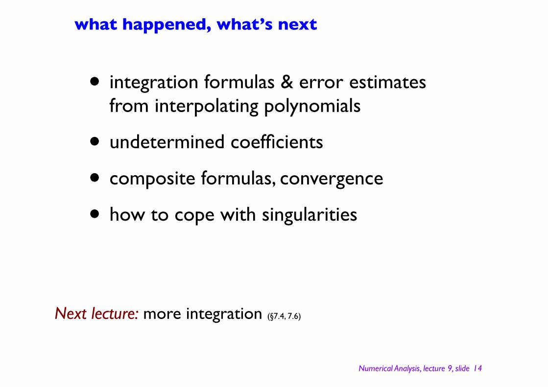
The convergence is slower when the integrand is not smooth enough (p. 176-178)

h Simpson error3/16 6.5104e-043/32 -8.1380e-053/64 1.0173e-05

x x dx = 73!1

2

"examplediscontinuity in f ′′ !

"#

only O(h3)

arctan xx

= x1 2 !13x3 2 +!

!"#

only O(h1.5 )

example (p.176)

singularity in f′ arctan xx

dx0

0.64

! " 0.3239463

0 0.640

0.8

h Simpson error

0.08 -1.84 !10-3

0.04 -6.49 !10-4

0.02 -2.30 !10-4


A change of variables can make the integrand smoother (p. 177-178)

arctan xx

dx0

0.64

! =t= x! 2arctan t2 dt

0

0.64

!

h Simpson error

0.1 -6.27 !10-6

0.05 -3.85 !10-7

0.025 -2.40 !10-8

!"#

O(h4 )

0 0.80

1

2arctan t2 = 2t2 + 2

3t6 +!

other tricks:• integration by parts (p. 178)

• subtracting the singularity (p. 178)

• series


Termwise integration of a seriesnear the singularity (p. 178-179)

1. split off the singularity

x!1 2 arctan xdx0

0.64

" = x!1 2 arctan xdx0

#

" + x!1 2 arctan xdx#

0.64

"regular

! "### $###

3. choose ε so that |E| ≤ tol; compute the regular part using e.g. Simpson

Three stages:

2. integrate a few terms of the series, find the error

x!1 2 arctan xdx

0

"

# = x1 2 !13x5 2 +!$

%&'()dx

0

"

# =23" 3 2 + E, E *

221

" 7 2


what happened, what’s next

• integration formulas & error estimates from interpolating polynomials

• undetermined coefficients

• composite formulas, convergence

• how to cope with singularities

Next lecture: more integration (§7.4, 7.6)

Numerical Analysis, lecture 10: Integration II

(textbook sections 7.4-6)

• Romberg integration

• adaptive methods

• how to tame difficult integrals

0 1

1


A numerical integration formula is a weighted sum of function values (p. 171-172)

f (x) dxa

b! " Ai f (xi )

i=0

n

#

composite trapezoidal rulea b

f (x) dxa

b! = h 1

2 f (a) + f (a + h) +!+ f (b " h) + 12 f (b)( )

T (h)" #$$$$$$$$ %$$$$$$$$

"b " a12

h2 ##f ($)

T (h) =12 T (2h) + h f (a + h) + f (a + 3h)!+ f (b ! h)( )

recursive panel-halving

Compute T (1), T (12 ), T ( 1

4 ), T (18 ) for 1

1+ xdx

0

1

!example


The composite trap rule’s error formulais a series of even powers of h (p. 171)

The composite trapezoidal rule's error is

f (x) dxa

b! " T =

h2

12#f (a) " #f (b)( ) + (b " a) h

4

720f (4)($)

theorem

more generally: (Euler-Maclaurin summation formula)

f (x) dxa

b! = T +

1(2k)!

B2kh2k f (2k"1)(a) " f (2k"1)(b)( ) "

k=1

m"1

# b " a(2m)!

B2mh2m f (2m)($)

…consequently, the composite trap rule is very accurate for periodic integrands


Extrapolation uses 2 low-order approximationsto compute a high-order approximation (p. 171-172)

note: • T (h) can be computed using recursive panel-halving formula

•T (h) ! T (2h)

3 is an error estimate for T2(h)

example (p. 172)

11+ x

dx0

1

!

h T1(h) ! 3 T2(h)1 0.750000

1 2 0.708333 "13889 #10"6 0.694444

1 4 0.697024 "3770 #10"6 0.693254

1 8 0.694122 "967 #10"6 0.693155

I = T (h) + h2

12!f (a) " !f (b)( ) +O(h4 )

I = T (2h) + (2h)2

12!f (a) " !f (b)( ) +O(h4 )

!"#

$#I = T (h) + T (h) % T (2h)

22 %1T2(h)

! "### $###+O(h4 )


Apply extrapolation recursively to obtain higher-order approximations (p. 171-172)

T2 = T (h) +T (h) ! T (2h)

22 !1

T3 = T2(h) +T2(h) ! T2(2h)

24 !1

T4 = T3(h) +T3(h) ! T3(2h)

26 !1!

h T1(h) ! 3 T2(h) ! 15 T3(h) ! 63 T4 (h)1 0.750000

1 2 0.708333 "13889 #10"6 0.694444

1 4 0.697024 "3770 #10"6 0.693254 "79 #10"6 0.693175

1 8 0.694122 "967 #10"6 0.693155 "7 #10"6 0.693148 0 0.693148

example (p.172)

O(h4 )

O(h6 )

O(h8 )


The Romberg table computed in Matlab (p. 173)

>> f = @(x) 1./(1+x);>> romberg(f,0,1)

ans = 0.75000000000000 NaN NaN NaN 0.70833333333333 0.69444444444444 NaN NaN 0.69702380952381 0.69325396825397 0.69317460317460 NaN 0.69412185037185 0.69315453065453 0.69314790148123 0.69314747764483

function R = romberg(f,a,b,q)if nargin<4, q = 2; end R = NaN(q+2,q+2);h = b-a; m = 1;R(1,1) = h*(f(a)+f(b))/2;for i = 2:q+2 h = h/2; m = 2*m; R(i,1) = R(i-1,1)/2 + h*sum(f(a+h*(1:2:m))); for j = 1:i-1 R(i,j+1) = R(i,j) + (R(i,j) - R(i-1,j))/(2^(2*j)-1); endend


Adaptive quadrature recursively subdivides intervals where error is largest (p. 180-181)

Divide & conquer

f (x) dxa

b

! " adpi(a,b, tol, S[a,b])

function adpi(a,b, tol, I1)I2 = S

[a, a+b2

] + S

[a+b2

, b]

E =I2 ! I1

15if E " tol return I2

else

return adpi(a, a + b2

, tol2

,S[a, a+b

2]) + adpi( a + b

2,b, tol

2,S

[a+b2

, b])

Simpson’s rule value of integral


An adaptive quadrature Matlab program (p. 181-182)

function I = adaptint(f,a,b,tol)ff = f([a,(a+b)/2,b]);I1 = (b-a)*[1 4 1]*ff(:)/6;I = adpi(f,a,b,tol,ff,I1); function I = adpi(f,a,b,tol,ff,I1)h = (b-a)/2; m = (a+b)/2;fm = f([(a+m)/2 (m+b)/2]);IL = h*[1 4 1]*[ff(1);fm(1);ff(2)]/6;IR = h*[1 4 1]*[ff(2);fm(2);ff(3)]/6;I2 = IL + IR;I = I2 + (I2-I1)/15;if abs(I-I2) > tol IL = adpi(f,a,m,tol/2,[ff(1) fm(1) ff(2)],IL); IR = adpi(f,m,b,tol/2,[ff(2) fm(2) ff(3)],IR); I = IL + IR;end

>> f = @(x) x+(0.2)./(1000*(x-0.3).^2+1);>> adaptint(f,0,1,1e-6)

ans = 0.51892

0 1

1

>> quad(f,0,1,1e-6)

ans = 0.51892


Trapezoidal & Simpson rules can’t be usedif integrand is infinite at an endpoint

arctan xx3 2

dx0

0.64

! " 1.56129860 0.640

8

example (p. 179)

f (x) dx0

0.64! = h 1

2 f (0)"! + f (0 + h) +"+ f (0.64 # h) + 1

2 f (0.64)$

%&&

'

())

arctan xx3/2

= x!1 2 !13x1 2 +!


The convergence is slower when the integrand is not smooth enough (p. 176-178)

arctan xx

= x1 2 !13x3 2 +!

!"#

only O(h1.5 )

example (p.176) singularity in f′arctan x

xdx

0

0.64

! " 0.3239463

0 0.640

0.8

h Simpson error

0.08 -1.84 !10-3

0.04 -6.49 !10-4

0.02 -2.30 !10-4


A change of variables can make the integrand smoother (p. 177-178)

arctan xx

dx0

0.64

! =t= x! 2arctan t2 dt

0

0.64

!

h Simpson error

0.1 -6.27 !10-6

0.05 -3.85 !10-7

0.025 -2.40 !10-8

!"#

O(h4 )

0 0.80

1

2arctan t2 = 2t2 + 2

3t6 +!

other tricks:• integration by parts (p. 178)

• subtracting the singularity (p. 178)

• series


Termwise integration of a seriesnear the singularity (p. 178-179)

1. split off the singularity

x!1 2 arctan xdx0

0.64

" = x!1 2 arctan xdx0

#

" + x!1 2 arctan xdx#

0.64

"regular

! "### $###

3. choose ε so that |E| ≤ tol; compute the regular part using e.g. Simpson

Three stages:

2. integrate a few terms of the series, find the error

x!1 2 arctan xdx

0

"

# = x1 2 !13x5 2 +!$

%&'()dx

0

"

# =23" 3 2 + E, E *

221

" 7 2


There are several ways of dealing with an infinite integration interval (p. 179)

cutting off the tail

e!x2

0

"

# dx = e!x2

0

a

# dx + E

E = e!x2

a

"

# dx $ 1a

xe!x2

a

"

# dx = 12a

e!a2

>> f = @(x) exp(-x.^2);>> adaptint(f,0,4,1e-6)

ans = 0.88623

>> f = @(x) exp(-(-log(t)).^2)./t;>> adaptint(f,eps,1,1e-6)

ans = 0.88623

change of variables

e!x2

0

"

# dx

0 10

1

0 40

1

0 10

1

0 40

1

=

t=e! x!

1te!(! log t )

2dt

0

1

"


what happened, what’s next

• Trapezoid rule’s error formula has even powers of h

• Romberg method recursively combines different h approximations to obtain a higher order

• Adaptive quadrature based on local error estimates

• coping with singularities: change of variable, series

• Two ways of handling infinite interval

Next lecture: approximation (§9.1-3)

Documents

Numerical Analysis, lecture 9: Integrationbutler.cc.tut.fi/~piche/numa/lecture0910.pdf · Numerical Analysis, lecture 9, slide ! 6 The method of undetermined coefﬁcients is another