Embed Size (px)
Citation preview

1
Numerical Analysis
Lecture Notes
By
Dr. Maan A. Rasheed
2018

2
Contains
Chapter 1: Introduction
Types and sources of errors
Chapter2: Numerical solutions for nonlinear equations
Bisection
Newton-Raphson
Fixed point Method
Chapter 3: Numerical solutions of linear systems
Direct methods
Gauss Elimination Method
Gauss-Jordan Method
LU Method
Indirect Methods
Jacobi Method
Gauss-Sidel Method
Chapter 4: Interpolation, Extrapolation and numerical and differentiation
Finite difference operators
Newton’s finite difference formulas
Forward formula
Backward formula
Centre formula
Chapter 5: Numerical integration
Trapezoidal method
Composite Trapezoidal method
Simpson Method
Composite Simpson method

3
Chapter 6:Numerical Solutions of First Order Ordinary Differential
Equations
Euler Method
Modified Euler Method
Runge-Kutta Method of order2
Runge-Kutta Method of order4
Recommend Books
1-Applied Numerical Analysis,
by R. L. Burden, J. D. Faires, Brooks/Cole, Cengage Learning, USA, 2015.
2- An Introduction to Programming and Numerical Methods in MATLAB,
by S.R. Otto & J.P. Denier, Springer-Verlag London Limited, 2005.

4
Chapter One
Introduction
Numerical Analysis is a field of mathematics that concerned with the study of
approximate solutions of mathematical problems, where it is difficult or impossible
to find the exact solutions for these problems.
For instance, we can’t find the exact value of the following integral
, by using known integration methods, ∫
while we can find an approximate value for this integral, using numerical
methods.
The other example, if we aim to find the solution of a linear system
where , when n is too large , it so difficult to find the exact solutions
for this system by hand using known methods, so in this case, it is easier to think
about how to find the approximate solution using a suitable algorithm and
computer programs.
The importance of Numerical Analysis
To interpret any real phenomena, we need to formulate it, in a mathematical
form. To give a realistic meaning for these phenomena we have to choose
complicated mathematical models, but the problem is, it so difficult to find explicit
formulas to find the exact solutions for these complicated models. Therefore, it
might be better to find the numerical solutions for complicated form rather than
finding the exact solutions for easier forms that can’t describe these phenomena in
realistic way.
The nature of Numerical analysis
Since for any numerical Algorithm (the steps of the numerical method), we have
lots of mathematical calculations, we need to choose a suitable computer language
such as Matlab or Mable and write the algorithm processes in programing steps.

5
In fact, the accuracy of numerical solutions, for any problem, is controlled by three
criteria:
1- The type of algorithm,
2- The type of computer language and programs,
3- The advancement of the computers which are used.
Types and sources of Errors
When we compute the numerical solutions of mathematical model that we use to
describe a real phenomenon, we get some errors; therefore we should study the
types and sources of these errors.
We can point out the most important types and sources of these errors as follows:
1- Rounding errors: this type of errors can be got, because of the rounding of
numbers in computer programming languages.
Example:- 5.99…9 round to 6, and 3.0001 round to 3.
2- Truncation Errors: Since most of numerical algorithms depend on writing
the functions as infinite series, and since it’s impossible to take more than
few terms of these series when we formulate the algorithm, therefore, we get
errors, called truncation errors.
Example :-
( )
If we compute ( ) with taking 4 terms, we get more errors than with taking 10
terms.
3-Total errors:- Since any numerical algorithm is about iterative presses, the
solution in step depends on the solution in step ( ). Therefore, for larger
number of steps we get more errors, and those errors are the total of all previous
types of errors.
Let is the approximate value of , there are two methods can be used to
measure the errors:-

6
1- Absolute Error:-
2- Relative error:-
Example:- Let . Find the Absolute and Relative
errors
Solution
,
Remark: Clearly,
Questions
Q1:
i- What is numerical analysis concerned with?, and what is the
importance of studying this subject ?,
ii- What are the most important types of errors that arise from using a
numerical method to compute the numerical solution of a mathematical
problem?
iii- What are the criteria that control the accurse of numerical solutions?
Q2: Let be the absolute and relative errors, respectively, in an
approximate value of . Show that , if .

7
Chapter 2
Numerical Solutions for Nonlinear Equations
There are lots of real problems, can be solved by mathematical forms, and these
forms has nonlinear equations. Mostly, it is difficult to calculate the exact solutions
for these equations; therefore, we study some numerical methods in order to be
able to find the approximate solutions for these equations.
Examples
( ) , ( ) nonlinear equations for one variable
( ) ( ) ( )
nonlinear equations for two variables
Roots of nonlinear equations of one variable
Finding the solution for a nonlinear equation of one variable, ( ) means,
finding a value , such that ( ) where is called the root of ( )
Remark: Some equations have more than one root.
Example:
1- ( ) ( )( )
Since ( ) ( ) , it follows that both of are roots for the
nonlinear equation above.
2- ( ) we see that , are roots for
3- ( ) ( ) , we see that , is the double root for .
The approximate roots for non-linear equations
In order to ensure that, there exist a root for the equation ( ) on the
interval , - we have to make sure that ( ) ( ) see the following figure:

8
( )
( )
Remark:- Let be the exact root of the equation ( ) , and is a
subsequence of approximate roots, that can be got from using a numerical method,
for large the following condition has to satisfy:
( ) or
Next, we study some known numerical algorithms those can be used to find the
approximate solutions (roots) for non-linear equations, which are Bisection
algorithm, Newton–Raphson algorithm and fixed point algorithm.
Bisection Algorithm
Let , -
i.e. is continuous function on the closed interval , -
Assume that the condition ( ) ( ) is satisfied, we follow the following
steps:
1- We bisect the space as follows:
or
2- If ( ) , it follows that is the exact root, otherwise check the sign of
( ) , if ( ) ( ) then the exact root belong to , -, and we set
, and then we repeat the same steps.

9
While, if ( ) ( ) then the exact root belong to , -, and we set
, , and then we repeat the same steps.
3- We continue iteratively, until we get the following condition is satisfied
( ) or
or
+ + _ _
( ) ( ) ( ) ( )
] ] [ [ [
Remarks:
1- From the iterative processes of Bisection algorithm, we get a sequence of
closed intervals , -, and for i<j, the length of , - is shorter than
the length of [ , ] and . Therefore, according to known real analysis
theorems, the intersection of all these intervals contains only one point, which is
the exact root of ( ) .
2- From the iterative processes of Bisection algorithm, we get a sequence of
approximate roots, { } for the nonlinear equation ( ) , which is convergent
to the exact root i.e. * + → →
10
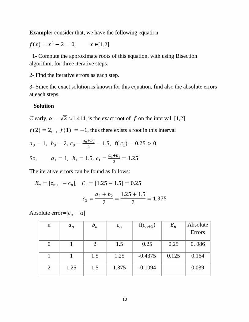
Example: consider that, we have the following equation
( ) [1,2],
1- Compute the approximate roots of this equation, with using Bisection
algorithm, for three iterative steps.
2- Find the iterative errors as each step.
3- Since the exact solution is known for this equation, find also the absolute errors
at each steps.
Solution
Clearly, √ 1.414, is the exact root of on the interval [1,2]
( ) ( ) , thus there exists a root in this interval
, ( )
So,
The iterative errors can be found as follows:
Absolute error |
Absolute
Errors
f( ) n
0. 086 0.25 0.25 1.5 2 1 0
0.164 0.125 -0.4375 1.25 1.5 1 1
0.039 -0.1094 1.375 1.5 1.25 2

11
The iterative error, - |=1.25, clearly, it is, still too large, so we have to
continue in the iterative processes until we get the convergent condition,
or
Matlab Code for Bisection Method
Write the Matlab code which can be used to find the approximate root of ( )
, -, with considering
1- a=input('a=');
2- b=input('b=');
3- x=sym('x');
4- f=x^2+x-1;;
5- fa=subs(f,x,a);
6- fb=subs(f,x,b);
7- k=0;
8- if fa*fb>0
9- fprintf('the function f(x) has no root')
10- break;
11- else
12- while abs(b-a)>0.0001
13- c=(a+b)/2;
14- fc=subs(f,x,c);
15- if fc==0
16- fprintf('the exact root=%f',c);
17- fprintf('the number of iteration=%d',k);
18- break;
19- end
20- if fa*fc>0
21 a=c; fa=fc;
22- else
23- b=c; fb=fc;
24- end
25- k=k+1;

12
26- end
27- fprintf('the approximate root=%f',c);
28- fprintf('the number of iteration=%d',k)
29- end
a=0
b=1
Answer: the approximate root=0.617981
the number of iteration=14
H.w:- Find the approximate roots of the following equation:
( ) on the closed interval [0,3].
Method Raphson-Newton
This algorithm can be used to find the approximate toots for the equation ( )
when it easy to find the derivative,
Deriving the Newton-Raphson’s formula:
Let , -
i.e. , -
let * +, is a sequence of approximate roots for , such that:
( )
where, ( )
Use Taylor expansion for , around , we get
( ) ( ) ( ) ( )
( )
( )
substitute
13
( ) ( ) ( ) ( ) ( )
( )
( )
( )
( )
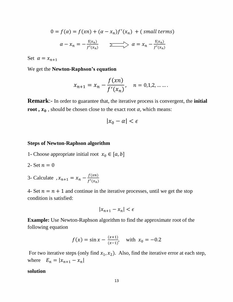
Set
We get the Newton-Raphson’s equation
( )
( )
Remark:- In order to guarantee that, the iterative process is convergent, the initial
root , , should be chosen close to the exact root which means:
Steps of Newton-Raphson algorithm
1- Choose appropriate initial root , -
2- Set
3- Calculate ( )
( )
4- Set and continue in the iterative processes, until we get the stop
condition is satisfied:
Example: Use Newton-Raphson algorithm to find the approximate root of the
following equation
( ) ( )
( ) with
For two iterative steps (only find ) Also, find the iterative error at each step,
where
solution

14
( ) ( ) ( )
( )
( )
( ) ( ) ( )
( ) ( )
( ) ( )
( )
Thus
( )
( ) ( )
( )
( )
( )
( ) ( )
By the same way, we can find
We continue, iteratively, until we get the stop condition is satisfied:
( ) ( ) N
0.1976 -0.2000 0
0.0225 0649.1 1
0.0003 -0.4201 2
0.0001 169419- 3
169410- 4
Matlab Code for Newton-Raphson algorithm

15
We can write a Matlab code to find the approximate root of the last example using
N.R. algorithm, as follows:
1- x0=input('x0=');
2- x=sym('x');
3- f=sin(x)-((x+1)/(x-1));
4- g=diff(f);
5- fx0=subs(f,x,x0)
6- gx0=subs(g,x,x0)
7- k=0;
8- x1=x0-(fx0/gx0)
9- fx1=subs(f,x,x1);
10- while abs(fx0/gx0)>eps;
11- fx1=subs(f,x,x1);
12- if fx1==0
13- fprintf('The exact root=%f',x1);
14- break;
15- else
16- x0=x1;
17- end
18- k=k+1;
19- fx0=subs(f,x,x0)
20- gx0=subs(g,x,x0)
21- x1=x0-(fx0/gx0)
22- end
23- fprintf('the approximate root=%f',x1);
24- fprintf('the number of iteration=%d',k);
Answer: the approximate root= - 0.420362
the number of iteration=4

16
Fixed Point Algorithm
This method depends on the concept of fixed points for one variable functions
Definition :- The point which belongs to the domain of the function is called
a fixed point for , iff ( )
We can give the idea of this algorithm as follows:
We write the function , where ( ) as follows:
( ) ( )
such that , is a root for ,thus ( )
which means that, a fixed point for g, that is
( ) → ( )
Therefore, the problem becomes, we have to look for the fixed point of rather
than, looking for the root of .
Fixed point Theorem:-
Let , - ( ) , - , -
Then g has a fixed point on [a,b], moreover, if exists on (a,b), such that
| (x)|
Then g has a unique fixed point , , -.
Remark :- when we choose a certain form for g , we have to make sure that
( ) ( )
This condition can guarantee the convergence for the algorithm.

17
Fixed point algorithm steps
1-Choose the initial root
2-Choose a form for the function g, such that
( ) ( )
3- Set ( ) ( )
4- We continue in the iterative process until we get:
Example: - Find the approximate root of the following equation
( ) , on the interval [1, 3.5], with considering that
, for two iterative steps (find only )
Solution
Let us choose two forms for g as follows:
( )
( )
( )
……..(2)
( )
( )
( )
It is clear that, ( )| ( )
while | ( )|
Therefore, we ignore and choose the convergent form
Next, we find ,……

18
( )
. /
( )
. /
We continue, with n=3,4,…..until 29.
Where and
H.W. For last example find the iterative errors for three steps.
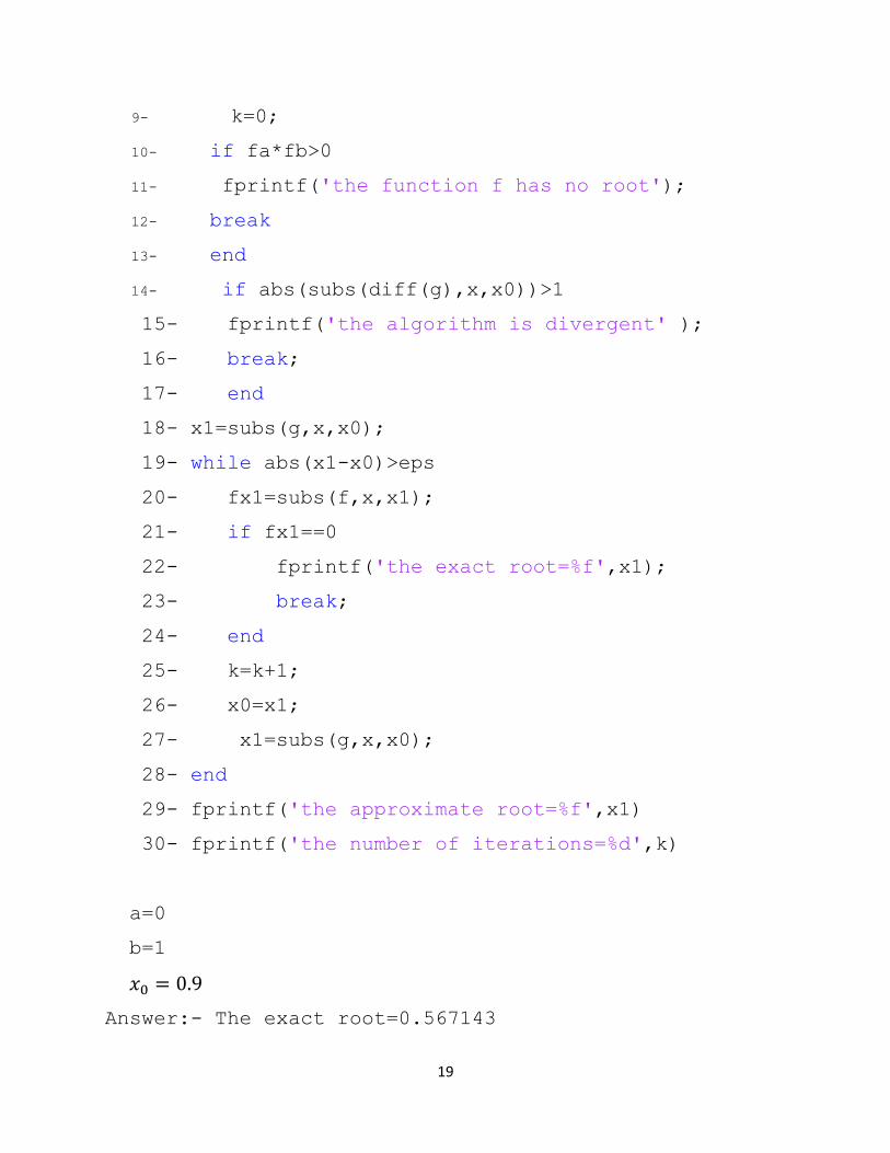
Example 2, write the Matlab code that can be used to find the approximate root of
the following equation
( ) , on the interval [0, 1], consider
Before to write the grogram let us study the possible forms for g
( )
( )
( ) ( )
Since ( )
( )
( )
Therefore, we choose the first for
1- a=input('a=');
2- b=input('b=');
3- x0=input('x0=');
4- x=sym('x');
5- f=x-exp(-x);
6- g=exp(-x);
7- fa=subs(f,x,a);
8- fb=subs(f,x,b);
19
9- k=0;
10- if fa*fb>0
11- fprintf('the function f has no root');
12- break
13- end
14- if abs(subs(diff(g),x,x0))>1
15- fprintf('the algorithm is divergent' );
16- break;
17- end
18- x1=subs(g,x,x0);
19- while abs(x1-x0)>eps
20- fx1=subs(f,x,x1);
21- if fx1==0
22- fprintf('the exact root=%f',x1);
23- break;
24- end
25- k=k+1;
26- x0=x1;
27- x1=subs(g,x,x0);
28- end
29- fprintf('the approximate root=%f',x1)
30- fprintf('the number of iterations=%d',k)
a=0
b=1
Answer:- The exact root=0.567143

20
The number of iterations=63
H.W. :- Find the approximate root of the following equation
( ) , on the interval [0.25, 0.75], consider
Exercises
Q1:- Find the approximate roots of the following equation
( ) on [0,1], by using fixed point method (for three
iterative steps), and find the iterative errors at each step. What is the stop
condition?
Q2:- Find the approximate value of √
by using Bisection Algorithm (for three
iterative steps) and find the absolute errors at each step.
Hint: consider ( ) √
Q3:- Use Newton-Raphson algorithm to find the approximate roots of the
following equation
( )
( ) , for three iterative steps,
and find the absolute errors at each step.

21
Chapter 3
The Numerical Solutions of Linear Systems
It is well known from the linear algebra that, that there are many methods used to
find the exact solutions of linear systems, where ,
such as Gauss elimination or, Gauss-Gordan, or Kramer’s method. But using these
methods becomes so difficult when the dimension , of the matrix , is large.
Therefore, we need to compute the solutions numerically by using computers.
In general, there are two types of numerical methods, which can be used to find the
numerical solutions of linear systems: direct methods and indirect methods.
Before starting to study these methods, let’s revision some equivalent algebraic
facts of the linear system:
1-The homogenous system , has only zero solution, iff , which
means is nonsingular matrix.
2-The linear system , has a unique solution , iff , which means
A is nonsingular matrix.
From above, before to think about finding a numerical solution of a linear
system, we need make sure that the exact solution exists, which means we
should check whether or A is nonsingular.
Direct methods
These methods can be convergent very fast, but when the dimension of A is large,
it is not recommended to use these methods because, we need to compute lots of
mathematical operations, which means, the errors become bigger.
Next, we will study some of direct methods.
Gauss Elimination Algorithm
The idea of this method, is to convert A in the linear system , to upper U or
lower matrix L. Thus, we get a lower or upper triangular system:

22
It is clear that, for solving lower triangular system we use Forward substitutions
and for solving upper triangular system we use Backward substitutions.
In fact, solving lower (upper) triangular system is easier than solving the original
system.
Steps of Gauss elimination algorithm:
1- Write the system , in the matrix form [A: b].
2- Convert [A: b] to appear triangular form , - or lower triangular from
, -
3-Solve the lower (upper) triangular system, ( ) by using
forward (backward) substitutions.
Example:- Solve the following linear system by using Gauss algorithm
Solution
Firstly, we write the system in matrix form , -, as follows
0
1
( )/5 , -4( /5)+
[
]
Thus, we get the following upper triangular system
( )
( )
Finally, we solve the last system by using the backward substitutions, to get

23
( ) ( )
Thus, the solution is
=( ) x=(
)
H.W. In the last example, try to change the system , to a lower
triangular system and find its solution by using the forward substitutions.
Matlab Code for Gauss Method
Write a Matlab program, which can be used to find the solution of the
following system by using Gauss method with back ward substitutions
A=[4,-9,2;2,-4,6;1,-1,3];
b=[5;3;4];
n=3;
for k=1:n-1;
for i=k+1:n
m(i,k)=A(i,k)/A(k,k);
for j=k:n
A(i,j)=A(i,j)-m(i,k)*A(k,j);
end
b(i)=b(i)-m(i,k)*b(k);
end
end
x(n)=b(n)/A(n,n);
for i=n-1:-1:1
s=0;
for j=i+1:n
s=s+A(i,j)*x(j);
end
x(i)=(b(i)-s)/A(i,i);
end

24
disp(x);
6.9500 2.5000 -0.1500
Gauss- Gordan algorithm
This algorithm is considered, as a modified to the Gauss elimination
algorithm. We convert the linear system, , to , where
is the identity matrix of order . Thus to solve the last system we use the
direct substitutions.
Ax=b
Steps of Gauss- Gordan algorithm
1- Write the system , in the matrix form [A: b].
2- Do some mathematical operations to convert [A: b] to the diagonal form
, -.
3- Find by solving the system using direct substitutions.
Example :- Find the solution of the following system, by using Gauss-Gordan
Method
Solution
Firstly, we write the system in matrix form , -, as follows:
0
1……(1) -2( )+ 0
1 ……..(2)
( ) [
]……(3)
-2( )+ [
]……(4)

25
Thus, we get
0 1=[
]
: LU Algorithm
This method is called by LU, because the matrix in the linear system ,
decomposes into the multiplication of two matrices : lower L and upper U, and this
decomposition works for any vector b, which means
Thus, we get lower triangular and upper triangular systems.
In order to get the solution of the system , we need to solve these two
systems.
Steps of LU Method
1- Decompose , in the form where U is an upper matrix and L is a lower
matrix.
2- Set Ux=y, which leads to Ly=b
3-Solve first the lower triangular system, Ly=b, using the forward substitutions to
get y, and then solve the lower triangular system, Ux=y, using the backward
substitutions to get x .
Remarks:-
1-This method can be considered better than Gauss and Gauss-Gordan methods
and that because the decomposition of the matrix works for any vector , while
in Gauss and Gauss - Gordan, the mathematical operations, which we have to do
on [A:b], should be redone again when we choose another vector .
2-In fact, not any matrix A can be decomposed to LU, unless the following
condition (The diagonal control condition), is satisfied.
∑
, i=1,2,..n
Example:- Can we decompose the matrix to ?, where

26
A=(
)
Solution
Since, A satisfies the diagonal control condition
Therefore, it follows that can be decomposed to LU.
The following example shows how to use LU algorithm to solve a linear
system.
Example:- Use LU Algorithm to find the solution of the following system.
Solution
Set
A=0
1 =0
1 0
1
L U
( )( )
It follows that
0
1 = u , L=0
1
Set
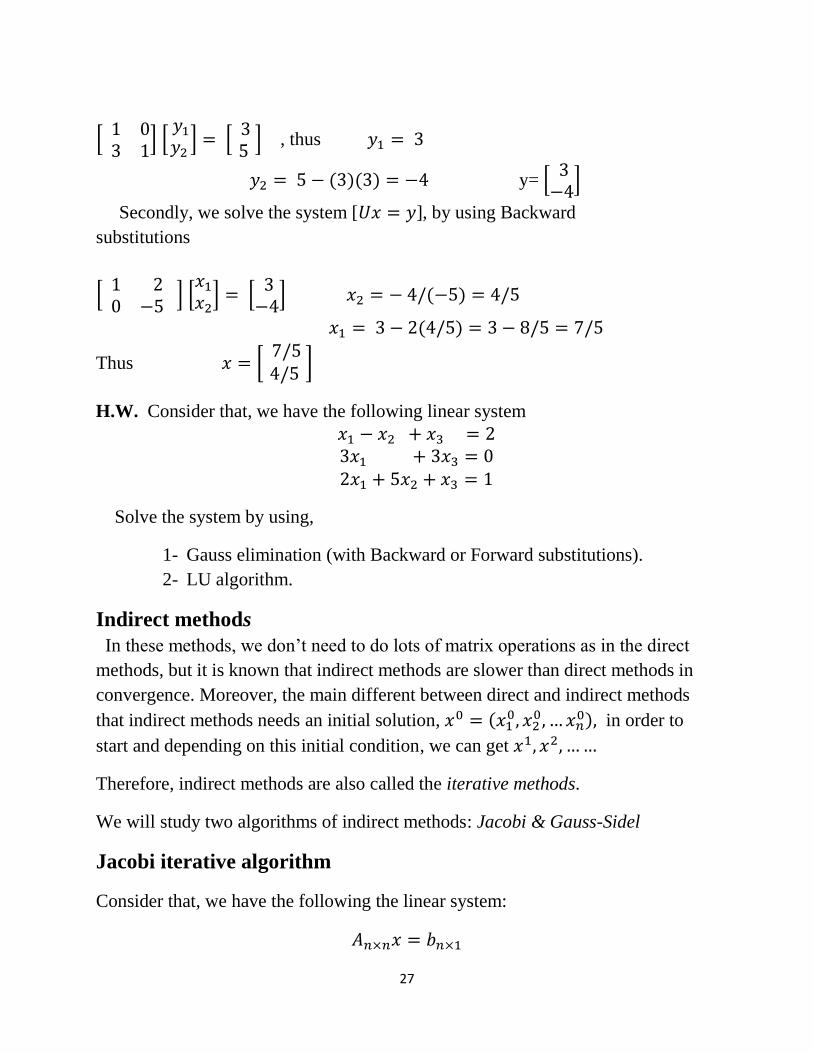
We need to solve first the system , - by using Forward substitutions
27
0
1 0 1 0
1 , thus
( )( ) y= 0 1
Secondly, we solve the system [ ], by using Backward
substitutions
0
1 0 1 0
1 ( )
( )
Thus [
]
H.W. Consider that, we have the following linear system
Solve the system by using,
1- Gauss elimination (with Backward or Forward substitutions).
2- LU algorithm.
Indirect methods
In these methods, we don’t need to do lots of matrix operations as in the direct
methods, but it is known that indirect methods are slower than direct methods in
convergence. Moreover, the main different between direct and indirect methods
that indirect methods needs an initial solution, (
) in order to
start and depending on this initial condition, we can get
Therefore, indirect methods are also called the iterative methods.
We will study two algorithms of indirect methods: Jacobi & Gauss-Sidel
Jacobi iterative algorithm
Consider that, we have the following the linear system:

28
which can be written as follows:
+ +……….+ =
+ +………….+ =
+ ………..+
where
Remarks:
1- In case of we replace the equation number i, with
another equation in order to get
2- On the other hand, in order to get faster convergence, we should make sure that,
The diagonal control condition is satisfied
| |≥∑
In case of this condition is not satisfied, we can also switch places between the
equations, until we get this condition is satisfied.
Steps of Jacobi algorithm
1-Make sure that the system has a unique solution, .
2-Choose the initial solution (
)
3-Make sure that ∑
and in case of one of these condition is not satisfied, switch places of the equations,
until we get the two conditions are satisfied.
4- Write the system in iterative form: ( ∑
) for

29
5-Compute the solution iterative iteratively, ( for ), until we get the
following the stop condition is satisfied:
‖ ( ) ( )‖ where
‖ ( ) ( )‖
|
|
Example:- Use Jacobi algorithm to solve the following linear system, for
two iterative step and find the iterative error at each step.
Note: The exact solution for this system is x=( 1; 2; 3)
Solution
Since we need to switch the places of equation 2 and 3:
It is clear that, the last system satisfies the diagonal control condition.
We can rewrite the last system as follows:
=
+
=4 -
-
We write the system in the iterative form as follows:
=

30
k=0,1,…….
Let =( ,
, )=(0.8, 1.8, 2.8)
Set k=0
( )
=
-
( ) -
( ) =
( )
=
+
( ) =
( )
= 4 -
(0.8) -
( ) =
( ) ( )
* +
set , by using the same way obtain:
( )
( )
( ) ,
( )
( ) ,
( )
( )
( ) 2.95
( ) ( )
* +
We continue iteratively, until the convergent condition can be satisfied:
|| ( ) - ||<
Gauss – Sidel algorithm
The main difference between this method and Jacobi method, is for any iterative
step ,k, the new approximate values of the , are used directly, to

31
compute the approximate values of , while in Jacobi we don’t use the new
approximate values until, we consider the next iterative step, .
Remark: The steps of Gauss-Sidel algorithm are the same as the step of Jacobi
method expect for in step (4), we use the Gauss-Sidel iterative system:
( ∑
∑
)
for
Example:- Use Gauss-Sidel algorithm to find the approximate solution to
the following system for two iterative steps, with =(0.8, 1.8, 2.8), and find
the iterative errors at each step.
It is clear that, the last system satisfies the diagonal control
condition.
We can rewrite the last system as follows:
=
+
=4 -
-
We write the system in the iterative form as follows
=
-
-
=
+
= 4-
-

32
Set k=0, we get
( )
=
-
( ) -
( ) =
( )
=
+
( ) =
( )
= 4 -
(1.15) -
( ) =
( ) ( )
* +
Set k=1, we can, in the same way, compute
( )
=
-
( ) -
( ) =0.9859
( )
=
+
(0.9859) =1.993
= 4 –
( ) –
( )
( ) ( )
* +
We continue iteratively, until the convergent condition can be satisfied:
|| ( ) - ||< or ‖ ( )‖
Remark: From last example, we see that, the approximate results that we get by
using Gauss-Sidel are more accurate and closer to the exact solution, compared
with the results that we got by using Jacobi method. Moreover, for ,the
iterative errors those arise from using Gauss-Sidel method are less than the
iterative errors those arise from using Gauss-Sidel. Which means Gauss-Sidel
method is faster than Jacobi method in convergence.

33
Matlab Code
Write a matlab program, which can be used to find the approximate solution
of the following system by using
1- Jacobi Method
2-Gauss-Sidel
with ( )
Jacobi
A=[9,-4,2;2,-4,1;1,-1,3];
b=[5;3;4];
n=3;
x0=[0;0;0];
r=norm(b-A*x0);
k=0;
while r> 0.01
k=k+1;
for i=1:n
s=0;
for j=1:i-1
s=s+A(i,j)*x0(j);
end
for j=i+1:n
s=s+A(i,j)*x0(j);
end
x(i)=(b(i)-s)/A(i,i);
end
x0=x' ;
r=norm(b-A*x0);
end
disp(x);
disp(k);
34
0.1205 -0.4005 1.1605 k=19
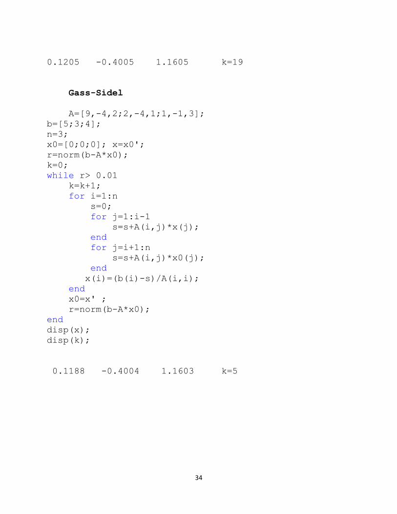
Gass-Sidel
A=[9,-4,2;2,-4,1;1,-1,3];
b=[5;3;4];
n=3;
x0=[0;0;0]; x=x0';
r=norm(b-A*x0);
k=0;
while r> 0.01
k=k+1;
for i=1:n
s=0;
for j=1:i-1
s=s+A(i,j)*x(j);
end
for j=i+1:n
s=s+A(i,j)*x0(j);
end
x(i)=(b(i)-s)/A(i,i);
end
x0=x' ;
r=norm(b-A*x0);
end
disp(x);
disp(k);
0.1188 -0.4004 1.1603 k=5
35
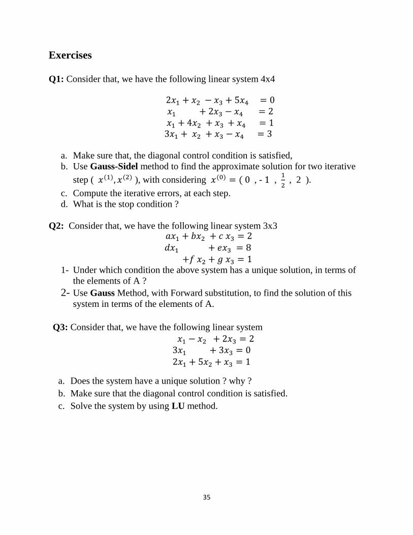
Exercises
Q1: Consider that, we have the following linear system 4x4
a. Make sure that, the diagonal control condition is satisfied,
b. Use Gauss-Sidel method to find the approximate solution for two iterative
step ( ( ) ( ) ), with considering ( ) ( , - ,
, 2 ).
c. Compute the iterative errors, at each step.
d. What is the stop condition ?
Q2: Consider that, we have the following linear system 3x3
1- Under which condition the above system has a unique solution, in terms of
the elements of A ?
2- Use Gauss Method, with Forward substitution, to find the solution of this
system in terms of the elements of A.
Q3: Consider that, we have the following linear system
a. Does the system have a unique solution ? why ?
b. Make sure that the diagonal control condition is satisfied.
c. Solve the system by using LU method.

36
Chapter 4
Interpolation,Extrapolation & Numerical Differentiations
Sometimes, we need to estimate an unknown value depending on known values
(Data base), for instance, consider that, the numbers of people who have lived in Iraq is
known, for the years 57, 67, 77,87, 97,2007, 2017, if we would like to estimate the
number of Iraq’s people in the year 75, this operation is called the interpolation,
because the number 75 belongs to the interval [37, 87], while , if we would like to
estimate the number of Iraqi people in the year 2018, this operation is called the
extrapolation, because the number 2018 does not belong to the range of the data base.
Mathematical problems of interpolation and extrapolation
Assume that, we have the following database, where is a continuous function on
[ -
( ) ,
.............. ...........
, or ,
If the aim is to find ( ), where ) , - then this operation is
called the interpolation ,
while, if the aim is to find ( ), where ) , -
then, the operation is called Extrapolation
Next, we will study some finite difference methods that can be used to find the
solutions for interpolation problems, when the distances between the points in the
database are equal.
Finite Difference Operators
The finite difference operators can be classified into three types:

37
Forward , Backward 𝛁 and Center 𝜹.
In order to understand the difference operators, we divide the interval , -, as
follows:
where , is the distance between any two points
Forward difference operator
The Forward difference operator is defined as follows:
( ) ( ) ( )
( ) ( )
( ) ( ( )) ( ( ) ( )) ( ) ( )
( ) ( ) ( ) ( )
By the same way, we can find
Backword difference operator
The Backward difference operator is defined as follows:
( ) ( ) ( )
=
( ) ( )
=
=
=

38
Center difference operator
The centre difference operator is defined as follows:
( ) (
) (
)
(
)
=
=
Newton’s formulas by using (Forward, Backward, Center) Finite
Difference Operators
Consider, we have the following data base:
Where ,
……………
……………
Our aim to find ( ), where ,
If close to the beginning of the database ( ), then we use Newton
Forward formula, which takes the form:
( ) ( )
while, if close to the end of the data base, ( ), then we use
Newton Backward formula, which takes the form:
( ) 𝛻 ( )
𝛻

39
where,
If close to the centre of the database, ( ), then we use Newton centre formula,
which takes the form:
( ) ( )
( )
where ,
Steps of Newton’s formulas:
1- Input the values of ) )
2- Input
3-set
4- If is close to , and set
compute and use Newton’s
forward formula, to find ( ),
If close to , set
, compute and use Newton’s
Backward formula, to find ( ),
If , where set
, compute
and use Newton’s center formula, to find ( ).
Example:- consider the following data base
10 8 6 4 X
20 8 3 1 ( )
Find the approximate value for each of the following:
( ) 3- ( ) 2- 1- ( )

40
Solution
1- Since 4.5 close to the beginning of the data base, we use the forward
Newton formula
( ) ( )
( )
or for simplicity can be also found from the following figure
4 1
6 3
5
8 8
10 20
Thus
( )
( ) .
/ .
/( )
= 1.2188
2- Since the point 9 close to the end of the database ( ), we use the
Backward Newton formula,

41
Set,
( ) ( )
𝛻
𝛻
( )
Or for simplicity 𝛻 can be also found from the following figure
4 1
6 3
5
8 8
𝛻
10 20
Thus ( ) (
)( )
.
/.
/
( )
Finally, since 6.4 close to the middle of the database (between ) , we
use the Center Newton formula
,

42
( ) ( )
( )
( )
( )
For simplicity, can be found from the following figure
4 1
6 3
5
8 8
10 20
Thus
( ) ( )( ) ,( ) -
( ) ( )( )
,( ) -
( )
=3.6320

43
Matlab Codes for Finite Difference Methods
Example: Consider the following database
1.5 1 0.5 0 X
3.25 2 1.25 1 ( )
Write Matlab codes that can be used to find:
Forward ) ( 1- f(0.25)
f(1.25) ( Backward ) 2-
3- f(0.75) ( Centre )
Forward finite difference
x=[0,0.5,1,1.5];
y= [1,1.25,2,3.25];
xp=input('xp=');
h=0.5;
p=(xp-x(1))/h;
Dy0=y(2)-y(1);
D2y0=y(3)-2*y(2)+y(1);
yp=y(1)+p*Dy0+(p*(p-1)/2)*D2y0;
fprintf('f(%f)=%f',xp,yp);
( )
Centre finite difference
x=[0,0.5,1,1.5];

44
y= [1,1.25,2,3.25];
xp=input('xp=');
h=0.5;
p=(xp-x(2))/h;
q=1-p;
S2y1=y(3)-2*y(2)+y(1);
S2y2=y(4)-2*y(3)+y(2);
yp=p*y(3)+p*(p+1)*(p-
1)*S2y2/factorial(3)+q*y(2)+q*(q+1)*(q-
1)*S2y1/factorial(3);
fprintf('f(%f)=%f',xp,yp);
( )
Backward finite difference
x=[0,0.5,1,1.5];
y= [1,1.25,2,3.25];
xp=input('xp=');
h=0.5;
p=(xp-x(4))/h;
By3=y(4)-y(3);
B2y3=y(4)-2*y(3)+y(2);
yp=y(4)+p*By3+(p*(p+1)/2)*B2y3;
fprintf('f(%f)=%f',xp,yp);
xp=1.25
f(1.25)=2.5625

45
Numerical Differentiations
Let , be a differentiable function on , -, and let ) , ], and ( ) -
are
known . So, we have the following database
Let , -
Our aim is to find the derivative of f at ( )
Using Finite difference operators to find derivatives
In case of the distances between the points, ) are equal ,
we can also use Forward, Backward, centre Newton’s formulas, to find
( ) :
Case1: Interpolation Problems
) , - we use Newton’s finite difference formulas as
follows:
Set where
{
}
So,
( )
(
)
( ) (
) ( )
Therefore, Forward, Backward and Center Newton formulas for differentiation take
the forms, respectively:

46
( ) .
/ ( )
(
( )
),
( ) .
/ ( )
(
( )
),
( ) (
) ( )
( )
, ( ) -
Example: Going back the example that we have considered before, find
( ) ( ) ( ) by using (forward, backward, center) Newton formulas.
Solution:-
Since 4.5 close to the beginning of the data base, we use forward formula to find
( )
( )
(
( )
) ,
where
( )
( (
) )
H.W. in the same way we can find ( ) ( ) by using the backward and
center formulas, respectively.
Case2: Computing the Derivatives at the Points of Database
Consider that, we have the following data base:
where
The problem is: how to find the approximate values for ( ) ( )

47
It is well known that,
( ) →
( ) ( )
( )
Thus, for small values of
( ) ( )
( )
Or ( ) → ( ) ( )
( ) ( )
( )
For small values of , we have
( ) ( )
( )
From (1) & (2), for small values of we get
( ) ( ) ( )
( )
Remarks:
1- equation (3) is more accurate than (1) & (2), therefore, we will use it to find
( ) while, we can only use equation (1) & (2) to find
( ) ( ) respectively.
2- The formula (3) can be used to find ( ) even when ( ) is unknown,
therefore, it can be considered an interpolation formula.
Next, our aim is to derive a formula, which can be used to find the second
derivatives, ( )
From Taylor series, we have
( ) ( ) ( )
( ) ( )
48
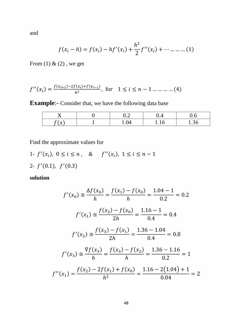
and
( ) ( ) ( )
( ) ( )
From (1) & (2) , we get
( ) ( ) ( ) ( )
( )
Example:- Consider that, we have the following data base
0.6 0.4 0.2 0 X
060. 060. 0619 1 ( )
Find the approximate values for
1- ( ) ( )
2- ( ) ( )
solution
( ) ( )
( ) ( )
( ) ( ) ( )
( ) ( ) ( )
( ) ( )
( ) ( )
( ) ( ) ( ) ( )
( )

49
( ) ( ) ( ) ( )
( )
To compute, ( ) ( ) assume now,
( ) ( ) ( )
( )
( ) ( ) ( )
( )
Exercises
Q1: Consider that, we have the following data base
x 0.2 0.4 0.6 0.8 1
y 1.4 1.8 2.2 2.6 3
a. Find where
b. Use Newton’s formulas to find the approximate values of
( ) ( ) ( ) ( ) .
c. Compute the absolute errors at each point.
Q2:- Consider that, we have the following data base
x 0.25 0.5 0.75 1 1.25
y 1 1.4 1.6 2 2.5
Find the approximate values for ( ) ( ) ( )

50
Chapter 5
Numerical integration
In this chapter, we study some methods; used to find the approximate value for the
definite following integral
∫ ( )
( , - , - )
when it’s difficult to find the exact value by using known methods (integration
methods), such as:
∫
The general idea of the integration methods is to divide the interval , -, into of
subintervals :
, - , - , - , -
It is not needed to be the distances between the points * + are equal.
Next, we consider the polynomial ( ) as an approximate form for f .
( ) ( ) , -
which means the problem becomes
∫ ( )
∫ ( )
From the last form, we note that, the formula of numerical integration depends on
the way of choosing the polynomial .
The general formula of integration methods takes the form:
∫ ( )
∫ ( )
∑ ( ) ( )
where,

51
are called the coefficients * +
* + are called the nodes.
If we used Lagrange polynomial, we could very easy get * + , * +
as
follows:
We divide the interval , -, to the n of subintervals
, - , - , - , -
where the distances between the nodes {xi+ are equal
i.e.
Thus ( ) ( ) ( ) , -
where is the Lagrange polynomial
∫ ( )
∫ ( )
∫ ∑ ( ) ( )
∫ ( )( ( ))
( ) ∏ ( )
where ∫ ( )( ( ))
( ) ∏ ( )
is the truncation error formula
∫ ( )
∑ (∫ ( )
) ( )) ……(1),
which means
(∫ ( )
)
In the last formula,
,(Trapezoidal method)For n=1, method is called
Simpson method).)For n=2, method is called

52
Trapezoidal method
From the general form of integration, with choosing Lagrange polynomial, and
n=1, we get
, ,
∫ ( )
∑(∫ ( )
) ( ) ∫ ( ( ))
( )( )
Set , ∫ ( )
∫( )
( )
( )
( )
∫ ( )
∫( )
( )
( )
( )
Substitute in equation (1), we get
∫ ( )
∑ ( )
( )
( )
which is the Trapezoidal formula.
where the truncation error formula takes the form
( ) ∫ ( ( ))
( )( )
( )
Remark:- We note that, if is polynomial of order less than or equal one, then the
truncation error equal zero, which means:
∫ ( )
∑ ( )
( )
( )

53
Example:- Use the Trapezoidal method to find the approximate value of the following
integral
∫( )
Solution
, , ,
∫ ( )
( ( ) ( ))
∫( )
(( ) (
) )
( )
While, we can find the exact value as follows:
∫( )
(
)
Thus, the absolute error is
In order to get more accurate value to the integration, we use the composite
Trapezoidal methods.
Composite Trapezoidal methods
The idea is, we divide the interval , - into n of subintervals
, - , - , - , -
Since the summation of all the integrals on the subintervals is equal the integral on
the whole interval , -, we can apply the Trapezoidal formula, on each of the
integrals as follows:

54
∫ ( )
∫ ( )
∫ ( )
∫ ( )
,
( ( ) ( ))- ,
( ( ) ( ))- ,
( ( ) ( ))
∑
( )
where
∫ ( )
0
( ( ) ( ))1 ∑ ( )
The last equation is called, the Composite Trapezoidal Formula.
Steps of composite Trapezoidal algorithm
1-Input
2- Input the number of partitions n
3-Define the function ( )
4-Find
5- Use composite Trapezoidal formula
∫ ( )
[
( ( ) ( ))] ∑ ( )
Example: For the last example, find the approximate value of the integral, using
composite Trapezoidal methods with taking
∫ ( )

55
, - , - , -
∫ ( )
∫ ( )
∫ ( )
,( ) (
) -
,( ) ,(
) -
=1/4(1+1/8+1+1/8+1+2)= 1/4[21/4]=[21/16]=1.3125
E=| - |=|1.31-1.25|=0.06
Remark
In last example, it is clear that, from the absolute errors, the result of the composite
Trapezoidal method is more accurate than the result that we get by using normal
Trapezoidal method.
Matlab Code for composite Trapezoidal method
Next, we write dawn the Matlab Code for last example with
a=0; b=1; n=40;
h=(b-a)/n; g=0;
x=sym('x');
f=x^3+1;
m=subs(f,x,a)+subs(f,x,b);
for i=1:n-1
d=a+i*h;
g=g+2*subs(f,x,d);
end
T=(h/2)*(m+g);

56
fprintf('I=%f',T);
I=1.250156
Simpson method
Here, we set , which means
, - , - , -
We use Lagrange polynomial, of order 2, to find an approximate form for the
function f .
( ) ( ) , -
∫ ( )
∑(∫ ( )
) ( ) ∫ ( ( ))
( )( )( )
we can show that:
∫ ( )
∫ ( )
∫ ( )
( ) ∫ ( ( ))
( )( )( )
( )( ) ( )
Thus, we get
∫ ( )
( )
( )
( )
which is the Simpson integral formula

57
Remark:- We note that, if is polynomial of order less than or equal 3, then the
truncation error equal zero, which means:
∫ ( )
∑ ( )
( )
( )
( )
Example: find the approximate value of the following integral , using Simpson
method
∫
Solution:
, - , - , -
∫
,
|
|
-
=
, ( ) -
H.W. Find the following integral, by using Simpson method.
∫ ( )
(1.25, answer)
Composite Simpson method
We divide, the interval , -, into pairs of subintervals, where (n
should be odd ), as follows:
, - (, - , -) ( , - , -) (, - , -)

58
Apply Simpson formula for each of the pairs of subintervals
∫ ( )
∫ ( ) ∫ ( )
∫ ( )
, ( ) ( ) ( )-
, ( ) ( ) ( )-
, ( ) ( )
( )- ∑
( )( )
where
∫ ( )
, ( ) ( )-
∑ ( )
∑ ( )
which is the ‘Composite Simpson Integral formula ‘
Steps of composite Simpson algorithm
1-Input a,b
2-Input the numbers of the pairs of subintervals, , and set
3-Define the function f
4-
5-Use the composite Simpson integral formula,
∫ ( )
, ( ) ( )-
∑ ( )
∑ ( )

59
Example:- Use Composite Simpson integral formula to find the value of the
following integral, consider n=4
∫
solution
[ - (, - , -) (, - , -)
∫
∫ ∫
Apply Simpson formula for each integral, we get that
∫
(
)
(
)
=
( ( ) )
( ( ) ) 15.0375
Remark: If we increase n, ( ), we can get more accurate
results to the integration.
H.W. Compare between the two absolute errors, those can arise from using
Simpson method with n=2 and 4, respectively, to find the approximate value
for the following integral:
∫ ( )

60
Matlab Code for composite Simpson method
Next, we write dawn the Matlab Code for which can be used to find the following
integer ∫ ( )
using composite Simpson method, with .
a=0; b=1; n=40;
h=(b-a)/n; g=0;
x=sym('x');
f=x^3+1;
m=subs(f,x,a)+subs(f,x,b);
r=0; g=0;
for i=1:n-1
d=a+i*h;
if rem(i,2)==0
r=r+2*subs(f,x,d);
else
g=g+4*subs(f,x,d);
end
end
T=(h/3)*(m+r+g);
fprintf('I=%f',T);
I=1.25
Note that
and that because is a polynomial of order three.

61
Exercises
Q1: Use both of Trapezoidal and composite Simpson formulas to derive a
new composite formula, with n=5.
a. What is the truncation error’s form of this new formula?
b. What should be the degree of to guarantee that there is no absolute error.
c. Use the new formula to find the approximate value of the following integral,
and find the absolute error.
∫
Q2: Use Trapezoidal method, with n=1, and n=3 to find the approximate value of
the following integral, and find the absolute error in each case.
∫( )

62
Chapter 6
Numerical Solutions of First Order Ordinary Differential
Equations
It is well known that, an ordinary differential equation (O.D.E.), is an
equation has unknown function y, of one variable x, and some of its
derivatives. For instance
while, partial differential equation, has unknown function of two or more variables
and some of its partial derivatives. For instance
The order of the differential equation, is the highest derivative appears in the
differential equation.
In this chapter, we will study, the numerical solutions for first order ordinary
differential equations, which takes the general form:
( )
The solution of the differential equation above, is an differentiable function
defined on an interval , -, and satisfies the differential equation. Each solution
has a constant c, which can be determined, if y is known for at least one point
, -. ( ( ) initial condition )
Remark : The problem of the differential equation with an initial condition is
called Initial Value Problem:
( ) ( )
Example:
( )

63
While, if y are given at more than one point, then the problem is called
Boundary values problem:
Example
( ) ( )
In this chapter, we will only study the numerical solutions of first order
initial vale problems.
Our aim is find the approximate solution, for this problem at certain points:
* + , -, which means, we only need to find * +
Next, we will study some important methods that can be used to find the numerical
solutions of initial value problems
Euler Algorithm
The general idea of this method, is to divide the interval , -, into n of
subintervals, as follows:
( )
In order to find the approximate solution of the initial value problem at the point
, we consider the definition of ( )
( ) →
( ( ) ( )
)
( ) ( )
( ), we obtain since,
( ) ( )
( )
( ) ( ) ( ( ))
Assume that, is the approximate value of ( )

64
( )
The last equation is called Euler formula.
Remark:-
Euler formula, can only be used only for finding the numerical solutions at the
points ) , while if we would like to find the approximate value of
( ) ) , - then in this case, we can use an
interpolation method.
Steps of Euler algorithm
1-Input
2-Input the points,
3-Define ( )
4- Input, n, ( )
5- Set
6-Compute the approximate values of ( ) using Euler formula:
( )
6- If , -
then use a Newton’s finite difference formula,
to find the approximate value of the initial value problem at this point.
Example: - Consider that, we have the following initial value problem
( )
, -
Use Euler method to find the approximate values of y(0.1),y(0.15), y(0.2) and
compare these values with the exact solution (find the absolute errors)
Solution :-
h=
by using Euler formula

65
( )
( )( ( )( ))
( )
( )( ( )( ))
Thus, we get the following database
We can show that, by using separation of variables, the exact solution of this
problem takes the form:
which leads to ( ) ( )
Thus, the absolute errors can be computed as follows:
( )
( )
From the above database, we can compute the approximate value of ( ) , by
using Backward Newton’s formula studied in Chapter 4. (H.W.)
Modified Euler method
In order to get more accurate results than Euler method, we define the modified
Euler method, which has the following general formula
( ( ) (
))
where
( ) Normal Euler

66
In fact, the first equation depends on the second equation, and this way is called
(Estimation–Correction), because from the first equation, we get estimate value
for ( ), and then in the second equation, we get a correction for this value.
The steps of Modified Euler algorithm are the same as the steps of normal Euler
algorithm and we only have to add one step more after step 5, which is:
6- Correct the estimated value that we get from using normal Euler formula,
by using the modified Euler formula.
Example:- Use Modified Euler method for the last example.
Solution
n=2
Estimation: ( )
( )( )
( ( ) (
)) Correction:
( ( )( ))
Estimation: ( )
( )( ( )( ))
( ( ) (
)) Correction:
( )
( ( )( ) ( )( ))
Thus, we get the following data base
0.2 0.1 0 x
0.5 y

67
Next, we compute the absolute errors:
( )
( )
It is clear that, this database is much different from that we have got from using
normal Euler method. Moreover, it is more accurate.
Matlab Codes of Euler methods
For the last example, write Matlab codes, that can be used to find ( ) ( ),
by using Euler & modified Euler methods
Euler
x0=0; y0=0.5;h=0.1; X(1)=x0+h; X(2)=X(1)+h;
x=sym('x');
y=sym('y');
f=-x*y;
for i=1:2
Y(i)=y0+h*subs(f,{x,y},{x0,y0});
x0=X(i); y0=Y(i);
end
disp(Y)
Answer: 0.5 0.4950
Modified Euler
x0=0; y0=0.5;h=0.1; X(1)=x0+h; X(2)=X(1)+h;
x=sym('x');
y=sym('y');
f=-x*y;

68
for i=1:2
Ye(i)=y0+h*subs(f,{x,y},{x0,y0});
Yc(i)=y0+(h/2)*(subs(f,{x,y},{x0,y0})+subs(f,{x,y},{X(i
),Ye(i)}))
x0=X(i); y0=Yc(i);
end
disp(Yc)
Answer: 0.4975 0.4901
Explicit & Implicit Methods
Normal Euler method, belongs to group of methods called explicit methods, and
that because of , computing depends only on ,while modified Euler
methods belongs to implicit methods, and that because of , computing
depends on both of
Runge-Kutta Methods
Since modified Euler method needs two steps to get the solutions, it is considered
a two-steps method. Moreover, Euler methods need to approximate the derivatives
by using special forms. Thus, we will use Runge-Kutta method , which is a one-
step method and it can be used to avoid determining higher order derivatives.
Runge-Kutta Method of order 2:
Set ( )
( )
Recall modified Euler formula
( ( ) (
))
where
( )

69
( )
Runge-Kutta Method of order 4:
Set ( )
(
)
(
)
( )
( )
which is Ruga-Kutta formula of order4.
Example:- Consider that, we have the following intial value problem:
( )
Use Runga-Kutta method of order 2 and order 4 to compute the approximate
values of ( ) ( )
Solution
( ) ( )
( ) ( )
( ) ( )
( ) ( )
( ) ( )

70
( ) ( )
Next, we compute these values by using Euler method of order4
( ) ( )
(
) (
)
(
) (
)
( ) ( )
( )
( ( ) ( ) )
( ) ( )
(
) (
)
(
) (
)
( ) ( )
( )
( ( ) ( ) )
Since is linear equation, we can show that, by using integration factor,
the exact solution of problem in the last example takes the form:

71
Thus ( ) ( )
Thus, the absolute errors, obtained by Ruge-Kutta of order 2 are as follows:
( )
( )
while, the absolute errors, obtained by Ruge-Kutta of order 4 are as follows:
( )
( )
It is clear that, the results of Ruga-Kutta method of order 4 are much accurate than
the results of Ruga-Kutta method of order 2.
Matlab Codes for Runge-Kutta Methods
We can write matlab codes that can be used to solve the last example by using
Ruga-Kutta method of order 2 and 4, as follows:
Order2
x0=0; y0=1; h=0.25;
X(1)=0.25; X(2)=0.5;
x=sym('x');
y=sym('y');
f=x+y;
for i=1:2
k1=subs(f,{x,y},{x0,y0});
k2=subs(f,{x,y},{x0+h,y0+h*k1});
Y(i)=y0+(h/2)*(k1+k2);
x0=X(i);
y0=Y(i);
end
disp(Y)

72
1.3125 1.7832
Order4
x0=0; y0=1; h=0.25;
X(1)=0.25; X(2)=0.5;
x=sym('x');
y=sym('y');
f=x+y;
for i=1:2
k1=subs(f,{x,y},{x0,y0});
k2=subs(f,{x,y},{x0+h/2,y0+h/2*k1});
k3=subs(f,{x,y},{x0+h/2,y0+h/2*k2});
k4=subs(f,{x,y},{x0+h,y0+h*k3});
Y(i)=y0+(h/6)*(k1+2*k2+2*k3+k4);
x0=X(i);
y0=Y(i);
end
disp(Y)
1.3180 1.7974
Exercises
Q1: Consider the following initial value problem:
( ) .
a. Use Runge-Kutta method of order 2 to find the approximate values of
( ) ( ) ( ) ( )
b. Depending on the results of a. , find the approximate value of ( )
c. Find the absolute error at each point in a.
Q2: Consider the following initial value problem:
( )

73
, -
a. Use Modified Euler method to find the approximate values for * +
b. Find the absolute error at each point.